Revisiting Degeneracy, Strict Feasibility, Stability,
in
Linear Programming

Haesol Im Thanks: Department of Combinatorics and Optimization Faculty of Mathematics, University of Waterloo, Waterloo, Ontario, Canada N2L 3G1; Henry Wolkowicz Thanks: Department of Combinatorics and Optimization Faculty of Mathematics, University of Waterloo, Waterloo, Ontario, Canada N2L 3G1; Research supported by The Natural Sciences and Engineering Research Council of Canada; www.math.uwaterloo.ca/~hwolkowi.

Abstract

Currently, the simplex method and the interior point method are indisputably the most popular algorithms for solving linear programs, LPs. Unlike general conic programs, LPs with a finite optimal value do not require strict feasibility in order to establish strong duality. Hence strict feasibility is seldom a concern, even though strict feasibility is equivalent to stability and a compact dual optimal set. This lack of concern is also true for other types of degeneracy of basic feasible solutions in LP. In this paper we discuss that the specific degeneracy that arises from lack of strict feasibility necessarily causes difficulties in both simplex and interior point methods. In particular, we show that the lack of strict feasibility implies that every basic feasible solution, BFS, is degenerate; thus conversely, the existence of a nondegenerate BFS implies that strict feasibility (regularity) holds. We prove the results using facial reduction and simple linear algebra. In particular, the facially reduced system reveals the implicit non-surjectivity of the linear map of the equality constraint system. As a consequence, we emphasize that facial reduction involves two steps where, the first guarantees strict feasibility, and the second recovers full row rank of the constraint matrix. This illustrates the implicit singularity of problems where strict feasibility fails, and also helps in obtaining new efficient techniques for preproccessing. We include an efficient preprocessing method that can be performed as an extension of phase-I of the two-phase simplex method. We show that this can be used to avoid the loss of precision for many well known problem sets in the literature, e.g., the NETLIB problem set.

Keywords: linear programming, facial reduction, preprocessing, degeneracy, implicit problem singularity

AMS Classification: 90C05, 90C49.

1 Introduction

The Slater condition (strict feasibility) is a useful property for optimization models to have. Unlike general conic programs, linear programs (LPs) do not require strict feasibility as a constraint qualification to guarantee strong duality, and therefore, it is often not discussed. In fact, degeneracy in general is not considered to be a serious concern in linear programming. The Goldman-Tucker Theorem [29] is related in that it guarantees a primal-dual optimal solution satisfying strict complementarity $x^{*}+z^{*}>0$ for the standard form LP. However, it does not guarantee the existence of a strictly feasible primal solution $\hat{x}>0$ . The lack of strict feasibility for an LP does not seem to cause problems at first glance, especially when the simplex method is used. In this manuscript, we show that the failure of strict feasibility results in degeneracy problems when simplex-type methods are used. More specifically, the lack of strict feasibility inevitably renders LPs degenerate, i.e., every basic feasible solution is degenerate.¹¹ 1 Conversely, if we can find one nondegenerate basic feasible solution, then strict feasibility holds. Note that strict feasibility along with full row rank of the linear constraint is the Mangasarian-Fromovitz constraint qualification [37]. This is equivalent to a compact dual optimal set and is equivalent to stability with respect to perturbations of the right-hand side.

The simplex method [16] is one of the most popular and successful algorithms for solving linear programs. Degeneracy, a zero basic variable, could result in cycling and noncovergence. There are many anti-cycling rules, see e.g., [34, 17, 7, 50, 26] and the references therein. However, techniques for the resolution of degeneracy often result in stalling [45, 12, 6, 38], i.e., result in taking a large number of iterations before leaving a degenerate point and can even fail to leave with current techniques [34]. Degeneracies are known to cause numerical issues when interior point methods are used, e.g., [33]. For example, degeneracy can result in singularity of the Jacobian of the optimality conditions, and thus also in ill-posedness and loss of accuracy [31]. We note that the method most often used in the literature when converting a problem that has a free variable into standard form, is to replace the free variable by the difference of two nonnegative variables. This results in an unbounded primal optimal set and strict feasibility failing for the dual problem, i.e., from our work we see that this standard approach changes a well-posed problem into an ill-posed one.

Our main results on the degeneracy arising from loss of strict feasibility are shown using the effective preprocessing tool called facial reduction, FR. For a problem lacking strict feasibility, facial reduction strives to formulate an equivalent problem that has a Slater point. By examining the facially reduced system, we obtain two results. First, we show that every basic feasible solution is degenerate when strict feasibility fails. This leads to an efficient approach for eliminating variables that are fixed at $0$ . Second, we investigate implicit redundancies as a source of instability arising in problems where strict feasibility fails. We see that the linear map of the facially reduced system is non-surjective, i.e., the original constraints are implicitly redundant. Finally, we use these results to develop an efficient preprocessing technique to obtain strict feasibility. This technique is illustrated on instances from the NETLIB data set.

The contribution of this manuscript is threefold; (i) We provide the complete description of the facially reduced system of a linear program and introduce related notions of singularity; (ii) We show that every basic feasible solution of a standard linear program is degenerate when strict feasibility fails; (iii) We propose and illustrate an efficient preprocessing scheme that can be performed as an extension of phase-I of the two-phase simplex method. This technique allows for eliminating variables fixed at $0$ , and thus regularizing and simplifying the LP.

The manuscript is organized as follows. In Section 2 we present the background and notations. Included are the notions of degeneracy, facial reduction and three types of singularity degree. We then describe what facial reduction tries to achieve. In Section 3 we present our main result and immediate corollaries, as well as the efficient preprocessing method that can be used as an extension of phase-I of the two-phase simplex method. In addition, we relate our main result to known results in the literature, such as distance to infeasibility. In Section 4 we illustrate algorithmic performance of interior point methods and the simplex method under the lack of strict feasibility. We present our conclusions in Section 5.

2 Preliminaries

2.1 Background and Notation

We let $\mathbb{R}^{n},\mathbb{R}^{m\times n}$ be the standard real vector spaces of $n$ -coordinates and $m$ -by- $n$ matrices, respectively. We use $\mathbb{R}_{+}^{n}$ ( $\mathbb{R}_{++}^{n}$ , resp.) to denote the $n$ -tuple with nonnegative (positive) entries. We use $\langle\cdot,\cdot\rangle$ to denote the usual inner product. Given a vector $x\in\mathbb{R}^{n}$ , we let $\supp(x)$ to denote the index set $\{i:x_{i}\neq 0\}$ . Given a matrix $A\in\mathbb{R}^{m\times n}$ , we adopt the MATLAB notation to denote a submatrix of $A$ . Given a subset ${\mathcal{I}}$ of column indices, $A_{\mathcal{I}}\in\mathbb{R}^{m\times|{\mathcal{I}}|}$ is the submatrix of $A$ that contains the columns of $A$ in ${\mathcal{I}}$ . We also use the notation $A_{\mathcal{I}}$ to denote $A_{\mathcal{I}}$ when the meaning is clear. Given a convex set ${\mathcal{C}}$ , $\relint({\mathcal{C}})$ denotes the relative interior of the set ${\mathcal{C}}$ .

Throughout this manuscript, we work with feasible LPs in standard form with finite optimal value:

({\mathcal{P}})\qquad{\@index{\@indexphrase{$p^{*}$}}}\ignorespaces\textit{$p^{*}$}=\min_{x}\left\{c^{T}x\ :\ Ax=b,\ x\geq 0\right\},

where $p^{*}\in\mathbb{R},A\in\mathbb{R}^{m\times n},b\in\mathbb{R}^{m}$ and $c\in\mathbb{R}^{n}$ . We assume that $\rank(A)=m$ , i.e., there is no redundant constraint. We use ${\mathcal{F}}$ to denote the feasible region of ( ${\mathcal{P}}$ )

{\mathcal{F}}=\{x\in\mathbb{R}^{n}:Ax=b,\ x\geq 0\}.

(2.1)

2.1.1 Degeneracy in LP

Given an index set ${\mathcal{B}}\subset\{1,\ldots,n\},|{\mathcal{B}}|=m$ , a point $x\in{\mathcal{F}}$ is called a basic feasible solution, BFS , if $A_{\mathcal{B}}$ is nonsingular and $x_{i}=0,\ \forall i\in\{1,\ldots,n\}\setminus{\mathcal{B}}$ . It is well-known that the simplex method iterates from BFS to BFS. A basic feasible solution $x\in{\mathcal{F}}$ is nondegenerate if $x_{i}>0,\ \forall i\in{\mathcal{B}}$ ; it is degenerate if $x_{i}=0$ , for some $i\in{\mathcal{B}}$ . It is clear that every basic feasible solution has at most $m$ positive entries.²² 2 We mainly consider primal degeneracy here, though everything follows through for dual degeneracy. In fact, there are clear connections from complementary slackness between variables positive in every BFS and dual variables fixed at $0$ .

We partition the index set $\{1,\ldots,n\}$ as

\{1,\ldots,n\}={\mathcal{I}}_{+}\cup{\mathcal{I}}_{0},\text{ where }{\@index{\@indexphrase{${\mathcal{I}}_{0}:=\{i\,:\,x_{i}=0,\forall x\in{\mathcal{F}}\}$}}}\ignorespaces\textit{${\mathcal{I}}_{0}:=\{i\,:\,x_{i}=0,\forall x\in{\mathcal{F}}\}$}\text{ and }{\@index{\@indexphrase{${\mathcal{I}}_{+}=\{1,\ldots,n\}\backslash{\mathcal{I}}_{0}$}}}\ignorespaces\textit{${\mathcal{I}}_{+}=\{1,\ldots,n\}\backslash{\mathcal{I}}_{0}$},

i.e., ${\mathcal{I}}_{0}$ denotes the variables fixed at $0$ . Note that fixed variables are identified during preprocessing in the literature if the upper and lower bounds are equal, e.g., [39, 2, 35]. However, the set ${\mathcal{I}}_{0}$ is not as easily identified.

There are in fact several types of degeneracy. Let $\bar{x}$ be a given BFS with basis ${\mathcal{B}}$ . (Wlog ${\mathcal{B}}=\{1,\ldots,m\}$ .) We can write the equivalent canonical form representation of the feasible set using the basis at $\bar{x}$ :

{\mathcal{F}}=\left\{x=\begin{pmatrix}x_{\mathcal{B}}\cr x_{\mathcal{N}}\end{pmatrix}\,:\,x_{\mathcal{B}}=b-A_{\mathcal{B}}^{-1}A_{\mathcal{N}}x_{\mathcal{N}}\geq 0,x_{\mathcal{N}}\geq 0\right\}.

(2.2)

In this form $x_{\mathcal{N}}\in\mathbb{R}_{+}^{n-m}$ , we have $n$ inequality constraints, and we see that degeneracy is equivalent to having an active set with cardinality greater than $n-m$ . This divides into two types corresponding to the sets ${\mathcal{I}}_{0},{\mathcal{I}}_{+}$ , respectively: (i) inequalities that are active in every BFS and correspond to variables in ${\mathcal{I}}_{0}$ above; (ii) those that are not active in at least one BFS. The geometry of (i) is clear as there is no Slater point and ${\mathcal{F}}$ is a subset of a face of the nonnegative orthant. For (ii) the geometry is that some of the constraints are redundant in one of two ways, i.e., that discarding them does not change the feasible set nor the optimality conditions if $\bar{x}$ is optimal.

Remark 2.1.

We note that adding redundant constraints is done in e.g., [19, 18] to show that the central path for interior point methods can follow the boundary closely, i.e., behave very poorly. These redundant constraints correspond to a positive variable in each BFS, i.e., to an inequality in equation 2.2 that is never active. Complementary slackness implies that they correspond to variables fixed at $0$ in the dual problem, thus emphasizing that FR on the dual could avoid some of these difficulties.

2.2 Facial Reduction

In this section we describe the concept of facial reduction and present the properties that are used to establish the main result. We emphasize in this paper that facial reduction for ( ${\mathcal{P}}$ ) involves two steps: first, obtain an equivalent problem with strict feasibility; second, recover full row rank of the constraint matrix. Note that full row rank is always lost during the first step.

Let $K\subset\mathbb{R}^{n}$ be a convex set. A convex set $F\subseteq K$ is called a face of $K$ , denoted $F\unlhd K$ , if for all $y,z\in K$ with $x=\frac{1}{2}(y+z)\in F$ , we have $y,z\in F$ . Given a convex set ${\mathcal{C}}\subseteq K$ , the minimal face for ${\mathcal{C}}$ is the intersection of all faces containing the set ${\mathcal{C}}$ .

Proposition 2.2.

[22, Theorem 3.1.3](theorem of the alternative) For the feasible system of equation 2.1, exactly one of the following statements holds:

1.

There exists $x\in\mathbb{R}^{n}_{++}$ with $Ax=b$ , i.e., strict feasibility holds;
2.

There exists $y\in\mathbb{R}^{m}$ such that

$0\neq z:=A^{T}y\in\mathbb{R}^{n}_{+},\ \text{ and }\ \langle b,y\rangle=0.$ (2.3)

2.2 gives rise to a process called facial reduction. The facial reduction, FR, for an LP is a process of identifying the minimal face of $\mathbb{R}^{n}_{+}$ containing the feasible set ${\mathcal{F}}=\{x\in\mathbb{R}_{+}^{n}:Ax=b\}$ . By finding the minimal face, we can work with a problem that lies in a smaller dimensional space and that statisfies strict feasibility. The FR process, i.e., finding the minimal face, is usually done by solving a sequence of auxiliary systems equation 2.3. More details on FR on general conic problems can be found in [8, 9, 22, 47, 42].

We now describe how the set ${\mathcal{F}}$ (see equation 2.1) is represented after FR. Suppose that strict feasibility fails. Then 2.2 implies that there must exist a nonzero $y\in\mathbb{R}^{m}$ satisfying

\langle x,A^{T}y\rangle=\langle Ax,y\rangle=\langle b,y\rangle=0,\ \forall x\in{\mathcal{F}}.

(2.4)

Hence, every $x\in{\mathcal{F}}$ is perpendicular to the nonnegative vector $z=A^{T}y$ . We call this vector $z=A^{T}y$ an exposing vector for ${\mathcal{F}}$ , and let the cardinality of its support be $s_{z}=|\{i:z_{i}>0\}|$ . Then $z=\sum\limits_{j=1}^{s_{z}}z_{t_{j}}e_{t_{j}}$ , where $t_{j}$ is in increasing order. We now have

0=\langle z,x\rangle\ \text{ and }\ x,z\in\mathbb{R}_{+}^{n}\ \implies\,x_{i}z_{i}=0,\ \forall i,

i.e., the positive elements in $z$ identify the corresponding elements in $x$ that are fixed at $0$ . Then $x=\sum\limits_{j=1}^{n-s_{z}}x_{s_{j}}e_{s_{j}}$ , where $s_{j}$ is in increasing order. We define the matrix with unit vectors for columns

V=\begin{bmatrix}e_{s_{1}}&e_{s_{2}}&\ldots&e_{s_{n-s_{z}}}\end{bmatrix}\in\mathbb{R}^{n\times(n-s_{z})}.

Then we have

{\mathcal{F}}=\{x\in\mathbb{R}^{n}_{+}:Ax=b\}=\{x=Vv\in\mathbb{R}^{n}:AVv=b,v\in\mathbb{R}^{n-s_{z}}_{+}\}.

(2.5)

We call this matrix $V\in\mathbb{R}^{n\times(n-s_{z})}$ a facial range vector. The facial range vector restricts the support of all feasible $x$ . We use the identification equation 2.5 throughout this manuscript. This concludes the first step of FR, i.e., identifying all the variables that are fixed at $0$ .³³ 3 Note that this can be done in one step for linear programs, i.e., the singularity degree for LP is one. We discuss this in Section 2.2.

It is known that every facial reduction step results in at least one constraint being redundant, see e.g., [9], [36, Lemma 2.7], and [47, Section 3.5]. For completeness we now include a short proof tailored to LP, see Lemma 2.3.

Lemma 2.3.

Consider the facially reduced feasible set

{\mathcal{F}}_{r}=\left\{v:AVv=b,v\in\mathbb{R}^{n-s_{z}}_{+}\right\}.

Then at least one linear constraint of the LP is redundant.

Proof.

Let $z=A^{T}y$ be the exposing vector satisfying the auxiliary system equation 2.3. And let $V$ be a facial range vector induced by $z$ . Then

0=V^{T}z=V^{T}A^{T}y=(AV)^{T}y=\sum_{i=1}^{m}y_{i}((AV)^{T})_{i}.

(2.6)

Since $y\in\mathbb{R}^{m}$ is a nonzero vector, the rows of $AV$ are linearly dependent. ∎

We now see the result of the full two-step facial reduction process, i.e., we get a constraint matrix of full row rank:

{\mathcal{F}}=\{x\in\mathbb{R}^{n}_{+}:Ax=b\}=\{x=Vv\in\mathbb{R}^{n}:P_{\bar{m}}AVv=P_{\bar{m}}b,\ v\in\mathbb{R}^{n-s_{z}}_{+}\},

(2.7)

where $P_{\bar{m}}:\mathbb{R}^{m}\to\mathbb{R}^{\bar{m}}$ , $\bar{m}={\rank(AV)}$ , is the simple projection that chooses the linearly independent rows of $AV$ . This concludes the second step of FR, i.e., guaranteeing the full rank. We include a graphical illustration of the two-step FR process; see Figure 2.1.

Refer to caption — Figure 2.1: A graphical illustration of the two-step facial reduction

For a general conic problem, such as semidefinite programs (SDP), the facial reduction iterations do not necessarily end in one iteration; see [47, 48, 14]. And there is a special name for the minimum length of FR iterations.

Definition 2.4 ([49, Sect. 4]).

Given a spectrahehedron ${\mathcal{S}}$ in a closed convex cone ${\mathcal{K}}$ , the singularity degree, $\sd({\mathcal{S}})$ of ${\mathcal{S}}$ is the smallest number of facial reduction iterations for finding $\face({\mathcal{S}},{\mathcal{K}})$ , the minimal face of ${\mathcal{K}}$ containing ${\mathcal{S}}$ .

It is known that FR for LPs can be done in one iteration, i.e., $\sd({\mathcal{F}})\leq 1$ ; see [22, Theorem 4.4.1]. 2.2 and Lemma 2.3 imply that any solution to the system (2.3) gives rise to a strict reduction in the number of variables and the number of equality constraints. This gives rise to the following two novel notions of singularity.

Definition 2.5.

Let $K\subseteq\mathbb{R}^{n}$ be a closed convex cone with corresponding feasible set ${\mathcal{S}}=\{x\in K\,:\,Ax=b\}$ and facially reduced feasible set $\{v\in PK\,:\,(PA{\mathcal{V}})(v)=Pb,v\in\mathbb{R}^{r}\}$ , where $PA{\mathcal{V}}$ is onto $\mathbb{R}^{m_{r}}$ and $PK$ is the cone defined over the smaller dimensional space. Then the implicit problem singularity, $\ips({\mathcal{S}})=m-m_{r}$ .
Moreover, the max-singularity degree of ${\mathcal{S}}$ , denoted $\maxsd({\mathcal{S}})$ , is the largest number of nontrivial facial reduction iterations for finding $\face({\mathcal{S}},K)$ .

The singularity degree is used in [49, Sect. 4] for providing a Hölder regularity constant for semidefinite programs. This is then used in [21] to derive a convergence rate for alternating projection methods for semidefinite programs. Note that $\maxsd({\mathcal{S}})$ can be a larger lower bound of $\ips({\mathcal{S}})$ than $\sd({\mathcal{S}})$ , since at least one linear constraint becomes redundant at each FR iteration. The effect on ill-conditioning of larger values of $\ips$ is seen empirically in Section 4.1.5.⁴⁴ 4 Definition 2.5 can be used to strengthen the upper bound on the rank of SDP solutions in [36], i.e., we get $t(r)\leq m-\ips({\mathcal{S}})\leq m-\maxsd({\mathcal{S}})\leq m-\sd({\mathcal{S}})\leq m$ , where $t(r)$ is the triangular number of the rank $r$ .

2.2.1 Preprocessing in LP

An essential step for simplex and interior point methods is preprocessing, see e.g., [39, 2, 30, 35] and the references therein. One specific preprocessing step refers to detecting a fixed variable. These are generally detected when the upper and lower bounds on a variable are equal. Fixed variables can also be detected when an invertible block $A_{11}$ can be isolated $A=\begin{bmatrix}A_{11}&A_{12}=0\cr A_{21}&A_{22}\end{bmatrix},\,b=\begin{pmatrix}b_{1}\cr b_{2}\end{pmatrix}$ . With $x=\begin{pmatrix}x_{1}\cr x_{2}\end{pmatrix}$ , we can eliminate $x_{1}=A_{11}^{-1}b_{1}$ and discard the first block of now redundant rows, along with the first block of columns. If $b_{1}=0$ then we have trivially identified variables fixed at zero and removed redundant rows and columns. The remaining block $A_{22}$ remains full row rank as happens in Gaussian elimination.

In general, FR for linear programs refers to identifying variables fixed at $0$ , and removing them along with corresponding columns and redundant rows. In general, this is not as simple as above, and the theorem of the alternative is needed. As a consequence of our main result, we see below that a single step of the simplex method, a phase-I part B approach, yields many of these variables that are identically zero on the feasible set.

One of the standard assumptions in linear programming is full row rank of $A$ . As we observed in Lemma 2.3, each FR step results in linear dependence of the constraints. We now summarize two available methods for extracting a maximal linearly independent subset of rows of $AV$ . The first method uses a rank-revealing QR decomposition⁵⁵ 5 https://www.mathworks.com/matlabcentral/fileexchange/77437. Let $M=(AV)^{T}$ . Let $MI(:,\pi)=QR$ be a QR factorization where $\pi$ is a permutation vector, $Q$ is a orthogonal matrix and $R$ is an upper triangular matrix with a non-increasing diagonal in absolute value. The matrix $I(:,\pi)$ permutes the columns of $M$ . If $M$ has linearly dependent columns, then the matrix $R$ contains zeros on its diagonal. Let $r$ be the number of the nonzero diagonal entries of $R$ . Then, $\pi(1:r)$ returns the subset of columns indices of $M$ that are linearly independent. Another available method makes use of artificial variables [15, Box 8.2]. It constructs $\begin{bmatrix}I&AV\end{bmatrix}$ and sets the initial basis matrix to be the first $m$ columns. Then it performs a variant of the phase-I of the two-phase simplex method to drive the basic variables out of the basis one by one. When such an operation is not applicable, a linearly dependent row of $AV$ is detected. Computational improvements of this method are made in [1, 40]. A more recent method is the rank revealing Gaussian elimination by the maximum volume concept given in [46].

3 Main Result and Consequences

In this section we present our main result, see Theorem 3.1. We provide two proofs: one takes an algebraic approach by using the definition of the basic feasible solution; and the other takes a geometric approach by using extreme points. Both proofs rely heavily on Lemma 2.3. In Section 3.2 we present an efficient preprocessing scheme that can be used as an extension of the phase-I of the two-phase simplex method. In Section 3.3 we include immediate corollaries of the main result and interesting discussions.

3.1 Lack of Strict Feasibility and Relations to Degeneracy

Theorem 3.1.

Suppose that strict feasibility fails for ${\mathcal{F}}$ . Then every basic feasible solution to ${\mathcal{F}}$ is degenerate.

3.1.1 An Algebraic Proof of Theorem 3.1 via the Definition of BFS

Proof.

Since there is no strictly feasible point in ${\mathcal{F}}$ , there exists a facial range vector $V$ , and as in equation 2.5 we have

{\mathcal{F}}=\{\ x\ =Vv\in\mathbb{R}^{n}\ :\ AVv=b,\ v\in\mathbb{R}^{n-s_{z}}_{+}\ \}.

By Lemma 2.3, $AV$ has at least one redundant row. By permuting the columns of $A$ , we may assume that the matrix $V$ is of the form

V=\begin{bmatrix}I_{r}\\ 0\end{bmatrix}\text{ and }r=n-s_{z}.

We partition the index set $\{1,\ldots,n\}$ as

\{1,\ldots,n\}={\mathcal{I}}_{+}\cup{\mathcal{I}}_{0},\text{ where }{\mathcal{I}}_{+}=\{1,\ldots,r\}\text{ and }{\mathcal{I}}_{0}=\{r+1,\ldots,n\}.

Then we have $A=\begin{bmatrix}A_{{\mathcal{I}}_{+}}&A_{{\mathcal{I}}_{0}}\end{bmatrix}$ . Let $\bar{x}\in{\mathcal{F}}$ be a basic feasible solution with basic indices

{\mathcal{B}}\subset\{1,\ldots,n\},\ |{\mathcal{B}}|=m,\ \det(A_{\mathcal{B}})\neq 0,\ \text{ and }\ A_{\mathcal{B}}\bar{x}({\mathcal{B}})=b.

Suppose ${\mathcal{B}}\subseteq{\mathcal{I}}_{+}$ . We note, by Lemma 2.3 again, that $A_{{\mathcal{I}}_{+}}=AV$ has linearly dependent rows, i.e., $\rank(A_{{\mathcal{I}}_{+}})<m$ . Hence $\bar{x}$ must include a basic variable in ${\mathcal{I}}_{0}$ and this concludes that every basic feasible solution is degenerate. ∎

3.1.2 A Geometric Proof Using Extreme Points

We now give the second proof of our main result. Suppose that $X\in F$ with $\rank(X)=r$ , where $F$ is a face of the set $\{X\in\mathbb{S}^{n}_{+}:\trace(A_{i}X)=b_{i},\forall i=1,\ldots,m\}$ . Here, $\mathbb{S}^{n}_{+}$ denotes the set of $n$ -by- $n$ positive semidefinite matrices. It is known that $\frac{r(r+1)}{2}\leq m+\dim F$ , see [41, Theorem 2.1]. We rewrite [41, Theorem 2.1] in the language of polyhederon in 3.2. We include the proof for completeness in Section A.1.

Corollary 3.2.

([41, Theorem 2.1]) Suppose that $x\in F$ , where $F$ is a face of the set ${\mathcal{F}}$ . Let $r$ be the number of nonzeros in $x$ and $d=\dim F$ . Then the number of nonzero entries of $x\in F$ is at most $m+d$ .

A point $x$ in a convex set ${\mathcal{C}}$ is called an extreme point if, for all $y,z\in{\mathcal{C}}$ , $x=\frac{1}{2}(y+z)$ implies $x=y=z$ . An extreme point is itself a face and the dimension of this face is $0$ . Hence, we obtain 3.3 by writing 3.2 through the lens of extreme points.

Corollary 3.3.

Every extreme point $x\in{\mathcal{F}}$ has at most $m$ positive entries.

We now restate the main result of this paper Theorem 3.1 in the language of extreme points and number of rows of $A$ .

Theorem 3.4.

Suppose that strict feasibility of ${\mathcal{F}}$ fails. Then every extreme point $x\in{\mathcal{F}}$ has at most $m-1$ positive entries.

Proof.

Since strict feasibility fails for ${\mathcal{F}}$ , we have ${\mathcal{F}}=\{x=Vv\in\mathbb{R}^{n}:AVv=b,\ v\in\mathbb{R}_{+}^{n-s_{z}}\}$ ; see equation 2.5. From Lemma 2.3, we note that at least one equality in $AVv=b$ is redundant. Let $P_{\bar{m}}AVv=P_{\bar{m}}b$ be the system obtained after removing redundant rows of $AV$ ; see equation 2.7. Then, by 3.3, every extreme point of the set $\{v\in\mathbb{R}^{n-s_{z}}_{+}:P_{\bar{m}}AVv=P_{\bar{m}}b\}$ has at most $m-1$ nonzero entries. Hence, the statement follows. ∎

3.1.3 Immediate Consequences of Main Result

We first note that Theorem 3.1 and 3.4 are equivalent owing to the well-known characterization:

x\in{\mathcal{F}}\text{ is a basic feasible solution }\iff x\in{\mathcal{F}}\text{ is an extreme point. }

We now highlight that Theorems 3.1 and 3.4 do not merely imply the existence of a single degenerate basic feasible solution; but rather that every basic feasible solution is degenerate. Developing a pivot rule that prevents the simplex method from visiting degenerate points is not possible as it can never avoid degeneracies when strict feasibility fails, as we now illustrate in the following.

Example 3.5.

Consider ${\mathcal{F}}$ with the data

A=\begin{bmatrix}1&1&3&5&2\\ 0&1&2&-2&2\end{bmatrix}\text{ and }b=\begin{pmatrix}1\\ 1\end{pmatrix}.

Consider the vector $y=\begin{pmatrix}1\\ -1\end{pmatrix}$ . Then

A^{T}y=\begin{pmatrix}1&0&1&7&0\end{pmatrix}^{T}\text{ and }b^{T}y=0.

Hence, 2.2 certifies that ${\mathcal{F}}$ does not contain a strictly feasible point. There are exactly six feasible bases in ${\mathcal{F}}$ . The BFS associated with ${\mathcal{B}}\in\{\{1,2\},\{2,3\},\{2,4\}\}$ is $x=\begin{pmatrix}0&1&0&0&0\end{pmatrix}^{T}$ ; and the BFS associated with ${\mathcal{B}}\in\left\{\{1,5\},\{3,5\},\{4,5\}\right\}$ is $x=\begin{pmatrix}0&0&0&0&\frac{1}{2}\end{pmatrix}^{T}$ . Clearly, all BFSs are degenerate.

Recall that strict feasibility is equivalent to the Mangasarian-Fromovitz constraint qualification, [43]. The latter is equivalent to stability with respect to perturbations of $b$ , and to a compact dual optimal set. Therefore, the following 3.6, obtained by writing the contrapositive of Theorem 3.1, is extremely interesting and important. We provide Example 3.7 below to illustrate 3.6.

Corollary 3.6.

Suppose that there exists a nondegenerate basic feasible solution. Then there exists a strictly feasible point $\hat{x}\in{\mathcal{F}}$ .

Example 3.7.

Consider ${\mathcal{F}}$ with the data

A=\begin{bmatrix}1&0&-2&3&-4\\ 0&-1&-2&3&1\end{bmatrix}\text{ and }b=\begin{pmatrix}1\\ 1\end{pmatrix}.

The system ${\mathcal{F}}$ has exactly four feasible bases; the BFS associated with ${\mathcal{B}}\in\{\{1,4\},\{2,4\},\{4,5\}\}$ is $x=\begin{pmatrix}0&0&0&1/3&0\end{pmatrix}^{T}$ and the BFS associated with ${\mathcal{B}}=\{1,5\}$ is $x=\begin{pmatrix}5&0&0&0&1\end{pmatrix}^{T}$ . We note that the BFS associated with ${\mathcal{B}}=\{1,5\}$ is nondegenerate. As 3.6 states, the system ${\mathcal{F}}$ has a strictly feasible point, and it is verified by the point $\frac{1}{10}\begin{pmatrix}4&1&1&4&1\end{pmatrix}^{T}$ .

3.6 provides a useful check for strict feasibility when the simplex method is used, i.e., if there is any simplex iteration that yields a nondegenerate BFS, then it is useful to record that occurrence. We emphasize that recording the occurrence of a nondegenerate iteration is inexpensive and the occurrence gives a certificate of the stability of the LP instance. We revisit 3.6 in Section 3.2.1 below and present an efficient algorithm for obtaining a Slater point from a nongenerate BFS. But, Example 3.8 below shows that the converse of Theorems 3.1 and 3.4 is not true. In other words, strict feasibility holds and every BFS is degenerate.

Example 3.8.

1.

Consider ${\mathcal{F}}$ with the data

$A=\begin{bmatrix}1&0&2&0&-2\\ 1&-3&2&1&-2\end{bmatrix}\text{ and }b=\begin{pmatrix}1\\ 1\end{pmatrix}.$

${\mathcal{F}}$ has exactly four feasible bases and all of them are degenerate; the BFS associated with ${\mathcal{B}}\in\{\{1,2\},\{1,4\}\}$ is $x=\begin{pmatrix}1&0&0&0&0\end{pmatrix}^{T}$ and the BFS associated with ${\mathcal{B}}\in\{\{2,3\},\{3,4\}\}$ is $x=\begin{pmatrix}0&0&1/2&0&0\end{pmatrix}^{T}$ . However, ${\mathcal{F}}$ contains a strictly feasible point $\frac{1}{10}\begin{pmatrix}1&1&5.5&3&1\end{pmatrix}^{T}$ .
2.

Note that the linear assignment problem (marriage problem) has a strictly feasible point but all the BFS are highly degenerate⁶⁶ 6 Note that this is true for the transportation and the assignment problems. Both are highly degenerate at each BFS but satisfy strict feasibility. For example, for the assignment problem order $n$ , the feasible set can be considered to be the doubly stochastic matrices $X$ . The extreme points are the permutation matrices by the Birkoff-Von Neumann theorem. Therefore, each extreme point has exactly $n$ positive elements while there are $m=2n-1$ linearly independent constraints.. Therefore, ${\mathcal{I}}_{0}=\emptyset$ ; the set of variables fixed at $0$ is empty. Moreover, as an LP, the problem is stable with respect to perturbations in the data.

From Examples 3.5 and 3.8, we observe that there are two different types of degeneracies. One involves variables that are $0$ in one BFS but positive in another; the second involves variables fixed at $0$ , i.e., that result in strict feasibility failing. Note that strict feasibility (along with $A$ full row rank) is the Mangasarian-Fromovitz constraint qualification which is equivalent to stability with respect to right-hand side perturbations [28], which is in turn equivalent to a bounded dual optimal set.

Given a BFS $\bar{x}\in{\mathcal{F}}$ , we let the degree of degeneracy of $\bar{x}$ denote the number of $0$ ’s among its basic variables. By exploiting the facially reduced model we can check how degenerate the BFSs of ${\mathcal{F}}$ are.

Corollary 3.9.

Suppose that strict feasibility fails for ${\mathcal{F}}$ , and let ${\mathcal{F}}$ have the facial range vector representation in equation 2.5. Recall that the set of indices ${\mathcal{I}}_{0}=\{i\in\{1,\ldots,n\}:x_{i}=0,\ \forall x\in{\mathcal{F}}\}$ . Let $\bar{x}\in{\mathcal{F}}$ be a basic feasible solution with basis ${\mathcal{B}}$ . Then, the following holds.

1.

The basis ${\mathcal{B}}$ has an nonempty intersection with ${\mathcal{I}}_{0}$ , i.e., ${\mathcal{B}}\cap{\mathcal{I}}_{0}\neq\emptyset$ .
2.

If the degree of degeneracy of $\bar{x}$ is exactly one, with $\bar{x}_{k}=0,k\in{\mathcal{B}}$ , then $x_{k},A_{:,k}$ can be discarded from the problem.
3.

The degree of degeneracy of $\bar{x}$ is at least $m-\rank(AV)$ .
4.

At least $m-\rank(AV)$ number of basic indices of $\bar{x}$ are contained in ${\mathcal{I}}_{0}$ .

Proof.

1.

Let $\bar{x}\in{\mathcal{F}}$ be a basic feasible solution and let ${\mathcal{B}}$ be a basis for $\bar{x}$ . Item 1 follows from the proof and the definition of the set ${\mathcal{I}}_{0}$ of elements $x_{i}$ that are identically zero on the feasible set.
2.

The proof follows from the algebraic proof of Theorem 3.1 given in Section 3.1.1. Since every BFS is degenerate and the basis has a nonempty intersection with ${\mathcal{I}}_{0}$ , the index $k$ must be in ${\mathcal{I}}_{0}$ .
3.

For Item 3, we note that $A_{\mathcal{B}}$ contains linearly independent columns. Then $A_{\mathcal{B}}$ can contain at most $\rank(AV)$ number of columns from $AV$ . Thus, $\bar{x}({\mathcal{B}})$ must contain at least $m-\rank(AV)$ number of zeros.
4.

Item 4 is a direct consequence of Item 1 and Item 3.

∎

Items 3 and 4 of 3.9 are closely related to the implicit problem singularity, $\ips$ , and the max-singularity degree, $\maxsd$ ; see Definition 2.5. In particular, $\ips({\mathcal{F}})$ is a lower bound of the degree of degeneracy of every BFS of ${\mathcal{F}}$ ; the more implicit redundancies ${\mathcal{F}}$ contains, the more degenerate every BFS becomes. We include an alternative way to view 3.9 in Section 3.1.2.

We conclude the discussions with the following interesting observation. This again illustrates the implicit singularity of the constraints when the Slater condition fails.

Corollary 3.10.

Suppose that strict feasibility fails for ${\mathcal{F}}$ and that $m=1$ . Then the trivial $x^{*}=0$ is an optimal solution.

3.2 Efficient Preprocessing for Facial Reduction and Strict Feasibility

In this section we present an efficient preprocessing method for obtaining a facially reduced system. In Section 3.2.1 we discuss obtaining a strictly feasible point using a nondegeneate BFS and its variant. In Section 3.2.2 we consider the general case of finding an exposing vector to obtain the facially reduced strictly feasible LP.

3.2.1 Towards a Strictly Feasible Point from a Nondegenerate BFS

By 3.6, the existence⁷⁷ 7 Determining the existence of a degenerate basic feasible solution is an NP-complete problem; see [11]. of a nondegenerate BFS guarantees the existence of a strictly feasible point. We now propose a process for acquiring a Slater point from a nondegenerate BFS, and include a generalization. The arguments in this section also provide a constructive proof of 3.6.

Let $\bar{x}\in{\mathcal{F}}$ be a nondegenerate BFS. Without loss of generality, we assume that the (all positive) basic variables $\bar{x}_{\mathcal{B}}$ of $\bar{x}$ are located at the last $m$ entries of $\bar{x}$ . We fix a scalar $\hat{\gamma}\in(0,1)$ and an index $j\in\{1,\ldots,n-m\}$ . For some $\alpha\geq 0$ , we consider the simplex method ratio test type inequality

\hat{\gamma}\bar{x}_{\mathcal{B}}-\alpha(A_{\mathcal{B}})^{-1}A_{j}\geq 0.

(3.1)

Since $\bar{x}_{\mathcal{B}}>0,\hat{\gamma}>0$ , there exists a positive $\alpha$ that maintains the inequality equation 3.1. Let

\alpha^{*}=\min\left\{1,\ \max\{\alpha\in\mathbb{R}_{+}:\hat{\gamma}\bar{x}_{\mathcal{B}}-\alpha(A_{\mathcal{B}})^{-1}A_{j}\geq 0\}\right\},

(3.2)

and decompose

\hat{\gamma}\bar{x}_{\mathcal{B}}=\left(\hat{\gamma}\bar{x}_{\mathcal{B}}-\alpha^{*}(A_{\mathcal{B}})^{-1}A_{j}\right)+\alpha^{*}(A_{\mathcal{B}})^{-1}A_{j}.

We observe that

\begin{array}[]{rcl}b&=&A_{{\mathcal{B}}}\bar{x}_{\mathcal{B}}\\ &=&(1-\hat{\gamma})A_{{\mathcal{B}}}\bar{x}_{\mathcal{B}}+\hat{\gamma}A_{{\mathcal{B}}}\bar{x}_{\mathcal{B}}\\ &=&(1-\hat{\gamma})A_{{\mathcal{B}}}\bar{x}_{\mathcal{B}}+A_{\mathcal{B}}\left(\hat{\gamma}\bar{x}_{\mathcal{B}}-\alpha^{*}(A_{\mathcal{B}})^{-1}A_{j}+\alpha^{*}(A_{\mathcal{B}})^{-1}A_{j}\right)\\ &=&A_{\mathcal{B}}(\bar{x}_{\mathcal{B}}-\alpha^{*}(A_{\mathcal{B}})^{-1}A_{j})+\alpha^{*}A_{j}.\end{array}

If we set $x_{j}=\alpha^{*}>0$ and replace $\bar{x}_{\mathcal{B}}$ by $\bar{x}_{\mathcal{B}}-\alpha^{*}(A_{\mathcal{B}})^{-1}A_{j}$ , then we have increased the cardinality of the positive entries of a solution. We note that $\bar{x}_{\mathcal{B}}-\alpha^{*}(A_{\mathcal{B}})^{-1}A_{j}$ only has strictly positive entries since it it a sum of a positive vector and a nonnegative vector;

\bar{x}_{\mathcal{B}}-\alpha^{*}(A_{\mathcal{B}})^{-1}A_{j}=\underbrace{(1-\hat{\gamma})\bar{x}_{\mathcal{B}}}_{\text{positive}}+\underbrace{\hat{\gamma}\bar{x}_{\mathcal{B}}-\alpha^{*}(A_{\mathcal{B}})^{-1}A_{j}}_{\text{nonnegative}}.

We can continue to increase the number of positive entries of a solution one by one for each $j\in\{1,\ldots,n-m\}$ . Moreover, we can achieve this by a compact vectorized operation. The main idea is that we can choose $\hat{\gamma}$ in equation 3.1 independently for each $j\in\{1,\ldots,n-m\}$ . Let $\gamma_{j}$ be a positive real number such that $0<\gamma:=\sum_{j=1}^{n-m}\gamma_{j}<1$ . Then, we have

\bar{x}_{\mathcal{B}}=(1-\gamma)\bar{x}_{\mathcal{B}}+\gamma\bar{x}_{\mathcal{B}}=(1-\gamma)\bar{x}_{{\mathcal{B}}}+\sum_{j=1}^{n-m}\gamma_{j}\bar{x}_{\mathcal{B}}.

We set an auxiliary matrix

\Theta=\begin{bmatrix}\gamma_{1}\bar{x}_{\mathcal{B}}&\cdots&\gamma_{n-m}\bar{x}_{\mathcal{B}}\end{bmatrix}-(A_{\mathcal{B}})^{-1}A_{1:n-m}\in\mathbb{R}^{m\times(n-m)}

and perform equation 3.2 on each column $j$ of $\Theta$ to obtain the vector $\theta^{*}$ :

\theta^{*}_{j}:=\begin{cases}\max(\Theta(:,j))&\text{ if }\max(\Theta(:,j))\leq 1,\\ 1&\text{ otherwise}.\end{cases}

Then the point

\begin{bmatrix}\theta^{*}\\ \bar{x}_{\mathcal{B}}-(A_{\mathcal{B}})^{-1}A_{1:n-m}\theta^{*}\end{bmatrix}

is a strictly feasible point to ${\mathcal{F}}$ . Hence, this operation provides a constructive proof of 3.6.

We now extend the aforementioned procedure for obtaining a strictly feasible point using any feasible solution $\bar{x}\in{\mathcal{F}}$ such that $A_{\supp(\bar{x})}$ is full row rank. We partition $\bar{x}\in{\mathcal{F}}$ as follows

\bar{x}=\begin{pmatrix}\bar{x}_{{\mathcal{B}}_{1}}\\ \bar{x}_{{\mathcal{B}}_{2}}\\ \bar{x}_{\mathcal{N}}\end{pmatrix},\,\text{ where }\supp(\bar{x})={\mathcal{B}}_{1}\cup{\mathcal{B}}_{2},\ \rank(A_{{\mathcal{B}}_{1})}=m,\ \text{ and }{\mathcal{N}}=\{1,\ldots,n\}\setminus\supp(\bar{x}).

(3.3)

We partition $A$ using the same partition ${\mathcal{B}}_{1}\cup{\mathcal{B}}_{2}\cup{\mathcal{N}}$ :

\begin{bmatrix}A_{{\mathcal{B}}_{1}}&A_{{\mathcal{B}}_{2}}&A_{\mathcal{N}}\end{bmatrix}\bar{x}=b\iff\begin{bmatrix}A_{{\mathcal{B}}_{1}}&A_{\mathcal{N}}\end{bmatrix}\begin{pmatrix}\bar{x}_{{\mathcal{B}}_{1}}\\ \bar{x}_{\mathcal{N}}\end{pmatrix}=\bar{b}:=b-A_{{\mathcal{B}}_{2}}x_{{\mathcal{B}}_{2}}.

Then we can apply the aforementioned procedure to the system

\begin{bmatrix}A_{{\mathcal{B}}_{1}}&A_{\mathcal{N}}\end{bmatrix}\begin{pmatrix}\bar{x}_{{\mathcal{B}}_{1}}\\ \bar{x}_{\mathcal{N}}\end{pmatrix}=\bar{b}

and distribute positive weights to $\bar{x}_{\mathcal{N}}$ using $\bar{x}_{{\mathcal{B}}_{1}}$ . Finally, we find a strictly feasible point to ${\mathcal{F}}$ . This process is summarized in Algorithm 3.1. Furthermore, Algorithm 3.1 provides a constructive proof for 3.11 below.

Proposition 3.11.

Let $x\in{\mathcal{F}}$ be a solution such that $\rank\left(A_{\supp(x)})\right)=m$ . Then, ${\mathcal{F}}$ has a strictly feasible point.

0: Given:

A,\ \bar{x}\in{\mathcal{F}}

partitioned as in equation 3.3.

1: Choose any

\gamma\in\mathbb{R}^{|{\mathcal{N}}|}_{++}

such that

\sum_{j=1}^{|{\mathcal{N}}|}\gamma_{j}<1

2: Compute

\Theta=\begin{bmatrix}\bar{x}_{{\mathcal{B}}_{1}}&\cdots&\bar{x}_{{\mathcal{B}}_{1}}\end{bmatrix}\Diag(\gamma)-A_{{\mathcal{B}}_{1}}^{-1}A_{\mathcal{N}}.

3: Compute

\theta^{*}\in\mathbb{R}_{++}^{|{\mathcal{N}}|}

, where for each

j\in\{1,\ldots,|{\mathcal{N}}|\}

\theta^{*}_{j}:=\begin{cases}\max(\Theta(:,j))&\text{ if }\max(\Theta(:,j))\leq 1,\\ 1&\text{ otherwise}.\end{cases}

4: Set

x^{\circ}=\begin{pmatrix}\bar{x}_{{\mathcal{B}}_{1}}-(A_{{\mathcal{B}}_{1}})^{-1}A_{\mathcal{N}}\theta^{*}\\ \bar{x}_{{\mathcal{B}}_{2}}\\ \theta^{*}\end{pmatrix}

Algorithm 3.1 Compute a Slater Point

3.2.2 Exposing Vector; Phase I Part B; Strict Feasibility Testing

We now present an efficient preprocessing procedure for detecting identically $0$ variables and obtaining exposing vectors in order to get the facially reduced LP. We do this for a given BFS $\bar{x}$ by solving special subproblems using the simplex method. By the end of the process, we determine one of:

1.

a certificate $y$ that produces an exposing vector $A^{T}y$ (Slater condition fails);
2.

a strictly feasible point (Slater condition holds).

This process in fact has two applications. First, since the only requirement of this process is the BFS, the procedure can be considered as an extension of phase-I of the two-phase simplex method that obtains the equivalent facially reduced problem. Second, the procedure can be used as a postprocessing step. We could perform FR on the optimal face and find, and delete, variables fixed at zero in order to improve stability of the optimal solution.

We now describe the proposed preprocessing method. Let ${\mathcal{B}}$ be a degenerate initial basis of ${\mathcal{F}}$ with associated BFS $\bar{x}$ . Without loss of generality, we assume that basic variables are located at the first $m$ entries of $\bar{x}$ . Let $d$ be the degree of degeneracy of $\bar{x}$ . We further assume that the degenerate basic variables are located at the first $d$ entries of $\bar{x}$ . We let ${\mathcal{B}}_{0}:=\{1,\ldots,d\}$ . We now test and record whether or not each $i\in{\mathcal{B}}_{0}$ is a variable fixed at $0$ . Let $i\in{\mathcal{B}}_{0}$ , and consider the following problem:

p^{*}_{i}=\max\{x_{i}\,:\,Ax=b,\,x\geq 0\}.

(3.4)

We may assume that $i=1$ . We solve equation 3.4 using the simplex method from the initial BFS $\bar{x}$ . That is, we do not need to perform the typical phase-I of the two-phase simplex method in order to find a feasible BFS. The optimal value $p_{1}^{*}$ of equation 3.4 is clearly lower bounded by $0$ . We consider two cases below:

1.

Suppose that $x_{1}>0$ after $k$ iterations. Then, the variable $x_{1}$ is not an identically $0$ variable, i.e., we record that $1\in{\mathcal{I}}_{+}$ .
2.

Suppose that $p_{1}^{*}=0$ . Then, the variable $x_{1}$ is an identically $0$ variable, i.e., we record that $1\in{\mathcal{I}}_{0}$ . Let ${\mathcal{B}}^{*}$ be an optimal basis for equation 3.4. Then we have

$y^{*}=A_{{\mathcal{B}}^{*}}^{-T}e_{1},\ \langle b,y^{*}\rangle=0\ \text{ and }A^{T}y^{*}\geq e_{1},$ (3.5)

where $e_{1}$ is the first unit vector of appropriate dimension. We note that the dual optimal solution $y^{*}$ in equation 3.5 produces a solution to the auxiliary system equation 2.3. Therefore, we obtain a nontrivial exposing vector since $0\neq A^{T}y^{*}\geq 0$ .

Let $\{y^{j}\}$ be a collection of the certificates that are obtained from solving equation 3.4 with the index $1$ replaced by $i\in{\mathcal{B}}_{0}$ . Then $y^{\circ}=\sum_{j}y^{j}$ is also a certificate, i.e.,

A^{T}y^{\circ}=\sum_{j}A^{T}y^{j}\geq 0,\ A^{T}y^{\circ}\neq 0,\ \text{ and }\ \langle b,y^{\circ}\rangle=\sum_{j}\langle b,y^{j}\rangle=0,

and we obtain a nontrivial exposing vector $A^{T}y^{\circ}$ for the system ${\mathcal{F}}$ . By summarizing the two cases above, we obtain an efficient preprocessing method Algorithm 3.2.

0: A BFS

\bar{x}

with corresponding basis

{\mathcal{B}}

; set

{\mathcal{B}}_{0}=\{i\in{\mathcal{B}}:\bar{x}_{i}=0\}

1: Initialize:

x^{\circ}=\bar{x}

y^{\circ}=0\in\mathbb{R}^{m}

{\mathcal{J}}_{0}=\emptyset

{\mathcal{B}}_{*}\leftarrow{\mathcal{B}}_{0}

2: while

{\mathcal{B}}_{0}\neq\emptyset

and

{\mathcal{B}}_{*}\neq\emptyset

3: Pick

i\in{\mathcal{B}}_{0}

; starting from the initial BFS

\bar{x}

, solve for primal-dual optima

x^{*},y^{*}

x^{*}=\argmax_{x}\{x_{i}:Ax=b,x\geq 0\},\ \ p^{*}=x_{i}^{*}=b^{T}y^{*}

But, if during the solve,

x_{i}>0

, then stop the iterations; set

x^{*}

as the current point.

{\mathcal{S}}\leftarrow\supp(x^{*})

{\mathcal{B}}_{*}\leftarrow

degenerate basic indices for

x^{*}

6: if

{\mathcal{B}}_{0}\neq\emptyset

and

{\mathcal{B}}_{*}\neq\emptyset

then

7: if

p^{*}=0

(strict feasibility fails) then

8: Use dual certificate

y^{*}

to satisfy equation 2.3

y^{\circ}\leftarrow y^{\circ}+y^{*}

10:

{\mathcal{J}}_{0}\leftarrow{\mathcal{J}}_{0}\cup(\supp(A^{T}y^{*})\cap{\mathcal{B}})

11:

{\mathcal{B}}_{0}\leftarrow{\mathcal{B}}_{0}\setminus\{{\mathcal{S}}\cup{\mathcal{J}}_{0}\}

12: else

13:

{\mathcal{B}}_{0}\leftarrow{\mathcal{B}}_{0}\setminus{\mathcal{S}}

14: end if

15: Choose

\gamma\in(0,1)

and set

x^{\circ}\leftarrow\gamma x^{\circ}+(1-\gamma)x^{*}

16: end if

17: end while

18: if

{\mathcal{J}}_{0}\neq\emptyset

then

19:

z^{\circ}=A^{T}y^{\circ}

(exposing vector)

20:

{\mathcal{R}}\leftarrow

redundant row indices of

A\left(:,\supp(z^{\circ})^{c}\right)

21:

A\leftarrow A({\mathcal{R}}^{c},\supp(z^{\circ})^{c}),\ b\leftarrow b({\mathcal{R}}^{c})

22: else

23: Run Algorithm 3.1 with

x^{\circ}

and

\det(A_{\mathcal{B}})\neq 0

(use

x^{*}

and

{\mathcal{B}}_{*}

, if

{\mathcal{B}}_{*}=\emptyset)

24: end if

Algorithm 3.2 Preprocessing Phase I Part B; Towards Strict Feasibility

The following allows for simplifications in Algorithm 3.2.

Lemma 3.12.

Let ${\mathcal{B}}$ be an initial basis containing the index $i$ for problem (3.4). Then the index $i$ always remains in the basis throughout the iterations.

Proof.

Without loss of generality, we let $i=1$ . We argue that $1$ is not chosen to leave the basis. Let $y^{*}=(A_{\mathcal{B}}^{T})^{-1}c_{\mathcal{B}}$ and $\bar{A}=A_{{\mathcal{B}}}^{-1}A$ . Suppose that the reduced cost at the index $j$ is positive. Then

\begin{array}[]{rcl}0<\bar{c}_{j}=c_{j}-A_{j}^{T}y^{*}=-A_{j}^{T}y^{*}=-A_{j}^{T}(A_{\mathcal{B}}^{T})^{-1}e_{1}=-\bar{A}_{1j}.\end{array}

Since $\bar{A}_{1j}<0$ , the index $1$ is not chosen to leave the basis ${\mathcal{B}}$ . ∎

The following special case is of interest. Namely, no simplex pivoting steps are required to determine strict feasibility.

Theorem 3.13.

(preprocessing for degree of degeneracy $1$ ) Given a basis ${\mathcal{B}}$ , let $\bar{x}$ be a BFS with the degree of degeneracy exactly one and with $\bar{x}_{i}=0,i\in{\mathcal{B}}$ . Let ${\mathcal{N}}=\{1,\ldots,n\}\setminus{\mathcal{B}}$ and let $\bar{y}=(A_{\mathcal{B}}^{T})^{-1}c_{\mathcal{B}},c_{\mathcal{B}}=e_{i}$ . Then strict feasibility fails if, and only if, $\bar{y}$ satisfies $A^{T}_{\mathcal{N}}\bar{y}\geq 0$ .

Proof.

Suppose that $\bar{x}$ is a degenerate BFS with basis ${\mathcal{B}}$ . Without loss of generality, we assume $1\in{\mathcal{B}}$ and $1$ is the degenerate index. We consider the problem

p^{*}_{1}=\max\{x_{1}\,:\,Ax=b,\,x\geq 0\}.

We note that $\langle b,\bar{y}\rangle=0$ since $\langle b,\bar{y}\rangle$ is identical to the current objective value ‘ $0$ ’. The backward direction is clear by 2.2. Now suppose that strict feasibility fails. Suppose to the contrary that $A^{T}_{\mathcal{N}}\bar{y}\geq 0$ fails. Then there exists $j$ such that $A^{T}_{j}\bar{y}<0,\ j\in{\mathcal{N}}$ . Note that, by Lemma 3.12, that $1$ is not chosen to leave the basis. Thus, there is an index $k\neq 1,k\in{\mathcal{B}}$ that leaves the basis. Since all other basic variables are positive, we obtain a positive step length and we improve the objective value, which yields a contradiction to $p^{*}_{1}=0$ . ∎

Upon the termination of Algorithm 3.2, we can always determine whether the system ${\mathcal{F}}$ has a strictly feasible point or not. Algorithm 3.2 terminates in a finite number of iterations since we remove at least one element from the set ${\mathcal{B}}_{0}$ in each iteration. We emphasize that we do not need to solve the auxiliary LPs for all $i\in\{1,\ldots,n\}$ . We solve equation 3.4 only for the degenerate basic indices of the predetermined basis ${\mathcal{B}}$ . However, upon termination of Algorithm 3.2, it is possible that we have not obtained $\face({\mathcal{F}},\mathbb{R}_{+}^{n})$ , the minimal face containing ${\mathcal{F}}$ . Although the complete FR for LP can be completed in one iteration, one step termination is possible only when we find a solution $y$ of equation 2.3 so that $A^{T}y$ is in the relative interior of the conjugate face of $\face({\mathcal{F}},\mathbb{R}_{+}^{n})$ . In this case, we can rerun Algorithm 3.2 with the current facially reduced system. For finding an initial basis for the second trial, we may use the efficient basis recovery scheme [52, Chapter 7].

One of the nice features of Algorithm 3.2 is that we do not need to search for a new initial basis ${\mathcal{B}}$ for each iteration; the initial basis remains the same. Therefore, our approach can be directly employed after the standard phase-I of the two phase simplex method.

We do not need a lot of pivoting steps to determine if $p_{i}^{*}$ is zero or positive. If $p_{i}^{*}=0$ , the initial ${\mathcal{B}}$ is indeed a basis that gives the optimal value. However the dual feasibility may not be obtained immediately⁸⁸ 8 If we have a nondegenerate initial basis, then the dual feasibility is immediately obtained. However, our initial basis is degenerate.. Thus, there may be additional pivots required to obtain the dual feasibility. However, since the optimal value is obtained at ${\mathcal{B}}$ , we do not expect that the optimal basis search to be time-consuming. For the case $p_{i}^{*}\in(0,\infty)$ , the optimal value $p_{i}^{*}$ does not need to be found. Hence once a basis that gives a positive support on $i$ is found, we can terminate the maximization problem in Algorithm 3.2 immediately. We recall from Lemma 3.12 that the index $i$ in equation 3.4 never leaves the basis. In the case of $p_{i}^{*}=\infty$ , we can perform the following operation. Let ${\mathcal{B}}_{c}$ be a basis that indicates $p_{i}^{*}=\infty$ and let $j$ be an entering variable that indicates the unboundedness. Then by setting

x^{\circ}(j)\leftarrow 1,\ x^{\circ}({\mathcal{B}}_{c})\leftarrow x_{{\mathcal{B}}_{c}}-A_{{{\mathcal{B}}_{c}}}^{-1}A_{j}\text{ and }x^{\circ}((\{j\}\cup{\mathcal{B}}_{c})^{c})=0,

we obtain a feasible solution $x^{\circ}$ that yields a positive objective value.

We often get an exposing vector that reveals more than one element in the set ${\mathcal{I}}_{0}$ by solving equation 3.4. Let $p_{1}^{*}=0$ in equation 3.4 and let $y^{*}$ be a dual feasible solution. Suppose that $A^{T}y^{*}=e_{1}$ , i.e., only one exposed variable is revealed. Then $y^{*}\in\nul(A(:,2:n)^{T})$ . Since the data matrix $A$ has more columns than rows, $y^{*}\in\nul(A(:,2:n)^{T})$ generally implies $y^{*}=0$ ; this makes $A^{T}y^{*}=e_{1}$ impossible.

When an instance is large and have a BFS with a very large degree of degeneracy, one may adopt parallel computing for Algorithm 3.2 in order to reduce the total computation time. We note again that the initial basis remains the same throughout the iterations. Hence, solving equation 3.4 for individual $i\in{\mathcal{B}}_{0}$ can be performed independently. In fact, parallel computing can be used to obtain a strictly feasible solution in Algorithm 3.1 as well; the weight vector $\gamma$ can be chosen independently for each $j\in{\mathcal{N}}$ .

3.3 Discussions

In this section we discuss the main result in Sections 3.1 and 3.2 and make connections to new results and known results in the literature.

3.3.1 Distance to Infeasibility

The distance to infeasibility is a measure of the smallest perturbations of the data $(A,b)$ of a problem that renders the problem infeasible. In our setting, we can use the following simplification of the distance to infeasibility from [44] by restricting the perturbation to $b$ , i.e., we can force infeasibility using only perturbation in $b$ ;

\dist(b,{\mathcal{F}}=\emptyset):=\inf\left\{\ \|b-\tilde{b}\|\ :\ \{x\in\mathbb{R}^{n}:Ax=\tilde{b},\ x\geq 0\}=\emptyset\ \right\}.

Many interesting bounds, condition numbers, are shown in [44] under the assumption that the distance to infeasibility is positive and known. It is known that a positive distance to infeasibility of ${\mathcal{F}}$ implies that strict feasibility holds for ${\mathcal{F}}$ ; see e.g., [25, 24]. The contrapositive of this statement is that, if strict feasibility fails for ${\mathcal{F}}$ , then the distance to infeasibility is $0$ . We revisit this statement with the facially reduced system equation 2.5. We provide an elementary proof that there is an arbitrarily small perturbation for the data vector $b$ of ${\mathcal{F}}$ that yields the set ${\mathcal{F}}$ infeasible, i.e., $\dist(b,{\mathcal{F}}=\emptyset)=0$ . Furthermore, we provide explicit perturbations that render the set ${\mathcal{F}}$ empty.

Suppose that ${\mathcal{F}}$ fails strict feasibility. Recall the representation equation 2.5 for ${\mathcal{F}}$ . Let $AV=QR$ be a QR decomposition of $AV$ , where $Q\in\mathbb{R}^{m\times m}$ orthogonal, $R\in\mathbb{R}^{m\times(n-s_{z})}$ upper triangular. We write $Q=\begin{bmatrix}Q_{1}&Q_{2}\end{bmatrix}$ so that $\range(Q_{1})=\range(AV)$ . Then, by the orthogonality of $Q$ , we have

Ax=AVv=b\iff Q^{T}Ax=Rv=Q^{T}b.

Since $AV$ is a rank deficient matrix (see Lemma 2.3), the upper triangular matrix $R$ is of the form

R=\begin{bmatrix}\bar{R}\\ 0\end{bmatrix}\in\mathbb{R}^{m\times(n-s_{z})}\text{ and }\bar{R}\in\mathbb{R}^{\rank(AV)\times(n-s_{z})}\text{ with nonzero diagonal. }

(3.6)

Since $b\in\range(AV)$ , the last $m-\rank(AV)$ entries of $Q^{T}b$ are equal to $0$ , i.e.,

Q^{T}b=\begin{pmatrix}Q_{1}^{T}b\\ Q_{2}^{T}b\end{pmatrix}=\begin{pmatrix}Q_{1}^{T}b\\ 0\end{pmatrix}.

Consequently, the unrealized implicit non-surjuectivity produces the system

\begin{bmatrix}\bar{R}\\ 0\end{bmatrix}v=\begin{pmatrix}Q_{1}^{T}b\\ 0\end{pmatrix},\ v\in\mathbb{R}_{+}^{n-s_{z}}.

(3.7)

Any perturbation on the last $m-\rank(AV)$ equations in equation 3.7 that causes the system inconsistency renders the system equation 3.7 infeasible while maintaining the dimension of $\relint({\mathcal{F}})$ . For instance, replacing the right-hand side vector in equation 3.7 by $\begin{pmatrix}Q_{1}^{T}b\\ \xi\end{pmatrix}$ with any nonzero vector $\xi\in\mathbb{R}^{m-\rank(AV)}$ renders equation 3.7 infeasible. Replacing the data matrix in equation 3.7 by $\begin{bmatrix}\bar{R}\\ \Phi\end{bmatrix}$ for which $\Phi$ contains a positive row vector also renders equation 3.7 infeasible.

We now present a class of perturbations of $b$ that maintains the feasibility of the set ${\mathcal{F}}$ as well as a special perturbation of $b$ that forces ${\mathcal{F}}$ to be infeasible. Such perturbations can be found using linear combinations of the columns of $Q_{1}$ or $Q_{2}$ , respectively. We relate this observation to the solution of the auxiliary system equation 2.3 in the proof of 3.14 below.

Proposition 3.14.

Suppose that strict feasibility fails for ${\mathcal{F}}$ , and let ${\mathcal{F}}$ have the representation equation 2.5. Then the following hold.

1.

For all $\Delta b\in\range(AV)$ with sufficiently small norm, the set $\{x\in\mathbb{R}_{+}^{n}:Ax=b+\Delta b\}$ is feasible.
2.

Let $\bar{y}\in\mathbb{R}^{m}$ be a solution to the auxiliary system equation 2.3. Then perturbing the right-hand side vector $b$ of ${\mathcal{F}}$ in the direction $\bar{y}$ makes the system ${\mathcal{F}}$ infeasible.

Proof.

Let $\Delta b$ be any perturbation in $\range(AV)$ . Let $QR=AV$ be a QR decomposition of $AV$ . In particular, let $R$ have the form equation 3.6 and $Q=\begin{bmatrix}Q_{1}&Q_{2}\end{bmatrix}$ so that $\range(Q_{1})=\range(AV)$ . Let $\epsilon$ be a sufficiently small scalar. Then

Ax=AVv=b+\epsilon\Delta b\iff Rv=Q^{T}b+\epsilon Q^{T}\Delta b\iff\bar{R}v=Q_{1}^{T}b+\epsilon Q_{1}^{T}\Delta b.

(3.8)

The last equivalence holds since $Ax=b$ and $\Delta b\in\range(AV)=\range(Q_{1})$ . Since the system $\bar{R}v=Q_{1}^{T}b$ satisfies the Mangasarian-Fromovitz constraint qualification, the distance to infeasibility of this system is positive. Thus, the perturbed system $\{v:\bar{R}v=Q_{1}^{T}b+\epsilon Q_{1}^{T}\Delta b,\ v\geq 0\}$ remains feasible. Therefore, by equation 3.8, perturbing ${\mathcal{F}}$ along the direction $\Delta b\in\range(AV)$ maintains the feasibility and this concludes the proof for Item 1.

For Item 2 we show that perturbing $b$ with $\Delta b=\bar{y}$ renders ${\mathcal{F}}$ infeasible, where $\bar{y}$ is a solution to the system equation 2.3. By 2.2 and equation 2.6, the nonzero vector $\bar{y}\in\mathbb{R}^{m}$ is in $\nul((AV)^{T})$ . Then we have

\bar{y}\in\range(AV)^{\perp}=\range(Q_{2})\implies\bar{y}=Q_{2}\bar{u}\text{ for some nonzero }\bar{u}.

We recall Farkas’ lemma:

\{y\in\mathbb{R}^{m}:A^{T}y\geq 0,\ \langle b,y\rangle<0\}\neq\emptyset\implies{\mathcal{F}}=\emptyset.

Now, for any $\epsilon>0$ , setting $\Delta b_{\epsilon}=-\epsilon\bar{y}$ yields

A^{T}\bar{y}\geq 0,\ \langle b,\bar{y}\rangle=0\implies A^{T}\bar{y}\geq 0,\ \langle b+\Delta b_{\epsilon},\bar{y}\rangle<0.

(3.9)

Hence, by letting $\epsilon\rightarrow 0^{+}$ , we see that the distance to infeasibility, $\dist(b,{\mathcal{F}}=\emptyset)$ , is equal to $0$ . ∎

We emphasize that the result

{\mathcal{F}}\text{ fails strictly feasibility }\implies\dist((A,b),{\mathcal{F}}=\emptyset)=0

gives rise to the second step equation 2.7 of FR discussed in Section 2.2. We note that the instability discussed in this section essentially originates from the observation made in Lemma 2.3, i.e., redundant equalities arise in the facially reduced system. Facially reduced system allows us to exploit the root of potential instability when the problem data $A$ or $b$ is perturbed. Although the distance to infeasibility is $0$ in the absence of strict feasibility, 3.14 suggests that a carefully chosen perturbation of $b$ does not have an impact on the feasibility of ${\mathcal{F}}$ . We provide a related numerical experiment in Section 4.1.4 below.

3.3.2 Applications to Known Characterizations for Strict Feasibility

There are some known characterizations for strict feasibility of ${\mathcal{F}}$ . Using these characterizations we can obtain extensions of Theorems 3.1, 3.4 and 3.6.

The dual ( ${\mathcal{D}}$ ) of ( ${\mathcal{P}}$ ) is

({\mathcal{D}})\qquad\max_{y,s}\left\{b^{T}y\ :\ A^{T}y+s=c,\ s\geq 0\right\}.

(3.10)

It is known that strict feasibility fails for ${\mathcal{F}}$ if, and only if, the set of optimal solutions for the dual $({\mathcal{D}})$ is unbounded; see e.g., [52, Theorem 2.3] and [27]. Then 3.15 follows.

Corollary 3.15.

1.

Suppose that the set of optimal solutions for the dual $({\mathcal{D}})$ is unbounded. Then every basic feasible solution to ${\mathcal{F}}$ is degenerate.
2.

Suppose that there exists a nondegenerate basic feasible solution to ${\mathcal{F}}$ . Then the set of optimal solutions for the dual $({\mathcal{D}})$ is bounded.

It is known that strict feasibility holds for ${\mathcal{F}}$ if, and only if, $b\in\relint(A(\mathbb{R}_{+}^{n}))$ , where $\relint$ denotes the relative interior; see e.g., [22, Proposition 4.4.1]. Then if one finds a set of indices ${\mathcal{I}}\subset\{1,\ldots,n\}$ such that $A_{\mathcal{I}}$ is nonsingular and $A_{\mathcal{I}}z=b$ has a solution $z$ with positive entries, then $b\in\relint(A(\mathbb{R}_{+}^{n}))$ .

3.3.3 Applications to Obtain a Strictly Complementary Primal-Dual Solution

In this section we present an application of Algorithm 3.1 for obtaining a strictly complementary primal-dual optimal solution.

Let $(x^{*},y^{*},s^{*})$ be an optimal triple for the standard primal-dual LP pair. Let ${\mathcal{B}}^{*}\cup{\mathcal{N}}^{*}=\{1,\ldots,n\}$ be the strict complementary partition of the primal-dual optimal pair. The existence of such a partition is guaranteed by the Goldman-Tucker theorem [29] and the partition ${\mathcal{B}}^{*}\cup{\mathcal{N}}^{*}$ is unique. For the first application of Algorithm 3.1, we provide a method for obtaining a strict complementary primal-dual solution when the primal optimal solution $x^{*}$ is nondegenerate or the submatrix $A(:,\supp(x^{*}))$ of $A$ has rank $m$ . To elaborate, we list the two cases where Algorithm 3.1 can be used to obtain maximal complementary solutions.

1.

Let $x^{*}$ be a nondegenerate (optimal) basic feasible solution. Then, $\supp(s^{*})={\mathcal{N}}^{*}$ and $\supp(x^{*})$ can be extended to complete ${\mathcal{B}}^{*}$ ;
2.

Let $x^{*}$ be an optimal solution such that $A(:,\supp(x^{*}))$ is full row rank. Then, $\supp(s^{*})={\mathcal{N}}^{*}$ and $\supp(x^{*})$ can be extended to complete ${\mathcal{B}}^{*}$ .

Suppose that we are given a primal-dual optimal solution $(x^{*},y^{*},s^{*})$ of the form

\begin{bmatrix}A_{\mathcal{B}}&A_{\mathcal{J}}&A_{\mathcal{N}}\end{bmatrix}\begin{pmatrix}x_{\mathcal{B}}\\ x_{\mathcal{J}}\\ x_{\mathcal{N}}\end{pmatrix}=b,\text{ where }\rank(A_{\mathcal{B}})=m,\ \begin{pmatrix}x_{\mathcal{B}}\\ x_{\mathcal{J}}\\ x_{\mathcal{N}}\end{pmatrix}\begin{array}[]{c}>\\ =\\ =\end{array}\begin{pmatrix}0\\ 0\\ 0\end{pmatrix}\text{ and }\begin{pmatrix}s_{\mathcal{B}}\\ s_{\mathcal{J}}\\ s_{\mathcal{N}}\end{pmatrix}\begin{array}[]{c}=\\ =\\ >\end{array}\begin{pmatrix}0\\ 0\\ 0\end{pmatrix}.

(3.11)

We claim that ${\mathcal{N}}^{*}=\supp(s^{*})$ . That is, the support of the current dual optimal solution $s^{*}$ is maximal and hence we obtain the strict complementary partition for free. We rewrite the system $Ax=b$ of equation 3.11 as

\begin{bmatrix}A_{{\mathcal{B}}_{1}}&A_{{\mathcal{B}}_{2}}&A_{\mathcal{J}}\end{bmatrix}\begin{pmatrix}x_{{\mathcal{B}}_{1}}\\ x_{{\mathcal{B}}_{2}}\\ x_{\mathcal{J}}\end{pmatrix}=b,\ \text{ where }A_{{\mathcal{B}}}=\begin{bmatrix}A_{{\mathcal{B}}_{1}}&A_{{\mathcal{B}}_{2}}\end{bmatrix},\ x_{\mathcal{B}}=\begin{pmatrix}x_{{\mathcal{B}}_{1}}\\ x_{{\mathcal{B}}_{2}}\end{pmatrix}\text{ and }\rank(A_{{\mathcal{B}}_{1}})=m.

Then, by replacing the data in Algorithm 3.1 by

{\mathcal{N}}\leftarrow{\mathcal{J}},\ A\leftarrow A(:,{\mathcal{B}}_{1}\cup{\mathcal{B}}_{2}\cup{\mathcal{N}}),\ \tilde{x}\leftarrow x^{*},

we can endow positive weights to $x_{\mathcal{J}}$ while maintaining the primal feasibility. Since we maintain the feasibility of the primal-dual solution without violating the complementarity, we maintain the optimality.

3.3.4 Lack of Strict Feasibility and Interior Point Methods

In this section we provide a new perspective on the ill-conditioning that typically arises in interior point methods. Many interior point algorithms are derived from block Gaussian-elimination of the linearized primal $({\mathcal{P}}$ ) and dual $({\mathcal{D}}$ ) optimality conditions (KKT conditions). Let $(x_{c},y_{c},s_{c})$ be the current primal-dual pair iterate. The search direction is computed by solving the Newton equation

\begin{bmatrix}&A^{T}&I\\ A&&\\ \Diag(s_{c})&&\Diag(x_{c})\end{bmatrix}\begin{pmatrix}\Delta x\\ \Delta y\\ \Delta s\end{pmatrix}=-\begin{pmatrix}r_{d}\\ r_{p}\\ r_{c}\end{pmatrix},

(3.12)

where $r_{d},r_{p},r_{c}$ are the residuals of dual feasibility, primal feasibility and complementarity, respectively. After the block elimination, we first find the change $\Delta y$ by solving the so-called normal equation, a square system,

AD_{c}A^{T}\Delta y=\bar{r},\text{ where }D_{c}=\Diag(x_{c})\Diag(s_{c})^{-1},

(3.13)

$\bar{r}\in\mathbb{R}^{m}$ is some residual; see e.g., [52, Chapter 11]. It is known that (3.13) often becomes ill-conditioned near an optimum. The ill-conditioning of the matrix $AD_{c}A^{T}$ under degeneracy is discussed in [33] in terms of the lack of nice positive diagonal elements of $D_{c}$ . This relates to our results in the sense that all vertices that form the optimal face of $({\mathcal{P}})$ are also degenerate in the absence of strict feasibility. Moreover, we show that the ill-conditioning of the matrix $AD_{c}A^{T}$ not only originates from the columns of $A$ chosen by $D_{c}$ but also from the rows of $A$ in the absence of strict feasibility. In particular, a large $\ips$ is a good indicator for ill-conditioning.

We partition the matrix $A=\begin{bmatrix}P_{\bar{m}}AV&A_{{\mathcal{I}}_{0}}\\ R_{AV}&R_{{\mathcal{I}}_{0}}\end{bmatrix}$ , where $[A_{{\mathcal{I}}_{0}};R_{{\mathcal{I}}_{0}}]$ corresponds to the submatrix of $A$ associated with the index set ${\mathcal{I}}_{0}$ . The submatrix $R_{AV}$ refers to the rows of $A$ that are implicitly redundant due the lack of strict feasibility. Let $(x^{*},y^{*},s^{*})$ an optimal triple and let $D^{*}=\Diag(x^{*})\Diag(s^{*})^{-1}$ . As $x_{c}\to x^{*}$ , i.e., as the iterates get closer to the feasible set ${\mathcal{F}}$ , we observe the limiting behaviour $AD_{c}A^{T}\to AD^{*}A^{T}$ below:

\begin{array}[]{cccl}AD_{c}A^{T}\ \to&AD^{*}A^{T}&=&\begin{bmatrix}P_{\bar{m}}AV&A_{{\mathcal{I}}_{0}}\\ R_{AV}&R_{{\mathcal{I}}_{0}}\end{bmatrix}\begin{bmatrix}D^{*}_{AV}&0\\ 0&0\end{bmatrix}\begin{bmatrix}P_{\bar{m}}AV&A_{{\mathcal{I}}_{0}}\\ R_{AV}&R_{{\mathcal{I}}_{0}}\end{bmatrix}^{T}\\ &&=&\left[\begin{array}[]{rr}(P_{\bar{m}}AV)D^{*}_{AV}(P_{\bar{m}}AV)^{T}&(P_{\bar{m}}AV)D^{*}_{AV}R_{AV}^{T}\\ R_{AV}D^{*}_{AV}(P_{\bar{m}}AV)^{T}&R_{AV}D^{*}_{AV}R_{AV}^{T}\end{array}\right]\end{array}

where $D^{*}_{AV}$ is the submatrix of $D^{*}$ with the diagonal associated with ${\mathcal{I}}_{+}$ . We recall from Lemma 2.3 that the rows of $R_{AV}$ are linear combinations of the rows of $P_{\bar{m}}AV$ . Therefore, the more implicit redundant constraints ${\mathcal{F}}$ has, the more ‘ $0$ ’ singular values $AD^{*}A^{T}$ has, i.e., ill-conditioned.

The self-dual embedding [53] is a popular formulation of the primal-dual LP pair used for an interior point method. An attractive feature of the self-dual embedding is that a feasible initial iterate in the interior is analytically given. The success of the self-dual embedding technique is supported by strong performances of some solvers. However, the absence of strict feasibility results in the same type of ill-conditioning even when this reformulation is used. For instance, [53, equation (17)] displays the equation as a part of computing the search direction $(d_{x};d_{y})$ :

\begin{bmatrix}X^{k}S^{k}&-X^{k}A^{T}\\ AX^{k}&0\end{bmatrix}\begin{pmatrix}(X^{k})^{-1}d_{x}\\ d_{y}\end{pmatrix}=\begin{pmatrix}\gamma\mu^{k}e-X^{k}s^{k}\\ 0\end{pmatrix}-\begin{bmatrix}X^{k}c&-X^{k}\bar{c}\\ -b&\bar{b}\end{bmatrix}\begin{pmatrix}d_{\tau}\\ d_{\theta}\end{pmatrix}.

Here, $X^{k}=\Diag(x^{k})$ and $S^{k}=\Diag(s^{k})$ , where $x^{k},s^{k}$ are the current primal-dual iterate. It then uses the back-solve steps to complete the remaining components of the search direction. For simplicity, we set the right-hand side of the system to be $\begin{pmatrix}r_{1}\\ r_{2}\end{pmatrix}$ . By expanding the first block equation, we obtain

(X^{k}S^{k})(X^{k})^{-1}d_{x}-X^{k}A^{T}d_{y}=r_{1}\iff(X^{k})^{-1}d_{x}=(X^{k}S^{k})^{-1}r_{1}+(X^{k}S^{k})^{-1}X^{k}A^{T}d_{y}.

We then substitute the equality above into the second block equation, i.e.,

\begin{array}[]{rcl}AX^{k}(X^{k})^{-1}d_{x}=r_{2}&\iff&AX^{k}(S^{k})^{-1}A^{T}d_{y}=r_{2}-AX^{k}(X^{k}S^{k})^{-1}r_{1}.\\ \end{array}

Finally, we obtain the normal matrix $AX^{k}(S^{k})^{-1}A^{T}$ that appear in equation 3.13.

3.3.5 Lack of Strict Feasibility in the Dual

Recall Remark 2.1 that redundant constraints can result in poor behaviour for interior point methods. Moreover, complementary slackness means we get dual variables fixed at $0$ . This is one motivation for considering FR on the dual $({\mathcal{D}})$ ; see equation 3.10. We denote the feasible set of the dual $({\mathcal{D}})$ by

{\mathcal{G}}:=\{(y,s)\in\mathbb{R}^{m}\oplus\mathbb{R}_{+}^{n}\ :\ A^{T}y+s=c\}=\left\{(y,s)\in\mathbb{R}^{m}\oplus\mathbb{R}_{+}^{n}\ :\ \begin{bmatrix}A^{T}&I\end{bmatrix}\begin{pmatrix}y\\ s\end{pmatrix}=c\right\}.

(3.14)

The facial reduction arguments applied to the dual are parallel to the ones given in Section 2.2. We provide the theorem of the alternative for the dual and a short derivation for the facially reduced system for ${\mathcal{G}}$ in Section A.3.1. We also conclude that the absence of strict feasibility for ${\mathcal{G}}$ implies dual degeneracy at all BFSs.

A popular method for rewriting an instance with a free variable $x_{i}$ into the primal standard form is to write $x_{i}$ into the difference of two nonnegative variables, i.e., $x_{i}=x_{i}^{+}-x_{i}^{-}$ with $x_{i}^{+},x_{i}^{-}\geq 0$ . This equivalent transformation does not seem to cause any difficulties at first glance; at least the primal simplex method does not consider both $x_{i}^{+}$ and $x_{i}^{-}$ as a basic variables simultaneously in order to form a nonsingular basis matrix. However, this equivalent transformation has a significant consequence to the dual program. For any $K\geq\max\{x_{i}^{+},x_{i}^{-}\}$ , we can maintain the equality

x_{i}=x_{i}^{+}-x_{i}^{-}=(x_{i}^{+}+K)-(x_{i}^{-}+K).

Thus, the primal optimal set is unbounded. This implies that the dual feasible region of the reformulated primal does not have a strictly feasible point. Consequently, the results that we established for the primal applies to the dual; (i) this implies that all BFSs of the dual are degenerate; (ii) the equality system for the dual feasibility contains implicit redundancies and thus the Newton equation that appear in the interior point method (3.12) becomes very ill-conditioned near an optimum. More details for loss of strict feasibility in the dual is given in Section A.3.

4 Numerical Investigation

We now provide empirical evidence that FR is indeed a useful preprocessing tool for reducing the size of problems as well as for improving the conditioning. We do this first for interior point methods and then for simplex methods. In particular, this provides empirical evidence that lack of strict feasibility is equivalent to implicit singularity. All the numerical tests are performed using MATLAB version 2021a on Dell XPS 8940 with 11th Gen Intel(R) Core(TM) i5-11400 @ 2.60GHz 2.60 GHz with 32 Gigabyte memory. We use three different solvers in our tests: (i) linprog from MATLAB⁹⁹ 9 https://www.mathworks.com/. Version 9.10.0.1669831 (R2021a) Update 2.; (ii) SDPT3¹⁰¹⁰ 10 https://www.math.cmu.edu/~reha/sdpt3.html, version SDPT3 4.0.; and (iii) MOSEK¹¹¹¹ 11 https://www.mosek.com/. Version 8.0.0.60.. MATLAB version 2021a is used to access all the solvers for the tests, and we use their default settings for stopping criteria. Note that MOSEK has a preprocessing option.¹²¹² 12 MOSEK has a presolve with five steps that includes eliminating fixed variables. However, itis clear from the empirical evidencethat the variables fixed at $0$ are not found.

4.1 Empirics with Interior Point Methods

In this section we compare the behaviour for finding near-optimal points with instances that do and do not satisfy strict feasibility. More specifically, given a near optimal primal-dual point $(x^{*},s^{*})\in\mathbb{R}_{++}^{n}\oplus\mathbb{R}_{++}^{n}$ obtained from an interior point solver, we observe the condition number, i.e., the ratio of largest to smallest eigenvalues of the normal matrix at $(x^{*},s^{*})$ :

\kappa\left(AD^{*}A^{T}\right),\ \text{ where }D^{*}=\Diag(x^{*})\Diag(s^{*})^{-1}.

(4.1)

We show that instances that do not have strictly feasible points tend to have significantly larger condition numbers of the normal equation near the optimum. We also present a numerical experiment on perturbations of the right-hand side vector $b$ .

4.1.1 Generating LPs without Strict Feasibility

Given $m,n,r\in\mathbb{N}$ , we construct the data $A\in\mathbb{R}^{m\times n}$ and $b\in\mathbb{R}^{m}$ to satisfy equation 2.3 with $r$ as the dimension of the relative interior of ${\mathcal{F}}$ , $\relint({\mathcal{F}})$ .

1.

Pick any $0\neq y\in\mathbb{R}^{m}$ . Let

$\{y\}^{\perp}=\spann\{a_{i}\}_{i=1}^{m-1}\quad(=\nul(y^{T})).$

We let $R\in\mathbb{R}^{(m-1)\times r}$ be a random matrix, and get

$A_{1}:=\begin{bmatrix}a_{1}&\ldots&a_{m-1}\end{bmatrix}\!R\in\mathbb{R}^{m\times r},\quad A_{1}^{T}y=0\in\mathbb{R}^{r}.$
2.

Pick any $\hat{v}\in\mathbb{R}^{r}_{++}$ and set $b=A_{1}\hat{v}$ . We note that $y^{T}A_{1}=0$ and $\langle b,y\rangle=0$ .
3.

Pick any matrix $A_{2}\in\mathbb{R}^{m\times(n-r)}$ satisfying $(y^{T}A_{2})_{i}\neq 0,\ \forall i$ . If there exists $i$ such that $(y^{T}A_{2})_{i}<0$ , then change the sign of the $i$ -th column of $A_{2}$ so that we conclude

$(A_{2}^{T}y)\in\mathbb{R}^{n-r}_{++}.$
4.

We define the matrix $A=\begin{bmatrix}A_{1}&A_{2}\end{bmatrix}\in\mathbb{R}^{m\times n}$ . Then $\{x\in\mathbb{R}_{+}^{n}:Ax=b\}$ is a polyhedron with a feasible point $\hat{x}=[\hat{v};0]$ having $r$ number of positives. The vector $y$ is a solution for the system equation 2.3:

$0\lneqq z=A^{T}y=\begin{pmatrix}A_{1}^{T}y=0\cr A_{2}^{T}y>0\end{pmatrix},\,b^{T}y=0.$

We then randomly permute the columns of $A$ to avoid the zeros always being at the bottom of the feasible variables $x$ .

For the empirics, we construct the objective function $c^{T}x$ of $({\mathcal{P}})$ as follows. We choose any $\bar{s}\in\mathbb{R}^{n}_{++},\bar{y}\in\mathbb{R}^{m}$ and set $c=A^{T}\bar{y}+\bar{s}$ . Then we have the data for the primal-dual pair of LPs and the primal fails strict feasibility:

({\mathcal{P}}_{(A,b,c)})\quad\min\{\ c^{T}x:Ax=b,\ x\geq 0\ \}\quad\text{ and }\quad({\mathcal{D}}_{(A,b,c)})\quad\max\{\ b^{T}y:A^{T}y+s=c,\ s\geq 0\ \}.

We note that by choosing $\bar{s}\in\mathbb{R}^{n}_{++}$ , the dual problem $({\mathcal{D}}_{(A,b,c)})$ has a strictly feasible point. In order to generate instances with strictly feasible points, we maintain the same data $A,c$ used for the pair $({\mathcal{P}}_{(A,b,c)})$ and $({\mathcal{D}}_{(A,b,c)})$ . We only redefine the right-hand side vector by $\bar{b}=Ax^{\circ}$ , where $x^{\circ}\in\mathbb{R}^{n}_{++}$ :

(\bar{{\mathcal{P}}}_{(A,\bar{b},c)})\quad\min\{\ c^{T}x:Ax=\bar{b},\ x\geq 0\ \}\quad\text{ and }\quad(\bar{{\mathcal{D}}}_{(A,\bar{b},c)})\quad\max\{\ \bar{b}^{T}y:A^{T}y+s=c,\ s\geq 0\ \}.

The facially reduced instances of $({\mathcal{P}}_{(A,b,c)})$ are denoted by $({\mathcal{P}}_{(A_{FR},b_{FR},c_{FR})})$ . They are obtained by discarding the variables that are identically $0$ in the feasible set ${\mathcal{F}}$ and the redundant constraints. In other words, the affine constraints of $({\mathcal{P}}_{(A_{FR},b_{FR},c_{FR})})$ are of the form equation 2.7.

4.1.2 Condition Numbers

In order to illustrate the differences in condition numbers of the normal matrices, we solve the three families of instances:
(i) $({\mathcal{P}}_{(A,b,c)})$ , strictly feasible fails; (ii) $(\bar{{\mathcal{P}}}_{(A,\bar{b},c)})$ , strictly feasible holds; (iii) $({\mathcal{P}}_{(A_{FR},b_{FR},c_{FR})})$ , facially reduced instances of $({\mathcal{P}}_{(A,b,c)})$ .

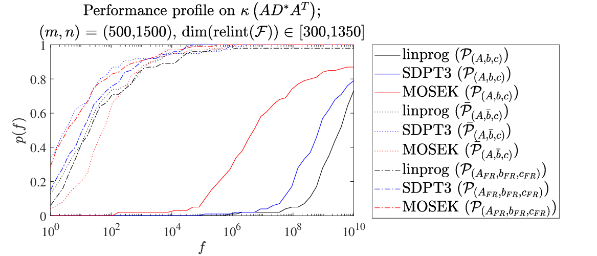
In Figure 4.1 we use a performance profile [20, 32] to observe the overall behaviour on different families of instances using the three solvers. The performance profile provides a useful graphical comparison for solver performances. Figure 4.1 displays the performance profile on the condition numbers of the normal matrix $AD^{*}A^{T}$ near optimal points from different solvers. We generate $100$ instances for each family that have $\dim(\relint({\mathcal{F}}))\in[300,1350]$ . The instance sizes are fixed with $(m,n)=(500,1500)$ . The vertical axis in Figure 4.1 represents the statistics of the performance ratio on $\kappa\left(AD^{*}A^{T}\right)$ , the condition number of normal matrix near optimum $(x^{*},s^{*})$ ; see equation 4.1. Roughly speaking, the vertical axis represents the probability of achieving a performance ratio within a factor of $f$ among all methods used. We used the lower the better statistics. The details of the performance ratio are discussed in [20, 32]. The solid lines in Figure 4.1 represent the performance of the instances $({\mathcal{P}}_{(A,b,c)})$ that fail strict feasibility. They show that the condition numbers of the normal matrices near optima are significantly higher when strict feasibility fails. That is, when strict feasibility fails for ${\mathcal{F}}$ , the matrix $AD^{*}A^{T}$ is more ill-conditioned and it is difficult to obtain search directions of high accuracy. We also observe that facially reduced instances yield smaller condition numbers near optima. We note that the instances $({\mathcal{P}}_{(A,b,c)})$ and $({\mathcal{P}}_{(A_{FR},b_{FR},c_{FR})})$ are equivalent.

4.1.3 Stopping Criteria

We now use the three solvers to observe the accuracy of the first-order optimality conditions (KKT conditions) and the running times, for the instances $({\mathcal{P}}_{(A,b,c)})$ and $({\mathcal{P}}_{(A_{FR},b_{FR},c_{FR})})$ , see Table 4.1. We test the average performance of $10$ instances of the size $(n,m,r)=(3000,500,2000)$ . The headers used in Table 4.1 provide the following. Given solver outputs $(x^{*},y^{*},s^{*})$ , the header ‘KKT’ exhibits the average of the triple consisting of the primal feasibility, dual feasibility and complementarity;

\text{KKT}=\left(\frac{\|Ax^{*}-b\|}{1+\|b\|},\ \frac{\|A^{T}y^{*}+s^{*}-c\|}{1+\|c\|},\ \frac{\langle x^{*},s^{*}\rangle}{n}\right).

The headers ‘iter’ and ‘time’ in Table 4.1 refer to the average of the number of iterations and the running time in seconds, respectively.

		Non-Facially Reduced System	Facially Reduced System
linprog	KKT	(2.44e-15, 2.05e-12, 3.18e-09)	(5.85e-16, 4.74e-16, 9.22e-09)
	iter	22.30	17.90
	time	2.34	0.81
SDPT3	KKT	(8.11e-10, 7.55e-12, 5.65e-02)	(1.43e-11, 3.67e-16, 4.38e-06)
	iter	25.50	19.30
	time	1.73	0.70
mosek	KKT	(7.52e-09, 1.80e-15, 3.27e-06)	(3.85e-09, 3.69e-16, 1.19e-06)
	iter	40.30	10.20
	time	1.40	0.35

Table 4.1: Average of KKT conditions, iterations and time of (non)-facially reduced problems

From Table 4.1 we observe that facially reduced instances provide significant improvement in first-order optimality conditions, the number of iterations and the running times for all solvers in general. We note that the instances $({\mathcal{P}}_{(A,b,c)})$ and $({\mathcal{P}}_{(A_{FR},b_{FR},c_{FR})})$ are equivalent. Hence, our empirics show that performing facial reduction as a preprocessing step not only improves the solver running time but also the quality of solutions.

4.1.4 Distance to Infeasibility

In this section we present empirics that illustrate the effect of perturbations of the right-hand side $b$ when strict feasibility fails. We recall, from 3.14, that there exists an arbitrarily small perturbation of the right-hand side vector $b$ of ${\mathcal{F}}$ that renders the set ${\mathcal{F}}$ infeasible, i.e., $\dist(b,{\mathcal{F}}=\emptyset)=0$ . Moreover, the vector $\Delta b=y$ that satisfies the auxiliary system equation 2.3 is a perturbation that makes the set ${\mathcal{F}}$ empty; see equation 3.9.

We follow the steps in Section 4.1.1 to generate instances of the order $(n,m)=(1000,200)$ and $r=\relint({\mathcal{F}})=900$ . The objective function $c^{T}x$ is chosen as presented in Section 4.1.1. For the fixed $(n,m,r)$ , we generate $10$ instances and observe the average performance of these instances as we gradually increase the magnitude of the perturbation. We recall the matrix $AV$ from equation 2.5. We use two types of perturbations for $b$ ;

\Delta b,\text{ where }\Delta b\in\range(AV)^{\perp},\quad\Delta\bar{b},\text{ where }\Delta\bar{b}\in\range(AV).

We choose $\Delta b$ to be the vector $y$ that satisfies equation 2.3. For $\Delta\bar{b}$ , we choose $AVd$ , where $d\in\mathbb{R}^{r}$ is a randomly chosen vector. As we increase $\epsilon>0$ , we observe the performance of the two families of the systems

\begin{array}[]{lll}Ax=b_{\epsilon}:=b-\epsilon\Delta b\ \text{ and }\ Ax=\bar{b}_{\epsilon}:=b-\epsilon\Delta\bar{b}.\end{array}

We use the interior point method from MATLAB’s linprog for the test. Figure 4.2 contains the average of the first-order optimality conditions evaluated at the solver outputs $(x^{*},y^{*},s^{*})$ of these instances; primal feasibility, dual feasibility and the complementarity.

The horizontal axis of Figure 4.2 indicates the degree of the perturbation imposed on the right-hand side vector $b$ , $\epsilon\|\Delta b\|$ and $\epsilon\|\Delta\bar{b}\|$ . The vertical axis indicates the individual component of the first-order optimality. From Figure 4.2, we observe that the KKT conditions with the perturbation $\Delta\bar{b}$ display a steady performance regardless of the perturbation degree; see the markers $\circ$ , $\square,\triangle$ with the dotted lines. In contrast, the markers $\bullet$ , $\blacksquare,\blacktriangle$ in Figure 4.2 exhibit the performance of the instances that are perturbed with $\Delta b$ and they display a different performance. In particular, we see that the relative primal feasibility $\|Ax^{*}-b_{\epsilon}\|/(1+\|b_{\epsilon}\|)$ , marked with $\bullet$ , consistently increases as the perturbation magnitude $\epsilon\|\Delta b\|$ increases when strict feasibility fails for ${\mathcal{F}}$ .

4.1.5 Empirics on Singular Values and $\ips$

In this section we present our numerical experiment on the ill-conditioning discussed in Section 3.3.4 in terms of $\maxsd$ (see Definition 2.5). We generated instances with different settings for $\maxsd=1,5$ and $10$ . We recall the generation for the vector $y$ and $A_{2}$ in Section 4.1.1. For generating and instance with $\maxsd>1$ , we generated $Y_{c}=\blkdiag(y^{1},\ldots,y^{\ips})\in\mathbb{R}^{m\times\maxsd}$ and $A_{2}=\blkdiag(A_{2}^{1},\ldots,A_{2}^{\maxsd})$ of appropriate dimension in order to produce the exposing vector $A_{2}^{T}\sum_{j=1}^{\maxsd}Y_{c}(:,j)\geq 0$ . Each column of $Y_{c}$ serves as a vector satisfying equation 2.3.

Let $\sigma_{\max}(AD^{*}A^{T})$ be the maximum singular value of $AD^{*}A^{T}$ . We count the number of singular values of $AD^{*}A^{T}$ that are smaller than $10^{-8}\cdot\sigma_{\max}(AD^{*}A^{T})$ . In Table 4.2 below, we report the cardinality of

{\@index{\@indexphrase{$\Sigma_{0}:=\{i:\sigma_{i}(AD^{*}A^{T})<\sigma_{\max}(AD^{*}A^{T})\}$}}}\ignorespaces\textit{$\Sigma_{0}:=\{i:\sigma_{i}(AD^{*}A^{T})<\sigma_{\max}(AD^{*}A^{T})\}$}.

We test the average performance on the $20$ instances of the fixed size $(n,m,r)=(3000,500,2000)$ . We display the average number of $|\Sigma_{0}|$ . We see from Table 4.2

		$\maxsd$ = 1	$\maxsd$ = 5	$\maxsd$ = 10
linprog	$\|\Sigma_{0}\|$	4.10	8.65	13.10
SDPT3	$\|\Sigma_{0}\|$	4.75	8.00	34.65
MOSEK	$\|\Sigma_{0}\|$	6.45	12.35	14.50

Table 4.2:

\#

(rel.) small singular values of

AD^{*}A^{T}

near optimum; average over

20

instances

a larger $\maxsd$ and $\ips$ values produce a greater number of small singular values. When there is a significant number of redundant constraints, it is more difficult to obtain a good search direction due to a large number of relatively small singular values.

4.2 Empirics with Simplex Method

In this section we compare the behaviour of the dual simplex method with instances that have strictly feasible points and instances that do not. We also observe the degeneracy issues that arise in the instances from NETLIB.

4.2.1 Empirics on the Number of Degenerate Iterations

In this section we test how the lack of strict feasibility affects the performance of the dual simplex method. We provide the construction of instances that fail strict feasibility in Section A.3.2. We choose MOSEK for our tests since MOSEK reports the percentage of degenerate iterations as a part of the solver report. MOSEK reports the quantity ‘DEGITER( $\%$ )’, the ratio of degenerate iterations.

Given a set ${\mathcal{G}}$ and a point $(y,s)\in\relint({\mathcal{G}})\subseteq\mathbb{R}^{m}\oplus\mathbb{R}^{n}_{+}$ , let $r$ be the number of positive entries of $s$ , i.e., $r=|\supp(s)|$ . In our tests, we gradually increase $r$ for fixed $n,m$ and generate instances for ${\mathcal{G}}$ as described in Section A.3.2. We then observe the behaviour of the dual simplex method. Table 4.3 contains the results. In Table 4.3, a smaller value for the header $(r/n)\%$ means that there are more entries of $s$ that are identically $0$ in the set ${\mathcal{G}}$ ; and the value $0\%$ means that strict feasibility holds. For each triple $(n,m,r)$ , we generated $10$ instances and we report the average of ‘DEGITER( $\%$ )’ of these instances.

		$100\%-(r/n)\%$
		40	30	20	10	0
$(n,m)$	(1000, 250)	36.62	10.18	0.01	0.02	0.00
	(2000, 500)	39.72	18.28	0.07	0.15	0.01
	(3000, 750)	25.99	10.66	0.32	0.75	0.02
	(4000, 1000)	29.78	18.25	0.25	0.53	0.02

Table 4.3: Average of the ratio of degenerate iterations

We recall Theorem 3.1: lack of strict feasibility implies that all basic feasible solutions are degenerate. However, we observe more, i.e., from Table 4.3, the frequency of degenerate iterations increases as $r$ decreases. In other words, higher degeneracy of the set ${\mathcal{G}}$ yields more degenerate iterations when the dual simplex method is used.

4.2.2 NETLIB Problems; Perturbations; Stability

We now illustrate the lack of strict feasibility on instances from the NETLIB data set. We used the following first $67$ instances that are in standard form at this link:

25fv47	adlittle^∗	afiro	agg^∗	agg2^∗	agg3^∗	bandm^∗	beaconfd^∗	blend	bnl1^∗
bnl2^∗	brandy^∗	cre $\_$ a^∗	cre $\_$ b^∗	cre $\_$ c^∗	cre $\_$ d^∗	d2q06c^∗	degen2^∗	degen3^∗	e226^∗
fffff800^∗	israel	lotfi	maros $\_$ r7	nug05	nug06	nug07	nug08	nug12	nug15
nug20	osa $\_$ 07^∗	osa $\_$ 14^∗	qap12	qap15	qap8	sc105^∗	sc205^∗	sc50a^∗	sc50b^∗
scagr25	scagr7	scfxm1^∗	scfxm2^∗	scfxm3^∗	scorpion^∗	scrs8^∗	scsd1	scsd6	scsd8
sctap1	sctap2	sctap3	share1b	share2b	ship04l^∗	ship04s^∗	ship08l^∗	ship08s^∗	ship12l^∗
ship12s^∗	stocfor1	stocfor2	stocfor3	truss	wood1p^∗	woodw^∗

We removed redundant rows to guarantee full row rank of $A$ .

Surprisingly, the Slater condition fails for $37$ out of these $67$ instances.¹³¹³ 13 The instances that fail strict feasibility are marked with an asterisk $*$ in the list above. This has interesting implications for both interior point and simplex methods. The standard interior point method stopping criteria is complicated by the unbounded dual optimal set. For the primal simplex method, every iteration is at a degenerate BFS and stalling generally occurs. Therefore preprocessing to eliminate the variables fixed at $0$ is important. In addition, in order to motivate robust optimization, it is shown in e.g., [3, 4] that optimal solutions of many of the NETLIB instances are extremely sensitive to perturbations in the data. We now see this to be the case, and we show that FR regularizes the problem and avoids this instability.

We first use the instance degen3 in order to illustrate the consequence of lack of strict feasibility. The data matrix $A$ after removing two redundant rows is $1501$ -by- $2604$ . After FR, we obtain the constraint matrix $P_{\bar{m}}AV$ of size $1226$ -by- $1648$ . This implies that $2604-1648=956$ number of variables are identically $0$ on the feasible set. Furthermore, $\ips({\mathcal{F}})=275$ equality constraints are implicitly redundant. By Item 3 of 3.9, without FR, the degree of degeneracy of every BFS is at least $275$ . Namely, the length of the basis is $1501$ and every basis contains at least $275$ degenerate indices.

We now illustrate that FR gives a more robust model with respect to data perturbations using the instance brandy. Let $(A,b)$ be the data after removing the redundant equality constraints. Let $(P_{\bar{m}}AV,P_{\bar{m}}b)$ be the data for the facially reduced system. The data matrices $A$ and $P_{\bar{m}}AV$ have sizes $193$ -by- $303$ and $155$ -by- $260$ , respectively¹⁴¹⁴ 14 This also means that, without FR, every BFS has at least $38$ degenerate basic variables. At least $19.69$ percent of basic variables are always degenerate.. Set the perturbation scalars $\epsilon_{A}=\epsilon_{b}=10^{-9}$ . We construct a random perturbation matrix $\Phi,\|\Phi\|_{F}=\|A\|_{F}+1$ , and random perturbation vector $\phi,\|\phi\|_{2}=\|b\|_{2}+1$ . We then solve the problem

\tilde{p}^{*}=\max\{\langle c,x\rangle:(A+\epsilon_{A}\Phi)x=b+\epsilon_{b}\phi,\ x\geq 0\}.

For the facially reduced system, we used the identical perturbation data $\Phi,\phi$ and discard the rows and columns of $(A,b)$ found from FR. That is, we use the perturbations $P_{\bar{m}}\Phi V$ and $P_{\bar{m}}\phi$ to the facially reduced system after the scaling $\|P_{\bar{m}}\Phi V\|_{F}=\|P_{\bar{m}}AV\|_{F}+1$ and $\|P_{\bar{m}}\phi\|_{2}=\|P_{\bar{m}}b\|_{2}+1$ . We then solve

\max\{\langle V^{T}c,v\rangle:(P_{\bar{m}}AV+\epsilon_{A}P_{\bar{m}}\Phi V)v=P_{\bar{m}}b+\epsilon_{b}P_{\bar{m}}\phi,\ v\geq 0\}.

In this way, we maintain the identical perturbation structure for the original system and the facially reduced system. We also generate a transportation problem and use the aforementioned perturbations. We note that the transportation problems have Slater points but are known to be highly degenerate. The size of the data generated is $49$ -by- $600$ .

In the experiment, we tested the instances using $100$ different perturbation settings. We randomly generated perturbations $\Phi,\phi$ with density set at $0.1$ . We used MOSEK simplex with the setting ‘MSK $\_$ OPTIMIZER $\_$ FREE $\_$ SIMPLEX’. In Table 4.4, the headers $\epsilon_{A}$ and $\epsilon_{b}$ refer to the scalars used for perturbations as described above. The headers $(A,b)$ , $(P_{\bar{m}}AV,P_{\bar{m}}b)$ and $(A_{\text{trans}},b_{\text{trans}})$ refer to the non-facially reduced system, the facially reduced system and the transportation problems, with the perturbations. The integral values in the table indicate the number of times that the solver outputs PRIMAL $\_$ AND $\_$ DUAL $\_$ FEASIBLE. Let $p^{*}$ be the optimal value for the unperturbed instance brandy, and let $\tilde{p}^{*}$ be the optimal value of a perturbed instance of brandy. The non-integral values in the table indicate the average relative difference in the optimal values between $p^{*}$ and $\tilde{p}^{*}$ . The relative difference is computed using the formula $\frac{|p^{*}-\tilde{p}^{*}|}{2|p^{*}+\tilde{p}^{*}|}$ . For example, the first entry $11$ in Table 4.4 means that $100\!-\!11$ out of $100$ perturbed instances yield infeasibility or unknown status, i.e., only $11$ solved successfully. The entry 4.938e-02 next to $11$ indicates the average of $\frac{|p^{*}-\tilde{p}^{*}|}{2|p^{*}+\tilde{p}^{*}|}$ on those $11$ instances.

		$(A,b)$	$(P_{\bar{m}}AV,P_{\bar{m}}b)$	$(A_{\text{trans}},b_{\text{trans}})$
1.0e-09	0	( 11 , 4.938e-02 )	( 97 , 6.705e-03 )	100
0	1.0e-09	( 27 , 2.470e-10 )	( 100 , 2.208e-10 )	100
1.0e-09	1.0e-09	( 11 , 1.339e-01 )	( 96 , 8.719e-03 )	100

Table 4.4: Number of successful results out of

100

perturbed instances using simplex method on the instance brandy and transportation problem

The columns $(A,b)$ and $(P_{\bar{m}}AV,P_{\bar{m}}b)$ in Table 4.4 demonstrate that the facially reduced problems are more immune to data perturbations; the number of successfully solved perturbed instances are significantly larger and the optimal values under the perturbations are less influenced. The last column indicates that although the instance may have many degenerate BFSs, having a strictly feasible point is important in terms of perturbations in data, i.e., this emphasizes the difference between the two types of degeneracy.

5 Conclusion

We have addressed the impact, for both theoretical and computational reasons, of loss of strict feasibility in LP, distinguishing one type of degeneracy at a BFS. For our numerics we illustrated this using the accuracy of optimality conditions as well as the effect of perturbations, for the two most popular classes of algorithms, i.e., simplex and interior point methods. For the theory, we proved, using the two-step facial reduction, that if strict feasibility fails for a linear program, then every BFS is degenerate. In addition, we showed that facial reduction can be implemented efficiently to obtain a smaller simpler problem with strict feasibility, and that this improves stability. This was illustrated on random problems, as well as instances from the NETLIB data set.

An essential step for almost all algorithms for linear programming is preprocessing. One part of preprocessing is identifying fixed variables. However, identifying variables fixed at $0$ , facial reduction, has not been done due to expense and accuracy problems. In this paper we have shown that not eliminating these variables, i.e., lack of strict feasibility, is equivalent to implicit singularity and this helps explain the numerical difficulties that arise. We have further provided an efficient preprocessing step for facial reduction, i.e., we continue on phase I of the simplex method that eliminates all the artificial variables, and eliminate the variables fixed at $0$ . We observed that a variable that is basic (positive) in every BFS corresponds to a redundant constraint and, by complementary slackness, corresponds to a variable fixed at $0$ in the dual. And redundant constraints have been shown in the literature to poorly affect algorithms [18]. Moreover, identifying redundant constraints is a nontrivial operation e.g., [10]. This motivates doing FR on both the primal and the dual problems. (It is still unclear whether or not we have to repeat FR on the primal again.)

In the literature, in particular in textbooks on LP, the method most often used to handle a free variable $x_{i}$ is to replace it by two nonnegative variables $x_{i}\leftarrow x_{i}^{+}-x_{i}^{-}$ . The means that the optimal solution is unbounded as one can add an arbitrary positive constant to both new variables. But then strict feasibility fails for the dual, i.e., stable problems are transformed into ill-conditioned problems. One can speculate that this may account for the large number of instances in the NETLIB set where strict feasibility fails and numerical accuracy is difficult to maintain.

We have presented various numerical experiments that convey the importance of preprocessing for strict feasibility for linear programs, Section 4. For interior point methods, we illustrated the importance of strict feasibility using condition numbers and relationships with nearness to infeasibility. We also shed light on the main difficulties that arose with the implicit redundant constraints and used the QR decomposition to show how these difficulties come into play. This also relates to the implicit problem singularity, $\ips$ . A larger $\ips$ means that there is a higher chance of inducing an infeasible problem under perturbations. A large number of degenerate BFSs is believed to cause difficulties for the simplex method. We have shown that the settings for having many identically $0$ variables in the dual program yield many degenerate iterations in the simplex method. We also have shown that many NETLIB instances fail strict feasibility and used selected instances to show the effect of this degeneracy. Moreover, the facially reduced problems are seen to be more robust with respect to data perturbations. In addition, an essential element of solving an LP is postoptimal analysis, this becomes difficult when strict feasibility fails and perturbations of $b$ can lead to infeasibility. These facts further emphasize that ensuring strict feasibility should be part of preprocessing for linear programming.

Our results can easily extend to other forms of LPs and to more general problems where degeneracies arise, such as the active set method for quadratic programs [51, 23]. We are currently extending the efficient FR technique to semidefinite programs.

Acknowledgements

This research is supported by the National Sciences and Engineering Research Council (NSERC) of Canada, Grant $\#$ No. 50503-10827.

Appendix A Technical Proofs, Supplementary Materials

A.1 proof of 3.2

Proof.

Let $x\in F$ and let $r$ be the number of positive entries in $x$ . Let $\bar{x}\in\mathbb{R}^{r}$ be the vector obtained by discarding the $0$ entries in $x$ . This is readily given by the following matrix-vector multiplication $\bar{x}=I(\supp(x),:)x$ , where $\supp(x)$ is the support of $x$ , the set of indices $\{i:x_{i}>0\}$ . Let $\bar{A}\in\mathbb{R}^{m\times r}$ be the matrix after removing the columns of $A$ that are not in the support of $x$ , i.e., $\bar{A}=A_{\supp(x)}$ . We note that $\bar{x}$ is a particular solution to the system $\bar{A}z=b$ and $\bar{x}>0$ .

Suppose to the contrary that $r>m+d$ . Since $r-m>d$ , there exists at least $d+1$ linearly independent vectors, say $v_{1},\ldots,v_{d+1}\in\mathbb{R}^{r}$ , satisfying $\bar{A}v_{i}=0,\ \forall i=1,\ldots,d+1$ . For each $i\in\{1,\ldots,d+1\}$ and for $\epsilon\in\mathbb{R}$ , we define

\begin{array}[]{ll}v_{i,+}:=\bar{x}+\epsilon v_{i},&v_{i,-}:=\bar{x}-\epsilon v_{i},\\ x_{i,+}:=I(:,\supp(x))\left(\bar{x}+\epsilon v_{i}\right),&x_{i,-}:=I(:,\supp(x))\left(\bar{x}-\epsilon v_{i}\right).\\ \end{array}

For a sufficiently small $\epsilon$ , we have $x_{i,+},x_{i,-}\in{\mathcal{F}}$ . We note that $x=\frac{1}{2}(x_{i,+}+x_{i,-}),\ \forall i$ . Hence, by the definition of face, $x_{i,+}\in F,\ \forall i$ . Therefore, $F$ contains vectors $\{x_{i,+}\}_{i=1,\ldots,d+1}\cup\{x\}$ that are affinely independent and hence $\dim(F)\geq d+1$ . ∎

A.2 A Condition Measure using Degeneracy

Although degeneracy is a well-known subject, to the best of our knowledge, the relationships between degeneracy and stability are rarely discussed. We now show that the degree of degeneracy at a BFS provides useful information on the robustness of the LP; the least degenerate BFS provides an upper bound on the number of implicitly redundant equalities of the set ${\mathcal{F}}$ . We note that an ${\mathcal{F}}$ that contains a large number of implicit redundancies is a more ill-conditioned set. (This is comparable to a linear system $Ax=b$ with more redundant rows having the error in the solution being more susceptible to perturbations of $b$ .)

The arguments used in the proof of 3.9 are rather algebraic. The geometric argument used in the proof of 3.4 provides two useful estimates. For any extreme point $x\in{\mathcal{F}}$ , the number of nonzero elements of $x$ , $|\supp(x)|$ , satisfies

|\supp(x)|\leq m-\ips({\mathcal{F}})\implies\ips({\mathcal{F}})\leq m-|\supp(x)|.

Since this holds for all extreme points of ${\mathcal{F}}$ , we get the following:

\sd({\mathcal{F}})\leq\maxsd({\mathcal{F}})\leq\ips({\mathcal{F}})\leq\ \hat{d}:=\min_{\text{{BFS}\,$x\in{\mathcal{F}}$}}\ \{\text{degree of degeneracy of $x$}\}.

(A.1)

The shortest FR steps for ${\mathcal{F}}$ , $\sd({\mathcal{F}})$ , is at most $1$ , thus the inequality $\sd({\mathcal{F}})\leq\hat{d}$ does not provide useful information. However, the relation (A.1) provides two meaningful corollaries related to $\maxsd({\mathcal{F}})$ and $\ips({\mathcal{F}})$ :

1.

The inequality $\maxsd({\mathcal{F}})\leq\hat{d}$ implies that the number of nontrivial FR steps cannot exceed the degree of degeneracy of a least degenerate BFS of ${\mathcal{F}}$ ;
2.

The inequality $\ips({\mathcal{F}})\leq\hat{d}$ shows that it is useful to record the minimum degree of degeneracy observed throughout the simplex iterations. This gives an estimate for the number of implicitly redundant equalities of ${\mathcal{F}}$ .

If ${\mathcal{F}}$ contains a nondegenerate BFS, we get $\hat{d}=0$ . Hence $\sd({\mathcal{F}})=\maxsd({\mathcal{F}})=\ips({\mathcal{F}})=0$ and it provides an alternative way to view 3.6. We comment that evaluating and recording the degree of degeneracy of a BFS are not expensive operations.

A.3 Dual Degeneracy in the Absence of Strict Feasibility

A.3.1 Implicit Redundancies in the Dual

The following Lemma A.1 provides the corresponding dual form of the theorem of the alternative for set ${\mathcal{G}}$ in equation 3.14.

Lemma A.1 (theorem of the alternative in dual form, [13, Theorem 3.3.10]).

Let ${\mathcal{G}}\neq\emptyset$ in equation 3.14. Then, exactly one of the following statements holds:

1.

There exists $(y,s)\in\mathbb{R}^{m}\oplus\mathbb{R}_{++}^{n}$ with $A^{T}y+s=c$ , i.e., strict feasibility holds for ${\mathcal{G}}$ ;
2.

There exists $w\in\mathbb{R}^{n}$ such that

$0\neq w\in\mathbb{R}_{+}^{n},\ Aw=0\ \text{ and }\ \langle c,w\rangle=0.$ (A.2)

We recall that the vector $A^{T}y$ in equation 2.4 provides an exposing vector to the set ${\mathcal{F}}$ . Similarly, a solution $w$ to the auxiliary system equation A.2 provides an exposing vector for ${\mathcal{G}}$ :

(y,s)\in{\mathcal{G}}\,\implies\,\left\{\langle w,s\rangle=\langle w,c-A^{T}y\rangle=\langle c,w\rangle-\langle Aw,y\rangle=0-\langle 0,y\rangle=0\right\}.

We let

{\mathcal{I}}_{w}=\{1,\ldots,n\}\setminus\supp(w),\ U=I(:,{\mathcal{I}}_{w})\ \text{ and }\ s_{w}=|\supp(w)|.

Then, the facially reduced system of ${\mathcal{G}}$ is given by

\left\{(y,u)\in\mathbb{R}^{m}\oplus\mathbb{R}_{+}^{n-s_{w}}\ :\ \begin{bmatrix}A^{T}&U\end{bmatrix}\begin{pmatrix}y\\ u\end{pmatrix}=c\right\}.

(A.3)

The notion of degeneracy in Section 2.1 naturally extends to an arbitrary polyhedron, e.g., see [5, Section 2]. For a general polyhedron $P\subseteq\mathbb{R}^{n}$ , a point $p$ in $P$ is called a basic solution if there are $n$ linearly independent active constraints at $p$ . In addition, if there are more than $n$ active constraints at the point $p\in P$ , then the point $p$ is called degenerate. Using this definition of degeneracy, we now show that the absence of strict feasibility for ${\mathcal{G}}$ implies that every basic feasible solution of ${\mathcal{G}}$ is degenerate.

First, note that the facially reduced system in equation A.3 contains a redundant constraint, i.e., let $w$ be an exposing vector for ${\mathcal{G}}$ from the system equation A.2. Then we have

\begin{bmatrix}A\\ U^{T}\end{bmatrix}w=\begin{bmatrix}Aw\\ U^{T}w\end{bmatrix}=\begin{bmatrix}0_{m}\\ 0_{n-s_{w}}\end{bmatrix}.

In other words, there is a nontrivial row combination of $\begin{bmatrix}A^{T}&U\end{bmatrix}$ that yields the $0$ vector implying the existence of a redundant row and a redundant constraint in the facially reduced system. The redundancy immediately implies the dual degeneracy; for any basic solution of ${\mathcal{G}}$ , there always exists an redundant equality in $\begin{bmatrix}A^{T}&I\end{bmatrix}\begin{pmatrix}y\\ s\end{pmatrix}=c$ .

A.3.2 Construction of Dual LPs without Strict Feasibility

We first show how to generate an instance for the dual feasible set ${\mathcal{G}}$ that fails strict feasibility. The construction is similar to the one in Section 4.1.1. We generate a degenerate problem by finding a feasible auxiliary system equation A.2. Given $m,n,r\in\mathbb{N}$ , we construct $A\in\mathbb{R}^{m\times n}$ and $c\in\mathbb{R}^{n}$ that satisfy equation A.2 with $\dim(\relint({\mathcal{G}}))=m+r$ .

1.

Pick any $0\neq w\in\mathbb{R}_{+}^{n}$ with $|\supp(w)|=n-r$ . Let

$\{w\}^{\perp}=\spann\{d_{i}\}_{i=1}^{n-1}\subset\mathbb{R}^{n}\quad\left(=\nul(w^{T})\right).$

We let $D\in\mathbb{R}^{(n-1)\times n}$ be the matrix where its rows consist of $\{d_{i}^{T}\}_{i=1}^{n-1}$ . We let $R\in\mathbb{R}^{m\times(n-1)}$ be a random matrix and we set $A=RD$ . We note that $Aw=0$ .
2.

Pick $s\in\mathbb{R}_{+}^{n}$ so that

$s_{i}=\left\{\begin{array}[]{ll}0&\text{if }i\in\supp(w)\\ \text{positive }&\text{if }i\notin\supp(w).\end{array}\right.$

We note that $\langle w,s\rangle=0$ holds.
3.

Pick $y\in\mathbb{R}^{m}$ and set $c=A^{T}y+s$ . We note that $\langle c,w\rangle=0$ holds.

For the empirics, we construct the objective function $b^{T}y$ of $({\mathcal{D}})$ by choosing a vector $\hat{x}\in\mathbb{R}_{++}^{n}$ and setting $b=A\hat{x}$ .

Index

( ${\mathcal{D}}$ ), dual of ( ${\mathcal{P}}$ ) §A.3.1, §3.3.2
$({\mathcal{P}})$ §2.1
$A_{\mathcal{I}}$ , submatrix of $A$ with columns in ${\mathcal{I}}$ §2.1
${\mathcal{B}}_{0}$ §3.2.2
basic feasible solution, BFS §2.1.1
basic solution §A.3.1
BFS , basic feasible solution §2.1.1
degenerate §A.3.1
degenerate BFS §2.1.1
degree of degeneracy §3.1.3, §3.2.2, §4.2.2
distance to infeasibility §2.2, §3.3.1
distance to infeasibility, $\dist(b,{\mathcal{F}}=\emptyset)$ §3.3.1
dual feasible set, ${\mathcal{G}}$ §A.3.1
dual of ( ${\mathcal{P}}$ ), ( ${\mathcal{D}}$ ) §A.3.1, §3.3.2
exposing vector §2.2
extreme point §3.1.2
${\mathcal{F}}$ , feasible region §2.1
face §2.2, §3.1.2
facial range vector §2.2
facial reduction, FR §1, §2.2
feasible region, ${\mathcal{F}}$ §2.1
fixed at $0$ §2.1.1, §2.2
FR, facial reduction §1
${\mathcal{G}}$ , dual feasible set §A.3.1
${\mathcal{I}}_{+}=\{1,\ldots,n\}\backslash{\mathcal{I}}_{0}$ §2.1.1
$I$ , the identity matrix §2.2
${\mathcal{I}}_{0}$ §3.1.3, §3.2.2
${\mathcal{I}}_{0}:=\{i\,:\,x_{i}=0,\forall x\in{\mathcal{F}}\}$ §2.1.1
implicit problem singularity, $\ips({\mathcal{S}})=m-m_{r}$ Definition 2.5
$\ips$ §3.1.3
$\ips({\mathcal{S}})=m-m_{r}$ , implicit problem singularity §2.2
largest number nontrivial facial reduction steps, $\maxsd({\mathcal{S}})$ §2.2
linear program, LP §1
linprog §4
LP, linear program §1
Mangasarian-Fromovitz §1
max-singularity degree Definition 2.5
$\maxsd$ §3.1.3
$\maxsd({\mathcal{S}})$ , largest number nontrivial facial reduction steps §2.2
minimal face §2.2
MOSEK §4
nondegenerate BFS §2.1.1
nonnegative orthant, $\mathbb{R}_{+}^{n}$ §2.1
performance profile §4.1.2
positive orthant, $\mathbb{R}_{++}^{n}$ §2.1
postoptimal analysis §5
$P_{\bar{m}}:\mathbb{R}^{m}\to\mathbb{R}^{\bar{m}}$ §2.2
$P_{\bar{m}}AV$ §2.2, §3.1.2, §4.2.2
$P_{\bar{m}}b$ §2.2, §3.1.2, §4.2.2
$p^{*}$ §2.1
$\mathbb{R}_{++}^{n}$ , positive orthant §2.1
$\mathbb{R}_{+}^{n}$ , nonnegative orthant §2.1
real vector space of $m$ -by- $n$ matrices, $\mathbb{R}^{m\times n}$ §2.1
relative interior, $\relint$ §2.1, §3.3.2
$\mathbb{R}^{m\times n}$ , real vector space of $m$ -by- $n$ matrices §2.1
SDPT3 §4
singularity degree, $\sd({\mathcal{S}})$ Definition 2.4
Slater condition §1
stalling §1, §4.2.2
$\supp$ §2.1
$\supp$ , support §A.1
support of exposing vector for ${\mathcal{F}}$ , $s_{z}$ §2.2
support of exposing vector for ${\mathcal{G}}$ , $s_{w}$ §A.3.1
support, $\supp$ §A.1
$s_{w}$ , support of exposing vector for ${\mathcal{G}}$ §A.3.1
$s_{z}$ , support of exposing vector for ${\mathcal{F}}$ §2.2
$\{1,\ldots,n\}$ §2.1.1
$\dist(b,{\mathcal{F}}=\emptyset)$ , distance to infeasibility §3.3.1
$\relint$ , relative interior §2.1, §3.3.2
$\bar{m}={\rank(AV)}$ §2.2
$\Sigma_{0}:=\{i:\sigma_{i}(AD^{*}A^{T})<\sigma_{\max}(AD^{*}A^{T})\}$ §4.1.5
$\langle\cdot,\cdot\rangle$ , inner product §2.1

References

[1] E.D. Andersen. Finding all linearly dependent rows in large-scale linear programming. Optimization methods & software, 6(3):219–227, 1995.
[2] E.D. Andersen and K.D. Andersen. Presolving in linear programming. mprog, 71(2):221–245, 1995.
[3] A. Ben-Tal, L. El Ghaoui, and A. Nemirovski. Robust optimization. Princeton Series in Applied Mathematics. Princeton University Press, Princeton, NJ, 2009.
[4] A. Ben-Tal and A. Nemirovski. Robust solutions of uncertain linear programs. Oper. Res. Lett., 25(1):1–13, 1999.
[5] D. Bertsimas and J. Tsitsiklis. Introduction to Linear Optimization. Athena Scientific, Belmont, MA, 1997.
[6] R.E. Bixby. Solving real-world linear programs: a decade and more of progress. Oper. Res., 50(1):3–15, 2002. 50th anniversary issue of Operations Research.
[7] Robert G. Bland. New finite pivoting rules for the simplex method. Math. Oper. Res., 2(2):103–107, 1977.
[8] J.M. Borwein and H. Wolkowicz. Facial reduction for a cone-convex programming problem. J. Austral. Math. Soc. Ser. A, 30(3):369–380, 1980/81.
[9] J.M. Borwein and H. Wolkowicz. Regularizing the abstract convex program. J. Math. Anal. Appl., 83(2):495–530, 1981.
[10] R.J. Caron, A. Boneh, and S. Boneh. Redundancy. In Advances in sensitivity analysis and parametric programming, volume 6 of Internat. Ser. Oper. Res. Management Sci., pages 13.1–13.41. Kluwer Acad. Publ., Boston, MA, 1997.
[11] R. Chandrasekaran, Santosh N. Kabadi, and Katta G. Murty. Some NP-complete problems in linear programming. Oper. Res. Lett., 1(3):101–104, 1981/82.
[12] A. Charnes. Optimality and degeneracy in linear programming. Econometrica, 20:160–170, 1952.
[13] Y.-L. Cheung. Preprocessing and Reduction for Semidefinite Programming via Facial Reduction: Theory and Practice. PhD thesis, University of Waterloo, 2013.
[14] Y-L. Cheung, S. Schurr, and H. Wolkowicz. Preprocessing and regularization for degenerate semidefinite programs. In D.H. Bailey, H.H. Bauschke, P. Borwein, F. Garvan, M. Thera, J. Vanderwerff, and H. Wolkowicz, editors, Computational and Analytical Mathematics, In Honor of Jonathan Borwein’s 60th Birthday, volume 50 of Springer Proceedings in Mathematics & Statistics, pages 225–276. Springer, 2013.
[15] V. Chvátal. Linear programming. A Series of Books in the Mathematical Sciences. W. H. Freeman and Company, New York, 1983.
[16] G.B. Dantzig. Linear Programming and Extensions. Princeton University Press, Princeton, New Jersey, 1963.
[17] G.B. Dantzig, A. ORDEN, and P. WOLFE. The generalized simplex method for minimizing a linear form under linear inequality restraints. Pacific J. Math., 5:183–195, 1955.
[18] A. Deza, E. Nematollahi, R. Peyghami, and T. Terlaky. The central path visits all the vertices of the Klee-Minty cube. Optim. Methods Softw., 21(5):851–865, 2006.
[19] A. Deza, E. Nematollahi, and T. Terlaky. How good are interior point methods? Klee-Minty cubes tighten iteration-complexity bounds. Math. Program., 113(1, Ser. A):1–14, 2008.
[20] E.D. Dolan and J.J. Moré. Benchmarking optimization software with performance profiles. Math. Program., 91(2, Ser. A):201–213, 2002.
[21] D. Drusvyatskiy, G. Li, and H. Wolkowicz. A note on alternating projections for ill-posed semidefinite feasibility problems. Math. Program., 162(1-2, Ser. A):537–548, 2017.
[22] D. Drusvyatskiy and H. Wolkowicz. The many faces of degeneracy in conic optimization. Foundations and Trends^® in Optimization, 3(2):77–170, 2017.
[23] A. Forsgren, P.E. Gill, and E. Wong. Primal and dual active-set methods for convex quadratic programming. Mathematical programming, 159(1-2):469–508, 2015.
[24] R.M. Freund and F. Ordonez. On an extension of condition number theory to nonconic convex optimization. Mathematics of operations research, 30(1):173–194, 2005.
[25] R.M. Freund and J.R. Vera. Some characterizations and properties of the “distance to ill-posedness” and the condition measure of a conic linear system. Technical report, MIT, Cambridge, MA, 1997.
[26] T. Gal, editor. Degeneracy in optimization problems. Baltzer Science Publishers BV, Bussum, 1993. Ann. Oper. Res. 46/47 (1993), no. 1-4.
[27] J. Gauvin. A necessary and sufficient regularity condition to have bounded multipliers in nonconvex programming. Mathematical programming, 12(1):136–138, 1977.
[28] J. Gauvin. Degeneracy, normality, stability in mathematical programming. In Recent developments in optimization (Dijon, 1994), volume 429 of Lecture Notes in Econom. and Math. Systems, pages 136–141. Springer, Berlin, 1995.
[29] A.J. Goldman and A.W. Tucker. Theory of linear programming. In Linear inequalities and related systems, pages 53–97. Princeton University Press, Princeton, N.J., 1956. Annals of Mathematics Studies, no. 38.
[30] J. Gondzio. Presolve analysis of linear programs prior to applying an interior point method. INFORMS J. Comput., 9(1):73–91, 1997.
[31] M. Gonzalez-Lima, H. Wei, and H. Wolkowicz. A stable primal-dual approach for linear programming under nondegeneracy assumptions. Comput. Optim. Appl., 44(2):213–247, 2009.
[32] Nicholas Gould and Jennifer Scott. A note on performance profiles for benchmarking software. ACM transactions on mathematical software, 43(2):1–5, 2016.
[33] O. GüLer, D. Den Hertog, C. Roos, T. Terlaky, and T. Tsuchiya. Degeneracy in interior point methods for linear programming: a survey. Ann. Oper. Res., 46/47(1-4):107–138, 1993. Degeneracy in optimization problems.
[34] J.A.J. Hall and K.I.M. McKinnon. The simplest examples where the simplex method cycles and conditions where EXPAND fails to prevent cycling. Math. Program., 100(1, Ser. B):133–150, 2004.
[35] X. Huang. Preprocessing and postprocessing in linear optimization. Master’s thesis, McMaster University, 2004.
[36] J. Im and H. Wolkowicz. A strengthened Barvinok-Pataki bound on SDP rank. Oper. Res. Lett., 49(6):837–841, 2021. 11 pages, accepted Aug. 2021.
[37] O. L. Mangasarian and S. Fromovitz. The Fritz John necessary optimality conditions in the presence of equality and inequality constraints. J. Math. Anal. Appl., 17:37–47, 1967.
[38] N. Megiddo. A note on degeneracy in linear programming. Math. Programming, 35(3):365–367, 1986.
[39] Cs. Mészáros and U.H. Suhl. Advanced preprocessing techniques for linear and quadratic programming. OR Spectrum, 25(4):575–595, 2003.
[40] C. Mészáros and U.H. Suhl. Advanced preprocessing techniques for linear and quadratic programming. OR Spectrum, 25:575–595, 2003. 10.1007/s00291-003-0130-x.
[41] G. Pataki. On the rank of extreme matrices in semidefinite programs and the multiplicity of optimal eigenvalues. mor, 23(2):339–358, 1998.
[42] F.N. Permenter. Reduction methods in semidefinite and conic optimization. PhD thesis, Massachusetts Institute of Technology, 2017.
[43] D.W. Peterson. A review of constraint qualifications in finite-dimensional spaces. SIAM Rev., 15:639–654, 1973.
[44] J. Renegar. Some perturbation theory for linear programming. Math. Programming, 65(1, Ser. A):73–91, 1994.
[45] D. M. Ryan and M. R. Osborne. On the solution of highly degenerate linear programmes. mprog, 41:385–392, 1988.
[46] L. Schork and J. Gondzio. Rank revealing Gaussian elimination by the maximum volume concept. Linear Algebra Appl., 592:1–19, 2020.
[47] S. Sremac. Error bounds and singularity degree in semidefinite programming. PhD thesis, University of Waterloo, 2019.
[48] S. Sremac, H.J. Woerdeman, and H. Wolkowicz. Error bounds and singularity degree in semidefinite programming. SIAM J. Optim., 31(1):812–836, 2021.
[49] J.F. Sturm. Error bounds for linear matrix inequalities. SIAM J. Optim., 10(4):1228–1248 (electronic), 2000.
[50] T. Terlaky and S.Z. Zhang. Pivot rules for linear programming: a survey on recent theoretical developments. Ann. Oper. Res., 46/47(1-4):203–233, 1993. Degeneracy in optimization problems.
[51] P. Wolfe. The simplex method for quadratic programming. Econometrica, 27(3):382–398, 1959.
[52] S. Wright. Primal-Dual Interior-Point Methods. Society for Industrial and Applied Mathematics (SIAM), Philadelphia, Pa, 1996.
[53] Y. YE, M.J. Todd, and S. MIZUNO. An ${\cal O}(\sqrt{n}L)$ –iteration homogeneous and self–dual linear programming algorithm. mor, 19:53–67, 1994.

Revisiting Degeneracy, Strict Feasibility, Stability, in Linear Programming

Abstract

1 Introduction

2 Preliminaries

2.1 Background and Notation

2.1.1 Degeneracy in LP

Remark 2.1.

2.2 Facial Reduction

Proposition 2.2.

Lemma 2.3.

Proof.

Definition 2.4 ([49, Sect. 4]).

Definition 2.5.

2.2.1 Preprocessing in LP

3 Main Result and Consequences

3.1 Lack of Strict Feasibility and Relations to Degeneracy

Theorem 3.1.

3.1.1 An Algebraic Proof of Theorem 3.1 via the Definition of BFS

Proof.

3.1.2 A Geometric Proof Using Extreme Points

Corollary 3.2.

Corollary 3.3.

Theorem 3.4.

Proof.

3.1.3 Immediate Consequences of Main Result

Example 3.5.

Corollary 3.6.

Example 3.7.

Example 3.8.

Corollary 3.9.

Proof.

Corollary 3.10.

3.2 Efficient Preprocessing for Facial Reduction and Strict Feasibility

3.2.1 Towards a Strictly Feasible Point from a Nondegenerate BFS

Proposition 3.11.

3.2.2 Exposing Vector; Phase I Part B; Strict Feasibility Testing

Lemma 3.12.

Proof.

Theorem 3.13.

Proof.

3.3 Discussions

3.3.1 Distance to Infeasibility

Proposition 3.14.

Proof.

3.3.2 Applications to Known Characterizations for Strict Feasibility

Corollary 3.15.

3.3.3 Applications to Obtain a Strictly Complementary Primal-Dual Solution

3.3.4 Lack of Strict Feasibility and Interior Point Methods

3.3.5 Lack of Strict Feasibility in the Dual

4 Numerical Investigation

4.1 Empirics with Interior Point Methods

4.1.1 Generating LPs without Strict Feasibility

4.1.2 Condition Numbers

4.1.3 Stopping Criteria

4.1.4 Distance to Infeasibility

4.1.5 Empirics on Singular Values and IPS\ips

4.2 Empirics with Simplex Method

4.2.1 Empirics on the Number of Degenerate Iterations

4.2.2 NETLIB Problems; Perturbations; Stability

5 Conclusion

Acknowledgements

Appendix A Technical Proofs, Supplementary Materials

A.1 proof of 3.2

Proof.

A.2 A Condition Measure using Degeneracy

A.3 Dual Degeneracy in the Absence of Strict Feasibility

A.3.1 Implicit Redundancies in the Dual

Lemma A.1 (theorem of the alternative in dual form, [13, Theorem 3.3.10]).

A.3.2 Construction of Dual LPs without Strict Feasibility

Index

References

Revisiting Degeneracy, Strict Feasibility, Stability,
in
Linear Programming

4.1.5 Empirics on Singular Values and $\ips$