Bounds on Power and Common Message Fractions for RSMA with Imperfect SIC

Rate splitting multiple access (RSMA) is gaining popularity due to its robustness, reliability, and high throughput in comparison to other multiple access schemes: orthogonal multiple access (OMA), non-orthogonal multiple access (NOMA) [1]. RSMA is an established multiple access scheme for which NOMA and space division multiple access (SDMA) act as special cases. For a downlink RSMA, the user’s message is split into common and private messages at the transmitter, and the successive interference cancellation (SIC) is executed at the receiver’s side [1].

In [2], the authors have worked on the sum-rate maximization for wireless networks that use RSMA in the downlink. It has been shown that RSMA can outperform orthogonal frequency division multiple access (OFDMA) and NOMA in terms of data rate with $23.5\%$ and $19.6\%$ gains, respectively. The authors in [3] have developed a novel transmission scheme that utilizes RSMA with artificial noise and adaptive beamforming to maximize the secrecy sum rate. In [4], the authors have applied RSMA for a multi-group and multi-cast scenario where each message is intended for a group of users. They have also designed the physical layer and performed a link-level simulation for RSMA and SDMA by assuming cellular and multi-beam satellite systems. The comparative analysis in [5] shows that RSMA is more robust and efficient than NOMA for multiple-input multiple-output (MIMO) settings. An extensive study on key multiple access technologies for aerial networks has been presented in [6]. The authors in [6] have modeled and analyzed the weighted sum-rate performance of two user networks served by an RSMA-based aerial base station (BS). The authors in [7] have derived an optimal power allocation strategy and demonstrated that RSMA with the proposed strategy is robust to degrading performance due to user mobility compared to the conventional MIMO strategies.

Most of the existing works on RSMA have concentrated on the sum-rate maximization and other aspects related to the sum rate of the users. However, a study on the individual user rates in RSMA is required. An asymmetric increase in user rates can result in unfairness between RSMA users. Motivated by this, we derive the bounds on the power allocation of common and private messages and the fraction of the individual common message for which the RSMA rates of strong and weak users will be greater than their respective OMA rates simultaneously. To the best of our knowledge, this is the first work that derives the bounds on power allocation and common message fraction by considering the imperfection in SIC for RSMA. Therefore, by fixing the power allocation fractions of common and their individual private messages and the fraction of common message within the derived bounds, individual rates of RSMA users will always be greater than their respective OMA rates. The main contributions of the letter are as follows.

• •

  We derive bounds on power allocation coefficients of common and private messages and the fraction of individual common messages for RSMA for a two-user scenario with imperfect SIC.

• •

  Through extensive simulations, we show that the bounds are close to the numerically obtained values.

The organization of the letter is as follows. In Section II, the system model is presented. The bounds on the fraction of common message for a user and power allocation coefficients for common and private messages are derived in Section III. The derived bounds are validated in Section IV. The conclusion and future work are presented in Section V.

We consider a downlink RSMA system for a BS as depicted in Fig. 1. Let $\pazocal{U}=\{1,2,3,...,N\}$ be the set of users associated with the BS $b$ under consideration for a given user association scheme and $N$ be the total number of users connected with BS $b$. In downlink transmission, the signal-to-interference-plus-noise ratio (SINR) from BS $b$ to user $u$ ($u\in\pazocal{U}$) on a subchannel $m$ in case of OMA is given as

where $P_{t}$ is the maximum transmit power of BS $b$, $\|h_{u}\|^{2}$ is the channel gain between user $u$ and BS $b$, and $\sigma^{2}$ is the noise variance. $I_{u}=\sum_{\hat{b}\in\mathcal{B},\hat{b}\neq b}P_{t}^{\hat{b}}\|h_{u}\|^{2}$ is the total interference from neighboring BSs, where $P_{t}^{\hat{b}}$ and $\mathcal{B}$ is the transmit power of neighboring BSs and set of BSs in a given area, respectively. The downlink rate for user $u$ based on the log-rate model is given as [1]

We consider a 1-layer RSMA system for a pair of RSMA users, i.e., $s$ and $w$ $(s\;\text{and}\;w\in\pazocal{U})$. The proposed bounds can be implemented for all the RSMA pairs. Without loss of generality, we assume that $\|h_{s}\|^{2}>\|h_{w}\|^{2}$. Therefore, we denote $s$ as the strong user and $w$ as the weak user. The users’ messages, $s$ and $w$ are divided into their respective common and private messages. Using RSMA, different power levels are assigned to common and private messages of strong and weak users. Let $P_{c}$, $P_{ps}$, and $P_{pw}$ be the power of common stream of $s$ and $w$, private stream of $s$, and private stream of $w$, respectively, such that $P_{c}+P_{ps}+P_{pw}\leq P_{t}$.

The receiver of the respective users performs SIC to decode their messages. At the receiver side, the user $s$ decodes the common message by treating the interference from the private messages as noise. Then, the user $s$ subtracts the common message from the received signal to extract its own private message by treating other users’ private messages as noise. Therefore, the SINR of the common message of user $s$ is given as follows.

Dividing numerator and denominator of (3) by $(\sigma^{2}+I_{u})$ and replacing $\|h_{s}\|^{2}/(\sigma^{2}+I_{u})$ with $\gamma_{s}/P_{t}$ from (1), we get

Additionally, the SINR of the private message of user $s$ is

where $P_{c}=\alpha_{c}P_{t}$, $P_{ps}=\lambda(P_{t}-P_{c})$, $P_{pw}=(1-\lambda)(P_{t}-P_{c})$, $\alpha_{c}\in(0,1)$ is the power fraction of common message, $\lambda\in(0,1)$ is the power fraction of the private message of $s$, and $\beta\in[0,1]$ represents the coefficient of SIC imperfection. Similarly, for user $w$, the SINRs of common and private messages are, respectively,

Therefore, the RSMA rates for user $s$ and $w$ based on the SINRs obtained in (4), (5), (6), and (7) are

where $R^{\text{comm.}}_{x}=\log_{2}(1+\gamma_{cx})$, $R^{\text{priv.}}_{x}=\log_{2}(1+\gamma_{px})$, $x\in\{s,w\}$, and $R^{\text{comm.}}=\min(R^{\text{comm.}}_{s},R^{\text{comm.}}_{w})$ [1]. $\tau\in(0,1)$ is the fraction of common message intended only for user $s$ from $R^{\text{comm.}}$. From the expression of $R^{\text{comm.}}$, the common rate relies on the common message rate of the weak user, i.e., $w$ [1]. Hence, we take $R^{\text{comm.}}\approx R^{\text{comm.}}_{w}$ for evaluating the bounds on the power fractions in the following section. The sum-rate for an RSMA pair is computed using (8) and (9) as

Using (2), the OMA sum-rate for the same pair is given as

In this section, we derive bounds on $\tau$, $\alpha_{c}$, and $\lambda$ for which the individual RSMA rates of user $s$ and $w$ ($R^{\text{rsma}}_{s}$ and $R^{\text{rsma}}_{w}$) should be greater than their respective OMA rates ($R^{\text{oma}}_{s}$ and $R^{\text{oma}}_{w}$).

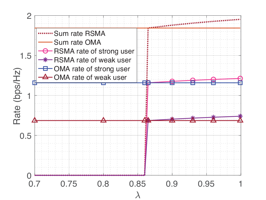
In this section, we validate the aforementioned bounds through simulation. We consider a two users scenario with interference as in [2]. Fig. 4 illustrates the variation of RSMA and OMA rates (in bps/Hz) of $s$ and $w$ w.r.t. $\lambda$. For $\gamma_{s}=6$ dB, $\gamma_{w}=2$ dB, $\beta=0$ (i.e., for perfect SIC), $P_{t}=1$ W, we have observed that with increase in $\lambda$, the $SR^{\text{rsma}}$ increases beyond $SR^{\text{oma}}$ after $\lambda=0.865$. The $\tau$ values computed using $\lambda<0.865$ are negative, which is inappropriate for computing the rates. Hence, the RSMA rates in the region, $\lambda<0.865$, are indicated as zero. The value of $\lambda=0.865$ is greater than the value derived using (24), (25), (28), and (29). This shows that the bound obtained using (24), (25), (28), and (29) is not strict. Thus, the lower bound of $\lambda$ computed using (23) and presented in Fig. 2 is validated in Fig. 4. Nevertheless, selecting the $\lambda$ using (24), (25), (28), and (29) is necessary to make the bound of $\alpha_{c}>0$. Furthermore, it is observed from Fig. 3 for $\lambda>\lambda_{\text{lower}}$ that $R^{\text{rsma}}_{s}$ and $R^{\text{rsma}}_{w}$ are greater than $R^{\text{oma}}_{s}$ and $R^{\text{oma}}_{w}$, respectively. Note that the private message of user $s$ requires more power than that of user $w$.

Fig. 5 shows the variation of rate w.r.t $\alpha_{c}$ for $\beta=0$ for the same set of $\gamma_{s}$ and $\gamma_{w}$. For $\lambda=0.99$, the lower and upper bound of $\alpha_{c}$ computed using (19) and (23), respectively, are $0.683$ and $0.776$. It is evident from the Fig. 5 that for $\alpha_{\text{LB}}<\alpha_{c}<\alpha_{\text{UB}}$, the individual RSMA rates of $s$ and $w$ are greater than their respective OMA rates. Moreover, the lower and upper bound of $\alpha_{c}$ computed using (19) and (23) are approximately equal to the $\alpha_{\text{LB}}$ and $\alpha_{\text{UB}}$ observed in Fig. 5. Furthermore, similar results are obtained by varying $\tau$ for $\lambda=0.99$ and $\alpha_{c}=0.689$. However, due to space constraints, we cannot present the plots.

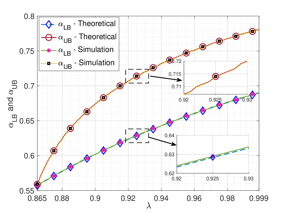
Since the derived bounds of $\tau$ as shown in (14) and (16) are functions of $\alpha_{c}$ and $\lambda$, we have plotted the variation of the bounds w.r.t $\alpha_{c}$ for $\lambda=0.99$ in Fig. 6. $\alpha_{\text{LB}}$ and $\alpha_{\text{UB}}$ are computed using (19) and (23), respectively. For $\beta=0$, $\gamma_{s}=6$ dB, and $\gamma_{w}=2$ dB, $\tau_{\text{lower}}$ and $\tau_{\text{upper}}$ are plotted by varying $\alpha_{c}$ between $\alpha_{\text{LB}}$ and $\alpha_{\text{UB}}$. We can observe that these bounds are almost equal to the theoretical bounds computed using (14) and (16). Similar results can be obtained for different $\lambda$.

Fig. 7 shows the variation of rate w.r.t. $\beta$. We can observe that as $\beta$ increases, after 0.035, the $R^{\text{rsma}}_{s}$ becomes less than $R^{\text{oma}}_{s}$. However, the $SR^{\text{rsma}}$ remains greater than $SR^{\text{oma}}$ as $\beta$ increases further. Nevertheless, after $\beta=0.05$, $SR^{\text{rsma}}$ starts deteriorating. This is due to the decrease in $\gamma_{ps}$ and $\gamma_{pw}$ with an increase in $\beta$. The result in Fig. 7 is plotted for $\lambda=0.99$, $\alpha_{c}=0.689$, and $\tau=0.1$.

In this letter, we have derived the bounds on the power allocation coefficients of the common and private messages and the fraction of the individual common message of the users for which the RSMA rates of users will be greater than their respective OMA rates. We have validated the derived bounds using simulation. We have numerically computed $\alpha_{c}$, $\lambda$, and $\tau$, which are validated using simulation. In our future work, we aim to compute the closed-form expressions of the lower bound of $\lambda$ and $\alpha_{\text{UB}}$. We also aim to derive bounds on $\beta$ in our future work.

References

- [1] Y. Mao et. al., “Rate-Splitting Multiple Access: Fundamentals, Survey, and Future Research Trends,” IEEE Commun. Surveys & Tut., vol. 24, no. 4, pp. 2073–2126, 2022.
- [2] Z. Yang et. al., “Downlink Sum-Rate Maximization for Rate Splitting Multiple access (RSMA),” in Proc. IEEE ICC, Virtual, 2020, pp. 1–6.
- [3] T. Cai et. al., “Resource Allocation for Secure Rate-Splitting Multiple Access with Adaptive Beamforming,” in Proc. IEEE ICC Workshops, Montreal, Canada, 2021, pp. 1–6.
- [4] L. Yin et. al., “Rate-Splitting Multiple Access for Multigroup Multicast Cellular and Satellite Communications: PHY Layer Design and Link-Level Simulations,” in Proc. IEEE ICC Workshops, Montreal, Canada, 2021, pp. 1–6.
- [5] B. Clerckx et. al., “Is NOMA Efficient in Multi-Antenna Networks? A Critical Look at Next Generation Multiple Access Techniques,” IEEE Open J. Commun. Soc., vol. 2, pp. 1310–1343, 2021.
- [6] W. Jaafar et. al., “Multiple Access in Aerial Networks: From Orthogonal and Non-Orthogonal to Rate-Splitting,” IEEE Open J. Veh. Technol., vol. 1, pp. 372–392, 2020.
- [7] O. Dizdar et. al., “Rate-Splitting Multiple Access to Mitigate the Curse of Mobility in (Massive) MIMO networks,” IEEE Tran. Commun., vol. 69, no. 10, pp. 6765–6780, 2021.