A Wasserstein distance-based spectral clustering method for transaction data analysis

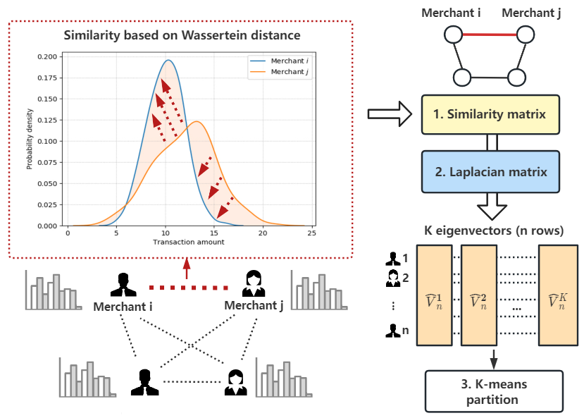
Step 1. Construct a similarity matrix based on Wasserstein distance. For $n$ merchants, let $S_{n}\in\mathbb{R}^{n\times n}$ denote the similarity matrix based on Wasserstein distance. Let function $S(\cdot,\cdot)$ denote the similarity between two distributions. Then, each element $S_{n,ij}$ is defined as $S_{n,ij}=S(i,j)=\exp\left\{-W(i,j)/\sigma\right\}$, where $W(i,j)$ is the Wasserstein distance between merchants $i$ and $j$, and $\sigma$ is the scaling hyperparameter for normalizing the Wasserstein distance function. In practice, we can set $\sigma=\sup\limits_{i,j}W(i,j)$ by default.

Step 2. Obtain the normalized Laplacian matrix. Based on the similarity matrix $S_{n}$, a normalized Laplacian matrix $L_{n}=D_{n}^{-1/2}S_{n}D_{n}^{-1/2}$ can be determined, where $D_{n}$ is a diagonal matrix with $D_{n,ii}=\sum_{j\neq i}S_{ij},1\leq i\leq n$. Because $S_{n}$ is symmetric and all elements of $S_{n}$ are non-negative, the resulting Laplacian matrix $L_{n}$ is semi-definite.

Step 3. Conduct clustering on $K$ eigenvectors of $L_{n}$. First, we obtain the $K$ largest eigenvalues of $L_{n}$ for clustering. Let $\widehat{V}_{n}^{1},\cdots,\widehat{V}_{n}^{K}$ denote the corresponding eigenvectors. We can stack the eigenvectors to form a matrix $\widehat{V}_{n}=[\widehat{V}_{n}^{1},\cdots,\widehat{V}_{n}^{K}]\in\mathbb{R}^{n\times K}$. Then, traditional clustering methods, e.g., K-means, clusters the $n$ rows of $\widehat{V}_{n}$ into $K$ clusters. Because each row of $\widehat{V}_{n}$ is related to an individual merchant, the partition of $n$ rows of $\widehat{V}_{n}$ indicates a clustering solution for all merchants. Thus, $K$ non-overlapping merchant index sets could be obtained. The clustering algorithm is summarized in Appendix E.

Remark 1. (Number of clusters) To select an appropriate value for the number of clusters in a data-driven manner, we recommend two alternative approaches. The first is the silhouette coefficient approach [49]. The second involves visualizing the eigenvalues arranged in descending order. If there is a sharp decrease between the $K^{\prime}$-th and successive eigenvalues, $K^{\prime}$ is the appropriate selection [50].

SubWSC-Step 1. Construct a normalized Laplacian matrix for the sub-graph. For convenience, we use mathcal letters to denote the notation used in the subsampling method. Let $\mathcal{L}_{n}\in\mathbb{R}^{n\times n_{s}}$ represent the normalized Laplacian matrix of the subsample, calculated as

where $\mathcal{D}_{n_{s}}$ is an $n_{s}\times n_{s}$ diagonal matrix. For the $j$-th sample, where $\phi(j)=i$, we have $\mathcal{D}_{n_{s},jj}=D_{n,ii}$.

SubWSC-Step 2. Obtain $K$ eigenvectors of $\mathcal{L}_{n}\mathcal{L}^{\top}_{n}$. Suppose that matrices $\widehat{\mathcal{U}}_{n}\in\mathbb{R}^{n\times n}$ and $\widehat{\mathcal{V}}_{n_{s}}\in\mathbb{R}^{n_{s}\times n_{s}}$ are stacked eigenvectors of $\mathcal{L}_{n}\mathcal{L}^{\top}_{n}$ and $\mathcal{L}^{\top}_{n}\mathcal{L}_{n}$, respectively. We can find the $K$ largest eigenvalues and the corresponding eigenvectors, thus generating $\widehat{\mathcal{U}}_{K}\in\mathbb{R}^{n\times K}$ and $\widehat{\mathcal{V}}_{K}\in\mathbb{R}^{n_{s}\times K}$ from $\widehat{\mathcal{U}}_{n}$ and $\widehat{\mathcal{V}}_{n_{s}}$, respectively. Specifically, we focus on $\widehat{\mathcal{U}}_{K}$ for the purpose of deducing the partition of all merchants. With limited computational resources, we can calculate $\widehat{\mathcal{U}}_{K}$ through a specific method with low computation costs, which is as follows:

where $\Sigma_{K}$ is a diagonal matrix consisting of the $K$ largest eigenvalues of $\mathcal{L}^{\top}_{n}\mathcal{L}_{n}$. Because $\widehat{\mathcal{V}}_{K}$ and $\Sigma^{-1/2}_{K}$ can be derived from the SVD of $\mathcal{L}^{\top}_{n}\mathcal{L}_{n}$, a $n_{s}\times n_{s}$ matrix, the computational complexity related to SVD in WSC can be greatly optimized.

SubWSC-Step 3. Conduct clustering on $\widehat{\mathcal{U}}_{K}$. Each row of $\widehat{\mathcal{U}}_{K}$ refers to an individual merchant. Thus, the partition of $n$ rows of $\widehat{\mathcal{U}}_{K}$ can directly lead to the partition of all merchants.

The proof of Proposition 1 is given in Appendix A.2. Proposition 1 states that given a similarity matrix, SubWSC has a much lower time cost than WSC. Thus, it can be applied to large datasets, even with limited computational resources. In real applications, to further illustrate the computational complexity of the methods and discuss the acceleration of the proposed algorithm, we make the following remarks.

Remark 2. (Total Computational Complexity of SubWSC) It is noteworthy that the similarity matrix $S_{n}$ must be computed in advance before the subsampling. The computational complexity of calculating $S_{n}$ is at least $O(n^{2})$ because it requires calculating Wasserstein distances between each pair of merchants. However, by adopting a cover tree structure [51], the calculation time can be reduced to $O(n\log n)$. See Appendix A.1 for a more detailed illustration. For the similarity matrix calculated based on the cover tree data structure, the overall computational complexity of clustering is $O(n\log n+nn_{s}^{2})$. In real applications, the selection of subsample size is a critical issue. The selection of SubWSC subsample size is discussed in the next section.

Remark 3. (Acceleration of Constructing $S_{n}$) An optional K-nearest neighbors (KNN) construction step can be considered to reconstruct the similarity matrix $S_{n}$. This is a widely applied method to improve the efficiency of spectral clustering [52]. From the graph perspective, we can drop weak relationships within the graph by this process. Let $k_{0}$ denote a threshold, e.g., $k_{0}=10$, for the neighbors of each merchant. Then, the reconstructed similarity matrix $S^{\prime}_{n}=[S^{\prime}_{n,ij}]\in\mathbb{R}^{n\times n}$ can be defined as

where $\mathcal{N}(j,k_{0})$ is the set of the $k_{0}$ nearest neighbors of merchant $i$ measured by the Wasserstein distance function. The set $\mathcal{N}(j,k_{0})$ satisfies $|\mathcal{N}(j,k_{0})|=k_{0}$, where $|\cdot|$ denotes the size of the set; $W(i,j)\leq W(i^{\prime},j)$, for any $i\in\mathcal{N}(j,k_{0})$, and $i^{\prime}\notin\mathcal{N}(j,k_{0})$.

Assumption 1 (Latent distribution): Assume that there exist $K$ underlying distributions $\{F^{*}_{1},\cdots,F^{*}_{K}\}$, such that, for each merchant $i$, $1\leq i\leq n$, the CDF $F_{i}$ is identical to one of the $K$ distributions. Let a latent variable $\gamma_{i}$ denote the relationship between merchant $i$ and the distributions. If the CDF of merchant $i$ is identical to $F^{*}_{k}$, then $\gamma_{i}=k$.

Assumption 2 (Number of transactions): Assume that $v_{\min}=\Omega(\log n)$, where $v_{\min}=\min\{v_{i}:i=1,\cdots,n\}$. The notation $g(n)=\Omega(f(n))$ indicates the existence of positive constants $c_{0}$ and $n_{0}$ such that $g(n)\geq c_{0}f(n)$ for all $n\geq n_{0}$ [53].

Assumption 3 (Similarity matrix): Assume that $d^{*}_{\min}=\Omega\left(n\right)$.

According to Assumption 1, each merchant’s CDF can match exactly one of the $K$ underlying distributions, suggesting a particular behavior pattern. Thus, $n$ merchants can be partitioned according to their behavior patterns. Let $n^{*}_{k}$ denote the number of merchants corresponding to $F^{*}_{k}$, $1\leq k\leq K$. Then, we define $n_{\max}=\max\limits_{k}n^{*}_{k}$ and $n_{\min}=\min\limits_{k}n^{*}_{k}$, which will be used in the discussions related to the clustering error rates. Assumption 2 shows that the order of $v_{\min}$ should be not less than $\log n$. For example, if a dataset contains $n=10,000$ merchants, Assumption 2 requires the minimal number of transactions per merchant to be no smaller than the order of $\log n=9.21$. This is easily satisfied in real applications. Assumption 3 requires the similarity matrix to not be too sparse, which is reasonable and easily satisfied if there are no isolated clusters or outliers. In common finite mixture models [54], it is assumed that all observations follow $\mathcal{F}^{*}=\sum_{k=1}^{K}w_{k}F^{*}_{k}$, which is a mixture of $K$ latent distributions, where $w_{k}$ is the weight for $F^{*}_{k}$ and $\sum_{k}w_{k}=1$. If we assume that the latent distributions in Assumption 1 can form a finite mixture model, it can be readily verified that $d^{*}_{\min}=\min\limits_{i}\sum_{j}E\{S(i,j)\}\geq\min\limits_{i}\sum_{j:\gamma_{j}=\gamma_{i}}E\{S(i,j)\}.$ If $i$ and $j$ have identical CDFs, we can derive that $\lim\limits_{v_{\min}\to\infty}E\{S(i,j)\}=1$ (see Appendix A.3). Because $v_{\min}=\Omega(n)$, there exist positive constants $c_{0}\leq 1$ and $n_{0}$ such that for $n\geq n_{0}$, we have $E\{S(i,j)\}\geq c_{0}$ for any $i$ and $j$ with $\gamma_{j}=\gamma_{i}$. Because $d^{*}_{\min}\geq nc_{0}\min\limits_{k}w_{k}$, we can verify that $d^{*}_{\min}=\Omega(n)$. Based on these assumptions, the proposed method is theoretically analyzed in the following subsection.

The proof of Lemma 1 is provided in Appendix B.1. According to Lemma 1, merchants $i$ and $j$ belong to the same cluster if $V_{n,i\cdot}=V_{n,j\cdot}$, namely, if their CDFs are identical. Furthermore, $V_{n}$ consists of only $K$ distinct rows, each of which is related to a single underlying distribution. K-means clustering on $V_{n}$ determines $K$ cluster centers corresponding to the $K$ underlying distributions to partition all merchants accurately. Then, we prove that the eigenvectors $\widehat{V}_{n}^{1},\cdots,\widehat{V}_{n}^{K}$ converge to those of the underlying Laplacian matrix $L^{*}_{n}$.

The proof of Theorem 1 is given in Appendix B.2. From (2), the following conclusions are derived. First, given $K$ and $\lambda_{K}$, the discrepancy between $\widehat{V}_{n}\Sigma$ and $V_{n}$ measured by Frobenius norm is $O_{p}\left(\sqrt{\log n/n}\right)$. Thus, the eigenvectors $\widehat{V}_{n}$ converge to $V_{n}$ in probability as $n\to\infty$. Because $V_{n}$ indicates the correct partition, the convergence of $\widehat{V}_{n}$ suggests that the resulting clusters converge to the correct partition of all merchants. Second, the estimation error may be reduced if $\lambda_{K}$ is relatively large, which suggests that an appropriate value has been chosen for the number of clusters.

Thus, given $\lambda_{K}$ away from 0, the clustering error rate converges to 0 in probability as $n\to\infty$. This guarantees the theoretical performance of the proposed method. The proof of Theorem 2 is given in Appendix B.4.

The proof of Theorem 3 is given in Appendix C.1. Thus, the following conclusions are drawn. First, the required subsample size is related to the number of clusters $K$. If merchants show different behavior patterns, a large $n_{s}$ is recommended. Second, if the dataset is imbalanced, where $n_{\min}/n$ could be small, a relatively large $n_{s}$ is preferred. Finally, for fixed $\alpha$ and $K$, we derive $n_{s}=\Omega(\log n)$, which is feasible for large-scale datasets. If we select $n_{s}=c\log n$, where $c$ is a constant, the computational complexity of SubWSC is $O(n\log^{2}n)$.

The proof of this theorem is given in Appendix C.4. Several conclusions can be drawn. First, it suggests that the clustering performance of SubWSC is better when $\omega_{K}$ is larger. If $K$ is fixed, then $\omega_{K}$ would be larger if the subsample led by $\mathcal{C}$ covers more merchants, especially those with different underlying CDFs. Second, given the eigenvalue $\omega_{K}$ is bounded away from 0, we obtain $\mathcal{P}_{e}=O_{p}(\log n/n)$. Thus, the resulting partition of SubWSC converges to the correct solution with $n\to\infty$ in probability. Third, the corresponding probability in Theorem 4 is relatively smaller than that in Theorem 2. Although subsampling makes the proposed method feasible for large-scale datasets, the sampling process may lead to more uncertainty during clustering. Thus, in real applications with massive data, it is helpful to find a balance between the computational efficiency and clustering performance, e.g., enlarging the subsample size when computational resources are sufficient.

Step 1. For cluster $k$, $1\leq k\leq K$, the number of within-cluster merchants is set as $n^{*}_{k}$. The total number of merchants is $n=\sum_{k=1}^{K}n^{*}_{k}$.

Step 2. For each cluster $k$, $1\leq k\leq K$, we specify a distribution $F^{*}_{k}$ as the ground truth. For any $k\neq k^{\prime}$, $F^{*}_{k}$ is different from $F^{*}_{k^{\prime}}$.

Step 3. For each merchant $i$, $1\leq i\leq n$, define $v_{i}=\max\{v_{0i},\log n\}$ as the number of transactions, where $v_{0i}$ is generated using a Poisson distribution $Poisson(\beta)$.

Step 4. For each simulated merchant $i$, $1\leq i\leq n$, let $\gamma_{i}$ denote the cluster it belongs to. Given $\gamma_{i}$, we generate $v_{i}$ transactions $(m_{i,1},\cdots,m_{i,v_{i}})$ from $F^{*}_{\gamma_{i}}$. Then, we use the absolute values $\{|m_{i,q}|\}_{q=1}^{v_{i}}$ as simulated transactions for merchant $i$.

We consider two examples by specifying the distributions $\{F^{*}_{1},\cdots,F^{*}_{K}\}$. Figure 4 shows the empirical distributions of the generated clusters with continuous and discrete distributions.

Example 1 (Continuous distributions): We set $K=3$. The ground truths $F^{*}_{1},F^{*}_{2}$, and $F^{*}_{3}$ are $N(2,2^{2})$, $Exp(\frac{1}{2})$, and $Gamma(2,1)$, respectively.

Example 2 (Discrete distributions): We again set $K=3$. First, we set three basic distributions: $F^{*}_{1}$ is set as $N(4,2^{2})$; $F^{*}_{2}$ is a mixture of $Exp(\frac{1}{2})$ and $U[10,12]$, with weights of 0.8 and 0.2, respectively; $F^{*}_{3}$ is a mixture of $Exp(\frac{1}{2})$ and $U[4,6]$, with weights 0.3 and 0.7, respectively. Then, for each merchant $i$, $1\leq i\leq n$, the transaction amount $m_{i,q}$ is replaced by the rounded value $[m_{i,q}]$, $1\leq q\leq v_{i}$, where $[\cdot]$ denotes the integer function.

Standard K-means method [33] with transaction-based features: the input features are average amount of transactions and standard deviation of transactions.

Hierarchical clustering (HC)[55] method based on the Wasserstein distance: it uses a $n\times n$ Wasserstein distance matrix with the complete-linkage agglomerative algorithm.

Kolmogorov–Smirnov K-means clustering (KSKC)[25]: this is a recently proposed method for clustering transaction data. A distance function based on the Kolmogorov–Smirnov statistic measures the dissimilarity between merchants represented using ECDF. An iterative heuristic algorithm then divides all merchants into $K$ clusters.

Comparing clustering performances. Based on Tables 1 and 2, we draw the following conclusions. First, WSC outperforms the other methods in both the continuous and discrete examples. Second, the increase in $\beta$ leads to promising improvements in the proposed method. WSC can archive better clustering performances by collecting more transaction data per merchant. Furthermore, the clustering results in Figures 5 and 6 show that K-means failed in the two examples, while WSC provided the most similar results to the ground truth.

Performance of SubWSC. Figures 7 and 8 illustrate the clustering performances and time costs of SubWSC. With increasing subsample size, the performance curves of SubWSC gradually approach those of WSC. SubWSC also achieves comparable performances with small samples. In Example 1 with $n^{*}=1,000$, when the subsample size was 30 % of the entire dataset, $\overline{\mbox{RI}}$, $\overline{\mbox{CA}}$, and $\overline{\mbox{NMI}}$ of SubWSC reached 91.7%, 90.8%, and 86.5% of those without subsampling, respectively, while the computational time was 16.2% of that for WSC. Hence, the subsampling method requires much less computational resources than WSC. Accordingly, SubWSC provides a promising solution for clustering on massive datasets when computational resources are limited.

Nesting: Once merchant $i$ appears in $CS_{l}$, then for every lower levels within the tree, there is a node associated with merchant $i$. Thus, we have $CS_{l}\subset CS_{l-1}$ for every $l$.

Covering: If merchant $g\in CS_{l-1}$, then there exists a merchant $i\in CS_{l}$ such that $S(i,g)\geq 2^{l}$. Correspondingly, node $i\textquoteright$ is a parent node of node $g\textquoteright$.

Separation: For any two nodes $i\textquoteright$ and $j\textquoteright$ within the same level $l$, the associated merchants $i,j\in CS_{l}$ satisfy $S(i,j)<2^{l}$.

WSC: According to Algorithm 1, there are two main computational costs of WSC. One is the computation of Wasserstein distance for $2^{-1}n(n-1)$ pairs of merchants. As discussed in Appendix A.1, the computational complexity of this part is at least $O(n^{2})$. The computational complexity can be improved to $O(n\log n)$ using the cover tree structure. The other is the computation of eigenvectors using SVD on $L_{n}$. The computational complexity of this step is $O(n^{3})$ because of SVD.

SubWSC: Suppose that the similarity matrix $S_{n}$ is given. According to the processes of SubWSC, the computational complexity of the most time-consuming part of WSC, i.e., SVD of the Laplacian matrix, is improved to $O(n^{3}_{s})$. Regarding the detailed processing of SubSC, we derive the following conclusions. The computational complexity of subsampling is $O(n)$, while that of eigenvector calculation, including SVD of $\mathcal{L}^{\top}_{n}\mathcal{L}_{n}$, is $O(nn^{2}_{s}+n^{3}_{s})$. Moreover, the complexity of K-means clustering on $\widehat{\mathcal{U}}_{K}$ is $O(n)$. Hence, the overall computational complexity is $O(nn^{2}_{s})$.

References

- Peppard [2000] J. Peppard, Customer relationship management (CRM) in financial services, European Management Journal 18 (2000) 312–327.
- Park and Kim [2003] C.-H. Park, Y.-G. Kim, A framework of dynamic CRM: Linking marketing with information strategy, Business Process Management Journal 9 (2003) 652–671.
- Chan [2008] C. C. H. Chan, Intelligent value-based customer segmentation method for campaign management: A case study of automobile retailer, Expert Systems with Applications 34 (2008) 2754–2762.
- Kim et al. [2010] H.-S. Kim, Y.-G. Kim, C.-W. Park, Integration of firm’s resource and capability to implement enterprise crm: A case study of a retail bank in korea, Decision Support Systems 48 (2010) 313–322.
- Khajvand and Tarokh [2011] M. Khajvand, M. J. Tarokh, Estimating customer future value of different customer segments based on adapted RFM model in retail banking context, Procedia Computer Science 3 (2011) 1327–1332.
- Wu and Chou [2011] R.-S. Wu, P.-H. Chou, Customer segmentation of multiple category data in e-commerce using a soft-clustering approach, Electronic Commerce Research and Applications 10 (2011) 331–341.
- Chiang [2012] W.-Y. Chiang, To establish online shoppers’ markets and rules for dynamic CRM systems: an empirical case study in taiwan, Internet Research 22 (2012) 613–625.
- Zhang et al. [2014] Y. Zhang, E. T. Bradlow, D. S. Small, Predicting customer value using clumpiness: From RFM to RFMC, Marketing Science 34 (2014) 195–208.
- Alborzi and Khanbabaei [2016] M. Alborzi, M. Khanbabaei, Using data mining and neural networks techniques to propose a new hybrid customer behaviour analysis and credit scoring model in banking services based on a developed RFM analysis method, International Journal of Business Information Systems 23 (2016) 1–22.
- Eisenmann and Barley [2006] T. R. Eisenmann, L. Barley, Paypal merchant services, Harvard Business School Case (2006) 806–188.
- Lowry et al. [2006] P. B. Lowry, T. M. Wells, G. D. Moody, S. Humphreys, D. Kettles, Online payment gateways used to facilitate e-commerce transactions and improve risk management, Communications of the Association for Information Systems 17 (2006) 1–48.
- Huo et al. [2011] H. Huo, Y. Wei, S. Xin, Risk analysis of the third-party payment business, in: International Conference on Management Science & Industrial Engineering, 2011, pp. 1143–1147.
- Dannenberg and Zupancic [2009] H. Dannenberg, D. Zupancic, Customer segmentation, Gabler, 2009.
- Tsiptsis and Chorianopoulos [2011] K. K. Tsiptsis, A. Chorianopoulos, Data mining techniques in CRM: Inside customer segmentation, John Wiley & Sons, 2011.
- Bult and Wansbeek [1995] J. R. Bult, T. Wansbeek, Optimal selection for direct mail, Marketing Science 14 (1995) 378–394.
- Hsu et al. [2012] F.-M. Hsu, L.-P. Lu, C.-M. Lin, Segmenting customers by transaction data with concept hierarchy, Expert Systems with Applications 39 (2012) 6221–6228.
- Khobzi et al. [2014] H. Khobzi, E. Akhondzadeh-Noughabi, B. Minaei-Bidgoli, A new application of rfm clustering for guild segmentation to mine the pattern of using banks’ e-payment services, Journal of Global Marketing 27 (2014) 178–190.
- Dhandayudam and Krishnamurthi [2013] P. Dhandayudam, I. Krishnamurthi, Customer behavior analysis using rough set approach, Journal of Theoretical and Applied Electronic Commerce Research 8 (2013) 21–33.
- Van Vlasselaer et al. [2015] V. Van Vlasselaer, C. Bravo, O. Caelen, T. Eliassi-Rad, L. Akoglu, M. Snoeck, B. Baesens, Apate: A novel approach for automated credit card transaction fraud detection using network-based extensions, Decision Support Systems 75 (2015) 38–48.
- Sakurai et al. [2008] Y. Sakurai, L. Li, R. Chong, C. Faloutsos, Efficient distribution mining and classification, in: SIAM International Conference on Data Mining, 2008, pp. 632–643.
- Kullback and Leibler [1951] S. Kullback, R. A. Leibler, On information and sufficiency, Annals of Mathematical Statistics 22 (1951) 79–86.
- Rényi et al. [1961] A. Rényi, et al., On measures of entropy and information, in: Berkeley Symposium on Mathematical Statistics and Probability, 1961, pp. 547–561.
- Lin [1991] J. Lin, Divergence measures based on the shannon entropy, IEEE Transactions on Information theory 37 (1991) 145–151.
- Vallender [1974] S. Vallender, Calculation of the wasserstein distance between probability distributions on the line, Theory of Probability & Its Applications 18 (1974) 784–786.
- Zhu et al. [2021] Y. Zhu, Q. Deng, D. Huang, B.-Y. Jing, B. Zhang, Clustering based on kolmogorov–smirnov statistic with application to bank card transaction data, Journal of The Royal Statistical Society: Series C (applied Statistics) 70 (2021) 558–578.
- Del Barrio et al. [1999] E. Del Barrio, J. A. Cuesta-Albertos, C. Matrán, J. M. Rodríguez-Rodríguez, Tests of goodness of fit based on the l2-wasserstein distance, Annals of Statistics 27 (1999) 1230–1239.
- Piccoli and Rossi [2014] B. Piccoli, F. Rossi, Generalized wasserstein distance and its application to transport equations with source, Archive for Rational Mechanics and Analysis 211 (2014) 335–358.
- Fournier and Guillin [2015] N. Fournier, A. Guillin, On the rate of convergence in wasserstein distance of the empirical measure, Probability Theory and Related Fields 162 (2015) 707–738.
- Panaretos and Zemel [2019] V. M. Panaretos, Y. Zemel, Statistical aspects of wasserstein distances, Annual Review of Statistics & Its Application 6 (2019) 405–431.
- Rüschendorf [1985] L. Rüschendorf, The wasserstein distance and approximation theorems, Probability Theory and Related Fields 70 (1985) 117–129.
- Del Barrio et al. [1999] E. Del Barrio, E. Giné, C. Matrán, Central limit theorems for the wasserstein distance between the empirical and the true distributions, Annals of Probability 27 (1999) 1009–1071.
- Piccoli and Rossi [2016] B. Piccoli, F. Rossi, On properties of the generalized wasserstein distance, Archive for Rational Mechanics and Analysis 222 (2016) 1339–1365.
- Lloyd [1982] S. Lloyd, Least squares quantization in PCM, IEEE Transactions on Information Theory 28 (1982) 129–137.
- Hagen and Kahng [2002] L. Hagen, A. B. Kahng, New spectral methods for ratio cut partitioning and clustering, IEEE Transactions on Computer-Aided Design of Integrated Circuits and Systems 11 (2002) 1074–1085.
- Chung and Graham [1997] F. R. Chung, F. C. Graham, Spectral graph theory, American Mathematical Soc., 1997.
- Nascimento and De Carvalho [2011] M. C. Nascimento, A. C. De Carvalho, Spectral methods for graph clustering–a survey, European Journal of Operational Research 211 (2011) 221–231.
- Kannan et al. [2004] R. Kannan, S. Vempala, A. Vetta, On clusterings: Good, bad and spectral, Journal of the ACM 51 (2004) 497–515.
- Von Luxburg et al. [2008] U. Von Luxburg, M. Belkin, O. Bousquet, Consistency of spectral clustering, Annals of Statistics 36 (2008) 555–586.
- Song et al. [2008] Y. Song, W.-Y. Chen, H. Bai, C.-J. Lin, E. Y. Chang, Parallel spectral clustering, in: Joint European Conference on Machine Learning and Knowledge Discovery in Databases, 2008, pp. 374–389.
- Chen and Cai [2011] X. Chen, D. Cai, Large scale spectral clustering with landmark-based representation, in: AAAI Conference on Artificial Intelligence, 2011, pp. 313–318.
- Law et al. [2017] M. T. Law, R. Urtasun, R. S. Zemel, Deep spectral clustering learning, in: International Conference on Machine Learning, 2017, pp. 1985–1994.
- Halko et al. [2011] N. Halko, P.-G. Martinsson, J. A. Tropp, Finding structure with randomness: Probabilistic algorithms for constructing approximate matrix decompositions, SIAM Review 53 (2011) 217–288.
- Menon and Elkan [2011] A. K. Menon, C. Elkan, Fast algorithms for approximating the singular value decomposition, ACM Transactions on Knowledge Discovery from Data 5 (2011) 1–36.
- Dhillon et al. [2013] P. Dhillon, Y. Lu, D. P. Foster, L. Ungar, New subsampling algorithms for fast least squares regression, in: Advances in Neural Information Processing Systems, 2013, pp. 360–368.
- Wang et al. [2018] H. Wang, R. Zhu, P. Ma, Optimal subsampling for large sample logistic regression, Journal of the American Statistical Association 113 (2018) 829–844.
- Ai et al. [2021] M. Ai, F. Wang, J. Yu, H. Zhang, Optimal subsampling for large-scale quantile regression, Journal of Complexity 62 (2021) 101512.
- Politis et al. [1999] D. N. Politis, J. P. Romano, M. Wolf, Subsampling, Springer Science & Business Media, 1999.
- Delattre et al. [2004] S. Delattre, S. Graf, H. Luschgy, G. Pages, Quantization of probability distributions under norm-based distortion measures, Statistics & Decisions 22 (2004) 261–282.
- Rousseeuw [1987] P. J. Rousseeuw, Silhouettes: A graphical aid to the interpretation and validation of cluster analysis, Journal of Computational and Applied Mathematics 20 (1987) 53–65.
- Filippone et al. [2008] M. Filippone, F. Camastra, F. Masulli, S. Rovetta, A survey of kernel and spectral methods for clustering, Pattern Recognition 41 (2008) 176–190.
- Beygelzimer et al. [2006] A. Beygelzimer, S. Kakade, J. Langford, Cover trees for nearest neighbor, in: International Conference on Machine Learning, 2006, p. 97–104.
- Aksoylar et al. [2017] C. Aksoylar, J. Qian, V. Saligrama, Clustering and community detection with imbalanced clusters, IEEE Transactions on Signal and Information Processing over Networks 3 (2017) 61–76.
- Knuth [1976] D. E. Knuth, Big omicron and big omega and big theta, ACM Sigact News 8 (1976) 18–24.
- Shedden [2015] B. M. Shedden, Finite mixture modeling with mixture outcomes using the em algorithm, Biometrics 55 (2015) 463–469.
- Defays [1977] D. Defays, An efficient algorithm for a complete link method, The Computer Journal 20 (1977) 364–366.
- Fahad et al. [2014] A. Fahad, N. Alshatri, Z. Tari, A. Alamri, I. Khalil, A. Y. Zomaya, S. Foufou, A. Bouras, A survey of clustering algorithms for big data: Taxonomy and empirical analysis, IEEE Transactions on Emerging Topics in Computing 2 (2014) 267–279.
- Geršgorin [1931] S. Geršgorin, über die abgrenzung der eigenwerte einer matrix, Bulletin de l’Académie des Sciences de l’URSS. Classe des sciences mathématiques et na 6 (1931) 749–754.
- Tropp [2012] J. A. Tropp, User-friendly tail bounds for sums of random matrices, Foundations of Computational Mathematics 12 (2012) 389–434.
- Bobkov and Ledoux [2019] S. Bobkov, M. Ledoux, One-dimensional empirical measures, order statistics, and kantorovich transport distances, Memoirs of the American Mathematical Society 261 (2019) 1–80.
- Chung et al. [2006] F. Chung, F. R. Chung, F. C. Graham, L. Lu, K. F. Chung, et al., Complex graphs and networks, 107, American Mathematical Soc., 2006.
- Yu et al. [2015] Y. Yu, T. Wang, R. J. Samworth, A useful variant of the davis–kahan theorem for statisticians, Biometrika 102 (2015) 315–323.
- Mackey et al. [2014] L. Mackey, M. I. Jordan, R. Y. Chen, B. Farrell, J. A. Tropp, Matrix concentration inequalities via the method of exchangeable pairs, Annals of Probability 42 (2014) 906–945.