Null Cosmic Strings: Scattering by Black Holes, Optics and Spacetime Content

A trajectory of a null string in a space-time $\cal M$ with coordinates $x^{\mu}$ is defined as $x^{\mu}=x^{\mu}(\lambda,\tau)$, where $\lambda$ and $\tau$ are real parameters. The trajectory is fixed by equations [1]:

$$(l\cdot l)=0~~,~~~(\eta\cdot\eta)>0~~~,$$

(2.1)

$$(l\cdot\eta)=0~~,$$

(2.2)

$$\nabla_{l}l=\beta l~~.$$

(2.3)

where $l^{\mu}\equiv x^{\mu}_{~,\lambda}$ and $\eta^{\mu}\equiv x^{\mu}_{~,\tau}$ are the tangent vectors, notation $(u\cdot v)$ stands for the scalar product of vectors $u$, $v$ in the tangent space of $\cal M$. $\lambda$ is an affine parameter if $\beta=0$. We assume that velocity of the string $l$ is future-directed. $\eta$ is called the connecting vector.

Since any point of the string moves as a light ray, trajectories of null strings can be considered as a one-dimensional analogue of null geodesic congruences (NGC). Though one cannot create a one-dimensional string-like congruence of light rays, the cross-section of such NGC cannot be constant as a result of expansion or contraction in the gravitational field.

To define the string scalars $\theta$, $\kappa$ one sets at each point of the string trajectory a tetrade $l,n,p,q$. Here $p=\eta/|\eta|$, $|\eta|^{2}=(\eta\cdot\eta)$, $n$ is null, orthogonal to $p$ and normalized as $(n\cdot l)=-2$, vector $q$ is spacelike, unit, and orthogonal to $l,n,p$. Condition $|\eta|\neq 0$ is assumed.

The parameters $\theta$ and $\kappa$ are introduced as the following spin coefficients [7] :

$$\theta=(p\cdot\nabla_{p}l)~~~,~~~\kappa=(q\cdot\nabla_{p}l)~~.$$

(2.4)

(Relation to notations of [7] is $\theta=\theta_{s}$, $\kappa=\kappa_{2}$). Spin coefficients (2.4) are invariant with respect to null rotations of the tetrade:

$$l^{\prime}=l~~,~~p^{\prime}=p~~,~~n=n^{\prime}+2\omega q^{\prime}+\omega^{2}l^{\prime}~~,~~q=q^{\prime}+\omega l^{\prime}~~~.$$

(2.5)

Rotations (2.5) and reparametrizations of $\lambda,\tau$,

$$\lambda^{\prime}=g(\lambda,\tau)~~,~~\tau^{\prime}=\phi(\tau)~~,$$

(2.6)

make a 2-parameter group of $l$-preserving null rotations of $n,p,q$, accompanied with rescalings of $l$ and $n$, see [7]. Parameters $\theta$ and $\kappa$ transform as boost-weighted scalars, $Q=(g_{,\lambda})^{b}Q^{\prime}$, with boost weight $b=1$.

We also use a pair of null complex vectors:

$$m={1\over\sqrt{2}}(p+iq)~~,~~\bar{m}={1\over\sqrt{2}}(p-iq)~~.$$

(2.7)

Invariants in optical equation (1.1) are

$$\Psi_{0}=-C_{mlml}~~,~~\Phi_{00}=-\frac{1}{2}R_{ll}~~,$$

(2.8)

where $C_{abcd}$ and $R_{ab}$ are components, respectively, of the Weyl tensor Ricci tensor in the given basis, see [12], [13]. Definitions (2.8) are introduced on the string trajectory.

We start with the case of a straight string in Minkowsky spacetime. If the string is parallel to the $z$-axis and moves along the $x$-axis its stress-energy tensor is

$$T^{\mu\nu}(x)=\mu\delta(y)\delta(u)l^{\mu}l^{\nu}~~,$$

(2.9)

where $u=t-x$, $l^{\mu}\partial_{\mu}=\partial_{t}+\partial_{x}$. The parameter $\mu$ is the energy of the string per unit length. Stress-tensor (2.9) was found in [2] by applying the Aichelburg-Sexl boost [11] to the stress-energy tensor of a straight massive (tensile) cosmic string. The same boost applied to the Riemann tensor results in a non-trivial component $R_{uyuy}=\omega\delta(y)\delta(u)$, where $\omega=8\pi G\mu$. The null string leaves the spacetime locally flat but creates a non-trivial holonomy at the string worldsheet: a parallel transport of a vector around a point of the string trajectory results in a null rotation defined by (2.5) with $\omega=8\pi G\mu$.

As it is easy to see, definition (2.9) implies a standard covariant conservation law

$$\nabla_{\mu}T^{\mu\nu}(x)=0~~,$$

(2.10)

for a constant parameter $\mu$, or, in general, if

$$\left.\partial_{l}\mu\right|_{u=y=0}=0~~.$$

(2.11)

The last condition allows $\mu$ to vary along the string, $\mu=\mu(z)$. Such a string creates a locally flat spacetime with a non-constant holonomy, where $\omega=\omega(z)=8\pi G\mu(z)$.

Consider now a null string in an arbitrary spacetime $\cal M$ with the trajectory $x^{\mu}=\bar{x}^{\mu}(\lambda,\tau)$. A natural generalization of (2.9) is the following stress-energy tensor of the string:

$$T^{\mu\nu}(x)=\int d\lambda d\tau~\bar{\mu}(\lambda,\tau)~\delta^{4}(x,\bar{x})~l^{\mu}(\bar{x})l^{\nu}(\bar{x})~~,$$

(2.12)

where $\bar{\mu}(\lambda,\tau)$ is some density, $\delta^{4}(x,\bar{x})=\delta^{4}(x-\bar{x})/\sqrt{-g}$ is an invariant delta-function with the support on the string trajectory, $l^{\mu}(\bar{x})=d\bar{x}^{\mu}/d\lambda$. Note that $\bar{\mu}(\lambda,\tau)$ transforms as

$$\bar{\mu}(\lambda,\tau)=\phi_{,\tau}g^{-1}_{,\lambda}~\bar{\mu}^{\prime}(\lambda^{\prime},\tau^{\prime})~~$$

(2.13)

under reparametrizations (2.6). After some algebra one can check that covariant conservation law (2.10) holds for SET (2.12) under the condition:

$$\partial_{\lambda}\bar{\mu}+\beta\bar{\mu}=0~~,$$

(2.14)

where $\beta$ is defined in (2.3). In what follows we assume that $\lambda$ is affine parameter. In this case $\bar{\mu}$ does not depend on $\lambda$.

It is instructive to see how definition (2.12) reduces to (2.9) in case of straight string in Minkowsky spacetime. String trajectory is given by equations: $t=\lambda$, $x=\lambda$, $z=\tau$, $y=0$. Integration over $\lambda$ in (2.12) yields $\delta(u)$, integration over $\tau$ results in (2.9) with $\mu=\bar{\mu}(z)$.

One expects a null string creates a local holonomy around each point $x^{\mu}=\bar{x}^{\mu}(\lambda,\tau)$ with a parameter $\omega=\omega(\lambda,\tau)$. By using example of a straight string in Minkowsky spacetime, the physical energy of the string $\mu=\mu(\lambda,\tau)$ can be introduced as a parameter which determines the local holonomy by relation $\omega(\lambda,\tau)=8\pi G\mu(\lambda,\tau)$. To understand connection between $\bar{\mu}$ and $\mu$ we need to bring SET (2.12), at a chosen point $x^{\mu}_{\ast}=\bar{x}^{\mu}(\lambda_{\ast},\tau_{\ast})$, to “flat form” (2.9). This can be done in local coordinates, where $g_{\mu\nu}(x_{\ast})=\eta_{\mu\nu}$, $\Gamma^{\rho}_{\mu\nu}(x_{\ast})=0$, $x_{\ast}=0$, and string equations (2.1)-(2.3) have a simple solution near $x_{\ast}$,

$$t\simeq\lambda-\lambda_{\ast}~~,~~x\simeq\lambda-\lambda_{\ast}~~,~~y=0~~,~~z\simeq z_{,\tau}(\tau_{\ast})(\tau-\tau_{\ast})~~.$$

(2.15)

Then $T^{\mu\nu}(x)$ near $x_{\ast}$ takes form (2.9) with the physical energy

$$\mu(\lambda,\tau)=\bar{\mu}(\tau)|\eta(\lambda,\tau)|^{-1}~~,$$

(2.16)

where factor $|\eta(\lambda,\tau)|=|z_{,\tau}(\tau_{\ast})|$ appears when integrating over $\tau$. The key difference between $\mu$ and $\bar{\mu}$ is that $\mu$ does not depend on reparametrizations of $\tau$, see (2.6). Stress-energy tensor (2.12) in terms of the physical energy looks as

$$T^{\mu\nu}(x)=\int d\lambda~|\eta|d\tau~\mu~\delta^{4}(x,\bar{x})~l^{\mu}(\bar{x})l^{\nu}(\bar{x})~~.$$

(2.17)

Element $|\eta|d\tau$ is the physical length of a segment of the string between $\bar{x}^{\mu}(\lambda,\tau)$ and $\bar{x}^{\mu}(\lambda,\tau+d\tau)$.

Energy conservation law (1.2) follows from (2.16) and definition (2.4) of $\theta$.

Since the string energy $\mu(\lambda,\tau)$ is determined with respect to the physical length of a string segment, it develops singularities at points where connecting vector $\eta$ has vanishing norm, $\eta^{2}=0$. These may be isolated points or a one-parameter family $\lambda=\lambda_{c}(\tau)$ on the string trajectory which makes a curve

$$x^{\mu}_{c}(\tau)\equiv x^{\mu}(\lambda_{c}(\tau),\tau)~~.$$

(2.18)

Condition $\eta^{2}=0$ implies that either $\eta=0$ or $\eta$ is a null vector at $\lambda=\lambda_{c}(\tau)$. If $\eta=0$, the tangent vector $\zeta$ to curve (2.18) is $\zeta=\dot{x}_{c}=\dot{\lambda}_{c}~l$. That is, $\zeta$ is null and directed along $l$. If $\eta$ becomes null at $\lambda=\lambda_{c}(\tau)$, it follows from (2.2) that $\eta$ should be directed along $l$. Then $\zeta=\dot{\lambda}_{c}~l+\eta$ is null and it is again directed along $l$. Therefore, curve (2.18) is a light-like caustic where trajectories of different points of the string are tangent to.

Optical equation (1.1) implies the following behavior of the string scalar and string energy near a caustic:

$$Z(\lambda,\tau)\sim{1\over\lambda-\lambda_{c}(\tau)}~~,$$

(2.19)

$$\mu(\lambda,\tau)\sim{\mu_{c}(\tau)\over|\lambda-\lambda_{c}(\tau)|}~~,$$

(2.20)

where $\mu_{c}(\tau)$ is some function.

Caustics of null strings, like caustics in optics, are the regions where energy is concentrated. For this reason caustics are distinctive properties of null strings which may result in important physical effects.

By using SET (2.12) one can define conserved charges $Q$ of the null string. If a spacetime admits a Killing vector field $\zeta$,

$$Q(\zeta)=\int_{\Sigma}d\Sigma_{\mu}~J^{\mu}(\zeta)~~,~~J^{\mu}(\zeta)=T^{\mu\nu}\zeta_{\nu}~~.$$

(2.21)

Integration in (2.21) goes over a Cauchy hypersurface $\Sigma$.

We consider null strings in asymptotically flat spacetimes and use (2.21) to define “in” and “out” linear and angular momenta of the string at past null infinity $\mathcal{I}^{-}$ and future null infinity $\mathcal{I}^{+}$. Points of null strings near $\mathcal{I}^{\pm}$ move as almost radial light rays. The metric near $\mathcal{I}^{-}$, $\lambda\to-\infty$, can be written as

$$ds^{2}\simeq-dv^{2}+2dvdr+r^{2}d\Omega^{2}~~.$$

(2.22)

The string trajectory is $r_{\mathrm{in}}\simeq|\lambda|$, $v_{\mathrm{in}}=0$, $\theta_{\mathrm{in}}=\theta_{\mathrm{in}}(\tau)$, $\varphi_{\mathrm{in}}=\varphi_{\mathrm{in}}(\tau)$. Near $\mathcal{I}^{+}$, $\lambda\to\infty$,

$$ds^{2}\simeq-du^{2}-2dudr+r^{2}d\Omega^{2}~~,$$

(2.23)

$r_{\mathrm{out}}\simeq\lambda$, $u_{\mathrm{out}}=0$, $\theta_{\mathrm{out}}=\theta_{\mathrm{out}}(\tau)$, $\varphi_{\mathrm{out}}=\varphi_{\mathrm{out}}(\tau)$. The corresponding conserved charges near $\mathcal{I}^{-}$ and $\mathcal{I}^{+}$, respectively, are

$$Q_{\mathrm{in}}(\zeta)=\int_{r=R}\sqrt{-g}J_{\mathrm{in}}^{r}(\zeta)dv~d\theta d\varphi~~,~~Q_{\mathrm{out}}(\zeta)=\int_{r=R}\sqrt{-g}J_{\mathrm{out}}^{r}(\zeta)du~d\theta d\varphi~~.$$

(2.24)

Surfaces $\Sigma_{\mathrm{in}}$ and $\Sigma_{\mathrm{out}}$ in (2.24) are taken at $r=R$. One finds with the help of (2.12), (2.21)

$$Q_{\mathrm{in}}(\zeta)=\int d\tau\bar{\mu}(\tau)(l_{\mathrm{in}}\cdot\zeta)~~,~~Q_{\mathrm{out}}(\zeta)=\int d\tau\bar{\mu}(\tau)(l_{\mathrm{out}}\cdot\zeta)~~.$$

(2.25)

The integration in (2.24) over $u,v,\theta,\varphi$ is performed by using equations of radial trajectories.

To give preliminary definitions we begin with null strings in Minkowsky spacetime. If $\lambda$ is an affine parameter, general solution to (2.1) – (2.3) is

$$x^{\mu}(\lambda,\tau)=\lambda b^{\mu}(\tau)+a^{\mu}(\tau)~~,$$

(3.1)

where $b^{\mu}$ is an arbitrary null vector, $b^{2}=0$. Restrictions on $a^{\mu}$ are: $(b\cdot\dot{a})=0$, see (2.2), and $\dot{a}^{2}>0$, $\dot{a}\equiv a_{,\tau}$. One finds:

$$|\eta|^{2}=\lambda^{2}\dot{b}^{2}+2\lambda(\dot{b}\cdot\dot{a})+\dot{a}^{2}~~.$$

(3.2)

A residual freedom, $\lambda\to\lambda+g(\tau)$, can be fixed by additional physical conditions, for example, $(l\cdot u_{o})=-1$, $(\eta\cdot u_{o})=0$, where $u_{o}$ is the 4-velocity of observers, see [7]. In Minkowsky coordinates, where velocity of observers is $u_{o}^{\mu}=\delta^{\mu}_{0}$, these conditions are ensured if $t(\lambda,\tau)=\lambda$, that is $\dot{a}$ and $\dot{b}$ have only spatial components. Let $|\dot{b}|\neq 0$, then [7]

$$Z(\lambda,\tau)={1\over\lambda+z_{0}(\tau)}~~,~~z_{0}(\tau)=r(\tau)e^{i\varphi(\tau)}~~.$$

(3.3)

$$\cos\varphi\equiv{(\dot{b}\cdot\dot{a})\over|\dot{a}||\dot{b}|}~~,~~r\equiv{|\dot{a}|\over|\dot{b}|}~~,$$

(3.4)

$Z(\lambda,\tau)$ is a solution to (1.1) with $\Psi_{0}=\Phi_{00}=0$.

It is easy to see from (3.2) that caustics of null strings discussed in Sec.2.3 appear when $\dot{a}(\tau)=-\lambda_{c}(\tau)\dot{b}(\tau)$, $\eta=0$. In this case $Z(\lambda,\tau)=1/(\lambda-\lambda_{c}(\tau))$, in agreement with (2.19).

One can represent $Z(\lambda,\tau)$ in another form. For example, if $\bar{\theta}(\tau)$ and $\bar{\kappa}(\tau)$ are expansion and rotation of the string, say, at $\lambda=0$, then

$$Z(\lambda,\tau)={\bar{\theta}(\tau)+i\bar{\kappa}(\tau)\over\lambda(\bar{\theta}(\tau)+i\bar{\kappa}(\tau))+1}$$

(3.5)

Caustics in (3.5) appear when $\bar{\kappa}(\tau)=0$, $\lambda=\lambda_{c}(\tau)=-1/\bar{\theta}(\tau)$.

As for $\bar{\theta}(\tau)$ and $\bar{\kappa}(\tau)$, these parameters can be expressed in terms of more convenient characteristics of a “snapshot” of the string at $\lambda=0$. One can use the Frenet frame,

$$\vec{E}_{1}=\frac{\dot{\vec{a}}}{|\dot{\vec{a}}|}~~,~~\dot{\vec{E}}_{1}=k_{1}\vec{E}_{2}~~,~~\dot{\vec{E}}_{2}=-k_{1}\vec{E}_{1}+k_{2}\vec{E}_{3}~~,~~\dot{\vec{E}}_{3}=-k_{2}\vec{E}_{2}$$

(3.6)

to define curvature $k_{1}(\tau)$ and torsion $k_{2}(\tau)$ of curve $\vec{x}(0,\tau)=\vec{a}(\tau)$. Vector $\vec{b}$ can be chosen as

$$\vec{b}(\tau)=\cos\alpha(\tau)~\vec{E}_{2}+\sin\alpha(\tau)~\vec{E}_{3}~~.$$

(3.7)

It can be shown that

$$\bar{\theta}=-\frac{k_{1}\cos\alpha}{|\dot{\vec{a}}|}~~,~~\bar{\kappa}=\frac{\dot{\alpha}+k_{2}}{|\dot{\vec{a}}|}$$

(3.8)

Thus, the curvature of $\vec{x}(0,\tau)$ determines expansion of the string, while its rotation depends on the torsion of $\vec{x}(0,\tau)$.

There is a particular class of strings with $\dot{b}\equiv 0$. For such a class $Z\equiv 0$. From (3.5) one concludes that in this case $\bar{\theta}(\tau)=\bar{\kappa}(\tau)=0$, and $\dot{\alpha}=0$, see (3.7). Equations (3.8) imply that $k_{2}=0$, and $k_{1}=0$ or $\cos\alpha=0$. This means that the string is a straight line, or the curve $\vec{x}(0,\tau)=\vec{a}(\tau)$ lies in a plane, and $\vec{b}$ is orthogonal to the plane, $(b\cdot\dot{a})=(b\cdot\ddot{a})=0$.

We call strings with $Z\equiv 0$ frozen strings, since they preserve their form during the evolution. A simple example of the frozen string is a straight string.

The aim of this Section is to study scattering of a null string by a black hole, or a gravitating source, in general. Analysis of string equations (2.1) - (2.3) for null strings near massive sources can be quite complicated [14]-[19]. We do calculations in the weak field approximation for strings which move far from the sources, that is, with large impact parameters. Our aim is to understand some universal features of the string dynamics. Analogous scattering problems for tensile strings have been studied in [8],[9],[10]. Scattering on non-rotating black holes can be found in [20]

Suppose a black hole is located at the center of coordinates $x=y=z=0$. The mass of the black hole and its angular momentum are, respectively, $M$, $J^{i}$. In the weak-field approximation the flat metric

$$ds^{2}=-dt^{2}+dx^{2}+dy^{2}+dz^{2}~~$$

(3.9)

acquires corrections

$$\delta g_{\mu\nu}=h^{M}_{\mu\nu}+h^{J}_{\mu\nu}~~$$

(3.10)

with the following non-zero components:

$$h^{M}_{00}=\frac{r_{g}}{r}~~,~~h^{M}_{ij}=\frac{r_{g}\,x_{i}x_{j}}{r^{3}}~~,$$

(3.11)

$$h^{J}_{0i}=2G~\varepsilon_{ijk}\frac{x^{j}J^{k}}{r^{3}}~~,$$

(3.12)

where $r_{g}=2MG$, $r=\sqrt{x^{2}+y^{2}+z^{2}}$. We denote coordinates of the string trajectory at $\mathcal{I}^{-}$ by $x_{\mathrm{in}}$,

$$x(\lambda,\tau)_{\lambda\to-\infty}\to x_{\mathrm{in}}(\lambda,\tau)=\lambda b_{\mathrm{in}}(\tau)+a_{\mathrm{in}}(\tau)~~,$$

(3.13)

and by $x_{\mathrm{out}}$ at $\mathcal{I}^{+}$, after the scattering on the source,

$$x(\lambda,\tau)_{\lambda\to\infty}\to x_{\mathrm{out}}(\lambda,\tau)=\lambda b_{\mathrm{out}}(\tau)+a_{\mathrm{out}}(\tau)~~.$$

(3.14)

Velocities of the string are $l_{\mathrm{in}}=b_{\mathrm{in}}$, at $\mathcal{I}^{-}$, and $l_{\mathrm{out}}=b_{\mathrm{out}}$, at $\mathcal{I}^{+}$.

For further use it is convenient to introduce a minimal distance $r_{0}(\tau)$ between the center of coordinates and a segment of the string with parameter $\tau$. In the absence of the source, $r^{2}=\lambda^{2}+2\lambda(b_{\mathrm{in}}\cdot a_{\mathrm{in}})+a_{\mathrm{in}}^{2}$ has a minimum at $\lambda=\lambda_{0}=-(b_{\mathrm{in}}\cdot a_{\mathrm{in}})$. One can define

$$\vec{x}_{0}(\tau)=\vec{x}_{\mathrm{in}}(\lambda_{0},\tau)=\vec{a}_{\mathrm{in}}-\vec{b}_{\mathrm{in}}(b_{\mathrm{in}}\cdot a_{\mathrm{in}})~~,~~r_{0}(\tau)=|\vec{x}_{0}(\tau)|=\sqrt{a^{2}_{\mathrm{in}}-(b_{\mathrm{in}}\cdot a_{\mathrm{in}})^{2}}~~.$$

(3.15)

We are looking for effects of metric perturbations (3.11), (3.12) in the linear approximation in $M$ and $J$, $x=x_{\mathrm{in}}+\delta_{M}x+\delta_{J}x$, when change of the string trajectory is determined by linearized version of (2.3) (with $\beta=0$)

$$\partial_{\lambda}^{2}~\delta x^{\mu}+\delta\Gamma^{\mu}_{\alpha\beta}(x_{\mathrm{in}})~l_{\mathrm{in}}^{\alpha}l_{\mathrm{in}}^{\beta}=0~~.$$

(3.16)

Here $\delta\Gamma^{\mu}_{\alpha\beta}(x_{\mathrm{in}})$ are calculated on $x_{\mathrm{in}}$ with the help of (3.11), (3.12). This is the scattering with large impact parameter, $r_{0}(\tau)\gg r_{g}$.

In this Section we assume that the black hole is non-rotating, $J^{i}=0$. At large $r$ the effects of the non-zero angular momentum are weaker than effects caused by the mass. They are considered in Sec. 3.3.

It is clear that solutions to (3.16) differ by additions of the form $\lambda c^{\mu}(\tau)+d^{\mu}(\tau)$, where $c^{\mu}(\tau)$ and $d^{\mu}(\tau)$ are arbitrary 4-vectors. The solution is uniquely fixed by requiring conditions (2.1), (2.2), and $l^{2}=0$. We also require that $(l\cdot u_{o})\to-1$, $(\eta\cdot u_{o})\to 0$ at $\mathcal{I}^{+}$, where $u_{o}^{\mu}=\delta^{\mu}_{0}$ is 4-velocity of the chosen set of observers.

The solution to (3.15) which satisfies these conditions in the linear approximation in $r_{g}$ is

$$t(\lambda,\tau)=\lambda-r_{g}~\ln\left[{r_{\mathrm{in}}-\lambda-(a_{\mathrm{in}}\cdot b_{\mathrm{in}})\over\varrho}\right]~~,$$

(3.17)

$$\vec{x}(\lambda,\tau)=\vec{x}_{\mathrm{in}}(\lambda,\tau)-r_{g}~{\vec{x}_{0}(\tau)\over r_{\mathrm{in}}-\lambda-(a_{\mathrm{in}}\cdot b_{\mathrm{in}})}~~,$$

(3.18)

where $\varrho$ is some dimensional parameter.

We need scattering data at $\mathcal{I}^{+}$, where (3.17), (3.18) become

$$t(\lambda,\tau)\simeq\lambda-r_{g}~\ln{r_{0}^{2}\over\lambda\varrho}~~,$$

(3.19)

$$\vec{x}(\lambda,\tau)\simeq\lambda\vec{b}_{\mathrm{out}}+\vec{a}_{\mathrm{out}}=\vec{x}_{\mathrm{out}}(\lambda,\tau)~~,$$

(3.20)

$$\vec{b}_{\mathrm{out}}=\vec{b}_{\mathrm{in}}-\Phi~\vec{n}~~,~~~~\Phi={2r_{g}\over r_{0}}~~,$$

(3.21)

$$\vec{a}_{\mathrm{out}}=\vec{a}_{\mathrm{in}}-\Phi~(a_{\mathrm{in}}\cdot b_{\mathrm{in}})~\vec{n}~~,~~\vec{n}={\vec{x}_{0}\over r_{0}}~~,$$

(3.22)

One can check that $|\vec{b}_{\mathrm{out}}|=1$ up to terms $O(\Phi^{2})$. Thus, scattering results in rotation of the string velocity $l_{\mathrm{in}}=b_{\mathrm{in}}$ in the plane $b_{\mathrm{in}},a_{\mathrm{in}}$ by angle $\Phi$,

$$l^{i}_{\mathrm{out}}=M_{ij}~l^{j}_{\mathrm{in}}~~,$$

(3.23)

$$M_{ij}\simeq\delta_{ij}+\Phi~\omega_{ij}~~,~~\omega_{ij}=r_{0}^{-1}(b_{\mathrm{in}}^{i}a_{\mathrm{in}}^{j}-b_{\mathrm{in}}^{j}a_{\mathrm{in}}^{i})~~.$$

(3.24)

This effect is similar to deflection of light rays by massive bodies in general relativity.

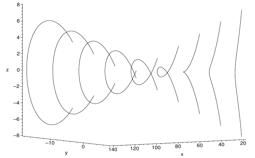
It should be pointed out that even in the weak field approximation evolution of a null string described by (3.17), (3.18) may be non-trivial due to creation of loops and caustics. The simplest illustration how null strings form loops is the scattering of a straight string. The world-sheet of the string is shown on Figure 1. The string equation at $\mathcal{I}^{-}$ is taken as $t=x=\lambda$, $z=\tau$, $y=\rho$, where $\rho$ is an impact parameter. The black hole is located at the center of coordinates. The results are obtained for the ratio $2MG/\rho=0.1$. Figure 2 demonstrates scattering of a finite segment of the same string and creation of a caustic at an isolated point. Figure 3 depicts the norm $|\eta|$ of the connecting vector. The caustic appears when $|\eta|=0$.

It is instructive to compare these results with scattering of tensile cosmic strings [8], [9], [10], [20]. Astrophysical tensile cosmic strings are expected to move with the velocity $v\simeq 0,7c$. At such velocities straight tensile strings, as a result of scattering by a black hole, are displaced in the direction perpendicular to their motion [20]. At velocities $0,9c<v<1c$ scattering of ultrarelativistic tensile cosmic strings reveals formation of loops which is similar to the case of null strings [20]. As has been pointed out in [10], in the ultrarelativistic limit of a string moving very near the speed of light in a direction perpendicular to the string, the propagation of disturbances along the string suffers a large time dilation, so that each piece of the string is effectively decoupled and moves very nearly along a null geodesic.

As a next step, we use Sec. 2.4 to analyze how energy, linear momentum and angular momentum of the string are changed during the scattering. The energy corresponds to the Killing vector $\zeta=\partial_{t}$ and it conserves,

$$E_{\mathrm{in}}=\int d\tau\bar{\mu}(\tau)=E_{\mathrm{out}}~~.$$

(3.25)

For linear momenta ($\zeta=\partial_{i}$) one has

$$\vec{P}_{\mathrm{in}}=\int d\tau\bar{\mu}(\tau)\vec{l}_{\mathrm{in}}~~,~~\vec{P}_{\mathrm{out}}=\int d\tau\bar{\mu}(\tau)\vec{l}_{\mathrm{out}}~~.$$

(3.26)

$$\vec{P}_{\mathrm{out}}=\vec{P}_{\mathrm{in}}-\int d\tau\bar{\mu}(\tau)\Phi(\tau)~\vec{n}(\tau)~~.$$

(3.27)

Consider an axis which goes through the center of coordinates and is directed along a unit vector $\vec{Z}$. The angular momentum $j(Z)$ of the string related to rotations around the given axis is a charge for the Killing field $\zeta^{i}=-\varepsilon_{ijk}x^{j}Z^{k}$. The angular momentum at $\mathcal{I}^{-}$ is

$$j_{\mathrm{in}}(Z)=-\int d\tau\bar{\mu}(\tau)(\vec{l}_{\mathrm{in}}\cdot[\vec{x}_{\mathrm{in}}\times\vec{Z}])=-\int d\tau\bar{\mu}(\tau)(\vec{l}_{\mathrm{in}}\cdot[\vec{a}_{\mathrm{in}}\times\vec{Z}])~~.$$

(3.28)

Change of the angular momentum at $\mathcal{I}^{+}$ depends on variations of $l_{\mathrm{in}}$ and $a_{\mathrm{in}}$,

$$\delta j(Z)=-\int d\tau\bar{\mu}(\tau)\left((\delta\vec{l}\cdot[\vec{a}_{\mathrm{in}}\times\vec{Z}])+(\vec{l}_{\mathrm{in}}\cdot[\delta\vec{a}\times\vec{Z}])\right)~~.$$

(3.29)

However, if (3.21) and (3.22) are used in (3.29), the variation vanishes,

$$\delta j(Z)=-\int d\tau\bar{\mu}(\tau)~\Phi~(\vec{x}_{0}\cdot[\vec{n}\times\vec{Z}])=0~~.$$

(3.30)

The string does not change its angular momentum.

By the conservation laws the black hole after interaction with the string receives a non-zero linear momentum

$$\vec{P}_{\mathrm{body}}=\vec{P}_{\mathrm{in}}-\vec{P}_{\mathrm{out}}=\int d\tau\bar{\mu}(\tau)\Phi(\tau)~\vec{n}(\tau)~~,$$

(3.31)

see (3.27).This is the gravitational recoil effect.

To give an example of the recoil effect consider again the scattering of the straight string. Suppose that string energy $\mu$ is constant. Calculation of the recoil momentum yields the only non-zero component, along $y$ axis,

$$P^{y}_{\mathrm{body}}=2\pi r_{g}\mu~~.$$

(3.32)

The corresponding change of the energy of the body, $\delta E\sim MG^{2}\mu^{2}$, can be neglected in the linear approximation. The momentum may be different if string energy depends on $z$. For example, another component of the momentum, $P^{z}_{\mathrm{body}}$, may be non-trivial.

We focus now on physical effects related to angular momenta of black holes. Scattering of tensile cosmic strings on rotating black holes can be found in [21]-[23]. Angular momentum transfer from rotating black holes to tensile strings may result in interesting effects. For example, a tensile cosmic string piercing a rotating black hole may spin-down the black hole [24] such that the angular momentum vector of the black hole aligns with the string [25].

To proceed we put $h_{\mu\nu}^{M}=0$ in (3.10). The solution to (3.16) with the same choice of asymptotic conditions which lead to (3.17), (3.18) is the following:

$$t(\lambda,\tau)=\lambda-{2G~r_{0}\over r_{\mathrm{in}}(r_{\mathrm{in}}-\lambda-(a_{\mathrm{in}}\cdot b_{\mathrm{in}}))}(J\cdot c)~~,$$

(3.33)

$$\vec{x}(\lambda,\tau)=\vec{x}_{\mathrm{in}}(\lambda,\tau)+2G~\frac{2(J\cdot c)~[\vec{b}_{\mathrm{in}}\times\vec{c}]+[\vec{J}\times\vec{d}]}{r_{\mathrm{in}}-\lambda-(a_{\mathrm{in}}\cdot b_{\mathrm{in}})}-2G~\frac{(J\cdot c)}{r_{0}}(\vec{d}+\vec{b}_{\mathrm{in}})~~,$$

(3.34)

where

$$\vec{c}=\frac{[\vec{a}_{\mathrm{in}}\times\vec{b}_{\mathrm{in}}]}{r_{0}}~~,~~\vec{d}=\frac{\lambda~\vec{b}_{\mathrm{in}}+\vec{a}_{\mathrm{in}}}{r_{\mathrm{in}}}~~.$$

(3.35)

With the help of (3.33), (3.34) one finds that the angular momentum results in rotation of initial vectors $a_{\mathrm{in}}$, $b_{\mathrm{in}}$ which determine trajectory of the string at $\mathcal{I}^{-}$,

$$b^{i}_{\mathrm{out}}=b^{i}_{\mathrm{in}}+\frac{4G}{r_{0}^{2}}\varepsilon_{ijk}~b^{j}_{\mathrm{in}}\left(2(J\cdot c)~c^{k}-J^{k}\right)~~,$$

(3.36)

$$a^{i}_{\mathrm{out}}=a^{i}_{\mathrm{in}}+\frac{4G(J\cdot b_{\mathrm{in}})}{r_{0}^{2}}\varepsilon_{ijk}~a^{j}_{\mathrm{in}}b^{k}_{\mathrm{in}}+\frac{4G(J\cdot c)}{r_{0}^{2}}\left(2(a_{\mathrm{in}}\cdot b_{\mathrm{in}})n^{i}-r_{0}~b^{i}_{\mathrm{in}}\right)~~.$$

(3.37)

Variation of the angular momentum of the string can be computed with the help of (2.25), (3.36), (3.37),

$$\delta j(Z)=4G\int d\tau\frac{\bar{\mu}}{r_{0}^{2}}(Z\cdot[\vec{J}\times[\vec{a_{\mathrm{in}}}\times\vec{b_{\mathrm{in}}}]])~~.$$

(3.38)

Equation (3.38) can be interpreted as a spin-spin interaction. Variation of the angular momentum due to the mass of the source vanishes, see (3.29), (3.30), while the spin-spin interaction is a non-trivial effect.

The simplest example is a straight string considered in Sec. 3.2. In this case $(a_{\mathrm{in}}\cdot b_{\mathrm{in}})=0$, and variation (3.38) can be written as

$$\delta\vec{j}=-4\pi\mu G[\vec{J}\times\vec{p}]\,\mathrm{sign}(a_{\mathrm{in}}^{y})~~,$$

(3.39)

where $p^{i}=\delta^{i}_{z}$ is the unit vector along the string (directed along the $z$-axis).

If the conservation of the total angular momentum is taken into account one comes to the following variation of the angular momentum of the black hole:

$$\delta\vec{J}=4\pi\mu G[\vec{J}\times\vec{p}]\,\mathrm{sign}(a_{\mathrm{in}}^{y})~~.$$

(3.40)

The momentum rotates around the string axis, the rotation angle being determined by the string energy only. The sign of rotation in (3.40) depends on the position of the black hole with respect to the world-sheet of the string. If the string moves between two rotating black holes it causes a non-trivial relative rotation of their angular momenta by the angle $8\pi\mu G$.

Results of Secs. 3.2, 3.3 can be interpreted as change of the velocity and angular momentum of a black hole in the gravitational field of a null string. Transformations of trajectories of massive particles and light rays in the gravitational field of the string have been studied in [2], [3] by using holonomy of spacetime created by a null string. It is instructive to see that Secs. 3.2, 3.3 reproduce results of [2] for the case of a straight null string. Transformation of a vector $V^{\mu}$ under a parallel transport around the string is

$$(V^{\prime})^{0}=\left(1+{\omega^{2}\over 2}\right)V^{0}-{\omega^{2}\over 2}V^{x}+\omega V^{y}~~,$$

(3.41)

$$(V^{\prime})^{x}=\left(1-{\omega^{2}\over 2}\right)V^{x}+{\omega^{2}\over 2}V^{0}+\omega V^{y}~~,$$

(3.42)

$$(V^{\prime})^{y}=V^{y}+\omega(V^{0}-V^{x})~~,~~(V^{\prime})^{z}=V^{z}~~,$$

(3.43)

where $\omega=8\pi\mu G$. As before, the string is assumed to be directed along the $z$ axis and move in the $x$ direction. Eqs. (3.41)–(3.43) are null transformations which are reduced to (2.5) in the case of the tetrade $l,n,p,q$.

If the string moves between two massive bodies which are initially at rest, (3.41)–(3.43) imply that the bodies acquire a relative coordinate velocity toward each other, in the direction orthogonal to the string,

$$v^{y}\simeq\omega=8\pi\mu G~~$$

(3.44)

(in the limit when $\omega\ll 1$). This result is in agreement with (3.32) which yields coordinate velocity of each body $|v^{y}_{\mathrm{body}}|\simeq 4\pi\mu G$.

According to (3.41)–(3.43), in the linear in $\omega$ approximation, a parallel transport of a spin 4-vector with components $J^{0}=0,J^{i}$, generates the rotation

$$\delta\vec{J}=\omega[\vec{J}\times\vec{p}]~~.$$

(3.45)

The parameter $\omega$ is the angle of relative rotation of two spins when the string moves between them. Equation (3.45) coincides with (3.40).

Therefore “holonomy variations” of velocities and spins of test bodies caused by gravitational field of a null cosmic string are in complete agreement with their “scattering variations”. Note that the scattering data are Noether charges (2.21) defined by the stress-energy tensor of null strings. The above analysis yields a check of introduced SET (2.12). The check is non-trivial since “scattering variations” (3.32), (3.40) are determined by independent contributions from all segments of the string.

One can also use solution (3.21), (3.22) to see how expansion and rotation parameters of the string at $\mathcal{I}^{-}$ and $\mathcal{I}^{+}$ are related. For simplicity we assume that the strings are “unfrozen” at $\mathcal{I}^{-}$. For such strings the asymptotics of optical scalars at $\mathcal{I}^{-}$ and $\mathcal{I}^{+}$ are, respectively,

$$Z_{\mathrm{in}}(\lambda,\tau)=\frac{1}{\lambda}+\frac{z_{\mathrm{in}}}{\lambda^{2}}+O(\lambda^{-3})~~,$$

(3.46)

$$Z_{\mathrm{out}}(\lambda,\tau)=\frac{1}{\lambda}+\frac{z_{\mathrm{out}}}{\lambda^{2}}+O(\lambda^{-3})~~.$$

(3.47)

Expansion is $\theta=1/\lambda+\Re~z/\lambda^{2}+...$, the rotation is $\kappa=\Im~z/\lambda+...$. After some algebra one gets

$$\Re~z_{\mathrm{out}}=\Re~z_{\mathrm{in}}+\frac{2r_{g}}{r_{0}^{4}}\left[r_{0}^{4}\ln\frac{\varrho}{r_{0}}+r_{0}^{2}\left((\dot{a}_{\mathrm{in}}\cdot\dot{a}_{\mathrm{in}})-(a_{\mathrm{in}}\cdot b_{\mathrm{in}})^{2}\right)\right.$$

$$\left.+(\dot{b}_{\mathrm{in}}\cdot a_{\mathrm{in}})^{2}\left((a_{\mathrm{in}}\cdot b_{\mathrm{in}})^{2}+a_{\mathrm{in}}^{2}\right)-2(\dot{a}_{\mathrm{in}}\cdot a_{\mathrm{in}})^{2}\right],$$

(3.48)

$$(\Im~z_{\mathrm{out}})^{2}=(\Im~z_{\mathrm{in}})^{2}-\frac{4r_{g}}{r_{0}^{4}}\left[r_{0}^{2}\left((\dot{a}_{\mathrm{in}}\cdot a_{\mathrm{in}})(a_{\mathrm{in}}\cdot b_{\mathrm{in}})+(\dot{a}_{\mathrm{in}}\cdot\dot{a}_{\mathrm{in}})\Re~z_{\mathrm{in}}\right)+\right.$$

$$\left.(\dot{b}_{\mathrm{in}}\cdot a_{\mathrm{in}})\left((\dot{a}_{\mathrm{in}}\cdot a_{\mathrm{in}})+(\dot{b}_{\mathrm{in}}\cdot a_{\mathrm{in}})^{2}\Re~z_{\mathrm{in}}\right)\left(a_{\mathrm{in}}^{2}+(a_{\mathrm{in}}\cdot b_{\mathrm{in}})^{2}\right)-2(\dot{a}_{\mathrm{in}}\cdot a_{\mathrm{in}})^{2}\left((a_{\mathrm{in}}\cdot b_{\mathrm{in}})+\Re~z_{\mathrm{in}}\right)\right]~~,$$

(3.49)

where $r_{0}=r_{0}(\tau)$.

References

- [1] A. Schild, Classical Null Strings, Phys. Rev. D16 (1977) 1722.
- [2] D.V. Fursaev, Physical effects of massless cosmic strings, Phys. Rev. D96 (2017) no.10, 104005, e-Print: arXiv:1707.02438 [gr-qc].
- [3] D.V. Fursaev, Massless Cosmic Strings in Expanding Universe, Phys. Rev. D98 (2018) no.12, 123531, e-Print: arXiv:1811.01563 [gr-qc].
- [4] T.W.B. Kibble, Topology of Cosmic Domains and Strings, J. Phys. A9 (1976) 1387-1398.
- [5] A. Vilenkin, E.P. S. Shellard, Cosmic Strings and Other Topological Defects, Cambridge University Press, 2000.
- [6] T. M. Adamo, E. T. Newman, C. N. Kozameh, Null Geodesic Congruences, Asymptotically Flat Space-Times and Their Physical Interpretation, Living Rev. Rel. 12 (2009) 6, Living Rev. Rel. 15 (2012) 1, e-Print: arXiv: 0906.2155 [gr-qc].
- [7] D.V. Fursaev, Optical equations for null strings, Phys. Rev. D103 (2021) no.12, 123526, e-Print: arXiv:2104.04982 [gr-qc].
- [8] S. Lonsdale and I. Moss, The Motion of Cosmic Strings Under Gravity, Nucl. Phys. 298 (1988) 693.
- [9] V.P. Frolov and J. De Villiers, Scattering of straight cosmic strings by black holes: Weak field approximation, Phys. Rev. D58 (1998) 105018, e-Print: arXiv:9804087 [gr-qc].
- [10] D. Page, Gravitational capture and scattering of straight test strings with large impact parameters, Phys. Rev. D58 (1998) 105026, e-Print: arXiv:9804088 [gr-qc].
- [11] C. Barrabes, P.A. Hogan, W. Israel, The Aichelburg-Sexl boost of domain walls and cosmic strings, Phys.Rev. D66 (2002) 025032, e-Print: gr-qc/0206021.
- [12] R. Penrose and W. Rindler, Spinors and Space-time. Vol. 2: Spinor and Twistor Methods in Space-time Geometry, Cambridge University Press, 1988.
- [13] S. Chandrasekhar, The mathematical theory of black holes, Oxford, UK: Clarendon (1992) 646 p.
- [14] S. Kar, Schild’s null strings in flat and curved backgrounds, Phys. Rev. D53 (1996) 6842-6846, e-Print: hep-th/9511103 [hep-th].
- [15] C.O. Lousto, N.G. Sanchez, String dynamics in cosmological and black hole backgrounds: The Null string expansion, Phys. Rev. D54 (1996) 6399-6407, e-Print: gr-qc/9605015 [gr-qc].
- [16] M.P. Dabrowski, A.L. Larsen, Null strings in Schwarzschild space-time, Phys. Rev. D55 (1997) 6409-6414, e-Print: hep-th/9610243 [hep-th].
- [17] P.I. Porfyriadis, D. Papadopoulos, Null strings in Kerr space-time, Phys. Lett. B417 (1998) 27-32, e-Print: hep-th/9707183 [hep-th].
- [18] M.P. Dabrowski, A.L. Larsen, Strings in homogeneous background space-times, Phys. Rev. D57 (1998) 5108-5117, e-Print: hep-th/9706020 [hep-th].
- [19] M.P. Dabrowski, I. Prochnicka, Null string evolution in black hole and cosmological spacetimes, Phys. Rev. D66 (2002) 043508, e-Print: arXiv: hep-th/0201180.
- [20] J. P. De Villiers and V. P. Frolov, Gravitational scattering of cosmic strings by nonrotating black holes, Class. Quant. Grav. 16 (1999) 2403-2425, e-Print: arXiv:gr-qc/9812016 [gr-qc].
- [21] M. Snajdr, V. P. Frolov and J. P. DeVilliers, Scattering of a long cosmic string by a rotating black hole, Class. Quant. Grav. 19 (2002) 5987-6008, e-Print: arXiv:gr-qc/0208009 [gr-qc].
- [22] M. Snajdr and V. P. Frolov, Capture and critical scattering of a long cosmic string by a rotating black hole, Class. Quant. Grav. 20 (2003) 1303-1320, e-Print: arXiv:gr-qc/0211018 [gr-qc].
- [23] F. Dubath, M. Sakellariadou and C. M. Viallet, Scattering of cosmic strings by black holes: Loop formation, Int. J. Mod. Phys. D16 (2007) 1311-1325, e-Print: arXiv:gr-qc/0609089 [gr-qc].
- [24] V.P. Frolov and J.Boos, Stationary black holes with stringy hair, Phys. Rev. D97 (2018) no.2, 024024, e-Print: arXiv:1711.06357 [gr-qc].
- [25] H. Xing, Yu. Levin, A. Gruzinov, and A. Vilenkin, Spinning black holes as cosmic string factories, Phys. Rev. D103 (2021) no.8, 083019, e-Print: arXiv:2011.00654 [gr-qc].
- [26] T. Madler and J. Winicour, Bondi-Sachs Formalism, Scholarpedia 11 (2016) 33528, e-Print: arXiv:1609.01731 [gr-qc].
- [27] D. J. Gross and P. F. Mende, The High-Energy Behavior of String Scattering Amplitudes, Phys. Lett. B197 (1987) 129.
- [28] D. J. Gross and P. F. Mende, String Theory Beyond the Planck Scale, Nucl. Phys. B303 (1988) 407.
- [29] Seung-Joo Lee, W. Lerche, T. Weigand, Emergent Strings from Infinite Distance Limits, JHEP 02 (2022), 190, e-Print: 1910.01135 [hep-th].
- [30] F. Xu, On TCS manifolds and 4D emergent strings, JHEP 10 (2020) 045, e-Print: 2006.02350 [hep-th].
- [31] S. Sarangi, S.H.H. Tye, Cosmic string production towards the end of brane inflation, Phys. Lett. B536 (2002) 185-192, e-Print: hep-th/0204074 [hep-th].
- [32] E.J. Copeland, R.C. Myers, J. Polchinski, Cosmic F and D strings, JHEP 06 (2004) 013, e-Print: hep-th/0312067 [hep-th].
- [33] A.L. Larsen, Chaotic string capture by black hole, Class. Quant. Grav. 11 (1994) 1201-1210, e-Print: arXiv:hep-th/9309086.
- [34] A.V. Frolov, A.L. Larsen, Chaotic scattering and capture of strings by black hole, Class. Quant. Grav. 16 (1999) 3717-3724, e-Print: arXiv:gr-qc/9908039.
- [35] T. Damour and A. Vilenkin, Gravitational wave bursts from cosmic strings, Phys. Rev. Lett. 85 (2000) 3761, e-Print: arXiv:0004075 [gr-qc].
- [36] The LIGO Scientific Collaboration, the Virgo Collaboration, the KAGRA Collaboration: R. Abbott, and others, Constraints on Cosmic Strings Using Data from the Third Advanced LIGO-Virgo Observing Run, Phys. Rev. Lett. 126 (2021) no.24, 241102, e-Print: arXiv:2101.12248 [gr-qc].