Online Adversarial Stabilization of
Unknown Networked SystemsJournal: POMACSVolume: 71263DOI: 10.1145/3579452Journal: JACMVolume: 3741118Journal: POMACSVolume: 71263DOI: 10.1145/3579452CCS: Theory of computation Adversary modelsCCS: Theory of computation Distributed algorithmsCCS: Theory of computation Online learning algorithmsCCS: Theory of computation Quadratic programming
Abstract.
We investigate the problem of stabilizing an unknown networked linear system under communication constraints and adversarial disturbances. We propose the first provably stabilizing algorithm for the problem. The algorithm uses a distributed version of nested convex body chasing to maintain a consistent estimate of the network dynamics and applies system level synthesis to determine a distributed controller based on this estimated model. Our approach avoids the need for system identification and accommodates a broad class of communication delay while being fully distributed and scaling favorably with the number of subsystems.
Keywords:
online control; learning-based control; adversarial control; distributed control; stability; communication delay1. Introduction
Large-scale networked dynamical systems play a crucial role in many emerging engineering systems such as the power grid (Fang et al. 2011), autonomous vehicles (Li et al. 2015), and swarm robots (Morgan et al. 2014). Motivated by the success of learning-based control methods for single-agent (centralized) linear systems, there has been growing interest in learning distributed controllers for unknown networked systems composed of interconnected and spatially distributed linear time-invariant (LTI) subsystems (Bu et al. 2019; Fattahi et al. 2020; Furieri et al. 2020; Ye et al. 2021; Li et al. 2021b).
However, since most existing literature ports centralized learning-based control techniques over to the distributed setting, almost all previous work assumes that the underlying dynamics are stable, or that a stabilizing and distributed controller is known. For a large-scale networked system, such assumptions are often unrealistic, because designing stabilizing distributed controllers itself is a significant task even if the dynamics model is available (Rotkowitz and Lall 2005; Han and Skelton 2003; Wang et al. 2014; Fardad and Jovanović 2014; Anderson et al. 2019; Zheng et al. 2020).
Recent work has begun to lift the assumption of the knowledge of a stabilizing controller in the centralized case, e.g. (Chen and Hazan 2021; Hu et al. 2022; Simchowitz et al. 2018). This line of work follows the approach of system identification, either by letting the unstable system run open-loop or by exciting the system via control inputs. However, such approaches induce explosive transient behaviors due to the instability of the underlying system. Without proper generalization to the networked setting, such explosive behavior can cause catastrophic system degradation before a proper stabilizing controller can be learned.
Further, until now, scalability and information constraints have only been considered separately in learning-based distributed controller design; no general approach exists. On the other hand, information constraints and scalability have been the central topics in distributed control for the past decade due to their theoretical challenge and practical importance (Rotkowitz 2008; Zheng et al. 2017; Sturz et al. 2020; Matni and Chandrasekaran 2016; Wang et al. 2018; Sturz et al. 2020). Therefore, it is crucial to simultaneously consider such constraints when designing learning-based distributed control algorithms for networked systems.
1.1. Contributions
In this work, we overcome the aforementioned challenges by leveraging recent advances in online learning and distributed control. In particular, we propose an approach that combines a distributed version of nested convex body chasing (NCBC), in order to maintain a consistent estimate of the network dynamics, with system level synthesis (SLS), in order to determine a distributed controller based on the selected consistent model. This combination yields the first online algorithm that provably stabilizes a networked LTI system with information constraints under adversarial disturbances (Theorem 4.5). The proposed algorithm (Algorithm ) is distributed and scales favorably to the number of subsystems in the network.
The proposed approach in this paper is fundamentally different than traditional system identification based methods, which incur prohibitively large state norm under adversarial disturbances, even in the simplest setting (see Table 1). The reason is that system identification-based approaches seek to learn the full system dynamics, which requires full excitation of the system against worst-case disturbances. On the other hand, our approach does not require precise knowledge of the system. Instead, we maintain model estimates that are consistent with the observations generated by the unknown system at all times. A consequence of focusing on consistency is a natural endogenous exploration-exploitation scheme where our algorithm performs well (small state norm) while the selected model stays consistent, and gains information about the system whenever it observes a large state norm that renders the selected model inconsistent.
The main result of this paper is an input-to-state stability guarantee (Theorem 4.5), where we draw novel connections between the path length property of NCBC techniques and system stability analysis. This follows from a set of novel technical results for SLS in the learning-based control context. In particular, we generalize a previous result (Anderson et al. 2019) on the characterization of the closed loop under SLS controllers that are synthesized from an arbitrary and potentially incorrect system model (Lemma 3.2). This result enables the analysis of our algorithm when each subsystem uses local, asynchronous, and wrong model information for local controller synthesis. Further, we derive a novel perturbation result with explicit constants for finite-horizon SLS synthesis (Theorem 3.4) that globally bounds the sensitivity of the optimal solution to the SLS problem (a quadratic program with equality and sparsity constraints) with respect to the model. This result is also applicable in other contexts such as a class of MPC problems studied in (Borrelli et al. 2017; Alonso et al. 2021; Sieber et al. 2021).
| Algorithm | Correlated Gaussian (Top ) | Uniform (Top ) | State-dependent (Top ) |
|---|---|---|---|
| This work | () | () | () |
| SysID | () | () | () |
1.2. Related work
This work contributes to a large and growing body of work on the topics related to learning-based control design, online control, and distributed control. We briefly review the literature most related to this work below.
Stabilization of unknown systems. Stabilizing unknown linear systems has long been a fundamental problem studied in adaptive control theory (Ioannou and Fidan 2006). It recently reemerged as a learning problem and received considerable attention from the machine learning community (Perdomo et al. 2021; Zhao et al. 2021; Treven et al. 2021; Hu et al. 2022). Most works have been developed under single-agent setting, with a no-noise assumption (Lamperski 2020; Talebi et al. 2021b) or Gausssian noise models (Faradonbeh et al. 2018; Lale et al. 2022). Under the adversarial noise setting, which is the focus of this paper, the only work that guarantees stabilization for LTI systems is (Chen and Hazan 2021), with a system identification-based approach that achieves order-optimal regret. In contrast, we propose a novel framework for stabilization under adversarial noise that does not rely on accurate identification of the true dynamics. In particular, our method is the first algorithm to stabilize a networked LTI system under adversarial disturbances with information constraints while simultaneously achieving magnitudes of improvement in empirical performance over the state-of-the-art identification-based approach (Chen and Hazan 2021) in the single-agent setting, despite the regret-optimal guarantee in (Chen and Hazan 2021).
Distributed control. Motivated by large-scale cyberphysical systems that are composed of physically distributed subsystems with local dynamical interactions, there is a large body of work on control design for networked systems (Zheng et al. 2020; Anderson et al. 2019; Kashyap and Lessard 2019). Cyberphysical systems such as the power grid are commonly constrained by a communication layer that allows specific structure of information exchange among the subsystems. such information structure imposes significant challenges for optimal control design, often rendering the problem NP-hard (Tsitsiklis and Athans 1985). In (Rotkowitz and Lall 2005), it was shown that a large class of practically relevant distributed control problems is convex and tractable to solve. Since then, many works have focused on this class of problems (Lamperski and Lessard 2015; Fardad and Jovanović 2014). However, (Wang et al. 2019) observes that the complexity of computation and implementation of distributed controllers developed under this setting can be prohibitively expensive, thus not scalable to large-scale systems. The System Level Synthesis (SLS) framework is developed as a scalable alternative to distributed control design (Anderson et al. 2019). In particular, SLS allows order-constant complexity for synthesis and implementation, due to its special parameterization and implementation of the feedback controller. As a result, many works have adopted SLS as the basis for novel (learning-based) control algorithms in both distributed and centralized setting (Dean et al. 2020a; Didier et al. 2022; Alonso et al. 2021; Umenberger and Schön 2020). We contribute to the literature on SLS by developing a suit of technical results for SLS controllers that can find applications beyond the setting of this work.
Learning distributed controllers. Many learning-based control algorithms for networked systems adopt a centralized learning or computational approach with the objective of regret minimization, e.g., (Fattahi et al. 2020; Bu et al. 2019; Ye et al. 2021; Faradonbeh and Modi 2022; Furieri et al. 2020). All prior work use the stochastic noise or no-noise model and assume a known stabilizing distributed controller is given (Li et al. 2021b; Alonso et al. 2021; Jing et al. 2021; Alemzadeh and Mesbahi 2019; Talebi et al. 2021a; Alemzadeh et al. 2021). As far as we are aware, no previous work accommodates communication delay while doing both learning and control. The most related to our work are (Ho and Doyle 2019) and (Fattahi et al. 2020), where learning-based SLS controllers are designed to control unknown networked systems. Both of the methods require the knowledge of a stabilizing and distributed controller. (Ho and Doyle 2019) is only applicable to small-uncertainty scenarios, while (Fattahi et al. 2020) requires a stabilizing distributed controller and performs centralized learning. In this work, we focus on stabilization and propose the first distributed learning-based control algorithm that guarantees stability for unknown networked systems under adversarial disturbances.
Online learning. The problem of online stabilization for unknown dynamical systems is an instance of online decision making problems, where an agent makes a sequence of decisions based on the feedback from an unknown environment with the goal of cost minimization. Online decision making is studied extensively in the online learning literature, with a line of work (Goel and Wierman 2019; Shi et al. 2020; Yeh et al. 2022; Lin et al. 2022) that makes interesting connections between convex function and body chasing (Antoniadis et al. 2016; Argue 2022) and linear control theory. In particular, (Ho et al. 2021) proposes an online nonlinear robust control method based on convex body chasing that guarantees finite mistakes under adversarial disturbances without the need for system identification. While (Ho et al. 2021) considers binary cost functions, we present novel technical results that establish the first connection between convex body chasing and stability analysis for both single-agent and networked linear dynamical systems.
1.3. Notation
Let be the norm and be the Frobenius norm. We denote the th position of a matrix as and use for the th column and th row of respectively. We use for the set of positive integers up to . Positive integers are denoted as . Bold face lower cases are reserved for vector signal of the form with is an infinite sequence of vectors indexed by time . We reserve bold face capital letters for causal linear operators/transfer matrices with components such that
We write to mean that . Given any binary matrix , we say for a matrix if the sparsity of is . We use for the standard basis in .
2. Preliminaries and problem setup
We consider the task of stabilizing an unknown networked system made up of interconnected, heterogeneous linear time-invariant (LTI) subsystems, illustrated in Figure 1(a). For each subsystem , let , , be the local state, control, and disturbance vectors respectively. Each subsystem has dynamics,
| (1) |
where we write if the states or control actions of subsystem affect those of subsystem through the open-loop network dynamics (). Concatenating all the subsystem dynamics, we can represent the global dynamics as
| (2) |
where , , , with and , and we define for all . The networked LTI model (1) has been extensively studied in the networked control literature for various applications such as robotic swarms (Mukherjee and Vu 2022), voltage control for the distribution network of the power grid (Yeh et al. 2022), and many other large-scale cyber-physical systems (Lemos and Pinto 2012; Zhang and Zhou 2016). An example is the linearized swing equation for power systems, where the global system is composed of a mesh of interacting buses (Gholami and Sun 2020; Wang and Matni 2016). In this setting, the states of each bus is two-dimensional and corresponds to the phase angle relative to some given setpoint and the associated frequency. The input at bus is the controllable load, while is the bounded load disturbances that are often correlated in space and time.
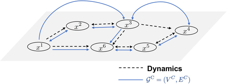
We assume that the topology among the subsystems is known, i.e., the sets for are known. However, the parameters of the dynamics (entries of matrices , ) are unknown. Let denote the unknown local parameter for subsystem , i.e., . Further, let be the global parameter. We write and (equivalently , ) to emphasize that and are matrices constructed with appropriate zeros according to the network topology (known), and the nonzero entries specified by (unknown).
Example 0.
Consider the networked system in Figure 1(a) where each subsystem has and . For each , the set contains the subsystems that has a dashed arrow pointing towards in the figure. For example, . Each and for is a scalar. The stacked global dynamics has matrix and with structure shown in Figure 1(b). The unknown local parameter corresponds to the entries of the row of and , while the global parameter is a vector containing entries in matrix and .
We now introduce three core assumptions needed for our algorithm and analysis. As we highlight below, these are standard assumptions in the learning-based control literature.
Assumption 1 (Adversarial disturbances).
for (2).
Assumption 2 (Compact Parameter Set).
The network structure for is known. The true system parameter is an element of a known compact convex set , which is a product space of local parameter sets where . The known parameter set is bounded such that there exists a known constant where for all .
Assumption 3 (Controllability).
For all , is controllable.
Bounded adversarial disturbances is a common model in the adversarial online learning and control problems (Agarwal et al. 2019; Hazan et al. 2020; Didier et al. 2022). Since we make no assumptions on how large the bound on the disturbance is, Assumption 1 models a variety of disturbance models, such as bounded and correlated stochastic noise or state-dependent disturbances such as the linearization and discretization error for nonlinear continuous dynamics (Tu 2019). Moreover, the known bound can be relaxed to an unknown parameter with for a known constant to reduce conservatism for large . Assumptions 2 and 3 are standard in the learning-based control literature, e.g., see (Cohen et al. 2019; Agarwal et al. 2019). We impose controllability in Assumption 3 for ease of exposition but it can be relaxed to stabilizability by adjusting the choice of model-based controller to an infinite-horizon controller such as the one proposed in (Yu et al. 2021) for the algorithm.
2.1. Stability
One of the fundamental goals for control design is to ensure stability. In this paper, we aim to learn a stabilizing controller for the networked linear system (2) in the sense of input to state stability (ISS) (Sontag 2008). ISS is one of the main notions of stability for both linear and nonlinear systems (Jiang and Wang 2001; Aswani et al. 2013). Here we adapt the ISS definition to the -norm.
Definition 2.2 (ISS).
A dynamical system of the form (2) is said to be input to state stable (ISS) if there exist functions that is continuous, strictly increasing, and bijective with respect to the second argument with for all , , and that is continuous, strictly increasing, and bijective such that for all initial state , disturbance sequence , and time for , we have .
2.2. Distributed design and information constraints
For large-scale networks such as the power grid with state dimension in the orders of thousands to millions, it is unrealistic and prohibitively costly for a central agent to learn a global policy online. A promising remedy is to decompose the global policy learning into a local one, where each subsystem in the network learns a local policy in a distributed fashion. In this work, we propose a distributed learning-based control algorithm for the networked linear system (2) that guarantees stability of the global system.
In addition to distributed design, networks of the form (1) are often modelled with additional information constraints that require careful consideration. In this work we consider two common information constraints. The first is communication delay, where the dynamical system is endowed with a communication network that specify delayed information transmission among subsystems. The second is local information, where each subsystem only computes with (delayed) local information within a specified neighborhood, and discard information outside of the neighborhood. We come back to these information constraints and present definitions in Sections 4.1 and 4.2.
2.3. Algorithm preliminaries
Our proposed algorithm makes use of two emerging techniques, one from the learning community, i.e., nested convex body chasing (NCBC), and one from the control community, i.e., system level synthesis (SLS). We provide important background on each below before introducing our algorithm in the next section.
2.3.1. Preliminaries on NCBC
The Nested Convex Body Chasing (NCBC) problem is a well-studied online learning problem (Bubeck et al. 2020; Argue et al. 2021). At every round , the player is presented a convex body which is nested in the previous body, e.g., . The player selects a point with the objective of minimizing the total path length of the selection for rounds, e.g., . There are many algorithms for the NCBC problem such as greedy projection of the previously selected point onto the current body (Argue et al. 2019). Among these, the Steiner point selector has been shown to achieve optimal competitive ratio against the offline optimal selector (Bubeck et al. 2020). The Steiner point of a convex body can be interpreted as the average of the extreme points and is defined as
where and the expectation is taken with respect to the uniform distribution over the unit ball. The Steiner point selector achieves the following total path length,
| (3) |
We note that the Steiner point can be approximated with any accuracy by solving sampling based linear programs, (Argue et al. 2021, Algorithm 3).
2.3.2. Preliminaries on SLS
Even when the dynamics (1) is known, it remains challenging to design distributed and localized control policies that accommodates communication delay and information constraints due to nonconvexity and computational scalability issues. Motivated by this problem, (Wang et al. 2019) introduces the SLS framework that synthesizes distributed controllers by parameterizing controllers with the closed-loop system responses induced under them. In (Dean et al. 2019; Dean et al. 2020b; Fattahi et al. 2020), SLS plays a central role for model-based learning algorithm design and analysis.
We illustrate SLS via a simple example. Consider a fixed static controller such that . Then the system (2) has the following closed-loop responses to the exogenous disturbances ,
| (4) |
where we absorb the initial state into . Instead of directly synthesizing , SLS optimizes the linear operators that map to and . Let and . Then (4) can be written as and . In signal and transfer matrix form, and . We call and with components and the closed-loop responses. More generally, for a fixed linear causal controller , the closed loop dynamics of (2) can be written in signal/transfer matrix notation as
| (5) |
where is the block-downshift operator with identity matrices of size by in all the first block sub-diagonal positions and zeros everywhere else. Operator are block diagonal matrices with matrix and on the diagonal respectively. We can similarly derive the closed-loop responses and from (5) as
Therefore, SLS uses the closed-loop responses and as the alternative parameterization for controller . The following theorem characterizes an affine subspace of the achievable system responses and under some feedback linear controller .
Theorem 2.3 (Adapted from (Anderson et al. 2019)).
For system (2), any linear causal operators with finite impulse response of horizon and satisfying the following
| (6a) | ||||
| (6b) | ||||
are closed-loop responses for (2) under a stabilizing linear controller . Moreover, given any linear causal operators , that satisfy (6), the following SLS controller constructed using , ,
| (7a) | ||||
| (7b) | ||||
with achieves the desired closed-loop response prescribed by , .
We remark that here we are restricting to the space of linear causal operators with finite impulse responses (FIR) up to horizon , instead of the entire space of linear causal operators. The horizon is a system-dependent design parameter relating to controllability of (2). Under Assumption 3, . Moreover, (6) provides affine constraints on finite number of nonzero parameters of the closed-loop responses. Therefore, one can tractably optimize the closed-loop responses with respect to a convex cost. A common choice is the Linear Quadratic Regulator (LQR) cost on the state and input expressed in terms of the closed-loop responses, e.g.,
| (8) |
In this work, we leverage the SLS controllers (7) that is parameterized by and constructed from the operators , . The interpretation of (7) is intuitive. When , satisfy (6), they are valid closed-loop responses, mapping to and under (2). Then equation (7a) estimates the disturbance entering the state in the last time step by computing the difference between the currently observed state and the counterfactual state that should have been observed according to the closed-loop repsonse if there were no disturbance. Indeed, a simple calculation using substitution will reveal that , i.e., that the estimated disturbance from an SLS controller constructed with operators that satisfy (6) is the perfect one-step delayed estimation of the true disturbances. Then (7b) computes the control action to attenuate the estimated disturbance according to the prescription of the closed-loop responses .
Distributed controller synthesis and implementation. A feature of SLS is that both the closed-loop response synthesis (8) and the controller implementation (7) can be performed in a distributed manner, unlike the commonly adopted optimal LQR control method via the Riccati equation (Simchowitz and Foster 2020). This is crucial for scalability of the control algorithm for large-scale systems.
Observe that (8) is a column separable problem. This means that we can partition matrix variables into columns such as corresponding to each subsystem . We refer to (Wang et al. 2018) for the definition of column separability and the verification of (8) as a column separable problem. Thus, subsystem only needs to solve the column subproblems corresponding to its dynamics (1) in the global dynamics (2) as follows. Let and denote the th column of and respectively and let collectively stand for , . The th column subproblem is
| (9) | ||||||
where the constraints in (9) is the column-wise decomposition of the constraints (6) for the closed-loop repsonse synthesis (8). It is straightforward to see that stacking the solutions to the column subproblems recovers the optimal solution to (8).
When the dynamics interaction among subsystems (1) is sparse, additional sparsity can be imposed on the closed-loop responses during synthesis (8). With sparse and , the implementation of the controller (7) can be distributed in a similar decomposition as the synthesis procedure. In particular, each subsystem computes a disjoint subset of coordinates of . Due to sparsity, such local computation for subsystem only requires the solutions to the column subproblems from the local neighbors of via communication instead of from the entire network.
3. Online stabilization under adversarial disturbances
In this section, we propose a novel online algorithm presented in that stabilizes an unknown networked linear system (2) under bounded and potentially adversarial disturbances. The algorithm selects hypothesis models using methods for NCBC and constructs an SLS distributed controller based on the hypothesis model. Our approach is distinguished from prior learning-based control methods in that it does not perform system identification as part of the algorithm.
We first introduce our algorithm without any communication or localization constraints. Then, in Section 4, we extend the algorithm to a distributed one that accommodates communication delay and local information (). Though inspired by the approach in (Ho et al. 2021), and are the first to consider the control goal of stabilization, which can not be subsumed under the framework proposed in (Ho et al. 2021) where only binary cost functions are considered. To cast stabilization in terms of a binary cost function, one needs to specify the largest norm of the state and control input of the closed-loop system, which is unavailable a priori11 1 A crude approximation of the largest norm can be achieved by computing the worst-case state norm over all systems in the initial parameter set , but such approximation results in significant conservatism and requires the knowledge of control theoretical constants of the controller, e.g., SLS controllers, that may not always be available.. Moreover, our algorithms perform both the parameter selection and the model-based control design distributedly for each local subsystem based on delayed information from other subsystems, whereas (Ho et al. 2021) is a single-agent algorithm.
starts with the construction of a set of candidate models that are consistent with the online data (line 1) after observing the latest state transition (line 1). A hypothesis model is selected from the set of candidate models with NCBC techniques (line 1) if the previously selected hypothesis model is invalidate by the new observation (line 1). Based on the selected hypothesis model, model-based control design is performed using the SLS procedure introduced in Section 2.3.2 (line 1 - 1). We discuss the details of in the following subsections.
3.1. CONSIST: Consistent hypothesis model selection
The first component of is to select a hypothesis model in order to perform model-based control. We name this component CONSIST. Due to the potentially adversarial disturbances such as state-dependent noise, standard identification methods such as linear regression do not guarantee accurate estimation of the model. Instead, we leverage NCBC for hypothesis selection.
After observing the latest state transition from , to , the algorithm constructs the set of all ’s such that satisfy (2) with some admissible disturbances defined in Assumption 1. In particular, each observed transition defines a set of linear constraints on and we construct the consistent parameter set, at each time , as
| (10) |
with as the local initial parameter set defined in Assumption 2. Note that the consistent parameter set is always convex, and nested within the parameter set recursively. Moreover, is nonempty for all because the true parameter belongs to every . The key property of is that for all , any could have generated the observed trajectory up to and is equally likely to be the true system model. By construction, the observed state trajectory can be written as
| (11a) | ||||
| (11b) | ||||
where is the true disturbance and is some admissible disturbance sequence such that . We say a model is consistent with observations up to time if it belongs to . Among all consistent models, we need to select a hypothesis model in order to perform model based control. An ideal candidate is one that can remain inside of future consistent parameter sets. To see why, consider an extreme case where the first selected parameter stays consistent for the entire online operation as we apply control actions generated based on . Since the consistent model (11b) generates the same trajectory as the true model (11a), any guarantees that the model-based control policy has for will manifest in the observation. Note does not necessarily have to be close to . We remark that is called the membership set in control literature (Bai et al. 1998; Akçay 2004), where most work study the convergence properties of to in the context of system identification given input-output data. In contrast, we construct not to identify the system but to use it for downstrem control tasks in the online interactive setting.
This intuition motivates us to select a that could remain an element of the (yet unknown) future consistent parameter set. In particular, if the hypothesis model selected at a previous time is consistent for the current observation, we continue to use it. If the previous hypothesis model is invalidated by the new observation, then we want to select a new ’s from the nested and convex body with the objective of moving as little as possible for future bodies. This is an instance of NCBC introduced in Section 2.3.1. The total path length cost function in NCBC formalizes a measure of model consistency in our case: the less the a selector moves, the longer the selected points stay consistent overall. In , we select the Steiner point of as the hypothesis model. The finite path length guarantee of Steiner point in (3) can be interpreted as a finite budget for the adversarial disturbances: If the disturbances try to make the state norm large, then the selected (wrong) hypothesis model will be quickly invalidated thanks to the excitation from the disturbances. This will make CONSIST frequently re-select new hypothesis models. However, such inconsistent model selection has bounded occurrences due to the finite path length guarantee (3) of the Steiner point, i.e., CONSIST gains information and stops moving eventually.
3.2. CONTROL: Model-based control with SLS
3.3. Distributed implementation of
Per discussion in Section 2.3.2, it is straight forward to see that can be implemented by each subsystem in a distributed fashion. In particular, in the CONSIST component, subsystem constructs a local consistent parameter set based on the local observations generated from the local dynamics (1). Subsystem then selects the Steiner point of as its local hypothesis model . In the CONTROL component, all subsystems collects the local hypothesis models from other subsystems and construct a global estimate since we assume no communication delay here. Based on , each subsystem synthesizes columns of and by solving the subproblems decomposed from (8). After collecting and assembles the column solutions via instantaneous communication, each subsystem computes a disjoint subset of coordinates of and , corresponding to the positions of the local states and input in the global dynamics (2) respectively.
3.4. Stability guarantee
Our main results in this section is the following ISS guarantee for .
Theorem 3.1.
We remark that the decay factor corroborates the fact that quantifies the controllability of the parameter set . Intuitively, the smaller can be for the SLS synthesis (20) to be feasible, the easier the systems in the set can be learned and controlled.
Proof.
The main idea of the proof is as follows. First, we characterize the closed loop dynamics of (2) under any SLS controllers constructed with arbitrary linear causal operators (Lemma 3.2). We then relax the original SLS condition (6) in Theorem 2.3 to a sufficient condition for ISS of the closed-loop dynamics under bounded adversarial disturbances (Lemma 3.3). Crucially, we show that the bounded path length property (3) of the selected hypothesis models in implies the satisfaction of the sufficient condition for closed-loop stability. This implication is established through a novel perturbation analysis (Theorem 3.4) of the SLS closed-loop response synthesis problem (8). We defer the proofs of the helper lemmas used here to Appendix B.
Specifically, we show that given arbitrary with FIR horizon , the closed-loop dynamics of (2) under an SLS controller constructed from is characterized as follows.
Lemma 3.2 (Closed-loop characterization).
The closed loop of (2) under Algorithm is characterized as follows for all time :
| (12a) | ||||
| (12b) | ||||
where are the true model parameters from (2) while is the true unknown bounded disturbances with . The linear causal operators , are synthesized via (8) based on the selected hypothesis model at and is the estimated disturbance from the SLS controller (7).
This result generalizes Theorem 2.3 where we characterize the closed loop behaviour of SLS controllers constructed from any linear casual operators, not necessarily those satisfying (6a). Under , we can further replace the true model in (12b) with the selected hypothesis model (Steiner point of the consistent set) , i.e.,
with admissible disturbances such that due to the consistency property (11) of .
Moreover, Lemma 3.2 leads to a simple sufficient condition for stability of the closed loops under any SLS controllers. To see this, we first argue that there exist constants that bound the decay rate of the closed loop responses synthesized from (8). In particular, due to the finite impulse response property imposed by (6b) of the synthesized closed-loop responses, there always exists a large enough and such that
This property is commonly employed in SLS-based analysis (Dean et al. 2019; Dean et al. 2020a; Fattahi et al. 2020). We use and for the sake of proof here and does not require the knowledge of them for Algorithm to run.
With the decay property, according to Lemma 3.2, if for some , then we can bound the global state via (12a) as follows,
The bound on control input follows analogously. Therefore, the stability of the closed loop reduces to the boundedness of in (12b). To show this, we prove the following.
Lemma 3.3 (Sufficient condition for -convolution ISS).
Let . For , let and be positive sequences. Let be a positive sequence such that
| (13) |
Then is ISS if for some . In particular, for all ,
| (14) |
The above sufficient condition is suitable for analyzing dynamical evolution under adversarial inputs. Consider taking the norm on both sides of (12b). Then Lemma 3.3 is immediately applicable with , and
| (15) |
Therefore, a sufficient condition for ISS of (2) under is the boundedness of (15) summing over time and horizon . This quantity represents the total error of the implemented closed-loop responses synthesized from the selected hypothesis dynamics model , with respect to the correct closed-loop responses generated from the true model .
To bound (15), we make a crucial connection between the total path length of the Steiner point model selection in and (15). This is established via the following perturbation result for the SLS closed-loop response synthesis problem (8), where the formal statement (Theorem D.10) and proof is presented in Appendix D.
Theorem 3.4 (Informal, Perturbation bound).
Let denote the concatenated optimal solution to the following optimization problem
| (16) | ||||||
with . Let and be two system matrices such that (16) is feasible. Then the corresponding optimal solutions and satisfy
where . Constant involves the system theoretical quantities for .
The quadratic program (16) corresponds to the column-wise decomposed subproblems of the SLS closed-loop response synthesis (8). Therefore, (15) can be bounded as follows.
| (15) | |||
where the equality is due to the constraint (6) during the model-based control step in Line 1 of . The inequality invokes Assumption 2. Finally we show the total error summing (15) over all time step and horizon is bounded by the total path length of the selected hypothesis models via the Steiner point.
| (17) |
where we use Theorem 3.4 for the second inequality and the total path length bound (3) of the Steiner point selector for the last inequality. Finally, we plug the total bound (17) in (14) for an ISS bound on , which gives the desired state and control input bound in Theorem 3.1. ∎
Remark 1.
NCBC algorithms other than the Steiner point selector can be substituted in as long as the finite path length guarantee (3) holds. Therefore, we can use a more computationally efficient algorithm with respect to the number of constraints in (10), such as greedy projection, at the expense of a larger worst-case path length bound. Such trade-off is potentially important since the number of constraints in (10) grows linearly with time. A topic of continuing work is to find an efficient representation of (10) that does not involve linear growth in the number of constraints.
Comparison of Theorem 3.1 with previous results
Compared to the state-of-art system identification-based algorithm for online control under adversarial disturbances given in (Chen and Hazan 2021), which induces state and control input norm, our algorithm also incur state norms that are exponential-polynomial in the global dimension. However, our bound is a worst-case guarantee which is on average not achieved during deployment. On the other hand, the exponential bound in (Chen and Hazan 2021) is qualitatively obtained, since system identification-based methods require full excitation of the system despite adversarial disturbances (Chen and Hazan 2021, Lemma 14). This is the reason behind the orders of magnitude of performance improvement of our algorithm over system identification-based methods observed in the numerical study shown in Table 1.
Comparison of Theorem 3.4 with previous results
The Lipschitz continuity of optimal control problems, similar to (16), has been investigated in learning-based LQR literature, e.g., (Tu and Recht 2019; Faradonbeh et al. 2020). However, our perturbation result Theorem 3.4 (formal statement in Theorem D.10) is with regard to a finite-horizon quadratic program with terminal state constraints, whereas previous Lipschitz continuity analysis is performed with respect to the infinite-horizon LQR optimal gain. As a result, we use a different set of tools from matrix theory, unlike the Riccati equation (value function) based analysis for infinite-horizon LQR problems in previous works. In Section 4, we further generalize the perturbation result to handle sparsity constraints.
4. Adversarial stabilization with information constraints
The implementation of assumes that each subsystem has instantaneous access to the information from other subsystems, such as the local consistent hypothesis models, and the column solutions to the subproblems decomposed from (8). Such instantaneous information sharing is often unrealistic in large-scale networked control systems. Therefore, in this section we extend the presentation in Section 3 to a fully distributed algorithm, shown in , that for the first time guarantees the stability of unknown interconnected LTI systems with information constraints under bounded adversarial disturbances. These results are the main contributions of the paper.
Specifically, we consider two classes of information constraints, namely communication delay and local information, which we define formally below. After defining these information constraints, we describe the adjustments to and present our main result.
4.1. Communication delay
A key feature of large-scale networked systems is that information observed locally at each subsystem cannot be immediately available to the global network. Instead, information sharing among subsystems is constrained by communication limitations. Such limitations often lead to delayed partial observation and pose further challenges for learning-based algorithm design (Ye et al. 2021; Li et al. 2021b; Alonso et al. 2021). To formalize the communication constraints, we define a communication graph for (2), where and is the set of directed communication link from one subsystem to the other. Self-loops at all vertices are included in and they represent zero delay. The communication graph is demonstrated by the solid blue lines in Figure 1(a). We use to denote the adjacency matrix associated with the communication graph . Moreover, we define the information delay induced by as follows.
Definition 4.1 (Information delay).
The information delay from subsystem to is defined to be the total distance of the shortest path from to according to and is denoted as .
Globally, the th power of the adjacency matrix has nonzero th entry if subsystem gets -delayed information from subsystem . Locally, at time step , subsystem has access to subsystem ’s full information up to time . Moreover, is the smallest integer such that . With slight abuse of notation, we write to mean the support of the matrix so .
Example 0.
Given , we make a mild assumption on the communication delay. This assumption ensures that the graph describing the global dynamics is a subgraph of the communication graph. Such an assumption ensures nested information structure (Ho et al. 1972) and is commonly adopted (Lamperski and Lessard 2015; Ye et al. 2021). It holds true for systems where communication operates at least as fast as the dynamical propagation.
Assumption 4 (Communication Topology).
for all .
The communication delay model considered here is well-established in the distributed control literature (Lamperski and Lessard 2015; Shah and Parrilo 2013; Ye et al. 2022) and is applicable to many engineering systems (Shi et al. 2012; Ma and Zhao 2015). We refer interested readers to (Rotkowitz 2008) for a detailed discussion on information structures and their consequences for distributed control design. While we specify the communication delay to be synchronous with the discrete time dynamics propagation for ease of exposition, our results can be readily applied to systems with faster communication than the dynamics propagation.
4.2. Local information
Even though communication delay causes asynchronous partial information for each subsystem, eventually each subsystem can obtain the delayed global information. However, due to the scale of the global network, it can be prohibitively costly for subsystems to compute their local control actions using such delayed global information. Moreover, a larger delay between subsystems means, intuitively, that they are more dynamically decoupled due to Assumption 4. Therefore, by discarding information from far-away subsystems, each subsystem has a smaller and more up-to-date information set. A common approach is to require each subsystem to only use delayed information from a local neighborhood. In this work, we define three neighborhoods, , , and that subsystem is allowed to access information from. This is sometimes referred to as localized control in multi-agent reinforcement learning (Qu et al. 2020b; Lin et al. 2020; Qu et al. 2020a) and distributed control (Alonso et al. 2021; Wang et al. 2018) as a method for ensuring a scalable implementation of the control policy in large-scale networked systems. Below we define each of the neighborhoods.
Definition 4.3 (-incoming/outgoing neighbors).
The -incoming and outgoing neighbors of subsystem according to are respectively
The localization parameter is a design choice that is network structure dependent. Here we focus on the cases where the dynamics topology and communication graph have sparse enough edges that the network structure can be leveraged to design a localization parameter (given) that is much smaller than the size of the global network and scales well with the number of subsystems.
Definition 4.4 (-interaction neighbors).
The -interaction neighbors of subsystem according to local interaction (1) and is defined as
The intuition behind is that any subsystem is dynamically influence by subsystem because . Furthermore, makes local decisions such as based on the information from subsystem because . Therefore, it is sensible for subsystem to take the information from into consideration during decision making, since will be indirectly affected by decisions made at through information sharing and dynamical interaction via .
Finally, we make the following feasibility assumption.
Assumption 5 (Feasibility).
For all , there exists a stabilizing controller for such that each agent with local dynamics (1) uses delayed and locally available information from its -interaction, incoming, and outgoing neighbors according to .
5 ensures the well-posedness of the distributed controller learning problem and is commonly employed (Ibrahimi et al. 2012; Abbasi-Yadkori and Szepesvári 2011; Li et al. 2021a). If a parameter set has a few singular points where loses feasibility such as when , a simple heuristic is to ignore these points in the algorithm since we assume the underlying system is controllable. We discuss the case of nonconvex parameter sets in Appendix E.
4.3. A fully distributed and localized algorithm
We now describe how to extend to handle communication delay and localized control constraints. To do this we add additional information exchange steps to in each of the two components. The full algorithm is shown in . For ease of exposition, we let the subsystems have scalar state and fully actuated control actions () in order to minimize notation. It is straight-forawrd to generalize the presented algorithm and analysis to vector subsystems.
/* CONSIST: Select consistent models */
Synthesize closed-loop response columns using (20) based on 6
4.3.1. CONSIST
This component of is identical to that of the distributed implementation of discussed in Section 3.3. Formally, subsystem constructs the local consistent parameter set, according to local dynamics (1) as
| (18) |
with as the local initial parameter set defined in Assumption 2. The communication delay pattern allows the construction of because each subsystem precisely has access to and from its immediate dynamical interaction neighbors by Assumption 4.
Analogous to , each subsystem selects the Steiner point of as the local hypothesis model if the previous selection is invalidated by the latest observation.
4.3.2. CONTROL
Since the local hypothesis models are no longer shared instantly among subsystems due to the communication delay and local information constraints, we modify the model-based control component of and carefully keep track of the available information. To give an overview, at every step , subsystem first assembles a local estimate of the “global” model using delayed information from other subsystems (line 2). Based on the estimated global model, subsystem synthesizes the th column of the SLS closed-loop responses by solving the column subproblem of (8) as discussed in Section 3.3 (line 2). Then, subsystem assembles a local SLS controller with the local column solutions computed from the previous step and the delayed column solutions from other subsystems (line 2). Finally, the local control action is computed using the locally assembled SLS controller (21) (line 2).
Local estimate of the global model (line 2). After selecting a local hypothesis model, Subsystem assembles a local estimate of the “global” parameter by collecting the available (delayed) local hypothesis models from its neighbors in ,
| (19) |
where the local neighborhood (Definition 4.4) represents the the set of neighbors whose model information needs for synthesizing its local column solution later in (20).
Local column synthesis (line 2). Analogous to line 1 in , subsystem now performs model-based control via SLS by solving the column subproblem (9) with additional communication delay and local information constraints based on the locally estimated “global” parameter . It is well-established that information constraints described in Sections 4.1 and 4.2 becomes convex sparsity constraints on and (Wang et al. 2019). In particular, these information constraints can be represented as binary matrices (for delay) and (for local information) with . Now, the column subproblem for subsystem changes from (9) to
| (20a) | ||||||
| (20b) | s.t. | |||||
| (20c) | ||||||
| (20d) | ||||||
where (20a)-(20b) are the same LQR cost and closed-loop response characterization in (9). The communication and local information constraints are introduced via (20d). We refer interested readers to (Wang and Matni 2016; Yu et al. 2021) for a standard derivation on how (20d) is equivalent to the information constraints specified in Sections 4.1 and 4.2. The problem (20) is always feasible due to Assumption 3 and 5.
Delay in the local parameter information results in differently synthesized columns of different for different subsystems. This contrasts where all subsystems use the same global model as input to the local synthesis problems and output a column of the same .
Asynchronous closed-loop response assembly (line 2). Once local closed-loop columns are synthesized, subsystem has to assemble other relevant columns from subsystem from in order to perform the downstream task of local control action computation via the local version of the SLS controller (7), shown in (21). In particular, (21) requires the element of every column such that . By definition, (Definition 4.3) is the set of ’s such that has nonzero element. Thus, only closed-loop columns from are required. The assembled closed-loop responses for each subsystem has asynchronous columns with varying delays.
Local Control Action Computation (line 2). The final step in CONTROL is to compute a local control action, where each subsystem plugs the assembled closed-loop responses into the SLS controller (7). Due to the sparsity constraints (from information constraints) enforced on the column solutions during the synthesis (20), the matrix-vector computation in (7) does not require the entire network’s delayed column solution. Instead, subsystem computes a local version of (7),
| (21a) | ||||
| (21b) | ||||
where are the local state, control action, and estimated disturbance respectively. The local controllers are initiated with . Similar to the global controller (7), the intuition behind (21) is that each subsystem counterfactually assumes that the global closed loop of (2) behaves exactly as the columns prescribe. In particular, the position of the th column solution maps the position of () to the position of and ( and ). Therefore, (21a) estimates the local disturbances by comparing observed local state and the counterfactual state computed with ’s. Then (21b) acts upon the computed disturbance.
In this step, the errors caused by the delayed information propagate further during (21) when each subsystem computes control action using the assembled closed-loop column solutions from different sets of sub-controllers in (19). This contrasts the setting in , where without communication delay, all subsystems use the globally agreed closed-loop operators , to compute the local control action using (7).
Thanks to (20d), regardless of the delay, all closed-loop columns has the correct sparsity required by the communication and locality constraints. Consequently, any assembled closed loop columns used for (21) at each subsystem preserve the required sparsity. Therefore, the SLS controller implemented with these column solutions conforms to the information constraints.
4.4. Stability guarantee
We now present the main result of this paper. This is the first stabilization result for a distributed policy () in a networked setting with unknown dynamics, communication delay, local information constraint and adversarial disturbances.
Theorem 4.5 (Stability).
Under Assumptions 1-5, Algorithm guarantees the ISS of the closed loop of (2) such that for all ,
where is the initial condition, local dimension represents the total state dimension in the -neighborhood specified by the dynamics interaction (1) and the communication graph . Parameter is the largest local delay each subsystem allows for delayed information, and is the SLS closed-loop response finite impulse horizon.
Theorem 4.5 highlights that only the local constants and impact the stability guarantee, in contrast to the dependence on the global network dimension in and in system-identification based approaches (Chen and Hazan 2021). Further, the result makes explicit that communication delay adds an exponential factor of error on the state deviation from the desired steady state compared to Theorem 3.1. When the network connectivity is sparse, local constants and can remain small even if the number of subsystems in the network is large and growing (Yazdanian and Mehrizi-Sani 2014; Wang and Matni 2016).
Proof Outline. The proof of Theorem 4.5 follows a similar structure as that of Theorem 3.1. We defer formal proofs to Appendix C. The main challenge here is to characterize the error caused by asynchronous information at different subsystems throughout the algorithm due to delay.
To begin, we use Lemma 3.2 and show that despite the fact that each subsystem in Algorithm uses differently delayed information to compute the local parameter, sub-controller, and control actions, the closed loop for the global system under such distributed policy can be characterized with a simple global representation. In particular, denote the actual closed-loop response implemented by as , . By observation, each element of , is
Therefore, the closed loop of (2) under can be characterized by (12) with , . It follows from Lemma 3.3 that as long as the error term
| (22) |
is bounded, then the closed loop is ISS. Here is the consistent global model constructed from the local consistent hypothesis models selected by all subsystems at time . In Appendix C, we quantify the effect of delay that manifests in and .
To bound (22), we extend the perturbation bound in Theorem 3.4 to accommodate the additional sparsity constraints in (20) (Corollary C.3). This result allows us to make a connection between (22) and the total path length of each subsystem;s local parameter selection. Furthermore, Corollary C.3 has potential application for a class of SLS-based distributed and localized MPC problems (Alonso et al. 2021; Sieber et al. 2021).
5. Numerical examples
The main contribution of this work focuses on deriving a stability guarantee for the proposed method under adversarial disturbances and information constraints. In this section, we provide a preliminary numerical exploration of the performance improvement of our approach compared the state-of-the-art adversarial control method in the single-agent case in Section 5.1. We further test our method on a mesh network of discretized swing dynamics for power systems, where we demonstrate near-optimal performance of and compared to the offline optimal controller synthesized according to the true dynamics in Section 5.2. Further, we study the effect of the localization parameter and the network size under correlated Gaussian noise.
5.1. Single-agent: Double integrator dynamics
We consider the classic double integrator dynamics (Recht 2019),
where , . Disturbance is the bounded (). The system models a unit mass vehicle with position () and velocity () as its state under force .
To the best of our knowledge, the only online algorithm that guarantees stability under bounded adversarial disturbances is (Chen and Hazan 2021), where system identification is performed before a certainty-equivalent controller is synthesized based on the estimated dynamics. Therefore, we study the performance of our algorithm and that of (Chen and Hazan 2021). The results are summarized in Table 1, where we report the averaged maximum and top state deviation from origin, i.e. across 10 runs under three different disturbance profiles. In particular, we generate correlated (across coordinates) Gaussian noise projected to and , the uniform disturbance, and the projected state-dependent adversarial disturbance, where the adversary chooses .
To instantiate (Chen and Hazan 2021), we use exact system theoretical constants required for the algorithm and perform the black-box system identification algorithm in (Chen and Hazan 2021, Algorithm 2) with identification accuracy set to be (largest error tolerable by the algorithm). Then, we generate a stabilizing controller with (Chen and Hazan 2021, Algorithm 3). For the proposed approach, we use the optimal LQR feedback gain in place of the centralized SLS controller (8) and (7), since under Assumption 3, the SLS controller synthesized under with LQR cost is equivalent to the optimal LQR feedback (Anderson et al. 2019). We remark that for all disturbance profiles and regardless of the choice of stabilizing controller, the system identification algorithm of (Chen and Hazan 2021) always requires control inputs in the order of . Therefore, across all disturbances, the trajectories generated by (Chen and Hazan 2021) are nearly identical.
5.2. Multi-agent:Discretized swing dynamics in a power system
We now consider a power network with randomly generated sparse edges representing dynamical interactions over a 5 by 5 mesh, where each vertex represents a bus, illustrated in Figure 2(a). The local dynamics at bus is given by the two-state discretized swing equations (Anderson et al. 2019),
where the states are the phase angle (first state) and frequency (second state) deviation from the set point (origin), s is the discretization time step, and are the inertia, line susceptance between bus and , control action, and external disturbance respectively. We assume each bus has a phase measurement unit and a frequency sensor to measure .
We randomly generate each between and between , and assume these parameters are unknown to the algorithm except their bounds. The global network is generated to be open-loop unstable. We use correlated (across buses) Gaussian disturbances with a known bound. In Figure 2(b) we compare the performance of (information shared globally and without delay), , and the offline optimal distributed SLS controller synthesized from (8) with the knowledge of ’s and ’s, all subject to the same distributed control design requirements. Specifically, the communication network is assume to be the same as the dynamical interaction mesh graph, and we choose the localization parameter to be , which is much smaller compared to the network size of 25. The centralized algorithm where no communication delay is present matches closely with the trajectory generated by the offline optimal controller, whereas the presence of the information constraints for degrades the performance. However, we highlight that despite the exponential dependency on the local dimensions in Theorem 4.5, the actual performance of in this case is significantly better than the theoretical guarantee.
Furthermore, we compare the effects of different localization parameter choices. On the one hand, larger results in larger worst-case guarantee in Theorem 4.5 due to delayed information for local computation. On the other, larger means that each agent in the network can access more (delayed) information. This trade-off manifests on the left of Table 2, where appears to achieve lower average state norm over 4 random runs with correlated Gaussian noises, slightly outperforming controllers with (too little information) and (too much delay from far-away neighbors). On the right of Table 2, we corroborate Theorem 4.5 where the stability guarantee only depends on local constants and . We randomly generate 3x3, 5x5, and 6x6 mesh networks of similar network structure, and the resulting state norm does not scale with the network size.


| Localization parameter | Mean | Top 95% | Network Size | Mean | Top 95% |
|---|---|---|---|---|---|
| 2.96 | 10.28 | ||||
| 3.98 | 14.02 | ||||
| 4.19 | 14.08 | 4.27 | 14.05 |
6. Concluding Remarks
In this work, we propose the first learning-based algorithm that provably achieves online stabilization for networked LTI systems subject to communication delays under adversarial disturbances. We leverage nested convex body chasing and distributed control. The novel approach achieves orders of magnitude of performance improvement over state-of-the-art methods for single-agent systems and handles information delays for networked multi-agent systems. Since most systems are time-varying in nature, an immediate extension of this work is to combine general convex body chasing and model-based control methods to handle time-varying dynamical systems. Future directions include extending the communication model to incorporate stochastic and time-varying delays among agents as well as exploring connections to emerging results in function and body chasing, such as when predictions are available (Christianson et al. 2022).
Acknowledgements.
The authors thank Varun Gupta and Yingying Li for helpful discussions as well as the anonymous reviewers for their careful reading of this paper and insightful suggestions. This work was supported by the National Science Foundation under grants CNS-2146814, CPS-2136197, CNS-2106403, NGSDI-2105648.References
- (1)
- Abbasi-Yadkori and Szepesvári (2011) Yasin Abbasi-Yadkori and Csaba Szepesvári. 2011. Regret bounds for the adaptive control of linear quadratic systems. In Proceedings of the 24th Annual Conference on Learning Theory. JMLR Workshop and Conference Proceedings, 1–26.
- Agarwal et al. (2019) Naman Agarwal, Brian Bullins, Elad Hazan, Sham Kakade, and Karan Singh. 2019. Online control with adversarial disturbances. In International Conference on Machine Learning. PMLR, 111–119.
- Akçay (2004) Hüseyin Akçay. 2004. The size of the membership-set in a probabilistic framework. Automatica 40, 2 (2004), 253–260.
- Alemzadeh and Mesbahi (2019) Siavash Alemzadeh and Mehran Mesbahi. 2019. Distributed q-learning for dynamically decoupled systems. In 2019 American Control Conference (ACC). IEEE, 772–777.
- Alemzadeh et al. (2021) Siavash Alemzadeh, Shahriar Talebi, and Mehran Mesbahi. 2021. D3PI: Data-Driven Distributed Policy Iteration for Homogeneous Interconnected Systems. arXiv preprint arXiv:2103.11572 (2021).
- Alonso et al. (2021) Carmen Amo Alonso, Fengjun Yang, and Nikolai Matni. 2021. Data-driven Distributed and Localized Model Predictive Control. arXiv preprint arXiv:2112.12229 (2021).
- Anderson et al. (2019) James Anderson, John C Doyle, Steven H Low, and Nikolai Matni. 2019. System level synthesis. Annual Reviews in Control 47 (2019), 364–393.
- Anderson and Matni (2017) James Anderson and Nikolai Matni. 2017. Structured state space realizations for SLS distributed controllers. In 2017 55th Annual Allerton Conference on Communication, Control, and Computing (Allerton). IEEE, 982–987.
- Antoniadis et al. (2016) Antonios Antoniadis, Neal Barcelo, Michael Nugent, Kirk Pruhs, Kevin Schewior, and Michele Scquizzato. 2016. Chasing convex bodies and functions. In LATIN 2016: Theoretical Informatics. Springer, 68–81.
- Argue (2022) Charles Argue. 2022. Chasing Convex Bodies and Functions. Ph. D. Dissertation. Carnegie Mellon University.
- Argue et al. (2019) CJ Argue, Sébastien Bubeck, Michael B Cohen, Anupam Gupta, and Yin Tat Lee. 2019. A nearly-linear bound for chasing nested convex bodies. In Proceedings of the Thirtieth Annual ACM-SIAM Symposium on Discrete Algorithms. SIAM, 117–122.
- Argue et al. (2021) CJ Argue, Anupam Gupta, Ziye Tang, and Guru Guruganesh. 2021. Chasing convex bodies with linear competitive ratio. Journal of the ACM (JACM) 68, 5 (2021), 1–10.
- Aswani et al. (2013) Anil Aswani, Humberto Gonzalez, S Shankar Sastry, and Claire Tomlin. 2013. Provably safe and robust learning-based model predictive control. Automatica 49, 5 (2013), 1216–1226.
- Bai et al. (1998) Er-Wei Bai, Hyonyong Cho, and Roberto Tempo. 1998. Convergence properties of the membership set. Automatica 34, 10 (1998), 1245–1249.
- Borrelli et al. (2017) Francesco Borrelli, Alberto Bemporad, and Manfred Morari. 2017. Predictive control for linear and hybrid systems. Cambridge University Press.
- Bu et al. (2019) Jingjing Bu, Afshin Mesbahi, Maryam Fazel, and Mehran Mesbahi. 2019. LQR through the lens of first order methods: Discrete-time case. arXiv preprint arXiv:1907.08921 (2019).
- Bubeck et al. (2020) Sébastien Bubeck, Bo’az Klartag, Yin Tat Lee, Yuanzhi Li, and Mark Sellke. 2020. Chasing nested convex bodies nearly optimally. In Proceedings of the Fourteenth Annual ACM-SIAM Symposium on Discrete Algorithms. SIAM, 1496–1508.
- Chen and Hazan (2021) Xinyi Chen and Elad Hazan. 2021. Black-box control for linear dynamical systems. In Conference on Learning Theory. PMLR, 1114–1143.
- Christianson et al. (2022) Nicolas Christianson, Tinashe Handina, and Adam Wierman. 2022. Chasing convex bodies and functions with black-box advice. In Conference on Learning Theory. PMLR, 867–908.
- Cohen et al. (2019) Alon Cohen, Tomer Koren, and Yishay Mansour. 2019. Learning Linear-Quadratic Regulators Efficiently with only sqrt(T) Regret. In International Conference on Machine Learning. PMLR, 1300–1309.
- Dean et al. (2020a) Sarah Dean, Horia Mania, Nikolai Matni, Benjamin Recht, and Stephen Tu. 2020a. On the sample complexity of the linear quadratic regulator. Foundations of Computational Mathematics 20, 4 (2020), 633–679.
- Dean et al. (2020b) Sarah Dean, Nikolai Matni, Benjamin Recht, and Vickie Ye. 2020b. Robust guarantees for perception-based control. In Learning for Dynamics and Control. PMLR, 350–360.
- Dean et al. (2019) Sarah Dean, Stephen Tu, Nikolai Matni, and Benjamin Recht. 2019. Safely learning to control the constrained linear quadratic regulator. In 2019 American Control Conference (ACC). IEEE, 5582–5588.
- Didier et al. (2022) Alexandre Didier, Jerome Sieber, and Melanie N Zeilinger. 2022. A system level approach to regret optimal control. IEEE Control Systems Letters (2022).
- Dullerud and Paganini (2013) Geir E Dullerud and Fernando Paganini. 2013. A course in robust control theory: a convex approach. Vol. 36. Springer Science & Business Media.
- Fang et al. (2011) Xi Fang, Satyajayant Misra, Guoliang Xue, and Dejun Yang. 2011. Smart grid—The new and improved power grid: A survey. IEEE communications surveys & tutorials 14, 4 (2011), 944–980.
- Faradonbeh and Modi (2022) Mohamad Kazem Shirani Faradonbeh and Aditya Modi. 2022. Joint Learning-Based Stabilization of Multiple Unknown Linear Systems. arXiv preprint arXiv:2201.01387 (2022).
- Faradonbeh et al. (2018) Mohamad Kazem Shirani Faradonbeh, Ambuj Tewari, and George Michailidis. 2018. Finite-time adaptive stabilization of linear systems. IEEE Trans. Automat. Control 64, 8 (2018), 3498–3505.
- Faradonbeh et al. (2020) Mohamad Kazem Shirani Faradonbeh, Ambuj Tewari, and George Michailidis. 2020. Optimism-based adaptive regulation of linear-quadratic systems. IEEE Trans. Automat. Control 66, 4 (2020), 1802–1808.
- Fardad and Jovanović (2014) Makan Fardad and Mihailo R Jovanović. 2014. On the design of optimal structured and sparse feedback gains via sequential convex programming. In 2014 American Control Conference. IEEE, 2426–2431.
- Fattahi et al. (2020) Salar Fattahi, Nikolai Matni, and Somayeh Sojoudi. 2020. Efficient learning of distributed linear-quadratic control policies. SIAM Journal on Control and Optimization 58, 5 (2020), 2927–2951.
- Furieri et al. (2020) Luca Furieri, Yang Zheng, and Maryam Kamgarpour. 2020. Learning the globally optimal distributed LQ regulator. In Learning for Dynamics and Control. PMLR, 287–297.
- Gholami and Sun (2020) Amin Gholami and Xu Andy Sun. 2020. A fast certificate for power system small-signal stability. In 2020 59th IEEE Conference on Decision and Control (CDC). IEEE, 3383–3388.
- Goel and Wierman (2019) Gautam Goel and Adam Wierman. 2019. An online algorithm for smoothed regression and lqr control. In The 22nd International Conference on Artificial Intelligence and Statistics. PMLR, 2504–2513.
- Han and Skelton (2003) Jeongheon Han and Robert E Skelton. 2003. An LMI optimization approach for structured linear controllers. In 42nd IEEE International Conference on Decision and Control (IEEE Cat. No. 03CH37475), Vol. 5. IEEE, 5143–5148.
- Hazan et al. (2020) Elad Hazan, Sham Kakade, and Karan Singh. 2020. The nonstochastic control problem. In Algorithmic Learning Theory. PMLR, 408–421.
- Ho and Doyle (2019) Dimitar Ho and John C. Doyle. 2019. Scalable Robust Adaptive Control from the System Level Perspective. In 2019 American Control Conference (ACC). 3683–3688. https://doi.org/10.23919/ACC.2019.8814896
- Ho et al. (2021) Dimitar Ho, Hoang Le, John Doyle, and Yisong Yue. 2021. Online Robust Control of Nonlinear Systems with Large Uncertainty. In International Conference on Artificial Intelligence and Statistics. PMLR, 3475–3483.
- Ho et al. (1972) Yu-Chi Ho et al. 1972. Team decision theory and information structures in optimal control problems–Part I. IEEE Transactions on Automatic control 17, 1 (1972), 15–22.
- Hu et al. (2022) Yang Hu, Adam Wierman, and Guannan Qu. 2022. On the Sample Complexity of Stabilizing LTI Systems on a Single Trajectory. arXiv preprint arXiv:2202.07187 (2022).
- Ibrahimi et al. (2012) Morteza Ibrahimi, Adel Javanmard, and Benjamin Roy. 2012. Efficient reinforcement learning for high dimensional linear quadratic systems. Advances in Neural Information Processing Systems 25 (2012).
- Ioannou and Fidan (2006) Petros Ioannou and Bariş Fidan. 2006. Adaptive control tutorial. SIAM.
- Jiang and Wang (2001) Zhong-Ping Jiang and Yuan Wang. 2001. Input-to-state stability for discrete-time nonlinear systems. Automatica 37, 6 (2001), 857–869.
- Jing et al. (2021) Gangshan Jing, He Bai, Jemin George, Aranya Chakrabortty, and Piyush K Sharma. 2021. Learning Distributed Stabilizing Controllers for Multi-Agent Systems. IEEE Control Systems Letters (2021).
- Kashyap and Lessard (2019) Mruganka Kashyap and Laurent Lessard. 2019. Explicit agent-level optimal cooperative controllers for dynamically decoupled systems with output feedback. In 2019 IEEE 58th Conference on Decision and Control (CDC). IEEE, 8254–8259.
- Lale et al. (2022) Sahin Lale, Kamyar Azizzadenesheli, Babak Hassibi, and Animashree Anandkumar. 2022. Reinforcement learning with fast stabilization in linear dynamical systems. In International Conference on Artificial Intelligence and Statistics. PMLR, 5354–5390.
- Lamperski (2020) Andrew Lamperski. 2020. Computing Stabilizing Linear Controllers via Policy Iteration. In 2020 59th IEEE Conference on Decision and Control (CDC). IEEE, 1902–1907.
- Lamperski and Lessard (2015) Andrew Lamperski and Laurent Lessard. 2015. Optimal decentralized state-feedback control with sparsity and delays. Automatica 58 (2015), 143–151.
- Lemos and Pinto (2012) Joao M Lemos and Luis F Pinto. 2012. Distributed linear-quadratic control of serially chained systems: application to a water delivery canal [applications of control]. IEEE Control Systems Magazine 32, 6 (2012), 26–38.
- Li et al. (2015) Shengbo Eben Li, Yang Zheng, Keqiang Li, and Jianqiang Wang. 2015. An overview of vehicular platoon control under the four-component framework. In 2015 IEEE Intelligent Vehicles Symposium (IV). IEEE, 286–291.
- Li et al. (2021a) Yingying Li, Subhro Das, Jeff Shamma, and Na Li. 2021a. Safe Adaptive Learning-based Control for Constrained Linear Quadratic Regulators with Regret Guarantees. arXiv preprint arXiv:2111.00411 (2021).
- Li et al. (2021b) Yingying Li, Yujie Tang, Runyu Zhang, and Na Li. 2021b. Distributed reinforcement learning for decentralized linear quadratic control: A derivative-free policy optimization approach. IEEE Trans. Automat. Control (2021).
- Lin et al. (2022) Yiheng Lin, James Preiss, Emile Anand, Yingying Li, Yisong Yue, and Adam Wierman. 2022. Online Adaptive Controller Selection in Time-Varying Systems: No-Regret via Contractive Perturbations. arXiv preprint arXiv:2210.12320 (2022).
- Lin et al. (2020) Yiheng Lin, Guannan Qu, Longbo Huang, and Adam Wierman. 2020. Distributed reinforcement learning in multi-agent networked systems. arXiv (2020).
- Ma and Zhao (2015) Dan Ma and Jun Zhao. 2015. Stabilization of networked switched linear systems: An asynchronous switching delay system approach. Systems & Control Letters 77 (2015), 46–54.
- Matni and Chandrasekaran (2016) Nikolai Matni and Venkat Chandrasekaran. 2016. Regularization for design. IEEE Trans. Automat. Control 61, 12 (2016), 3991–4006.
- Morgan et al. (2014) Daniel Morgan, Soon-Jo Chung, and Fred Y Hadaegh. 2014. Model predictive control of swarms of spacecraft using sequential convex programming. Journal of Guidance, Control, and Dynamics 37, 6 (2014), 1725–1740.
- Mukherjee and Vu (2022) Sayak Mukherjee and Thanh Long Vu. 2022. Reinforcement Learning of Structured Stabilizing Control for Linear Systems with Unknown State Matrix. IEEE Trans. Automat. Control (2022).
- Perdomo et al. (2021) Juan Perdomo, Jack Umenberger, and Max Simchowitz. 2021. Stabilizing Dynamical Systems via Policy Gradient Methods. Advances in Neural Information Processing Systems 34 (2021).
- Qu et al. (2020a) Guannan Qu, Yiheng Lin, Adam Wierman, and Na Li. 2020a. Scalable multi-agent reinforcement learning for networked systems with average reward. arXiv preprint arXiv:2006.06626 (2020).
- Qu et al. (2020b) Guannan Qu, Adam Wierman, and Na Li. 2020b. Scalable reinforcement learning of localized policies for multi-agent networked systems. In Learning for Dynamics and Control. PMLR, 256–266.
- Recht (2019) Benjamin Recht. 2019. A tour of reinforcement learning: The view from continuous control. Annual Review of Control, Robotics, and Autonomous Systems 2 (2019), 253–279.
- Rotkowitz (2008) Michael Rotkowitz. 2008. On information structures, convexity, and linear optimality. In 2008 47th IEEE Conference on Decision and Control. IEEE, 1642–1647.
- Rotkowitz and Lall (2005) Michael Rotkowitz and Sanjay Lall. 2005. A characterization of convex problems in decentralized control. IEEE transactions on Automatic Control 50, 12 (2005), 1984–1996.
- Shah and Parrilo (2013) Parikshit Shah and Pablo A Parrilo. 2013. H2-Optimal Decentralized Control Over Posets: A State-Space Solution for State-Feedback. IEEE Trans. Automat. Control 58, 12 (2013), 3084–3096.
- Shi et al. (2020) Guanya Shi, Yiheng Lin, Soon-Jo Chung, Yisong Yue, and Adam Wierman. 2020. Online optimization with memory and competitive control. Advances in Neural Information Processing Systems 33 (2020), 20636–20647.
- Shi et al. (2012) Yang Shi, Ji Huang, and Bo Yu. 2012. Robust tracking control of networked control systems: application to a networked DC motor. IEEE Transactions on Industrial Electronics 60, 12 (2012), 5864–5874.
- Sieber et al. (2021) Jerome Sieber, Samir Bennani, and Melanie N Zeilinger. 2021. A system level approach to tube-based model predictive control. IEEE Control Systems Letters 6 (2021), 776–781.
- Simchowitz and Foster (2020) Max Simchowitz and Dylan Foster. 2020. Naive exploration is optimal for online lqr. In International Conference on Machine Learning. PMLR, 8937–8948.
- Simchowitz et al. (2018) Max Simchowitz, Horia Mania, Stephen Tu, Michael I Jordan, and Benjamin Recht. 2018. Learning without mixing: Towards a sharp analysis of linear system identification. In Conference On Learning Theory. PMLR, 439–473.
- Sontag (2008) Eduardo D Sontag. 2008. Input to state stability: Basic concepts and results. In Nonlinear and optimal control theory. Springer, 163–220.
- Sturz et al. (2020) Yvonne R Sturz, Annika Eichler, and Roy S Smith. 2020. Distributed control design for heterogeneous interconnected systems. IEEE Trans. Automat. Control (2020).
- Talebi et al. (2021a) Shahriar Talebi, Siavash Alemzadeh, and Mehran Mesbahi. 2021a. Distributed Model-Free Policy Iteration for Networks of Homogeneous Systems. In 2021 60th IEEE Conference on Decision and Control (CDC). IEEE, 6970–6975.
- Talebi et al. (2021b) Shahriar Talebi, Siavash Alemzadeh, Niyousha Rahimi, and Mehran Mesbahi. 2021b. On regularizability and its application to online control of unstable LTI systems. IEEE Trans. Automat. Control (2021).
- Treven et al. (2021) Lenart Treven, Sebastian Curi, Mojmír Mutnỳ, and Andreas Krause. 2021. Learning stabilizing controllers for unstable linear quadratic regulators from a single trajectory. In Learning for Dynamics and Control. PMLR, 664–676.
- Tsitsiklis and Athans (1985) John Tsitsiklis and Michael Athans. 1985. On the complexity of decentralized decision making and detection problems. IEEE Trans. Automat. Control 30, 5 (1985), 440–446.
- Tu and Recht (2019) Stephen Tu and Benjamin Recht. 2019. The gap between model-based and model-free methods on the linear quadratic regulator: An asymptotic viewpoint. In Conference on Learning Theory. PMLR, 3036–3083.
- Tu (2019) Stephen L Tu. 2019. Sample complexity bounds for the linear quadratic regulator. University of California, Berkeley.
- Umenberger and Schön (2020) Jack Umenberger and Thomas B Schön. 2020. Optimistic robust linear quadratic dual control. In Learning for Dynamics and Control. PMLR, 550–560.
- Wang and Matni (2016) Yuh-Shyang Wang and Nikolai Matni. 2016. Localized LQG optimal control for large-scale systems. In 2016 American Control Conference (ACC). IEEE, 1954–1961.
- Wang et al. (2014) Yuh-Shyang Wang, Nikolai Matni, and John C Doyle. 2014. Localized LQR optimal control. In 53rd IEEE Conference on Decision and Control. IEEE, 1661–1668.
- Wang et al. (2018) Yuh-Shyang Wang, Nikolai Matni, and John C Doyle. 2018. Separable and localized system-level synthesis for large-scale systems. IEEE Trans. Automat. Control 63, 12 (2018), 4234–4249.
- Wang et al. (2019) Yuh-Shyang Wang, Nikolai Matni, and John C Doyle. 2019. A system-level approach to controller synthesis. IEEE Trans. Automat. Control 64, 10 (2019), 4079–4093.
- Wedin (1973) Per-Åke Wedin. 1973. Perturbation theory for pseudo-inverses. BIT Numerical Mathematics 13, 2 (1973), 217–232.
- Yazdanian and Mehrizi-Sani (2014) Mehrdad Yazdanian and Ali Mehrizi-Sani. 2014. Distributed control techniques in microgrids. IEEE Transactions on Smart Grid 5, 6 (2014), 2901–2909.
- Ye et al. (2022) Lintao Ye, Ming Chi, and Vijay Gupta. 2022. Regret Bounds for Learning Decentralized Linear Quadratic Regulator with Partially Nested Information Structure. arXiv preprint arXiv:2210.08886 (2022).
- Ye et al. (2021) Lintao Ye, Hao Zhu, and Vijay Gupta. 2021. On the Sample Complexity of Decentralized Linear Quadratic Regulator with Partially Nested Information Structure. arXiv preprint arXiv:2110.07112 (2021).
- Yeh et al. (2022) Christopher Yeh, Jing Yu, Yuanyuan Shi, and Adam Wierman. 2022. Robust online voltage control with an unknown grid topology. In Proceedings of the Thirteenth ACM International Conference on Future Energy Systems. 240–250.
- Yu et al. (2021) Jing Yu, Yuh-Shyang Wang, and James Anderson. 2021. Localized and Distributed State Feedback Control. In 2021 American Control Conference (ACC). IEEE, 2732–2738.
- Zhang and Zhou (2016) Yuan Zhang and Tong Zhou. 2016. Controllability analysis for a networked dynamic system with autonomous subsystems. IEEE Trans. Automat. Control 62, 7 (2016), 3408–3415.
- Zhao et al. (2021) Feiran Zhao, Xingyun Fu, and Keyou You. 2021. Learning Stabilizing Controllers of Linear Systems via Discount Policy Gradient. arXiv preprint arXiv:2112.09294 (2021).
- Zheng et al. (2020) Yang Zheng, Luca Furieri, Antonis Papachristodoulou, Na Li, and Maryam Kamgarpour. 2020. On the Equivalence of Youla, System-Level, and Input–Output Parameterizations. IEEE Trans. Automat. Control 66, 1 (2020), 413–420.
- Zheng et al. (2017) Yang Zheng, Richard P Mason, and Antonis Papachristodoulou. 2017. Scalable design of structured controllers using chordal decomposition. IEEE Trans. Automat. Control 63, 3 (2017), 752–767.
Appendix A Notation Summary
| Notation | Meaning |
|---|---|
| , , | Local state (), control action (), and disturbances () at subsystem ; |
| Dynamical neighbors of subsystem where affects for ; | |
| , , | Global state, control action, and disturbance vector concatenated from the local ones in (1); |
| , | Local dynamics matrices describing how states and control action of subsystem affects subsystem for in (1); |
| , | Concatenated global dynamics matrices from ’s and ’s ; |
| The parameters for the nonzero locations in local dynamics matrices and we write , . In particular, for all ; | |
| The concatenated local parameters for the global dynamics with ; | |
| The known initial compact convex parameter set where the true dynamics parameter lies; | |
| Communication graph defined over system (2) with vertices corresponding to subsystems and directed edges ; | |
| The adjecency matrix of ; | |
| Communication delay from subsystem to subsystem defined as the graph distance from to according to ; | |
| -incoming neighbors of subsystem where . In particular, if ; | |
| -outgoing neighbors of subsystem where . In particular, if ; | |
| Subsystems whose model information is needed for sub-controller synthesis at subsystem with Algorithm where ; | |
| -neighbor of | The union of all subsystems in , , ; |
| Local consistent parameter set constructed by subsystem at time with (18); | |
| Local consistent parameter for subsystem for and constructed with Algorithm ; | |
| The assembled local estimate of the "global" parameter where ; | |
| Local column solutions generated by subsystem at time from (20); | |
| , | The and components of , respectively. They are synthesized from (20); |
| The collection of all local consistent parameters at time where ; | |
| , | The global consistent matrices , and corresponding admissible disturbance; |
| , | The row of , respectively; |
| Concatenated global estimated disturbance from in (21); | |
| Concatenated global closed loop operators where from (21) ; | |
| Concatenated global closed loop operators where from (21) ; |
| Constants | Meaning |
|---|---|
| Number of subsystems in the global dynamics (2); | |
| Local state and control action dimension for subsystem in (1); | |
| Global state and control dimension with and ; | |
| The known bound on the true disturbances such that ; | |
| The bound on all possible system matrices where , for all ; | |
| The localization parameter such that each subsystem is constrained to only use information from its -neighbors in Algorithm ; | |
| The largest total local state dimension for the -neighbors of the subsystems where ; | |
| , | The decay rate for the closed-loop columns synthesized in (20) such that ; |
Appendix B Proofs for Section 3
Below we restate and prove the auxiliary results needed for the proof of Theorem 3.1 in Section 3.
Lemma B.1 (Closed loop Dynamics).
The closed loop of (2) under Algorithm is characterized as follows for all time :
| (23a) | ||||
| (23b) | ||||
where are the true model parameters from (2) while is the true unknown bounded disturbances with . The linear causal operators , are synthesized via (8) based on the selected hypothesis model at and is the estimated disturbance from the SLS controller (7).
Proof.
First, we write out the global closed-loop dynamics of (2) under the SLS controller (7) with the synthesized closed-loop responses,
| (24a) | ||||
| (24b) | ||||
| (24c) | ||||
where (24a) is the global dynamics (2) while (24b) and (24c) are the implemented SLS controller. Now, we use the consistency property of all the consistent hypothesis model selected by and represent dynamics (24a) in terms of the global consistent parameter ,
| (25) |
with admissible consistent disturbances for all time . The replacement of (, , ) with (, , ) is by definition of the consistent set (10). Next, observe that by moving to the left side, (24b) becomes:
| (26) |
where in the last equality we used the fact that each by the constraint (6). Now we substitute (25) into (24b) to get
| (27a) | ||||
| (27b) | ||||
| (27c) | ||||
| (27d) | ||||
| (27e) | ||||
where in (27c) we substituted (26) and (24c) into and respectively. In (27d), we grouped the terms according to and used the fact that the closed-loop responses are synthesized in (8) such that for all . Together, (24c),(26), and (27e) are as requested. ∎
Lemma B.2 (Sufficient condition for -convolution ISS).
Let . For , let and be positive sequences. Let be a positive sequence such that
| (28) |
Then is bounded if for some . In particular, for all ,
Proof.
Fix and . Denote as a finite subsequence of such that
with and . This construction of the has to terminate at . Therefore, is at least and at most . By the recursive relationship of in (28), we have for any ,
| (29) |
where we use the fact that for all and . We also denote for the last equality. By the recursion (29), we have
| (30) |
Now, , where the last inequality is due to the hypothesis that . Plug this inequality for back to (30), we continue with
where we used and that is at least . This is the required bound, which holds for any . ∎
Appendix C Proof of Theorem 4.5
Theorem C.1 (Stability, Scalar Subsystems).
Under Assumptions 1-5, Algorithm guarantees the ISS of the closed loop of (2) with
where is the initial condition, local dimension represents the total state dimension in the -neighborhood specified by the dynamics interaction (1) and the communication graph . Parameter is the largest local delay each subsystem allows for delayed information, and is the SLS closed-loop response finite impulse horizon.
Proof.
We first characterize the closed loop dynamics of (2) under Algorithm . In particular, despite the fact that each subsystem uses differently delayed information to compute the local parameter, column solutions to the closed-loop responses, and control actions, the closed loop for the global system under such distributed policy can be simply characterized as
| (31a) | ||||
| (31b) | ||||
by Lemma B.1. Here are concatenated control action and estimated disturbance from (21). are the global consistent parameter concatenated with the local consistent parameters . Vector are the admissible consistent disturbances corresponding to , with the property that for all time . Operators are shorthand for global closed-loop operators when (21) is implemented, with
We follow similar procedure in the proof of Theorem 3.1 and bound from (31b) by examining the following dynamical evolution,
| (32) |
By Lemma B.2, as long as for some positive constant , then we can bound (32) with
Therefore, what’s left is to show
which is proved in Lemma C.2 where . This concludes the proof. ∎
Lemma C.2 (Bounded error for closed loop operators).
Let denote the global closed loop operators concatenated from sub-controllers generated with Algorithm where and . Denote matrices as the global consistent parameter concatenated with local consistent parameters . Then we have
| (33) | ||||
where , and is the largest local delay each subsystem considers for the algorithm, while is SLS controller horizon. Here, is a system-theoretical constant that does not depend on the global dynamics properties detailed in Theorem D.10.
Proof.
To ease notation, we use and to denote the row of and respectively.
Our strategy is to bound each term in (33) for a fixed and . We will see that the summation of these terms over all and remain bounded. Each term in (33) can be bounded as follows.
| (34) |
Due to the sparsity constraints that correspond to the information constraints placed on the closed-loop responses during synthesis (20), the only nonzero elements in a particular row of are the positions at . Hence, we can write sum of each row as sum of the elements in position where in (34). Recall that are synthesized in (20) such that
| (35) |
because is synthesized by at time . The position of in particular uses model information from subsystem , which is transmitted to from with delay . Therefore, we substitute (C) into (34) to get
| (36) |
Adding and subtracting and in (36), we can group terms and get
| (36) | ||||
| (37a) | ||||
| (37b) | ||||
We now consider (37a) and (37b) separately. For the remainder of the proof, we use and as shorthand for the th column of and respectively. Apply Cauchy-Schwarz,
| (37a) | ||||
| (38a) | ||||
| (by Assumption 2) | ||||
| (38b) | ||||
| (38c) | ||||
| (38d) | ||||
where to arrive at (38c) we used the fact that the nonzero elements in any column/sub-controller synthesized or assembled at subsystem corresponds to the elements in . The last equality comes from the definition of ,. Continuing, we bound any sum using the largest summand multiplied by the number of summands:
| (39a) | ||||
| (39b) | ||||
Recall that are generated by subsystem using model information during synthesis procedure ((19), Algorithm ). Similarly, are generated using . Therefore, we can invoke Corollary C.3 and arrive at
| (37a) | ||||
| (40) |
For any fixed , , , , the following holds true.
| (40) | ||||
| (41) |
where we define , , , and , . We stop at (41) for the moment for our bound for (37a) and change course to bound the other term (37b) in (37). We start with cauchy-schwarz for (37b).
| (37b) | ||||
| (42) |
Here we have used the decay property of the finite-impulse-response closed-loop responses to bound the decay rate of the sub-controllers. The last equality holds by recalling that we have defined and to be the row of the and respectively, which is constructed from the global consistent parameter . Therefore, by definition, .
We now return to bound . In particular, we have so far showed that
| (43) |
Therefore, our goal is to bound each component of the right hand side. Specifically,
| (44) |
for a different tuple of at each . However, for any , the following holds.
| (45a) | ||||
| (45b) | ||||
Here we have used in the competitiveness of each local Steiner point selector via (3) in (45a) with competitive ratio of . Furthermore, by definition of and , we know that the largest delay for and for any choice of is less than .
Corollary C.3 (of Theorem D.10, Structured SLS sensitivity).
Consider the optimal solutions , to (20) with two different parameters input , respectively. Then we have
with where and are constants in Theorem D.10.
Proof.
The SLS synthesis problem that we consider in (20) has one additional sparsity constraints than general SLS synthesis presented in (51) to which Theorem D.10 apples. Therefore, we need to de-constrain the synthesis problem (20) and turn it into a problem of the form (51) in order to apply Theorem D.10. To do so, we follow the procedure in section IV.A of (Yu et al. 2021), where a re-parameterization of is used to characterize all sparse which will result in sparse according to the dynamical evolution (20b). First, we rewrite (20b) with the nonzere variables grouped together as follows.
| (47) |
where denotes the vector of nonzero entries in and denotes the “boundary” positions of . The “boundary” positions of corresponds to the positions in the vector that would become nonzero from zero due to the dynamical evolution (20b) in one time step. We refer interested reader to (Yu et al. 2021) for detailed setup/derivation for (47). We also partition , in (20b) to correspond the entries that are associated with and . denote the reduced vector with only non-zero entries of .
Lemma C.4 (Lemma 2, (Yu et al. 2021)).
If , then the vectors characterize all via
| (48) |
We remark that the pseudo-inverse condition in Lemma C.4 is equivalently to Assumption 5, as observed in Yu et al. 2021 and Anderson and Matni 2017.
We can now substitute (48) into the synthesis problem (20) and obtain an SLS synthesis problem in the same form as (51) with transformed dynamical evolution in terms of the new variables and . Consider the optimal solutions and (concatenated from and ) computed from the de-constrained problem with two different model input and . By Theorem D.10, we have
| (49) |
Observe that
Therefore, we could bound the sensitivity of the solution to (20) via
where denotes the minimum singular value of the matrix for all with . Note that the left pseudo-inverse has the largest singular value of with the smallest singular value of the original matrix. Due to 3 and 5, we know that has to be bounded from below so that (20) is feasible. We have also used the fact that norm of an lower triangular block matrix is upperbounded by the sum of the norm of each component block. We invoke the exponential decay property of the closed-loop responses to bound the decay rate of by relating the nonzero component of the solution to (20) and via (49). ∎
Appendix D Perturbation Analysis of -optimal SLS Synthesis
D.1. From -optimal control to Least Squares
This section presents results about general SLS synthesis. Due to notation overhead, we will drop time indices and suppress the horizon index in closed-loop operators , and write , instead. Let and and consider the following canonical SLS synthesis problem with LQR cost for system matrices and weighting matrices :
| (50) | ||||
| s.t.: | ||||
The objective in (50) is equivalent to weighted norm on the closed-loop operators and , as well as the LQR cost on the state and control input weighed by and . Denote , as the th column of , and the unit vector in the -th coordinate axis. As described in Section 2.3.2, we can separate the problem by columns and can equivalently restate (50) in terms of each column and :
| (51) | ||||
| s.t.: | ||||
We will now fix and rewrite (51) further and introduce new variables to avoid tedious notation. Define , and the block-lower-triangular matrix , the vector and the lifted weight matrices , as
| (52) |
where is the identity matrix for . Denote by , the -th block-row of :
| (53) |
Observe that with these definitions, it holds that for any feasible , and fro all :
due to the constraints in (51). Now we can rewrite the subproblem as
| (54a) | ||||
| (54b) | s.t.: | |||
For large systems which consist of many interconnected (sparsely) small systems, it is often the case that the overall system is -controllable for some suitable choice of where is the global state dimension.
D.2. Representation as a Least-Squares problem
We now rewrite (54) as a least square problem. Define , which is the solution to the optimization problem
| s.t. |
We can interpret as the smallest control action, measured in , that drives the system from the origin to in time-steps. This relates to controllability grammians as described in (Dullerud and Paganini 2013).
Using to denote the Moore-Penrose Inverse of a matrix , we can also write , where .
Let denote the FIR-Horizon of the problem, then define the matrices
| (55) |
and denote as the th block matrix row of :
| (56) |
can be written as , where is the identity matrix in . Let be defined as the nilpotent matrix
| (57) |
and notice it’s psuedo-inverse is . Using , it is easy to verify that can be expressed as:
| (58) |
Ignoring the constant terms in (54a), we can reparametrize where and describe (54) as the optimization problem:
| (59) |
Let be a minimizer of the above problem for fixed , we are interested in the SLS solutions
and how these solutions are perturbed with changes in .
For the rest of the discussion, we will drop mentioning the explicit dependence on and the column index to reduce the notational burden. First, we (over-)parametrize as
to cast the above problem into an unconstrained one:
| (60) |
The unique min-norm solution to the above problem is and therefore the optimal solution takes the form
| (61) |
D.3. Local lipshitzness of -optimal closed-loop operators
Here, we perform perturbation analysis on the term . Throughout the discussion, we will make frequent use of the following identities:
Lemma D.1.
For arbitrary matrices and , it holds that
- i)
- ii)
- iii)
If and are invertible, then .
The following is a corollary from Theorem 4.1 in (Wedin 1973):
Theorem D.2.
Let and be matrices with equal rank, let denote the induced 2-norm and denote the Frobenius norm. The following inequalities hold:
where denotes the golden ratio constant.
Next we present the core theorem of the perturbation analysis: Given two arbitrary controllable systems and , (Thm.D.3) bounds the worst-case difference in solutions in terms of the differences in parameters space and between both systems. This result is the first perturbation bound for -optimal control with SLS (considering arbitrary pairs of and ) .
Theorem D.3.
Let , let and be two controllable pairs of system matrices with FIR horizon and let and be the corresponding SLS-solutions to the subproblem . Then, it holds that:
| (62) |
where the Lipshitz-constants stand for
and and are defined as:
and is the golden ratio.
Proof.
Recall the identities of (Lem.D.1). Write where is from (61) for as
| (63) |
where we used the fact that is a projection and therefore . Rewrite as
to conclude that
| (64) |
Substitution into (63) yields:
| (65) |
- (1)
- (2)
Bounding : Introduce the constant and observe that can be bounded as:
(72) We can rewrite as
(73) (74) and obtain the bound:
(75) (76) (77) (78)
We get the bound
| (79) |
where and are the constants:
| (80) | ||||
| (81) | ||||
Using (Lem.D.4), we obtain the final bound:
| (82) |
with the constants defined as:
| (83) | ||||
| (84) |
∎
D.4. Global lipshitzness of -optimal closed-loop operators over compact sets
This section derives a global Lipshitz bound for -optimal SLS solutions over a compact set of controllable systems . As a starting point we consider the previous theorem (Thm.D.3). Our main proof strategy is to derive global bounds on the constants and instead of for a fixed pair of systems. We proceed with a collection lemmas bounding individual terms in the equations (82) and (83) for .
D.4.1. Auxiliary Lemmas
Lemma D.4.
For any pair of system matrices and (with compatible dimensions) holds
| (85) | ||||
Proof.
| (86) | ||||
| (87) |
It holds that
| (88) | ||||
| (89) |
which leads to the bound
| (90) |
∎
In total, we need to global bounds on the quantities ,, , , , .
Lemma D.5.
Let be pair of fixed system matrices, let , be the matrices defined in (55), and let , be the th controllability grammian w.r.t to the input and the distrubance , respectively. Then it holds:
| (91) |
Proof.
is defined as , by decomposing we can rewrite this as
| (92) | ||||
| (93) |
Where we used the fact that increases in and that is equal to the induced -norm of the corresponding controllabillity grammian . Thus, we obtain the bound
and the bound on follows in the same way. ∎
Lemma D.6.
Let be pair of -controllable fixed system matrices, let be the matrix defined in (56), and let be the th controllability grammian w.r.t to the input . Then, the induced norm of and its Moore-Penrose Inverse can be written as:
| (94) |
Proof.
Because we assume a sufficient degree of controllability, is full row-rank. This implies that
| (95) | ||||
| (96) |
∎
Lemma D.7.
Let be a fixed pair of -controllable system matrices, and let denote the matrix
| (97) |
Then, .
Proof.
For an arbitrary matrix , is equal to the smallest non-zero singular eigenvalue of (we will denote this quantity as ). Thus, in order to bound from above, we have to bound from below. Denote as the matrix
and notice that it is full column rank and has rank of . The projection has rank due the assumption of -controllability. Hence, is full column rank with rank and has a null space of dimension . From these observations, we can equivalently say that is the th largest (or equivalently smallest) singular eigenvalue of . Using the Minimax principle, we can therefore write:
| (98) | ||||
| (99) |
Now recall that is of rank , hence it is a feasible choice for the variable of the outer optimization problem. This leads to the bound
| (100) | ||||
| (101) |
We obtain a simple, but possibly conservative, lower bound on as follows:
Finally, this provides us with the final result: ∎
We obtain an upper bound for , as a corollary of the previous three Lemmas:
Lemma D.8.
Let be a fixed pair of -controllable system matrices. Let , where and are defined as:
| (102) |
Then, it holds:
where
D.4.2. The final bound
With the results of the last section, we can now bound the constants and used in (Thm.D.3). Rather than writing the explicit form of the constants we shall only analyze how they scale with system parameters. Recall , are defined as
where , are dominated by the terms:
Let us first revisit the collection of bounds we have derived:
- i)
,
- ii)
- iii)
- iv)
- v)
- vi)
Before we state the final bound, we require the following standard controllability result (Dullerud and Paganini 2013).
Lemma D.9.
Let be a compact set of matrices where each element represents a controllable linear dynamical system with equations , state , input and disturbance . Then, there exists an FIR Horizon , and positive scalar constants , , , such that the following statements hold:
- •
For any and any initial state, , there exists an input , such that the system trajectory satisfies at time .
- •
For any , the matrix is full column rank.
- •
For any , the following FIR-SLS-constraint is feasible:
There exist and such that: - •
For any , the corresponding grammians and are positive-definite and their singularvalues satisfy the inequalities:
We can not use , , in Lemma D.9 in conjuncture of the bounds derived above to obtain
| (103) |
and finally
| (104) |
Theorem D.10.
Let , and let be a compact set of controllable systems with known FIR horizon and constants , , as defined in (Lem.D.9). Then there are fixed constants , such that for any two pairs of system matrices the corresponding optimal SLS-solutions of problem ( arbitrary), denoted and , satisfy the following inquality:
| (105) |
Furthermore, and satisfy
| (106) |
where and stands for
Appendix E Extensions to Non-Convex Parameter Set Setting
Representing model uncertainty as convex compact parameter sets is not always practical; sometimes potentially even impossible. Our approach can be readily extended to compact non-convex parameter sets , if those can be written as a finite union of convex sets . This class of non-convex sets covers a large range of practical scenarios and the presented approach can be extended without losing stability guarantees. We can ensure by wrapping the proposed algorithm in a high-level routine SETSELECT, which runs the algorithm on the smaller convex sets until they become entirely inconsistent:
- (1)
At , we select an arbitrary convex set and perform consistent model chasing with CONSIST as before.
- (2)
If at some point becomes entirely inconsistent, we select an arbitrary set from the remaining collection and restart CONSIST with that set . If is also entirely inconsistent, repeat that selection process.
Per definition, the above algorithm never violates consistency. Because there are finitely many convex sets , the cost accrued due to restarting CONSIST scales up the total movement cost of the convex counterpart by a fixed constant. Overall, the stability proof is not impacted.