Exploring symmetries in photoelectron holography with two-color linearly polarized fields
Abstract
We investigate photoelectron holography in bichromatic linearly polarized fields of commensurate frequencies and , with emphasis on the existing symmetries and for which values of the relative phase between the two driving waves they are kept or broken. Using group-theoretical methods, we show that, additionally to the well-known half-cycle symmetry, which is broken for odd, there are reflection symmetries around the field zero crossings and maxima, which may or may not be kept, depending on how both waves are dephased. The three symmetries are always present for monochromatic fields, while for bichromatic fields this is not guaranteed, even if is even and the half-cycle symmetry is retained. Breaking the half-cycle symmetry automatically breaks one of the other two, while, if the half-cycle symmetry is retained, the other two symmetries are either both kept or broken. We analyze how these features affect the ionization times and saddle-point equations for different bichromatic fields. We also provide general expressions for the relative phases which retain specific symmetries. As an application, we compute photoelectron momentum distributions for fields with the Coulomb Quantum Orbit Strong-Field approximation and assess how holographic structures such as the fan, the spider and interference carpets behave, focusing on the reflection symmetries. The features encountered can be traced back to the field gradient and amplitude affecting ionization probabilities and quantum interference in different momentum regions.
1 Introduction
Resolving and steering electron dynamics in real time are key objectives of attosecond science [1, 2, 3, 4]. In order to realize these aims, several research avenues have been pursued, such as attosecond pulses [5, 6], high-order harmonic spectroscopy [7], and ultrafast photoelectron holography [8]. Due to the high intensities involved, the external laser field dictates the time scales and the dynamics. This is a consequence of strong-field phenomena being laser-induced processes, in which an electron is freed from its parent ion, propagates in the continuum and either reaches the detector or is brought back by the field to its parent ion, with which it may recombine or recollide [9]. Recollision leads to high-energy photoelectrons in above-threshold ionization (ATI) [10, 11, 12] or nonsequential double and multiple ionization (NSDI, NSMI) [13, 14], while recombination results in high-order harmonic generation (HHG) [15]. For that reason, tailored fields have been widely explored as subfemtosecond-control tools for over three decades (for reviews see, e.g., [16, 17, 18]). This interest led to a multitude of applications, such as the in situ characterization of attosecond pulses [19, 20, 21], the measurement of tunneling times [22, 23, 24, 25, 26, 27, 28, 29, 30, 31, 32, 33, 34, 35], probing chiral systems [36, 37, 38, 39], angular features in HHG, vortex-type interference [40] and the phase-of-the phase spectroscopy using collinear [41, 42, 43] or circularly polarized [44, 45] two-color fields. Apart from the usual linearly polarized bichromatic fields [17] and few-cycle pulses [16], elliptically polarized fields [46], orthogonally polarized two-color (OTC) [27, 47, 48, 49, 50, 33, 51, 52, 53, 54, 55] and bicircular [56, 36, 57, 58, 59, 60, 61, 37, 38, 39, 35, 62, 40] fields have been proposed and studied, as well as chiral [63] and knotted fields [64].
Thereby, dynamical symmetries [65, 66, 62, 55] play a huge role, and may stem from the field polarization, time profile, relative frequencies and relative phases. Symmetries have been used, together with properties of the target, to determine selection rules in a wide range of scenarios. Besides the seminal work in [67], in recent years selection rules for HHG [68] and strong-field ionization [65] in bicircular fields have been derived. Further studies have focused on the role of the orbital angular momentum (OAM) in photoelectron vortices [69, 70, 71, 40], molecules [72, 62], and strong-field ionization in circularly polarized fields [73, 74]. This builds up on early work, which shows that HHG with two-color fields are dependent on the target [75], and that an electron’s angle of return will manifest itself as dynamic shifts in structural minima in HHG from diatomic targets [76, 49, 50].
A two-colour field of linear polarization, composed of a wave of frequency and its second harmonic, delayed by a relative phase , is among the simplest tailored fields. Since the 1990s, they have been widely used to break the half-cycle symmetry of a monochromatic wave. This symmetry means that, for a time translation , where is the field cycle, the electric field and corresponding vector potential will not change apart from a spatial reflection in the plane perpendicular to the polarization axis, that is, and . Hence, for monochromatic driving fields or long enough pulses, photoelectron momentum distributions will be symmetric with regard to momentum reflections and , where and are the momentum components parallel and perpendicular to the field polarization axis. Inclusion of a second harmonic wave will break the symmetry with regard to . For high-harmonic spectra, breaking the half-cycle symmetry with an field will lead to even harmonics, which can be manipulated by altering the relative phase . Breaking this symmetry, together with the phase dependence, has been hugely important for a wide range of applications, such as attosecond-pulse characterization [19], determining ionization times [27, 77, 35] and the phase-of the phase spectroscopy [41, 42, 44, 43, 45]. Often, a weak wave is employed to minimally disrupt the continuum dynamics determined by the low frequency wave. Stronger fields will alter the electron propagation in the continuum, and lead to a double plateau [78, 79, 80] or caustic-type structures [81, 82, 83, 84] in high-order harmonic generation. Another way of breaking this symmetry is to use few-cycle pulses (see [85, 86, 87, 88] for photoelectron holography). In contrast, a linearly polarized field does not break the half cycle symmetry. One should note, however, that a linearly polarized bichromatic field may exhibit other, subtler symmetries, which have been studied in lesser depth. Examples are temporal reflections with regard to the field maxima or zero crossings, which depend on relative phases and frequency ratio between the two driving waves.
In the present work, we will investigate what symmetries exist for linearly polarized two-color fields, under what conditions they are broken and what effects they have on specific holographic patterns. Examples are the fan-shaped fringes that form near the ionization threshold [89, 90, 91, 92, 93], the spider-like fringes that form near the polarization axis [94, 95, 96, 97, 98, 99, 100], and the spiral-like structure that forms perpendicular to the field-polarization axis and, in the high-energy region, leads to interference carpets [101, 102]. We will focus on how their contrast and prominence depends on such symmetries and how they can be manipulated by altering the field parameters. Theoretical and experimental studies show that these features change for orthogonally [103, 53, 52, 104] and linearly polarized [105, 106, 107, 41, 108, 109, 110, 77] two-color fields.
Furthermore, in order to model the holographic patterns and assess how they form, one must employ an orbit-based method that incorporates both the residual binding potential and the external laser field, and accounts for tunneling and quantum interference. With that purpose in mind, we will use the Coulomb Quantum-Orbit Strong-Field Approximation (CQSFA) [111]. The CQSFA is a path-integral strong-field approach that accounts for the driving field and the residual binding potential on equal footing, and has been applied by us to photoelectron holography by monochromatic fields [112, 113, 114, 115, 116, 117]. Apart from excellent agreement with experiments [101, 118, 119], the CQSFA allows unprecedented control about what type of interference leads to specific structures, as specific types of orbits may be switched on and off at will.
This article is organized as follows. In Sec. 2, we briefly review the CQSFA and state the main assumptions used in this work. Subsequently, in Sec. 3, we focus on the symmetries identified for linearly polarized bichromatic fields of commensurate frequencies, both by looking at the field and the saddle-point equations (Secs. 3.1 and 3.2, respectively). Examples of how different symmetries affect the photoelectron momentum distributions are provided in Sec. 4 for a specific case. Finally, in Sec. 5 we summarize the paper and state the main conclusions to be drawn from this work.
2 Background
2.1 General expressions
We will focus on the transition amplitude from a bound state to a final continuum state with momentum . The key difficulty is to calculate the time evolution operator, which, in atomic units, reads
| (1) |
where denotes time-ordering, associated with the full Hamiltonian
| (2) |
where
| (3) |
gives the field-free one-electron atomic Hamiltonian and gives the coupling with the field. In equation (3), and denote the position and momentum operators, respectively. Throughout, we employ the length gauge, so that , use atomic units and consider a Hydrogen atom, so that . The time-dependent Schrödinger equation can be either solved numerically, such as in [120], or used for constructing approximate, semi-analytic methods (for reviews see [121, 8]). Here, we will state the key assumptions employed in the Coulomb Quantum Orbit Strong-Field Approximation (CQSFA). As a benchmark, we use the freely available Schrödinger solver Qprop [120, 122, 123]. We specifically consider the version 3.2, which is essentially that in [123] with a few modifications.
A convenient starting point is the integral equation
| (4) |
where is the time-evolution operator associated with the field-free Hamiltonian (3). Using equation (4), one may write the transition amplitude from an initial bound state to a final asymptotic state as
| (5) |
with , where is the ionization potential and the final momentum. We assume that the electron is initially in the ground state, so that a.u. One should note that no approximation has been made in the time propagation described by equation (5).
Using path-integral methods and time-slicing techniques [124, 125] in equation (5), one obtains the expression
| (6) | |||||
where and are the integration measures for the path integrals, and the prime indicates a restriction. These represent a sum over all possible paths in position and momentum, that the electron can take, between its start and end points. The tildes over the initial and intermediate momenta indicate field dressing, i.e., and , with . This is the transition amplitude employed in the Coulomb Quantum-Orbit Strong-Field Approximation (CQSFA) [111, 112, 113]. One should note that the unitary transformation from the velocity to the length gauge leads to time-dependent momentum shifts that have been been incorporated in the intermediate momenta and in the matrix element from the bound state to the continuum. For the full derivation, together with the time-slicing techniques, see our previous publication [111].
The action in equation (6) is given by
| (7) |
and the Hamiltonian by
| (8) |
One should note that, in equation (6), both the residual binding potential and the external laser field are fully incorporated in the electron dynamics. Thus, in principle, the CQSFA considers rescattering in its full extent [111]. In the limit of vanishing Coulomb potential, equation (6) reduces to the Strong-Field Approximation (SFA) transition amplitude associated with direct ATI11 1 The direct ATI transition amplitude describes a process in which an electron leaves the atom, propagates in the continuum and reaches the detector without further interaction. It is obtained by replacing the full time-evolution operator by the Volkov time-evolution operator in (5). The latter operator is associated with the Volkov Hamiltonian, in which the atomic binding potential is neglected. For reviews on this widespread approach, see, e.g., [126, 127, 10, 121] and for seminal papers see [128, 129, 130]. In the context of direct strong-field ionization, the SFA is also known as the Keldysh-Faisal-Reiss (KFR) theory [131, 132, 133]..
We solve the above-mentioned transition amplitude using a two-pronged contour in time. In the first half of the contour, the real part of the time is fixed and the imaginary part goes to zero. This means that the time integrals are performed from an initial complex time to a a real time . The second part of the contour is taken to be along the real time axis, up to infinity, that is, from to a final time . This choice of contour is widespread in approaches which incorporate the Coulomb potential [134, 135, 136, 137].
With such a contour choice, the action is written as
| (9) |
where and give the contribution of tunneling and continuum propagation to the action, respectively. The coordinate in the first part of the contour is commonly referred to as “the tunnel trajectory”.
An approximation which makes finding the tunnel trajectory much easier is to assume the momentum remains constant along the first arm of the contour. This yields
| (10) |
so that is simplified to
| (11) |
Using saddle point methods to approximate the integrals in equation (6) leads to the following system of saddle point equations:
| (12) | |||
| (13) | |||
| (14) |
Equation (12) governs the tunneling time and has the form above due to the approximation that the sub-barrier momentum is constant. This approximation leads to the binding potential vanishing in the tunneling equation and has been discussed in detail in [113]. Although, after these approximations, the CQSFA tunneling equation is mathematically identical to that in the SFA, the ionization times and the initial momenta will differ from their SFA counterparts as they must be matched at the tunnel exit with the CQSFA results from the full Coulomb-distorted continuum propagation. For a discussion of practical implementations see [111]. Equations (13) and (14) determine the continuum trajectory of each orbit and it can be seen that the classical equations of motion have been recovered.
Assuming that the tunnel exit is restricted to the laser’s polarisation axis and setting it to be real, it can be approximately defined as
| (15) |
One should notice that this is an approximation, and that, in a more rigorous setting, complex equations of motion must be solved. Early studies for circularly polarized fields have shown that the imaginary parts of electron orbits in the continuum lead to electron deceleration [137], in agreement with ab-initio computations [138]. For linearly polarized fields, complex orbits in the continuum will require dealing with branch cuts upon acts of rescattering [139, 140]. For details in the context of the CQSFA see [116, 8]. Semiclassical methods from other research areas employing real orbits, such as the Herman Kluk propagator, will result in a dephasing for longer times due to the fact that tunneling is not properly incorporated (for a discussion in the strong-field context see our previous publication [141]).
Within this approximation, the CQSFA transition amplitude (6) reads
| (16) |
involving a sum over all orbits one would like to contribute to the final momentum distributions, where , and are the stationary variables obtained by solving the saddle-point equations. The term in brackets varies with the stability of the orbit while the term
| (17) |
encodes the geometry of the initial electronic orbital, which, in the present publication, we take to be . For other types of orbitals in the CQSFA we refer to [118, 101, 119, 117].
In practice, we employ the stability factor instead of that in equation (16), which may be obtained with a Legendre transformation. This choice will not influence the action if the electron starts from the origin [111]. Throughout, we will call the product of the stability factor with “the prefactor”. The CQSFA is solved as a boundary problem in which the initial conditions are written as functions of the final momenta, that is, given a final momentum we seek an initial momentum at the tunnel exit such that the saddle-point equations are satisfied. The final time is chosen to be at least 20 cycles long. More details about how the method is implemented can be found in our early publications [111, 112, 113].
For a monochromatic field, the saddle-point solutions will lead to four types of orbits. An electron along orbit 1 leaves the atom and goes directly to the detector, without changing direction. In contrast, an electron along orbit 2 will be released half a cycle later or earlier, follow a field-dressed Kepler hyperbola and reach the detector without changing its momentum component perpendicular to the laser-field polarization. This behavior is similar to that of orbit 3, with the difference that, in the latter case, due to the residual potential the signs of the initial and final transverse momentum components will change. Finally, an electron along orbit 4 will be released on the same side as orbit 1, but will go around the core before ultimately reaching the detector. These orbits have been first identified in [142], and have been discussed extensively in our previous publications. For bichromatic fields, this classification will change, but the relevant orbit types will depend on the field parameters. An example will be provided in Sec. 4 for the situation in which the half-cycle symmetry is broken, but the high-frequency wave is weak.
Finally, an important practical issue is that, due to the necessity of taking a finite range of ionization times, there will be some arbitrariness about the initial and final times defining this range. This will lead to specific unit cells, which will influence the resulting holographic patterns depending on how they are chosen. Considering many cycles will overcome this arbitrariness, but a coherent sum will lead to strong ATI rings, which will obfuscate the remaining interference patterns. This is particularly critical if one is interested in intra-cycle interference. An incoherent sum over unit cells has been employed in our previous publication [119], for a monochromatic field, in good agreement with experiments in which ATI rings are filtered out.
For a general polychromatic linearly polarized electric field
| (18) |
of amplitudes and time profiles , shifting the unit cell is equivalent to taking in the above equation. An incoherent sum over will eliminate this arbitrariness, and has been employed in our previous publication [119] for a linearly polarized monochromatic field.
2.2 Linearly polarized bichromatic fields
In the present work, we consider a two-color linearly polarized field composed of waves with commensurate frequencies and , where are integers, phase difference , and electric field amplitudes , . This gives an electric field of the form
| (19) |
and the vector potential of the form
| (20) |
and the ponderomotive energy
| (21) |
We will adopt the notation for the two frequencies involved, whereby the first and second index relates to the first and second wave, respectively [143, 55] and refer to it as a field.
Below we state the explicit expressions for the integral in the tunneling arm of the contour, the tunnel exit and the saddle-point equation associated with tunnel ionization.
The action along the tunneling contour reads
| (22) |
Equation (22) is important for determining the saddle-point equation for the ionization times , which will be used to understand the symmetries governing the contrast and prominence of specific holographic patterns. The action in the second arm of the contour will influence the continuum propagation and the interference patterns of the photoelectron distributions, which, for the parameter range employed here will only play a secondary role. The tunnel exit (15) is given by
| (23) |
3 Saddles and symmetries
3.1 Field symmetries
We will investigate what symmetries may be present in the external field (19) and the vector potential (20). With that aim in mind, let us start from a general formulation and consider the field to be a periodic function in with period . For simplicity, we will omit the unit vector as this is essentially a one-dimensional problem.
We define three operations on smooth functions, here denoted by . These can be time reflection around (), a reflection with regard to the time axis (), and time translation by () such that
| (24) | |||||
| (25) | |||||
| (26) |
for real times, . If and have period , this is equivalent to saying that and have symmetry, which is broken by taking a short pulse of light, but not by introducing a second colour.
There are three symmetries for monochromatic linearly polarized fields, which can be broken by introducing a second colour. A monochromatic field remains invariant under:
- 1.
a translation of half a cycle followed by a reflection with regard to the time axis, that is, . This is known as the half-cycle symmetry, and usually written as .
- 2.
a time reflection around its extrema, so that , where are the times for which the extrema occur.
- 3.
a time reflection around its zero crossings followed by a reflection with regard to the time axis, that is, , where, similarly are the times for which the zero crossings take place.
All these properties hold for the electric field and the vector potential, but with and swapped. An example is provided in Table 1 and illustrated in Fig. 1 for a sine field of frequency .

| Half-cycle symmetry | ||
|---|---|---|
| Reflection around extrema | ||
| Reflection around zero crossings |
For a two colour field, the above symmetries may be retained or broken. The set of values of for which the field retains the symmetry defined by the symmetry operation can be written as
| (27) |
We can use this to write statements about which of the monochromatic symmetries are retained when a second colour is added. For instance, for real times, and
| (28) |
which states that if the field has symmetry under time reflection around its extrema as well as its zero crossings then the half cycle symmetry must also exist for this field. One should note that if the half-cycle symmetry holds, this is no guarantee that the other two are present.
For an field, all combinations of can be reduced either to the case in which and have opposite parity or to both and being odd. One should note that if are not coprimes, with regard to symmetry it will reduce to one of these cases scaled by the multiplicative factor that transformed the indices.
For and both odd, the half cycle symmetry is preserved so for a given either both of the other time reflection symmetries hold or neither do. For and with opposite parity, the half cycle symmetry is broken, so only one of the other time reflection symmetries may be satisfied for a given . This is because the statement (28) is true if one interchanges the operations. This is due to the structure of the symmetry group. The symmetry group of the temporal evolution of the monochromatic field has only 4 subgroups which describe the symmetries of periodic mathematical objects. These correspond precisely to the objects described: the periodic field with no further symmetry, the field with just time reflection, the field where time reflection combined with reflection along the time axis is a symmetry, and the field with just half cycle symmetry. The symmetry groups here are simply 5 of the 7 Frieze groups [144].
For a given , if the field is symmetric with regard to or , then this symmetry will also hold for and respectively where . Thus, it makes sense to view symmetric points separated by as equivalent so we only need to consider symmetries which exist within a half-cycle of the field. This is not to be mistaken with the half cycle symmetry.

The symmetries and for two-color fields may be understood in terms of overlapping field maxima or zero crossings. For a field as defined by equation (19), all possible combinations of field zero crossings coinciding as in Fig. 2 can be enumerated. This gives the condition that for
| (29) |
where , there exists some such that the symmetry holds.
Likewise, the same can be done for the phases such that the field extrema coincide. For
| (30) |
where , there exists such that the symmetry holds.
These conditions can be simplified to equations
| (31) |
and
| (32) |
respectively. The latter formulations consider the cases for which are both odd or of opposite parity separately where necessary. The same reasoning in Fig. 2 can be generalized for N-colour fields so the conditions for each of the relative phases to give a field with a certain symmetry can be found in the same way.
Fig. 3 illustrates all of the possible symmetry configurations (except a field with no symmetry) by showing a cycle of the electric field and vector potential for a selection of the parameters , and . The top two panels [Fig. 3(A and B)] are for fields. From equation (31), taking means that the field [Fig. 3(A)] has symmetry. If we consider equation (32) and let , then the field [Fig. 3(B)] has symmetry. The lower two panels [Figs. 3(C) and (D)] are for fields. Therefore, and from equations (31) and (32), respectively, must be even. This means that, for which are multiples of as in Fig. 3(C), there exists both and symmetries so this field has all of the symmetries of the monochromatic field as described in Table 1. For other values of [Fig. 3(D)], only the half-cycle symmetry holds. Throughout Fig. 3, , which means that the times acting as the symmetry axis in each case coincide precisely with those in Table 1. For some combinations where , the axis about which the field is symmetric can vary non-trivially with the relative phase as is discussed in section 3.2.2. In A, we propose parameters to quantify the degrees of asymmetry in a two-color field using the relative phase.

3.2 Saddle-point equations
In section 3.1, the real time symmetries of the electric field (19) have been investigated. However, the saddle point time is complex, as tunneling is not a classically allowed process. The imaginary part Im[] is particularly relevant as it is an indicator of the importance of the orbit which tunnels at . This is because the most significant term in equation (22) is the first, which is linear in Im[]. In the case of two interfering orbits and , will indicate the level of contrast to be expected in the interference pattern. Im[] implies maximum contrast as orbits and are equally relevant. Therefore, not only are there symmetries in , but also symmetries in which are arguably more important. This can be investigated by looking at the symmetries of the saddle point times from equation (12).
In this section, we will focus on the symmetries caused by the field only. Therefore, in the results that follow we display complex ionization times computed within the SFA. A proper treatment of the saddles in the CQSFA framework is non-trivial and has been done approximately in [116]. A more rigorous treatment is work in progress. Nonetheless, under the present approximations the CQSFA equation describing tunnel ionization is formally identical to its SFA counterpart, so that it can be used for an approximate study of the existing symmetries. One should note, for the CQSFA, the initial momenta and ionization times will differ due to the influence of the Coulomb potential; see, e.g., [111]. In the plots that follow, namely Figs. 4 and 5, we will present the saddles for the upper half plane of , as they are physically significant [140, 116].
3.2.1 Complex ionization times
To establish the saddle point symmetries and to determine for which they occur, it helps to write saddle point equation (12) for the general bichromatic electric field (19). This can be shown in a similar manner to [143] to be equation (33) where the variable substitution has been made.
| (33) |
The phase for covers all phases which admit a symmetry in equations (31) and (32) when and have opposite parity. For with opposite parity and such that and are co-prime, the following symmetries exist for saddle point times such that, for each 22 2 The notation here represents the set of integers between 1 and . It is just a labelling system for the distinct saddles so any set with cardinality will be sufficient., there is a
| (34) | |||||
| (35) |
Here,
| (36) |
with representing the multiplicative inverse of modulo . It was specified before that and were co-prime as this ensures that such a multiplicative inverse actually exists.
Conversely, for which are both odd we additionally have the half cycle symmetry for all . In this case, for , there is so that the saddle point times have the symmetries
| (37) | |||||
| (38) |
Additionally, for such that , each can be paired with another so that the symmetries
| (39) | |||||
| (40) |
hold. The combination of symmetries in equations (37), (38), (39) and (40) can be used to show that two further symmetries exist. These are
| (41) | |||||
| (42) |
Further details and the derivation of these symmetries can be found in B.


For the field of type (1, 2) we derive the following very simple symmetries from equations (34) and (35). For (1, 2), so and this gives the transformations
| (43) | |||||
| (44) |
for phases which are of the form . The only distinct cases are for odd and even. For even,
| (45) | |||||
| (46) |
This can be seen to hold in Fig. 4(A) by looking at the saddle point times for a range . The symmetry leads to reflection symmetry of the saddles along the axis . In particular, the beige (light grey) saddles are the mirror image of the green (dark grey) saddles while the pink (lightest grey) saddles are the mirror image of the dark blue (darkest grey) saddles.
For odd,
| (47) | |||||
| (48) |
This is visible in Fig. 4(B) as the symmetry leads to saddles with reflection symmetry along the axis when combined with a momentum transformation . The momentum transformation is necessary as the reflection reverses the direction of the black arrows in Fig. 4(B). It should be noted that for the field parameters used in Fig. 4(B), the equations (47) and (48) are satisfied by setting . This means that each saddle has the same colour as its mirror image. However, this will not be the case for arbitrary choice of the field parameters and . This is because the steepest descent contours shown in Fig. 5 undergo changes in topology as we move through the space of parameters, which can be associated to changes to the symmetry relations of the saddle points. A good example can be discussed by looking at Fig. 4(C) and Fig. 5(C). In this case, the field has all the same symmetries as the monochromatic field. Despite this, the saddles do not satisfy the same symmetry relations as the monochromatic saddle points do. The equations are of the same form, (39) and (40), but their indices and differ. For a monochromatic field, equation (40), for the saddles’ symmetry with regard to the axis is satisfied when . This is visibly not the case for every set of saddles in Fig. 4(C). For instance, the dark blue (darkest grey) saddles do not have reflection symmetry around the axis . Instead, the mirror image of the dark blue (darkest grey) saddles around is the pink (lightest grey) saddles with the additional momentum inversion as before. This means that if we label the dark blue saddles , the green saddles , and the pink saddles , then equation (40) is satisfied for the pair , and for . The symmetry relation differs because the steepest descent contour topology shown in Fig. 5(C) is different to that of the monochromatic case. As is increased, the topology of the contours in Fig. 5(C) will undergo a transformation such that the symmetry relation of the saddles becomes identical to the monochromatic case ( for all saddles). In this case saddles and will merge at a critical value of and beyond this point will satisfy equation (40), with and . In the remaining panel, Fig. 4(D), the half cycle symmetry of the field means that the saddle points repeat identically every half cycle. Therefore, there will be no resulting asymmetry in the final momentum distributions of tunneled electrons [55]. Having the other symmetries broken means that the sub half cycle saddles have no symmetry, which can lead to changes to the contrast of holographic interference patterns.
By looking at how the saddle points differ between the panels in Fig. 5 it becomes clear why there is difficulty in devising a fully general orbit classification for arbitrary bichromatic fields. In panel (A), for , the reflection symmetry across means that we must have an identical number of saddles in each half cycle and each saddle is paired with another in the next half cycle. When the symmetry has been broken as in panel (B), for , the saddles are unpaired and there can be a different number of saddles in each half cycle. In this case, there are now three saddles in one half cycle and just one in the other. This difference alone means that a general orbit classification must depend on , as the half cycle in which an orbit begins in will significantly alter its behaviour. Another parameter to be considered when classifying orbits is the ratio . In Figs. 5(A) and (B), there are a total of saddles in the upper half plane per field cycle. However, because of the large value of , only the two of them with smaller will be physically significant. This has been utilised in the orbit classification used for the discussion of holographic interference patterns in section 4, which is valid in the regime large. This will change when is decreased and the way this changes will depend on .
For example, if [Fig. 5(A)], the field symmetry requires that the steepest descent contour has fixed topology and will not vary by changing or , in the sense that it prevents the saddles from merging. There will just be a point that becomes so small that the contribution of the two (nearly coalescent) saddles with the higher imaginary part may no longer be neglected, however this is a rather ill defined point. Conversely, for [Fig. 5(B)], the symmetry around enforces that the steepest descent contour topology must vary with . In fact, for there exists a line in the plane ( x ) corresponding to the points where two saddles coalesce. At such points the standard saddle point approximation breaks down as one of the assumptions is that saddles are well separated. In its place a uniform asymptotic expansion will be required (see [145] for an example), which is yet to be developed for the CQSFA. For this reason, the example in this article uses parameters where all important saddle point times are nicely separated. Even for the simple example of (1, 2) fields, there is significant variety in the behaviour of the saddle point times across the parameter space, such that it appears difficult to provide a uniformly applicable orbit classification. However, it is possible to utilise our understanding of saddle symmetries to systematically map out the contour topology, which can help to uncover usable orbit classifications on a case by case basis. This is outside the scope of the present paper and will be discussed in detail elsewhere.

3.2.2 Phase diagrams
In Fig. 6, the phase dependence of equations (34) and (35) is illustrated. The black circle represents a half cycle of the field and the information from equation (34) translates to the position of the dot on the circle. Concretely, the dot is at the point corresponding to where is given by equation (36) and means that for this specific value of there is a symmetry around this time. For a field of type , there are possible axis of symmetry within the interval , such that:
- •
Each of these axes become a symmetry axis for some value of the phase .
- •
As the phase is incremented by the axis of symmetry is shifted by a constant factor, , as given by equation (34).
The previous two points combine to ensure that, as the phase is varied continuously over an interval of width , each axis must become a symmetry axis in turn exactly once. This is the phase which shifts the -colored driving wave by a full half cycle. Therefore, if the zero crossings of the and driving waves are aligned for , they will be aligned again at and this will lead to the same axis of symmetry. For a detailed discussion, see Sec. 3.1 and Fig. 2. This means that
| (49) |
where G must be one of the generators of the cyclic group . A similar statement can be made in the case where and are both odd
| (50) |
using the factor, from equation (39). The analogous symmetry circles for both odd will slightly differ from those in Fig. 6 as there will be a contribution from both equation (39) and (41), which will lead to two concurrent orbits separated by a quarter of a field cycle. The specific symmetry is indicated by the colour of the dot in Fig. 6 and this corresponds to information derived from equation (35). In particular, if is even (orange dots), the symmetry holds for the electric field , while for odd (purple dots), the symmetry is present. For instance, for the (1, 2) field [Fig. 6(A)], so that as we increment by , the axis of symmetry shifts by each time. In this case the axis of symmetry shifts back and forwards between ( symmetry) and ( symmetry). For , the only possible value of is 1 since this is the only generator of . However, for the generators of are so the patterns we see in Fig. 6 can vary depending on . For [Fig. 6(B)] as the phase is incremented by the axis of symmetry shifts by .

The situation in Fig. 6(C) can be better understood by looking at the specific electric field shown in Fig. 7. Here, means that and as the phase is incremented by , the axis of symmetry changes by . This field has , so the axis of symmetry can be read from Fig. 6 by traversing one blue line segment in the direction of the arrow from zero. This means that the electric field is symmetric at and in Fig. 7 this is represented by a green vertical line. The axes which can be arrived at in Fig. 6 from a single blue line segment from are indicated in Fig. 7 by orange dashed vertical lines. These axes are located at and . They would be symmetry axes for relative phases [ in Fig. 6(C)] and [ in Fig. 6(C)], respectively. Similarly, the axes of maximal asymmetry are indicated in Fig. 7 by the red dotted vertical lines at and . Starting at in Fig. 6(C), 4 line segments must be traversed to be reach the axis at . In Fig. 6(C), the final axis of symmetry , where a phase value means that will hold is diametrically opposed to those in the starting point. The same arguments will hold for the second half cycle of the field (see right-hand-side of Fig. 7), although the field shape is different as there is no half cycle symmetry. On inspection of Fig. 7 the field looks “more” symmetric around the orange axes than it does around the red ones. This is because the procedure discussed above, counting line segments needed to reach a symmetry (a dot in Fig. 6), is an indicator of the value of any reasonably defined asymmetry parameter of the field for this symmetry. A more quantitative explanation can be found in A.
In case both and are odd, both symmetries or none exist. However, they occur at different times. For instance, for , occurs for , while exists for mod . Increasing the phase by will shift both axes of symmetry simultaneously according to equation (50). This is exemplified in Fig. 8, in which the diagram for a (1,3) field is shown in panel A. This is the simplest case and as is increased by , the field will become symmetric around exactly the same times. The diagram for a (3,5) field is shown in Fig. 8(B). It should be noted that in this case for equation (50) G=1, however the figure shows cycles which makes 4 steps clockwise for each increment of the phase. This is because here the diametrically opposed points represent the same phase but different times, while in Fig. 6 this does not hold. Therefore, we can equivalently represent the two cycles as making steps of when we have r and s both odd.

The analysis of the example studied in Section 4 takes into consideration the existence or non existence of symmetries of . This perspective provides an in-depth understanding of how the photoelectron momentum distribution differs for bichromatic fields compared to monochromatic fields in the scenario for which is large.
4 Photoelectron momentum distributions

In the following, we will provide an example of how the above-stated symmetries and the breaking thereof influence the photoelectron momentum distributions in the presence of the residual Coulomb potential. We will focus on a bichromatic (1,2) field with relative phases and , and intensity ratio between the low and high-frequency wave. These are illustrative examples for which the half-cycle symmetry is broken, but which are symmetric with regard to and , respectively. The former symmetry will ensure that the field peaks in successive half cycles are equal in magnitude, while the latter will guarantee that the fields gradient around its maximum are of equal magnitude. Due to the presence of the Coulomb potential, the arguments used here are approximate.
We start by comparing the CQSFA results with the outcome of a time-dependent Schrödinger equation (TDSE) computation, performed using the freely available software Qprop [120, 122], for one- and two-color fields [type (1,0) and (1,2) in the present notation]. These results are displayed in Fig. 9 as functions of the final momentum components parallel and perpendicular to the driving-field polarization, and employ the coherent sum of ionization events over four field cycles.
For the CQSFA, we also perform an incoherent sum over unit cells in order to eliminate residual asymmetries due to artifacts33 3 In the CQSFA, the ionization times must be restricted to finite ranges. This may lead to artifacts depending how the unit-cell is chosen. In principle, summing over many cycles eliminates this arbitrariness, but also leads to an over-enhancement of ATI rings due to their tending to a Dirac delta comb for monochromatic fields [11]. A way of overcoming such artifacts and retaining the ATI rings without this over-enhancement is to resort to a coherent sum over four cycles of the field and an incoherent average over unit cells similar to that in our previous work [119], but modified to incorporate coherent sums over an arbitrary number of cycles. . All panels show clear above-threshold ionization (ATI) rings stemming from inter-cycle interference, as well as intra-cycle holographic patterns such as the fan near the ionization threshold, the spider-like fringes near the polarization axis and the interference carpet near the perpendicular momentum axis. The classical ridge associated with rescattering is also present throughout. If a monochromatic field is taken [Figs. 9(A) and (B)], all features are symmetric upon the reflection with regard to the perpendicular momentum axis. For (1,2) fields, this symmetry is lost even for a weak wave, and the contrast and intensity of the holographic features is influenced by the relative phase between the two driving waves. For instance, for relative phase , there is a good contrast in the spider and in the interference carpets, while for , the carpets become blurred and the spider loses contrast in the negative momentum region. There are also differences in intensity for the rescattering ridge, which is approximately symmetric for , but is suppressed for positive momenta if is taken. This suppression is more pronounced for the CQSFA, but is present in all cases.
In order to highlight these asymmetries, in Fig. 10 we plot the differences between the bichromatic and the monochromatic field, both for the CQSFA and TDSE computations. Although the results are more pronounced for the CQSFA than for Qprop, overall one can see that the spider, which is symmetric for a monochromatic driving field, is stronger on the left for and on the right for . Furthermore, the rescattering ridge is stronger for negative (positive) parallel momentum for (), and the carpet is no longer symmetric for the (1,2) field. For the CQSFA, there are abrupt changes close to the caustic determined by orbit 3, which extends from the perpendicular momentum axis, around to roughly , while for Qprop the corresponding shaded areas end almost below the rescattering ridge (see, for instance, blue regions in the negative parallel momentum regions close to the spider legs in Figs. (C) and (D)). These discrepancies and those in Fig. 9 are due to additional orbits which coalesce near the rescattering ridge and the caustic around the spider and spiral. Their interference leads to additional structures. These orbits cannot be yet taken into consideration in the CQSFA, as they are likely to require different asymptotic expansions. This is still work in progress and beyond the scope of the present paper.

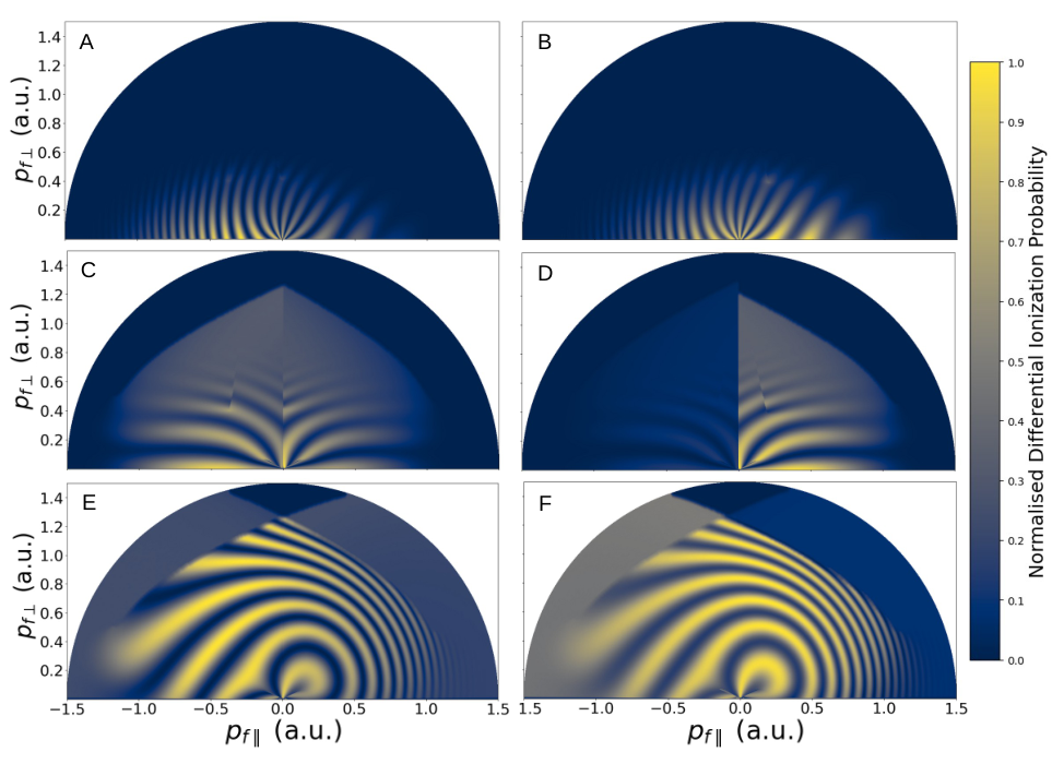
Next, in Fig. 11, we have a closer look at intra-cycle interference for fields of different parameters focusing on the CQSFA only. For clarity, we omit the prefactors associated with the stability of the orbit and the geometry of the state as they lead to additional momentum biases. They improve the agreement with ab-initio methods, but sometimes make the effect of quantum interference harder to dissect. We also restrict the ionization events to a single cycle, as the ATI rings can mask some holographic features. The figure shows holographic patterns for monochromatic fields [top row], and bichromatic (1,2) fields with the same relative phases as in the previous figures [middle and bottom rows]. In the left column, we consider a fixed unit cell starting at , while in the right column we perform an incoherent unit-cell averaging. This eliminates asymmetries due to including a finite range of ionization times, without leading to ATI rings, while fixed unit cells are useful for visualizing specific patterns. The value of determines the range of time from which saddle points are considered in the coherent sum by introducing an additional phase to the field. Saddle points from the range are taken for a field defined by where is the number of field cycles included.
Overall, in comparison with the monochromatic field, we see an enhancement of the spiral and spider around the axis and in the negative parallel momentum region for relative phase [Fig. 11(C)]. For [Fig. 11(E)], there is loss of contrast in the spiral and an enhancement in the spider for . If unit-cell averaging is performed, one sees that, for monochromatic fields, all patterns are symmetric with regard [see Fig. 11(B)]. This includes the interference carpet around the axis, which can be seen in the high-energy region of Fig. 11(B), the spider-like fringes close to the axis, and the fan-shaped distributions. This also holds for several features stemming from multi-path interference, such as the structures near the threshold where the fan and the spiral intersect. Once the second field is included, the patterns are no longer symmetric with regard to a reflection around , as a consequence of breaking the half-cycle symmetry. Moreover, for the carpet and other spiral-related features shift to the left, with an enhancement of the spider in the negative momentum region [Fig. 11(D)], while for these patterns shift to the right and the spider is more prominent for positive parallel momenta [Fig. 11(F)]. Furthermore, the interference carpet has high contrast for but not for [Figs. 11(E) and (F)], while the spider is sharper for and . Including prefactors mainly suppresses the spiral and enhances the yield near the polarization axis (see Figs. 9 and 10).

Due to the half-cycle symmetry being broken for the (1,2) field, we will employ a different orbit classification than in our previous publications [111, 113]. This classification is stated in Table 2, in which the orbits starting in the first half cycle will be indicated by a prime after their number, while for the orbits starting in the second half cycle this prime will be omitted. This classification will be used in the subsequent analysis. In Fig. 12, we plot the contributions from specific orbit pairs, working under the same assumptions as in Fig. 11. As a further approximation, we consider a specific unit cell starting at . This sheds more light on how specific patterns are affected.
| Orbit | |||
| + | + | + | |
| – | |||
| – | + | – | |
| + | |||
| – | – | – | |
| + | |||
| + | – | + | |
| – |
The upper panels of Fig. 12 display the fan-shaped pattern obtained with the interference of orbits 1 and 2. The intensity of the fan is asymmetric with regard to , being stronger on the left for [Fig. 12(A)], and on the right for [Fig. 12(B)]. However, this is a subtle effect, especially for . The intermediate panels show far more radical changes for the spider, which arises from the interference of orbits 2 and 3. For , the spider is slightly weaker for positive parallel momentum, but visible throughout [Fig. 12(C)], while for it is vanishingly small for negative parallel momentum and very strong for [Fig. 12(D)]. Finally, the main difference in the spiral-like fringes that result from the interference of orbits 3 and 4, when changing the relative phase from to , is the loss of contrast, which happens throughout but is more pronounced in the negative momentum region. This can be related to the fuzzy interference carpets that occur for in the averaged unit cell case [see Fig. 11(F)]. One should note that the carpet, or the spiral, is due to the interference of orbits that start at different half cycles. Changing the unit cell or considering an incoherent sum of unit cells just means that the start and end times for ionisation are being shifted. However, the ionisation probabilities and the time difference for events starting at different half cycles are still different. This difference will cause a loss of contrast.
| Structure | Sign of | Orbits | |
|---|---|---|---|
| Spider | |||
| Spiral | |||
| Fan | |||
The specific orbits, as classified in Table. 2, which contribute to each holographic pattern, in different momentum regions are tabulated in Table. 3. As in Table . 2, the prime indicates the orbits which start in the first half cycle. In order to clarify the behaviour of these interfering orbits, in Fig. 13, we plot the temporal profiles of the electric field, together with the imaginary parts of the ionization times (left and right columns, respectively) as functions of the final parallel momentum keeping the perpendicular momentum component fixed.
These times can be associated with the dominant term in , which dictates the ionization probability associated with a specific electron pathway. Because the ionization probability scales with , and the dominant term in the action is proportional to , the smaller is, the more probable tunneling will be. This will lead to a particular quantum pathway being prominent. For examples see [113, 114] in the context of photoelectron holography, as well as our previous work on laser-induced nonsequential double ionization [146, 147, 148, 149] and molecular high-order harmonic generation [150]. For interpreting the following picture, it is useful to note that an electron leaving at the peak of the field is expected to have vanishing momenta. In the SFA, also gives the most probable momentum for ionization to occur. However, due to the presence of the Coulomb potential the conservation of momentum is lost. This means, for instance, that an electron leaving with vanishing momentum along orbit 1 would be decelerated and trapped by the potential, while an electron leaving along orbit 2 or 3 would be accelerated by it. A more complete analysis of the final to initial momentum mapping is provided in our early work [111, 113, 114] (see also [151] for a forward momentum mapping, albeit with a different orbit classification). Here, however, we are interested in the final momenta as they will determine which trajectories contribute to the interference patterns.
For comparison, in the upper row of Fig. 13 the monochromatic-field scenario is displayed. The most pronounced feature is that, for a monochromatic field, the curves are symmetric around the axis. This is a consequence of the half-cycle symmetry of the field: the reflection corresponds to events displaced by half a cycle, for which, apart from a minus sign, the field and its gradient are identical [see Fig. 13(A)]. Still, the curves in Fig. 13(B) behave in distinct ways: For orbit 1, exhibits a single minimum at , orbits 2 and 3 exhibit minima at non-vanishing momenta and orbit 4 has a much flatter behaviour. These features have been discussed elsewhere [113] and are due to the orbits’ dynamics. Orbit 1 reaches the detector directly, and is decelerated by the binding potential, thus behaving similarly to its SFA counterpart. Orbits 2 and 3 are field-dressed hyperbolae, so that they are accelerated by the Coulomb potential when they are near the core. This renders the most probable final momentum non-vanishing. Finally, for orbit 4 is very small and much flatter, with regard to the electron momenta, than those for the other orbits. This happens because the ionization times associated with this orbit are located within a very narrow range around the maxima of the field. Therefore, the ionization probability associated with it will be high and vary much less with the electron momentum. For details see our recent manuscript [152].
The half-cycle symmetry is broken when the field is added (remaining panels), so that the imaginary parts associated with the orbits starting at different half cycles are no longer degenerate. Nonetheless, this behavior is different for and . For [Fig. 13(D)], this degeneracy is broken in two main ways. First, there are vertical shifts, due to the effective potential barriers being different, and a ‘tilting’ around associated to the field gradients being different around a field extremum, with trajectories starting at different half a cycle leading to strikingly different slopes in for . These features can be spotted very clearly around , and can be associated with the fields and corresponding ranges for , displayed in Fig. 13(C)]. The figure shows that, due to the reflection symmetry around the field zero crossing (), the field extrema remain the same up to a minus sign, while the field gradients around each field maxima or minima differ. This will lead to the different slopes in the imaginary parts of , but not so pronounced vertical shifts. In contrast, for , the vertical shifts in are much larger [Fig. 13(F)]. This is caused by the field extrema at consecutive half cycles having different amplitudes [see Fig. 13(E)]. However, the curves associated with processes starting at different half cycles look very similar, apart from a reflection around . This is due to the reflection symmetry around , which leads the field having the same gradient, in absolute value, around maxima or minima. The smaller displacement in for orbits starting at consecutive half cycles explains why the differences in intensity observed for the holographic patterns are subtler in the case.
Next, we analyse the behavior of specific holographic structures using Fig. 13. Fig. 13(F) suggests that, for , the contributions starting in the second half cycle will be strongly suppressed due to being large. This will lead to an extremely weak spider for , as it is associated with orbits 2 and 3 in Fig. 13(F). It will also cause a loss of contrast in the fan and the spiral, as those patterns result from the interference of pathways starting at different half cycles. For instance, in the region, the contributions of orbit and are very weakened. This means that, when orbit interferes with to form the fan, or when orbit interferes with to form the spiral, the interference fringes will be blurred. A similar argument can be used for the weakened orbit interfering with and for the suppressed orbit 4 interfering with , in the region. The suppression of the rescattering ridge for the positive parallel momentum region is also associated with being large for orbit . For , Fig. 13(D) shows that the asymmetries are subtler as they are caused by smaller shifts and by the field gradients around its extrema being different. For instance, the spiral and the spider are sharp and comparable throughout, with the spider (spiral) slightly stronger on the left (right). A noteworthy feature is the suppression of the fan’s contrast and strength for , due to the steeper gradients of orbits and and larger differences in in this region. Flatter, almost merging for and leads to a sharper contrast and a stronger fan for .

Due to the presence of the Coulomb potential, the above discussion only holds approximately. The interplay between the driving field and the Coulomb potential is highly non-trivial, and even small changes in the electron’s binding energy can lead to qualitatively different behaviors for the CQSFA (for a recent example see [117]).
5 Conclusions
In the present work, we perform a systematic analysis of the symmetries present in strong-field ionization with linearly polarized bichromatic fields of commensurate frequencies, and for what field frequency ratios and relative phases they are broken or retained. Apart from the well-known half-cycle symmetry, which is broken if is odd, there are temporal reflection symmetries around the field maxima and zero crossings. These three symmetries are always present for linearly polarized monochromatic fields. However, for fields this is not always the case. For instance, if is even, the half-cycle symmetry will not be broken, but, depending in the dephasing between both waves, the above-mentioned reflections may or may not hold. On the other hand, if the half-cycle symmetry is broken as in the case where is odd, at least one of the other two is broken as well. We provide explicit values for the relative phase for which symmetries exist, for a general linearly polarized field, together with the corresponding times for which they occur. This is performed in a saddle-point framework, and entails not only the real parts of the ionization times, but also their imaginary parts. This will have direct consequences in the contrast and prominence of holographic patterns.
We analyze these effects in the theoretical framework of the Coulomb quantum-orbit strong-field approximation (CQSFA), using saddle-point methods and investigating how the symmetries influence the existing ionization times and subsequent orbits. Saddle-point equations provide valuable insight not only on the real parts of the ionization times, which can be associated with electron orbits and their interference, but also on its imaginary parts, which are related to ionization probabilities and therefore clarify how prominent a specific process is. Furthermore, we provide an example of how symmetry breaking influence specific holographic patterns, such as the fan, the spider and the spiral, for fields. Throughout, we considered a weak high-frequency wave, so that the propagation in the continuum is minimally disrupted. Together with breaking the half-cycle symmetry, breaking at least one of the reflection symmetries mentioned above causes changes in contrast and/or strength for specific holographic patterns. If the reflection with regard to field zero crossing is unbroken, the field gradients will be different but the peaks will not differ in absolute value. This means that patterns starting in different half cycles will mostly retain their sharpness, but the spider will lose contrast, as it stems from orbits starting in the same half cycle. On the other hand, breaking the reflection with regard to the field peaks, will lead to loss of contrast in the fan and spiral, but the spider will remain sharp. However, it will lose intensity for the half cycle in which the field is weaker. These results also show that the orbit classification introduced in [142] is not sufficient to deal with linearly polarized fields that are not monochromatic or cannot be approximated by a monochromatic wave, and will depend on the field frequencies, relative intensities and relative phase. In the specific example provided here, eight types of orbits were necessary to interpret the CQSFA outcome.
A previous publication [77] has also reported alterations in the contrast of holographic patterns in two-color fields, which resulted from critical changes in tunnel ionization probabilities. These features were observed experimentally for argon atoms using a fundamental laser field with a wavelength of nm and an intensity . However, therein the main emphasis was on breaking the half-cycle symmetry, its influence on the spider and how this can be used for inferring ionization times. Furthermore, the standard SFA was used and the field was treated as a perturbation. Interestingly, similar effects to those in our work are reported, which suggest that the influence in ionization comes mainly from the laser field and its properties. Nonetheless, we show that the residual Coulomb potential plays an important role in determining the relevant sets of orbits and holographic patterns. We anticipate that, for bichromatic fields with driving waves of comparable intensities, the Coulomb potential will become even more important due to the presence of secondary, less prominent field maxima. They are expected to lead to other types of relevant orbits, which will be more critically affected by the potential. However, a detailed study of such features is beyond the scope of the present work. A key issue is to deal with the changes in the saddle-point contours and number of relevant orbits that occur in this parameter range, for a Coulomb-distorted approach such as the CQSFA. This may require the development of novel asymptotic approaches, apart from the uniform approximation for two nearly coalescent saddles that is widespread in strong-field physics [145]. Therefore, it is not clear whether the number, relevance and types of orbits can be determined for a general linearly polarized field of arbitrary frequency and intensity ratios, and relative phase. For experimental studies of photoelectron holography in two colour fields of comparable intensity see [105, 108].
Other important questions, which will be the topic of further investigations, are whether one may use tailored fields to manipulate holographic structures and thus extract information about the target which will not be available otherwise. A key difficulty is that some holographic patterns obfuscate others, so that the features of interest may be difficult to extract. For instance, the spider is quite prominent, such that, in early experiments, it was necessary to subtract its influence in order to see a subtler, fishbone structure [153, 154, 155]. The spider also obscures a spiral-like structure except close to the perpendicular momentum axis. The spiral arises from orbits that strongly interact with the core, and therefore is a promising holographic tool [101, 156]. Orthogonally polarized fields are potentially powerful tools for disentangling different types of intra-cycle interference, but their influence has been mostly interpreted using the Coulomb-free, standard SFA [51, 54]. The same holds for the understanding of dynamical symmetries of the field and the target: although there is a considerable body of work in this direction [55], the influence of the residual potential remains largely unexplored.
A key challenge is that the presence of residual potentials leads to deviations from the simple mapping dictated by the SFA. This has been pointed out for orthogonal two color fields [47], but is expected to happen as soon as the acceleration caused by the potential in the continuum becomes significant. Therefore, many of the arguments employed in the present work are approximate. If one is dealing with highly directional states or non-isotropic potentials, this becomes a non-trivial matter. In the SFA framework, aligning an axis of symmetry of the system with the field will guarantee that this symmetry is retained [55], while in the presence of the residual potential this will not necessarily hold. It is not yet clear how it will affect targets with specific geometries and/or internal degrees of freedom, which, per se, cause phase changes and modulations in holographic structures [157, 100, 158, 159, 160].
For instance, recently, we have found that the presence of a central potential may move the electron dynamics away from the polarization axis for orbit 4 [117], which led to a prominent rescattering ridge for excited Helium even if the initial bound state was oriented perpendicular to the driving-field polarization. This effect was extremely sensitive to the binding energy and the tunnel exit, and went against what one would expect from the physical intuition provided by the SFA. Furthermore, depending on the parity of the initial orbitals, some holographic structures will pick up extra phase differences. In order to assess that, one must minimize the continuum phase differences and Coulomb distortions by using a molecule and a companion atom with very similar ionization potentials [118].
If this is unclear for non-isotropic excited states in atoms, for molecules we expect this to be even more extreme. A molecular potential and also molecular orbitals are in general highly directional, with an angular dependency, symmetry axes, and other issues that critically affect holographic patterns. For instance, in [100] it was shown that the holographic structures are very sensitive with regard to the molecular orientation, which can be used to generate phase offsets. Signatures of different bound states [159] and nuclear-electronic coupling [160] also have a strong influence on photoelectron momentum distributions. A forward-backward asymmetry along the polarization vector for photoelectron spectra in can also be caused by the population of degenerate continuum states with opposite parities [157].
Specifically with regard to molecular systems and trajectory-based models, there may be intramolecular trajectories, which may move from one center to the other without reaching the continuum. Early high-order harmonic studies have shown that, even within the SFA these orbits may lead to quite prominent features [161]. In the presence of the binding potential, these orbits are expected to be chaotic or lead to resonances, population trapping and threshold effects. Other types of orbits may leave from one center and rescatter off the other [162, 150]. This may require a different orbit classification for the CQSFA orbits than that employed here. Finally, one should bear that the issues mentioned above are based on a highly simplified, one-electron picture. In reality, however, the core dynamics and multielectron effects must also be taken into consideration [163]. The present work is intended as a step towards the understanding of symmetry in a Coulomb-distorted context, an in providing a theoretical framework for a generic two-color linearly polarized field.
Acknowledgements: We would like to thank A. C. Bray and A. S. Maxwell for useful discussions. This work was partly funded by grant No. EP/J019143/1, from the UK Engineering and Physical Sciences Research Council (EPSRC). The authors acknowledge the use of the freely available QPROP software (www.qprop.de).
Appendix A Quantifying field asymmetries
In the specific case of a two-colour field, one may define asymmetry parameters in terms of how greatly the phase differs from the value of when the symmetry holds, or by using the corresponding electric field.
An example of a reasonable asymmetry parameter for the transformation is
| (51) |
This parameter vanishes if the field is symmetric upon , and is equivalent to a parameter defined just from the phase ,
| (52) |
where is the set of such that a specific symmetry holds, in the sense that inequalities are preserved when the parameters are interchanged [Fig. 14]. This means that for all , ,
| (53) |
This must hold by considering the conditions for symmetries to exist in Fig. 2 and the fact that sinusoidal functions vary monotonically between their zeroes and the midpoint of that zero and the adjacent zero. We illustrate both asymmetry parameters in Fig. 14, taking into consideration and a field. The figure shows that these parameters vanish for relative phase and , which is consistent with the symmetry upon the reflection holding for these phases. The parameter also reaches its maximum for , which is consistent with the discussion of Fig. 7.

Appendix B Determining saddle symmetries
The best way to discuss symmetries of the saddle-point solutions is to take some solution of equation (33), , and find some transformation of this solution such that the result of such transformations, , is equally a solution of equation (33).
First consider just the case where the pair have opposite parity so we consider phases such that . Take the complex conjugate of equation (33) to give
| (54) |
where the tilde denotes complex conjugation. By introducing the number , we can construct . For such that , and are equal to either plus or minus one. Likewise, if , will be either plus or minus 1. By multiplying by 1, equation (54) can be manipulated into the form
| (55) |
where and are a solution to the Diophantine equations
| (56) | |||||
| (57) |
By using the parities of and s to determine the parities of and for the cases odd, even and even, odd separately, we can determine in each case whether and are plus or minus one. By adjusting the form of the solution, (55) can be returned to the form of (33). The transformation of the solution required to do this is given by equation (58).
| (58) |
This can be returned to an expression which includes the saddle point time, by making the substitution . After some manipulations, we obtain
| (59) | |||||
| (60) |
where , are integer numbers. Equation (59) and (60) can be simplified further by solving the diophantine equations (56) and (57) in terms of the multiplicative inverse of modulo , .
| (61) | |||||
| (62) |
where .
Similar arguments can be made for which are both odd. However, in this case we additionally have the half cycle symmetry for all and the simple transformation
| (63) |
is also a solution to equation (33). In terms of saddle point times equation (63) becomes
| (64) | |||||
| (65) |
Now, for such that the following transformation gives another solution of equation (33), namely
| (66) |
This is found in the same way as the opposite parity case by multiplying by one and introducing the same , , as before. This strategy can be used to define the transformation of in equation (66), which leaves equation (33) invariant. This corresponds to the saddle point times having the symmetries
| (67) | |||||
| (68) |
which as before can be simplified to
| (69) | |||||
| (70) |
References
- [1] Manfred Lein “Molecular imaging using recolliding electrons” In Journal of Physics B: Atomic, Molecular and Optical Physics 40.16, 2007, pp. R135 URL: http://stacks.iop.org/0953-4075/40/i=16/a=R01
- [2] Ferenc Krausz and Misha Ivanov “Attosecond physics” In Rev. Mod. Phys. 81 American Physical Society, 2009, pp. 163–234 DOI: 10.1103/RevModPhys.81.163
- [3] P Salières et al. “Imaging orbitals with attosecond and Ångström resolutions: toward attochemistry?” In Reports on Progress in Physics 75.6, 2012, pp. 062401 URL: http://stacks.iop.org/0034-4885/75/i=6/a=062401
- [4] Lukas Gallmann, Claudio Cirelli and Ursula Keller “Attosecond Science: Recent Highlights and Future Trends” PMID: 22404594 In Annual Review of Physical Chemistry 63.1, 2012, pp. 447–469 DOI: 10.1146/annurev-physchem-032511-143702
- [5] Pierre Agostini and Louis DiMauro “The physics of attosecond light pulses” In Reports on Progress in Physics 67.6, 2004, pp. 813 URL: http://stacks.iop.org/0034-4885/67/i=6/a=R01
- [6] Francesca Calegari et al. “Advances in attosecond science” In Journal of Physics B: Atomic, Molecular and Optical Physics 49.6, 2016, pp. 062001 URL: http://stacks.iop.org/0953-4075/49/i=6/a=062001
- [7] J Marangos “Development of high harmonic generation spectroscopy of organic molecules and biomolecules” In Journal of Physics B: Atomic, Molecular and Optical Physics 49.13, 2016, pp. 132001 URL: http://stacks.iop.org/0953-4075/49/i=13/a=132001
- [8] C. Figueira and A Maxwell “It is all about phases: ultrafast holographic photoelectron imaging” In Reports on Progress in Physics 83.3 IOP Publishing, 2020, pp. 034401 DOI: 10.1088/1361-6633/ab5c91
- [9] P.. Corkum “Plasma perspective on strong field multiphoton ionization” In Phys. Rev. Lett. 71 American Physical Society, 1993, pp. 1994–1997 DOI: 10.1103/PhysRevLett.71.1994
- [10] W Becker, S Goreslavski, D Milošević and G Paulus “The plateau in above-threshold ionization: the keystone of rescattering physics” In Journal of Physics B: Atomic, Molecular and Optical Physics 51.16, 2018, pp. 162002 URL: http://stacks.iop.org/0953-4075/51/i=16/a=162002
- [11] W. Becker et al. “Above-threshold ionization: From classical features to quantum effects” In Advances in Atomic Molecular and Optical Physics 48, 2002, pp. 35–98 DOI: 10.1016/S1049-250X(02)80006-4
- [12] D Milošević, G Paulus, D Bauer and W Becker “Above-threshold ionization by few-cycle pulses” In Journal of Physics B: Atomic, Molecular and Optical Physics 39.14, 2006, pp. R203 URL: http://stacks.iop.org/0953-4075/39/i=14/a=R01
- [13] C. Figueira and X. Liu “Electron–electron correlation in strong laser fields” In Journal of Modern Optics 58.13, 2011, pp. 1076–1131 DOI: 10.1080/09500340.2010.543958
- [14] Wilhelm Becker, XiaoJun Liu, Phay Ho and Joseph. Eberly “Theories of photoelectron correlation in laser-driven multiple atomic ionization” In Rev. Mod. Phys. 84 American Physical Society, 2012, pp. 1011–1043 DOI: 10.1103/RevModPhys.84.1011
- [15] M. Lewenstein et al. “Theory of high-harmonic generation by low-frequency laser fields” In Phys. Rev. A 49 American Physical Society, 1994, pp. 2117–2132 DOI: 10.1103/PhysRevA.49.2117
- [16] Thomas Brabec and Ferenc Krausz “Intense few-cycle laser fields: Frontiers of nonlinear optics” In Rev. Mod. Phys. 72 American Physical Society, 2000, pp. 545–591 DOI: 10.1103/RevModPhys.72.545
- [17] Fritz Ehlotzky “Atomic phenomena in bichromatic laser fields” In Physics Reports 345.4, 2001, pp. 175–264 DOI: https://doi.org/10.1016/S0370-1573(00)00100-9
- [18] D Milošević, G Paulus, D Bauer and W Becker “Above-threshold ionization by few-cycle pulses” In Journal of Physics B: Atomic, Molecular and Optical Physics 39.14 IOP Publishing, 2006, pp. R203–R262 DOI: 10.1088/0953-4075/39/14/r01
- [19] N. Dudovich et al. “Measuring and controlling the birth of attosecond XUV pulses” In Nature Physics 2.11, 2006, pp. 781–786 DOI: 10.1038/nphys434
- [20] G. Doumy et al. “Attosecond Synchronization of High-Order Harmonics from Midinfrared Drivers” In Phys. Rev. Lett. 102 American Physical Society, 2009, pp. 093002 DOI: 10.1103/PhysRevLett.102.093002
- [21] J.. Dahlström et al. “Atomic and macroscopic measurements of attosecond pulse trains” In Phys. Rev. A 80 American Physical Society, 2009, pp. 033836 DOI: 10.1103/PhysRevA.80.033836
- [22] P. Eckle et al. “Attosecond Ionization and Tunneling Delay Time Measurements in Helium” In Science 322.5907 American Association for the Advancement of Science, 2008, pp. 1525–1529 DOI: 10.1126/science.1163439
- [23] Adrian. Pfeiffer et al. “Attoclock reveals natural coordinates of the laser-induced tunnelling current flow in atoms” In Nature Physics 8 Nature Publishing Group SN -, 2012, pp. 76–80 URL: https://doi.org/10.1038/nphys2125
- [24] A.. Pfeiffer et al. “Probing the Longitudinal Momentum Spread of the Electron Wave Packet at the Tunnel Exit” In Phys. Rev. Lett. 109 American Physical Society, 2012, pp. 083002 DOI: 10.1103/PhysRevLett.109.083002
- [25] Dror Shafir et al. “Resolving the time when an electron exits a tunnelling barrier” In Nature 485.7398, 2012, pp. 343–346 DOI: 10.1038/nature11025
- [26] Min Li et al. “Subcycle Dynamics of Coulomb Asymmetry in Strong Elliptical Laser Fields” In Phys. Rev. Lett. 111 American Physical Society, 2013, pp. 023006 DOI: 10.1103/PhysRevLett.111.023006
- [27] Jing Zhao and Manfred Lein “Determination of Ionization and Tunneling Times in High-Order Harmonic Generation” In Phys. Rev. Lett. 111 American Physical Society, 2013, pp. 043901 DOI: 10.1103/PhysRevLett.111.043901
- [28] I.. Ivanov and A.. Kheifets “Strong-field ionization of He by elliptically polarized light in attoclock configuration” In Phys. Rev. A 89 American Physical Society, 2014, pp. 021402 DOI: 10.1103/PhysRevA.89.021402
- [29] O. Pedatzur et al. “Attosecond tunnelling interferometry” In Nature Physics 11 Nature Publishing Group SN -, 2015, pp. 815–819 URL: https://doi.org/10.1038/nphys3436
- [30] Meng Han, Min Li, Ming-Ming Liu and Yunquan Liu “Tunneling wave packets of atoms from intense elliptically polarized fields in natural geometry” In Phys. Rev. A 95 American Physical Society, 2017, pp. 023406 DOI: 10.1103/PhysRevA.95.023406
- [31] A Landsman et al. “Rydberg state creation by tunnel ionization” In New Journal of Physics 15.1 IOP Publishing, 2013, pp. 013001 DOI: 10.1088/1367-2630/15/1/013001
- [32] Lisa Torlina et al. “Interpreting attoclock measurements of tunnelling times” In Nature Physics 11 Nature Publishing Group SN -, 2015, pp. 503–508 URL: https://doi.org/10.1038/nphys3340
- [33] Jost Henkel and Manfred Lein “Analysis of electron trajectories with two-color strong-field ionization” In Phys. Rev. A 92 American Physical Society, 2015, pp. 013422 DOI: 10.1103/PhysRevA.92.013422
- [34] Michael Klaiber, Karen. Hatsagortsyan and Christoph. Keitel “Under-the-Tunneling-Barrier Recollisions in Strong-Field Ionization” In Phys. Rev. Lett. 120 American Physical Society, 2018, pp. 013201 DOI: 10.1103/PhysRevLett.120.013201
- [35] Nicolas Eicke and Manfred Lein “Attoclock with counter-rotating bicircular laser fields” In Phys. Rev. A 99 American Physical Society, 2019, pp. 031402 DOI: 10.1103/PhysRevA.99.031402
- [36] Olga Smirnova, Yann Mairesse and Serguei Patchkovskii “Opportunities for chiral discrimination using high harmonic generation in tailored laser fields” In Journal of Physics B: Atomic, Molecular and Optical Physics 48.23 IOP Publishing, 2015, pp. 234005 DOI: 10.1088/0953-4075/48/23/234005
- [37] David Ayuso, Piero Decleva, Serguei Patchkovskii and Olga Smirnova “Chiral dichroism in bi-elliptical high-order harmonic generation” In Journal of Physics B: Atomic, Molecular and Optical Physics 51.6 IOP Publishing, 2018, pp. 06LT01 DOI: 10.1088/1361-6455/aaae5e
- [38] David Ayuso, Piero Decleva, Serguei Patchkovskii and Olga Smirnova “Strong-field control and enhancement of chiral response in bi-elliptical high-order harmonic generation: an analytical model” In Journal of Physics B: Atomic, Molecular and Optical Physics 51.12 IOP Publishing, 2018, pp. 124002 DOI: 10.1088/1361-6455/aabc95
- [39] Denitsa Baykusheva and Hans Wörner “Chiral Discrimination through Bielliptical High-Harmonic Spectroscopy” In Phys. Rev. X 8 American Physical Society, 2018, pp. 031060 DOI: 10.1103/PhysRevX.8.031060
- [40] A.. Maxwell et al. “Manipulating twisted electrons in strong-field ionization” In Faraday Discuss. 228 The Royal Society of Chemistry, 2021, pp. 394–412 DOI: 10.1039/D0FD00105H
- [41] S. Skruszewicz et al. “Two-Color Strong-Field Photoelectron Spectroscopy and the Phase of the Phase” In Phys. Rev. Lett. 115 American Physical Society, 2015, pp. 043001 DOI: 10.1103/PhysRevLett.115.043001
- [42] M Almajid et al. “Two-color phase-of-the-phase spectroscopy in the multiphoton regime” In Journal of Physics B: Atomic, Molecular and Optical Physics 50.19 IOP Publishing, 2017, pp. 194001 DOI: 10.1088/1361-6455/aa896a
- [43] D. Würzler et al. “Accurate retrieval of ionization times by means of the phase-of-the-phase spectroscopy, and its limits” In Phys. Rev. A 101 American Physical Society, 2020, pp. 033416 DOI: 10.1103/PhysRevA.101.033416
- [44] V.. Tulsky, M.. Almajid and D. Bauer “Two-color phase-of-the-phase spectroscopy with circularly polarized laser pulses” In Phys. Rev. A 98 American Physical Society, 2018, pp. 053433 DOI: 10.1103/PhysRevA.98.053433
- [45] V Tulsky, B Krebs, J Tiggesbäumker and D Bauer “Revealing laser-coherent electron features using phase-of-the-phase spectroscopy” In Journal of Physics B: Atomic, Molecular and Optical Physics 53.7 IOP Publishing, 2020, pp. 074001 DOI: 10.1088/1361-6455/ab69ab
- [46] Alexandra Landsman and Ursula Keller “Tunnelling time in strong field ionisation” In Journal of Physics B: Atomic, Molecular and Optical Physics 47.20, 2014, pp. 204024 URL: http://stacks.iop.org/0953-4075/47/i=20/a=204024
- [47] Li Zhang et al. “Laser-sub-cycle two-dimensional electron-momentum mapping using orthogonal two-color fields” In Phys. Rev. A 90 American Physical Society, 2014, pp. 061401 DOI: 10.1103/PhysRevA.90.061401
- [48] Martin Richter et al. “Streaking temporal double slit interference by an orthogonal two-color laser field” In J. Phys. Conf. Ser. 635.9, 2015, pp. 143001 DOI: 10.1088/1742-6596/635/9/092036
- [49] T. Das, B.. Augstein and C. Figueira “High-order-harmonic generation from diatomic molecules in driving fields with nonvanishing ellipticity: A generalized interference condition” In Phys. Rev. A 88 American Physical Society, 2013, pp. 023404 DOI: 10.1103/PhysRevA.88.023404
- [50] T. Das et al. “Extracting an electron’s angle of return from shifted interference patterns in macroscopic high-order-harmonic spectra of diatomic molecules” In Phys. Rev. A 92 American Physical Society, 2015, pp. 023406 DOI: 10.1103/PhysRevA.92.023406
- [51] Yang Li et al. “Identifying backward-rescattering photoelectron hologram with orthogonal two-color laser fields” In Opt. Express 24.21 OSA, 2016, pp. 23697–23706 DOI: 10.1364/OE.24.023697
- [52] Meng Han et al. “Revealing the Sub-Barrier Phase using a Spatiotemporal Interferometer with Orthogonal Two-Color Laser Fields of Comparable Intensity” In Phys. Rev. Lett. 119 American Physical Society, 2017, pp. 073201 DOI: 10.1103/PhysRevLett.119.073201
- [53] Xiaochun Gong et al. “Energy-Resolved Ultrashort Delays of Photoelectron Emission Clocked by Orthogonal Two-Color Laser Fields” In Phys. Rev. Lett. 118 American Physical Society, 2017, pp. 143203 DOI: 10.1103/PhysRevLett.118.143203
- [54] Xinhua Xie et al. “Disentangling Intracycle Interferences in Photoelectron Momentum Distributions Using Orthogonal Two-Color Laser Fields” In Phys. Rev. Lett. 119 American Physical Society, 2017, pp. 243201 DOI: 10.1103/PhysRevLett.119.243201
- [55] Dino Habibović, Wilhelm Becker and Dejan. Milošević “Symmetries and Selection Rules of the Spectra of Photoelectrons and High-Order Harmonics Generated by Field-Driven Atoms and Molecules” In Symmetry 13.9, 2021, pp. 1566 DOI: 10.3390/sym13091566
- [56] Dejan. Milošević, Wilhelm Becker and Richard Kopold “Generation of circularly polarized high-order harmonics by two-color coplanar field mixing” In Phys. Rev. A 61 American Physical Society, 2000, pp. 063403 DOI: 10.1103/PhysRevA.61.063403
- [57] D.. Milošević and W. Becker “Improved strong-field approximation and quantum-orbit theory: Application to ionization by a bicircular laser field” In Phys. Rev. A 93 American Physical Society, 2016, pp. 063418 DOI: 10.1103/PhysRevA.93.063418
- [58] Christopher. Mancuso et al. “Controlling electron-ion rescattering in two-color circularly polarized femtosecond laser fields” In Phys. Rev. A 93 American Physical Society, 2016, pp. 053406 DOI: 10.1103/PhysRevA.93.053406
- [59] Van-Hung Hoang, Van-Hoang Le, C.. Lin and Anh-Thu Le “Retrieval of target structure information from laser-induced photoelectrons by few-cycle bicircular laser fields” In Phys. Rev. A 95 American Physical Society, 2017, pp. 031402 DOI: 10.1103/PhysRevA.95.031402
- [60] S. Eckart et al. “Subcycle interference upon tunnel ionization by counter-rotating two-color fields” In Phys. Rev. A 97 American Physical Society, 2018, pp. 041402 DOI: 10.1103/PhysRevA.97.041402
- [61] D.. Milošević and W. Becker “Channel-closing effects in strong-field ionization by a bicircular field” In Journal of Physics B: Atomic, Molecular and Optical Physics 51.5, 2018, pp. 054001 URL: http://stacks.iop.org/0953-4075/51/i=5/a=054001
- [62] Shengjun Yue, Simon Brennecke, Hongchuan Du and Manfred Lein “Probing dynamical symmetries by bicircular high-order harmonic spectroscopy beyond the Born-Oppenheimer approximation” In Phys. Rev. A 101 American Physical Society, 2020, pp. 053438 DOI: 10.1103/PhysRevA.101.053438
- [63] S. Rozen et al. “Controlling Subcycle Optical Chirality in the Photoionization of Chiral Molecules” In Phys. Rev. X 9 American Physical Society, 2019, pp. 031004 DOI: 10.1103/PhysRevX.9.031004
- [64] Emilio Pisanty et al. “Knotting fractional-order knots with the polarization state of light” In Nature Photonics 13.8, 2019, pp. 569–574 DOI: 10.1038/s41566-019-0450-2
- [65] M. Busuladžić, A. Gazibegović-Busuladžić and D.. Milošević “Strong-field ionization of homonuclear diatomic molecules by a bicircular laser field: Rotational and reflection symmetries” In Phys. Rev. A 95 American Physical Society, 2017, pp. 033411 DOI: 10.1103/PhysRevA.95.033411
- [66] Ofer Neufeld, Daniel Podolsky and Oren Cohen “Floquet group theory and its application to selection rules in harmonic generation” In Nature Communications 10.1, 2019, pp. 405 DOI: 10.1038/s41467-018-07935-y
- [67] Ofir. Alon, Vitali Averbukh and Nimrod Moiseyev “Selection Rules for the High Harmonic Generation Spectra” In Phys. Rev. Lett. 80 American Physical Society, 1998, pp. 3743–3746 DOI: 10.1103/PhysRevLett.80.3743
- [68] D.. Milošević “Circularly polarized high harmonics generated by a bicircular field from inert atomic gases in the state: A tool for exploring chirality-sensitive processes” In Phys. Rev. A 92 American Physical Society, 2015, pp. 043827 DOI: 10.1103/PhysRevA.92.043827
- [69] J.. Ngoko Djiokap et al. “Electron Vortices in Photoionization by Circularly Polarized Attosecond Pulses” In Phys. Rev. Lett. 115, 2015, pp. 113004 DOI: 10.1103/PhysRevLett.115.113004
- [70] T. Bayer, Ch. Philipp, K. Eickhoff and M. Wollenhaupt “Atomic photoionization dynamics in ultrashort cycloidal laser fields” In Phys. Rev. A 102 American Physical Society, 2020, pp. 013104 DOI: 10.1103/PhysRevA.102.013104
- [71] Yuxin Kang et al. “Conservation laws for electron vortices in strong-field ionisation” In The European Physical Journal D 75.7, 2021, pp. 199 DOI: 10.1140/epjd/s10053-021-00214-4
- [72] Xi Liu et al. “Selection rules of high-order-harmonic generation: Symmetries of molecules and laser fields” In Phys. Rev. A 94 American Physical Society, 2016, pp. 033410 DOI: 10.1103/PhysRevA.94.033410
- [73] Ingo Barth and Olga Smirnova “Nonadiabatic tunneling in circularly polarized laser fields: Physical picture and calculations” In Phys. Rev. A 84 American Physical Society, 2011, pp. 063415 DOI: 10.1103/PhysRevA.84.063415
- [74] Ingo Barth and Olga Smirnova “Nonadiabatic tunneling in circularly polarized laser fields. II. Derivation of formulas” In Phys. Rev. A 87 American Physical Society, 2013, pp. 013433 DOI: 10.1103/PhysRevA.87.013433
- [75] M.. Frolov, N.. Manakov, A.. Silaev and N.. Vvedenskii “Analytic description of high-order harmonic generation by atoms in a two-color laser field” In Phys. Rev. A 81 American Physical Society, 2010, pp. 063407 DOI: 10.1103/PhysRevA.81.063407
- [76] Markus Kitzler et al. “Angular encoding in attosecond recollision” In New Journal of Physics 10.2 IOP Publishing, 2008, pp. 025029 DOI: 10.1088/1367-2630/10/2/025029
- [77] G. Porat et al. “Attosecond time-resolved photoelectron holography” In Nature Communications 9.1, 2018, pp. 2805 DOI: 10.1038/s41467-018-05185-6
- [78] C. Figueira, M. Dörr, W. Becker and W. Sandner “Time-frequency analysis of two-color high-harmonic generation” In Phys. Rev. A 60 American Physical Society, 1999, pp. 1377–1384 DOI: 10.1103/PhysRevA.60.1377
- [79] C. Figueira, D.. Milošević and G.. Paulus “Phase-dependent effects in bichromatic high-order harmonic generation” In Phys. Rev. A 61 American Physical Society, 2000, pp. 063415 DOI: 10.1103/PhysRevA.61.063415
- [80] C. Figueira and M.. Du “Enhancement of bichromatic high-order-harmonic generation with a high-frequency field” In Phys. Rev. A 64 American Physical Society, 2001, pp. 023415 DOI: 10.1103/PhysRevA.64.023415
- [81] O. Raz, O. Pedatzur, B.. Bruner and N. Dudovich “Spectral caustics in attosecond science” In Nature Photonics 6.3, 2012, pp. 170–173 DOI: 10.1038/nphoton.2011.353
- [82] V.. Strelkov “Attosecond-pulse production using resonantly enhanced high-order harmonics” In Phys. Rev. A 94 American Physical Society, 2016, pp. 063420 DOI: 10.1103/PhysRevA.94.063420
- [83] D. Faccialà et al. “Probe of Multielectron Dynamics in Xenon by Caustics in High-Order Harmonic Generation” In Phys. Rev. Lett. 117 American Physical Society, 2016, pp. 093902 DOI: 10.1103/PhysRevLett.117.093902
- [84] K.. Hamilton, H.. van Hart and A.. Brown “Pulse-shape control of two-color interference in high-order-harmonic generation” In Phys. Rev. A 95 American Physical Society, 2017, pp. 013408 DOI: 10.1103/PhysRevA.95.013408
- [85] N.. Shvetsov-Shilovski, E. Räsänen, G.. Paulus and L.. Madsen “Asymmetric photoelectron momentum distributions due to quantum interference in strong-field ionization by a few-cycle pulse” In Phys. Rev. A 89 American Physical Society, 2014, pp. 043431 DOI: 10.1103/PhysRevA.89.043431
- [86] C.. Ooi, W.. Ho and A.. Bandrauk “Effects of ultrashort laser pulses on angular distributions of photoionization spectra” In Scientific Reports 7.1, 2017, pp. 6739 DOI: 10.1038/s41598-017-05915-8
- [87] Sebastián. López and Diego. Arbó “Holographic interference in atomic photoionization from a semiclassical standpoint” In Physical Review A 100.2, 2019 DOI: 10.1103/physreva.100.023419
- [88] Sebastián. López and Diego. Arbó “Holographic interferences in Photoelectron Spectra: Different Approaches” In The European Physical Journal D 73.2, 2019 DOI: 10.1140/epjd/e2018-90528-5
- [89] A Rudenko et al. “Resonant structures in the low-energy electron continuum for single ionization of atoms in the tunnelling regime” In Journal of Physics B: Atomic, Molecular and Optical Physics 37.24, 2004, pp. L407 URL: http://stacks.iop.org/0953-4075/37/i=24/a=L03
- [90] C Maharjan et al. “Wavelength dependence of momentum-space images of low-energy electrons generated by short intense laser pulses at high intensities” In Journal of Physics B: At. Mol. Opt. Phys. 39.8, 2006, pp. 1955–1964 DOI: 10.1088/0953-4075/39/8/013
- [91] R. Gopal et al. “Three-Dimensional Momentum Imaging of Electron Wave Packet Interference in Few-Cycle Laser Pulses” In Phys. Rev. Lett. 103 American Physical Society, 2009, pp. 053001 DOI: 10.1103/PhysRevLett.103.053001
- [92] Zhangjin Chen et al. “Analysis of two-dimensional photoelectron momentum spectra and the effect of the long-range Coulomb potential in single ionization of atoms by intense lasers” In Phys. Rev. A 74 American Physical Society, 2006, pp. 053405 DOI: 10.1103/PhysRevA.74.053405
- [93] D.. Arbó et al. “Interference oscillations in the angular distribution of laser-ionized electrons near ionization threshold” In Physical Review Letters 96.14, 2006 DOI: 10.1103/physrevlett.96.143003
- [94] Y Huismans et al. “Time-Resolved Holography” In Science 331.6013, 2011, pp. 61–65 DOI: 10.1126/science.1198450
- [95] Xue-Bin Bian et al. “Subcycle interference dynamics of time-resolved photoelectron holography with midinfrared laser pulses” In Phys. Rev. A 84 American Physical Society, 2011, pp. 043420 DOI: 10.1103/PhysRevA.84.043420
- [96] Y. Huismans et al. “Scaling Laws for Photoelectron Holography in the Midinfrared Wavelength Regime” In Phys. Rev. Lett. 109 American Physical Society, 2012, pp. 013002 DOI: 10.1103/PhysRevLett.109.013002
- [97] T. Marchenko, Y. Huismans, K.. Schafer and M… Vrakking “Criteria for the observation of strong-field photoelectron holography” In Phys. Rev. A 84 American Physical Society, 2011, pp. 053427 DOI: 10.1103/PhysRevA.84.053427
- [98] Daniel. Hickstein et al. “Direct Visualization of Laser-Driven Electron Multiple Scattering and Tunneling Distance in Strong-Field Ionization” In Phys. Rev. Lett. 109 American Physical Society, 2012, pp. 073004 DOI: 10.1103/PhysRevLett.109.073004
- [99] M. Möller et al. “Off-axis low-energy structures in above-threshold ionization” In Phys. Rev. A 90 American Physical Society, 2014, pp. 023412 DOI: 10.1103/PhysRevA.90.023412
- [100] M Meckel et al. “Signatures of the continuum electron phase in molecular strong-field photoelectron holography” In Nature Physics 10.8, 2014, pp. 594–600 URL: http://dx.doi.org/10.1038/nphys3010
- [101] Andrew. Maxwell et al. “Spiral-like holographic structures: Unwinding interference carpets of Coulomb-distorted orbits in strong-field ionization” In Phys. Rev. A 102 American Physical Society, 2020, pp. 033111 DOI: 10.1103/PhysRevA.102.033111
- [102] Peng Qin, Xufei Sun, Yunquan Liu and Zhanghai Chen “Revealing rescattering-induced subcycle dynamics of the spiral-like holographic structure” In Phys. Rev. A 104 American Physical Society, 2021, pp. 053111 DOI: 10.1103/PhysRevA.104.053111
- [103] Xinhua Xie “Two-Dimensional Attosecond Electron Wave-Packet Interferometry” In Phys. Rev. Lett. 114 American Physical Society, 2015, pp. 173003 DOI: 10.1103/PhysRevLett.114.173003
- [104] Meng Han et al. “Attoclock Photoelectron Interferometry with Two-Color Corotating Circular Fields to Probe the Phase and the Amplitude of Emitting Wave Packets” In Phys. Rev. Lett. 120 American Physical Society, 2018, pp. 073202 DOI: 10.1103/PhysRevLett.120.073202
- [105] Xinhua Xie et al. “Attosecond Probe of Valence-Electron Wave Packets by Subcycle Sculpted Laser Fields” In Phys. Rev. Lett. 108 American Physical Society, 2012, pp. 193004 DOI: 10.1103/PhysRevLett.108.193004
- [106] Xinhua Xie et al. “Probing the influence of the Coulomb field on atomic ionization by sculpted two-color laser fields” In New Journal of Physics 15.4 IOP Publishing, 2013, pp. 043050 DOI: 10.1088/1367-2630/15/4/043050
- [107] Diego. Arbó et al. “Interference of electron wave packets in atomic ionization by subcycle sculpted laser pulses” In Phys. Rev. A 89 American Physical Society, 2014, pp. 043414 DOI: 10.1103/PhysRevA.89.043414
- [108] D.. Arbó et al. “Ionization of argon by two-color laser pulses with coherent phase control” In Physical Review A 92.2, 2015 DOI: 10.1103/physreva.92.023402
- [109] Xinhua Xie et al. “Channel-resolved subcycle interferences of electron wave packets emitted from in two-color laser fields” In High Power Laser Science and Engineering 4 Cambridge University Press, 2016, pp. e40 DOI: 10.1017/hpl.2016.40
- [110] Siqiang Luo et al. “Angular-dependent asymmetries of above-threshold ionization in a two-color laser field” In Phys. Rev. A 96 American Physical Society, 2017, pp. 023417 DOI: 10.1103/PhysRevA.96.023417
- [111] X.. Lai, C. Poli, H. Schomerus and C. Figueira de Morisson Faria “Influence of the Coulomb potential on above-threshold ionization: A quantum-orbit analysis beyond the strong-field approximation” In Phys. Rev. A 92.4, 2015, pp. 043407 DOI: 10.1103/PhysRevA.92.043407
- [112] Xuanyang. Lai et al. “Near-threshold photoelectron holography beyond the strong-field approximation” In Phys. Rev. A 96.1, 2017, pp. 013414 DOI: 10.1103/PhysRevA.96.013414
- [113] A.. Maxwell, A. Al-Jawahiry, T. Das and C. Figueira “Coulomb-corrected quantum interference in above-threshold ionization: Working towards multi-trajectory electron holography” In Phys. Rev. A 96.2, 2017, pp. 023420 DOI: 10.1103/PhysRevA.96.023420
- [114] Andrew. Maxwell, A. Al-Jawahiry, X.. Lai and C. Figueira de Morisson Faria “Analytic quantum-interference conditions in Coulomb corrected photoelectron holography” In J. Phys. B At. Mol. Opt. Phys. 51.4, 2018, pp. 044004
- [115] A.. Maxwell and C. Figueira “Coulomb-free and Coulomb-distorted recolliding quantum orbits in photoelectron holography” In J. Phys. B At. Mol. Phys. 51 IOP Publishing, 2018, pp. 124001 arXiv: http://arxiv.org/abs/1802.00789
- [116] A.. Maxwell, S.. Popruzhenko and C. Figueira “Treating branch cuts in quantum trajectory models for photoelectron holography” In Phys. Rev. A 98 American Physical Society, 2018, pp. 063423 DOI: 10.1103/PhysRevA.98.063423
- [117] A Bray et al. “Polarization in strong-field ionization of excited helium” In Journal of Physics B: Atomic, Molecular and Optical Physics 54.19 IOP Publishing, 2021, pp. 194002 DOI: 10.1088/1361-6455/ac2e4a
- [118] HuiPeng Kang et al. “Holographic detection of parity in atomic and molecular orbitals” In Phys. Rev. A 102 American Physical Society, 2020, pp. 013109 DOI: 10.1103/PhysRevA.102.013109
- [119] Nicholas Werby et al. “Dissecting subcycle interference in photoelectron holography” In Phys. Rev. A 104 American Physical Society, 2021, pp. 013109 DOI: 10.1103/PhysRevA.104.013109
- [120] Dieter Bauer and Peter Koval “Qprop: A Schrödinger-solver for intense laser–atom interaction” In Computer Physics Communications 174.5, 2006, pp. 396–421 DOI: https://doi.org/10.1016/j.cpc.2005.11.001
- [121] Kasra Amini et al. “Symphony on strong field approximation” In Reports on Progress in Physics 82.11 IOP Publishing, 2019, pp. 116001 DOI: 10.1088/1361-6633/ab2bb1
- [122] Volker Mosert and Dieter Bauer “Photoelectron spectra with Qprop and t-SURFF” In Computer Physics Communications 207, 2016, pp. 452–463 DOI: https://doi.org/10.1016/j.cpc.2016.06.015
- [123] Vasily Tulsky and Dieter Bauer “Qprop with faster calculation of photoelectron spectra” In Computer Physics Communications 251, 2020, pp. 107098 DOI: https://doi.org/10.1016/j.cpc.2019.107098
- [124] Hagen Kleinert “Path Integrals in Quantum Mechanics, Statistics, Polymer Physics, and Financial Markets” World Scientific, 2009
- [125] D.. Milošević “Phase space path-integral formulation of the above-threshold ionization” In Journal of Mathematical Physics 54.4, 2013, pp. 042101 DOI: 10.1063/1.4797476
- [126] Misha Ivanov, Michael Spanner and Olga Smirnova “Anatomy of strong field ionization” In Journal of Modern Optics 52.2-3 Taylor & Francis, 2005, pp. 165–184 DOI: 10.1080/0950034042000275360
- [127] S Popruzhenko “Keldysh theory of strong field ionization: history, applications, difficulties and perspectives” In Journal of Physics B: Atomic, Molecular and Optical Physics 47.20, 2014, pp. 204001 URL: http://stacks.iop.org/0953-4075/47/i=20/a=204001
- [128] M. Lewenstein, K.. Kulander, K.. Schafer and P.. Bucksbaum “Rings in above-threshold ionization: A quasiclassical analysis” In Phys. Rev. A 51 American Physical Society, 1995, pp. 1495–1507 DOI: 10.1103/PhysRevA.51.1495
- [129] A. Lohr, M. Kleber, R. Kopold and W. Becker “Above-threshold ionization in the tunneling regime” In Phys. Rev. A 55 American Physical Society, 1997, pp. R4003–R4006 DOI: 10.1103/PhysRevA.55.R4003
- [130] W. Becker, A. Lohr, M. Kleber and M. Lewenstein “A unified theory of high-harmonic generation: Application to polarization properties of the harmonics” In Phys. Rev. A 56 American Physical Society, 1997, pp. 645–656 DOI: 10.1103/PhysRevA.56.645
- [131] L.V. Keldysh “Ionization in the field of a strong electromagnetic wave” In Sov. Phys. JETP 20, 1965, pp. 1307
- [132] F Faisal “Multiple absorption of laser photons by atoms” In Journal of Physics B: Atomic and Molecular Physics 6.4, 1973, pp. L89 URL: http://stacks.iop.org/0022-3700/6/i=4/a=011
- [133] Howard. Reiss “Effect of an intense electromagnetic field on a weakly bound system” In Phys. Rev. A 22 American Physical Society, 1980, pp. 1786–1813 DOI: 10.1103/PhysRevA.22.1786
- [134] S.V. Popruzhenko and D. Bauer “Strong field approximation for systems with Coulomb interaction” In Journal of Modern Optics 55.16 Taylor & Francis, 2008, pp. 2573–2589 DOI: 10.1080/09500340802161881
- [135] Tian-Min Yan and D. Bauer “Sub-barrier Coulomb effects on the interference pattern in tunneling-ionization photoelectron spectra” In Phys. Rev. A 86.5, 2012, pp. 053403 DOI: 10.1103/PhysRevA.86.053403
- [136] Lisa Torlina and Olga Smirnova “Time-dependent analytical -matrix approach for strong-field dynamics. I. One-electron systems” In Phys. Rev. A 86 American Physical Society, 2012, pp. 043408 DOI: 10.1103/PhysRevA.86.043408
- [137] Lisa Torlina, Jivesh Kaushal and Olga Smirnova “Time-resolving electron-core dynamics during strong-field ionization in circularly polarized fields” In Phys. Rev. A 88 American Physical Society, 2013, pp. 053403 DOI: 10.1103/PhysRevA.88.053403
- [138] Lisa Torlina, Felipe Morales, H.. Muller and Olga Smirnova “Ab initio verification of the analytical R-matrix theory for strong field ionization” In J. Phys. B At. Mol. Opt. Phys. 47 IOP Publishing, 2014, pp. 204021 DOI: 10.1088/0953-4075/47/20/204021
- [139] S.. Popruzhenko “Invariant form of Coulomb corrections in the theory of nonlinear ionization of atoms by intense laser radiation” In J. Exp. Theor. Phys. 118.4, 2014, pp. 580–586 DOI: 10.1134/S1063776114040062
- [140] Emilio Pisanty and Misha Ivanov “Slalom in complex time: Emergence of low-energy structures in tunnel ionization via complex-time contours” In Phys. Rev. A 93.4, 2016, pp. 1–17 DOI: 10.1103/PhysRevA.93.043408
- [141] C Zagoya et al. “Quantum and semiclassical phase-space dynamics of a wave packet in strong fields using initial-value representations” In New Journal of Physics 16.10, 2014, pp. 103040 URL: http://stacks.iop.org/1367-2630/16/i=10/a=103040
- [142] Tian-Min Yan, S.. Popruzhenko, M… Vrakking and D. Bauer “Low-Energy Structures in Strong Field Ionization Revealed by Quantum Orbits” In Phys. Rev. Lett. 105 American Physical Society, 2010, pp. 253002 DOI: 10.1103/PhysRevLett.105.253002
- [143] A Jašarević et al. “Application of the saddle-point method to strong-laser-field ionization” In Journal of Physics A: Mathematical and Theoretical 53.12 IOP Publishing, 2020, pp. 125201 DOI: 10.1088/1751-8121/ab749b
- [144] J. Gallian “Contemporary abstract algebra” Brooks Cole, 2016, pp. pp.446–452
- [145] C. Figueira, H. Schomerus and W. Becker “High-order above-threshold ionization: The uniform approximation and the effect of the binding potential” In Phys. Rev. A 66 American Physical Society, 2002, pp. 043413 DOI: 10.1103/PhysRevA.66.043413
- [146] X. Liu and C. Figueira “Nonsequential Double Ionization with Few-Cycle Laser Pulses” In Phys. Rev. Lett. 92 American Physical Society, 2004, pp. 133006 DOI: 10.1103/PhysRevLett.92.133006
- [147] C. Figueira, X. Liu, A. Sanpera and M. Lewenstein “Classical and quantum-mechanical treatments of nonsequential double ionization with few-cycle laser pulses” In Phys. Rev. A 70 American Physical Society, 2004, pp. 043406 DOI: 10.1103/PhysRevA.70.043406
- [148] C. Figueira “Laser-induced nonsequential double ionization in diatomic molecules: one- and two-centre rescattering scenarios” In Journal of Physics B: Atomic, Molecular and Optical Physics 42.10 IOP Publishing, 2009, pp. 105602 DOI: 10.1088/0953-4075/42/10/105602
- [149] C. Figueira, T. Shaaran and M.. Nygren “Time-delayed nonsequential double ionization with few-cycle laser pulses: Importance of the carrier-envelope phase” In Phys. Rev. A 86 American Physical Society, 2012, pp. 053405 DOI: 10.1103/PhysRevA.86.053405
- [150] C. Figueira “High-order harmonic generation in diatomic molecules: A quantum-orbit analysis of the interference patterns” In Phys. Rev. A 76 American Physical Society, 2007, pp. 043407 DOI: 10.1103/PhysRevA.76.043407
- [151] Min Li et al. “Classical-Quantum Correspondence for Above-Threshold Ionization” In Phys. Rev. Lett. 112 American Physical Society, 2014, pp. 113002 DOI: 10.1103/PhysRevLett.112.113002
- [152] Nicholas Werby et al. “Time Correlation Filtering Reveals Two-Path Electron Quantum Interference in Strong-Field Ionization” In arXiv.2205.07166 [physics.atom-ph] arXiv, 2022 URL: https://arxiv.org/abs/2205.07166
- [153] Xue-Bin Bian and André. Bandrauk “Attosecond Time-Resolved Imaging of Molecular Structure by Photoelectron Holography” In Phys. Rev. Lett. 108 American Physical Society, 2012, pp. 263003 DOI: 10.1103/PhysRevLett.108.263003
- [154] Marko Haertelt et al. “Probing Molecular Dynamics by Laser-Induced Backscattering Holography” In Phys. Rev. Lett. 116.13, 2016, pp. 133001 DOI: 10.1103/PhysRevLett.116.133001
- [155] Min Li et al. “Revealing backward rescattering photoelectron interference of molecules in strong infrared laser fields” In Sci. Rep. 5, 2015, pp. 8519 DOI: 10.1038/srep08519
- [156] Peng Qin, Xufei Sun, Yunquan Liu and Zhanghai Chen “Revealing rescattering-induced subcycle dynamics of the spiral-like holographic structure” In Phys. Rev. A 104 American Physical Society, 2021, pp. 053111 DOI: 10.1103/PhysRevA.104.053111
- [157] J Fernández and L Madsen “Energy-resolved photoelectron angular distributions of in intense femtosecond laser pulses” In Journal of Physics B: Atomic, Molecular and Optical Physics 42.2 IOP Publishing, 2009, pp. 021001 DOI: 10.1088/0953-4075/42/2/021001
- [158] Ming-Ming Liu et al. “Phase Structure of Strong-Field Tunneling Wave Packets from Molecules” In Phys. Rev. Lett. 116 American Physical Society, 2016, pp. 163004 DOI: 10.1103/PhysRevLett.116.163004
- [159] Mingrui He et al. “Direct Visualization of Valence Electron Motion Using Strong-Field Photoelectron Holography” In Phys. Rev. Lett. 120 American Physical Society, 2018, pp. 133204 DOI: 10.1103/PhysRevLett.120.133204
- [160] S.G Walt et al. “Dynamics of valence-shell electrons and nuclei probed by strong-field holography and rescattering” In Nat Commun 8, 2017, pp. 15651 DOI: 10.1038/ncomms15651
- [161] R. Kopold, W. Becker and M. Kleber “Model calculations of high-harmonic generation in molecular ions” In Phys. Rev. A 58 American Physical Society, 1998, pp. 4022–4038 DOI: 10.1103/PhysRevA.58.4022
- [162] C.. Chirilă and M. Lein “Strong-field approximation for harmonic generation in diatomic molecules” In Phys. Rev. A 73 American Physical Society, 2006, pp. 023410 DOI: 10.1103/PhysRevA.73.023410
- [163] Olga Smirnova et al. “High harmonic interferometry of multi-electron dynamics in molecules” In Nature 460.7258, 2009, pp. 972–977 DOI: 10.1038/nature08253