跳到论文正文
W Papers独立论文阅读器 arXiv:2203.02454 论文正文 计算阅读时间 · 0%
引用这篇论文根据当前论文元数据生成,正式投稿前建议核对。


License: CC BY 4.0
arXiv:2203.02454v2 [math-ph] 24 Mar 2022

Optimal parabolic upper bound for the energy-momentum relation of a strongly coupled polaron

David Mitrouskas, Krzysztof Myśliwy iand Robert Seiringer Thanks: Institute of Science and Technology Austria (ISTA), Am Campus 1, 3400 Klosterneuburg, Austria.
Email: david.mitrouskas@ist.ac.at
Thanks: Institute of Science and Technology Austria (ISTA), Am Campus 1, 3400 Klosterneuburg, Austria.
Email: krzysztof.mysliwy@ist.ac.at
Thanks: Institute of Science and Technology Austria (ISTA), Am Campus 1, 3400 Klosterneuburg, Austria.
Email: robert.seiringer@ist.ac.at
March 23, 2022
Abstract

We consider the large polaron described by the Fröhlich Hamiltonian and study its energy-momentum relation defined as the lowest possible energy as a function of the total momentum. Using a suitable family of trial states, we derive an optimal parabolic upper bound for the energy-momentum relation in the limit of strong coupling. The upper bound consists of a momentum independent term that agrees with the predicted two-term expansion for the ground state energy of the strongly coupled polaron at rest, and a term that is quadratic in the momentum with coefficient given by the inverse of twice the classical effective mass introduced by Landau and Pekar.

1 Introduction

1.1 The Model

The large polaron provides an idealized description for the motion of a slow band electron through a polarizable crystal. The analysis of the polaron is a classic problem in solid state physics that first appeared in 1933 when Landau introduced the idea of self-trapping of an electron in a polarizable environment [28]. Since it provides a simple model for a particle interacting with a nonrelativistic quantum field, the polaron has been of interest also in field theory and mathematical physics. In particular the strong coupling theory of the polaron and Pekar’s adiabatic approximation have been the source of interesting and challenging mathematical problems.

Following H. Fröhlich [20] the Hamiltonian of the model acts on the Hilbert space

ℋ=L2​(ℝ3,d​x)⊗ℱ,\displaystyle\mathscr{H}\,=\,L^{2}(\mathbb{R}^{3},\textnormal{d}x)\otimes\mathcal{F}, (1.1)

with ℱ\mathcal{F} the bosonic Fock space over L2​(ℝ3)L^{2}(\mathbb{R}^{3}), and is given by

Hα=−Δx+α−2​ℕ+α−1​ϕ​(hx).\displaystyle H_{\alpha}\,=\,-\Delta_{x}+\alpha^{-2}\mathbb{N}+\alpha^{-1}\phi(h_{x}). (1.2)

Here x∈ℝ3x\in\mathbb{R}^{3} is the coordinate of the electron, ℕ\mathbb{N} denotes the number operator on Fock space, and the field operator ϕ⁡(hx)=a†​(hx)+a⁡(hx)\phi(h_{x})=a^{\dagger}(h_{x})+a(h_{x}) with coupling function

hx​(y)=−12​π2​|x−y|2\displaystyle h_{x}(y)\,=\,-\frac{1}{2\pi^{2}|x-y|^{2}} (1.3)

accounts for the interaction between the electron and the quantum field. The creation and annihilation operators satisfy the usual canonical commutation relations

[a⁡(f),a†​(g)]=⟨f|g⟩L2,[a⁡(f),a⁡(g)]= 0.\displaystyle\big[a(f),a^{\dagger}(g)\big]\,=\,\big\langle f|g\big\rangle_{\text{\tiny{$L^{2}$}}},\quad\big[a(f),a(g)\big]\,=\,0. (1.4)

Since we set ℏ=1\hbar=1 and the mass of the electron equal to 1/21/2, the only free parameter is the coupling constant α>0\alpha>0.

By rescaling all lengths by a factor 1/α1/\alpha, one can show that α2​Hα\alpha^{2}H_{\alpha} is unitarily equivalent to the Hamiltonian

HαPolaron=−Δx+ℕ+α​ϕ​(hx),\displaystyle H_{\alpha}^{\rm{Polaron}}\,=\,-\Delta_{x}+\mathbb{N}+\sqrt{\alpha}\phi(h_{x}), (1.5)

which is more common in the polaron literature and also explains why α→∞\alpha\to\infty is called the strong coupling limit.

The Fröhlich Hamiltonian defines a translation invariant model, i.e., it commutes with the total momentum operator,

[Hα,−i​∇x+Pf]= 0\displaystyle[H_{\alpha},-i\nabla_{x}+P_{f}]\,=\,0 (1.6)

where Pf=dΓ(−i∇)P_{f}=\textnormal{d}\Gamma(-i\nabla) denotes the momentum operator of the phonons. This allows the definition of the energy-momentum relation Eα​(P)E_{\alpha}(P) as the lowest possible energy of HαH_{\alpha} when restricted to states with total momentum P∈ℝ3P\in\mathbb{R}^{3}. To this end, it is convenient to switch to the Lee–Low–Pines representation

Hα​(P)\displaystyle H_{\alpha}(P) =(Pf−P)2+α−2​ℕ+α−1​ϕ​(h0),\displaystyle\,=\,(P_{f}-P)^{2}+\alpha^{-2}\mathbb{N}+\alpha^{-1}\phi(h_{0}), (1.7)

where Hα​(P)H_{\alpha}(P) acts on the Fock space only [30]. The Fröhlich Hamiltonian HαH_{\alpha} is unitarily equivalent to the fiber decomposition ∫ℝ3⊕Hα​(P)​d​P\int^{\oplus}_{\mathbb{R}^{3}}H_{\alpha}(P)\textnormal{d}P, which follows easily from transforming HαH_{\alpha} with ei​Pf​xe^{iP_{f}x} and diagonalizing the obtained operator in the electron coordinate. The energy-momentum relation is then defined as the ground state energy of the fiber Hamiltonian,

Eα​(P)\displaystyle E_{\alpha}(P) =infσ​(Hα​(P)),\displaystyle\,=\,\inf\sigma(H_{\alpha}(P)), (1.8)

which by construction satisfies Eα​(R​P)=Eα​(P)E_{\alpha}(RP)=E_{\alpha}(P) for all rotations R∈SO​(3)R\in\textnormal{SO}(3). It is known that Eα​(0)≤Eα​(P)E_{\alpha}(0)\leq E_{\alpha}(P) and hence Eα​(0)=infσ⁡(Hα)E_{\alpha}(0)=\inf\sigma(H_{\alpha}) (in fact it is expected that Eα​(0)<Eα​(P)E_{\alpha}(0)<E_{\alpha}(P) for all P≠0P\neq 0 [12]). Further properties, such as the domain of analyticity, existence of ground states and the value of the bottom of the continuous spectrum, were analyzed in [21, 51, 42, 23, 10].

The aim of this work is to analyze the quantitative behavior of the energy-momentum relation for large coupling α→∞\alpha\to\infty. Our main result provides an upper bound for Eα​(P)E_{\alpha}(P). The upper bound consists of a momentum independent part coinciding with the optimal upper bound for the ground state energy of the strongly coupled polaron at rest, and a momentum dependent part. In more detail, the momentum independent part is given by the classical Pekar energy and the corresponding quantum fluctuations that are described by the energy of a system of harmonic oscillators with frequencies determined by the Hessian of the corresponding classical field functional. This part agrees with the expected asymptotic form of Eα​(0)E_{\alpha}(0), see (1.25). The momentum dependent part, on the other hand, describes the energy of a free particle with mass M⁡(α)=2​α43​∫|∇φ|2M(\alpha)=\frac{2\alpha^{4}}{3}\int|\nabla\varphi|^{2}, where φ\varphi denotes the self-consistent polarization field, which coincides with the classical polaron mass introduced by Landau and Pekar [29], see (1.24). As will be explained in Section 1.3, our result confirms the heuristic picture of the polaron (the electron and the accompanying classical field) as a free quasi-particle with largely enhanced mass. To our best knowledge, the upper bound we present in this work is the first rigorous result about the connection between the energy-momentum relation Eα​(P)E_{\alpha}(P) and the classical polaron mass M⁡(α)M(\alpha).

Starting from the works in the 30’s and 40’s [28, 29, 19] there has been a large number of publications in the physics literature that studied the ground state energy Eα​(0)E_{\alpha}(0) and the effective mass, that is, the inverse curvature of Eα​(P)E_{\alpha}(P) at P=0P=0. For a comprehensive summary of the earlier results, we refer to [39]. More recent developments are reviewed in [3]. Mathematically rigorous results for the leading order asymptotics of Eα​(0)E_{\alpha}(0), for α\alpha large, were obtained by Lieb and Yamazaki [38] (with non-matching upper and lower bounds) and by Donsker and Varadhan [11] as well as Lieb and Thomas [37]. The effective mass has been studied in [50, 12, 14, 36, 35, 6]. Further improvements have been obtained for confined polarons or polaron models with more regular interaction [18, 15, 45]. For completeness, let us also mention recent progress in the understanding of the polaron path measure [44, 5] as well as the increased interest in the analysis of the Schrödinger time evolution of strongly coupled polarons [25, 32, 33, 40, 13, 16, 17].

1.2 Pekar functionals

The semiclassical theory of the polaron has been introduced by Pekar [48]. It arises naturally in the context of strong coupling, based on the expectation that the electron and the phonons are adiabatically decoupled, similarly as the electrons are adiabatically decoupled from the heavy nuclei in the famous Born–Oppenheimer theory [8, 7]. With this in mind, one can minimize the Fröhlich Hamiltonian over product states of the form

Ψu,v=u⊗ea†​(α​v)​Ω\displaystyle\Psi_{u,v}\,=\,u\otimes e^{a^{\dagger}(\alpha v)}\Omega (1.9)

where u∈H1​(ℝ3)u\in H^{1}(\mathbb{R}^{3}) is a normalized electron wave function, Ω=(1,0,0,…)\Omega=(1,0,0,\ldots) the Fock space vacuum and ea†​(α​v)​Ωe^{a^{\dagger}(\alpha v)}\Omega the coherent state, up to normalization, that is associated with a classical field α​v∈L2​(ℝ3)\alpha v\in L^{2}(\mathbb{R}^{3}). A simple computation leads to the Pekar energy functional

𝒢⁡(u,v)=⟨Ψu,v|Hα​Ψu,v⟩ℋ⟨Ψu,v|Ψu,v⟩ℋ=⟨u|(−Δ+Vv)​u⟩L2+‖v‖L22\displaystyle\mathcal{G}(u,v)\,=\,\frac{\big\langle\Psi_{u,v}|H_{\alpha}\Psi_{u,v}\big\rangle_{\text{\tiny{$\mathscr{H}$}}}}{\big\langle\Psi_{u,v}|\Psi_{u,v}\big\rangle_{\text{\tiny{$\mathscr{H}$}}}}\,=\,\big\langle u|(-\Delta+V^{v})u\big\rangle_{\text{\tiny{$L^{2}$}}}+|\hskip-1.0pt|v|\hskip-1.0pt|^{2}_{\text{\tiny{$L^{2}$}}} (1.10)

with polarization potential

Vv(x)=−2Re⟨v|hx⟩L2=−Re∫v⁡(y)π2​|x−y|2dy.\displaystyle V^{v}(x)\,=\,-2\operatorname{Re}\big\langle v|h_{x}\big\rangle_{\text{\tiny{$L^{2}$}}}\,=\,-\operatorname{Re}\int\frac{v(y)}{\pi^{2}|x-y|^{2}}\textnormal{d}y. (1.11)

By completing the square, one can further remove the field variable and obtain the energy functional for the electron wave function,

ℰ⁡(u)\displaystyle\mathcal{E}(u) =infv∈L2𝒢⁡(u,v)=∫|u⁡(x)|2​d​x−14​π​∬|u⁡(x)|2​|u⁡(y)|2|x−y|​d​x​d​y,\displaystyle\,=\,\inf_{v\in L^{2}}\mathcal{G}(u,v)\,=\,\int|u(x)|^{2}\textnormal{d}x-\frac{1}{4\pi}\iint\frac{|u(x)|^{2}|u(y)|^{2}}{|x-y|}\textnormal{d}x\textnormal{d}y, (1.12)

which is known [34] to admit a unique rotational invariant minimizer ψ>0\psi>0 (the minimizing property is unique only up to translations and multiplications by a constant phase). Alternatively, one can minimize the Pekar energy functional w.r.t. the electron wave function first. This leads to the classical field functional

ℱ⁡(v)\displaystyle\mathcal{F}(v) =inf‖u‖L2=1𝒢⁡(u,v)=infspec​(−Δ+Vv)+‖v‖L22\displaystyle\,=\,\inf_{|\hskip-1.0pt|u|\hskip-1.0pt|_{\text{\tiny{$L^{2}$}}}=1}\mathcal{G}(u,v)\,=\,\inf\text{spec}\,(-\Delta+V^{v})+|\hskip-1.0pt|v|\hskip-1.0pt|^{2}_{\text{\tiny{$L^{2}$}}} (1.13)

whose unique rotational invariant minimizer is readily shown to be

φ⁡(z)=−⟨ψ|h⋅​(z)​ψ⟩L2=∫|ψ⁡(y)|22​π2​|z−y|2​d​y.\displaystyle\varphi(z)\,=\,-\big\langle\psi\big|h_{\cdot}(z)\psi\big\rangle_{\text{\tiny{$L^{2}$}}}\,=\,\int\frac{|\psi(y)|^{2}}{2\pi^{2}|z-y|^{2}}\textnormal{d}y. (1.14)

The corresponding classical ground state energy is called the Pekar energy

ePek=ℰ⁡(ψ)=ℱ⁡(φ),ePek<0,\displaystyle e^{\rm Pek}\,=\,\mathcal{E}(\psi)\,=\,\mathcal{F}(\varphi),\quad e^{\rm Pek}<0, (1.15)

and by the variational principle it provides an upper bound for infσ⁡(Hα)\inf\sigma(H_{\alpha}). The validity of Pekar’s ansatz was rigorously verified by Donsker and Varadhan [11] who proved that limα→∞infσ⁡(Hα)=ePek\lim_{\alpha\to\infty}\inf\sigma(H_{\alpha})=e^{\rm Pek} and subsequently by Lieb and Thomas [37] who added a quantitative bound for the error by showing that

infσ(HαF)≥ePek+O(α−1/5).\displaystyle\inf\sigma(H_{\alpha}^{\rm F})\,\geq\,e^{\rm Pek}+O(\alpha^{-1/5}). (1.16)

Given the potential VφV^{\varphi} for the field φ\varphi, one can define the Schrödinger operator

hPek=−Δ+Vφ​(x)−λpek,λPek=ePek−‖φ‖L22\displaystyle h^{\rm Pek}\,=\,-\Delta+V^{\varphi}(x)-\lambda^{\rm pek},\quad\lambda^{\rm Pek}\,=\,e^{\rm Pek}-|\hskip-1.0pt|\varphi|\hskip-1.0pt|_{\text{\tiny{$L^{2}$}}}^{2} (1.17)

with λPek=infσ⁡(−Δ+Vφ​(x))<0\lambda^{\rm Pek}=\inf\sigma(-\Delta+V^{\varphi}(x))<0 and ψ\psi the corresponding unique ground state. It follows from general arguments for Schrödinger operators that hPekh^{\rm Pek} has a finite spectral gap above zero, and thus the reduced resolvent

R=Qψ​(hPek)−1​QψwithQψ= 1−Pψ,Pψ=|ψ⟩​⟨ψ|,\displaystyle R\,=\,Q_{\psi}(h^{\rm Pek})^{-1}Q_{\psi}\quad\text{with}\quad Q_{\psi}\,=\,1-P_{\psi},\quad P_{\psi}\,=\,|\psi\rangle\langle\psi|, (1.18)

defines a bounded operator (PψP_{\psi} denotes the orthogonal projection onto the state ψ\psi).

The last object to be introduced in this section is the Hessian HPekH^{\rm Pek} of the energy functional ℱ\mathcal{F} at its minimizer φ\varphi, defined by

⟨v|HPek​v⟩L2=limε→01ε2​(ℱ⁡(φ+ε​v)−ℱ⁡(φ))∀v∈L2​(ℝ3).\displaystyle\big\langle v\big|H^{\rm Pek}v\big\rangle_{\text{\tiny{$L^{2}$}}}\,=\,\lim_{\varepsilon\to 0}\frac{1}{\varepsilon^{2}}\big(\mathcal{F}(\varphi+\varepsilon v)-\mathcal{F}(\varphi)\big)\quad\forall v\in L^{2}(\mathbb{R}^{3}). (1.19)

In the following lemma we collect some important properties of HPekH^{\rm Pek}.

Lemma 1.1.

The operator HPekH^{\rm Pek} has integral kernel

HPek​(y,z)=δ⁡(y−z)−4​Re⁡⟨ψ|h⋅​(y)​R​h⋅​(z)​ψ⟩L2\displaystyle H^{\rm Pek}(y,z)\,=\,\delta(y-z)-4\operatorname{Re}\big\langle\psi\big|h_{\cdot}(y)Rh_{\cdot}(z)\psi\big\rangle_{\text{\tiny{$L^{2}$}}} (1.20)

and satisfies the following properties.

  • (i)

    0≤HPek≤10\leq H^{\rm Pek}\leq 1

  • (ii)

    KerHPek=Span{∂iφ:i=1,2,3}\textnormal{Ker}H^{\rm Pek}=\textnormal{Span}\{\partial_{i}\varphi\,:\,i=1,2,3\}

  • (iii)

    HPek≥τ>0H^{\rm Pek}\geq\tau>0 when restricted to (Ker​HPek)⟂(\textnormal{Ker}H^{\rm Pek})^{\perp}

  • (iv)

    TrL2​(1−HPek)<∞{\rm Tr}_{L^{2}}(1-\sqrt{H^{\rm Pek}})<\infty.

The proof of the lemma, in particular Item (ii), is based on the analysis of the Hessian of the energy functional ℰ\mathcal{E} [31]. The details are given in Section 4.

1.3 Motivation and goal of this work

In this work, we are interested in the behavior of the energy-momentum relation Eα​(P)E_{\alpha}(P) for large values of the coupling α\alpha. In general, Eα​(P)E_{\alpha}(P) is expected to interpolate between two distinct regimes (see for instance [24, 22, 53, 51]): The quasi-particle regime and the radiative regime. The former corresponds to small momenta, and the expectation is that the system behaves effectively like a free particle with energy

Eαeff​(P)=Eα​(0)+P22​Meff​(α)\displaystyle E^{\rm eff}_{\alpha}(P)=E_{\alpha}(0)+\frac{P^{2}}{2M^{\rm eff}(\alpha)} (1.21)

where the effective mass is determined by the inverse curvature of Eα​(P)E_{\alpha}(P) at P=0P=0 (which is known to be well-defined),

Meff​(α):=12​limP→0(Eα​(P)−Eα​(0)P2)−1.\displaystyle M^{\rm eff}(\alpha)\,:=\,\frac{1}{2}\lim_{P\to 0}\bigg(\frac{E_{\alpha}(P)-E_{\alpha}(0)}{P^{2}}\bigg)^{-1}. (1.22)

It is easy to verify that Meff​(α)≥1/2M^{\rm eff}(\alpha)\geq 1/2 (the mass of the electron in our units), and one can further show that the inequality is strict if α>0\alpha>0, so that the emerging quasi-particle is heavier than the bare electron. The heuristic idea is that the electron drags along a cloud of phonons when it moves through the crystal and thus appears to be heavier than it would be without the interaction. The radiative regime, on the other hand, describes a polaron at rest and an unbound/radiative phonon carrying the total momentum PP. It is expected to be valid for large momenta and it is characterized by a flat energy-momentum relation that equals or approaches the bottom of the continuous spectrum [42],

infσcont​(Hα​(P))=Eα​(0)+α−2.\displaystyle\inf\sigma_{\rm cont}(H_{\alpha}(P))=E_{\alpha}(0)+\alpha^{-2}. (1.23)

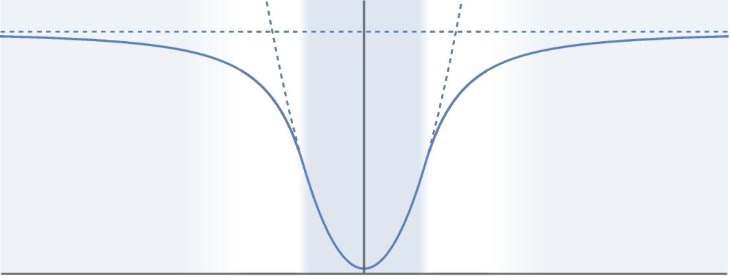
The two regimes cross at |P|=Pc​(α):=2​Meff​(α)/α|P|=P_{\rm c}(\alpha):=\sqrt{2M^{\rm eff}(\alpha)}/\alpha which marks a characteristic momentum scale of the polaron. While the quasi-particle picture is expected to be accurate for |P|≪Pc​(α)|P|\ll P_{\rm c}(\alpha), the radiative regime should hold for |P|≳Pc​(α)|P|\gtrsim P_{\rm c}(\alpha) (see also Remark 1.2 below). Between the two regimes there is no concrete prediction for the behavior of Eα​(P)E_{\alpha}(P). A schematic plot is provided in Figure 1.1.
Refer to caption
Figure 1.1: The energy-momentum relation Eα​(P)E_{\alpha}(P) is expected to have two characteristic regimes: The parabolic quasi-particle regime for small momenta (dark area) and the radiative regime for large momenta (light area). For the transition between the two there is no concrete prediction. The dashed lines denote the quasi-particle energy (1.21) and the bottom of the continuous spectrum (1.23). Their intersection defines the momentum scale Pc​(α)P_{c}(\alpha) that is proportional to α\alpha for large coupling.

One aspect of this work is to show that the quasi-particle picture is mathematically rigorous, insofar as it provides a parabolic upper bound on Eα​(P)E_{\alpha}(P) that coincides with the expected form of the quasi-particle energy in the limit of large coupling. Since the quasi-particle energy (1.21) is determined by the values of Eα​(0)E_{\alpha}(0) and Meff​(α)M^{\rm eff}(\alpha), it is instructive to recall two long-standing open conjectures concerning their behavior for α→∞\alpha\to\infty. As explained in the previous section, the phonon field behaves classically for large coupling, and thus it is expected that Meff​(α)M^{\rm eff}(\alpha) should asymptotically tend to the expression that follows from the corresponding semiclassical counterpart of the problem. This semiclassical theory of the effective mass was introduced by Landau and Pekar in 1948 [29], and, based on this work (see also [50, 14]), it is conjectured that

limα→∞Meff​(α)α4=MLPwithMLP=23​‖∇φ‖L22.\displaystyle\lim_{\alpha\to\infty}\frac{M^{\rm eff}(\alpha)}{\alpha^{4}}\,=\,M^{\rm LP}\quad\text{with}\quad M^{\rm LP}\,=\,\frac{2}{3}|\hskip-1.0pt|\nabla\varphi|\hskip-1.0pt|^{2}_{\text{\tiny{$L^{2}$}}}. (1.24)

Although this problem is many decades old, the best available rigorous result is that Meff​(α)M^{\rm eff}(\alpha) is divergent [36], with a recent proof that it diverges at least as fast as α2/5\alpha^{2/5} [6]. Regarding the ground state energy Eα​(0)E_{\alpha}(0) the prediction from the physics literature (see e.g. [4, 41, 52, 26]) is that

Eα​(0)=ePek+12​α2​TrL2​(HPek−1)+O⁡(α−2−δ)asα→∞E_{\alpha}(0)\,=\,e^{\rm Pek}+\frac{1}{2\alpha^{2}}{\rm Tr}_{L^{2}}(\sqrt{H^{\rm Pek}}-1)+O(\alpha^{-2-\delta})\quad\text{as}\quad\alpha\to\infty (1.25)

for some δ>0\delta>0 (in fact it is predicted that δ=2\delta=2 [26]). Compared to the semiclassical expansion this includes a subleading correction of order α−2\alpha^{-2}, which we call the Bogoliubov energy, and which arises from quantum fluctuations of the field around its classical value. For a nice heuristic derivation of this correction, we recommend the study of [41]. Now inserting (1.24) and (1.25) into (1.21), and based on the expectation that the quasi-particle regime is restricted to |P|≪2​Meff​(α)/α∼α|P|\ll\sqrt{2M^{\rm eff}(\alpha)}/\alpha\sim\alpha, it is clear that the Bogoliubov energy needs to be taken into account in order to see the quasi-particle energy shift given by P2/(2​α4​MLP)≪α−2P^{2}/(2\alpha^{4}M^{\rm LP})\ll\alpha^{-2}. Mathematically, the validity of (1.25) has been established only for confined polaron models [18, 15]. The corresponding upper bound for the unconfined model is a corollary of our main result.

As a summary of the above we arrive at the following claim.

Conjecture.

Let MLPM^{\rm LP} be the Landau–Pekar mass defined in (1.24). There exists a continuous function f:[0,∞)→[0,∞)f:[0,\infty)\rightarrow[0,\infty), satisfying f⁡(s)→1f(s)\to 1 as s→∞s\to\infty and

f⁡(s)\displaystyle f(s) =s2​MLP+O(s2)ass→0,\displaystyle\,=\,\frac{s}{2M^{\rm LP}}+O(s^{2})\quad\text{as}\quad s\to 0, (1.26)

such that for all P∈ℝ3P\in\mathbb{R}^{3}

limα→∞α2​(Eα​(α​P)−ePek−12​α2​TrL2​(HPek−1))=f⁡(P2).\lim_{\alpha\rightarrow\infty}\alpha^{2}\left(E_{\alpha}(\alpha P)-e^{\rm Pek}-\frac{1}{2\alpha^{2}}{\rm Tr}_{L^{2}}\big(\sqrt{H^{\rm Pek}}-1\big)\right)\,=\,f(P^{2}). (1.27)

Our main result, Theorem 2.1 below, provides an upper bound for Eα​(α​P)E_{\alpha}(\alpha P) that is compatible with the conjecture in the quasi-particle regime. To be more precise, our result implies that the left side of (1.27), with the limit replaced by the lim sup\limsup, is bounded from above by P2/(2​MLP)P^{2}/(2M^{\rm LP}) for all P∈ℝ3P\in\mathbb{R}^{3}. This shows that the corrections to the quasi-particle energy are always negative, a conclusion that is not entirely obvious a priori.

Remark 1.1.

An immediate consequence of the conjecture would be that

12​limP→0limα→∞α2​(Eα​(α​P)−Eα​(0)P2)−1=MLP\displaystyle\frac{1}{2}\lim_{P\rightarrow 0}\lim_{\alpha\to\infty}\alpha^{2}\bigg(\frac{E_{\alpha}(\alpha P)-E_{\alpha}(0)}{P^{2}}\bigg)^{-1}\,=\,M^{\rm LP} (1.28)

which is to be compared with (1.24) where the limits are taken in reversed order.

Remark 1.2.

Even though our analysis is focused on the quasi-particle regime, let us mention an interesting problem concerning the radiative regime. The question is whether Eα​(P)E_{\alpha}(P) enters the continuous part of the spectrum, i.e. whether the spectral gap closes at some finite momentum, or not. The answer may in fact depend on the dimension and possibly also on the value of α\alpha. It is known that in two dimensions Eα​(P)E_{\alpha}(P) remains an isolated eigenvalue for all PP, meaning that the curve approaches infσcont​(Hα​(P))\inf\sigma_{\rm cont}(H_{\alpha}(P)) only in the limit |P|→∞|P|\to\infty [51]. To our knowledge in three dimensions the question is not completely settled. While for small momenta it is known that Eα​(P)E_{\alpha}(P) corresponds to a simple eigenvalue [51], there is indication from results obtained for weak coupling that Eα​(P)E_{\alpha}(P) agrees with the bottom of the continuous spectrum when |P||P| is sufficiently large [10].

2 Main Result

We are now ready to state the main result.

Theorem 2.1.

Let Eα​(P)=infσ⁡(Hα​(P))E_{\alpha}(P)=\inf\sigma(H_{\alpha}(P)), MLP=23​‖∇φ‖L22M^{\rm LP}=\frac{2}{3}|\hskip-1.0pt|\nabla\varphi|\hskip-1.0pt|^{2}_{\text{\tiny{$L^{2}$}}} with φ\varphi defined in (1.14) and choose c>0c>0. For every ε>0\varepsilon>0 there exists a constant Cc,ε>0C_{c,\varepsilon}>0 such that

Eα​(P)≤ePek+TrL2​(HPek−1)2​α2+P22​α4​MLP+Cc,ε​α−52+ε\displaystyle E_{\alpha}(P)\,\leq\,e^{\rm Pek}+\frac{{\rm Tr}_{L^{2}}(\sqrt{H^{\rm Pek}}-1)}{2\alpha^{2}}+\frac{P^{2}}{2\alpha^{4}M^{\rm LP}}+C_{c,\varepsilon}\,\alpha^{-\frac{5}{2}+\varepsilon} (2.1)

for all |P|/α≤c|P|/\alpha\leq c and all α\alpha large enough.

Since the operator HPek−1\sqrt{H^{\rm Pek}}-1 is trace class, non-zero and non-positive (see Lemma 1.1), the second term on the right side is finite and lowers the energy. It corresponds to the predicted quantum corrections of the ground state energy of the Fröhlich Hamiltonian [4, 41, 52, 26]. Since Eα​(0)=infσ⁡(Hα)E_{\alpha}(0)=\inf\sigma(H_{\alpha}), our theorem implies a two-term upper bound for the ground state energy of the Fröhlich Hamiltonian that agrees with this prediction. For momenta in the range α−14+ε2≪|P|/α≤c\alpha^{-\frac{1}{4}+\frac{\varepsilon}{2}}\ll|P|/\alpha\leq c, the last term in (2.1) is subleading for large α\alpha when compared to the momentum dependent term. In this region the upper bound describes a quadratic dispersion relation for a free quasi-particle with mass α4​MLP\alpha^{4}M^{\rm LP}. The upper restriction on the range of |P||P| is natural, since for |P|/α≥2​MLP|P|/\alpha\geq\sqrt{2M^{\rm LP}} the right side of (2.1) would be larger than the value of the bottom of the continuous spectrum (1.23). The lower restriction |P|/α≫α−14+ε2|P|/\alpha\gg\alpha^{-\frac{1}{4}+\frac{\varepsilon}{2}}, on the other hand, could in principle be improved by deriving a better error term in (2.1).

The derivation of a matching lower bound is, of course, more involved. To our knowledge the best known parabolic lower bound is still the one obtained by Lieb and Yamazaki [38] in 1958 stating that Eα​(P)≥c1​ePek+c2​P2/(2​α4​MLP)E_{\alpha}(P)\geq c_{1}e^{\rm Pek}+c_{2}P^{2}/(2\alpha^{4}M^{\rm LP}) with c1≈3.07c_{1}\approx 3.07 and c2≈0.11c_{2}\approx 0.11. Even for P=0P=0 it remains a challenging problem to improve the Lieb–Thomas bound (1.15) such that it includes the quantum corrections of order α−2\alpha^{-2}. Progress in this direction has been achieved in [18, 15] for simplified polaron models in which the electron and the quantum field are confined to suitable finite size regions.

In the next two sections we provide the definition of our trial state and formulate our main statement as a variational estimate. The remainder of the paper is devoted to the proof of the variational estimate. A sketch of the strategy of the proof is given in Section 3.2.

2.1 Bogoliubov Hamiltonian

In this section we introduce and discuss a quadratic Hamiltonian defined on the Fock space. For its definition we set Π0\Pi_{0} and Π1\Pi_{1} to be the orthogonal projectors onto KerHPek=Span{∂iφ:i=1,2,3}\textnormal{Ker}H^{\rm Pek}=\text{Span}\{\partial_{i}\varphi:i=1,2,3\} and (Ker​HPek)⟂(\textnormal{Ker}H^{\rm Pek})^{\perp}, that is

Ran​(Π0)=Ker​HPek,Ran​(Π1)=(Ker​HPek)⟂.\displaystyle\text{Ran}(\Pi_{0})\,=\,\text{Ker}H^{\rm Pek},\quad\text{Ran}(\Pi_{1})\,=\,(\text{Ker}H^{\rm Pek})^{\perp}. (2.2)

Even though we will not make explicit use of it, it is convenient to keep in mind that the decomposition L2​(ℝ3)=Ran​(Π0)⊕Ran​(Π1)L^{2}(\mathbb{R}^{3})\,=\,\text{Ran}(\Pi_{0})\oplus\text{Ran}(\Pi_{1}) implies the factorization

ℱ=ℱ0⊗ℱ1withℱ0=ℱ⁡(Ran​(Π0))andℱ1=ℱ⁡(Ran​(Π1)).\displaystyle\mathcal{F}=\mathcal{F}_{0}\otimes\mathcal{F}_{1}\quad\textnormal{with}\quad\mathcal{F}_{0}=\mathcal{F}(\text{Ran}(\Pi_{0}))\quad\textnormal{and}\quad\mathcal{F}_{1}=\mathcal{F}(\text{Ran}(\Pi_{1})). (2.3)

For technical reasons, which are explained in Section 3.4.3, we introduce the Bogoliubov Hamiltonian ℍK\mathbb{H}_{K} with a momentum cutoff K∈(0,∞]K\in(0,\infty]. Setting ℕ1=d​Γ​(Π1)\mathbb{N}_{1}=\textnormal{d}\Gamma(\Pi_{1}) (the number operator on ℱ1\mathcal{F}_{1}) we define

ℍK=ℕ1−⟨ψ|ϕ⁡(hK,⋅1)​R​ϕ​(hK,⋅1)​ψ⟩L2,\displaystyle\mathbb{H}_{K}\,=\,\mathbb{N}_{1}-\big\langle\psi\big|\phi(h_{K,\cdot}^{1})R\phi(h_{K,\cdot}^{1})\psi\big\rangle_{\text{\tiny{$L^{2}$}}}, (2.4)

where the new coupling function

hK,x1​(y)=∫d​z​Π1​(y,z)​hK,x​(z)withhK,x​(y)=1(2​π)3​∫|k|≤Kei​k​(x−y)|k|​d​k\displaystyle h_{K,x}^{1}(y)\,=\,\int\textnormal{d}z\,\Pi_{1}(y,z)h_{K,x}(z)\quad\text{with}\quad h_{K,x}(y)\,=\,\frac{1}{(2\pi)^{3}}\int_{|k|\leq K}\frac{e^{ik(x-y)}}{|k|}\textnormal{d}k (2.5)

results from the coupling function hxh_{x} by removing all momenta larger than KK and then projecting to Ran​(Π1)\text{Ran}(\Pi_{1}). The second term in (2.4) defines the quadratic operator given by

⟨ψ|ϕ⁡(hK,⋅1)​R​ϕ​(hK,⋅1)​ψ⟩L2\displaystyle\big\langle\psi\big|\phi(h^{1}_{K,\cdot})R\phi(h^{1}_{K,\cdot})\psi\big\rangle_{\text{\tiny{$L^{2}$}}}
=∬d​y​d​z​⟨ψ|(hK,⋅1)​(y)​R​(hK,⋅1)​(z)​ψ⟩L2​(ay†+ay)​(az†+az).\displaystyle\quad\quad=\iint\textnormal{d}y\textnormal{d}z\,\big\langle\psi\big|(h^{1}_{K,\cdot})(y)R(h^{1}_{K,\cdot})(z)\psi\big\rangle_{\text{\tiny{$L^{2}$}}}(a_{y}^{\dagger}+a_{y})(a_{z}^{\dagger}+a_{z}). (2.6)

By definition ℍK\mathbb{H}_{K} acts non-trivially only on the tensor component ℱ1\mathcal{F}_{1}. Below we will show that ℍK\mathbb{H}_{K} is bounded from below and diagonalizable by a unitary Bogoliubov transformation. For the precise statement, we need some further preparations.

For K∈(0,∞]K\in(0,\infty] we introduce HKPekH^{\rm Pek}_{K} as the operator on L2​(ℝ3)L^{2}(\mathbb{R}^{3}) defined by

HKPek↾Ran​(Π1)\displaystyle H^{\rm Pek}_{K}\restriction\textnormal{Ran}(\Pi_{1}) =Π1−4​TK\displaystyle\,=\,\Pi_{1}-4T_{K} (2.7a)
HKPek↾Ran​(Π0)\displaystyle H^{\rm Pek}_{K}\restriction\textnormal{Ran}(\Pi_{0}) = 0\displaystyle\,=\,0 (2.7b)

where TKT_{K} is defined by the integral kernel

TK​(y,z)\displaystyle T_{K}(y,z) =Re⁡⟨ψ|hK,⋅1​(y)​R​hK,⋅1​(z)​ψ⟩L2.\displaystyle\,=\,\operatorname{Re}\big\langle\psi\big|h^{1}_{K,\cdot}(y)Rh^{1}_{K,\cdot}(z)\psi\big\rangle_{\text{\tiny{$L^{2}$}}}. (2.8)

By definition H∞Pek=HPekH^{\rm Pek}_{\infty}=H^{\rm Pek}, see (1.20). Moreover we set ΘK=(HKPek)1/4\Theta_{K}=(H^{\rm Pek}_{K})^{1/4} and

AK↾Ran​(Π1)\displaystyle A_{K}\restriction\text{Ran}(\Pi_{1}) =ΘK−1+ΘK2\displaystyle\,=\,\frac{\Theta_{K}^{-1}+\Theta_{K}}{2} BK↾Ran​(Π1)=ΘK−1−ΘK2\displaystyle\hskip-56.9055ptB_{K}\restriction\text{Ran}(\Pi_{1})\,=\,\frac{\Theta_{K}^{-1}-\Theta_{K}}{2} (2.9a)
AK↾Ran​(Π0)\displaystyle A_{K}\restriction\text{Ran}(\Pi_{0}) =Π0\displaystyle\,=\,\Pi_{0} BK↾Ran​(Π0)= 0.\displaystyle\hskip-56.9055ptB_{K}\restriction\text{Ran}(\Pi_{0})\,=\,0. (2.9b)

The next lemma, whose proof can be found in Section 4, implies some useful properties of these operators, among others, that there is a constant C>0C>0 such that

supK≥K0(‖AK‖op+‖BK‖HS)≤C\displaystyle\sup_{K\geq K_{0}}\big(|\hskip-1.0pt|A_{K}|\hskip-1.0pt|_{\text{\tiny{$\rm op$}}}+|\hskip-1.0pt|B_{K}|\hskip-1.0pt|_{\text{\tiny{$\rm HS$}}}\big)\leq C (2.10)

for some K0K_{0} large enough.

Lemma 2.2.

For K0K_{0} large enough there exist constants β∈(0,1)\beta\in(0,1) and C>0C>0 such that

  • (i)

    0≤HKPek≤10\leq H^{\rm Pek}_{K}\leq 1 and (HKPek−β)↾Ran​(Π1)≥0(H^{\rm Pek}_{K}-\beta)\restriction\textnormal{Ran}(\Pi_{1})\geq 0

  • (ii)

    (BK)2≤C⁡(1−HKPek)(B_{K})^{2}\leq C(1-H_{K}^{\rm Pek})

  • (iii)

    TrL2​(1−HKPek)≤C{\rm{Tr}}_{L^{2}}(1-H_{K}^{\rm Pek})\leq C

for all K∈(K0,∞]K\in(K_{0},\infty]. Moreover for all K∈(K0,∞)K\in(K_{0},\infty)

  • (iv)

    TrL2((−i∇)(1−HKPek)(−i∇))≤CK{\rm{Tr}}_{L^{2}}((-i\nabla)(1-H_{K}^{\rm Pek})(-i\nabla))\leq CK.

Up to normal ordering the Hamiltonian ℍK\mathbb{H}_{K} corresponds to the second quantization of HKPekH^{\rm Pek}_{K}. From the properties of the latter we can deduce that ℍK\mathbb{H}_{K} is diagonizable by a unitary Bogoliubov transformation. To this end we introduce the transformation

𝕌K.a(f)𝕌K†\displaystyle\mathbb{U}^{{\color[rgb]{1,1,1}.}}_{K}a(f)\mathbb{U}^{\dagger}_{K}\, =a⁡(AK​f)+a†​(BK​f¯)for all​f∈L2​(ℝ3).\displaystyle=\,a(A_{K}f)+a^{\dagger}(B_{K}\overline{f})\quad\text{for all}\ f\in L^{2}(\mathbb{R}^{3}). (2.11)

That this transformation defines a unitary operator 𝕌K\mathbb{U}_{K} for all K∈(K0,∞]K\in(K_{0},\infty] is a consequence of (2.10). This is known as the Shale-Stinespring condition and we refer to [49] for more details. Also note that 𝕌K\mathbb{U}_{K} does not mix the two components in ℱ=ℱ0⊗ℱ1\mathcal{F}=\mathcal{F}_{0}\otimes\mathcal{F}_{1}.

Lemma 2.3.

For K∈(K0,∞]K\in(K_{0},\infty] with K0K_{0} large enough and 𝕌K\mathbb{U}_{K} the unitary operator defined by (2.11), we have

𝕌.Kℍ.K𝕌†K\displaystyle\mathbb{U}^{{\color[rgb]{1,1,1}.}}_{K}\mathbb{H}^{{\color[rgb]{1,1,1}.}}_{K}\mathbb{U}^{\dagger}_{K} =d​Γ​(HKPek)+12​TrL2​(HKPek−Π1)\displaystyle\,=\,\textnormal{d}\Gamma(\sqrt{H^{\rm Pek}_{K}})+\frac{1}{2}\textnormal{Tr}_{L^{2}}(\sqrt{H^{\rm Pek}_{K}}-\Pi_{1}) (2.12)

with HKPekH^{\rm Pek}_{K} defined by (2.7a) and (2.7b).

The proof is obtained by an explicit computation and postponed to Section 4. From this lemma, we can infer that the ground state energy of ℍK\mathbb{H}_{K} is given by

infσ⁡(ℍK)=12​TrL2​(HKPek−Π1)=12​TrL2​(HKPek−1)+32,\displaystyle\inf\sigma(\mathbb{H}_{K})\,=\,\frac{1}{2}\textnormal{Tr}_{L^{2}}\big(\sqrt{H^{\rm Pek}_{K}}-\Pi_{1}\big)\,=\,\frac{1}{2}\textnormal{Tr}_{L^{2}}\big(\sqrt{H^{\rm Pek}_{K}}-1\big)+\frac{3}{2}, (2.13)

where we also used Π1=1−Π0\Pi_{1}=1-\Pi_{0} and TrL2​(Π0)=3\text{Tr}_{L^{2}}(\Pi_{0})=3. Moreover, since HKPek≤Π1H^{\rm Pek}_{K}\leq\Pi_{1} we have infσ⁡(ℍK)<0\inf\sigma(\mathbb{H}_{K})<0 and from Item (iv) of Lemma 2.2 we find that infσ⁡(ℍK)>−∞\inf\sigma(\mathbb{H}_{K})>-\infty uniformly in K→∞K\to\infty.

For the ground state of ℍ.K\mathbb{H}^{{\color[rgb]{1,1,1}.}}_{K} we shall use the notation

ΥK=𝕌K†​Ω,\displaystyle\Upsilon_{K}\,=\,\mathbb{U}_{K}^{\dagger}\Omega, (2.14)

where it is important to keep in mind that the state ΥK\Upsilon_{K} has excitations only in ℱ1\mathcal{F}_{1} (i.e., no zero-mode excitations) since 𝕌K†\mathbb{U}_{K}^{\dagger} acts as the identity on ℱ0\mathcal{F}_{0}, see (2.9b).

2.2 Trial state and variational estimate

As starting point for the definition of our trial state consider the Fock space wave function obtained from the fiber decomposition of the classical Pekar product state Ψψ,φ\Psi_{\psi,\varphi}, that is

ΨαPek​(P)\displaystyle\Psi^{\rm Pek}_{\alpha}(P) =∫d​x​ei⁡(Pf−P)​x​ψ​(x)​ea†​(α​φ)​Ω.\displaystyle\,=\,\int\textnormal{d}x\,e^{i(P_{f}-P)x}\psi(x)e^{a^{\dagger}(\alpha\varphi)}\Omega. (2.15)

Testing the energy of Hα​(P)H_{\alpha}(P) with ΨαPek​(P)\Psi^{\rm Pek}_{\alpha}(P), one would in fact obtain that Eα​(P)E_{\alpha}(P) is bounded from above by

ePek−32​α2+P2α4​MLP+o⁡(α−2).\displaystyle e^{\rm Pek}-\frac{3}{2\alpha^{2}}+\frac{P^{2}}{\alpha^{4}M^{\rm LP}}+o(\alpha^{-2}). (2.16)

For Eα​(0)E_{\alpha}(0) this provides already a better bound compared to the semiclassical approximation for infσ⁡(Hα)\inf\sigma(H_{\alpha}). The improvement comes from taking into account the translational symmetry and can be interpreted as the missing zero-point energy of three quantum oscillators (that turned into translational degrees of freedom). As a side remark, we find it somewhat surprising that fiber decompositions of this form have been employed very rarely in the polaron literature, exceptions being [27] and [46]. We think they could be of interest also for other translation-invariant polaron type models.

To obtain the desired bound for Eα​(P)E_{\alpha}(P), we need to add several modifications to the integrand in (2.15). On the one hand, we have to replace the classical field φ\varphi by a suitably shifted φP\varphi_{P} in order to get the correct momentum dependent term (note that (2.16) is missing a factor 12\frac{1}{2} in the quadratic term). The missing part of the rest energy (compare with (2.13)), on the other hand, is caused by two types of correlations that need to be added to the Pekar product state. First, we include correlations between the electron and the phonons. This is done in the spirit of first-order adiabatic perturbation theory. Second, we rotate the vacuum by the unitary transformation (2.11) that diagonalizes the Bogoliubov Hamiltonian (2.4). As discussed, the latter describes the quantum fluctuations of the phonons around the classical field. For technical reasons, briefly explained in Section 3.2, we also need to introduce suitable momentum and space cutoffs in the trial state.

Explicitly, we consider the family of Fock space wave functions ΨK,α​(P)∈ℱ\Psi_{K,\alpha}(P)\in\mathcal{F}, depending on the coupling α\alpha, the total momentum P∈ℝ3P\in\mathbb{R}^{3} and the cutoff K∈(K0,∞)K\in(K_{0},\infty), given by

ΨK,α​(P)\displaystyle\Psi_{K,\alpha}(P) =∫d​x​ei⁡(Pf−P)​x​ea†​(α​φP)−a⁡(α​φP)​(GK,x0−α−1​GK,x1)\displaystyle\,=\,\int\textnormal{d}x\,e^{i(P_{f}-P)x}\,e^{a^{\dagger}(\alpha\varphi_{P})-a(\alpha\varphi_{P})}\big(G^{0}_{K,x}-\alpha^{-1}G^{1}_{K,x}\big) (2.17)

where

φP=φ+iξPwithξP=1α2​MLP(P∇)φ,MLP=23||∇φ||L22,\displaystyle\varphi_{P}\,=\,\varphi+i\xi_{P}\quad\text{with}\quad\xi_{P}\,=\,\frac{1}{\alpha^{2}M^{\rm LP}}(P\nabla)\varphi,\quad M^{\rm LP}=\frac{2}{3}|\hskip-1.0pt|\nabla\varphi|\hskip-1.0pt|^{2}_{\text{\tiny{$L^{2}$}}}, (2.18)

and

GK,x0\displaystyle G^{0}_{K,x} =ψ(x)ΥK,GK,x1=uα(x)(Rϕ(hK,⋅1)ψ)(x)ΥKandΥK=𝕌K†Ω.\displaystyle\,=\,\psi(x)\Upsilon_{K},\quad G^{1}_{K,x}=u_{\alpha}(x)(R\phi(h^{1}_{K,\cdot})\psi)(x)\Upsilon_{K}\quad\text{and}\quad\Upsilon_{K}=\mathbb{U}_{K}^{\dagger}\Omega. (2.19)

Here uα:ℝ3→[0,1]u_{\alpha}:\mathbb{R}^{3}\to[0,1] is a radial function, satisfying

uα​(x)={1∀|x|≤α0∀|x|≥2​αand‖∇uα‖L∞+‖Δ​uα‖L∞≤C​α−1\displaystyle u_{\alpha}(x)\,=\,\begin{cases}1&\forall\ |x|\leq\alpha\\ 0&\forall\ |x|\geq 2\alpha\end{cases}\quad\quad\text{and}\quad\quad|\hskip-1.0pt|\nabla u_{\alpha}|\hskip-1.0pt|_{\text{\tiny{$L^{\infty}$}}}+|\hskip-1.0pt|\Delta u_{\alpha}|\hskip-1.0pt|_{\text{\tiny{$L^{\infty}$}}}\,\leq\,C\alpha^{-1} (2.20)

for some C>0C>0. For completeness, we recall that ψ>0\psi>0 and φ\varphi are the unique rotational invariant minimizers of the Pekar functionals (1.12) and (1.13).

Remark 2.1.

Writing GK,xiG_{K,x}^{i} we think of these states as elements in L2​(ℝ3,ℱ)L^{2}(\mathbb{R}^{3},\mathcal{F}) and of

(R​ϕ​(hK,⋅1)​ψ)​(x)=∬d​z​d​y​R​(x,y)​hK,y1​(z)​ψ​(y)​(az†+az)\displaystyle(R\phi(h^{1}_{K,\cdot})\psi)(x)\,=\,\iint\textnormal{d}z\textnormal{d}y\,R(x,y)h_{K,y}^{1}(z)\psi(y)\,\big(a^{\dagger}_{z}+a_{z}\big) (2.21)

as an xx-dependent Fock space operator. Via the isomorphism L2​(ℝ3,ℱ)≃ℋL^{2}(\mathbb{R}^{3},\mathcal{F})\simeq\mathscr{H}, we can view GK,xiG_{K,x}^{i} also as a wave function in ℋ\mathscr{H}. In this case we shall write

GK0=ψ⊗ΥK,GK1=uα​R​ϕ​(hK,⋅1)​ψ⊗ΥK.\displaystyle G^{0}_{K}\,=\,\psi\otimes\Upsilon_{K},\quad G_{K}^{1}\,=\,u_{\alpha}R\phi(h^{1}_{K,\cdot})\psi\otimes\Upsilon_{K}. (2.22)

For the introduced trial states, we prove the following variational estimate, where ℍ∞\mathbb{H}_{\infty} denotes the Bogoliubov Hamiltonian (2.4) for K=∞K=\infty.

Proposition 2.4.

Let ΨK,α​(P)∈ℱ\Psi_{K,\alpha}(P)\in\mathcal{F} as in (2.17), choose c,c~>0c,\tilde{c}>0 and set r(K,α)=K−1/2α−2+Kα−3r(K,\alpha)=K^{-1/2}\alpha^{-2}+\sqrt{K}\alpha^{-3}. For every ε>0\varepsilon>0 there exists a constant Cε>0C_{\varepsilon}>0 (we omit the dependence on cc and c~\tilde{c}) such that

⟨ΨK,α​(P)|Hα​(P)​ΨK,α​(P)⟩ℱ⟨ΨK,α​(P)|ΨK,α​(P)⟩ℱ≤ePek+infσ⁡(ℍ∞)−32α2+P22​α4​MLP+Cε​αε​r​(K,α)\displaystyle\frac{\big\langle\Psi_{K,\alpha}(P)|H_{\alpha}(P)\Psi_{K,\alpha}(P)\big\rangle_{\text{\tiny{$\mathcal{F}$}}}}{\big\langle\Psi_{K,\alpha}(P)|\Psi_{K,\alpha}(P)\big\rangle_{\text{\tiny{$\mathcal{F}$}}}}\,\leq\,e^{\rm Pek}+\frac{\inf\sigma(\mathbb{H}_{\infty})-\frac{3}{2}}{\alpha^{2}}+\frac{P^{2}}{2\alpha^{4}M^{\rm LP}}+C_{\varepsilon}\alpha^{\varepsilon}r(K,\alpha) (2.23)

for all |P|/α≤c|P|/\alpha\leq c and all KK, α\alpha large enough with K/α≤c~K/\alpha\leq\tilde{c}.

With (2.13) and H∞Pek=HPekH_{\infty}^{\rm Pek}=H^{\rm Pek} we can rewrite the term of order α−2\alpha^{-2} as

infσ⁡(ℍ∞)−32=12​TrL2​(HPek−1).\displaystyle\inf\sigma(\mathbb{H}_{\infty})-\frac{3}{2}\,=\,\frac{1}{2}\textnormal{Tr}_{L^{2}}\big(\sqrt{H^{\rm Pek}}-1\big). (2.24)

Choosing KK now proportional to α\alpha optimizes the asymptotics of the error in (2.23) and proves Theorem 2.1.

3 Proof of Proposition 2.4

We recall the definition of the field operators

ϕ⁡(f)=a†​(f)+a⁡(f),π⁡(f)=ϕ⁡(i​f)\displaystyle\phi(f)=a^{\dagger}(f)+a(f),\quad\pi(f)=\phi(if) (3.1)

and the Weyl operator

W⁡(f)=e−i​π​(f)=ea†​(f)−a​(f)=ea†​(f)​e−a⁡(f)​e−12​‖f‖L22.\displaystyle W(f)\,=\,e^{-i\pi(f)}\,=\,e^{a^{\dagger}(f)-a(f)}\,=\,e^{a^{\dagger}(f)}e^{-a(f)}e^{-\frac{1}{2}|\hskip-1.0pt|f|\hskip-1.0pt|^{2}_{\text{\tiny{$L^{2}$}}}}. (3.2)

The Weyl operator is unitary and satisfies

W†​(f)=W⁡(−f),W⁡(f)​W​(g)=W⁡(g)​W​(f)​e2​i​Im⁡⟨g|f⟩L2=W⁡(f+g)​ei​Im⁡⟨g|f⟩L2.\displaystyle W^{\dagger}(f)\,=\,W(-f),\quad W(f)W(g)\,=\,W(g)W(f)e^{2i\operatorname{Im}\langle g|f\rangle_{\text{\tiny{$L^{2}$}}}}\,=\,W(f+g)e^{i\operatorname{Im}\langle g|f\rangle_{\text{\tiny{$L^{2}$}}}}. (3.3)

3.1 The total energy

The proof of Proposition 2.4 starts with a convenient formula for the energy evaluated in the trial state. For the precise statement, we introduce the yy-dependent function in L2​(ℝ3)L^{2}(\mathbb{R}^{3}),

wP,y=(1−e−y∇)φP,\displaystyle w_{P,y}\,=\,(1-e^{-y\nabla})\varphi_{P}, (3.4)

and the yy-dependent Fock space operator

AP,y=iPfy+igP(y),gP(y)=−2MLP∫01ds⟨φ|e−sy∇(y∇)3(P∇)φ⟩L2.\displaystyle A_{P,y}\,=\,iP_{f}y+ig_{P}(y),\quad g_{P}(y)\,=\,-\frac{2}{M^{\rm LP}}\int_{0}^{1}\textnormal{d}s\,\langle\varphi|e^{-sy\nabla}(y\nabla)^{3}(P\nabla)\varphi\rangle_{\text{\tiny{$L^{2}$}}}. (3.5)

Since gP​(y)g_{P}(y) is real-valued we have (AP,y)†=−AP,y(A_{P,y})^{\dagger}=-A_{P,y}. We further consider the Weyl-transformed Fröhlich Hamiltonian,

H~α,P=W​(α​φP)†​(Hα−ePek)​W​(α​φP)\displaystyle\widetilde{H}_{\alpha,P}\,=\,W(\alpha\varphi_{P})^{\dagger}\big(H_{\alpha}-e^{\rm Pek}\big)W(\alpha\varphi_{P})\, =hPek+α−2​ℕ+α−1​ϕ​(hx+φP),\displaystyle=\,h^{\rm Pek}+\alpha^{-2}\mathbb{N}+\alpha^{-1}\phi(h_{x}+\varphi_{P}), (3.6)

where we recall hPek=−Δ+Vφ−λPekh^{\rm Pek}=-\Delta+V^{\varphi}-\lambda^{\rm Pek}, and denote the shift operator acting on L2​(ℝ3)L^{2}(\mathbb{R}^{3}) by Ty=ey∇T_{y}=e^{y\nabla} with y∈ℝ3y\in\mathbb{R}^{3}.

Lemma 3.1.

For ΨK,α​(P)\Psi_{K,\alpha}(P) defined in (2.17) we have

⟨ΨK,α​(P)|Hα​(P)​ΨK,α​(P)⟩ℱ\displaystyle\big\langle\Psi_{K,\alpha}(P)|H_{\alpha}(P)\Psi_{K,\alpha}(P)\big\rangle_{\text{\tiny{$\mathcal{F}$}}} =(ePek+P22​α4​MLP)​𝒩+ℰ+𝒢+𝒦\displaystyle\,=\,\Big(e^{\rm Pek}+\frac{P^{2}}{2\alpha^{4}M^{\rm LP}}\Big)\,\mathcal{N}+\mathcal{E}+\mathcal{G}+\mathcal{K} (3.7)

where 𝒩=‖ΨK,α​(P)‖ℱ2\mathcal{N}=|\hskip-1.0pt|\Psi_{K,\alpha}(P)|\hskip-1.0pt|^{2}_{\text{\tiny{$\mathcal{F}$}}} and

ℰ\displaystyle\mathcal{E} =∫d​y​⟨GK0|H~α,P​Ty​eAP,y​W​(α​wP,y)​GK0⟩ℋ\displaystyle\,=\,\int\textnormal{d}y\,\big\langle G_{K}^{0}|\widetilde{H}_{\alpha,P}T_{y}e^{A_{P,y}}W(\alpha w_{P,y})G_{K}^{0}\big\rangle_{\text{\tiny{$\mathscr{H}$}}} (3.8a)
𝒢\displaystyle\mathcal{G} =−2α∫dyRe⟨GK0|H~α,PTyeAP,yW(αwP,y)GK1⟩ℋ\displaystyle\,=\,-\frac{2}{\alpha}\int\textnormal{d}y\,\operatorname{Re}\big\langle G_{K}^{0}|\widetilde{H}_{\alpha,P}T_{y}e^{A_{P,y}}W(\alpha w_{P,y})G_{K}^{1}\big\rangle_{\text{\tiny{$\mathscr{H}$}}} (3.8b)
𝒦\displaystyle\mathcal{K} =1α2​∫d​y​⟨GK1|H~α,P​Ty​eAP,y​W​(α​wP,y)​GK1⟩ℋ.\displaystyle\,=\,\frac{1}{\alpha^{2}}\int\textnormal{d}y\,\big\langle G_{K}^{1}|\widetilde{H}_{\alpha,P}T_{y}e^{A_{P,y}}W(\alpha w_{P,y})G_{K}^{1}\big\rangle_{\text{\tiny{$\mathscr{H}$}}}. (3.8c)

For the proof we recall that the Weyl operator shifts the creation and annihilation operators by complex numbers,

W​(g)†​a†​(f)​W​(g)=a†​(f)+⟨g|f⟩L2,W​(g)†​a​(f)​W​(g)=a⁡(f)+⟨g|f⟩L2¯,\displaystyle W(g)^{\dagger}a^{\dagger}(f)W(g)\,=\,a^{\dagger}(f)+\langle g|f\rangle_{\text{\tiny{$L^{2}$}}},\quad W(g)^{\dagger}a(f)W(g)\,=\,a(f)+\overline{\langle g|f\rangle_{\text{\tiny{$L^{2}$}}}}, (3.9)

and, as a simple consequence,

W​(g)†​ϕ​(f)​W​(g)\displaystyle W(g)^{\dagger}\phi(f)W(g) =ϕ⁡(f)+2​Re⁡⟨f|g⟩L2,\displaystyle\,=\,\phi(f)+2\operatorname{Re}\big\langle f|g\big\rangle_{\text{\tiny{$L^{2}$}}}, (3.10a)
W​(g)†​ℕ​W​(g)\displaystyle W(g)^{\dagger}\mathbb{N}W(g) =ℕ+ϕ⁡(g)+‖g‖L22,\displaystyle\,=\,\mathbb{N}+\phi(g)+|\hskip-1.0pt|g|\hskip-1.0pt|^{2}_{\text{\tiny{$L^{2}$}}}, (3.10b)
W​(g)†​Pf​W​(g)\displaystyle W(g)^{\dagger}P_{f}W(g) =Pf−a†(i∇g)−a(i∇g)−⟨g|i∇g⟩L2.\displaystyle\,=\,P_{f}-a^{\dagger}(i\nabla g)-a(i\nabla g)-\big\langle g|i\nabla g\big\rangle_{\text{\tiny{$L^{2}$}}}. (3.10c)

Moreover we need the following identity.

Lemma 3.2.

Let φP=φ+i​ξP\varphi_{P}=\varphi+i\xi_{P} with ξP\xi_{P} defined by (2.18). Then

W†​(α​φP)​ei⁡(Pf−P)​y​W​(α​φP)\displaystyle W^{\dagger}(\alpha\varphi_{P})e^{i(P_{f}-P)y}W(\alpha\varphi_{P}) =eAP,y​W​(α​wP,y).\displaystyle\,=\,e^{A_{P,y}}W(\alpha w_{P,y}). (3.11)
Proof of Lemma 3.2.

We first observe that

e−i​Pf​y​a†​(f)​ei​Pf​y\displaystyle e^{-iP_{f}y}a^{\dagger}(f)e^{iP_{f}y} =a†(e−y∇f)\displaystyle\,=\,a^{\dagger}(e^{-y\nabla}f) (3.12)

which follows from dd​se−i​s​Pf​ya†(e(s−1)y∇f)ei​s​Pf​y=0\frac{d}{ds}e^{-isP_{f}y}a^{\dagger}(e^{(s-1)y\nabla}f)e^{isP_{f}y}=0. In combination with (3.3) this leads to

W†​(α​φP)​ei​Pf​y​W​(α​φP)\displaystyle W^{\dagger}(\alpha\varphi_{P})e^{iP_{f}y}W(\alpha\varphi_{P}) =ei​Pf​yW(α(1−e−y∇)φP)exp(iα2Im⟨φP|e−y∇φP⟩L2).\displaystyle\,=\,e^{iP_{f}y}W(\alpha(1-e^{-y\nabla})\varphi_{P})\exp\big(i\alpha^{2}\operatorname{Im}\langle\varphi_{P}|e^{-y\nabla}\varphi_{P}\rangle_{\text{\tiny{$L^{2}$}}}\big). (3.13)

Recalling φP=φ+i1α2​MLP(P∇)φ\varphi_{P}=\varphi+i\frac{1}{\alpha^{2}M^{\rm LP}}(P\nabla)\varphi, we compute

α2​Im\displaystyle\alpha^{2}\operatorname{Im} ⟨φP|e−y∇φP⟩L2=2MLP⟨φ|e−y∇(P∇)φ⟩L2\displaystyle\langle\varphi_{P}|e^{-y\nabla}\varphi_{P}\rangle_{\text{\tiny{$L^{2}$}}}\,=\,\frac{2}{M^{\rm LP}}\langle\varphi|e^{-y\nabla}(P\nabla)\varphi\rangle_{\text{\tiny{$L^{2}$}}}
=−2MLP⟨φ|(y∇)(P∇)φ⟩L2−2MLP∫01ds⟨φ|e−sy∇(y∇)3(P∇)φ⟩L2\displaystyle=\,-\frac{2}{M^{\rm LP}}\langle\varphi|(y\nabla)(P\nabla)\varphi\rangle_{\text{\tiny{$L^{2}$}}}-\frac{2}{M^{\rm LP}}\int_{0}^{1}\textnormal{d}s\,\langle\varphi|e^{-sy\nabla}(y\nabla)^{3}(P\nabla)\varphi\rangle_{\text{\tiny{$L^{2}$}}} (3.14)

where we inserted e−y∇=1−(y∇)+12(y∇)2−∫01dse−sy∇(y∇)3e^{-y\nabla}=1-(y\nabla)+\frac{1}{2}(y\nabla)^{2}-\int_{0}^{1}\textnormal{d}s\,e^{-sy\nabla}(y\nabla)^{3} and used that, due to rotational invariance of φ\varphi, ⟨φ|(P∇)φ⟩L2=0=⟨φ|(y∇)2(P∇)φ⟩L2\langle\varphi|(P\nabla)\varphi\rangle_{\text{\tiny{$L^{2}$}}}=0=\langle\varphi|(y\nabla)^{2}(P\nabla)\varphi\rangle_{\text{\tiny{$L^{2}$}}}. Also because of rotational invariance,

⟨φ|(y∇)(P∇)φ⟩L2=−(P​y)3||∇φ||L22=−(P​y)2MLP,\displaystyle\langle\varphi|(y\nabla)(P\nabla)\varphi\rangle_{\text{\tiny{$L^{2}$}}}\,=\,-\frac{(Py)}{3}|\hskip-1.0pt|\nabla\varphi|\hskip-1.0pt|_{\text{\tiny{$L^{2}$}}}^{2}\,=\,-\frac{(Py)}{2}M^{\rm LP}, (3.15)

and thus, α2Im⟨φP|e−y∇φP⟩L2=Py+gP(y)\alpha^{2}\operatorname{Im}\langle\varphi_{P}|e^{-y\nabla}\varphi_{P}\rangle_{\text{\tiny{$L^{2}$}}}=Py+g_{P}(y). ∎

Proof of Lemma 3.1.

The norm squared is given by

𝒩\displaystyle\mathcal{N} =‖∫d​x​ei⁡(Pf−P)​x​W​(α​φP)​(GK,x0−α−1​GK,x1)‖ℱ2\displaystyle=\Big\|\int\textnormal{d}x\,e^{i(P_{f}-P)x}W(\alpha\varphi_{P})\big(G^{0}_{K,x}-\alpha^{-1}G^{1}_{K,x}\big)\Big\|^{2}_{\text{\tiny{$\mathcal{F}$}}}
=∑i∈{0,1}α−2​i​∬d​y​d​x​⟨GK,xi|W​(α​φP)†​ei⁡(Pf−P)​(y−x)​W​(α​φP)​GK,yi⟩ℱ\displaystyle=\sum_{i\in\{0,1\}}\alpha^{-2i}\iint\textnormal{d}y\textnormal{d}x\,\big\langle G_{K,x}^{i}|W(\alpha\varphi_{P})^{\dagger}e^{i(P_{f}-P)(y-x)}W(\alpha\varphi_{P})G_{K,y}^{i}\big\rangle_{\text{\tiny{$\mathcal{F}$}}}
−2α−1Re∬dydx⟨GK,x0|W(αφP)†ei⁡(Pf−P)​(y−x)W(αφP)GK,y1⟩ℱ.\displaystyle\quad\quad-2\alpha^{-1}\operatorname{Re}\iint\textnormal{d}y\textnormal{d}x\,\big\langle G_{K,x}^{0}|W(\alpha\varphi_{P})^{\dagger}e^{i(P_{f}-P)(y-x)}W(\alpha\varphi_{P})G_{K,y}^{1}\big\rangle_{\text{\tiny{$\mathcal{F}$}}}. (3.16)

Shifting y→y+xy\to y+x and writing the xx-integration as an inner product in the electron coordinate, cf. Remark 2.1, we can proceed for i,j∈{0,1}i,j\in\{0,1\} with

∬d​y​d​x​⟨GK,xi|W​(α​φP)†​ei⁡(Pf−P)​(y−x)​W​(α​φP)​GK,yj⟩ℱ\displaystyle\iint\textnormal{d}y\textnormal{d}x\,\big\langle G_{K,x}^{i}|W(\alpha\varphi_{P})^{\dagger}e^{i(P_{f}-P)(y-x)}W(\alpha\varphi_{P})G_{K,y}^{j}\big\rangle_{\text{\tiny{$\mathcal{F}$}}}
=∬d​y​d​x​⟨GK,xi|W​(α​φP)†​ei⁡(Pf−P)​y​W​(α​φP)​GK,y+xj⟩ℱ\displaystyle\quad=\iint\textnormal{d}y\textnormal{d}x\,\big\langle G_{K,x}^{i}|W(\alpha\varphi_{P})^{\dagger}e^{i(P_{f}-P)y}W(\alpha\varphi_{P})G_{K,y+x}^{j}\big\rangle_{\text{\tiny{$\mathcal{F}$}}}
=∫d​y​⟨GKi|W​(α​φP)†​ei⁡(Pf−P)​y​W​(α​φP)​Ty​GKj⟩ℋ\displaystyle\quad=\int\textnormal{d}y\,\big\langle G_{K}^{i}|W(\alpha\varphi_{P})^{\dagger}e^{i(P_{f}-P)y}W(\alpha\varphi_{P})T_{y}G_{K}^{j}\big\rangle_{\text{\tiny{$\mathscr{H}$}}}
=∫d​y​⟨GKi|eAP,y​W​(α​wP,y)​Ty​GKj⟩ℋ,\displaystyle\quad=\int\textnormal{d}y\,\big\langle G_{K}^{i}|e^{A_{P,y}}W(\alpha w_{P,y})T_{y}G_{K}^{j}\big\rangle_{\text{\tiny{$\mathscr{H}$}}}, (3.17)

where we applied Lemma 3.2 in the last step. Similarly for the energy

⟨ΨK,α​(P)|Hα​(P)​ΨK,α​(P)⟩ℱ\displaystyle\big\langle\Psi_{K,\alpha}(P)|H_{\alpha}(P)\Psi_{K,\alpha}(P)\big\rangle_{\text{\tiny{$\mathcal{F}$}}}
=∑i∈{0,1}α−2​i​∬d​y​d​x​⟨GK,xi|W​(α​φP)†​e−i⁡(Pf−P)​x​Hα​(P)​ei⁡(Pf−P)​y​W​(α​φP)​GK,yi⟩ℱ\displaystyle=\sum_{i\in\{0,1\}}\alpha^{-2i}\iint\textnormal{d}y\textnormal{d}x\,\big\langle G_{K,x}^{i}|W(\alpha\varphi_{P})^{\dagger}e^{-i(P_{f}-P)x}H_{\alpha}(P)e^{i(P_{f}-P)y}W(\alpha\varphi_{P})G_{K,y}^{i}\big\rangle_{\text{\tiny{$\mathcal{F}$}}}
−2α−1Re∬dydx⟨GK,x0|W(αφP)†e−i⁡(Pf−P)​xHα(P)ei⁡(Pf−P)​yW(αφP)GK,y1⟩ℱ\displaystyle-2\alpha^{-1}\operatorname{Re}\iint\textnormal{d}y\textnormal{d}x\big\langle G_{K,x}^{0}|W(\alpha\varphi_{P})^{\dagger}e^{-i(P_{f}-P)x}H_{\alpha}(P)e^{i(P_{f}-P)y}W(\alpha\varphi_{P})G_{K,y}^{1}\big\rangle_{\text{\tiny{$\mathcal{F}$}}} (3.18)

where we also used self-adjointness of Hα​(P)H_{\alpha}(P). Next we invoke

e−i⁡(Pf−P)​x​Hα​(P)=(−Δx+α−2​ℕ+α−1​ϕ​(hx))​e−i⁡(Pf−P)​x\displaystyle e^{-i(P_{f}-P)x}H_{\alpha}(P)=\big(-\Delta_{x}+\alpha^{-2}\mathbb{N}+\alpha^{-1}\phi(h_{x})\big)e^{-i(P_{f}-P)x} (3.19)

to proceed for i,j∈{0,1}i,j\in\{0,1\} with

∬d​y​d​x​⟨GK,xi|W​(α​φP)†​(−Δx+α−2​ℕ+α−1​ϕ​(hx))​ei⁡(Pf−P)​(y−x)​W​(α​φP)​GK,yj⟩ℱ\displaystyle\iint\textnormal{d}y\textnormal{d}x\,\big\langle G_{K,x}^{i}|W(\alpha\varphi_{P})^{\dagger}\big(-\Delta_{x}+\alpha^{-2}\mathbb{N}+\alpha^{-1}\phi(h_{x})\big)e^{i(P_{f}-P)(y-x)}W(\alpha\varphi_{P})G_{K,y}^{j}\big\rangle_{\text{\tiny{$\mathcal{F}$}}}
=∫d​y​⟨GKi|W​(α​φP)†​Hα​ei⁡(Pf−P)​y​W​(α​φP)​Ty​GKj⟩ℋ\displaystyle\hskip 0.0pt=\,\int\textnormal{d}y\,\big\langle G_{K}^{i}|W(\alpha\varphi_{P})^{\dagger}H_{\alpha}e^{i(P_{f}-P)y}W(\alpha\varphi_{P})T_{y}G_{K}^{j}\big\rangle_{\text{\tiny{$\mathscr{H}$}}}
=∫d​y​⟨GKi|W​(α​φP)†​Hα​W​(α​φP)​eAP,y​W​(α​wP,y)​Ty​GKj⟩ℋ.\displaystyle\hskip 0.0pt=\,\int\textnormal{d}y\,\big\langle G_{K}^{i}|W(\alpha\varphi_{P})^{\dagger}H_{\alpha}W(\alpha\varphi_{P})e^{A_{P,y}}W(\alpha w_{P,y})T_{y}G_{K}^{j}\big\rangle_{\text{\tiny{$\mathscr{H}$}}}. (3.20)

Using (3.10a), (3.10b) and −2​Re⁡⟨φP|hx⟩L2=−2​Re⁡⟨φ|hx⟩L2=Vφ​(x)-2\operatorname{Re}\langle\varphi_{P}|h_{x}\rangle_{\text{\tiny{$L^{2}$}}}=-2\operatorname{Re}\langle\varphi|h_{x}\rangle_{\text{\tiny{$L^{2}$}}}=V^{\varphi}(x) we have

W​(α​φP)†​Hα​W​(α​φP)\displaystyle W(\alpha\varphi_{P})^{\dagger}H_{\alpha}W(\alpha\varphi_{P}) =−Δx+Vφ​(x)+α−2​ℕ+α−1​ϕ​(hx+φP)+‖φP‖L22\displaystyle=-\Delta_{x}+V^{\varphi}(x)+\alpha^{-2}\mathbb{N}+\alpha^{-1}\phi(h_{x}+\varphi_{P})+|\hskip-1.0pt|\varphi_{P}|\hskip-1.0pt|^{2}_{\text{\tiny{$L^{2}$}}}
=H~α,P+ePek+‖φP‖L22−‖φ‖L22\displaystyle=\widetilde{H}_{\alpha,P}+e^{\rm Pek}+|\hskip-1.0pt|\varphi_{P}|\hskip-1.0pt|_{\text{\tiny{$L^{2}$}}}^{2}-|\hskip-1.0pt|\varphi|\hskip-1.0pt|_{\text{\tiny{$L^{2}$}}}^{2} (3.21)

where we added and subtracted ePek=λPek+‖φ‖L22e^{\rm Pek}=\lambda^{\rm Pek}+|\hskip-1.0pt|\varphi|\hskip-1.0pt|_{\text{\tiny{$L^{2}$}}}^{2}. It remains to compute

||φP||L22−||φ||L22=1α4​(MLP)2||(P∇)φ||L22\displaystyle|\hskip-1.0pt|\varphi_{P}|\hskip-1.0pt|^{2}_{\text{\tiny{$L^{2}$}}}-|\hskip-1.0pt|\varphi|\hskip-1.0pt|^{2}_{\text{\tiny{$L^{2}$}}}\,=\,\frac{1}{\alpha^{4}(M^{\rm LP})^{2}}|\hskip-1.0pt|(P\nabla)\varphi|\hskip-1.0pt|^{2}_{\text{\tiny{$L^{2}$}}} =P22​α4​MLP\displaystyle\,=\,\frac{P^{2}}{2\alpha^{4}M^{\rm LP}} (3.22)

since ||(P∇)φ||L22=P23||∇φ||L22=P22MLP|\hskip-1.0pt|(P\nabla)\varphi|\hskip-1.0pt|^{2}_{\text{\tiny{$L^{2}$}}}=\frac{P^{2}}{3}|\hskip-1.0pt|\nabla\varphi|\hskip-1.0pt|^{2}_{\text{\tiny{$L^{2}$}}}=\frac{P^{2}}{2}M^{\rm LP} because of rotational invariance of φ\varphi. With (3.1) inserted into (3.20), the stated formula for the energy follows from (3.16) and (3.18). ∎

3.2 A short guide to the proof

3.2.1 Heuristic picture

Given Lemma 3.1, the remaining task is to show that (ℰ+𝒢+𝒦)/𝒩(\mathcal{E}+\mathcal{G}+\mathcal{K})/\mathcal{N} coincides, up to small errors, with the energy contribution of order α−2\alpha^{-2} in (2.23). Although our proof is somewhat technical, the main idea is a simple one, and we explain the corresponding heuristics here in order to facilitate the reading. The main point is that the integrals appearing in the terms given in Lemma 3.1 turn out to be, as α→∞\alpha\rightarrow\infty and |P|/α≤c|P|/\alpha\leq c, sharply localized around zero at the length scale of order α−1\alpha^{-1}. In this regime, as formally wP,y(z)≈y∇φ(z)w_{P,y}(z)\approx y\nabla\varphi(z) for yy small, the Weyl operator W⁡(α​wP,y)W(\alpha w_{P,y}) effectively acts non-trivially only on the ℱ0\mathcal{F}_{0} part of the Fock space (at this point it is convenient to recall the factorization (2.3)). Moreover, we shall show that eAP,ye^{A_{P,y}} can be effectively replaced by the identity operator and it suffices to consider Ty≈1+y∇T_{y}\approx 1+y\nabla. Since our trial state coincides with the vacuum on ℱ0\mathcal{F}_{0}, we thus expect for |y||y| small that

TyeAP,yW(αwP,y)GKi≈e−λ​α2​y2(1+y∇)ea†(αy∇φ)GKi,i=0,1\displaystyle T_{y}e^{A_{P,y}}W(\alpha w_{P,y})G^{i}_{K}\approx e^{-\lambda\alpha^{2}y^{2}}\left(1+y\nabla\right)e^{a^{\dagger}(\alpha y\nabla\varphi)}G^{i}_{K},\quad i=0,1 (3.23)

with λ=16​‖∇φ‖L22\lambda=\frac{1}{6}|\hskip-1.0pt|\nabla\varphi|\hskip-1.0pt|_{\text{\tiny{$L^{2}$}}}^{2}. (Since TyT_{y} acts on the electron coordinate, it commutes with eAP,ye^{A_{P,y}} and W⁡(α​wP,y)W(\alpha w_{P,y})). Taking this approximation for granted, and considering only the term with i=j=0i=j=0 in (3.17), would lead to

𝒩≈∫d​y​⟨GK0|Ty​eAP,y​W​(α​wP,y)​GK0⟩ℋ=∫d​y​e−λ​α2​y2+Errors.\displaystyle\mathcal{N}\,\approx\,\int\textnormal{d}y\,\big\langle G_{K}^{0}|T_{y}e^{A_{P,y}}W(\alpha w_{P,y})G_{K}^{0}\big\rangle_{\text{\tiny{$\mathscr{H}$}}}\,=\,\int\textnormal{d}y\,e^{-\lambda\alpha^{2}y^{2}}\ +\ \text{Errors}. (3.24)

With the above replacement, and keeping only the terms of order α−2\alpha^{-2} (relative to the factor from the norm), the energy terms are found to be given by

ℰ\displaystyle\mathcal{E} =1α2​⟨ψ⊗ΥK|ℕ1​ψ⊗ΥK⟩ℋ​∫d​y​e−λ​α2​y2+Errors\displaystyle\,=\,\frac{1}{\alpha^{2}}\big\langle\psi\otimes\Upsilon_{K}|\mathbb{N}_{1}\psi\otimes\Upsilon_{K}\big\rangle_{\text{\tiny{$\mathscr{H}$}}}\int\textnormal{d}y\,e^{-\lambda\alpha^{2}y^{2}}\ +\ \text{Errors} (3.25a)
+1α∫dye−λ​α2​y2⟨ψ⊗ΥK|(ϕ(h⋅+φ)(1+(y∇)a†(αy∇φ)))ψ⊗ΥK⟩ℋ\displaystyle\quad+\,\frac{1}{\alpha}\int\textnormal{d}y\,e^{-\lambda\alpha^{2}y^{2}}\big\langle\psi\otimes\Upsilon_{K}|\big(\phi(h_{\cdot}+\varphi)(1+(y\nabla)a^{\dagger}(\alpha y\nabla\varphi))\big)\psi\otimes\Upsilon_{K}\big\rangle_{\text{\tiny{$\mathscr{H}$}}} (3.25b)
𝒢\displaystyle\mathcal{G} =−2α2Re⟨ψ⊗ΥK|ϕ(h⋅1)uαRϕ(hK,⋅1)ψ⊗ΥK⟩ℋ∫dye−λ​α2​y2+Errors\displaystyle\,=\,-\frac{2}{\alpha^{2}}\operatorname{Re}\big\langle\psi\otimes\Upsilon_{K}|\phi(h_{\cdot}^{1})u_{\alpha}R\phi(h_{K,\cdot}^{1})\psi\otimes\Upsilon_{K}\big\rangle_{\text{\tiny{$\mathscr{H}$}}}\int\textnormal{d}y\,e^{-\lambda\alpha^{2}y^{2}}\ +\ \text{Errors} (3.25c)
𝒦\displaystyle\mathcal{K} =1α2​⟨ψ⊗ΥK|ϕ⁡(h⋅1)​R​uα​hPek​uα​R​ϕ​(hK,⋅1)​ψ⊗ΥK⟩ℋ​∫d​y​e−λ​α2​y2+Errors.\displaystyle\,=\,\frac{1}{\alpha^{2}}\big\langle\psi\otimes\Upsilon_{K}|\phi(h_{\cdot}^{1})Ru_{\alpha}h^{\rm Pek}u_{\alpha}R\phi(h^{1}_{K,\cdot})\psi\otimes\Upsilon_{K}\big\rangle_{\text{\tiny{$\mathscr{H}$}}}\int\textnormal{d}y\,e^{-\lambda\alpha^{2}y^{2}}\ +\ \text{Errors}. (3.25d)

From here the Bogoliubov energy is obtained by setting uα=1u_{\alpha}=1 and K=∞K=\infty in the leading-order terms, and using R​hPek​R=RRh^{\rm Pek}R=R, since this would imply (omitting the errors)

(3.25a)+(3.25c)+(3.25d)\displaystyle\eqref{eq: heuristic E1}+\eqref{eq: heuristic G}+\eqref{eq: heuristic K} =⟨ψ⊗Υ∞|(ℕ1−ϕ⁡(h⋅1)​R​ϕ​(h∞,⋅1))​ψ⊗Υ∞⟩ℋ​1α2​∫d​y​e−λ​α2​y2\displaystyle=\big\langle\psi\otimes\Upsilon_{\infty}|(\mathbb{N}_{1}-\phi(h_{\cdot}^{1})R\phi(h^{1}_{\infty,\cdot}))\psi\otimes\Upsilon_{\infty}\big\rangle_{\text{\tiny{$\mathscr{H}$}}}\frac{1}{\alpha^{2}}\int\textnormal{d}y\,e^{-\lambda\alpha^{2}y^{2}}
=infσ⁡(ℍ∞)α2​∫d​y​e−λ​α2​y2.\displaystyle=\frac{\inf\sigma(\mathbb{H}_{\infty})}{\alpha^{2}}\int\textnormal{d}y\,e^{-\lambda\alpha^{2}y^{2}}. (3.26)

The remaining −32​α2-\frac{3}{2\alpha^{2}} term stems from the part of the interaction involving the zero modes. In (3.25b), the term not involving y∇y\nabla vanishes due to ⟨ψ|h⋅​ψ⟩L2=−φ\langle\psi|h_{\cdot}\psi\rangle_{\text{\tiny{$L^{2}$}}}=-\varphi. Moreover, ⟨ψ|h⋅∇ψ⟩L2=−12∇φ\langle\psi|h_{\cdot}\nabla\psi\rangle_{\text{\tiny{$L^{2}$}}}=-\frac{1}{2}\nabla\varphi using ∇h⋅=−(∇h)⋅\nabla h_{\cdot}=-(\nabla h)_{\cdot} via integration by parts (in the sense of distributions). Thus, since [a†(y∇φ),𝕌∞†]=0[a^{\dagger}(y\nabla\varphi),\mathbb{U}_{\infty}^{\dagger}]=0,

(3.25b) =∫dye−λ​α2​y2⟨Ω|ϕ(⟨ψ|h⋅y∇ψ⟩)a†(y∇φ)Ω⟩ℱ\displaystyle\,=\,\int\textnormal{d}y\,e^{-\lambda\alpha^{2}y^{2}}\big\langle\Omega|\phi(\langle\psi|h_{\cdot}y\nabla\psi\rangle)a^{\dagger}(y\nabla\varphi)\Omega\big\rangle_{\text{\tiny{$\mathcal{F}$}}}
=−12∫dye−λ​α2​y2||y∇φ||2L2=−32​α2∫dye−λ​α2​y2.\displaystyle\,=\,-\frac{1}{2}\int\textnormal{d}y\,e^{-\lambda\alpha^{2}y^{2}}|\hskip-1.0pt|y\nabla\varphi|\hskip-1.0pt|^{2}_{\text{\tiny{$L^{2}$}}}=-\frac{3}{2\alpha^{2}}\int\textnormal{d}y\,e^{-\lambda\alpha^{2}y^{2}}. (3.27)

Equations (3.26) and (3.27) now add up to the desired energy of order α−2\alpha^{-2}, see (2.24). Note that for estimating the error induced by replacing eAP,ye^{A_{P,y}} by unity we require the momentum cutoff KK in the definition of the trial state, see Lemma 3.14.

The main issue in (3.23) is that while for small enough yy one can use the first-order approximation W(αwP,y)≈W(αy∇φ)W(\alpha w_{P,y})\approx W(\alpha y\nabla\varphi), for yy large, on the other hand, the higher-order terms in wP,yw_{P,y} begin to play an important part, ultimately killing the Gaussian factor. Writing

⟨GKi|H~α​(P)​eAP,y​W​(α​wP,y)​Ty​GKj⟩ℋ\displaystyle\big\langle G_{K}^{i}|\widetilde{H}_{\alpha}(P)e^{A_{P,y}}W(\alpha w_{P,y})T_{y}G^{j}_{K}\big\rangle_{\text{\tiny{$\mathscr{H}$}}} (3.28)
=e−α22​‖wP,y‖L22​⟨GKi|H~α​(P)​eAP,y​ea†​(α​wP,y)​e−a⁡(α​wP,y)​Ty​GKj⟩ℋ,i,j=0,1,\displaystyle\hskip 7.11317pt=e^{-\frac{\alpha^{2}}{2}|\hskip-1.0pt|w_{P,y}|\hskip-1.0pt|^{2}_{\text{\tiny{$L^{2}$}}}}\big\langle G_{K}^{i}|\widetilde{H}_{\alpha}(P)e^{A_{P,y}}e^{a^{\dagger}(\alpha w_{P,y})}e^{-a(\alpha w_{P,y})}T_{y}G_{K}^{j}\big\rangle_{\text{\tiny{$\mathscr{H}$}}},\quad i,j=0,1,

we notice that, since

‖wP,y‖L22=2​∫d​k​|φ^P​(k)|2​(1−cos⁡(k​y))→2​‖φP‖L22for|y|→∞,\displaystyle|\hskip-1.0pt|w_{P,y}|\hskip-1.0pt|_{\text{\tiny{$L^{2}$}}}^{2}=2\int\textnormal{d}k\,|\hat{\varphi}_{P}(k)|^{2}(1-\cos(ky))\to 2|\hskip-1.0pt|\varphi_{P}|\hskip-1.0pt|_{\text{\tiny{$L^{2}$}}}^{2}\quad\text{for}\quad|y|\to\infty, (3.29)

the prefactor should lead to a yy-independent, exponentially small constant. In order to make use of this exponential decay in α\alpha, however, we need to ensure that

|⟨GKi|​H~α​(P)​eAP,y​ea†​(α​wP,y)​e−a⁡(α​wP,y)​Ty​GKj⟩ℋ|≤C​αn​g​(y)\displaystyle\big|\big\langle G_{K}^{i}|\widetilde{H}_{\alpha}(P)e^{A_{P,y}}e^{a^{\dagger}(\alpha w_{P,y})}e^{-a(\alpha w_{P,y})}T_{y}G_{K}^{j}\big\rangle_{\text{\tiny{$\mathscr{H}$}}}\big|\leq C\alpha^{n}g(y) (3.30)

is polynomially bounded in α\alpha with some integrable function g⁡(y)g(y), which heuristically can be expected to be true since the average number of particles in the state H~α​(P)​GKi\widetilde{H}_{\alpha}(P)G_{K}^{i} is of order one w.r.t. α\alpha. To obtain the required integrability in yy is also the reason for introducing the cutoff function uαu_{\alpha} in the definition of GK1G^{1}_{K}.

3.2.2 Outline of the proof

Although the replacement (3.23) illustrates the main idea behind extracting the leading order terms, in our proof we do not directly perform this replacement and estimate the resulting error. Instead, when taking inner products, we commute the exponential operators ea†​(α​wP)e^{a^{\dagger}(\alpha w_{P})} and e−a⁡(α​wP)e^{-a(\alpha w_{P})} in W⁡(α​wP,y)W(\alpha w_{P,y}) to the left resp. to the right until they hit the vacuum state in GKiG_{K}^{i}. This involves the Bogoliubov transformation, cf. Lemma 3.10, and gives rise to a slight modification of wP,yw_{P,y}, which we denote by w~P,y\widetilde{w}_{P,y}. These manipulations naturally lead to a multiplicative factor exp⁡(−α22​‖w~P,y‖L22)\exp(-\frac{\alpha^{2}}{2}|\hskip-1.0pt|\widetilde{w}_{P,y}|\hskip-1.0pt|^{2}_{\text{\tiny{$L^{2}$}}}) which, as we shall see, indeed behaves like the Gaussian function in (3.23) for |y||y| small and tends to a constant exponentially small in α\alpha as |y|→∞|y|\rightarrow\infty. In Lemma 3.4 we prove the large α\alpha asymptotics of integrals of the type ∫g⁡(y)​exp⁡(−α22​‖w~P,y‖L22)​d​y\int g(y)\exp(-\frac{\alpha^{2}}{2}|\hskip-1.0pt|\widetilde{w}_{P,y}|\hskip-1.0pt|_{\text{\tiny{$L^{2}$}}}^{2})\textnormal{d}y for a suitable class of functions gg. The major part of the proof, apart from extracting the leading order terms, is to establish that the resulting error terms in the integrands are, in fact, functions in this class. This is, for the most part, achieved by use of elementary estimates combined with the commutator method by Lieb and Yamazaki [38] in the form stated in Lemma 3.8. As already mentioned, for certain terms this makes the introduction of the space cutoff uαu_{\alpha} and the momentum cutoff KK necessary, while for others, it is enough to use the well-known regularity properties of ψ\psi, the relevant consequences of which are summarized in Lemma 3.6.

In the next two sections, we state the remaining necessary lemmas. The main proof is then carried out in Sections 3.5–3.9.

Throughout the remainder of the proof we will abbreviate constants by the letter CC and write CτC_{\tau} whenever we want to specify that it depends on a parameter τ\tau. As usual, the value of a constant may change from one line to the next.

3.3 The Gaussian lemma

We recall that wP,y=(1−e−y∇)φPw_{P,y}=(1-e^{-y\nabla})\varphi_{P} and ΘK=(HKPek)1/4\Theta_{K}=(H^{\rm Pek}_{K})^{1/4} and set

wP,y0\displaystyle w_{P,y}^{0} =Π0​wP,y∈Ker​HPek\displaystyle\,=\,\Pi_{0}w_{P,y}\in\text{Ker}H^{\rm Pek} (3.31a)
wP,y1\displaystyle w_{P,y}^{1} =Π1​wP,y∈(Ker​HPek)⟂\displaystyle\,=\,\Pi_{1}w_{P,y}\in(\text{Ker}H^{\rm Pek})^{\perp} (3.31b)
w~P,y\displaystyle\widetilde{w}_{P,y} =wP,y0+ΘK​Re⁡(wP,y1)+i​ΘK−1​Im⁡(wP,y1).\displaystyle\,=\,w_{P,y}^{0}+\Theta_{K}\operatorname{Re}(w_{P,y}^{1})+i\Theta_{K}^{-1}\operatorname{Im}(w_{P,y}^{1}). (3.31c)
Remark 3.1.

Note that (y,z)↦Re⁡(wP,y)​(z)(y,z)\mapsto\operatorname{Re}(w_{P,y})(z) is even as a function on ℝ6\mathbb{R}^{6}, while Im⁡(wP,y)​(z)\operatorname{Im}(w_{P,y})(z) is odd on the same space. Since Π0\Pi_{0} and ΘK\Theta_{K} have real-valued kernels that are even as functions on ℝ6\mathbb{R}^{6}, they preserve the parity properties just mentioned. That Π0\Pi_{0} has the desired properties follows directly from its explicit form. To see this for ΘK\Theta_{K}, it is enough to check this for HKPekH_{K}^{\rm Pek}, which can be easily done using the fact that the resolvent RR commutes with the reflection operator, which, on the other hand, follows from the invariance of hPekh^{\rm Pek} and Πi\Pi_{i} under parity. Thus (y,z)↦Re⁡(wP,yi)​(z)(y,z)\mapsto\operatorname{Re}(w^{i}_{P,y})(z) is even as a function on ℝ6\mathbb{R}^{6} for i=0,1i=0,1 while the corresponding imaginary parts are odd on the same space. These facts will be of relevance below where they lead to the vanishing of several integrals.

The following lemma is proven in Section 4.

Lemma 3.3.

Let λ=16​‖∇φ‖L22\lambda=\frac{1}{6}|\hskip-1.0pt|\nabla\varphi|\hskip-1.0pt|^{2}_{\text{\tiny{$L^{2}$}}} and K0>0K_{0}>0 large enough. For every c>0c>0 there exists a constant C>0C>0 such that

‖wP,y1‖L22+‖w~P,y1‖L22\displaystyle|\hskip-1.0pt|w_{P,y}^{1}|\hskip-1.0pt|^{2}_{\text{\tiny{$L^{2}$}}}+|\hskip-1.0pt|\widetilde{w}_{P,y}^{1}|\hskip-1.0pt|^{2}_{\text{\tiny{$L^{2}$}}} ≤C⁡(α−2​y2+y4)\displaystyle\,\leq\,C\big(\alpha^{-2}y^{2}+y^{4}\big) (3.32a)
|‖wP,y0‖L22−2​λ​y2|\displaystyle\big||\hskip-1.0pt|w_{P,y}^{0}|\hskip-1.0pt|^{2}_{\text{\tiny{$L^{2}$}}}-2\lambda y^{2}\big| ≤C⁡(α−2​y2+y4+y6)\displaystyle\,\leq\,C\big(\alpha^{-2}y^{2}+y^{4}+y^{6}\big) (3.32b)
|‖w~P,y‖L22−2​λ​y2|\displaystyle\big||\hskip-1.0pt|\widetilde{w}_{P,y}|\hskip-1.0pt|^{2}_{\text{\tiny{$L^{2}$}}}-2\lambda y^{2}\big| ≤C⁡(α−2​y2+y4+y6)\displaystyle\,\leq\,C\big(\alpha^{-2}y^{2}+y^{4}+y^{6}\big) (3.32c)

for all y∈ℝ3y\in\mathbb{R}^{3}, |P|/α≤c|P|/\alpha\leq c, K∈(K0,∞]K\in(K_{0},\infty] and α>0\alpha>0.

For 0≤δ<10\leq\delta<1 and η>0\eta>0 we introduce the weight function

nδ,η​(y)\displaystyle n_{\delta,\eta}(y) =exp⁡(−η​α2​(1−δ)​‖w~P,y‖L222)\displaystyle\,=\,\exp\bigg(-\frac{\eta\alpha^{2(1-\delta)}|\hskip-1.0pt|\widetilde{w}_{P,y}|\hskip-1.0pt|^{2}_{\text{\tiny{$L^{2}$}}}}{2}\bigg) (3.33)

where, for ease of notation, the dependence on α\alpha, PP and KK is omitted. Using the arguments laid down in Remark 3.1, it is easy to see that nδ,η​(y)n_{\delta,\eta}(y) is even as a function of yy. Moreover in the limit of large α\alpha the dominant part of the weight function when integrated against suitably decaying functions comes from the term in the exponent that is quadratic in yy, cf. (3.32c). This is a crucial ingredient in our proofs and the content of the next lemma.

Lemma 3.4.

Let η0>0\eta_{0}>0, c>0c>0, λ=16​‖∇φ‖L22\lambda=\frac{1}{6}|\hskip-1.0pt|\nabla\varphi|\hskip-1.0pt|^{2}_{\text{\tiny{$L^{2}$}}} and nδ,η​(y)n_{\delta,\eta}(y) defined in (3.33). For every n∈ℕ0n\in\mathbb{N}_{0} there exist constants d,Cn>0d,C_{n}>0 such that

∫|y|ng(y)|nδ,η(y)−e−η​λ​α2​(1−δ)​y2|dy≤Cn‖g‖L∞α(4+n)​(1−δ)+δ+e−d​α−2​δ+1|||⋅|ng||L1\displaystyle\int|y|^{n}g(y)\,\Big|n_{\delta,\eta}(y)-e^{-\eta\lambda\alpha^{2(1-\delta)}y^{2}}\Big|\textnormal{d}y\,\leq\,C_{n}\frac{|\hskip-1.0pt|g|\hskip-1.0pt|_{\text{\tiny{$L^{\infty}$}}}}{\alpha^{(4+n)(1-\delta)+\delta}}+e^{-d\alpha^{-2\delta+1}}|\hskip-1.0pt||\cdot|^{n}g|\hskip-1.0pt|_{\text{\tiny{$L^{1}$}}} (3.34)

for all non-negative functions g∈L∞​(ℝ3)∩L1​(ℝ3)g\in L^{\infty}(\mathbb{R}^{3})\cap L^{1}(\mathbb{R}^{3}), η≥η0\eta\geq\eta_{0}, δ∈[0,1)\delta\in[0,1), |P|/α≤c|P|/\alpha\leq c and all K,αK,\alpha large enough.

At first reading, one should think of n=0n=0, δ=0\delta=0, η=1\eta=1 and gg a suitable α\alpha-independent non-negative function. In this case the integral involving the Gaussian is of order α−3\alpha^{-3} whereas the term on the right hand side is of order α−4\alpha^{-4} and thus contributing a subleading error. The proof of the lemma is given in Section 4. As a direct consequence that will be useful to estimate error terms, we find

Corollary 3.5.

Given the same assumptions as in Lemma 3.4, for every n∈ℕ0n\in\mathbb{N}_{0} there exist constants d,Cn>0d,C_{n}>0 such that

∫|y|ng(y)nδ,η(y)dy≤Cn‖g‖L∞α(3+n)​(1−δ)+e−d​α−2​δ+1|||⋅|ng||L1\displaystyle\int|y|^{n}g(y)n_{\delta,\eta}(y)\textnormal{d}y\,\leq\,C_{n}\frac{|\hskip-1.0pt|g|\hskip-1.0pt|_{\text{\tiny{$L^{\infty}$}}}}{\alpha^{(3+n)(1-\delta)}}+e^{-d\alpha^{-2\delta+1}}|\hskip-1.0pt||\cdot|^{n}g|\hskip-1.0pt|_{\text{\tiny{$L^{1}$}}} (3.35)

for all non-negative functions g∈L∞​(ℝ3)∩L1​(ℝ3)g\in L^{\infty}(\mathbb{R}^{3})\cap L^{1}(\mathbb{R}^{3}), η≥η0\eta\geq\eta_{0}, δ∈[0,1)\delta\in[0,1), |P|/α≤c|P|/\alpha\leq c and all K,αK,\alpha large enough.

Proof of Corollary 3.5.

Since

∫d​y​|y|n​e−η​λ​α2​(1−δ)​y2=(η​λ​α2​(1−δ))−3+n2​∫d​y​|y|n​e−y2=Cn​α−(3+n)​(1−δ),\displaystyle\int\textnormal{d}y\,|y|^{n}e^{-\eta\lambda\alpha^{2(1-\delta)}y^{2}}\,=\,(\eta\lambda\alpha^{2(1-\delta)})^{-\frac{3+n}{2}}\int\textnormal{d}y\,|y|^{n}e^{-y^{2}}\,=\,C_{n}\alpha^{-(3+n)(1-\delta)}, (3.36)

the statement follows immediately from Lemma 3.4. ∎

3.4 Further preliminaries

3.4.1 Estimates involving the Pekar minimizers

Lemma 3.6.

Let ψ>0\psi>0 be the rotational invariant unique minimizer of the Pekar functional (1.12), and let

H⁡(x):=⟨ψ|Tx​ψ⟩L2=(ψ∗ψ)​(x).\displaystyle H(x)\,:=\,\big\langle\psi|T_{x}\psi\big\rangle_{\text{\tiny{$L^{2}$}}}\,=\,(\psi\ast\psi)(x). (3.37)

We have that ψ\psi, |∇ψ||\nabla\psi| and HH are Lp​(ℝ3,(1+|x|n)​d​x)L^{p}(\mathbb{R}^{3},(1+|x|^{n})\textnormal{d}x) functions for all 1≤p≤∞1\leq p\leq\infty and all n≥0n\geq 0. Moreover, there exists a constant C>0C>0 such that for all xx we have

|H⁡(x)−1|≤C​x2.\displaystyle|H(x)-1|\,\leq\,Cx^{2}. (3.38)
Proof.

As follows from [34], ψ⁡(x)\psi(x) is monotone decreasing in |x||x|; moreover, it is smooth and bounded and vanishes exponentially at infinity, i.e. there exists a constant C​0C0 such that ψ(x)≤Ce−|x|/C\psi(x)\leq Ce^{-|x|/C} for all |x||x| large enough (for the precise asymptotics see [43]). This clearly implies the statement for ψ\psi. It further implies that all the derivatives of ψ\psi are bounded. Hence, in order to show the desired result for |∇ψ||\nabla\psi|, it suffices to show that ∫d​x​|x|n​|∇ψ​(x)|\int\textnormal{d}x|x|^{n}|\nabla\psi(x)| is finite for all n≥0n\geq 0. Since ψ\psi is radial, i.e. there is a function ψrad:[0,∞)→(0,∞)\psi^{\rm rad}:[0,\infty)\to(0,\infty) such that ψ⁡(x)=ψrad​(|x|)\psi(x)=\psi^{\rm rad}(|x|), and monotone decreasing, we have

∫d​x​|x|n​|∇ψ​(x)|\displaystyle\int\textnormal{d}x\,|x|^{n}|\nabla\psi(x)| =−4π∫0∞d​ψrad​(r)d​rrn+2dr=(n+2)∫|ψ⁡(x)||x||x|ndx\displaystyle\,=\,-4\pi\int_{0}^{\infty}\frac{\textnormal{d}\psi^{\rm rad}(r)}{\textnormal{d}r}r^{n+2}\textnormal{d}r\,=\,(n+2)\int\frac{|\psi(x)|}{|x|}|x|^{n}\textnormal{d}x
≤ 4π(R0n+2||ψ||L∞+n+2R0|||⋅|nψ||L1)\displaystyle\,\leq\,4\pi\left(R_{0}^{n+2}|\hskip-1.0pt|\psi|\hskip-1.0pt|_{\text{\tiny{$L^{\infty}$}}}+\frac{n+2}{R_{0}}|\hskip-1.0pt||\cdot|^{n}\psi|\hskip-1.0pt|_{\text{\tiny{$L^{1}$}}}\right) (3.39)

for all R0>0R_{0}>0. Clearly HH is bounded, and hence, by |x+y|n≤21−n​(|x|n+|y|n)|x+y|^{n}\leq 2^{1-n}\left(|x|^{n}+|y|^{n}\right), we can easily bound

∫|x|nH(x)dx≤ 22−n||ψ||L1|||⋅|nψ||L1\displaystyle\int|x|^{n}H(x)\textnormal{d}x\,\leq\,2^{2-n}|\hskip-1.0pt|\psi|\hskip-1.0pt|_{\text{\tiny{$L^{1}$}}}|\hskip-1.0pt||\cdot|^{n}\psi|\hskip-1.0pt|_{\text{\tiny{$L^{1}$}}} (3.40)

from which the statement follows also for HH. To show (3.38), use the Fourier representation

H⁡(x)=∫|ψ^​(k)|2​cos⁡(k​x)​d​k,\displaystyle H(x)\,=\,\int|\widehat{\psi}(k)|^{2}\cos(kx)\textnormal{d}k, (3.41)

together with H⁡(x)≤1H(x)\leq 1, cos⁡(k​x)≥1−(k​x)22\cos(kx)\geq 1-\frac{(kx)^{2}}{2} and ∇ψ∈L2\nabla\psi\in L^{2}. ∎

The next lemma contains suitable bounds for the potential VφV^{\varphi} and the resolvent RR introduced in (1.11), (1.14) and (1.18).

Lemma 3.7.

There is a constant C>0C>0 such that

(Vφ)2≤C(1−Δ),±Vφ≤12(−Δ)+Cand||∇R1/2||op≤C.\displaystyle(V^{\varphi})^{2}\,\leq\,C(1-\Delta),\quad\pm V^{\varphi}\,\leq\,\frac{1}{2}(-\Delta)+C\quad\text{and}\quad|\hskip-1.0pt|\nabla R^{1/2}|\hskip-1.0pt|_{\text{\tiny{$\rm op$}}}\leq C. (3.42)
Proof.

For the proof of the first two inequalities, we refer to [33, Lemma III.2]. The bound for the resolvent is obtained through

0≤R12​(−Δ)​R12\displaystyle 0\,\leq\,R^{\frac{1}{2}}(-\Delta)R^{\frac{1}{2}} ≤R12​hPek​R12−R12​(Vφ−λPek)​R12≤C​R+12​R12​(−Δ)​R12,\displaystyle\,\leq\,R^{\frac{1}{2}}h^{\rm Pek}R^{\frac{1}{2}}-R^{\frac{1}{2}}(V^{\varphi}-\lambda^{\rm Pek})R^{\frac{1}{2}}\,\leq\,CR+\frac{1}{2}R^{\frac{1}{2}}(-\Delta)R^{\frac{1}{2}}, (3.43)

where we made use of the second inequality in (3.42). ∎

3.4.2 The commutator method

In the course of the proof we are frequently faced with bounding field operators like ϕ⁡(hx)\phi(h_{x}). From the standard estimates for creation and annihilation operators, we would obtain

‖a⁡(f)​Ψ‖ℋ≤‖f‖L2​‖ℕ1/2​Ψ‖ℋ,‖a†​(f)​Ψ‖ℋ≤||f||L2|​|(ℕ+1)1/2​Ψ||ℋ,Ψ∈ℋ,\displaystyle|\hskip-1.0pt|a(f)\Psi|\hskip-1.0pt|_{\text{\tiny{$\mathscr{H}$}}}\,\leq\,|\hskip-1.0pt|f|\hskip-1.0pt|_{\text{\tiny{$L^{2}$}}}|\hskip-1.0pt|\mathbb{N}^{1/2}\Psi|\hskip-1.0pt|_{\text{\tiny{$\mathscr{H}$}}},\ |\hskip-1.0pt|a^{\dagger}(f)\Psi|\hskip-1.0pt|_{\text{\tiny{$\mathscr{H}$}}}\,\leq\,|\hskip-1.0pt|f|\hskip-1.0pt|_{\text{\tiny{$L^{2}$}}}|\hskip-1.0pt|(\mathbb{N}+1)^{1/2}\Psi|\hskip-1.0pt|_{\text{\tiny{$\mathscr{H}$}}},\ \Psi\in\mathscr{H}, (3.44)

which is not sufficient since h0​(y)h_{0}(y) is not square-integrable. With the aid of the commutator method introduced by Lieb and Yamazaki [38] one obtains suitable upper bounds by using in addition some regularity in the electron variable of the wave function Ψ\Psi. For our purpose, the version summarized in the following lemma will be sufficient.

Lemma 3.8.

Let hK,⋅h_{K,\cdot} for K∈(1,∞]K\in(1,\infty] as defined in (2.5), let AA denote a bounded operator in L2​(ℝ3)L^{2}(\mathbb{R}^{3}) (acting on the field variable) and a∙∈{a,a†}a^{\bullet}\in\{a,a^{\dagger}\}. Further let X,YX,Y be bounded symmetric operators in L2​(ℝ3)L^{2}(\mathbb{R}^{3}) (acting on the electron variable) that satisfy D0:=‖X‖op​‖Y‖op+‖∇X‖op​‖Y‖op+||X||op​‖∇Y‖op<∞D_{0}:=|\hskip-1.0pt|X|\hskip-1.0pt|_{\text{\tiny{$\rm op$}}}|\hskip-1.0pt|Y|\hskip-1.0pt|_{\text{\tiny{$\rm op$}}}+|\hskip-1.0pt|\nabla X|\hskip-1.0pt|_{\text{\tiny{$\rm op$}}}|\hskip-1.0pt|Y|\hskip-1.0pt|_{\text{\tiny{$\rm op$}}}+|\hskip-1.0pt|X|\hskip-1.0pt|_{\text{\tiny{$\rm op$}}}|\hskip-1.0pt|\nabla Y|\hskip-1.0pt|_{\text{\tiny{$\rm op$}}}<\infty. There exists a constant C>0C>0 such that

||Xa∙(AhK,⋅+y)YΨ||ℋ\displaystyle|\hskip-1.0pt|Xa^{\bullet}(Ah_{K,\cdot+y})Y\Psi|\hskip-1.0pt|_{\text{\tiny{$\mathscr{H}$}}} ≤C​D0​‖(ℕ+1)1/2​Ψ‖ℋ\displaystyle\,\leq\,CD_{0}|\hskip-1.0pt|(\mathbb{N}+1)^{1/2}\Psi|\hskip-1.0pt|_{\text{\tiny{$\mathscr{H}$}}} (3.45a)
||Xa∙(AhΛ,⋅+y−AhK,⋅+y)YΨ||ℋ\displaystyle|\hskip-1.0pt|Xa^{\bullet}(Ah_{\Lambda,\cdot+y}-Ah_{K,\cdot+y})Y\Psi|\hskip-1.0pt|_{\text{\tiny{$\mathscr{H}$}}} ≤C​D0K​‖(ℕ+1)1/2​Ψ‖ℋ\displaystyle\,\leq\,\frac{CD_{0}}{\sqrt{K}}|\hskip-1.0pt|(\mathbb{N}+1)^{1/2}\Psi|\hskip-1.0pt|_{\text{\tiny{$\mathscr{H}$}}} (3.45b)

for all y∈ℝ3y\in\mathbb{R}^{3}, Ψ∈ℋ\Psi\in\mathscr{H} and Λ>K>1\Lambda>K>1.

Remark 3.2.

Note that AhK,⋅+y=Ty(AhK,⋅)Ah_{K,\cdot+y}=T_{y}(Ah_{K,\cdot}) and in case that AA has an integral kernel,

(A​hK,x)​(z)=∫d​u​A​(z,u)​hK,x​(u).\displaystyle(Ah_{K,x})(z)=\int\textnormal{d}u\,A(z,u)h_{K,x}(u). (3.46)
Proof of Lemma 3.8.

To obtain the first inequality, write hK,⋅=(hK,⋅−h1,⋅)+h1,⋅h_{K,\cdot}=(h_{K,\cdot}-h_{1,\cdot})+h_{1,\cdot} and apply the second inequality (with Λ\Lambda and KK interchanged) to the term in parenthesis. The bound for the term involving h1,⋅h_{1,\cdot} follows from (3.44), as

||a∙(Ah1,⋅+y)YΨ||ℋ2=∫dx||a∙(Ah1,x+y)(YΨ)(x)||ℱ2\displaystyle|\hskip-1.0pt|a^{\bullet}(Ah_{1,\cdot+y})Y\Psi|\hskip-1.0pt|^{2}_{\text{\tiny{$\mathscr{H}$}}}=\int\textnormal{d}x\,|\hskip-1.0pt|a^{\bullet}(Ah_{1,x+y})(Y\Psi)(x)|\hskip-1.0pt|^{2}_{\mathcal{F}} (3.47)
≤∫d​x||A​h1,x+y||L22​‖(ℕ+1)1/2​(Y​Ψ)​(x)‖ℱ2≤||A||op2​‖h1,0‖L22​‖Y‖op2|​|(ℕ+1)1/2​Ψ||ℋ2.\displaystyle\leq\int\textnormal{d}x|\hskip-1.0pt|Ah_{1,x+y}|\hskip-1.0pt|^{2}_{\text{\tiny{$L^{2}$}}}\,|\hskip-1.0pt|(\mathbb{N}+1)^{1/2}(Y\Psi)(x)|\hskip-1.0pt|^{2}_{\mathcal{F}}\leq|\hskip-1.0pt|A|\hskip-1.0pt|_{\text{\tiny{$\rm op$}}}^{2}|\hskip-1.0pt|h_{1,0}|\hskip-1.0pt|_{\text{\tiny{$L^{2}$}}}^{2}|\hskip-1.0pt|Y|\hskip-1.0pt|_{\text{\tiny{$\rm op$}}}^{2}|\hskip-1.0pt|(\mathbb{N}+1)^{1/2}\Psi|\hskip-1.0pt|^{2}_{\text{\tiny{$\mathscr{H}$}}}.

To verify the second inequality, write the difference as a commutator

hΛ,x​(z)−hK,x​(z)=[−i​∇x,jK,Λ,x​(z)],jK,Λ,x​(z)=1(2​π)3​∫K≤|k|≤Λd​k​k​ei​k​(x−z)|k|3\displaystyle h_{\Lambda,x}(z)-h_{K,x}(z)=[-i\nabla_{x},j_{K,\Lambda,x}(z)],\quad j_{K,\Lambda,x}(z)=\frac{1}{(2\pi)^{3}}\int\limits_{K\leq|k|\leq\Lambda}\textnormal{d}k\frac{ke^{ik(x-z)}}{|k|^{3}} (3.48)

and use that ∇\nabla and AA commute (they act on different variables). Then similarly as in (3.47) we obtain

||Xa∙([∇,AjK,Λ,⋅+y])YΨ||ℋ≤||X∇a∙(AjK,Λ,⋅+y)YΨ||ℋ+||Xa∙(AjK,Λ,⋅+y)∇YΨ||ℋ\displaystyle|\hskip-1.0pt|Xa^{\bullet}([\nabla,Aj_{K,\Lambda,\cdot+y}])Y\Psi|\hskip-1.0pt|_{\text{\tiny{$\mathscr{H}$}}}\,\leq\,|\hskip-1.0pt|X\nabla a^{\bullet}(Aj_{K,\Lambda,\cdot+y})Y\Psi|\hskip-1.0pt|_{\text{\tiny{$\mathscr{H}$}}}+|\hskip-1.0pt|Xa^{\bullet}(Aj_{K,\Lambda,\cdot+y})\nabla Y\Psi|\hskip-1.0pt|_{\text{\tiny{$\mathscr{H}$}}}
≤||X∇||op||a∙(AjK,Λ,⋅+y)YΨ||ℋ+||X||op||a∙(AjK,Λ,⋅+y)∇YΨ||ℋ\displaystyle\quad\quad\quad\quad\leq\,|\hskip-1.0pt|X\nabla|\hskip-1.0pt|_{\text{\tiny{$\rm op$}}}|\hskip-1.0pt|a^{\bullet}(Aj_{K,\Lambda,\cdot+y})Y\Psi|\hskip-1.0pt|_{\text{\tiny{$\mathscr{H}$}}}+|\hskip-1.0pt|X|\hskip-1.0pt|_{\text{\tiny{$\rm op$}}}|\hskip-1.0pt|a^{\bullet}(Aj_{K,\Lambda,\cdot+y})\nabla Y\Psi|\hskip-1.0pt|_{\text{\tiny{$\mathscr{H}$}}}
≤||A||op(||X∇||op||Y||op+||X||op||∇Y||op)||jK,Λ,0||L2||(ℕ+1)1/2Ψ||ℋ.\displaystyle\quad\quad\quad\quad\leq\,|\hskip-1.0pt|A|\hskip-1.0pt|_{\text{\tiny{$\rm op$}}}\big(|\hskip-1.0pt|X\nabla|\hskip-1.0pt|_{\text{\tiny{$\rm op$}}}|\hskip-1.0pt|Y|\hskip-1.0pt|_{\text{\tiny{$\rm op$}}}+|\hskip-1.0pt|X|\hskip-1.0pt|_{\text{\tiny{$\rm op$}}}|\hskip-1.0pt|\nabla Y|\hskip-1.0pt|_{\text{\tiny{$\rm op$}}}\big)\,|\hskip-1.0pt|j_{K,\Lambda,0}|\hskip-1.0pt|_{\text{\tiny{$L^{2}$}}}\,|\hskip-1.0pt|(\mathbb{N}+1)^{1/2}\Psi|\hskip-1.0pt|_{\text{\tiny{$\mathscr{H}$}}}. (3.49)

The desired bound now follows from supΛ>K‖jK,Λ,0‖L22≤C/K\sup_{\Lambda>K}|\hskip-1.0pt|j_{K,\Lambda,0}|\hskip-1.0pt|_{\text{\tiny{$L^{2}$}}}^{2}\leq C/K. ∎

A simple but useful corollary is given by

Corollary 3.9.

Under the same conditions as in Lemma 3.8, with the additional assumption that YY is a rank-one operator, there exists a constant C>0C>0 such that

∫dz||X(AhK,⋅+y)(z)Y||op2\displaystyle\int\textnormal{d}z\,|\hskip-1.0pt|X(Ah_{K,\cdot+y})(z)Y|\hskip-1.0pt|^{2}_{\text{\tiny{$\rm op$}}} ≤C​D02\displaystyle\,\leq\,CD_{0}^{2} (3.50a)
∫dz||X((AhK,⋅+y)(z)−(AhΛ,⋅+y)(z))Y||op2\displaystyle\int\textnormal{d}z\,|\hskip-1.0pt|X\big((Ah_{K,\cdot+y})(z)-(Ah_{\Lambda,\cdot+y})(z)\big)Y|\hskip-1.0pt|_{\text{\tiny{$\rm op$}}}^{2} ≤C​D02Λ\displaystyle\,\leq\,\frac{CD_{0}^{2}}{\Lambda} (3.50b)
for all y∈ℝ3y\in\mathbb{R}^{3} and Λ>K>1\Lambda>K>1.
Proof.

Since YY has rank one, we can use

∫dz||X(AhK,⋅+y)(z)w||L22\displaystyle\int\textnormal{d}z\,|\hskip-1.0pt|X(Ah_{K,\cdot+y})(z)w|\hskip-1.0pt|^{2}_{\text{\tiny{$L^{2}$}}} =||Xa†(AhK,⋅+y)w⊗Ω||ℋ2,\displaystyle\,=\,|\hskip-1.0pt|Xa^{\dagger}(Ah_{K,\cdot+y})w\otimes\Omega|\hskip-1.0pt|^{2}_{\text{\tiny{$\mathscr{H}$}}}, (3.51)

for any w∈L2​(ℝ3)w\in L^{2}(\mathbb{R}^{3}), and similarly for (3.50b), and apply Lemma 3.8. ∎

3.4.3 Transformation properties of 𝕌K\mathbb{U}_{K}

The next lemma collects relations for the Bogoliubov transformation 𝕌K\mathbb{U}_{K} defined in (2.11). Its proof follows directly from this definition and the fact that ΘK=(HKPek)1/4\Theta_{K}=(H^{\rm Pek}_{K})^{1/4} is real-valued. We omit the details.

Lemma 3.10.

Let f∈L2​(ℝ3)f\in L^{2}(\mathbb{R}^{3}), f0=Π0​ff^{0}=\Pi_{0}f, f1=Π1​ff^{1}=\Pi_{1}f with Πi\Pi_{i} defined in (2.2) and set

f¯\displaystyle\underline{f}\, =f0+ΘK−1​Re⁡(f1)+i​ΘK​Im⁡(f1)\displaystyle=\,f^{0}+\Theta^{-1}_{K}\operatorname{Re}(f^{1})+i\Theta_{K}\operatorname{Im}(f^{1}) (3.52a)
f~\displaystyle\widetilde{f}\, =f0+ΘK.Re(f1)+iΘK−1Im(f1).\displaystyle=\,f^{0}+\Theta^{{\color[rgb]{1,1,1}.}}_{K}\operatorname{Re}(f^{1})+i\Theta_{K}^{-1}\operatorname{Im}(f^{1}). (3.52b)

The unitary operator 𝕌K\mathbb{U}_{K} defined in (2.11) satisfies the relations

𝕌K​a​(f)​𝕌K†\displaystyle\mathbb{U}_{K}a(f)\mathbb{U}_{K}^{\dagger} =a⁡(f0)+a⁡(AK​f1)+a†​(BK​f1¯)\displaystyle\,=\,a(f^{0})+a(A_{K}f^{1})+a^{\dagger}(B_{K}\overline{f^{1}}) (3.53a)
𝕌K†a(f)𝕌K.\displaystyle\mathbb{U}^{\dagger}_{K}a(f)\mathbb{U}^{{\color[rgb]{1,1,1}.}}_{K} =a⁡(f0)+a⁡(AK​f1)−a†​(BK​f1¯)\displaystyle\,=\,a(f^{0})+a(A_{K}f^{1})-a^{\dagger}(B_{K}\overline{f^{1}}) (3.53b)
𝕌K.ϕ(f)𝕌K†\displaystyle\mathbb{U}^{{\color[rgb]{1,1,1}.}}_{K}\phi(f)\mathbb{U}^{\dagger}_{K} =ϕ(f¯),𝕌K.π(f)𝕌K†=π(f~)\displaystyle\,=\,\phi(\underline{f}),\quad\mathbb{U}^{{\color[rgb]{1,1,1}.}}_{K}\pi(f)\mathbb{U}^{\dagger}_{K}\,=\,\pi(\widetilde{f}) (3.53c)
𝕌K​W​(f)​𝕌K†\displaystyle\mathbb{U}_{K}W(f)\mathbb{U}_{K}^{\dagger} =W⁡(f~).\displaystyle\,=\,W(\widetilde{f}). (3.53d)

The following statements provide helpful bounds involving the number operator when transformed with the Bogoliubov transformation.

Lemma 3.11.

There exists a constant b>0b>0 such that

𝕌K.(ℕ+1)n𝕌K†≤bnnn(ℕ+1)n,𝕌K†(ℕ+1)n𝕌K.≤bnnn(ℕ+1)n\displaystyle\mathbb{U}^{{\color[rgb]{1,1,1}.}}_{K}(\mathbb{N}+1)^{n}\mathbb{U}^{\dagger}_{K}\,\leq\,b^{n}n^{n}(\mathbb{N}+1)^{n},\quad\,\mathbb{U}_{K}^{\dagger}(\mathbb{N}+1)^{n}\mathbb{U}^{{\color[rgb]{1,1,1}.}}_{K}\,\leq\,b^{n}n^{n}(\mathbb{N}+1)^{n} (3.54)

for all n∈ℕn\in\mathbb{N} and K∈(K0,∞]K\in(K_{0},\infty] with K0K_{0} large enough.

Proof.

With bb replaced by bK=2​‖BK‖HS2+‖AK‖op2+1b_{K}=2|\hskip-1.0pt|B_{K}|\hskip-1.0pt|_{\text{\tiny{$\rm HS$}}}^{2}+|\hskip-1.0pt|A_{K}|\hskip-1.0pt|_{\rm{op}}^{2}+1, both estimates follow from [9, Lemma 4.4] together with (3.53a) and (3.53b). That bK≤bb_{K}\leq b for some KK-independent b>0b>0 is inferred from Lemma 2.2. ∎

In the next two statements we denote by 𝟙​(ℕ>c)\mathbbm{1}(\mathbb{N}>c) (resp. 𝟙​(ℕ≤c)\mathbbm{1}(\mathbb{N}\leq c)) the orthogonal projector in ℱ\mathcal{F} to all states with phonon number larger than (resp. less or equal to) cc.

Corollary 3.12.

Let ΥK=𝕌K†​Ω\Upsilon_{K}=\mathbb{U}_{K}^{\dagger}\Omega and ΥK>:=𝟙​(ℕ>αδ)​ΥK\Upsilon_{K}^{>}:=\mathbbm{1}(\mathbb{N}>\alpha^{\delta})\Upsilon_{K} for δ>0\delta>0. There exist constants b,Cδ,n>0b,C_{\delta,n}>0 such that

⟨ΥK|(ℕ+1)n​ΥK⟩ℱ\displaystyle\big\langle\Upsilon_{K}|(\mathbb{N}+1)^{n}\Upsilon_{K}\big\rangle_{\text{\tiny{$\mathcal{F}$}}} ≤bn​nn\displaystyle\,\leq\,b^{n}n^{n} (3.55a)
⟨ΥK>|(ℕ+1)n​ΥK>⟩ℱ\displaystyle\big\langle\Upsilon_{K}^{>}|(\mathbb{N}+1)^{n}\Upsilon_{K}^{>}\big\rangle_{\text{\tiny{$\mathcal{F}$}}} ≤Cδ,n​α−20.\displaystyle\,\leq\,C_{\delta,n}\,\alpha^{-20}. (3.55b)
for all n∈ℕ0n\in\mathbb{N}_{0} and all K∈(K0,∞]K\in(K_{0},\infty] with K0K_{0} large enough.
Proof.

The first bound follows directly from Lemma 3.11. The second one is obtained from

⟨ΥK>|(ℕ+1)n​ΥK>⟩ℱ\displaystyle\big\langle\Upsilon_{K}^{>}|(\mathbb{N}+1)^{n}\Upsilon_{K}^{>}\big\rangle_{\text{\tiny{$\mathcal{F}$}}}\, ≤‖ℕm​(ℕ+1)n​ΥK>‖ℱ​‖ℕ−m​ΥK>‖ℱ\displaystyle\leq\,|\hskip-1.0pt|\mathbb{N}^{m}(\mathbb{N}+1)^{n}\Upsilon_{K}^{>}|\hskip-1.0pt|_{\text{\tiny{$\mathcal{F}$}}}\,|\hskip-1.0pt|\mathbb{N}^{-m}\Upsilon_{K}^{>}|\hskip-1.0pt|_{\text{\tiny{$\mathcal{F}$}}}
≤‖(ℕ+1)n+m​ΥK‖ℱ​α−m​δ≤(2​(n+m)​b)n+m​α−m​δ\displaystyle\,\leq\,|\hskip-1.0pt|(\mathbb{N}+1)^{n+m}\Upsilon_{K}|\hskip-1.0pt|_{\text{\tiny{$\mathcal{F}$}}}\,\alpha^{-m\delta}\,\leq\,(2(n+m)b)^{n+m}\alpha^{-m\delta} (3.56)

with m≥20/δm\geq 20/\delta. ∎

Lemma 3.13.

For δ>0\delta>0 and κ=1/(16​e​b​αδ)\kappa=1/(16eb\alpha^{\delta}) with b>0b>0 the constant from Lemma 3.11, the operator inequality

𝟙​(ℕ≤2​αδ)​𝕌K†​exp⁡(2​κ​ℕ)​𝕌K†​𝟙​(ℕ≤2​αδ)≤ 2\displaystyle\mathbbm{1}(\mathbb{N}\leq 2\alpha^{\delta})\mathbb{U}_{K}^{\dagger}\exp(2\kappa\mathbb{N})\mathbb{U}_{K}^{{\color[rgb]{1,1,1}{\dagger}}}\mathbbm{1}(\mathbb{N}\leq 2\alpha^{\delta})\,\leq\,2 (3.57)

holds for all K,αK,\alpha large enough.

Proof.

We write out the Taylor series for the exponential and invoke Lemma 3.11,

𝟙​(ℕ≤2​αδ)​𝕌K†​e2​κ​ℕ​𝕌K†​𝟙​(ℕ≤2​αδ)\displaystyle\mathbbm{1}(\mathbb{N}\leq 2\alpha^{\delta})\mathbb{U}_{K}^{\dagger}e^{2\kappa\mathbb{N}}\mathbb{U}_{K}^{{\color[rgb]{1,1,1}{\dagger}}}\mathbbm{1}(\mathbb{N}\leq 2\alpha^{\delta}) =∑n=0∞(2​κ)nn!​𝟙​(ℕ≤2​αδ)​𝕌K†​(ℕ+1)n​𝕌K†​𝟙​(ℕ≤2​αδ)\displaystyle\,=\,\sum_{n=0}^{\infty}\frac{(2\kappa)^{n}}{n!}\mathbbm{1}(\mathbb{N}\leq 2\alpha^{\delta})\mathbb{U}_{K}^{\dagger}(\mathbb{N}+1)^{n}\mathbb{U}_{K}^{{\color[rgb]{1,1,1}{\dagger}}}\mathbbm{1}(\mathbb{N}\leq 2\alpha^{\delta})
≤∑n=0∞(2​κ​b​n)nn!​𝟙​(ℕ≤2​αδ)​(ℕ+1)n​𝟙​(ℕ≤2​αδ)\displaystyle\,\leq\,\sum_{n=0}^{\infty}\frac{(2\kappa bn)^{n}}{n!}\mathbbm{1}(\mathbb{N}\leq 2\alpha^{\delta})\mathbb{(}\mathbb{N}+1)^{n}\mathbbm{1}(\mathbb{N}\leq 2\alpha^{\delta})
≤∑n=0∞(8​αδ​κ​b​n)nn!\displaystyle\,\leq\,\sum_{n=0}^{\infty}\frac{(8\alpha^{\delta}\kappa bn)^{n}}{n!} (3.58)

where we used 1≤2​αδ1\leq 2\alpha^{\delta} in the last step. The stated bound now follows from the elementary inequality n!≥(ne)nn!\geq(\frac{n}{e})^{n}. ∎

The reason for introducing the momentum cutoff in ℍK\mathbb{H}_{K} is to obtain a finite upper bound for the norm of the state Pf​ΥKP_{f}\Upsilon_{K}. This is the content of the next lemma, whose proof is given in Section 4.

Lemma 3.14.

Let Pf=∫d​k​k​ak†​akP_{f}=\int\textnormal{d}k\,k\,a_{k}^{\dagger}a_{k} and K0K_{0} large enough. There is a C>0C>0 such that

⟨Ω|𝕌K.(Pf)2𝕌K†Ω⟩ℱ≤CK\displaystyle\big\langle\Omega|\mathbb{U}_{K}^{{\color[rgb]{1,1,1}.}}(P_{f})^{2}\mathbb{U}_{K}^{\dagger}\Omega\big\rangle_{\text{\tiny{$\mathcal{F}$}}}\,\leq\,CK (3.59)

for all K∈(K0,∞)K\in(K_{0},\infty).

3.5 The norm

In this section we provide the computation of the norm 𝒩=‖ΨK,α​(P)‖ℱ2\mathcal{N}=|\hskip-1.0pt|\Psi_{K,\alpha}(P)|\hskip-1.0pt|^{2}_{\text{\tiny{$\mathcal{F}$}}}.

Proposition 3.15.

Let λ=16​‖∇φ‖L22\lambda=\frac{1}{6}|\hskip-1.0pt|\nabla\varphi|\hskip-1.0pt|^{2}_{\text{\tiny{$L^{2}$}}} and c>0c>0. For every ε>0\varepsilon>0 there exist a constant Cε>0C_{\varepsilon}>0 (we omit the dependence on cc) such that

|𝒩−(πλ​α2)3/2|\displaystyle\bigg|\,\mathcal{N}-\bigg(\frac{\pi}{\lambda\alpha^{2}}\bigg)^{3/2}\bigg| ≤Cε​K​α−4+ε\displaystyle\,\leq\,C_{\varepsilon}\sqrt{K}\alpha^{-4+\varepsilon} (3.60)

for all |P|/α≤c|P|/\alpha\leq c and all K,αK,\alpha large enough.

Proof.

It follows from (3.16) and (3.17) that 𝒩=𝒩0+𝒩1+𝒩2\mathcal{N}=\mathcal{N}_{0}+\mathcal{N}_{1}+\mathcal{N}_{2} with

𝒩0\displaystyle\mathcal{N}_{0} =∫d​y​⟨GK0|Ty​eAP,y​W​(α​wP,y)​GK0⟩ℋ\displaystyle\,=\,\int\textnormal{d}y\,\big\langle G_{K}^{0}\big|T_{y}e^{A_{P,y}}W(\alpha w_{P,y})G_{K}^{0}\big\rangle_{\text{\tiny{$\mathscr{H}$}}} (3.61a)
𝒩1\displaystyle\mathcal{N}_{1} =−2α∫dyRe⟨GK0|TyeAP,yW(αwP,y)GK1⟩ℋ\displaystyle\,=\,-\frac{2}{\alpha}\int\textnormal{d}y\,\operatorname{Re}\big\langle G_{K}^{0}\big|T_{y}e^{A_{P,y}}W(\alpha w_{P,y})G_{K}^{1}\big\rangle_{\text{\tiny{$\mathscr{H}$}}} (3.61b)
𝒩2\displaystyle\mathcal{N}_{2} =1α2​∫d​y​⟨GK1|Ty​eAP,y​W​(α​wP,y)​GK1⟩ℋ.\displaystyle\,=\,\frac{1}{\alpha^{2}}\int\textnormal{d}y\,\big\langle G_{K}^{1}\big|T_{y}e^{A_{P,y}}W(\alpha w_{P,y})G_{K}^{1}\big\rangle_{\text{\tiny{$\mathscr{H}$}}}. (3.61c)

Term 𝒩0\mathcal{N}_{0}. This part contains the leading order contribution (πλ​α2)3/2(\frac{\pi}{\lambda\alpha^{2}})^{3/2}. With HH defined in (3.37), let us write

𝒩0\displaystyle\mathcal{N}_{0} =∫d​y​H​(y)​⟨ΥK|W⁡(α​wP,y)​ΥK⟩ℱ\displaystyle\,=\,\int\textnormal{d}y\,H(y)\big\langle\Upsilon_{K}\big|W(\alpha w_{P,y})\Upsilon_{K}\big\rangle_{\text{\tiny{$\mathcal{F}$}}}
+∫dyH(y)⟨ΥK|(eAP,y−1)W(αwP,y)ΥK⟩ℱ=𝒩01+𝒩02.\displaystyle\quad\,+\,\int\textnormal{d}y\,H(y)\big\langle\Upsilon_{K}\big|(e^{A_{P,y}}-1)W(\alpha w_{P,y})\Upsilon_{K}\big\rangle_{\text{\tiny{$\mathcal{F}$}}}=\mathcal{N}_{01}+\mathcal{N}_{02}. (3.62)

In the first term we use ΥK=𝕌K†​Ω\Upsilon_{K}=\mathbb{U}_{K}^{\dagger}\Omega and apply (3.53d) to transform the Weyl operator with the Bogoliubov transformation. This gives

𝕌K​W​(α​wP,y)​𝕌K†\displaystyle\mathbb{U}_{K}W(\alpha w_{P,y})\mathbb{U}_{K}^{\dagger} =W⁡(α​w~P,y)\displaystyle\,=\,W(\alpha\widetilde{w}_{P,y}) (3.63)

with w~P,y\widetilde{w}_{P,y} defined in (3.31c). From (3.2) and (3.33), we thus obtain

𝒩01=∫d​y​H​(y)​⟨Ω|W⁡(α​w~P,y)​Ω⟩ℱ\displaystyle\mathcal{N}_{01}\,=\,\int\textnormal{d}y\,H(y)\big\langle\Omega\big|W(\alpha\widetilde{w}_{P,y})\Omega\big\rangle_{\text{\tiny{$\mathcal{F}$}}} =∫d​y​H​(y)​n0,1​(y).\displaystyle\,=\,\int\textnormal{d}y\,H(y)n_{0,1}(y). (3.64)

Since ‖H‖L1+‖H‖L∞≤C|\hskip-1.0pt|H|\hskip-1.0pt|_{\text{\tiny{$L^{1}$}}}+|\hskip-1.0pt|H|\hskip-1.0pt|_{\text{\tiny{$L^{\infty}$}}}\leq C, cf. Lemma 3.6, we can apply Lemma 3.4 in order to replace the weight function n0,1​(y)n_{0,1}(y) by the Gaussian e−λ​α2​y2e^{-\lambda\alpha^{2}y^{2}}. More precisely,

|∫d​y​H​(y)​n0,1​(y)−∫d​y​H​(y)​e−λ​α2​y2|≤C​α−4\displaystyle\bigg|\int\textnormal{d}y\,H(y)n_{0,1}(y)-\int\textnormal{d}y\,H(y)e^{-\lambda\alpha^{2}y^{2}}\bigg|\,\leq\,C\alpha^{-4} (3.65)

for all |P|/α≤c|P|/\alpha\leq c and all K,αK,\alpha large enough. Then we use |H⁡(y)−1|≤C​y2|H(y)-1|\leq Cy^{2} in order to obtain

|𝒩01−(πλ​α2)3/2|≤C​α−4.\displaystyle\bigg|\,\mathcal{N}_{01}-\bigg(\frac{\pi}{\lambda\alpha^{2}}\bigg)^{3/2}\bigg|\,\leq\,C\alpha^{-4}. (3.66)

To treat 𝒩02\mathcal{N}_{02} it is convenient to decompose the state ΥK\Upsilon_{K} into a part with bounded particle number and a remainder. To this end, we choose a small δ>0\delta>0 and write

ΥK=ΥK<+ΥK>= 1​(ℕ≤αδ)​ΥK+𝟙​(ℕ>αδ)​ΥK.\displaystyle\Upsilon_{K}\,=\,\Upsilon_{K}^{<}+\Upsilon_{K}^{>}\,=\,\mathbbm{1}(\mathbb{N}\leq\alpha^{\delta})\Upsilon_{K}+\mathbbm{1}(\mathbb{N}>\alpha^{\delta})\Upsilon_{K}. (3.67)

Inserting this into 𝒩02\mathcal{N}_{02} and using unitarity of eAP,ye^{A_{P,y}} and ‖H‖L1≤C|\hskip-1.0pt|H|\hskip-1.0pt|_{\text{\tiny{$L^{1}$}}}\leq C, we can estimate

|𝒩02|\displaystyle|\mathcal{N}_{02}|\, ≤∫d​y​H​(y)​|⟨ΥK<|(eAP,y−1)​W​(α​wP,y)​ΥK⟩ℱ|+C||ΥK>||ℱ.\displaystyle\leq\,\int\textnormal{d}y\,H(y)\big|\big\langle\Upsilon_{K}^{<}\big|(e^{A_{P,y}}-1)W(\alpha w_{P,y})\Upsilon_{K}\big\rangle_{\text{\tiny{$\mathcal{F}$}}}\big|+C|\hskip-1.0pt|\Upsilon_{K}^{>}|\hskip-1.0pt|_{\text{\tiny{$\mathcal{F}$}}}. (3.68)

By Corollary 3.12 for n=0n=0, ‖ΥK>‖≤Cδ​α−10|\hskip-1.0pt|\Upsilon_{K}^{>}|\hskip-1.0pt|\leq C_{\delta}\,\alpha^{-10}. In the remaining expression we use (3.63),

⟨ΥK<|(eAP,y−1)​W​(α​wP,y)​ΥK⟩ℱ=⟨ΥK<|(eAP,y−1)​𝕌K†​W​(α​w~P,y)​Ω⟩ℱ,\displaystyle\big\langle\Upsilon_{K}^{<}\big|(e^{A_{P,y}}-1)W(\alpha w_{P,y})\Upsilon_{K}\big\rangle_{\text{\tiny{$\mathcal{F}$}}}\,=\,\big\langle\Upsilon_{K}^{<}\big|(e^{A_{P,y}}-1)\mathbb{U}_{K}^{\dagger}W(\alpha\widetilde{w}_{P,y})\Omega\big\rangle_{\text{\tiny{$\mathcal{F}$}}}, (3.69)

and insert the identity

𝟙=eκ​ℕ​e−κ​ℕwith κ=116​e​b​αδ\displaystyle\mathbbm{1}\,=\,e^{\kappa\mathbb{N}}e^{-\kappa\mathbb{N}}\quad\text{with }\quad\kappa\,=\,\frac{1}{16eb\alpha^{\delta}} (3.70)

on the left of the Weyl operator (where b>0b>0 is the constant from Lemma 3.11). After applying the Cauchy–Schwarz inequality, this leads to

|⟨ΥK<|(eAP,y−1)​W​(α​wP,y)​ΥK⟩ℱ|\displaystyle\big|\big\langle\Upsilon_{K}^{<}\big|(e^{A_{P,y}}-1)W(\alpha w_{P,y})\Upsilon_{K}\big\rangle_{\text{\tiny{$\mathcal{F}$}}}\big|
≤‖eκ​ℕ​𝕌K​(e−AP,y−1)​ΥK<‖ℱ​‖e−κ​ℕ​W​(α​w~P,y)​Ω‖ℱ.\displaystyle\hskip 71.13188pt\leq\,|\hskip-1.0pt|e^{\kappa\mathbb{N}}\mathbb{U}_{K}(e^{-A_{P,y}}-1)\Upsilon_{K}^{<}|\hskip-1.0pt|_{\text{\tiny{$\mathcal{F}$}}}|\hskip-1.0pt|e^{-\kappa\mathbb{N}}W(\alpha\widetilde{w}_{P,y})\Omega|\hskip-1.0pt|_{\text{\tiny{$\mathcal{F}$}}}. (3.71)

In the second factor we then employ

‖e−κ​ℕ​W​(α​w~P,y)​Ω‖ℱ=e−α22​‖w~P,y‖L22​‖e−κ​ℕ​ea†​(α​w~P,y)​eκ​ℕ​Ω‖ℱ\displaystyle|\hskip-1.0pt|e^{-\kappa\mathbb{N}}W(\alpha\widetilde{w}_{P,y})\Omega|\hskip-1.0pt|_{\text{\tiny{$\mathcal{F}$}}}\,=\,e^{-\frac{\alpha^{2}}{2}|\hskip-1.0pt|\widetilde{w}_{P,y}|\hskip-1.0pt|^{2}_{\text{\tiny{$L^{2}$}}}}|\hskip-1.0pt|e^{-\kappa\mathbb{N}}e^{a^{\dagger}(\alpha\widetilde{w}_{P,y})}e^{\kappa\mathbb{N}}\Omega|\hskip-1.0pt|_{\text{\tiny{$\mathcal{F}$}}} (3.72)

and use e−κ​ℕ​a†​(f)​eκ​ℕ=a†​(e−κ​f)e^{-\kappa\mathbb{N}}a^{\dagger}(f)e^{\kappa\mathbb{N}}=a^{\dagger}(e^{-\kappa}f) to write

e−κ​ℕ​ea†​(α​w~P,y)​eκ​ℕ​Ω=ea†​(e−κ​α​w~P,y)​Ω=eα2​e−2​κ2​‖w~P,y‖L22​W​(e−κ​α​w~P,y)​Ω.\displaystyle e^{-\kappa\mathbb{N}}e^{a^{\dagger}(\alpha\widetilde{w}_{P,y})}e^{\kappa\mathbb{N}}\Omega\,=\,e^{a^{\dagger}(e^{-\kappa}\alpha\widetilde{w}_{P,y})}\Omega\,=\,e^{\frac{\alpha^{2}e^{-2\kappa}}{2}|\hskip-1.0pt|\widetilde{w}_{P,y}|\hskip-1.0pt|^{2}_{\text{\tiny{$L^{2}$}}}}W(e^{-\kappa}\alpha\widetilde{w}_{P,y})\Omega. (3.73)

Combining the previous two lines we obtain

||e−κ​ℕW(αw~P,y.)Ω||ℱ=exp(−α22(1−e−2​κ)||w~P,y||L22)≤nδ,η(y)\displaystyle|\hskip-1.0pt|e^{-\kappa\mathbb{N}}W(\alpha\widetilde{w}^{{\color[rgb]{1,1,1}.}}_{P,y})\Omega|\hskip-1.0pt|_{\text{\tiny{$\mathcal{F}$}}}\,=\,\exp\Big(-\frac{\alpha^{2}}{2}(1-e^{-2\kappa})|\hskip-1.0pt|\widetilde{w}_{P,y}|\hskip-1.0pt|^{2}_{\text{\tiny{$L^{2}$}}}\Big)\leq n_{\delta,\eta}(y) (3.74)

for some α\alpha-independent η>0\eta>0 and α\alpha large enough. To estimate the first factor in (3.5), we apply Lemma 3.13 (note that (eAP,y−1)​ΥK<∈Ran​(𝟙​(ℕ≤2​αδ))(e^{A_{P,y}}-1)\Upsilon_{K}^{<}\in\text{Ran}(\mathbbm{1}(\mathbb{N}\leq 2\alpha^{\delta})))

‖eκ​ℕ​𝕌K​(e−AP,y−1)​ΥK<‖ℱ≤2​‖(e−AP,y−1)​ΥK‖ℱ.\displaystyle|\hskip-1.0pt|e^{\kappa\mathbb{N}}\mathbb{U}_{K}(e^{-A_{P,y}}-1)\Upsilon_{K}^{<}|\hskip-1.0pt|_{\text{\tiny{$\mathcal{F}$}}}\leq\sqrt{2}|\hskip-1.0pt|(e^{-A_{P,y}}-1)\Upsilon_{K}|\hskip-1.0pt|_{\text{\tiny{$\mathcal{F}$}}}. (3.75)

On the right side we use the functional calculus for self-adjoint operators

‖(e−AP,y−1)​ΥK‖ℱ≤‖AP,y​ΥK‖ℱ≤||(y​Pf)​ΥK||ℱ+|​gP​(y)|≤C⁡(K​|y|+α​|y|3),\displaystyle|\hskip-1.0pt|(e^{-A_{P,y}}-1)\Upsilon_{K}|\hskip-1.0pt|_{\text{\tiny{$\mathcal{F}$}}}\leq|\hskip-1.0pt|A_{P,y}\Upsilon_{K}|\hskip-1.0pt|_{\text{\tiny{$\mathcal{F}$}}}\leq|\hskip-1.0pt|(yP_{f})\Upsilon_{K}|\hskip-1.0pt|_{\text{\tiny{$\mathcal{F}$}}}+|g_{P}(y)|\leq C\big(\sqrt{K}|y|+\alpha|y|^{3}\big), (3.76)

where in the last step we applied Lemma 3.14 and used

|gP​(y)|≤C​α​|y|3,\displaystyle|g_{P}(y)|\,\leq\,C\alpha|y|^{3}, (3.77)

which is inferred from (3.5) using ‖Δ​φ‖L2<∞|\hskip-1.0pt|\Delta\varphi|\hskip-1.0pt|_{\text{\tiny{$L^{2}$}}}<\infty. Returning to (3.5) we have shown that

|𝒩02|≤C​∫d​y​H​(y)​(K​|y|+α​|y|3)​nδ,η​(y)+Cδ​α−10,\displaystyle|\mathcal{N}_{02}|\,\leq\,C\int\textnormal{d}y\,H(y)\big(\sqrt{K}|y|+\alpha|y|^{3}\big)n_{\delta,\eta}(y)+C_{\delta}\,\alpha^{-10}, (3.78)

and hence we are in a position to apply Corollary 3.5. This implies for all K,αK,\alpha large

|𝒩02|≤C⁡(K​α−4​(1−δ)+α−6​(1−δ)+1)+Cδ​α−10≤Cδ​K​α−4​(1−δ).\displaystyle|\mathcal{N}_{02}|\,\leq\,C\big(\sqrt{K}\alpha^{-4(1-\delta)}+\alpha^{-6(1-\delta)+1}\big)+C_{\delta}\,\alpha^{-10}\leq C_{\delta}\,\sqrt{K}\alpha^{-4(1-\delta)}. (3.79)

Term 𝒩1\mathcal{N}_{1}. We start by inserting (2.22) for GK1G_{K}^{1} in expression (3.61b). Since the Weyl operator commutes with uαu_{\alpha}, RR and Pψ=|ψ⟩​⟨ψ|P_{\psi}=|\psi\rangle\langle\psi|, we can apply (3.10a) to obtain

W⁡(α​wP,y)​GK1=uα​R​(ϕ⁡(hK,⋅1)+2​α​⟨hK,⋅|Re⁡(wP,y1)⟩L2)​Pψ​W​(α​wP,y)​GK0,\displaystyle W(\alpha w_{P,y})G_{K}^{1}\,=\,u_{\alpha}R\big(\phi(h_{K,\cdot}^{1})+2\alpha\langle h_{K,\cdot}|\operatorname{Re}(w_{P,y}^{1})\rangle_{\text{\tiny{$L^{2}$}}}\big)P_{\psi}W(\alpha w_{P,y})G_{K}^{0}, (3.80)

where we used that hK,xh_{K,x} is real-valued. Note that ⟨hK,⋅|Re⁡(wP,y1)⟩L2\langle h_{K,\cdot}|\operatorname{Re}(w_{P,y}^{1})\rangle_{\text{\tiny{$L^{2}$}}} is a yy-dependent multiplication operator in the electron variable. With (Ty​eAP,y)†=T−y​e−AP,y(T_{y}e^{A_{P,y}})^{\dagger}=T_{-y}e^{-A_{P,y}} and (3.67), we can thus write

𝒩1\displaystyle\mathcal{N}_{1} =−2α∫dyRe⟨R1,yψ⊗(ΥK<+ΥK>)|W(αwP,y)GK0⟩ℋ=𝒩1<+𝒩1>,\displaystyle\,=\,-\frac{2}{\alpha}\int\textnormal{d}y\,\operatorname{Re}\big\langle R_{1,y}\psi\otimes\big(\Upsilon_{K}^{<}+\Upsilon_{K}^{>}\big)\big|W(\alpha w_{P,y})G_{K}^{0}\big\rangle_{\text{\tiny{$\mathscr{H}$}}}=\mathcal{N}_{1}^{<}+\mathcal{N}_{1}^{>}, (3.81)

where we introduced the operator R1,y=R1,y1+R1,y2R_{1,y}=R_{1,y}^{1}+R_{1,y}^{2} with

R1,y1\displaystyle R_{1,y}^{1} =Pψ​ϕ​(hK,⋅1)​R​uα​T−y​Pψ​e−AP,y,\displaystyle\,=\,P_{\psi}\phi(h_{K,\cdot}^{1})Ru_{\alpha}T_{-y}P_{\psi}e^{-A_{P,y}}, (3.82a)
R1,y2\displaystyle R_{1,y}^{2} = 2​α​Pψ​⟨hK,⋅|Re⁡(wP,y1)⟩L2​R​uα​T−y​Pψ​e−AP,y.\displaystyle\,=\,2\alpha P_{\psi}\big\langle h_{K,\cdot}|\operatorname{Re}(w_{P,y}^{1})\big\rangle_{\text{\tiny{$L^{2}$}}}Ru_{\alpha}T_{-y}P_{\psi}e^{-A_{P,y}}. (3.82b)

Using Lemma 3.8 in combination with ‖∇Pψ‖op+‖∇R1/2‖op<∞|\hskip-1.0pt|\nabla P_{\psi}|\hskip-1.0pt|_{\text{\tiny{$\rm op$}}}+|\hskip-1.0pt|\nabla R^{1/2}|\hskip-1.0pt|_{\text{\tiny{$\rm op$}}}<\infty, see Lemmas 3.6 and 3.7, we can bound the first operator, for any Ψ∈ℋ\Psi\in\mathscr{H}, by

‖R1,y1​Ψ‖ℋ\displaystyle|\hskip-1.0pt|R_{1,y}^{1}\Psi|\hskip-1.0pt|_{\text{\tiny{$\mathscr{H}$}}} ≤C​‖(ℕ+1)1/2​uα​T−y​Pψ​e−AP,y​Ψ‖ℋ≤C​‖uα​T−y​Pψ‖op||(ℕ+1)1/2​Ψ||ℋ.\displaystyle\leq C|\hskip-1.0pt|(\mathbb{N}+1)^{1/2}u_{\alpha}T_{-y}P_{\psi}e^{-A_{P,y}}\Psi|\hskip-1.0pt|_{\text{\tiny{$\mathscr{H}$}}}\leq C|\hskip-1.0pt|u_{\alpha}T_{-y}P_{\psi}|\hskip-1.0pt|_{\text{\tiny{$\rm op$}}}|\hskip-1.0pt|(\mathbb{N}+1)^{1/2}\Psi|\hskip-1.0pt|_{\text{\tiny{$\mathscr{H}$}}}. (3.83)

To estimate the second operator, we write out the inner product, use Cauchy–Schwarz twice, apply Corollary 3.9 (with A=1A=1, X=RX=R and Y=PψY=P_{\psi}) and use (3.32a),

‖R1,y2​Ψ‖ℋ2\displaystyle|\hskip-1.0pt|R_{1,y}^{2}\Psi|\hskip-1.0pt|^{2}_{\text{\tiny{$\mathscr{H}$}}}\, = 4​α2||∫d​z​Re⁡(wP,y1​(z))​Pψ​hK,⋅​(z)​R​uα​T−y​Pψ​e−AP,y​Ψ||ℋ2\displaystyle=\,4\alpha^{2}|\hskip-1.0pt|\int\textnormal{d}z\,\operatorname{Re}(w_{P,y}^{1}(z))P_{\psi}h_{K,\cdot}(z)Ru_{\alpha}T_{-y}P_{\psi}e^{-A_{P,y}}\Psi|\hskip-1.0pt|^{2}_{\text{\tiny{$\mathscr{H}$}}}
≤ 4​α2​∫d​u​|wP,y1​(u)​|∫2⁡d​z|​|Pψ​hK,⋅​(z)​R||op2|​|uα​T−y​Pψ​e−AP,y​Ψ||ℋ2\displaystyle\leq\,4\alpha^{2}\int\textnormal{d}u\,|w_{P,y}^{1}(u)|^{2}\int\textnormal{d}z\,|\hskip-1.0pt|P_{\psi}h_{K,\cdot}(z)R|\hskip-1.0pt|_{\text{\tiny{$\rm op$}}}^{2}\,|\hskip-1.0pt|u_{\alpha}T_{-y}P_{\psi}e^{-A_{P,y}}\Psi|\hskip-1.0pt|^{2}_{\text{\tiny{$\mathscr{H}$}}}
≤C​α2​‖wP,y1‖L22​‖uα​T−y​Pψ​e−AP,y​Ψ‖ℋ2\displaystyle\leq\,C\alpha^{2}|\hskip-1.0pt|w_{P,y}^{1}|\hskip-1.0pt|^{2}_{\text{\tiny{$L^{2}$}}}|\hskip-1.0pt|u_{\alpha}T_{-y}P_{\psi}e^{-A_{P,y}}\Psi|\hskip-1.0pt|^{2}_{\text{\tiny{$\mathscr{H}$}}}
≤C​α2​(y4+α−4)​‖uα​T−y​Pψ‖op2​‖Ψ‖ℋ2.\displaystyle\leq\,C\alpha^{2}(y^{4}+\alpha^{-4})|\hskip-1.0pt|u_{\alpha}T_{-y}P_{\psi}|\hskip-1.0pt|_{\text{\tiny{$\rm op$}}}^{2}|\hskip-1.0pt|\Psi|\hskip-1.0pt|^{2}_{\text{\tiny{$\mathscr{H}$}}}. (3.84)

Combining the above estimates we arrive at

‖R1,y​Ψ‖ℋ\displaystyle|\hskip-1.0pt|R_{1,y}\Psi|\hskip-1.0pt|_{\text{\tiny{$\mathscr{H}$}}} ≤C​‖uα​T−y​Pψ‖op​(1+α​y2)​‖(ℕ+1)1/2​Ψ‖ℋ.\displaystyle\,\leq\,C|\hskip-1.0pt|u_{\alpha}T_{-y}P_{\psi}|\hskip-1.0pt|_{\text{\tiny{$\rm op$}}}(1+\alpha y^{2})|\hskip-1.0pt|(\mathbb{N}+1)^{1/2}\Psi|\hskip-1.0pt|_{\text{\tiny{$\mathscr{H}$}}}. (3.85)

Since ψ⁡(x)\psi(x) decays exponentially for large |x||x|, the function fα​(y):=‖uα​T−y​Pψ‖opf_{\alpha}(y):=|\hskip-1.0pt|u_{\alpha}T_{-y}P_{\psi}|\hskip-1.0pt|_{\text{\tiny{$\rm op$}}} satisfies

|||⋅|nfα||L1≤∫dy|y|n(∫dxψ(x+y)2uα(x)2)1/2≤Cnα3+nfor alln∈ℕ0.\displaystyle|\hskip-1.0pt||\cdot|^{n}f_{\alpha}|\hskip-1.0pt|_{\text{\tiny{$L^{1}$}}}\,\leq\,\int\textnormal{d}y\,|y|^{n}\bigg(\int\textnormal{d}x\,\psi(x+y)^{2}u_{\alpha}(x)^{2}\bigg)^{1/2}\,\leq\,C_{n}\alpha^{3+n}\ \ \text{for all}\ n\in\mathbb{N}_{0}. (3.86)

With this at hand we can estimate the part containing the tail. Invoking Corollary 3.12

|𝒩1>|≤Cα​‖(ℕ+1)1/2​ΥK>‖ℱ​∫d​y​fα​(y)​(1+α​y2)≤Cδ​α−5.\displaystyle|\mathcal{N}_{1}^{>}|\,\leq\,\frac{C}{\alpha}|\hskip-1.0pt|(\mathbb{N}+1)^{1/2}\Upsilon_{K}^{>}|\hskip-1.0pt|_{\text{\tiny{$\mathcal{F}$}}}\int\textnormal{d}y\,f_{\alpha}(y)(1+\alpha y^{2})\,\leq\,C_{\delta}\,\alpha^{-5}. (3.87)

To estimate the first term in (3.81), we proceed similarly as in the bound for 𝒩02\mathcal{N}_{02}. We insert the identity (3.70), apply Cauchy–Schwarz and employ (3.74). This leads to

|𝒩1<|\displaystyle|\mathcal{N}_{1}^{<}| ≤2α∫dy||eκ​ℕ𝕌K.(e−AP,yR1,yψ⊗ΥK<)||ℱ||e−κ​ℕW(αw~P,y)Ω||ℱ\displaystyle\,\leq\,\frac{2}{\alpha}\int\textnormal{d}y\,|\hskip-1.0pt|e^{\kappa\mathbb{N}}\mathbb{U}^{{\color[rgb]{1,1,1}.}}_{K}(e^{-A_{P,y}}R_{1,y}\psi\otimes\Upsilon_{K}^{<})|\hskip-1.0pt|_{\text{\tiny{$\mathcal{F}$}}}\,|\hskip-1.0pt|e^{-\kappa\mathbb{N}}W(\alpha\widetilde{w}_{P,y})\Omega|\hskip-1.0pt|_{\text{\tiny{$\mathcal{F}$}}}
≤2α∫dy||eκ​ℕ𝕌K.(e−AP,yR1,yψ⊗ΥK<)||ℱnδ,η(y).\displaystyle\,\leq\,\frac{2}{\alpha}\int\textnormal{d}y\,|\hskip-1.0pt|e^{\kappa\mathbb{N}}\mathbb{U}^{{\color[rgb]{1,1,1}.}}_{K}(e^{-A_{P,y}}R_{1,y}\psi\otimes\Upsilon_{K}^{<})|\hskip-1.0pt|_{\text{\tiny{$\mathcal{F}$}}}\,n_{\delta,\eta}(y). (3.88)

In the remaining norm we use the fact that R1,yR_{1,y} changes the number of phonons at most by one, and thus we can apply Lemma 3.13 and (3.85), together with (3.55a), to get

||eκ​ℕ𝕌K.(e−AP,yR1,yψ⊗ΥK<)||ℱ≤2||R1,yψ⊗ΥK<||ℱ≤Cfα(y)(1+αy2).\displaystyle|\hskip-1.0pt|e^{\kappa\mathbb{N}}\mathbb{U}^{{\color[rgb]{1,1,1}.}}_{K}(e^{-A_{P,y}}R_{1,y}\psi\otimes\Upsilon_{K}^{<})|\hskip-1.0pt|_{\text{\tiny{$\mathcal{F}$}}}\,\leq\,\sqrt{2}|\hskip-1.0pt|R_{1,y}\psi\otimes\Upsilon_{K}^{<}|\hskip-1.0pt|_{\text{\tiny{$\mathcal{F}$}}}\,\leq\,Cf_{\alpha}(y)\big(1+\alpha y^{2}\big). (3.89)

With Corollary 3.5, (3.86) and ‖fα‖L∞≤1|\hskip-1.0pt|f_{\alpha}|\hskip-1.0pt|_{\text{\tiny{$L^{\infty}$}}}\leq 1, this leads to

|𝒩1<|\displaystyle|\mathcal{N}_{1}^{<}| ≤Cα​∫d​y​fα​(y)​(1+α​y2)​nδ,η​(y)≤C​α−1−3​(1−δ).\displaystyle\,\leq\,\frac{C}{\alpha}\int\textnormal{d}y\,f_{\alpha}(y)\big(1+\alpha y^{2}\big)\,n_{\delta,\eta}(y)\,\leq\,C\alpha^{-1-3(1-\delta)}. (3.90)

Term 𝒩2\mathcal{N}_{2}. The strategy for estimating this term is similar to the one for 𝒩1\mathcal{N}_{1}. Proceeding as described before (3.81), one obtains

𝒩2\displaystyle\mathcal{N}_{2} =1α2​∫d​y​⟨R2,y​ψ⊗(ΥK<+ΥK>)|W⁡(α​wP,y)​GK0⟩ℋ=𝒩2<+𝒩2>\displaystyle\,=\,\frac{1}{\alpha^{2}}\int\textnormal{d}y\,\big\langle R_{2,y}\psi\otimes\big(\Upsilon_{K}^{<}+\Upsilon_{K}^{>}\big)\big|W(\alpha w_{P,y})G_{K}^{0}\big\rangle_{\text{\tiny{$\mathscr{H}$}}}\,=\,\mathcal{N}_{2}^{<}+\mathcal{N}_{2}^{>} (3.91)

with R2,y=R2,y1+R2,y2R_{2,y}=R_{2,y}^{1}+R_{2,y}^{2} and

R2,y1\displaystyle R_{2,y}^{1} =Pψ​ϕ​(hK,⋅1)​R​e−AP,y​uα​T−y​uα​R​ϕ​(hK,⋅1)​Pψ,\displaystyle\,=\,P_{\psi}\phi(h^{1}_{K,\cdot})Re^{-A_{P,y}}u_{\alpha}T_{-y}u_{\alpha}R\phi(h^{1}_{K,\cdot})P_{\psi}, (3.92a)
R2,y2\displaystyle R_{2,y}^{2} = 2​α​Pψ​⟨hK,⋅|Re⁡(wP,y1)⟩L2​R​e−AP,y​uα​T−y​uα​R​ϕ​(hK,⋅1)​Pψ.\displaystyle\,=\,2\alpha P_{\psi}\langle h_{K,\cdot}|\operatorname{Re}(w^{1}_{P,y})\rangle_{\text{\tiny{$L^{2}$}}}Re^{-A_{P,y}}u_{\alpha}T_{-y}u_{\alpha}R\phi(h^{1}_{K,\cdot})P_{\psi}. (3.92b)

It follows in close analogy as for R1,yR_{1,y} in (3.82a)–(3.82b) that given any Ψ∈ℋ\Psi\in\mathscr{H},

‖R2,y​Ψ‖ℋ\displaystyle|\hskip-1.0pt|R_{2,y}\Psi|\hskip-1.0pt|_{\text{\tiny{$\mathscr{H}$}}} ≤C​‖uα​T−y​uα‖op​(1+α​y2)​‖(ℕ+1)​Ψ‖ℋ,\displaystyle\,\leq\,C|\hskip-1.0pt|u_{\alpha}T_{-y}u_{\alpha}|\hskip-1.0pt|_{\text{\tiny{$\rm op$}}}(1+\alpha y^{2})|\hskip-1.0pt|(\mathbb{N}+1)\Psi|\hskip-1.0pt|_{\text{\tiny{$\mathscr{H}$}}}, (3.93)

and since ‖uα​T−y​uα‖op≤𝟙​(|y|≤4​α)|\hskip-1.0pt|u_{\alpha}T_{-y}u_{\alpha}|\hskip-1.0pt|_{\text{\tiny{$\rm op$}}}\leq\mathbbm{1}(|y|\leq 4\alpha), we can use Corollary 3.12 to estimate

|𝒩2>|≤Cα2​‖(ℕ+1)​ΥK>‖ℱ​∫d​y​ 1​(|y|≤4​α)​(1+α​y2)≤Cδ​α−6.\displaystyle|\mathcal{N}_{2}^{>}|\,\leq\,\frac{C}{\alpha^{2}}|\hskip-1.0pt|(\mathbb{N}+1)\Upsilon_{K}^{>}|\hskip-1.0pt|_{\text{\tiny{$\mathcal{F}$}}}\int\textnormal{d}y\,\mathbbm{1}(|y|\leq 4\alpha)(1+\alpha y^{2})\,\leq\,C_{\delta}\,\alpha^{-6}. (3.94)

To bound the first term in (3.91) we proceed similarly as for 𝒩01\mathcal{N}_{01},

|𝒩2<|\displaystyle|\mathcal{N}_{2}^{<}| ≤α−2​∫d​y​‖eκ​ℕ​𝕌K​(R2,y​ψ⊗ΥK<)‖ℱ​‖e−κ​ℕ​W​(α​w~P,y)​Ω‖ℱ\displaystyle\leq\alpha^{-2}\int\textnormal{d}y\,|\hskip-1.0pt|e^{\kappa\mathbb{N}}\mathbb{U}_{K}(R_{2,y}\psi\otimes\Upsilon_{K}^{<})|\hskip-1.0pt|_{\text{\tiny{$\mathcal{F}$}}}\,|\hskip-1.0pt|e^{-\kappa\mathbb{N}}W(\alpha\widetilde{w}_{P,y})\Omega|\hskip-1.0pt|_{\text{\tiny{$\mathcal{F}$}}}
≤2α2​∫d​y​‖R2,y​ψ⊗ΥK<‖ℋ​nδ,η​(y)≤Cα2​∫d​y​ 1​(|y|≤4​α)​(1+α​y2)​nδ,η​(y).\displaystyle\leq\frac{\sqrt{2}}{\alpha^{2}}\int\textnormal{d}y\,|\hskip-1.0pt|R_{2,y}\psi\otimes\Upsilon_{K}^{<}|\hskip-1.0pt|_{\text{\tiny{$\mathscr{H}$}}}\,n_{\delta,\eta}(y)\leq\frac{C}{\alpha^{2}}\int\textnormal{d}y\,\mathbbm{1}(|y|\leq 4\alpha)(1+\alpha y^{2})\,n_{\delta,\eta}(y). (3.95)

The last integral is estimated again via Corollary 3.5, and thus |𝒩2<|≤C​α−5+3​δ|\mathcal{N}_{2}^{<}|\leq C\alpha^{-5+3\delta}.

Collecting all relevant estimates and choosing δ>0\delta>0 small enough completes the proof of the proposition. ∎

3.6 Energy contribution ℰ\mathcal{E}

In this section we prove the following estimate for the energy contribution ℰ\mathcal{E} defined in (3.8a).

Proposition 3.16.

Let ℕ1=d​Γ​(Π1)\mathbb{N}_{1}=\textnormal{d}\Gamma(\Pi_{1}) and choose c>0c>0. For every ε>0\varepsilon>0 there is a constant Cε>0C_{\varepsilon}>0 (we omit the dependence on cc) such that

|ℰ−1α2​(⟨ΥK|ℕ1​ΥK⟩ℱ−32)​𝒩|≤Cε​K​α−6+ε\displaystyle\bigg|\,\mathcal{E}-\frac{1}{\alpha^{2}}\bigg(\big\langle\Upsilon_{K}|\mathbb{N}_{1}\Upsilon_{K}\big\rangle_{\text{\tiny{$\mathcal{F}$}}}-\frac{3}{2}\bigg)\,\mathcal{N}\,\bigg|\,\leq\,C_{\varepsilon}\sqrt{K}\alpha^{-6+\varepsilon} (3.96)

for all |P|/α≤c|P|/\alpha\leq c and K,αK,\alpha large enough.

Proof.

Since GK0=ψ⊗ΥKG_{K}^{0}=\psi\otimes\Upsilon_{K}, hPek​ψ=0h^{\rm Pek}\psi=0 and ℕ​ΥK=ℕ1​ΥK\mathbb{N}\Upsilon_{K}=\mathbb{N}_{1}\Upsilon_{K}, one has

ℰ\displaystyle\mathcal{E} =∫d​y​⟨GK0|(α−2​ℕ1+α−1​ϕ​(h⋅+φP))​Ty​eAP,y​W​(α​wP,y)|GK0⟩ℋ=ℰ1+ℰ2,\displaystyle\,=\,\int\textnormal{d}y\,\big\langle G_{K}^{0}|\big(\alpha^{-2}\mathbb{N}_{1}+\alpha^{-1}\phi(h_{\cdot}+\varphi_{P})\big)T_{y}e^{A_{P,y}}W(\alpha w_{P,y})|G_{K}^{0}\big\rangle_{\text{\tiny{$\mathscr{H}$}}}\,=\,\mathcal{E}_{1}+\mathcal{E}_{2}, (3.97)

where both terms provide contributions to the energy of order α−2\alpha^{-2}.

Term ℰ1\mathcal{E}_{1}. Recall that H⁡(y)=⟨ψ|Ty​ψ⟩L2H(y)=\langle\psi|T_{y}\psi\rangle_{\text{\tiny{$L^{2}$}}} and use this to write

ℰ1\displaystyle\mathcal{E}_{1} =1α2​∫d​y​H​(y)​⟨ΥK|ℕ1​W​(α​wP,y)​ΥK⟩ℱ\displaystyle\,=\,\frac{1}{\alpha^{2}}\int\textnormal{d}y\,H(y)\big\langle\Upsilon_{K}|\mathbb{N}_{1}W(\alpha w_{P,y})\Upsilon_{K}\big\rangle_{\text{\tiny{$\mathcal{F}$}}}
+1α2∫dyH(y)⟨ΥK|ℕ1(eAP,y−1)W(αwP,y)ΥK⟩ℱ=ℰ11+ℰ12.\displaystyle\quad+\frac{1}{\alpha^{2}}\int\textnormal{d}y\,H(y)\big\langle\Upsilon_{K}|\mathbb{N}_{1}(e^{A_{P,y}}-1)W(\alpha w_{P,y})\Upsilon_{K}\big\rangle_{\text{\tiny{$\mathcal{F}$}}}\,=\,\mathcal{E}_{11}+\mathcal{E}_{12}. (3.98)

With (3.63), (3.3) and (3.33) it follows that

W⁡(α​wP,y)​ΥK=𝕌K†​W​(α​w~P,y)​Ω=n0,1​(y)​𝕌K†​ea†​(α​wP,y0)​ea†​(α​w~P,y1)​Ω,\displaystyle W(\alpha w_{P,y})\Upsilon_{K}\,=\,\mathbb{U}_{K}^{\dagger}W(\alpha\widetilde{w}_{P,y})\Omega\,=\,n_{0,1}(y)\mathbb{U}_{K}^{\dagger}\,e^{a^{\dagger}(\alpha w_{P,y}^{0})}e^{a^{\dagger}(\alpha\widetilde{w}_{P,y}^{1})}\Omega, (3.99)

and since ea†​(α​wP,y0)e^{a^{\dagger}(\alpha w_{P,y}^{0})} commutes with 𝕌K​ℕ1​𝕌K†\mathbb{U}_{K}\mathbb{N}_{1}\mathbb{U}_{K}^{\dagger} and ea⁡(α​wP,y0)​ΥK=ΥKe^{a(\alpha w_{P,y}^{0})}\Upsilon_{K}=\Upsilon_{K} (we use 𝕌K​a†​(f0)​𝕌K†=a†​(f0)\mathbb{U}_{K}a^{\dagger}(f^{0})\mathbb{U}_{K}^{\dagger}=a^{\dagger}(f^{0}) for f0∈Ran​(Π0)f^{0}\in\text{Ran}(\Pi_{0})), this leads to

ℰ11\displaystyle\mathcal{E}_{11} =1α2​∫d​y​H​(y)​n0,1​(y)​⟨Ω|𝕌K​ℕ1​𝕌K†​ea†​(α​w~P,y1)​Ω⟩ℱ.\displaystyle\,=\,\frac{1}{\alpha^{2}}\int\textnormal{d}y\,H(y)n_{0,1}(y)\big\langle\Omega|\mathbb{U}_{K}\mathbb{N}_{1}\mathbb{U}_{K}^{\dagger}e^{a^{\dagger}(\alpha\widetilde{w}_{P,y}^{1})}\Omega\big\rangle_{\text{\tiny{$\mathcal{F}$}}}. (3.100)

Because 𝕌K​ℕ1​𝕌K†\mathbb{U}_{K}\mathbb{N}_{1}\mathbb{U}_{K}^{\dagger} is quadratic in creation and annihilation operators, we can expand the exponential in the inner product and use that only the zeroth and second order terms give a non-vanishing contribution,

ℰ11\displaystyle\mathcal{E}_{11}\, =1α2​∫d​y​H​(y)​n0,1​(y)​⟨ΥK|ℕ1​ΥK⟩ℱ\displaystyle=\,\frac{1}{\alpha^{2}}\int\textnormal{d}y\,H(y)n_{0,1}(y)\big\langle\Upsilon_{K}|\mathbb{N}_{1}\Upsilon_{K}\big\rangle_{\text{\tiny{$\mathcal{F}$}}}
+12​α2∫dyH(y)n0,1(y)⟨ΥK|ℕ1𝕌K†a†(αw~P,y1)a†(αw~P,y1)Ω⟩ℱ=ℰ111+ℰ112.\displaystyle\ +\,\frac{1}{2\alpha^{2}}\int\textnormal{d}y\,H(y)n_{0,1}(y)\big\langle\Upsilon_{K}|\mathbb{N}_{1}\mathbb{U}_{K}^{\dagger}a^{\dagger}(\alpha\widetilde{w}_{P,y}^{1})a^{\dagger}(\alpha\widetilde{w}_{P,y}^{1})\Omega\big\rangle_{\text{\tiny{$\mathcal{F}$}}}=\mathcal{E}_{111}+\mathcal{E}_{112}. (3.101)

Next we add and subtract the Gaussian to separate the leading-order term,

ℰ111\displaystyle\mathcal{E}_{111} =1α2​∫d​y​H​(y)​e−λ​α2​y2​⟨ΥK|ℕ1​ΥK⟩ℱ\displaystyle\,=\,\frac{1}{\alpha^{2}}\int\textnormal{d}y\,H(y)\,e^{-\lambda\alpha^{2}y^{2}}\big\langle\Upsilon_{K}|\mathbb{N}_{1}\Upsilon_{K}\big\rangle_{\text{\tiny{$\mathcal{F}$}}}
+1α2∫dyH(y)(n0,1(y)−e−λ​α2​y2)⟨ΥK|ℕ1ΥK⟩ℱ=ℰ111lo+ℰ111err.\displaystyle\quad+\frac{1}{\alpha^{2}}\int\textnormal{d}y\,H(y)\big(n_{0,1}(y)-e^{-\lambda\alpha^{2}y^{2}}\big)\big\langle\Upsilon_{K}|\mathbb{N}_{1}\Upsilon_{K}\big\rangle_{\text{\tiny{$\mathcal{F}$}}}\,=\,\mathcal{E}_{111}^{\rm lo}+\mathcal{E}_{111}^{\rm err}. (3.102)

In ℰ111lo\mathcal{E}_{111}^{\rm lo} we use |H⁡(y)−1|≤C​y2|H(y)-1|\leq Cy^{2} and Corollary 3.12 to replace H⁡(y)H(y) by unity at the cost of an error of order α−7\alpha^{-7}. In the term where H⁡(y)H(y) is replaced by unity, we perform the Gaussian integral and use Proposition 3.15 and again Corollary 3.12. This leads to

|ℰ111lo−𝒩​1α2​⟨ΥK|ℕ1​ΥK⟩ℱ|≤Cε​K​α−6+ε.\displaystyle\Big|\,\mathcal{E}_{111}^{\rm lo}-\mathcal{N}\frac{1}{\alpha^{2}}\big\langle\Upsilon_{K}|\mathbb{N}_{1}\Upsilon_{K}\big\rangle_{\text{\tiny{$\mathcal{F}$}}}\,\Big|\,\leq\,C_{\varepsilon}\sqrt{K}\alpha^{-6+\varepsilon}. (3.103)

The error in (3.102) is bounded with the help of Lemma 3.4,

|ℰ111err|≤Cα2​∫d​y​H​(y)​|n0,1​(y)−e−λ​α2​y2|≤C​α−6.\displaystyle|\mathcal{E}_{111}^{\rm err}|\,\leq\,\frac{C}{\alpha^{2}}\int\textnormal{d}y\,H(y)|n_{0,1}(y)-e^{-\lambda\alpha^{2}y^{2}}|\,\leq\,C\alpha^{-6}. (3.104)

In ℰ112\mathcal{E}_{112} we use the Cauchy–Schwarz inequality, Corollary 3.12 and Lemma 3.3, to obtain

|⟨ΥK|ℕ1​𝕌K†​a†​(α​w~P,y1)​a†​(α​w~P,y1)​Ω⟩ℱ|\displaystyle\big|\big\langle\Upsilon_{K}|\mathbb{N}_{1}\mathbb{U}_{K}^{\dagger}a^{\dagger}(\alpha\widetilde{w}_{P,y}^{1})a^{\dagger}(\alpha\widetilde{w}_{P,y}^{1})\Omega\big\rangle_{\text{\tiny{$\mathcal{F}$}}}\big|
≤‖ℕ1​ΥK‖ℱ||a†​(α​w~P,y1)​a†​(α​w~P,y1)​Ω||ℱ≤ 2​α2​‖w~P,y1‖L22≤C​α2​(y4+α−4).\displaystyle\hskip 14.22636pt\,\leq\,|\hskip-1.0pt|\mathbb{N}_{1}\Upsilon_{K}|\hskip-1.0pt|_{\text{\tiny{$\mathcal{F}$}}}\,|\hskip-1.0pt|a^{\dagger}(\alpha\widetilde{w}_{P,y}^{1})a^{\dagger}(\alpha\widetilde{w}_{P,y}^{1})\Omega|\hskip-1.0pt|_{\text{\tiny{$\mathcal{F}$}}}\,\leq\,2\alpha^{2}|\hskip-1.0pt|\widetilde{w}_{P,y}^{1}|\hskip-1.0pt|^{2}_{\text{\tiny{$L^{2}$}}}\,\leq\,C\alpha^{2}(y^{4}+\alpha^{-4}). (3.105)

With |||⋅|nH||L1≤Cn|\hskip-1.0pt||\cdot|^{n}H|\hskip-1.0pt|_{\text{\tiny{$L^{1}$}}}\leq C_{n} we can now apply Corollary 3.5 to obtain

|ℰ112|≤C​∫d​y​H​(y)​(y4+α−4)​n0,1​(y)≤C​α−7.\displaystyle|\mathcal{E}_{112}|\,\leq\,C\int\textnormal{d}y\,H(y)(y^{4}+\alpha^{-4})n_{0,1}(y)\,\leq\,C\alpha^{-7}. (3.106)

In order to bound ℰ12\mathcal{E}_{12} in (3.98), we decompose ΥK=ΥK<+ΥK>\Upsilon_{K}=\Upsilon_{K}^{<}+\Upsilon_{K}^{>} for some δ>0\delta>0, see (3.67), and then follows similar steps as described below (3.69). This way we can estimate

|ℰ12|≤1α2​∫d​y​H​(y)​‖eκ​ℕ​𝕌K​(e−AP,y−1)​ℕ1​ΥK<‖ℱ​nδ,η​(y)+2α2||ℕ1​ΥK>||∫ℱ⁡d​y​H​(y).|\mathcal{E}_{12}|\leq\frac{1}{\alpha^{2}}\int\textnormal{d}y\,H(y)|\hskip-1.0pt|e^{\kappa\mathbb{N}}\mathbb{U}_{K}(e^{-A_{P,y}}-1)\mathbb{N}_{1}\Upsilon_{K}^{<}|\hskip-1.0pt|_{\text{\tiny{$\mathcal{F}$}}}\,n_{\delta,\eta}(y)+\,\frac{2}{\alpha^{2}}|\hskip-1.0pt|\mathbb{N}_{1}\Upsilon_{K}^{>}|\hskip-1.0pt|_{\text{\tiny{$\mathcal{F}$}}}\int\textnormal{d}y\,H(y). (3.107)

While the second term is bounded via (3.55b) by Cδ​α−12C_{\delta}\,\alpha^{-12}, in the first term we apply Lemma 3.13 and use the functional calculus for self-adjoint operators,

‖eκ​ℕ​𝕌K​(e−AP,y−1)​ℕ1​ΥK<‖ℱ\displaystyle|\hskip-1.0pt|e^{\kappa\mathbb{N}}\mathbb{U}_{K}(e^{-A_{P,y}}-1)\mathbb{N}_{1}\Upsilon_{K}^{<}|\hskip-1.0pt|_{\text{\tiny{$\mathcal{F}$}}} ≤2​‖(e−AP,y−1)​ℕ1​ΥK<‖ℱ\displaystyle\,\leq\,\sqrt{2}|\hskip-1.0pt|(e^{-A_{P,y}}-1)\mathbb{N}_{1}\Upsilon_{K}^{<}|\hskip-1.0pt|_{\text{\tiny{$\mathcal{F}$}}}
≤2​‖(Pf​y+gP​(y))​ℕ1​ΥK<‖ℱ.\displaystyle\,\leq\,\sqrt{2}|\hskip-1.0pt|(P_{f}y+g_{P}(y))\mathbb{N}_{1}\Upsilon_{K}^{<}|\hskip-1.0pt|_{\text{\tiny{$\mathcal{F}$}}}. (3.108)

Since PfP_{f} changes the number of phonons in ℱ1\mathcal{F}_{1} at most by one, we can proceed by

‖(Pf​y+gP​(y))​ℕ1​ΥK<‖ℱ≤(αδ+1)​‖(Pf​y+gP​(y))​ΥK‖ℱ≤C​αδ​(K​|y|+α​|y|3),\displaystyle\hskip-2.84526pt|\hskip-1.0pt|(P_{f}y+g_{P}(y))\mathbb{N}_{1}\Upsilon_{K}^{<}|\hskip-1.0pt|_{\text{\tiny{$\mathcal{F}$}}}\leq(\alpha^{\delta}+1)|\hskip-1.0pt|(P_{f}y+g_{P}(y))\Upsilon_{K}|\hskip-1.0pt|_{\text{\tiny{$\mathcal{F}$}}}\leq C\alpha^{\delta}(\sqrt{K}|y|+\alpha|y|^{3}), (3.109)

where we used 1≤αδ1\leq\alpha^{\delta}, Lemma 3.14 and (3.77) in the second step. We conclude via Corollary 3.5 that

|ℰ12|≤Cα2​∫d​y​H​(y)​(K​|y|+α​|y|3)​nδ,η​(y)+Cδ​α−12≤Cδ​K​α−6+4​δ.\displaystyle|\mathcal{E}_{12}|\,\leq\,\frac{C}{\alpha^{2}}\int\textnormal{d}y\,H(y)(\sqrt{K}|y|+\alpha|y|^{3})n_{\delta,\eta}(y)+C_{\delta}\,\alpha^{-12}\,\leq\,C_{\delta}\,\sqrt{K}\alpha^{-6+4\delta}. (3.110)

Term ℰ2\mathcal{E}_{2}. Here we start with

ℰ2\displaystyle\mathcal{E}_{2} =α−1​∫d​y​⟨ΥK|L1,y​W​(α​wP,y)​ΥK⟩ℱ\displaystyle\,=\,\alpha^{-1}\int\textnormal{d}y\,\big\langle\Upsilon_{K}|L_{1,y}W(\alpha w_{P,y})\Upsilon_{K}\big\rangle_{\text{\tiny{$\mathcal{F}$}}}
+α−1∫dy⟨ΥK|L1,y(eAP,y−1)W(αwP,y)ΥK⟩ℱ=ℰ21+ℰ22,\displaystyle\quad+\alpha^{-1}\int\textnormal{d}y\,\big\langle\Upsilon_{K}|L_{1,y}(e^{A_{P,y}}-1)W(\alpha w_{P,y})\Upsilon_{K}\big\rangle_{\text{\tiny{$\mathcal{F}$}}}\,=\,\mathcal{E}_{21}+\mathcal{E}_{22}, (3.111)

where

L1,y=⟨ψ|ϕ⁡(h⋅+φP)​Ty​ψ⟩L2=ϕ⁡(ly)+π⁡(jy)\displaystyle L_{1,y}\,=\,\big\langle\psi|\phi(h_{\cdot}+\varphi_{P})T_{y}\psi\big\rangle_{\text{\tiny{$L^{2}$}}}=\phi(l_{y})+\pi(j_{y}) (3.112)

with

ly=H⁡(y)​φ+⟨ψ|h⋅​Ty​ψ⟩L2,jy=H⁡(y)​ξP,\displaystyle l_{y}\,=\,H(y)\varphi+\big\langle\psi|h_{\cdot}T_{y}\psi\big\rangle_{\text{\tiny{$L^{2}$}}},\quad j_{y}\,=\,H(y)\xi_{P}, (3.113)

and ξP\xi_{P} defined in (2.18). We record the following properties of lyl_{y} and its derivative. The proof of the lemma is postponed until the end of the present section.

Lemma 3.17.

For k=0,1k=0,1 and for all n∈ℕ0n\in\mathbb{N}_{0},

supy‖∇kly‖L2<∞,∫|y|n​‖∇kly‖L2​d​y<∞.\displaystyle\sup_{y}\|\nabla^{k}l_{y}\|_{\text{\tiny{$L^{2}$}}}\,<\,\infty,\quad\int|y|^{n}\|\nabla^{k}l_{y}\|_{\text{\tiny{$L^{2}$}}}\,\textnormal{d}y\,<\,\infty. (3.114)

Note that, by Lemma 3.6, jyj_{y} clearly has these properties as well. We proceed by writing ℰ21=ℰ210+ℰ21P\mathcal{E}_{21}=\mathcal{E}_{21}^{0}+\mathcal{E}_{21}^{P} with

ℰ210\displaystyle\mathcal{E}_{21}^{0} =α−1​∫d​y​⟨ΥK|ϕ⁡(ly)​W​(α​wP,y)​ΥK⟩ℱ\displaystyle\,=\,\alpha^{-1}\int\textnormal{d}y\,\big\langle\Upsilon_{K}|\phi(l_{y})W(\alpha w_{P,y})\Upsilon_{K}\big\rangle_{\text{\tiny{$\mathcal{F}$}}} (3.115a)
ℰ21P\displaystyle\mathcal{E}^{P}_{21} =α−1​∫d​y​⟨ΥK|π⁡(jy)​W​(α​wP,y)​ΥK⟩ℱ,\displaystyle\,=\,\alpha^{-1}\int\textnormal{d}y\,\big\langle\Upsilon_{K}|\pi(j_{y})W(\alpha w_{P,y})\Upsilon_{K}\big\rangle_{\text{\tiny{$\mathcal{F}$}}}, (3.115b)

and estimate the two parts separately. Using the canonical commutation relations and (3.53c), we evaluate

ℰ210\displaystyle\mathcal{E}_{21}^{0} =∫⟨ly¯|w~P,y⟩L2​n0,1​(y)​d​y\displaystyle\,=\,\int\big\langle\underline{l_{y}}|\widetilde{w}_{P,y}\big\rangle_{\text{\tiny{$L^{2}$}}}n_{0,1}(y)\textnormal{d}y
=∫(⟨ly0|wP,y0⟩L2+⟨ly1|Re⁡(wP,y1)⟩L2+i​⟨ly1|ΘK−2​Im​(wP,y1)⟩L2)​n0,1​(y)​d​y\displaystyle\,=\,\int\Big(\big\langle l_{y}^{0}|w_{P,y}^{0}\big\rangle_{\text{\tiny{$L^{2}$}}}+\big\langle l_{y}^{1}|\mathrm{Re}(w_{P,y}^{1})\big\rangle_{\text{\tiny{$L^{2}$}}}+i\big\langle l_{y}^{1}|\Theta^{-2}_{K}\mathrm{Im}(w_{P,y}^{1})\big\rangle_{\text{\tiny{$L^{2}$}}}\Big)n_{0,1}(y)\textnormal{d}y (3.116)

where we used that lyl_{y} is real-valued. Note that l−y​(−z)=ly​(z)l_{-y}(-z)=l_{y}(z). As discussed in Remark 3.1, n0,1​(y)n_{0,1}(y) is even, and using the arguments therein one can conclude that ΘK−2​Im​(wP,y1)\Theta^{-2}_{K}\mathrm{Im}(w_{P,y}^{1}) and Im⁡(wP,y0)\mathrm{Im}(w_{P,y}^{0}) are odd functions on ℝ6\mathbb{R}^{6} since (y,z)↦Im⁡(wP,y)​(z)(y,z)\mapsto\mathrm{Im}(w_{P,y})(z) is odd on this space, and hence

∫⟨ly0|Im⁡(wP,y0)⟩L2​n0,1​(y)​d​y=∫⟨ly1|ΘK−2​Im​(wP,y1)⟩L2​n0,1​(y)​d​y= 0.\displaystyle\int\big\langle l_{y}^{0}|\mathrm{Im}(w_{P,y}^{0})\big\rangle_{\text{\tiny{$L^{2}$}}}n_{0,1}(y)\textnormal{d}y\,=\,\int\big\langle l_{y}^{1}|\Theta^{-2}_{K}\mathrm{Im}(w_{P,y}^{1})\big\rangle_{\text{\tiny{$L^{2}$}}}n_{0,1}(y)\textnormal{d}y\,=\,0. (3.117)

Thus, with Re⁡(wP,y)=w0,y\mathrm{Re}(w_{P,y})=w_{0,y}, and with

v⁡(y):=⟨ly|w0,y⟩L2\displaystyle v(y)\,:=\,\big\langle l_{y}|w_{0,y}\big\rangle_{\text{\tiny{$L^{2}$}}} (3.118)

we finally have

ℰ210=∫⟨ly0+ly1|Re⁡(wP,y0)+Re⁡(wP,y1)⟩L2​n0,1​(y)​d​y=∫v⁡(y)​n0,1​(y)​d​y.\displaystyle\mathcal{E}_{21}^{0}\,=\,\int\big\langle l_{y}^{0}+l_{y}^{1}|\operatorname{Re}(w_{P,y}^{0})+\operatorname{Re}(w_{P,y}^{1})\big\rangle_{\text{\tiny{$L^{2}$}}}n_{0,1}(y)\textnormal{d}y\,=\,\int v(y)n_{0,1}(y)\textnormal{d}y. (3.119)

Note that v∈L1∩L∞v\in L^{1}\cap L^{\infty} since y↦‖ly‖L2y\mapsto|\hskip-1.0pt|l_{y}|\hskip-1.0pt|_{\text{\tiny{$L^{2}$}}} is, while ‖w0,y‖L2|\hskip-1.0pt|w_{0,y}|\hskip-1.0pt|_{\text{\tiny{$L^{2}$}}} is uniformly bounded in yy. Because of φ⁡(z)=−⟨ψ|h⋅​(z)​ψ⟩L2\varphi(z)=-\langle\psi|h_{\cdot}(z)\psi\rangle_{\text{\tiny{$L^{2}$}}} and ∇zh​(x−z)=−∇xh​(x−z)\nabla_{z}h(x-z)\,=\,-\nabla_{x}h(x-z) we have by integration by parts

∇φ=−2​⟨∇ψ|h⋅​ψ⟩L2.\displaystyle\nabla\varphi\,=\,-2\big\langle\nabla\psi|h_{\cdot}\psi\big\rangle_{\text{\tiny{$L^{2}$}}}. (3.120)

Thus

ly=−12y∇φ+φ(H(y)−1)+⟨ψ|h⋅(Tyψ−ψ−y∇ψ)⟩L2.\displaystyle l_{y}\,=\,-\frac{1}{2}y\nabla\varphi+\varphi(H(y)-1)+\big\langle\psi|h_{\cdot}(T_{y}\psi-\psi-y\nabla\psi)\big\rangle_{\text{\tiny{$L^{2}$}}}. (3.121)

Since ψ\psi is a smooth function with uniformly bounded derivatives, there exists a C>0C>0 such that for all yy

||Tyψ−ψ−y∇ψ||L∞≤Cy2.\displaystyle|\hskip-1.0pt|T_{y}\psi-\psi-y\nabla\psi|\hskip-1.0pt|_{\text{\tiny{$L^{\infty}$}}}\,\leq\,Cy^{2}. (3.122)

Moreover, for k=0,1k=0,1 and every z∈ℝ3z\in\mathbb{R}^{3},

x↦(h⋅​(z)​∇kψ)​(x)∈L1​(ℝ3,d​x)andz↦‖h⋅​(z)​∇kψ‖L1∈L2​(ℝ3,d​z).\displaystyle x\mapsto(h_{\cdot}(z)\nabla^{k}\psi)(x)\in L^{1}(\mathbb{R}^{3},\textnormal{d}x)\quad\text{and}\quad z\mapsto|\hskip-1.0pt|h_{\cdot}(z)\nabla^{k}\psi|\hskip-1.0pt|_{\text{\tiny{$L^{1}$}}}\in L^{2}(\mathbb{R}^{3},\textnormal{d}z). (3.123)

The first statement follows easily from Lemma 3.6; to show the second one, use

∫d​z​1|u−z|2​|v−z|2=1π3​|u−v|\displaystyle\int\textnormal{d}z\,\frac{1}{|u-z|^{2}|v-z|^{2}}\,=\,\frac{1}{\pi^{3}|u-v|} (3.124)

and apply the Hardy–Littlewood–Sobolev inequality. This, together with (3.38), shows that there exists a function ff in L2​(ℝ3,d​z)L^{2}(\mathbb{R}^{3},\textnormal{d}z) such that

|ly(z)+12y∇φ(z)|≤f(z)y2.\displaystyle|l_{y}(z)+\frac{1}{2}y\nabla\varphi(z)|\,\leq\,f(z)y^{2}. (3.125)

Now let

by(z):=w0,y(z)−y∇φ(z)=∫01ds∫0sdt(y∇)2φ(z−ty)\displaystyle b_{y}(z)\,:=\,w_{0,y}(z)-y\nabla\varphi(z)\,=\,\int_{0}^{1}\textnormal{d}s\int_{0}^{s}\textnormal{d}t\,(y\nabla)^{2}\varphi(z-ty) (3.126)

and note that ‖by‖L22≤14​y4​‖Δ​φ‖L22|\hskip-1.0pt|b_{y}|\hskip-1.0pt|^{2}_{\text{\tiny{$L^{2}$}}}\leq\frac{1}{4}y^{4}|\hskip-1.0pt|\Delta\varphi|\hskip-1.0pt|^{2}_{\text{\tiny{$L^{2}$}}} which is finite since Δ​φ∈L2\Delta\varphi\in L^{2}. This equation, together with (3.125), implies

|v(y)+12||y∇φ||L22|≤C(|y|3+|y|4).\displaystyle\bigg|v(y)+\frac{1}{2}|\hskip-1.0pt|y\nabla\varphi|\hskip-1.0pt|_{\text{\tiny{$L^{2}$}}}^{2}\bigg|\,\leq\,C(|y|^{3}+|y|^{4}). (3.127)

From this, and from v∈L1∩L∞v\in L^{1}\cap L^{\infty} it is also easy to deduce that |⋅|−2v∈L1∩L∞|\cdot|^{-2}v\in L^{1}\cap L^{\infty}. We can thus write

∫d​y​v​(y)​n0,1​(y)=∫d​y​v​(y)​e−α2​λ​y2+∫d​y​|y|−2​v​(y)​y2​(n0,1​(y)−e−α2​λ​y2)\displaystyle\int\textnormal{d}y\,v(y)n_{0,1}(y)\,=\,\int\textnormal{d}y\,v(y)e^{-\alpha^{2}\lambda y^{2}}+\int\textnormal{d}y\,|y|^{-2}v(y)y^{2}\big(n_{0,1}(y)-e^{-\alpha^{2}\lambda y^{2}}\big) (3.128)

and use Lemma 3.4 for g=|⋅|−2|v|g=|\cdot|^{-2}|v| to bound

|∫d​y​|y|−2​v​(y)​y2​(n0,1​(y)−e−α2​λ​y2)|≤C​α−6.\displaystyle\left|\int\textnormal{d}y\,|y|^{-2}v(y)y^{2}(n_{0,1}(y)-e^{-\alpha^{2}\lambda y^{2}})\right|\,\leq\,C\alpha^{-6}. (3.129)

Using (3.127), the definition of λ=16​‖∇φ‖L22\lambda=\frac{1}{6}|\hskip-1.0pt|\nabla\varphi|\hskip-1.0pt|_{\text{\tiny{$L^{2}$}}}^{2} as well as ∫y2​e−y2​d​y=32​π3/2\int y^{2}e^{-y^{2}}\textnormal{d}y=\frac{3}{2}\pi^{3/2}, we further have that

|∫d​y​v​(y)​e−α2​λ​y2+32​α2​(πλ​α2)3/2|≤C​α−6\displaystyle\bigg|\int\textnormal{d}y\,v(y)e^{-\alpha^{2}\lambda y^{2}}+\frac{3}{2\alpha^{2}}\left(\frac{\pi}{\lambda\alpha^{2}}\right)^{3/2}\bigg|\,\leq\,C\alpha^{-6} (3.130)

which finally gives the estimate

|ℰ210+(32​α2)​𝒩|≤Cε​K​α−6+ε\displaystyle\bigg|\mathcal{E}_{21}^{0}+\bigg(\frac{3}{2\alpha^{2}}\bigg)\mathcal{N}\,\bigg|\,\leq\,C_{\varepsilon}\sqrt{K}\alpha^{-6+\varepsilon} (3.131)

using Proposition 3.15.

In a similar fashion as for ℰ210\mathcal{E}_{21}^{0}, we obtain

ℰ21P\displaystyle\mathcal{E}^{P}_{21} =1α2​MLP∫⟨iP∇φ|wP,y0⟩L2H(y)n0,1(y)dy.\displaystyle\,=\,\frac{1}{\alpha^{2}M^{\rm LP}}\int\big\langle iP\nabla\varphi|w^{0}_{P,y}\big\rangle_{\text{\tiny{$L^{2}$}}}H(y)n_{0,1}(y)\textnormal{d}y. (3.132)

Explicit computation, using Π0=3‖∇φ‖L22​∑i=13|∂iφ⟩​⟨∂iφ|\Pi_{0}=\frac{3}{|\hskip-1.0pt|\nabla\varphi|\hskip-1.0pt|^{2}_{\text{\tiny{$L^{2}$}}}}\sum_{i=1}^{3}|\partial_{i}\varphi\rangle\langle\partial_{i}\varphi| and ⟨φ|∇φ⟩L2=0\langle\varphi|\nabla\varphi\rangle_{\text{\tiny{$L^{2}$}}}=0, gives

13wP,y0(z)=−(φ∗∇φ)​(y)‖∇φ‖L22∇φ(z)+i​Pα2​MLP(||∇φ||L22−(∇φ∗∇φ)(y))∇φ​(z)‖∇φ‖L22.\displaystyle\frac{1}{3}w^{0}_{P,y}(z)\,=\,-\frac{(\varphi\ast\nabla\varphi)(y)}{|\hskip-1.0pt|\nabla\varphi|\hskip-1.0pt|_{\text{\tiny{$L^{2}$}}}^{2}}\nabla\varphi(z)+\frac{iP}{\alpha^{2}M^{\rm LP}}\left(|\hskip-1.0pt|\nabla\varphi|\hskip-1.0pt|^{2}_{\text{\tiny{$L^{2}$}}}-(\nabla\varphi\ast\nabla\varphi)(y)\right)\frac{\nabla\varphi(z)}{|\hskip-1.0pt|\nabla\varphi|\hskip-1.0pt|^{2}_{\text{\tiny{$L^{2}$}}}}. (3.133)

Note that the real part of the above is odd as a function of yy and hence

∫⟨∇φ|Re⁡(wP,y0)⟩L2​n0,1​(y)​H​(y)​d​y= 0,\displaystyle\int\big\langle\nabla\varphi|\mathrm{Re}(w_{P,y}^{0})\big\rangle_{\text{\tiny{$L^{2}$}}}n_{0,1}(y)H(y)\textnormal{d}y\,=\,0, (3.134)

and, taking rotational invariance of φ\varphi into account, we arrive at

ℰ21P=P2α4​(MLP)2​∫(‖∇φ‖22−(∇φ∗∇φ)​(y))​n0,1​(y)​H​(y)​d​y.\displaystyle\mathcal{E}_{21}^{P}\,=\,\frac{P^{2}}{\alpha^{4}(M^{\mathrm{LP}})^{2}}\int\left(\|\nabla\varphi\|_{2}^{2}-\left(\nabla\varphi\ast\nabla\varphi\right)(y)\right)n_{0,1}(y)H(y)\textnormal{d}y. (3.135)

Further note that |‖∇φ‖L22−(∇φ∗∇φ)​(y)|≤C​y2||\hskip-1.0pt|\nabla\varphi|\hskip-1.0pt|_{\text{\tiny{$L^{2}$}}}^{2}-\left(\nabla\varphi\ast\nabla\varphi\right)(y)|\leq Cy^{2} and thus, by Lemma 3.6 and Corollary 3.5, one obtains

|ℰ21P|≤C​P2α9≤Cα7.\displaystyle|\mathcal{E}_{21}^{P}|\,\leq\,C\frac{P^{2}}{\alpha^{9}}\leq\frac{C}{\alpha^{7}}. (3.136)

This completes the analysis of ℰ21\mathcal{E}_{21}.

In order to estimate the term ℰ22\mathcal{E}_{22}, we proceed as before by splitting ΥK=ΥK<+ΥK>\Upsilon_{K}=\Upsilon_{K}^{<}+\Upsilon_{K}^{>}. Using (3.44) we can estimate

|α−1​∫d​y​⟨ΥK>|(ϕ⁡(ly)+π⁡(jy))​(eAP,y−1)​W​(α​wP,y)​ΥK⟩ℱ|\displaystyle\bigg|\alpha^{-1}\int\textnormal{d}y\,\big\langle\Upsilon^{>}_{K}|(\phi(l_{y})+\pi(j_{y}))(e^{A_{P,y}}-1)W(\alpha{w}_{P,y})\Upsilon_{K}\big\rangle_{\text{\tiny{$\mathcal{F}$}}}\bigg|
≤C​α−1​∫d​y​(‖ly‖L2+‖jy‖L2)​‖(ℕ+1)1/2​ΥK>‖ℱ≤Cδ​α−11\displaystyle\quad\quad\,\leq\,C\alpha^{-1}\int\textnormal{d}y\,(|\hskip-1.0pt|l_{y}|\hskip-1.0pt|_{\text{\tiny{$L^{2}$}}}+|\hskip-1.0pt|j_{y}|\hskip-1.0pt|_{\text{\tiny{$L^{2}$}}})\|(\mathbb{N}+1)^{1/2}\Upsilon_{K}^{>}\|_{\text{\tiny{$\mathcal{F}$}}}\,\leq\,C_{\delta}\,\alpha^{-11} (3.137)

where we used Corollary 3.12 and Lemmas 3.6 and 3.17. The term involving ΥK<\Upsilon_{K}^{<}, we split again into two contributions,

ℰ220\displaystyle\mathcal{E}_{22}^{0} =α−1​∫d​y​⟨ΥK<|ϕ⁡(ly)​(eAP,y−1)​W​(α​wP,y)​ΥK⟩ℱ\displaystyle\,=\,\alpha^{-1}\int\textnormal{d}y\,\big\langle\Upsilon^{<}_{K}|\phi(l_{y})(e^{A_{P,y}}-1)W(\alpha{w}_{P,y})\Upsilon_{K}\big\rangle_{\text{\tiny{$\mathcal{F}$}}} (3.138a)
ℰ22P\displaystyle\mathcal{E}^{P}_{22} =α−1​∫d​y​⟨ΥK<|π⁡(jy)​(eAP,y−1)​W​(α​wP,y)​ΥK⟩ℱ.\displaystyle\,=\,\alpha^{-1}\int\textnormal{d}y\,\big\langle\Upsilon^{<}_{K}|\pi(j_{y})(e^{A_{P,y}}-1)W(\alpha{w}_{P,y})\Upsilon_{K}\big\rangle_{\text{\tiny{$\mathcal{F}$}}}. (3.138b)

To bound the first one we proceed as in (3.107), i.e. use Lemma 3.13 and the fact that ϕ⁡(ly)\phi(l_{y}) changes the number of phonons at most by one. This leads to

|ℰ220|\displaystyle|\mathcal{E}_{22}^{0}| ≤α−1​∫d​y​‖eκ​ℕ​𝕌K​(e−AP,y−1)​ϕ​(ly)​ΥK<‖ℱ​nδ,η​(y)\displaystyle\,\leq\,\alpha^{-1}\int\textnormal{d}y\,\|e^{\kappa\mathbb{N}}\mathbb{U}_{K}(e^{-A_{P,y}}-1)\phi(l_{y})\Upsilon_{K}^{<}\|_{\text{\tiny{$\mathcal{F}$}}}\,n_{\delta,\eta}(y)
≤2​α−1​∫d​y​‖(e−AP,y−1)​ϕ​(ly)​ΥK<‖ℱ​nδ,η​(y).\displaystyle\,\leq\,\sqrt{2}\alpha^{-1}\int\textnormal{d}y\,\|(e^{-A_{P,y}}-1)\phi(l_{y})\Upsilon_{K}^{<}\|_{\text{\tiny{$\mathcal{F}$}}}\,n_{\delta,\eta}(y). (3.139)

Furthermore, we have

‖(e−AP,y−1)​ϕ​(ly)​ΥK<‖ℱ\displaystyle|\hskip-1.0pt|(e^{-A_{P,y}}-1)\phi(l_{y})\Upsilon^{<}_{K}|\hskip-1.0pt|_{\text{\tiny{$\mathcal{F}$}}} ≤‖AP,y​ϕ​(ly)​ΥK<‖ℱ≤‖ϕ⁡(ly)​AP,y​ΥK<‖ℱ+||[AP,y,ϕ⁡(ly)]​ΥK<||ℱ\displaystyle\,\leq\,|\hskip-1.0pt|A_{P,y}\phi(l_{y})\Upsilon_{K}^{<}|\hskip-1.0pt|_{\text{\tiny{$\mathcal{F}$}}}\,\leq\,|\hskip-1.0pt|\phi(l_{y})A_{P,y}\Upsilon_{K}^{<}|\hskip-1.0pt|_{\text{\tiny{$\mathcal{F}$}}}+|\hskip-1.0pt|[A_{P,y},\phi(l_{y})]\Upsilon_{K}^{<}|\hskip-1.0pt|_{\text{\tiny{$\mathcal{F}$}}}
≤Cαδ/2(||ly||L2||AP,yΥK||ℱ+||y∇ly||L2)\displaystyle\,\leq\,C\alpha^{\delta/2}\left(|\hskip-1.0pt|l_{y}|\hskip-1.0pt|_{\text{\tiny{$L^{2}$}}}|\hskip-1.0pt|A_{P,y}\Upsilon_{K}|\hskip-1.0pt|_{\text{\tiny{$\mathcal{F}$}}}+|\hskip-1.0pt|y\nabla l_{y}|\hskip-1.0pt|_{\text{\tiny{$L^{2}$}}}\right) (3.140)

where we used [iPfy,ϕ(f)]=π(y∇f)[iP_{f}y,\phi(f)]=\pi(y\nabla f) and ΥK<=𝟙​(ℕ≤αδ)​ΥK\Upsilon_{K}^{<}=\mathbbm{1}(\mathbb{N}\leq\alpha^{\delta})\Upsilon_{K}. Note that in order to estimate the remaining expression, it is not sufficient to directly apply Corollary 3.5. To obtain a better bound, we first replace nδ,η​(y)n_{\delta,\eta}(y) by e−η​λ​α2​(1−δ)​y2e^{-\eta\lambda\alpha^{2(1-\delta)}y^{2}} and then, for the part containing the Gaussian, we use that ‖ly‖L2|\hskip-1.0pt|l_{y}|\hskip-1.0pt|_{\text{\tiny{$L^{2}$}}} and ‖∇ly‖L2|\hskip-1.0pt|\nabla l_{y}|\hskip-1.0pt|_{\text{\tiny{$L^{2}$}}} provide additional factors of |y||y|, as is shown below. More precisely, with Lemma 3.17 and the aid of Lemmas 3.4 and 3.14, we bound

αδ2−1​∫d​y​‖ly‖L2​‖AP,y​ΥK‖ℱ​nδ,η​(y)≤C​αδ2−1​∫d​y||ly||L2​(K​|y|+α​|y|3)​nδ,η​(y)\displaystyle\alpha^{\frac{\delta}{2}-1}\int\textnormal{d}y\,|\hskip-1.0pt|l_{y}|\hskip-1.0pt|_{\text{\tiny{$L^{2}$}}}|\hskip-1.0pt|A_{P,y}\Upsilon_{K}|\hskip-1.0pt|_{\text{\tiny{$\mathcal{F}$}}}\,n_{\delta,\eta}(y)\,\leq\,C\alpha^{\frac{\delta}{2}-1}\int\textnormal{d}y\,|\hskip-1.0pt|l_{y}|\hskip-1.0pt|_{\text{\tiny{$L^{2}$}}}(\sqrt{K}|y|+\alpha|y|^{3})n_{\delta,\eta}(y)
≤C​αδ2−1​∫d​y​‖ly‖L2​(K​|y|+α​|y|3)​e−η​λ​α2​(1−δ)​y2+C​K​α−6+9​δ2.\displaystyle\quad\quad\quad\,\leq\,C\alpha^{\frac{\delta}{2}-1}\int\textnormal{d}y\,|\hskip-1.0pt|l_{y}|\hskip-1.0pt|_{\text{\tiny{$L^{2}$}}}(\sqrt{K}|y|+\alpha|y|^{3})e^{-\eta\lambda\alpha^{2(1-\delta)}y^{2}}+C\sqrt{K}\alpha^{-6+\frac{9\delta}{2}}. (3.141)

Next we use that by Equation (3.125) there exists an L2L^{2} function ff such that

|ly(z)|≤12|y∇φ(z)|+f(z)y2.\displaystyle|l_{y}(z)|\,\leq\,\frac{1}{2}|y\nabla\varphi(z)|+f(z)y^{2}. (3.142)

Hence, by integration

αδ/2−1​∫d​y​‖ly‖L2​(K​|y|+α​|y|3)​e−λ​η​α2​(1−δ)​y2≤C​K​α−6+11/2​δ.\displaystyle\alpha^{\delta/2-1}\int\textnormal{d}y\,|\hskip-1.0pt|l_{y}|\hskip-1.0pt|_{\text{\tiny{$L^{2}$}}}\left(\sqrt{K}|y|+\alpha|y|^{3}\right)e^{-\lambda\eta\alpha^{2(1-\delta)}y^{2}}\,\leq\,C\sqrt{K}\alpha^{-6+11/2\delta}. (3.143)

With regard to the second term in (3.140),

αδ/2−1​∫d​y​|y|​‖∇ly‖L2​nδ,η​(y)\displaystyle\alpha^{\delta/2-1}\int\textnormal{d}y\,|y||\hskip-1.0pt|\nabla l_{y}|\hskip-1.0pt|_{\text{\tiny{$L^{2}$}}}n_{\delta,\eta}(y) (3.144)

we proceed in a similar way, using that

‖∇ly‖L2≤C⁡(|y|+y2).\displaystyle|\hskip-1.0pt|\nabla l_{y}|\hskip-1.0pt|_{\text{\tiny{$L^{2}$}}}\,\leq\,C(|y|+y^{2}). (3.145)

In fact, since ∇φ(z)=−⟨ψ|h⋅(z)∇ψ⟩L2−⟨∇ψ|h⋅(z)ψ⟩L2\nabla\varphi(z)=-\langle\psi|h_{\cdot}(z)\nabla\psi\rangle_{\text{\tiny{$L^{2}$}}}-\langle\nabla\psi|h_{\cdot}(z)\psi\rangle_{\text{\tiny{$L^{2}$}}}, we have the identity

∇ly​(z)\displaystyle\nabla l_{y}(z) =H(y)∇φ(z)+⟨∇ψ|h⋅(z)Tyψ⟩L2+⟨ψ|h⋅(z)∇Tyψ⟩L2\displaystyle\,=\,H(y)\nabla\varphi(z)+\big\langle\nabla\psi|h_{\cdot}(z)T_{y}\psi\big\rangle_{\text{\tiny{$L^{2}$}}}+\big\langle\psi|h_{\cdot}(z)\nabla T_{y}\psi\big\rangle_{\text{\tiny{$L^{2}$}}} (3.146)
=(H(y)−1)∇φ(z)+⟨∇ψ|h⋅(z)(Ty−1)ψ⟩L2+⟨ψ|h⋅(z)(Ty−1)∇ψ⟩L2.\displaystyle\,=\,(H(y)-1)\nabla\varphi(z)+\big\langle\nabla\psi|h_{\cdot}(z)(T_{y}-1)\psi\big\rangle_{\text{\tiny{$L^{2}$}}}+\big\langle\psi|h_{\cdot}(z)(T_{y}-1)\nabla\psi\big\rangle_{\text{\tiny{$L^{2}$}}}.

Again using that ψ\psi has bounded derivatives, we have

||(Ty−1)ψ||L∞+||(Ty−1)∇ψ||L∞≤C|y|,\displaystyle|\hskip-1.0pt|(T_{y}-1)\psi|\hskip-1.0pt|_{\text{\tiny{$L^{\infty}$}}}+|\hskip-1.0pt|(T_{y}-1)\nabla\psi|\hskip-1.0pt|_{\text{\tiny{$L^{\infty}$}}}\leq C|y|, (3.147)

and the desired inequality now follows from |H⁡(y)−1|≤C​y2|H(y)-1|\leq Cy^{2} and (3.123). Given (3.114), we can use Lemma 3.4 to replace nδ,η​(y)n_{\delta,\eta}(y) in (3.144) with eOPEN−λ​η​α2​(1−δCLOSE)​y2e^{-\lambda\eta\alpha^{2(1-\delta})y^{2}} at the energy penalty C​α−6+9​δ/2C\alpha^{-6+9\delta/2}, and then use (3.145) to bound the remaining integral involving the Gaussian factor, which yields an error of the same order. Altogether, this gives the estimate

|ℰ220|≤C​K​α−6+112​δ.\displaystyle|\mathcal{E}_{22}^{0}|\,\leq\,C\sqrt{K}\alpha^{-6+\frac{11}{2}\delta}. (3.148)

For the term ℰ22P\mathcal{E}^{P}_{22} we proceed in exactly the same way as in (3.139):

|ℰ22P|\displaystyle|\mathcal{E}^{P}_{22}| ≤2​α−1​∫d​y​‖(e−AP,y−1)​π​(jy)​ΥK<‖ℱ​nδ,η​(y)\displaystyle\,\leq\,\sqrt{2}\alpha^{-1}\int\textnormal{d}y\,\|\left(e^{-A_{P,y}}-1\right)\pi(j_{y})\Upsilon_{K}^{<}\|_{\text{\tiny{$\mathcal{F}$}}}\,n_{\delta,\eta}(y)
≤Cαδ/2−1∫dy∥jy∥L2∥AP,yΥK∥ℱnδ,η(y)+Cαδ/2−1∫dy∥y∇jy∥L2nδ,η(y)\displaystyle\,\leq\,C\alpha^{\delta/2-1}\int\textnormal{d}y\,\|j_{y}\|_{\text{\tiny{$L^{2}$}}}\|A_{P,y}\Upsilon_{K}\|_{\text{\tiny{$\mathcal{F}$}}}\,n_{\delta,\eta}(y)+C\alpha^{\delta/2-1}\int\textnormal{d}y\,\|y\nabla j_{y}\|_{\text{\tiny{$L^{2}$}}}n_{\delta,\eta}(y)
≤C​αδ/2−1​|P|α2​∫d​y​H​(y)​(K​|y|+α​|y|3)​nδ,η​(y)\displaystyle\,\leq\,C\alpha^{\delta/2-1}\frac{|P|}{\alpha^{2}}\int\textnormal{d}y\,H(y)\,(\sqrt{K}|y|+\alpha|y|^{3})n_{\delta,\eta}(y)
+Cαδ/2−1|P|α2∫dy|y|H(y)nδ,η(y)\displaystyle\quad+C\alpha^{\delta/2-1}\frac{|P|}{\alpha^{2}}\int\textnormal{d}y\,|y|H(y)\,n_{\delta,\eta}(y)
≤C​α−6+92​δ​K\displaystyle\,\leq\,C\alpha^{-6+\frac{9}{2}\delta}\sqrt{K} (3.149)

where the last estimate follows from Corollary 3.5 and the assumption |P|≤c​α|P|\leq c\alpha.

Combining the relevant estimates, that is (3.103), (3.104), (3.106) and (3.110) for ℰ1\mathcal{E}_{1} as well as (3.131), (3.136), (3.6), (3.148) and (3.6) for ℰ2\mathcal{E}_{2}, we arrive at the statement of Proposition 3.16, thus providing an appropriate bound for ℰ\mathcal{E}. ∎

Proof of Lemma 3.17.

Since HH has the desired properties, we need to show them for

ly(1)=⟨ψ|h⋅​Ty​ψ⟩L2.\displaystyle l^{(1)}_{y}\,=\,\big\langle\psi|h_{\cdot}T_{y}\psi\big\rangle_{\text{\tiny{$L^{2}$}}}. (3.150)

To this end we introduce

𝒮={f∈Lp(ℝ3,(1+|y|n)dy)∀1≤p≤∞,∀n≥0}\displaystyle\mathcal{S}\,=\,\{f\in L^{p}(\mathbb{R}^{3},(1+|y|^{n})\textnormal{d}y)\quad\forall 1\leq p\leq\infty,\quad\forall n\geq 0\} (3.151)

and start with the following observation: Suppose f1,f2,f3f_{1},f_{2},f_{3} and f4f_{4} are functions in 𝒮\mathcal{S}. Then

S⁡(y):=∬d​u​d​v​f1​(u)​f2​(v)​f3​(u+y)​f4​(v+y)|u−v|∈𝒮.\displaystyle S(y)\,:=\,\iint\textnormal{d}u\textnormal{d}v\frac{f_{1}(u)f_{2}(v)f_{3}(u+y)f_{4}(v+y)}{|u-v|}\in\mathcal{S}. (3.152)

In fact, |S⁡(y)|≤C​‖f4‖L∞​‖f3‖L∞​‖f1‖Lp​‖f2‖Lq|S(y)|\leq C\|f_{4}\|_{\text{\tiny{$L^{\infty}$}}}\|f_{3}\|_{\text{\tiny{$L^{\infty}$}}}\|f_{1}\|_{\text{\tiny{$L^{p}$}}}\|f_{2}\|_{\text{\tiny{$L^{q}$}}} for all 1<p<3/2,q=3​p/(5​p−3)1<p<3/2,q=3p/(5p-3) by the Hardy–Littlewood–Sobolev inequality. Since ∫dy|y|nf3(u+y)≤2n−1(|u|n∥f3∥L1+∥|⋅|nf3∥L1)\int\textnormal{d}y|y|^{n}f_{3}(u+y)\leq 2^{n-1}\left(|u|^{n}\|f_{3}\|_{\text{\tiny{$L^{1}$}}}+\||\cdot|^{n}f_{3}\|_{\text{\tiny{$L^{1}$}}}\right), we have also

∫dy|y|nS(y)≤C∥f4∥L∞(∥|⋅|nf1∥Lp∥f2∥Lq∥f3∥L1+∥f1∥Lp∥f2∥Lq∥|⋅|nf3∥L1)\displaystyle\int\textnormal{d}y|y|^{n}S(y)\,\leq\,C\|f_{4}\|_{\text{\tiny{$L^{\infty}$}}}\left(\||\cdot|^{n}f_{1}\|_{\text{\tiny{$L^{p}$}}}\|f_{2}\|_{\text{\tiny{$L^{q}$}}}\|f_{3}\|_{\text{\tiny{$L^{1}$}}}+\|f_{1}\|_{\text{\tiny{$L^{p}$}}}\|f_{2}\|_{\text{\tiny{$L^{q}$}}}\||\cdot|^{n}f_{3}\|_{\text{\tiny{$L^{1}$}}}\right) (3.153)

from which (3.152) follows. Moreover,

f∈𝒮⟹|f|∈𝒮.\displaystyle f\in\mathcal{S}\implies\sqrt{|f|}\in\mathcal{S}. (3.154)

Indeed, we have for all n≥0n\geq 0,

∫|y|n​|f|​d​y≤‖f‖L∞​∫|y|≤1|y|n​d​y+12​∫|y|n+m​|f|​d​y+12​∫|y|>1|y|n−m​d​y<∞\displaystyle\int|y|^{n}\sqrt{|f|}\textnormal{d}y\,\leq\,\sqrt{\|f\|_{\text{\tiny{$L^{\infty}$}}}}\int_{|y|\leq 1}|y|^{n}\textnormal{d}y+\frac{1}{2}\int|y|^{n+m}|f|\textnormal{d}y+\frac{1}{2}\int_{|y|>1}|y|^{n-m}\textnormal{d}y\,<\,\infty (3.155)

since mm can be chosen arbitrarily large by assumption. Thus, it suffices to prove the desired statement for the functions ‖∇kly(1)‖L22\|\nabla^{k}l_{y}^{(1)}\|_{\text{\tiny{$L^{2}$}}}^{2}. For k=0k=0, we use (3.124) to compute

‖ly(1)‖L22=14​π​∬d​u​d​v​ψ⁡(u)​ψ​(v)​ψ​(y+u)​ψ​(v+y)|u−v|.\displaystyle\|l^{(1)}_{y}\|_{\text{\tiny{$L^{2}$}}}^{2}\,=\,\frac{1}{4\pi}\iint\textnormal{d}u\textnormal{d}v\frac{\psi(u)\psi(v)\psi(y+u)\psi(v+y)}{|u-v|}. (3.156)

The statement now follows easily from (3.152) and Lemma 3.6. Arguing again via (3.154), for k=1k=1 it suffices to show the statement for

‖∇ly(1)‖L22\displaystyle\|\nabla l^{(1)}_{y}\|_{\text{\tiny{$L^{2}$}}}^{2} =∥⟨∇ψ|h⋅Tyψ⟩L2+⟨ψ|h⋅∇Tyψ⟩L2∥L22\displaystyle\,=\,\|\langle\nabla\psi|h_{\cdot}T_{y}\psi\rangle_{\text{\tiny{$L^{2}$}}}+\big\langle\psi|h_{\cdot}\nabla T_{y}\psi\rangle_{\text{\tiny{$L^{2}$}}}\|_{\text{\tiny{$L^{2}$}}}^{2}
≤ 2∥⟨∇ψ|h⋅Tyψ⟩L2∥L22+2∥⟨ψ|h⋅∇Tyψ⟩L2∥L22\displaystyle\,\leq\,2\|\langle\nabla\psi|h_{\cdot}T_{y}\psi\rangle_{\text{\tiny{$L^{2}$}}}\|_{\text{\tiny{$L^{2}$}}}^{2}+2\|\langle\psi|h_{\cdot}\nabla T_{y}\psi\rangle_{\text{\tiny{$L^{2}$}}}\|_{\text{\tiny{$L^{2}$}}}^{2} (3.157)

(the first equality follows from ∇zhx​(z)=−∇xhx​(z)\nabla_{z}h_{x}(z)=-\nabla_{x}h_{x}(z) and integration by parts). Using (3.124), we find

‖⟨∇ψ|h⋅​Ty​ψ⟩L2‖L22\displaystyle\|\langle\nabla\psi|h_{\cdot}T_{y}\psi\rangle_{\text{\tiny{$L^{2}$}}}\|_{\text{\tiny{$L^{2}$}}}^{2} ≤C​∬d​u​d​v​|∇ψ​(u)|​|∇ψ​(v)|​ψ​(v+y)​ψ​(u+y)|u−v|,\displaystyle\,\leq\,C\iint\textnormal{d}u\textnormal{d}v\frac{|\nabla\psi(u)||\nabla\psi(v)|\psi(v+y)\psi(u+y)}{|u-v|}, (3.158a)
∥⟨ψ|h⋅∇Tyψ⟩L2∥L22\displaystyle\|\langle\psi|h_{\cdot}\nabla T_{y}\psi\rangle_{\text{\tiny{$L^{2}$}}}\|_{\text{\tiny{$L^{2}$}}}^{2} ≤C​∬d​u​d​v​|∇ψ​(u+y)|​|∇ψ​(v+y)|​ψ​(v)​ψ​(u)|u−v|.\displaystyle\,\leq\,C\iint\textnormal{d}u\textnormal{d}v\frac{|\nabla\psi(u+y)||\nabla\psi(v+y)|\psi(v)\psi(u)}{|u-v|}. (3.158b)

We arrive at the desired conclusion by Lemma 3.6 and (3.152). ∎

3.7 Energy contribution 𝒢\mathcal{G}

This energy contribution, defined in (3.8b), is evaluated by the following proposition.

Proposition 3.18.

Let ℍK\mathbb{H}_{K} as in (2.4), ℕ1=d​Γ​(Π1)\mathbb{N}_{1}=\textnormal{d}\Gamma(\Pi_{1}) and choose c>0c>0. For every ε>0\varepsilon>0 there exists a constant Cε>0C_{\varepsilon}>0 (we omit the dependence on cc) such that

|𝒢−𝒩2α2⟨ΥK|(ℍK−ℕ1)ΥK⟩ℱ|≤Cεαε(Kα−6+K−1/2α−5)\displaystyle\bigg|\,\mathcal{G}-\mathcal{N}\frac{2}{\alpha^{2}}\big\langle\Upsilon_{K}|(\mathbb{H}_{K}-\mathbb{N}_{1})\Upsilon_{K}\big\rangle_{\text{\tiny{$\mathcal{F}$}}}\,\bigg|\,\leq\,C_{\varepsilon}\,\alpha^{\varepsilon}\big(\sqrt{K}\alpha^{-6}+K^{-1/2}\alpha^{-5}\big) (3.159)

for all |P|/α≤c|P|/\alpha\leq c and all K,αK,\alpha large enough.

Proof.

Using hPek​GK0=0h^{\rm Pek}G_{K}^{0}=0 and ℕ​GK0=ℕ1​GK0\mathbb{N}G_{K}^{0}=\mathbb{N}_{1}G_{K}^{0} we can decompose 𝒢\mathcal{G} into two terms

𝒢\displaystyle\mathcal{G} =−2α∫dyRe⟨GK0|(α−2ℕ1+α−1ϕ(h⋅+φP))TyeAP,yW(αwP,y)GK1⟩ℋ\displaystyle\,=\,-\frac{2}{\alpha}\int\textnormal{d}y\,\operatorname{Re}\big\langle G_{K}^{0}|(\alpha^{-2}\mathbb{N}_{1}+\alpha^{-1}\phi(h_{\cdot}+\varphi_{P}))T_{y}e^{A_{P,y}}W(\alpha w_{P,y})G_{K}^{1}\big\rangle_{\text{\tiny{$\mathscr{H}$}}}
=𝒢1+𝒢2,\displaystyle\,=\,\mathcal{G}_{1}+\mathcal{G}_{2}, (3.160)

where the first term will contribute to the error while the second one provides an energy contribution of order α−2\alpha^{-2}. We proceed for each one separately.

Term 𝒢1\mathcal{G}_{1}. With the aid of (3.67), (3.80) and (Ty​eAP,y)†=T−y​e−AP,y(T_{y}e^{A_{P,y}})^{\dagger}=T_{-y}e^{-A_{P,y}}, one finds

𝒢1\displaystyle\mathcal{G}_{1} =−2α3∫dyRe⟨R3,yψ⊗(ΥK<+ΥK>)|W(αwP,y)GK0⟩ℋ=𝒢1<+𝒢1>\displaystyle\,=\,-\frac{2}{\alpha^{3}}\int\textnormal{d}y\,\operatorname{Re}\big\langle R_{3,y}\psi\otimes\big(\Upsilon_{K}^{<}+\Upsilon_{K}^{>}\big)|W(\alpha w_{P,y})G_{K}^{0}\big\rangle_{\text{\tiny{$\mathscr{H}$}}}\,=\,\mathcal{G}_{1}^{<}+\mathcal{G}_{1}^{>} (3.161)

where we introduced the operator R3,y=R3,y1+R3,y2R_{3,y}=R_{3,y}^{1}+R_{3,y}^{2} with

R3,y1\displaystyle R_{3,y}^{1} =Pψ​ϕ​(hK,⋅1)​R​uα​T−y​Pψ​e−AP,y​ℕ1\displaystyle\,=\,P_{\psi}\phi(h_{K,\cdot}^{1})Ru_{\alpha}T_{-y}P_{\psi}e^{-A_{P,y}}\mathbb{N}_{1} (3.162a)
R3,y2\displaystyle R_{3,y}^{2} = 2​α​Pψ​⟨hK,⋅|Re⁡(wP,y1)⟩L2​R​uα​T−y​Pψ​e−AP,y​ℕ1.\displaystyle\,=\,2\alpha P_{\psi}\big\langle h_{K,\cdot}|\operatorname{Re}(w_{P,y}^{1})\big\rangle_{\text{\tiny{$L^{2}$}}}Ru_{\alpha}T_{-y}P_{\psi}e^{-A_{P,y}}\mathbb{N}_{1}. (3.162b)

Proceeding similarly as for R1,y1R_{1,y}^{1} and R2,y2R_{2,y}^{2} in (3.82a)–(3.82b), one further verifies

‖R3,y​Ψ‖ℋ≤C​‖uα​T−y​Pψ‖op​(1+α​y2)||(ℕ+1)3/2​Ψ||ℋ.\displaystyle|\hskip-1.0pt|R_{3,y}\Psi|\hskip-1.0pt|_{\text{\tiny{$\mathscr{H}$}}}\,\leq\,C|\hskip-1.0pt|u_{\alpha}T_{-y}P_{\psi}|\hskip-1.0pt|_{\text{\tiny{$\rm op$}}}\big(1+\alpha y^{2}\big)|\hskip-1.0pt|(\mathbb{N}+1)^{3/2}\Psi|\hskip-1.0pt|_{\text{\tiny{$\mathscr{H}$}}}. (3.163)

Recalling the definition fα​(y)=‖uα​T−y​Pψ‖opf_{\alpha}(y)=|\hskip-1.0pt|u_{\alpha}T_{-y}P_{\psi}|\hskip-1.0pt|_{\text{\tiny{$\rm op$}}} and (3.86), we can use Corollary 3.12 to find

|𝒢1>|≤Cα3​‖(ℕ+1)3/2​ΥK>‖ℱ​∫d​y​fα​(y)​(1+α​y2)≤Cδ​α−7.\displaystyle|\mathcal{G}_{1}^{>}|\,\leq\,\frac{C}{\alpha^{3}}|\hskip-1.0pt|(\mathbb{N}+1)^{3/2}\Upsilon_{K}^{>}|\hskip-1.0pt|_{\text{\tiny{$\mathcal{F}$}}}\int\textnormal{d}y\,f_{\alpha}(y)(1+\alpha y^{2})\,\leq\,C_{\delta}\,\alpha^{-7}. (3.164)

In the first term we proceed with (3.74) and Lemma 3.13 to obtain

|𝒢1<|\displaystyle|\mathcal{G}_{1}^{<}| ≤2α3​∫d​y​‖eκ​ℕ​𝕌K​(R3,y​ψ⊗ΥK<)‖ℋ​‖e−κ​ℕ​W​(α​w~P,y)​Ω‖ℱ\displaystyle\,\leq\,\frac{2}{\alpha^{3}}\int\textnormal{d}y\,|\hskip-1.0pt|e^{\kappa\mathbb{N}}\mathbb{U}_{K}(R_{3,y}\psi\otimes\Upsilon_{K}^{<})|\hskip-1.0pt|_{\text{\tiny{$\mathscr{H}$}}}\,|\hskip-1.0pt|e^{-\kappa\mathbb{N}}W(\alpha\widetilde{w}_{P,y})\Omega|\hskip-1.0pt|_{\text{\tiny{$\mathcal{F}$}}}
≤2​2α3​∫d​y​‖R3,y​ψ⊗ΥK‖ℋ​nδ,η​(y)≤Cα3​∫d​y​fα​(y)​(1+α​y2)​nδ,η​(y),\displaystyle\,\leq\,\frac{2\sqrt{2}}{\alpha^{3}}\int\textnormal{d}y\,|\hskip-1.0pt|R_{3,y}\psi\otimes\Upsilon_{K}|\hskip-1.0pt|_{\text{\tiny{$\mathscr{H}$}}}\,n_{\delta,\eta}(y)\,\leq\,\frac{C}{\alpha^{3}}\int\textnormal{d}y\,f_{\alpha}(y)(1+\alpha y^{2})\,n_{\delta,\eta}(y), (3.165)

which brings us again into a position to apply Corollary 3.5. Hence

|𝒢1<|≤C​α−6+3​δ.\displaystyle|\mathcal{G}_{1}^{<}|\leq C\alpha^{-6+3\delta}. (3.166)

Term 𝒢2\mathcal{G}_{2}. Here we have

𝒢2\displaystyle\mathcal{G}_{2} =−2α2∫dyRe⟨GK0|ϕ(h⋅+φP)TyW(αwP,y)GK1⟩ℋ\displaystyle=-\frac{2}{\alpha^{2}}\int\textnormal{d}y\,\operatorname{Re}\big\langle G_{K}^{0}|\phi(h_{\cdot}+\varphi_{P})T_{y}W(\alpha w_{P,y})G_{K}^{1}\big\rangle_{\text{\tiny{$\mathscr{H}$}}}
−2α2∫dyRe⟨GK0|ϕ(h⋅+φP)Ty(eAP,y−1)W(αwP,y)GK1⟩ℋ=𝒢21+𝒢22.\displaystyle\quad-\,\frac{2}{\alpha^{2}}\int\textnormal{d}y\,\operatorname{Re}\big\langle G_{K}^{0}|\phi(h_{\cdot}+\varphi_{P})T_{y}(e^{A_{P,y}}-1)W(\alpha w_{P,y})G_{K}^{1}\big\rangle_{\text{\tiny{$\mathscr{H}$}}}=\mathcal{G}_{21}+\mathcal{G}_{22}. (3.167)

To separate the leading order contribution in 𝒢21\mathcal{G}_{21} we insert 1=𝕌K†​𝕌K1=\mathbb{U}_{K}^{\dagger}\mathbb{U}_{K} next to GK0G_{K}^{0} and bring 𝕌K†\mathbb{U}_{K}^{\dagger} to the right side of the inner product. With 𝕌K​ΥK=Ω\mathbb{U}_{K}\Upsilon_{K}=\Omega, (3.53c) and (3.63) this gives

𝒢21\displaystyle\mathcal{G}_{21} =−2α2∫dyRe⟨ψ⊗Ω|a(h⋅+φP¯)TyW(αw~P,y)uαRa†(hK,⋅1¯)ψ⊗Ω⟩ℋ,\displaystyle\,=\,-\frac{2}{\alpha^{2}}\int\textnormal{d}y\,\operatorname{Re}\big\langle\psi\otimes\Omega|a(\underline{h_{\cdot}+\varphi_{P}})T_{y}W(\alpha\widetilde{w}_{P,y})u_{\alpha}Ra^{\dagger}(\underline{h_{K,\cdot}^{1}})\psi\otimes\Omega\big\rangle_{\text{\tiny{$\mathscr{H}$}}}, (3.168)

where ⋅¯\underline{\,\cdot\,} is defined in (3.52a). Next we write W⁡(α​w~P,y)=n0,1​(y)​ea†​(α​w~P,y)​e−a⁡(α​w~P,y)W(\alpha\widetilde{w}_{P,y})=n_{0,1}(y)e^{a^{\dagger}(\alpha\widetilde{w}_{P,y})}e^{-a(\alpha\widetilde{w}_{P,y})} and move the first exponential to the left side and the second exponential to the right side until they act both on the Fock space vacuum. Using e−a⁡(f)​a†​(g)​ea⁡(f)=a†​(g)−⟨f|g⟩e^{-a(f)}a^{\dagger}(g)e^{a(f)}=a^{\dagger}(g)-\langle f|g\rangle we find this way

𝒢21\displaystyle\!\!\!\!\!\mathcal{G}_{21} =−2α2∫dyn0,1(y)Re⟨ψ⊗Ω|a(h⋅+φP¯)TyuαRa†(hK,⋅1¯)ψ⊗Ω⟩ℋ\displaystyle=-\frac{2}{\alpha^{2}}\int\textnormal{d}y\,n_{0,1}(y)\,\operatorname{Re}\big\langle\psi\otimes\Omega|a(\underline{h_{\cdot}+\varphi_{P}})T_{y}u_{\alpha}Ra^{\dagger}(\underline{h_{K,\cdot}^{1}})\psi\otimes\Omega\big\rangle_{\text{\tiny{$\mathscr{H}$}}} (3.169a)
+2∫dyn0,1(y)Re⟨ψ⊗Ω|⟨h⋅+φP¯|w~P,y⟩L2TyuαR⟨w~P,y|hK,⋅1¯⟩L2ψ⊗Ω⟩ℋ.\displaystyle\quad+2\int\textnormal{d}y\,n_{0,1}(y)\,\operatorname{Re}\big\langle\psi\otimes\Omega|\langle\underline{h_{\cdot}+\varphi_{P}}|\widetilde{w}_{P,y}\rangle_{\text{\tiny{$L^{2}$}}}T_{y}u_{\alpha}R\langle\widetilde{w}_{P,y}|\underline{h_{K,\cdot}^{1}}\rangle_{\text{\tiny{$L^{2}$}}}\psi\otimes\Omega\big\rangle_{\text{\tiny{$\mathscr{H}$}}}. (3.169b)

In the first line we write h⋅+φP=h⋅0+h⋅1+φ+i​ξPh_{\cdot}+\varphi_{P}=h_{\cdot}^{0}+h_{\cdot}^{1}+\varphi+i\xi_{P}, with h⋅i=(Πi​h)⋅h_{\cdot}^{i}=(\Pi_{i}h)_{\cdot}, and use that

⟨ψ⊗Ω|a⁡(h⋅0+i​ξP¯)​Ty​uα​R​a†​(hK,⋅1¯)​ψ⊗Ω⟩ℋ=0\displaystyle\big\langle\psi\otimes\Omega|a(\underline{h_{\cdot}^{0}+i\xi_{P}})T_{y}u_{\alpha}Ra^{\dagger}(\underline{h_{K,\cdot}^{1}})\psi\otimes\Omega\big\rangle_{\text{\tiny{$\mathscr{H}$}}}=0 (3.170)

since hx0+i​ξP∈Ran​(Π0)h_{x}^{0}+i\xi_{P}\in\text{Ran}(\Pi_{0}) whereas hK,x1∈Ran​(Π1)h_{K,x}^{1}\in\text{Ran}(\Pi_{1}). Finally we can replace aa and a†a^{\dagger} by ϕ\phi, and then transform back with 𝕌K\mathbb{U}_{K}, using (3.53c), in order to obtain

(3.169a)=−2α2∫dyn0,1(y)Re⟨ψ⊗ΥK|ϕ(h⋅1+φ)TyuαRϕ(hK,⋅1)ψ⊗ΥK⟩ℋ.\displaystyle\eqref{eq: aux formula G21}\,=\,-\frac{2}{\alpha^{2}}\int\textnormal{d}y\,n_{0,1}(y)\,\operatorname{Re}\big\langle\psi\otimes\Upsilon_{K}|\phi(h_{\cdot}^{1}+\varphi)T_{y}u_{\alpha}R\phi(h_{K,\cdot}^{1})\psi\otimes\Upsilon_{K}\big\rangle_{\text{\tiny{$\mathscr{H}$}}}. (3.171)

To summarize, we have shown that

𝒢21\displaystyle\mathcal{G}_{21} =−2α2∫dyRe⟨GK0|L2,yGK0⟩ℋn0,1(y)+∫dyℓ2(y)n0,1(y)=𝒢211+𝒢212\displaystyle=-\frac{2}{\alpha^{2}}\int\textnormal{d}y\,\operatorname{Re}\big\langle G_{K}^{0}|L_{2,y}G_{K}^{0}\big\rangle_{\text{\tiny{$\mathscr{H}$}}}n_{0,1}(y)+\int\textnormal{d}y\,\ell_{2}(y)n_{0,1}(y)=\mathcal{G}_{211}+\mathcal{G}_{212} (3.172)

with

L2,y\displaystyle L_{2,y} =Pψ​ϕ​(h⋅1+φ)​Ty​uα​R​ϕ​(hK,⋅1)​Pψ\displaystyle\,=\,P_{\psi}\phi(h_{\cdot}^{1}+\varphi)T_{y}u_{\alpha}R\phi(h_{K,\cdot}^{1})P_{\psi} (3.173a)
ℓ2​(y)\displaystyle\ell_{2}(y) = 2​Re⁡⟨ψ|​⟨h⋅+φP¯​|w~P,y⟩L2​Ty​uα​R​⟨w~P,y1|hK,⋅1¯⟩L2​ψ⟩L2.\displaystyle\,=\,2\operatorname{Re}\big\langle\psi|\langle\underline{h_{\cdot}+\varphi_{P}}|\widetilde{w}_{P,y}\rangle_{\text{\tiny{$L^{2}$}}}T_{y}u_{\alpha}R\langle\widetilde{w}_{P,y}^{1}|\underline{h_{K,\cdot}^{1}}\rangle_{\text{\tiny{$L^{2}$}}}\psi\big\rangle_{\text{\tiny{$L^{2}$}}}. (3.173b)

In the first term we add and subtract the Gaussian,

𝒢211\displaystyle\mathcal{G}_{211} =−2α2∫dyRe⟨GK0|L2,yGK0⟩ℋe−λ​α2​y2\displaystyle=-\frac{2}{\alpha^{2}}\int\textnormal{d}y\,\operatorname{Re}\big\langle G_{K}^{0}|L_{2,y}G_{K}^{0}\big\rangle_{\text{\tiny{$\mathscr{H}$}}}\,e^{-\lambda\alpha^{2}y^{2}}
−2α2∫dyRe⟨GK0|L2,yGK0⟩ℋ(n0,1(y)−e−λ​α2​y2)=𝒢211lo+𝒢211err,\displaystyle\quad-\frac{2}{\alpha^{2}}\int\textnormal{d}y\,\operatorname{Re}\big\langle G_{K}^{0}|L_{2,y}G_{K}^{0}\big\rangle_{\text{\tiny{$\mathscr{H}$}}}\big(n_{0,1}(y)-e^{-\lambda\alpha^{2}y^{2}}\big)\,=\,\mathcal{G}_{211}^{\rm lo}+\mathcal{G}_{211}^{\rm err}, (3.174)

and proceed with 𝒢211lo\mathcal{G}_{211}^{\rm lo} by inserting h⋅1=hK,⋅1+(h⋅1−hK,⋅1)h_{\cdot}^{1}=h_{K,\cdot}^{1}+(h_{\cdot}^{1}-h_{K,\cdot}^{1}), Ty=1+(Ty−1)T_{y}=1+(T_{y}-1) and uα=1+(uα−1)u_{\alpha}=1+(u_{\alpha}-1),

𝒢211lo\displaystyle\mathcal{G}_{211}^{\rm lo} =−2α2Re⟨GK0|ϕ(hK,⋅1+φ)Rϕ(hK,⋅1)GK0⟩ℋ∫dye−λ​α2​y2\displaystyle=-\frac{2}{\alpha^{2}}\operatorname{Re}\big\langle G_{K}^{0}|\phi(h_{K,\cdot}^{1}+\varphi)R\phi(h_{K,\cdot}^{1})G_{K}^{0}\big\rangle_{\text{\tiny{$\mathscr{H}$}}}\int\textnormal{d}y\,e^{-\lambda\alpha^{2}y^{2}}
−2α2Re⟨GK0|ϕ(hK,⋅1+φ)(uα−1)Rϕ(hK,⋅1)GK0⟩ℋ∫dye−λ​α2​y2\displaystyle\quad-\frac{2}{\alpha^{2}}\operatorname{Re}\big\langle G_{K}^{0}|\phi(h_{K,\cdot}^{1}+\varphi)(u_{\alpha}-1)R\phi(h_{K,\cdot}^{1})G_{K}^{0}\big\rangle_{\text{\tiny{$\mathscr{H}$}}}\int\textnormal{d}y\,e^{-\lambda\alpha^{2}y^{2}}
−2α2∫dyRe⟨GK0|ϕ(hK,⋅1+φ)(Ty−1)uαRϕ(hK,⋅1)GK0⟩ℋe−λ​α2​y2\displaystyle\quad-\frac{2}{\alpha^{2}}\int\textnormal{d}y\,\operatorname{Re}\big\langle G_{K}^{0}|\phi(h_{K,\cdot}^{1}+\varphi)(T_{y}-1)u_{\alpha}R\phi(h_{K,\cdot}^{1})G_{K}^{0}\big\rangle_{\text{\tiny{$\mathscr{H}$}}}e^{-\lambda\alpha^{2}y^{2}}
−2α2∫dyRe⟨GK0|ϕ(h⋅1−hK,⋅1)TyuαRϕ(hK,⋅1)GK0⟩ℋe−λ​α2​y2\displaystyle\quad-\frac{2}{\alpha^{2}}\int\textnormal{d}y\,\operatorname{Re}\big\langle G_{K}^{0}|\phi(h_{\cdot}^{1}-h_{K,\cdot}^{1})T_{y}u_{\alpha}R\phi(h_{K,\cdot}^{1})G_{K}^{0}\big\rangle_{\text{\tiny{$\mathscr{H}$}}}e^{-\lambda\alpha^{2}y^{2}}
=∑n=14𝒢211lo,n.\displaystyle=\sum_{n=1}^{4}\mathcal{G}_{211}^{{\rm lo},n}. (3.175)

Since Pψ​ϕ​(φ)​R=0P_{\psi}\phi(\varphi)R=0, we have 𝒢211lo,1=2α2​⟨ΥK|(ℍK−ℕ1)​ΥK⟩ℱ​(πλ​α2)3/2\mathcal{G}_{211}^{{\rm lo},1}=\frac{2}{\alpha^{2}}\big\langle\Upsilon_{K}|(\mathbb{H}_{K}-\mathbb{N}_{1})\Upsilon_{K}\big\rangle_{\text{\tiny{$\mathcal{F}$}}}(\frac{\pi}{\lambda\alpha^{2}})^{3/2}, cf. (2.4), and hence we can use Proposition 3.15 to conclude that

|𝒢211lo,1−𝒩​2α2​⟨ΥK|(ℍK−ℕ1)​ΥK⟩ℱ|≤Cε​K​α−6+ε.\displaystyle\bigg|\,\mathcal{G}_{211}^{{\rm lo},1}-\mathcal{N}\frac{2}{\alpha^{2}}\big\langle\Upsilon_{K}|(\mathbb{H}_{K}-\mathbb{N}_{1})\Upsilon_{K}\big\rangle_{\text{\tiny{$\mathcal{F}$}}}\,\bigg|\,\leq\,C_{\varepsilon}\sqrt{K}\alpha^{-6+\varepsilon}. (3.176)

For the other terms, we shall show the combined error estimate

|𝒢211lo,2|+|𝒢211lo,3|+|𝒢211lo,4|≤C(Kα−6+K−1/2α−5).\displaystyle|\mathcal{G}_{211}^{{\rm lo},2}|+|\mathcal{G}_{211}^{{\rm lo},3}|+|\mathcal{G}_{211}^{{\rm lo},4}|\,\leq\,C\big(\sqrt{K}\alpha^{-6}+K^{-1/2}\alpha^{-5}\big). (3.177)

In the last term, we recall h⋅​(y)=hK=∞,⋅​(y)h_{\cdot}(y)=h_{K=\infty,\cdot}(y), and apply Lemma 3.8 in combination with ||R1/2uαT−y∇||op≤C|\hskip-1.0pt|R^{1/2}u_{\alpha}T_{-y}\nabla|\hskip-1.0pt|_{\text{\tiny{$\rm op$}}}\leq C. This gives

|𝒢211lo,4|\displaystyle|\mathcal{G}_{211}^{\rm lo,4}| ≤2α2​∫d​y​e−λ​α2​y2​‖R1/2​uα​T−y​ϕ​(h⋅1−hK,⋅1)​Pψ​GK0‖ℋ​‖R1/2​ϕ​(hK,⋅1)​Pψ​GK0‖ℋ\displaystyle\,\leq\,\frac{2}{\alpha^{2}}\int\textnormal{d}y\,e^{-\lambda\alpha^{2}y^{2}}\,|\hskip-1.0pt|R^{1/2}u_{\alpha}T_{-y}\phi(h_{\cdot}^{1}-h_{K,\cdot}^{1})P_{\psi}G_{K}^{0}|\hskip-1.0pt|_{\text{\tiny{$\mathscr{H}$}}}\,|\hskip-1.0pt|R^{1/2}\phi(h_{K,\cdot}^{1})P_{\psi}G_{K}^{0}|\hskip-1.0pt|_{\text{\tiny{$\mathscr{H}$}}}
≤Cα−5K−1/2.\displaystyle\,\leq\,C\alpha^{-5}K^{-1/2}. (3.178)

Next we write Ty−1=∫01dsTs​y(y∇)T_{y}-1=\int_{0}^{1}\textnormal{d}sT_{sy}(y\nabla) in the third term to obtain an additional |y||y|,

|𝒢211lo,3|\displaystyle|\mathcal{G}_{211}^{\rm lo,3}| ≤2α2(∫dy|y|e−λ​α2​y2)||∇uαR1/2||op||ϕ(hK,⋅1+φ)GK0||ℋ||R1/2ϕ(hK,⋅1)GK0||ℋ\displaystyle\,\leq\,\frac{2}{\alpha^{2}}\bigg(\int\textnormal{d}y\,|y|e^{-\lambda\alpha^{2}y^{2}}\bigg)|\hskip-1.0pt|\nabla u_{\alpha}R^{1/2}|\hskip-1.0pt|_{\text{\tiny{$\rm op$}}}\,|\hskip-1.0pt|\phi(h_{K,\cdot}^{1}+\varphi)G_{K}^{0}|\hskip-1.0pt|_{\text{\tiny{$\mathscr{H}$}}}|\hskip-1.0pt|R^{1/2}\phi(h_{K,\cdot}^{1})G_{K}^{0}|\hskip-1.0pt|_{\text{\tiny{$\mathscr{H}$}}}
≤C​α−6​K,\displaystyle\,\leq\,C\alpha^{-6}\sqrt{K}, (3.179)

where the factor K\sqrt{K} comes from the L2L^{2} norm of hK,01h_{K,0}^{1} in the bound on the first field operator (since Δ​R1/2\Delta R^{1/2} is unbounded, we can not apply the commutator method to this part). In the second term, we use ψ(x)≤Ce−|x|/C\psi(x)\leq Ce^{-|x|/C} for some C>0C>0, and thus ||(uα−1)ψ||L2≤Ce−α/C|\hskip-1.0pt|(u_{\alpha}-1)\psi|\hskip-1.0pt|_{\text{\tiny{$L^{2}$}}}\leq Ce^{-\alpha/C}, to estimate

|𝒢211lo,2|≤Cα5||(uα−1)ψ||L2||ϕ(hK,⋅1+φ)Rϕ(hK,⋅1)GK0||ℋ≤CKe−α/C.\displaystyle|\mathcal{G}_{211}^{\rm lo,2}|\,\leq\,\frac{C}{\alpha^{5}}|\hskip-1.0pt|(u_{\alpha}-1)\psi|\hskip-1.0pt|_{\text{\tiny{$L^{2}$}}}\,|\hskip-1.0pt|\phi(h_{K,\cdot}^{1}+\varphi)R\phi(h_{K,\cdot}^{1})G_{K}^{0}|\hskip-1.0pt|_{\text{\tiny{$\mathscr{H}$}}}\,\leq\,C\sqrt{K}e^{-\alpha/C}. (3.180)

This proves (3.177).

To bound the remaining contributions in 𝒢211err\mathcal{G}_{211}^{\rm err} and 𝒢212\mathcal{G}_{212}, we shall use

|⟨GK0|L2,y​GK0⟩|\displaystyle\big|\big\langle G_{K}^{0}|L_{2,y}G_{K}^{0}\big\rangle\big| ≤C​f2,α​(y)\displaystyle\,\leq\,Cf_{2,\alpha}(y) (3.181a)
|ℓ2​(y)|\displaystyle|\ell_{2}(y)| ≤C​f2,α​(y)​(y2+α−2)​(|y|+|y|3+α−2)\displaystyle\,\leq\,Cf_{2,\alpha}(y)(y^{2}+\alpha^{-2})(|y|+|y|^{3}+\alpha^{-2}) (3.181b)

where

f2,α(y)=||uαT−yPψ||op+||∇uαT−yPψ||op.\displaystyle f_{2,\alpha}(y)=|\hskip-1.0pt|u_{\alpha}T_{-y}P_{\psi}|\hskip-1.0pt|_{\text{\tiny{$\rm op$}}}+|\hskip-1.0pt|\nabla u_{\alpha}T_{-y}P_{\psi}|\hskip-1.0pt|_{\text{\tiny{$\rm op$}}}. (3.182)

Using the exponential decay of ψ\psi and |∇kuα|​(y)≤𝟙​(|y|≤2​α)|\nabla^{k}u_{\alpha}|(y)\leq\mathbbm{1}(|y|\leq 2\alpha), for k=0,1k=0,1, it is easy to show that

||f2,α||L∞≤Cand|||⋅|nf2,α||L1≤Cnα3+nfor alln∈ℕ0.\displaystyle|\hskip-1.0pt|f_{2,\alpha}|\hskip-1.0pt|_{\text{\tiny{$L^{\infty}$}}}\leq C\quad\text{and}\quad|\hskip-1.0pt||\cdot|^{n}f_{2,\alpha}|\hskip-1.0pt|_{\text{\tiny{$L^{1}$}}}\leq C_{n}\alpha^{3+n}\quad\text{for all}\ n\in\mathbb{N}_{0}. (3.183)

To verify (3.181a) and (3.181b), use uα​T−y​ϕ​(h⋅)=ϕ⁡(h⋅−y)​uα​T−yu_{\alpha}T_{-y}\phi(h_{\cdot})=\phi(h_{\cdot-y})u_{\alpha}T_{-y} and Cauchy–Schwarz to bound

|⟨GK0|L2,y​GK0⟩ℋ|\displaystyle\big|\big\langle G_{K}^{0}|L_{2,y}G_{K}^{0}\big\rangle_{\text{\tiny{$\mathscr{H}$}}}\big| ≤‖R1/2​ϕ​(h⋅−y1+φ)​uα​T−y​Pψ​GK0‖ℋ​‖R1/2​ϕ​(hK,⋅1)​Pψ​GK0‖ℋ.\displaystyle\,\leq\,|\hskip-1.0pt|R^{1/2}\phi(h_{\cdot-y}^{1}+\varphi)u_{\alpha}T_{-y}P_{\psi}G_{K}^{0}|\hskip-1.0pt|_{\text{\tiny{$\mathscr{H}$}}}\,|\hskip-1.0pt|R^{1/2}\phi(h_{K,\cdot}^{1})P_{\psi}G_{K}^{0}|\hskip-1.0pt|_{\text{\tiny{$\mathscr{H}$}}}. (3.184)

Now we can use (3.44) and Lemma 3.8 to obtain (3.181a). To estimate ℓ2​(y)\ell_{2}(y), defined in (3.173b), we proceed with

|ℓ2​(y)|\displaystyle|\ell_{2}(y)| ≤ 2​|⟨ψ|Ty​uα​⟨h⋅−y¯|w~P,y⟩L2​R​⟨w~P,y1|hK,⋅1¯⟩L2​ψ⟩L2|\displaystyle\,\leq\,2\big|\big\langle\psi|T_{y}u_{\alpha}\langle\underline{h_{\cdot-y}}|\widetilde{w}_{P,y}\rangle_{\text{\tiny{$L^{2}$}}}R\langle\widetilde{w}_{P,y}^{1}|\underline{h_{K,\cdot}^{1}}\rangle_{\text{\tiny{$L^{2}$}}}\psi\big\rangle_{\text{\tiny{$L^{2}$}}}\big| (3.185a)
+ 2​|⟨ψ|Ty​uα​⟨φP¯|w~P,y⟩L2​R​⟨w~P,y1|hK,⋅1¯⟩L2​ψ⟩L2|,\displaystyle\quad\,+\,2\big|\big\langle\psi|T_{y}u_{\alpha}\langle\underline{\varphi_{P}}|\widetilde{w}_{P,y}\rangle_{\text{\tiny{$L^{2}$}}}R\langle\widetilde{w}_{P,y}^{1}|\underline{h_{K,\cdot}^{1}}\rangle_{\text{\tiny{$L^{2}$}}}\psi\big\rangle_{\text{\tiny{$L^{2}$}}}\big|, (3.185b)

and considering the first line, we use Cauchy–Schwarz, write out the two inner products (in the phonon variable) and then use Cauchy–Schwarz again,

|(3.185a)|\displaystyle|\eqref{eq: first line ell2}|\, ≤ 2​∫d​u​|w~P,y​(u)​|‖Pψ​Ty​uα​h⋅−y¯​(u)​R1/2‖op​∫d​z|​w~P,y1​(z)|​‖R1/2​hK,⋅1¯​(z)​ψ‖\displaystyle\leq\,2\int\textnormal{d}u\,|\widetilde{w}_{P,y}(u)|\,|\hskip-1.0pt|P_{\psi}T_{y}u_{\alpha}\underline{h_{\cdot-y}}(u)R^{1/2}|\hskip-1.0pt|_{\text{\tiny{$\rm op$}}}\int\textnormal{d}z\,|\widetilde{w}_{P,y}^{1}(z)|\,|\hskip-1.0pt|R^{1/2}\underline{h_{K,\cdot}^{1}}(z)\psi|\hskip-1.0pt|
≤ 2​‖w~P,y‖L2||w~P,y1||L2​(∫d​u||Pψ​Ty​uα​h⋅−y¯​(u)​R1/2​‖∫op2⁡d​z‖​R1/2​hK,⋅1¯​(z)​ψ||L22)1/2\displaystyle\leq\,2|\hskip-1.0pt|\widetilde{w}_{P,y}|\hskip-1.0pt|_{\text{\tiny{$L^{2}$}}}|\hskip-1.0pt|\widetilde{w}_{P,y}^{1}|\hskip-1.0pt|_{\text{\tiny{$L^{2}$}}}\,\bigg(\int\textnormal{d}u|\hskip-1.0pt|P_{\psi}T_{y}u_{\alpha}\underline{h_{\cdot-y}}(u)R^{1/2}|\hskip-1.0pt|_{\text{\tiny{$\rm op$}}}^{2}\,\int\textnormal{d}z|\hskip-1.0pt|R^{1/2}\underline{h_{K,\cdot}^{1}}(z)\psi|\hskip-1.0pt|_{\text{\tiny{$L^{2}$}}}^{2}\bigg)^{1/2}
≤C​f2,α​(y)​(|y|+y3+α−2)​(y2+α−2),\displaystyle\leq\,Cf_{2,\alpha}(y)(|y|+y^{3}+\alpha^{-2})(y^{2}+\alpha^{-2}), (3.186)

where the last step follows from Lemma 3.3 and Corollary 3.9 together with hK,⋅¯=hK,⋅0+ΘK−1​hK,⋅1\underline{h_{K,\cdot}}=h_{K,\cdot}^{0}+\Theta_{K}^{-1}h_{K,\cdot}^{1}. Since the second line is estimated similarly, we arrive at (3.181b). With (3.181a) at hand we can apply Lemma 3.4 and (3.183) to get

|𝒢211err|≤2α2​∫d​y​|⟨GK0​|L2,y​GK0⟩ℋ||​n0,1​(y)−e−λ​α2​y2|≤C​α−6,\displaystyle|\mathcal{G}_{211}^{\rm err}|\,\leq\,\frac{2}{\alpha^{2}}\int\textnormal{d}y\,\big|\big\langle G_{K}^{0}|L_{2,y}G_{K}^{0}\big\rangle_{\text{\tiny{$\mathscr{H}$}}}\big|\,\big|n_{0,1}(y)-e^{-\lambda\alpha^{2}y^{2}}\big|\,\leq\,C\alpha^{-6}, (3.187)

and further, using (3.181b) and Corollary 3.5, we obtain

|𝒢212|≤C​∫d​y​|ℓ2​(y)|​n0,1​(y)≤C​α−6.\displaystyle|\mathcal{G}_{212}|\,\leq\,C\int\textnormal{d}y\,|\ell_{2}(y)|\,n_{0,1}(y)\,\leq\,C\alpha^{-6}. (3.188)

This completes the analysis of 𝒢21\mathcal{G}_{21}.

Next we introduce R4,y=R4,y1+R4,y2R_{4,y}=R_{4,y}^{1}+R_{4,y}^{2} with

R4,y1\displaystyle R_{4,y}^{1} =Pψ​ϕ​(hK,⋅1)​R12​(e−AP,y−1)​R12​ϕ​(h⋅−y+φP)​uα​T−y​Pψ\displaystyle\,=\,P_{\psi}\phi(h_{K,\cdot}^{1})R^{\frac{1}{2}}(e^{-A_{P,y}}-1)R^{\frac{1}{2}}\phi(h_{\cdot-y}+\varphi_{P})u_{\alpha}T_{-y}P_{\psi} (3.189a)
R4,y2\displaystyle R_{4,y}^{2} = 2​α​Pψ​⟨hK,⋅|Re⁡(wP,y1)⟩L2​R12​(e−AP,y−1)​R12​ϕ​(h⋅−y+φP)​uα​T−y​Pψ.\displaystyle\,=\,2\alpha P_{\psi}\big\langle h_{K,\cdot}|\operatorname{Re}(w_{P,y}^{1})\big\rangle_{\text{\tiny{$L^{2}$}}}R^{\frac{1}{2}}(e^{-A_{P,y}}-1)R^{\frac{1}{2}}\phi(h_{\cdot-y}+\varphi_{P})u_{\alpha}T_{-y}P_{\psi}. (3.189b)

Inserting (3.67) and (3.80) into (3.167) it follows that

𝒢22\displaystyle\mathcal{G}_{22} =−2α2∫dyRe⟨R4,yψ⊗(ΥK<+ΥK>)|W(αwP,y)GK0⟩ℋ=𝒢22<+𝒢22>.\displaystyle\,=\,-\frac{2}{\alpha^{2}}\int\textnormal{d}y\,\operatorname{Re}\big\langle R_{4,y}\psi\otimes\big(\Upsilon_{K}^{<}+\Upsilon_{K}^{>}\big)|W(\alpha w_{P,y})G_{K}^{0}\big\rangle_{\text{\tiny{$\mathscr{H}$}}}\,=\,\mathcal{G}_{22}^{<}+\mathcal{G}_{22}^{>}. (3.190)

With the aid of Lemma 3.8 we obtain

‖R4,y1​Ψ‖ℋ\displaystyle|\hskip-1.0pt|R_{4,y}^{1}\Psi|\hskip-1.0pt|_{\text{\tiny{$\mathscr{H}$}}} ≤C​‖(e−AP,y−1)​(ℕ+1)1/2​R1/2​ϕ​(h⋅−y+φP)​uα​T−y​Pψ​Ψ‖ℋ,\displaystyle\,\leq\,C|\hskip-1.0pt|(e^{-A_{P,y}}-1)(\mathbb{N}+1)^{1/2}R^{1/2}\phi(h_{\cdot-y}+\varphi_{P})u_{\alpha}T_{-y}P_{\psi}\Psi|\hskip-1.0pt|_{\text{\tiny{$\mathscr{H}$}}}, (3.191)

and proceeding similarly as in (3.5), we find

‖R4,y2​Ψ‖ℋ\displaystyle|\hskip-1.0pt|R_{4,y}^{2}\Psi|\hskip-1.0pt|_{\text{\tiny{$\mathscr{H}$}}} ≤C​α​(y2+α−2)​‖(e−AP,y−1)​R1/2​ϕ​(h⋅−y+φP)​uα​T−y​Pψ​Ψ‖ℋ.\displaystyle\,\leq\,C\alpha(y^{2}+\alpha^{-2})|\hskip-1.0pt|(e^{-A_{P,y}}-1)R^{1/2}\phi(h_{\cdot-y}+\varphi_{P})u_{\alpha}T_{-y}P_{\psi}\Psi|\hskip-1.0pt|_{\text{\tiny{$\mathscr{H}$}}}. (3.192)

For Ψ=ψ⊗ΥK>\Psi=\psi\otimes\Upsilon_{K}^{>}, a second application of Lemma 3.8 (after using unitarity of e−AP,ye^{-A_{P,y}}) together with ‖φP‖L22≤C|\hskip-1.0pt|\varphi_{P}|\hskip-1.0pt|^{2}_{\text{\tiny{$L^{2}$}}}\leq C for |P|/α≤c|P|/\alpha\leq c and Corollary 3.12 is sufficient to find

‖R4,y​ψ⊗ΥK>‖ℋ\displaystyle|\hskip-1.0pt|R_{4,y}\psi\otimes\Upsilon_{K}^{>}|\hskip-1.0pt|_{\text{\tiny{$\mathscr{H}$}}} ≤C(||uαT−yPψ||op+||∇uαT−yPψ||op)(1+αy2)||(ℕ+1)ΥK>||ℱ\displaystyle\,\leq\,C\big(|\hskip-1.0pt|u_{\alpha}T_{-y}P_{\psi}|\hskip-1.0pt|_{\text{\tiny{$\rm op$}}}+|\hskip-1.0pt|\nabla u_{\alpha}T_{-y}P_{\psi}|\hskip-1.0pt|_{\text{\tiny{$\rm op$}}}\big)(1+\alpha y^{2})|\hskip-1.0pt|(\mathbb{N}+1)\Upsilon_{K}^{>}|\hskip-1.0pt|_{\mathcal{F}}
≤Cδ​α−10​f2,α​(y)​(1+α​y2)\displaystyle\,\leq\,C_{\delta}\,\alpha^{-10}f_{2,\alpha}(y)(1+\alpha y^{2}) (3.193)

with f2,αf_{2,\alpha} defined in (3.182). Using this bound in G22>G_{22}^{>} and recalling Corollary 3.12 and (3.183) we thus obtain

|𝒢22>|≤Cδ​α−6.\displaystyle|\mathcal{G}_{22}^{>}|\leq C_{\delta}\,\alpha^{-6}. (3.194)

In 𝒢22<\mathcal{G}_{22}^{<} we proceed by inserting (3.70) and use (3.74) and Lemma 3.13. This gives

|𝒢22<|≤2​2α2​∫d​y​‖R4,y​ψ⊗ΥK<‖ℋ​nδ,η​(y).\displaystyle|\mathcal{G}_{22}^{<}|\,\leq\,\frac{2\sqrt{2}}{\alpha^{2}}\int\textnormal{d}y\,|\hskip-1.0pt|R_{4,y}\psi\otimes\Upsilon_{K}^{<}|\hskip-1.0pt|_{\text{\tiny{$\mathscr{H}$}}}\,n_{\delta,\eta}(y). (3.195)

The derivation of a suitable bound for the norm in the integrand is more cumbersome, so we go through it step by step. To shorten the notation let GK0<=ψ⊗ΥK<G_{K}^{0<}=\psi\otimes\Upsilon_{K}^{<}. We start from (3.191) and (3.192) where we insert h⋅=hK,⋅+(h⋅−hK,⋅)h_{\cdot}=h_{K,\cdot}+(h_{\cdot}-h_{K,\cdot}) and use the triangle inequality,

‖R4,y1​GK0<‖ℋ\displaystyle|\hskip-1.0pt|R_{4,y}^{1}G_{K}^{0<}|\hskip-1.0pt|_{\text{\tiny{$\mathscr{H}$}}} ≤C||(e−AP,y−1)(ℕ+1)1/2R12ϕ(hK,⋅−y+φP)uαT−yGK0<||ℋ\displaystyle\,\leq\,C|\hskip-1.0pt|(e^{-A_{P,y}}-1)(\mathbb{N}+1)^{1/2}R^{\frac{1}{2}}\phi(h_{K,\cdot-y}+\varphi_{P})u_{\alpha}T_{-y}G_{K}^{0<}|\hskip-1.0pt|_{\text{\tiny{$\mathscr{H}$}}} (3.196a)
+C||(e−AP,y−1)(ℕ+1)1/2R12ϕ(h⋅−y−hK,⋅−y)uαT−yGK0<||ℋ,\displaystyle\quad+\,C|\hskip-1.0pt|(e^{-A_{P,y}}-1)(\mathbb{N}+1)^{1/2}R^{\frac{1}{2}}\phi(h_{\cdot-y}-h_{K,\cdot-y})u_{\alpha}T_{-y}G_{K}^{0<}|\hskip-1.0pt|_{\text{\tiny{$\mathscr{H}$}}}, (3.196b)
‖R4,y2​GK0<‖ℋ\displaystyle|\hskip-1.0pt|R_{4,y}^{2}G_{K}^{0<}|\hskip-1.0pt|_{\text{\tiny{$\mathscr{H}$}}} ≤Cα(y2+α−2)||(e−AP,y−1)R12ϕ(hK,⋅−y+φP)uαT−yGK0<||ℋ\displaystyle\,\leq\,C\alpha(y^{2}+\alpha^{-2})|\hskip-1.0pt|(e^{-A_{P,y}}-1)R^{\frac{1}{2}}\phi(h_{K,\cdot-y}+\varphi_{P})u_{\alpha}T_{-y}G_{K}^{0<}|\hskip-1.0pt|_{\text{\tiny{$\mathscr{H}$}}} (3.196c)
+Cα(y2+α−2)||(e−AP,y−1)R12uαϕ(h⋅−y−hK,⋅−y)uαT−yGK0<||ℋ.\displaystyle\hskip-8.5359pt+\,C\alpha(y^{2}+\alpha^{-2})|\hskip-1.0pt|(e^{-A_{P,y}}-1)R^{\frac{1}{2}}u_{\alpha}\phi(h_{\cdot-y}-h_{K,\cdot-y})u_{\alpha}T_{-y}G_{K}^{0<}|\hskip-1.0pt|_{\text{\tiny{$\mathscr{H}$}}}. (3.196d)

For the second and fourth line, we apply Lemma 3.8 a second time (after bringing (ℕ+1)1/2(\mathbb{N}+1)^{1/2} to the right of aa and a†a^{\dagger}) to find

(3.196b)+(3.196d)\displaystyle\eqref{eq: R4 line 2}+\eqref{eq: R4 line 4} ≤CK−1/2(1+αy2)(||uαT−yPψ||op+||∇uαT−yPψ||op)||(ℕ+1)ΥK<||ℱ\displaystyle\,\leq\,CK^{-1/2}(1+\alpha y^{2})(|\hskip-1.0pt|u_{\alpha}T_{-y}P_{\psi}|\hskip-1.0pt|_{\text{\tiny{$\rm op$}}}+|\hskip-1.0pt|\nabla u_{\alpha}T_{-y}P_{\psi}|\hskip-1.0pt|_{\text{\tiny{$\rm op$}}})|\hskip-1.0pt|(\mathbb{N}+1)\Upsilon_{K}^{<}|\hskip-1.0pt|_{\text{\tiny{$\mathcal{F}$}}}
≤CK−1/2(1+αy2)f2,α(y).\displaystyle\,\leq\,CK^{-1/2}(1+\alpha y^{2})f_{2,\alpha}(y). (3.197)

In the first and third line, we use the functional calculus and write out AP,y=i​Pf​y+i​gP​(y)A_{P,y}=iP_{f}y+ig_{P}(y),

(3.196a)+(3.196c)\displaystyle\!\!\!\eqref{eq: R4 line 1}+\eqref{eq: R4 line 3} ≤C||(Pfy)(ℕ+1)1/2R12ϕ(hK,⋅−y+φP)uαT−yGK0<||ℋ\displaystyle\leq C|\hskip-1.0pt|(P_{f}y)(\mathbb{N}+1)^{1/2}R^{\frac{1}{2}}\phi(h_{K,\cdot-y}+\varphi_{P})u_{\alpha}T_{-y}G_{K}^{0<}|\hskip-1.0pt|_{\text{\tiny{$\mathscr{H}$}}} (3.198a)
+Cα(y2+α−2)||(Pfy)R12ϕ(hK,⋅−y+φP)uαT−yGK0<||ℋ\displaystyle\quad+C\alpha(y^{2}+\alpha^{-2})|\hskip-1.0pt|(P_{f}y)R^{\frac{1}{2}}\phi(h_{K,\cdot-y}+\varphi_{P})u_{\alpha}T_{-y}G_{K}^{0<}|\hskip-1.0pt|_{\text{\tiny{$\mathscr{H}$}}} (3.198b)
+C|gP(y)|||(ℕ+1)1/2R1/2ϕ(hK,⋅−y+φP)uαT−yGK0<||ℋ\displaystyle\quad+C|g_{P}(y)||\hskip-1.0pt|(\mathbb{N}+1)^{1/2}R^{1/2}\phi(h_{K,\cdot-y}+\varphi_{P})u_{\alpha}T_{-y}G_{K}^{0<}|\hskip-1.0pt|_{\text{\tiny{$\mathscr{H}$}}} (3.198c)
+Cα(y2+α−2)|gP(y)|||R12ϕ(hK,⋅−y+φP)uαT−yGK0<||ℋ.\displaystyle\quad+C\alpha(y^{2}+\alpha^{-2})|g_{P}(y)||\hskip-1.0pt|R^{\frac{1}{2}}\phi(h_{K,\cdot-y}+\varphi_{P})u_{\alpha}T_{-y}G_{K}^{0<}|\hskip-1.0pt|_{\text{\tiny{$\mathscr{H}$}}}. (3.198d)

Now we use [iPfy,ϕ(f)]=π(y∇f)[iP_{f}y,\phi(f)]=\pi(y\nabla f) such that we can estimate the first line by

(3.198a) ≤C(||(ℕ+1)1/2R1/2ϕ(hK,⋅−y+φP)(Pfy)uαT−yGK0<||ℋ\displaystyle\,\leq\,C\big(|\hskip-1.0pt|(\mathbb{N}+1)^{1/2}R^{1/2}\phi(h_{K,\cdot-y}+\varphi_{P})(P_{f}y)u_{\alpha}T_{-y}G_{K}^{0<}|\hskip-1.0pt|_{\text{\tiny{$\mathscr{H}$}}}
+||(ℕ+1)1/2R1/2π(y∇hK,⋅−y+y∇φP)uαT−yGK0<||ℋ).\displaystyle\quad\quad\quad+|\hskip-1.0pt|(\mathbb{N}+1)^{1/2}R^{1/2}\pi(y\nabla h_{K,\cdot-y}+y\nabla\varphi_{P})u_{\alpha}T_{-y}G_{K}^{0<}|\hskip-1.0pt|_{\text{\tiny{$\mathscr{H}$}}}\big). (3.199)

To bound the first line, we use again Lemma 3.8, while in the second line we use (∇hK)⋅=−∇(hK,⋅)=−[∇,hK,⋅](\nabla h_{K})_{\cdot}=-\nabla(h_{K,\cdot})=-[\nabla,h_{K,\cdot}] and (3.44) together with ‖∇φP‖L2≤C|\hskip-1.0pt|\nabla\varphi_{P}|\hskip-1.0pt|_{\text{\tiny{$L^{2}$}}}\leq C for |P|/α≤c|P|/\alpha\leq c. Together we obtain

(3.198a) ≤C|y|(||uαT−yPψ||op+||∇uαT−yPψ||op)(||(ℕ+1)PfΥK<||ℱ+K||(ℕ+1)ΥK<||ℱ)\displaystyle\,\leq\,C|y|\big(|\hskip-1.0pt|u_{\alpha}T_{-y}P_{\psi}|\hskip-1.0pt|_{\text{\tiny{$\rm op$}}}+|\hskip-1.0pt|\nabla u_{\alpha}T_{-y}P_{\psi}|\hskip-1.0pt|_{\text{\tiny{$\rm op$}}}\big)\big(|\hskip-1.0pt|(\mathbb{N}+1)P_{f}\Upsilon_{K}^{<}|\hskip-1.0pt|_{\text{\tiny{$\mathcal{F}$}}}+\sqrt{K}|\hskip-1.0pt|(\mathbb{N}+1)\Upsilon_{K}^{<}|\hskip-1.0pt|_{\text{\tiny{$\mathcal{F}$}}}\big)
≤C​αδ​|y|​f2,α​(y)​(‖Pf​ΥK<‖ℱ+K)\displaystyle\,\leq\,C\alpha^{\delta}|y|f_{2,\alpha}(y)\big(|\hskip-1.0pt|P_{f}\Upsilon_{K}^{<}|\hskip-1.0pt|_{\text{\tiny{$\mathcal{F}$}}}+\sqrt{K}\big)
≤C​αδ​K​|y|​f2,α​(y),\displaystyle\,\leq\,C\alpha^{\delta}\sqrt{K}|y|f_{2,\alpha}(y), (3.200)

where the factor K\sqrt{K} in the first step comes from the L2L^{2}-norm of hK,0h_{K,0}, and the last step follows from Lemma 3.14. In a similar fashion, one shows

(3.198b)≤C​αδ​K​|y|​(1+α​y2)​f2,α​(y),\displaystyle\eqref{eq: R4 line 6}\,\leq\,C\alpha^{\delta}\sqrt{K}|y|(1+\alpha y^{2})f_{2,\alpha}(y), (3.201)

and, with (3.77), one also verifies

(3.198c)+(3.198d)≤C​αδ​(α2​|y|5+α​|y|3)​f2,α​(y).\displaystyle\eqref{eq: R4 line 7}+\eqref{eq: R4 line 8}\,\leq\,C\alpha^{\delta}(\alpha^{2}|y|^{5}+\alpha|y|^{3})f_{2,\alpha}(y). (3.202)

Collecting the estimates (3.197), (3.200), (3.201) and (3.202) we arrive at

‖R4,y​ψ⊗ΥK<‖ℋ≤C​f2,α​(y)​αδ​(K−12​(1+α​y2)+α2​|y|5+K​(|y|+α​|y|3)).\displaystyle|\hskip-1.0pt|R_{4,y}\psi\otimes\Upsilon_{K}^{<}|\hskip-1.0pt|_{\text{\tiny{$\mathscr{H}$}}}\,\leq\,Cf_{2,\alpha}(y)\alpha^{\delta}\Big(K^{-\frac{1}{2}}(1+\alpha y^{2})+\alpha^{2}|y|^{5}+\sqrt{K}(|y|+\alpha|y|^{3})\Big). (3.203)

Now we can apply Corollary 3.5 together with (3.183) to bound the right side of (3.195). The result is

|𝒢22<|≤Cα−2+δ(K−1/2α−3+Kα−4+4​δ).\displaystyle|\mathcal{G}_{22}^{<}|\,\leq\,C\alpha^{-2+\delta}\big(K^{-1/2}\alpha^{-3}+\sqrt{K}\alpha^{-4+4\delta}\big). (3.204)

In view of the estimates (3.164), (3.166), (3.176), (3.177), (3.187), (3.188), (3.194) and (3.204), the proof of Proposition 3.18 is now complete. ∎

3.8 Energy contribution 𝒦\mathcal{K}

Recall that 𝒦\mathcal{K} was defined in (3.8c).

Proposition 3.19.

Let ℍK\mathbb{H}_{K} as in (2.4), ℕ1=d​Γ​(Π1)\mathbb{N}_{1}=\textnormal{d}\Gamma(\Pi_{1}) and choose c>0c>0. For every ε>0\varepsilon>0 there exists a constant Cε>0C_{\varepsilon}>0 (we omit the dependence on cc) such that

|𝒦+𝒩1α2⟨ΥK|(ℍK−ℕ1)ΥK⟩ℱ|≤Cεαε(Kα−6+K−1/2α−5)\displaystyle\bigg|\mathcal{K}+\mathcal{N}\frac{1}{\alpha^{2}}\big\langle\Upsilon_{K}|(\mathbb{H}_{K}-\mathbb{N}_{1})\Upsilon_{K}\big\rangle_{\text{\tiny{$\mathcal{F}$}}}\,\bigg|\leq C_{\varepsilon}\,\alpha^{\varepsilon}\big(\sqrt{K}\alpha^{-6}+K^{-1/2}\alpha^{-5}\big) (3.205)

for all |P|/α≤c|P|/\alpha\leq c and all K,αK,\alpha large enough.

Proof.

We split this contribution into three terms

𝒦\displaystyle\mathcal{K} =1α2​∫d​y​⟨GK1|(hPek+α−2​ℕ+α−1​ϕ​(h⋅+φP))​Ty​eAP,y​W​(α​wP,y)​GK1⟩ℋ\displaystyle\,=\,\frac{1}{\alpha^{2}}\int\textnormal{d}y\,\big\langle G_{K}^{1}|\big(h^{\rm Pek}+\alpha^{-2}\mathbb{N}+\alpha^{-1}\phi(h_{\cdot}+\varphi_{P})\big)T_{y}e^{A_{P,y}}W(\alpha w_{P,y})G_{K}^{1}\big\rangle_{\text{\tiny{$\mathscr{H}$}}}
=𝒦1+𝒦2+𝒦3,\displaystyle\,=\,\mathcal{K}_{1}+\mathcal{K}_{2}+\mathcal{K}_{3}, (3.206)

and note that 𝒦1\mathcal{K}_{1} provides the energy contribution of order α−2\alpha^{-2}.

Term 𝒦1\mathcal{K}_{1}. We start again by writing

𝒦1\displaystyle\mathcal{K}_{1} =1α2​∫d​y​⟨GK1|hPek​Ty​W​(α​wP,y)​GK1⟩ℋ\displaystyle\,=\,\frac{1}{\alpha^{2}}\int\textnormal{d}y\,\big\langle G_{K}^{1}|h^{\rm Pek}T_{y}W(\alpha w_{P,y})G_{K}^{1}\big\rangle_{\text{\tiny{$\mathscr{H}$}}}
+1α2∫dy⟨GK1|hPekTy(eAP,y−1)W(αwP,y)GK1⟩ℋ=𝒦11+𝒦12.\displaystyle\quad+\frac{1}{\alpha^{2}}\int\textnormal{d}y\,\big\langle G_{K}^{1}|h^{\rm Pek}T_{y}(e^{A_{P,y}}-1)W(\alpha w_{P,y})G_{K}^{1}\big\rangle_{\text{\tiny{$\mathscr{H}$}}}\,=\,\mathcal{K}_{11}+\mathcal{K}_{12}. (3.207)

and proceed for the first term similarly as in the computation of 𝒢2\mathcal{G}_{2}, see (3.167). This leads to

𝒦11\displaystyle\mathcal{K}_{11} =1α2​∫d​y​⟨GK0|ϕ⁡(hK,⋅1)​R​uα​hPek​Ty​W​(α​wP,y)​uα​R​ϕ​(hK,⋅1)​GK0⟩ℋ\displaystyle\,=\,\frac{1}{\alpha^{2}}\int\textnormal{d}y\,\big\langle G_{K}^{0}|\phi(h_{K,\cdot}^{1})Ru_{\alpha}h^{\rm Pek}T_{y}W(\alpha w_{P,y})u_{\alpha}R\phi(h_{K,\cdot}^{1})G_{K}^{0}\big\rangle_{\text{\tiny{$\mathscr{H}$}}}
=1α2​∫d​y​⟨ψ⊗Ω|a⁡(hK,⋅1¯)​R​uα​hPek​Ty​W​(α​w~P,y)​uα​R​a†​(hK,⋅1¯)​ψ⊗Ω⟩ℋ\displaystyle\,=\,\frac{1}{\alpha^{2}}\int\textnormal{d}y\,\big\langle\psi\otimes\Omega|a(\underline{h_{K,\cdot}^{1}})Ru_{\alpha}h^{\rm Pek}T_{y}W(\alpha\widetilde{w}_{P,y})u_{\alpha}Ra^{\dagger}(\underline{h_{K,\cdot}^{1}})\psi\otimes\Omega\big\rangle_{\text{\tiny{$\mathscr{H}$}}}
=1α2​∫d​y​⟨GK0|L3,y​GK0⟩ℋ​n0,1​(y)−∫d​y​ℓ3​(y)​n0,1​(y)=𝒦111+𝒦112\displaystyle\,=\,\frac{1}{\alpha^{2}}\int\textnormal{d}y\,\big\langle G_{K}^{0}|L_{3,y}G_{K}^{0}\big\rangle_{\text{\tiny{$\mathscr{H}$}}}n_{0,1}(y)-\int\textnormal{d}y\,\ell_{3}(y)n_{0,1}(y)\,=\,\mathcal{K}_{111}+\mathcal{K}_{112} (3.208)

where

L3,y\displaystyle L_{3,y} =Pψ​ϕ​(hK,⋅1)​R​uα​hPek​Ty​uα​R​ϕ​(hK,⋅1)​Pψ\displaystyle\,=\,P_{\psi}\phi({h_{K,\cdot}^{1}})Ru_{\alpha}h^{\rm Pek}T_{y}u_{\alpha}R\phi({h_{K,\cdot}^{1}})P_{\psi} (3.209a)
ℓ3​(y)\displaystyle\ell_{3}(y) =⟨ψ|⟨hK,⋅1¯|w~P,y1⟩L2​R​uα​hPek​Ty​uα​R​⟨w~P,y1|hK,⋅1¯⟩L2​ψ⟩L2.\displaystyle\,=\,\big\langle\psi|\langle\underline{h_{K,\cdot}^{1}}|\widetilde{w}_{P,y}^{1}\rangle_{\text{\tiny{$L^{2}$}}}Ru_{\alpha}h^{\rm Pek}T_{y}u_{\alpha}R\langle\widetilde{w}_{P,y}^{1}|\underline{h_{K,\cdot}^{1}}\rangle_{\text{\tiny{$L^{2}$}}}\psi\big\rangle_{\text{\tiny{$L^{2}$}}}. (3.209b)

We go on with

𝒦111\displaystyle\mathcal{K}_{111} =1α2​∫d​y​⟨GK0|L3,y​GK0⟩ℋ​e−λ​α2​y2\displaystyle\,=\,\frac{1}{\alpha^{2}}\int\textnormal{d}y\,\big\langle G_{K}^{0}|L_{3,y}G_{K}^{0}\big\rangle_{\text{\tiny{$\mathscr{H}$}}}\,e^{-\lambda\alpha^{2}y^{2}}
+1α2∫dy⟨GK0|L3,yGK0⟩ℋ(n0,1(y)−e−λ​α2​y2)=𝒦111lo+𝒦111err,\displaystyle\quad+\frac{1}{\alpha^{2}}\int\textnormal{d}y\,\big\langle G_{K}^{0}|L_{3,y}G_{K}^{0}\big\rangle_{\text{\tiny{$\mathscr{H}$}}}\big(n_{0,1}(y)-e^{-\lambda\alpha^{2}y^{2}}\big)=\mathcal{K}_{111}^{\rm lo}+\mathcal{K}_{111}^{\rm err}, (3.210)

and in the leading-order term, we insert Ty=1+(Ty−1)T_{y}=1+(T_{y}-1) and uα=1+(uα−1)u_{\alpha}=1+(u_{\alpha}-1),

𝒦111lo\displaystyle\mathcal{K}_{111}^{\rm lo} =1α2​⟨GK0|ϕ⁡(hK,⋅1)​R​hPek​R​ϕ​(hK,⋅1)​GK0⟩ℋ​∫d​y​e−λ​α2​y2\displaystyle\,=\,\frac{1}{\alpha^{2}}\big\langle G_{K}^{0}|\phi(h_{K,\cdot}^{1})Rh^{\rm Pek}R\phi(h_{K,\cdot}^{1})G_{K}^{0}\big\rangle_{\text{\tiny{$\mathscr{H}$}}}\int\textnormal{d}y\,e^{-\lambda\alpha^{2}y^{2}}
+1α2⟨GK0|ϕ(hK,⋅1)R(uα−1)hPekRϕ(hK,⋅1)GK0⟩ℋ∫dye−λ​α2​y2\displaystyle\quad+\frac{1}{\alpha^{2}}\big\langle G_{K}^{0}|\phi(h_{K,\cdot}^{1})R(u_{\alpha}-1)h^{\rm Pek}R\phi(h_{K,\cdot}^{1})G_{K}^{0}\big\rangle_{\text{\tiny{$\mathscr{H}$}}}\int\textnormal{d}y\,e^{-\lambda\alpha^{2}y^{2}}
+1α2⟨GK0|ϕ(hK,⋅1)RuαhPek(uα−1)Rϕ(hK,⋅1)GK0⟩ℋ∫dye−λ​α2​y2\displaystyle\quad+\frac{1}{\alpha^{2}}\big\langle G_{K}^{0}|\phi(h_{K,\cdot}^{1})Ru_{\alpha}h^{\rm Pek}(u_{\alpha}-1)R\phi(h_{K,\cdot}^{1})G_{K}^{0}\big\rangle_{\text{\tiny{$\mathscr{H}$}}}\int\textnormal{d}y\,e^{-\lambda\alpha^{2}y^{2}}
+1α2∫dy⟨GK0|ϕ(hK,⋅1)RuαhPek(Ty−1)uαRϕ(hK,⋅1)GK0⟩ℋe−λ​α2​y2\displaystyle\quad+\frac{1}{\alpha^{2}}\int\textnormal{d}y\,\big\langle G_{K}^{0}|\phi(h_{K,\cdot}^{1})Ru_{\alpha}h^{\rm Pek}(T_{y}-1)u_{\alpha}R\phi(h_{K,\cdot}^{1})G_{K}^{0}\big\rangle_{\text{\tiny{$\mathscr{H}$}}}e^{-\lambda\alpha^{2}y^{2}}
=∑n=14𝒦111lo,n.\displaystyle\,=\,\sum_{n=1}^{4}\mathcal{K}_{111}^{\rm lo,n}. (3.211)

Since R​hPek​R=RRh^{\rm Pek}R=R, one finds 𝒦111lo,1=−1α2​⟨ΥK|(ℍK−ℕ1)​ΥK⟩ℱ​(πλ​α2)3\mathcal{K}_{111}^{\rm lo,1}=-\frac{1}{\alpha^{2}}\big\langle\Upsilon_{K}|(\mathbb{H}_{K}-\mathbb{N}_{1})\Upsilon_{K}\big\rangle_{\text{\tiny{$\mathcal{F}$}}}(\frac{\pi}{\lambda\alpha^{2}})^{3}, cf. (2.4), and with the aid of Proposition 3.15, this gives the leading-order contribution

|𝒦111lo,1+𝒩​1α2​⟨ΥK|(ℍK−ℕ1)​ΥK⟩ℱ|≤Cε​K​α−6+ε.\displaystyle\bigg|\mathcal{K}_{111}^{\rm lo,1}+\mathcal{N}\frac{1}{\alpha^{2}}\big\langle\Upsilon_{K}|(\mathbb{H}_{K}-\mathbb{N}_{1})\Upsilon_{K}\big\rangle_{\text{\tiny{$\mathcal{F}$}}}\bigg|\,\leq\,C_{\varepsilon}\sqrt{K}\alpha^{-6+\varepsilon}. (3.212)

For the other terms, we shall show that

|𝒦111lo,2|+|𝒦111lo,3|+|𝒦111lo,4|≤C​K​α−6.\displaystyle|\mathcal{K}_{111}^{\rm lo,2}|+|\mathcal{K}_{111}^{\rm lo,3}|+|\mathcal{K}_{111}^{\rm lo,4}|\leq C\sqrt{K}\alpha^{-6}. (3.213)

In the second term we use hPek​R=Qψ=1−Pψh^{\rm Pek}R=Q_{\psi}=1-P_{\psi} to write

K111lo,2\displaystyle K_{111}^{\rm lo,2} =α−2​⟨GK0|ϕ⁡(hK,⋅1)​R​(uα−1)​(1−Pψ)​ϕ​(hK,⋅1)​GK0⟩ℋ​(πλ​α2)3/2\displaystyle\,=\,\alpha^{-2}\big\langle G_{K}^{0}|\phi(h_{K,\cdot}^{1})R(u_{\alpha}-1)(1-P_{\psi})\phi(h_{K,\cdot}^{1})G_{K}^{0}\big\rangle_{\text{\tiny{$\mathscr{H}$}}}\bigg(\frac{\pi}{\lambda\alpha^{2}}\bigg)^{3/2} (3.214)

which is exponentially small in α\alpha, since ||(uα−1)ψ||L2≤Ce−α/C|\hskip-1.0pt|(u_{\alpha}-1)\psi|\hskip-1.0pt|_{\text{\tiny{$L^{2}$}}}\leq Ce^{-\alpha/C}, and thus with Lemma 3.8 one obtains |𝒦111lo,2|≤CKe−α/C|\mathcal{K}_{111}^{\rm lo,2}|\leq C\sqrt{K}e^{-\alpha/C}. In the next term we use [hPek,uα−1]=−[Δ,uα][h^{\rm Pek},u_{\alpha}-1]=-[\Delta,u_{\alpha}] and again hPek​R=1−Pψh^{\rm Pek}R=1-P_{\psi} to get

𝒦111lo,3\displaystyle\mathcal{K}_{111}^{\rm lo,3} =α−2​⟨GK0|ϕ⁡(hK,⋅1)​R​uα​(uα−1)​(1−Pψ)​ϕ​(hK,⋅1)​GK0⟩ℋ​(πλ​α2)3/2\displaystyle\,=\,\alpha^{-2}\big\langle G_{K}^{0}|\phi(h_{K,\cdot}^{1})Ru_{\alpha}(u_{\alpha}-1)(1-P_{\psi})\phi(h_{K,\cdot}^{1})G_{K}^{0}\big\rangle_{\text{\tiny{$\mathscr{H}$}}}\bigg(\frac{\pi}{\lambda\alpha^{2}}\bigg)^{3/2}
−α−2​⟨GK0|ϕ⁡(hK,⋅1)​R​[Δ,uα]​R​ϕ​(hK,⋅1)​GK0⟩ℋ​(πλ​α2)3/2.\displaystyle\quad-\alpha^{-2}\big\langle G_{K}^{0}|\phi(h_{K,\cdot}^{1})R[\Delta,u_{\alpha}]R\phi(h_{K,\cdot}^{1})G_{K}^{0}\big\rangle_{\text{\tiny{$\mathscr{H}$}}}\bigg(\frac{\pi}{\lambda\alpha^{2}}\bigg)^{3/2}. (3.215)

Here the first line is bounded again exponentially in α\alpha, whereas in the second line we use [Δ,uα]=2(∇uα)∇+(Δuα)[\Delta,u_{\alpha}]=2(\nabla u_{\alpha})\nabla+(\Delta u_{\alpha}) and ‖∇uα‖L∞+‖Δ​uα‖L∞≤C​α−1|\hskip-1.0pt|\nabla u_{\alpha}|\hskip-1.0pt|_{\text{\tiny{$L^{\infty}$}}}+|\hskip-1.0pt|\Delta u_{\alpha}|\hskip-1.0pt|_{\text{\tiny{$L^{\infty}$}}}\leq C\alpha^{-1}, see (2.20). Together with Lemmas 3.7 and 3.8, this implies |𝒦111lo,3|≤C​α−6|\mathcal{K}_{111}^{\rm lo,3}|\leq C\alpha^{-6}. In the last term we employ Ty−1=∫01dsTs​y(y∇)T_{y}-1=\int_{0}^{1}\textnormal{d}sT_{sy}(y\nabla), [hPek,uα]=−[Δ,uα][h^{\rm Pek},u_{\alpha}]=-[\Delta,u_{\alpha}] and hPek​R=Qψh^{\rm Pek}R=Q_{\psi} to find

𝒦111lo,4\displaystyle\mathcal{K}_{111}^{\rm lo,4} =α−2∫dy∫01ds⟨GK0|ϕ(hK,⋅1)QψuαTs​y(y∇)uαRϕ(hK,⋅1)GK0⟩ℋe−λ​α2​y2\displaystyle=\alpha^{-2}\int\textnormal{d}y\,\int_{0}^{1}\textnormal{d}s\,\big\langle G_{K}^{0}|\phi(h_{K,\cdot}^{1})Q_{\psi}u_{\alpha}T_{sy}(y\nabla)u_{\alpha}R\phi(h_{K,\cdot}^{1})G_{K}^{0}\big\rangle_{\text{\tiny{$\mathscr{H}$}}}e^{-\lambda\alpha^{2}y^{2}}
+α−2∫dy∫01ds⟨GK0|ϕ(hK,⋅1)R[Δ,uα]Ts​y(y∇)uαRϕ(hK,⋅1)GK0⟩ℋe−λ​α2​y2.\displaystyle\quad+\,\alpha^{-2}\int\textnormal{d}y\,\int_{0}^{1}\textnormal{d}s\,\big\langle G_{K}^{0}|\phi(h_{K,\cdot}^{1})R[\Delta,u_{\alpha}]T_{sy}(y\nabla)u_{\alpha}R\phi(h_{K,\cdot}^{1})G_{K}^{0}\big\rangle_{\text{\tiny{$\mathscr{H}$}}}e^{-\lambda\alpha^{2}y^{2}}. (3.216)

In both lines there is an additional factor yy, and together with (2.20), we thus obtain

|𝒦111lo,4|\displaystyle|\mathcal{K}_{111}^{\rm lo,4}| ≤Cα−6||ϕ(hK,⋅1)GK0||ℋ||∇uαR1/2||op||R1/2ϕ(hK,⋅1)GK0||ℋ\displaystyle\leq C\alpha^{-6}|\hskip-1.0pt|\phi(h_{K,\cdot}^{1})G_{K}^{0}|\hskip-1.0pt|_{\text{\tiny{$\mathscr{H}$}}}\,|\hskip-1.0pt|\nabla u_{\alpha}R^{1/2}|\hskip-1.0pt|_{\text{\tiny{$\rm op$}}}|\hskip-1.0pt|R^{1/2}\phi(h_{K,\cdot}^{1})G_{K}^{0}|\hskip-1.0pt|_{\text{\tiny{$\mathscr{H}$}}}
+Cα−6||R1/2ϕ(hK,⋅1)GK0||ℋ||R1/2[Δ,uα]||op||∇uαR1/2||op||Rϕ(hK,⋅1)GK0||ℋ\displaystyle\quad+C\alpha^{-6}|\hskip-1.0pt|R^{1/2}\phi(h_{K,\cdot}^{1})G_{K}^{0}|\hskip-1.0pt|_{\text{\tiny{$\mathscr{H}$}}}|\hskip-1.0pt|R^{1/2}[\Delta,u_{\alpha}]|\hskip-1.0pt|_{\text{\tiny{$\rm op$}}}|\hskip-1.0pt|\nabla u_{\alpha}R^{1/2}|\hskip-1.0pt|_{\text{\tiny{$\rm op$}}}|\hskip-1.0pt|R\phi(h_{K,\cdot}^{1})G_{K}^{0}|\hskip-1.0pt|_{\text{\tiny{$\mathscr{H}$}}}
≤C⁡(α−6​K+α−7).\displaystyle\leq C(\alpha^{-6}\sqrt{K}+\alpha^{-7}). (3.217)

This proves (3.213).

To estimate 𝒦112\mathcal{K}_{112} and 𝒦111err\mathcal{K}_{111}^{\rm err}, we make use of

|⟨GK0|L3,y​GK0⟩ℋ|\displaystyle\big|\big\langle G_{K}^{0}|L_{3,y}G_{K}^{0}\big\rangle_{\text{\tiny{$\mathscr{H}$}}}\big| ≤C​f3,α​(y)\displaystyle\,\leq\,Cf_{3,\alpha}(y) (3.218a)
|ℓ3​(y)|\displaystyle|\ell_{3}(y)| ≤C​f3,α​(y)​(y4+α−4)\displaystyle\,\leq\,Cf_{3,\alpha}(y)(y^{4}+\alpha^{-4}) (3.218b)

where

f3,α​(y)\displaystyle f_{3,\alpha}(y) =‖uα​Ty​uα‖op+‖(∇uα)​Ty​uα‖op+‖uα​Ty​(∇uα)‖op+||(∇uα)​Ty​(∇uα)||op.\displaystyle=|\hskip-1.0pt|u_{\alpha}T_{y}u_{\alpha}|\hskip-1.0pt|_{\text{\tiny{$\rm op$}}}+|\hskip-1.0pt|(\nabla u_{\alpha})T_{y}u_{\alpha}|\hskip-1.0pt|_{\text{\tiny{$\rm op$}}}+|\hskip-1.0pt|u_{\alpha}T_{y}(\nabla u_{\alpha})|\hskip-1.0pt|_{\text{\tiny{$\rm op$}}}+|\hskip-1.0pt|(\nabla u_{\alpha})T_{y}(\nabla u_{\alpha})|\hskip-1.0pt|_{\text{\tiny{$\rm op$}}}. (3.219)

Recalling that by definition |∇kuα​(y)|≤𝟙​(|y|≤2​α)|\nabla^{k}u_{\alpha}(y)|\leq\mathbbm{1}(|y|\leq 2\alpha) for k=0,1k=0,1, it follows that f3,α​(y)≤4​𝟙​(|y|≤4​α)f_{3,\alpha}(y)\leq 4\mathbbm{1}(|y|\leq 4\alpha) and thus

||f3,α||L∞≤4and|||⋅|nf3,α||L1≤Cnα3+nfor alln∈ℕ0.\displaystyle|\hskip-1.0pt|f_{3,\alpha}|\hskip-1.0pt|_{\text{\tiny{$L^{\infty}$}}}\leq 4\quad\text{and}\quad|\hskip-1.0pt||\cdot|^{n}f_{3,\alpha}|\hskip-1.0pt|_{\text{\tiny{$L^{1}$}}}\leq C_{n}\alpha^{3+n}\quad\text{for all}\ n\in\mathbb{N}_{0}. (3.220)

In order to verify (3.218a), use hPek=−Δ+Vφ−λPekh^{\rm Pek}=-\Delta+V^{\varphi}-\lambda^{\rm Pek} to write

R12​uα​Ty​hPek​uα​R12\displaystyle R^{\frac{1}{2}}u_{\alpha}T_{y}h^{\rm Pek}u_{\alpha}R^{\frac{1}{2}}\, =R12uα((−i∇)Ty(−i∇)+Ty(Vφ−λPek))uαR12\displaystyle=\,R^{\frac{1}{2}}u_{\alpha}\big((-i\nabla)T_{y}(-i\nabla)+T_{y}(V^{\varphi}-\lambda^{\rm Pek})\big)u_{\alpha}R^{\frac{1}{2}}
=−R12(−i∇uα)Ty(−i∇uα)R12+R12(−i∇)uαTyuα(−i∇)R12\displaystyle=-R^{\frac{1}{2}}(-i\nabla u_{\alpha})T_{y}(-i\nabla u_{\alpha})R^{\frac{1}{2}}+R^{\frac{1}{2}}(-i\nabla)u_{\alpha}T_{y}u_{\alpha}(-i\nabla)R^{\frac{1}{2}}
+R12(−i∇)uαTy(−i∇uα)R12−R12(−i∇uα)Tyuα(−i∇)R12\displaystyle\quad+R^{\frac{1}{2}}(-i\nabla)u_{\alpha}T_{y}(-i\nabla u_{\alpha})R^{\frac{1}{2}}-R^{\frac{1}{2}}(-i\nabla u_{\alpha})T_{y}u_{\alpha}(-i\nabla)R^{\frac{1}{2}}
+R12​uα​Ty​uα​(Vφ−λPek)​R12.\displaystyle\quad+R^{\frac{1}{2}}u_{\alpha}T_{y}u_{\alpha}(V^{\varphi}-\lambda^{\rm Pek})R^{\frac{1}{2}}. (3.221)

Since ‖Vφ​R1/2‖op≤C⁡(‖R‖op+‖∇R1/2‖op)≤C|\hskip-1.0pt|V^{\varphi}R^{1/2}|\hskip-1.0pt|_{\text{\tiny{$\rm op$}}}\leq C(|\hskip-1.0pt|R|\hskip-1.0pt|_{\text{\tiny{$\rm op$}}}+|\hskip-1.0pt|\nabla R^{1/2}|\hskip-1.0pt|_{\text{\tiny{$\rm op$}}})\leq C, see Lemma 3.7, it thus follows that

‖R12​uα​Ty​hPek​uα​R12‖op≤C​f3,α​(y).\displaystyle|\hskip-1.0pt|R^{\frac{1}{2}}u_{\alpha}T_{y}h^{\rm Pek}u_{\alpha}R^{\frac{1}{2}}|\hskip-1.0pt|_{\text{\tiny{$\rm op$}}}\,\leq\,Cf_{3,\alpha}(y). (3.222)

With this at hand one applies Lemma 3.8 to conclude the bound stated in (3.218a). For ℓ3​(y)\ell_{3}(y) we proceed similarly as in (3.7), that is

|ℓ3​(y)|\displaystyle|\ell_{3}(y)| ≤||R1/2​uα​hPek​Ty​uα​R1/2||op​‖R1/2​⟨w~P,y1|hK,⋅1¯⟩L2​ψ‖L22\displaystyle\,\leq\,|\hskip-1.0pt|R^{1/2}u_{\alpha}h^{\rm Pek}T_{y}u_{\alpha}R^{1/2}|\hskip-1.0pt|_{\text{\tiny{$\rm op$}}}|\hskip-1.0pt|R^{1/2}\langle\widetilde{w}_{P,y}^{1}|\underline{h_{K,\cdot}^{1}}\rangle_{\text{\tiny{$L^{2}$}}}\psi|\hskip-1.0pt|_{\text{\tiny{$L^{2}$}}}^{2}
≤f3,α​(y)||w~P,y1||∫L22⁡d​z​‖Pψ​hK,⋅1¯​(z)​R1/2‖op2≤C​f3,α​(y)​(y4+α−4).\displaystyle\,\leq\,f_{3,\alpha}(y)\,|\hskip-1.0pt|\widetilde{w}_{P,y}^{1}|\hskip-1.0pt|^{2}_{\text{\tiny{$L^{2}$}}}\,\int\textnormal{d}z|\hskip-1.0pt|P_{\psi}\underline{h_{K,\cdot}^{1}}(z)R^{1/2}|\hskip-1.0pt|_{\text{\tiny{$\rm op$}}}^{2}\,\leq\,Cf_{3,\alpha}(y)(y^{4}+\alpha^{-4}). (3.223)

Now we can apply Lemma 3.4 and (3.220) to estimate

|𝒦111err|≤Cα2​∫d​y​f3,α​(y)​|n0,1​(y)−e−λ​α2​y2|≤C​α−6,\displaystyle|\mathcal{K}_{111}^{\rm err}|\,\leq\,\frac{C}{\alpha^{2}}\int\textnormal{d}y\,f_{3,\alpha}(y)\,|n_{0,1}(y)-e^{-\lambda\alpha^{2}y^{2}}|\,\leq\,C\alpha^{-6}, (3.224)

and further invoke Corollary 3.5 to obtain

|𝒦112|≤∫d​y​f3,α​(y)​(|y|4+α−4)​n0,1​(y)≤C​α−7.\displaystyle|\mathcal{K}_{112}|\,\leq\,\int\textnormal{d}y\,f_{3,\alpha}(y)(|y|^{4}+\alpha^{-4})n_{0,1}(y)\leq C\alpha^{-7}. (3.225)

Next we come to 𝒦12\mathcal{K}_{12} which we rewrite with the aid of (3.67) and (3.80) as

𝒦12=1α2​∫d​y​⟨R5,y​ψ⊗(ΥK<+ΥK>)|W⁡(α​wP,y)​GK0⟩ℋ=𝒦12<+𝒦12>\displaystyle\mathcal{K}_{12}\,=\,\frac{1}{\alpha^{2}}\int\textnormal{d}y\,\big\langle R_{5,y}\psi\otimes\big(\Upsilon_{K}^{<}+\Upsilon_{K}^{>}\big)|W(\alpha w_{P,y})G_{K}^{0}\big\rangle_{\text{\tiny{$\mathscr{H}$}}}=\mathcal{K}_{12}^{<}+\mathcal{K}_{12}^{>} (3.226)

with the operator R5,y=R5,y1+R5,y2R_{5,y}=R_{5,y}^{1}+R_{5,y}^{2} and

R5,y1\displaystyle R_{5,y}^{1} =Pψ​ϕ​(hK,⋅1)​R​uα​(e−AP,y−1)​T−y​hPek​uα​R​ϕ​(hK,⋅1)​Pψ\displaystyle\,=\,P_{\psi}\phi(h_{K,\cdot}^{1})Ru_{\alpha}(e^{-A_{P,y}}-1)T_{-y}h^{\rm Pek}u_{\alpha}R\phi(h_{K,\cdot}^{1})P_{\psi} (3.227a)
R5,y2\displaystyle R_{5,y}^{2} = 2​α​Pψ​⟨hK,⋅|Re⁡(wP,y1)⟩L2​R​uα​(e−AP,y−1)​T−y​hPek​uα​R​ϕ​(hK,⋅1)​Pψ.\displaystyle\,=\,2\alpha P_{\psi}\big\langle h_{K,\cdot}|\operatorname{Re}(w_{P,y}^{1})\big\rangle_{\text{\tiny{$L^{2}$}}}Ru_{\alpha}(e^{-A_{P,y}}-1)T_{-y}h^{\rm Pek}u_{\alpha}R\phi(h_{K,\cdot}^{1})P_{\psi}. (3.227b)

Utilizing Lemma 3.8 and (3.32a), we have

‖R5,y1​Ψ‖ℋ\displaystyle|\hskip-1.0pt|R_{5,y}^{1}\Psi|\hskip-1.0pt|_{\text{\tiny{$\mathscr{H}$}}} ≤C​‖(e−AP,y−1)​(ℕ+1)1/2​R12​uα​T−y​hPek​uα​R​ϕ​(hK,⋅1)​Pψ​Ψ‖ℋ,\displaystyle\,\leq\,C|\hskip-1.0pt|(e^{-A_{P,y}}-1)(\mathbb{N}+1)^{1/2}R^{\frac{1}{2}}u_{\alpha}T_{-y}h^{\rm Pek}u_{\alpha}R\phi(h_{K,\cdot}^{1})P_{\psi}\Psi|\hskip-1.0pt|_{\text{\tiny{$\mathscr{H}$}}}, (3.228)

and following the same steps as in (3.5),

‖R5,y2​Ψ‖\displaystyle|\hskip-1.0pt|R_{5,y}^{2}\Psi|\hskip-1.0pt| ≤C​α​(y2+α−2)​‖(e−AP,y−1)​R12​uα​T−y​hPek​uα​R​ϕ​(hK,⋅1)​Pψ​Ψ‖ℋ.\displaystyle\,\leq\,C\alpha(y^{2}+\alpha^{-2})|\hskip-1.0pt|(e^{-A_{P,y}}-1)R^{\frac{1}{2}}u_{\alpha}T_{-y}h^{\rm Pek}u_{\alpha}R\phi(h_{K,\cdot}^{1})P_{\psi}\Psi|\hskip-1.0pt|_{\text{\tiny{$\mathscr{H}$}}}. (3.229)

After using unitarity of e−AP,ye^{-A_{P,y}} and (3.220), we can apply Lemma 3.8 another time to obtain

‖R5,y​ψ⊗ΥK>‖ℋ\displaystyle|\hskip-1.0pt|R_{5,y}\psi\otimes\Upsilon_{K}^{>}|\hskip-1.0pt|_{\text{\tiny{$\mathscr{H}$}}} ≤C​f3,α​(−y)​(1+α​y2)​‖(ℕ+1)​ΥK>‖ℱ.\displaystyle\,\leq\,Cf_{3,\alpha}(-y)(1+\alpha y^{2})|\hskip-1.0pt|(\mathbb{N}+1)\Upsilon_{K}^{>}|\hskip-1.0pt|_{\text{\tiny{$\mathcal{F}$}}}. (3.230)

Thus we can estimate the tail with the aid of Corollary 3.12 and (3.220),

|𝒦12>|≤Cα2​‖(ℕ+1)​ΥK>‖ℱ​∫d​y​f3,α​(−y)​(1+α​y2)≤Cδ​α−6.\displaystyle|\mathcal{K}_{12}^{>}|\,\leq\,\frac{C}{\alpha^{2}}|\hskip-1.0pt|(\mathbb{N}+1)\Upsilon_{K}^{>}|\hskip-1.0pt|_{\text{\tiny{$\mathcal{F}$}}}\int\textnormal{d}y\,f_{3,\alpha}(-y)(1+\alpha y^{2})\,\leq\,C_{\delta}\,\alpha^{-6}. (3.231)

Then we use (3.63), (3.74) and apply Lemma 3.13 to get

|𝒦12<|\displaystyle|\mathcal{K}_{12}^{<}| ≤1α2​∫d​y​‖𝕌K​eκ​ℕ​R5,y​ψ⊗ΥK<‖ℋ​‖e−κ​ℕ​W​(α​w~P,y)​Ω‖ℱ\displaystyle\,\leq\,\frac{1}{\alpha^{2}}\int\textnormal{d}y\,|\hskip-1.0pt|\mathbb{U}_{K}e^{\kappa\mathbb{N}}R_{5,y}\psi\otimes\Upsilon_{K}^{<}|\hskip-1.0pt|_{\text{\tiny{$\mathscr{H}$}}}|\hskip-1.0pt|e^{-\kappa\mathbb{N}}W(\alpha\widetilde{w}_{P,y})\Omega|\hskip-1.0pt|_{\text{\tiny{$\mathcal{F}$}}}
≤2α2​∫d​y​‖R5,y​ψ⊗ΥK<‖ℋ​nδ,η​(y).\displaystyle\,\leq\,\frac{\sqrt{2}}{\alpha^{2}}\int\textnormal{d}y\,|\hskip-1.0pt|R_{5,y}\psi\otimes\Upsilon_{K}^{<}|\hskip-1.0pt|_{\text{\tiny{$\mathscr{H}$}}}\,n_{\delta,\eta}(y). (3.232)

To bound the norm in the integral, we proceed in close analogy to the steps following (3.195). We abbreviate again GK0<=ψ⊗ΥK<G_{K}^{0<}=\psi\otimes\Upsilon_{K}^{<} and start from (3.228) and (3.229). With (3.220), the functional calculus and AP,y=i​Pf​y+i​gP​(y)A_{P,y}=iP_{f}y+ig_{P}(y), one finds

‖R5,y​GK0<‖ℋ\displaystyle|\hskip-1.0pt|R_{5,y}G_{K}^{0<}|\hskip-1.0pt|_{\text{\tiny{$\mathscr{H}$}}} ≤C⁡(f3,α​(−y)​‖(e−AP,y−1)​(ℕ+1)1/2​R12​ϕ​(hK,⋅1)​GK0<‖ℋCLOSE\displaystyle\,\leq\,C\big(f_{3,\alpha}(-y)|\hskip-1.0pt|(e^{-A_{P,y}}-1)(\mathbb{N}+1)^{1/2}R^{\frac{1}{2}}\phi(h_{K,\cdot}^{1})G_{K}^{0<}|\hskip-1.0pt|_{\text{\tiny{$\mathscr{H}$}}}
OPEN+α⁡(y2+α−2)​f3,α​(−y)​‖(e−AP,y−1)​R12​ϕ​(hK,⋅1)​GK0<‖ℋ)\displaystyle\quad+\alpha(y^{2}+\alpha^{-2})f_{3,\alpha}(-y)|\hskip-1.0pt|(e^{-A_{P,y}}-1)R^{\frac{1}{2}}\phi(h_{K,\cdot}^{1})G_{K}^{0<}|\hskip-1.0pt|_{\text{\tiny{$\mathscr{H}$}}}\big)
≤C⁡(f3,α​(−y)​(‖(y​Pf)​(ℕ+1)1/2​R12​ϕ​(hK,⋅1)​GK0<‖ℋCLOSECLOSE\displaystyle\,\leq\,C\big(f_{3,\alpha}(-y)\big(|\hskip-1.0pt|(yP_{f})(\mathbb{N}+1)^{1/2}R^{\frac{1}{2}}\phi(h_{K,\cdot}^{1})G_{K}^{0<}|\hskip-1.0pt|_{\text{\tiny{$\mathscr{H}$}}} (3.233a)
+f3,α​(−y)|gP​(y)​|(ℕ+1)1/2​R12​ϕ​(hK,⋅1)​GK0<||ℋ\displaystyle\quad+f_{3,\alpha}(-y)|g_{P}(y)|(\mathbb{N}+1)^{1/2}R^{\frac{1}{2}}\phi(h_{K,\cdot}^{1})G_{K}^{0<}|\hskip-1.0pt|_{\text{\tiny{$\mathscr{H}$}}} (3.233b)
+f3,α​(−y)​(α​y2+α−1)​‖(Pf​y)​R12​ϕ​(hK,⋅1)​GK0<‖ℋ\displaystyle\quad+f_{3,\alpha}(-y)(\alpha y^{2}+\alpha^{-1})|\hskip-1.0pt|(P_{f}y)R^{\frac{1}{2}}\phi(h_{K,\cdot}^{1})G_{K}^{0<}|\hskip-1.0pt|_{\text{\tiny{$\mathscr{H}$}}} (3.233c)
OPEN+f3,α​(−y)​(α​y2+α−1)​|gP​(y)|​‖R12​ϕ​(hK,⋅1)​GK0<‖ℋ).\displaystyle\quad+f_{3,\alpha}(-y)(\alpha y^{2}+\alpha^{-1})|g_{P}(y)||\hskip-1.0pt|R^{\frac{1}{2}}\phi(h_{K,\cdot}^{1})G_{K}^{0<}|\hskip-1.0pt|_{\text{\tiny{$\mathscr{H}$}}}\big). (3.233d)

In the second and fourth line, we use |gP​(y)|≤C​α​|y|3|g_{P}(y)|\leq C\alpha|y|^{3} and Lemma 3.8,

(3.233b)+(3.233d)\displaystyle\eqref{eq: bound for R52b}+\eqref{eq: bound for R52d} ≤C⁡(α2​|y|5+α​|y|3)​f3,α​(−y)​‖(ℕ+1)​ΥK<‖ℱ\displaystyle\,\leq\,C(\alpha^{2}|y|^{5}+\alpha|y|^{3})f_{3,\alpha}(-y)|\hskip-1.0pt|(\mathbb{N}+1)\Upsilon_{K}^{<}|\hskip-1.0pt|_{\text{\tiny{$\mathcal{F}$}}}
≤C⁡(α2​|y|5+α​|y|3)​f3,α​(−y).\displaystyle\,\leq\,C(\alpha^{2}|y|^{5}+\alpha|y|^{3})f_{3,\alpha}(-y). (3.234)

In the first and third line, we employ the commutator [iPfy,ϕ(f)]=π(y∇f)[iP_{f}y,\phi(f)]=\pi(y\nabla f) to get

(3.233a)+(3.233c)\displaystyle\eqref{eq: bound for R52a}+\eqref{eq: bound for R52c} ≤C⁡(f3,α​(−y)​‖(ℕ+1)1/2​R12​ϕ​(hK,⋅1)​(y​Pf)​GK0<‖ℋCLOSE\displaystyle\,\leq\,C\big(f_{3,\alpha}(-y)|\hskip-1.0pt|(\mathbb{N}+1)^{1/2}R^{\frac{1}{2}}\phi(h_{K,\cdot}^{1})(yP_{f})G_{K}^{0<}|\hskip-1.0pt|_{\text{\tiny{$\mathscr{H}$}}} (3.235a)
+f3,α(−y)||(ℕ+1)1/2R12π(y∇hK,⋅1)GK0<||ℋ\displaystyle\quad+f_{3,\alpha}(-y)|\hskip-1.0pt|(\mathbb{N}+1)^{1/2}R^{\frac{1}{2}}\pi(y\nabla h_{K,\cdot}^{1})G_{K}^{0<}|\hskip-1.0pt|_{\text{\tiny{$\mathscr{H}$}}} (3.235b)
+f3,α​(−y)​(α​y2+α−1)​‖R12​ϕ​(hK,⋅1)​(y​Pf)​GK0<‖ℋ\displaystyle\quad+f_{3,\alpha}(-y)(\alpha y^{2}+\alpha^{-1})|\hskip-1.0pt|R^{\frac{1}{2}}\phi(h_{K,\cdot}^{1})(yP_{f})G_{K}^{0<}|\hskip-1.0pt|_{\text{\tiny{$\mathscr{H}$}}} (3.235c)
+f3,α(−y)(αy2+α−1)||R12π(y∇hK,⋅1)GK0<||ℋ).\displaystyle\quad+f_{3,\alpha}(-y)(\alpha y^{2}+\alpha^{-1})|\hskip-1.0pt|R^{\frac{1}{2}}\pi(y\nabla h_{K,\cdot}^{1})G_{K}^{0<}|\hskip-1.0pt|_{\text{\tiny{$\mathscr{H}$}}}\big). (3.235d)

After another application of Lemma 3.8, we can use (3.67) and then Lemma 3.14 for the terms involving PfP_{f},

(3.235a)+(3.235c)\displaystyle\eqref{eq: bound for R52aa}+\eqref{eq: bound for R52ca}\, ≤C​f3,α​(−y)​(α​y2+1)​|y|​‖(ℕ+1)​Pf​ΥK<‖ℱ\displaystyle\leq\,Cf_{3,\alpha}(-y)(\alpha y^{2}+1)\,|y|\,|\hskip-1.0pt|(\mathbb{N}+1)P_{f}\Upsilon_{K}^{<}|\hskip-1.0pt|_{\text{\tiny{$\mathcal{F}$}}}
≤C​f3,α​(−y)​(α​|y|3+|y|)​αδ​K,.\displaystyle\leq\,Cf_{3,\alpha}(-y)(\alpha|y|^{3}+|y|)\alpha^{\delta}\sqrt{K},. (3.236)

while in the other two lines, we use (∇hK)⋅=−[∇,hK,⋅](\nabla h_{K})_{\cdot}=-[\nabla,h_{K,\cdot}], to obtain

(3.235b)+(3.235d)\displaystyle\eqref{eq: bound for R52ab}+\eqref{eq: bound for R52cb} ≤C​f3,α​(−y)​|y|​(α​y2+1)​‖hK,0‖L2||(ℕ+1)​ΥK<||ℱ\displaystyle\,\leq\,Cf_{3,\alpha}(-y)\,|y|\,(\alpha y^{2}+1)|\hskip-1.0pt|h_{K,0}|\hskip-1.0pt|_{\text{\tiny{$L^{2}$}}}|\hskip-1.0pt|(\mathbb{N}+1)\Upsilon_{K}^{<}|\hskip-1.0pt|_{\text{\tiny{$\mathcal{F}$}}}
≤C​f3,α​(−y)​(α​|y|3+|y|)​K.\displaystyle\,\leq\,Cf_{3,\alpha}(-y)(\alpha|y|^{3}+|y|)\sqrt{K}. (3.237)

Collecting all estimates we have thus shown that

‖R5,y​ψ⊗ΥK<‖ℋ≤C​f3,α​(−y)​αδ​(α2​|y|5+K​(α​|y|3+|y|)).\displaystyle|\hskip-1.0pt|R_{5,y}\psi\otimes\Upsilon_{K}^{<}|\hskip-1.0pt|_{\text{\tiny{$\mathscr{H}$}}}\,\leq\,Cf_{3,\alpha}(-y)\alpha^{\delta}\Big(\alpha^{2}|y|^{5}+\sqrt{K}(\alpha|y|^{3}+|y|)\Big). (3.238)

Using this bound in (3.232) we can invoke Corollary 3.5 together with (3.220) in order to obtain

|𝒦12<|≤C​K​α−6+5​δ.\displaystyle|\mathcal{K}_{12}^{<}|\leq C\sqrt{K}\alpha^{-6+5\delta}. (3.239)

Term 𝒦2\mathcal{K}_{2}. Using (3.67) and (3.80), one finds

𝒦2\displaystyle\mathcal{K}_{2} =1α4​∫d​y​⟨R6,y​ψ⊗(ΥK<+ΥK>)|W⁡(α​wP,y)​GK0⟩ℋ=𝒦2<+𝒦2>\displaystyle\,=\,\frac{1}{\alpha^{4}}\int\textnormal{d}y\,\big\langle R_{6,y}\psi\otimes\big(\Upsilon_{K}^{<}+\Upsilon_{K}^{>}\big)|W(\alpha w_{P,y})G_{K}^{0}\big\rangle_{\text{\tiny{$\mathscr{H}$}}}\,=\,\mathcal{K}_{2}^{<}+\mathcal{K}_{2}^{>} (3.240)

with the operator R6,y=R6,y1+R6,y2R_{6,y}=R_{6,y}^{1}+R_{6,y}^{2} and

R6,y1\displaystyle R_{6,y}^{1} =Pψ​ϕ​(hK,⋅1)​R​uα​ℕ​T−y​e−AP,y​uα​R​ϕ​(hK,⋅1)​Pψ\displaystyle\,=\,P_{\psi}\phi(h_{K,\cdot}^{1})Ru_{\alpha}\mathbb{N}T_{-y}e^{-A_{P,y}}u_{\alpha}R\phi(h_{K,\cdot}^{1})P_{\psi} (3.241a)
R6,y2\displaystyle R_{6,y}^{2} = 2​α​Pψ​ϕ​(hK,⋅1)​R​uα​ℕ​T−y​e−AP,y​uα​R​⟨Re⁡(wP,y1)|hK,⋅⟩L2​Pψ.\displaystyle\,=\,2\alpha P_{\psi}\phi(h_{K,\cdot}^{1})Ru_{\alpha}\mathbb{N}T_{-y}e^{-A_{P,y}}u_{\alpha}R\langle\operatorname{Re}(w_{P,y}^{1})|h_{K,\cdot}\rangle_{\text{\tiny{$L^{2}$}}}P_{\psi}. (3.241b)

With Lemma 3.8 and (3.32a) it is not difficult to verify

‖R6,y​Ψ‖ℋ\displaystyle|\hskip-1.0pt|R_{6,y}\Psi|\hskip-1.0pt|_{\text{\tiny{$\mathscr{H}$}}} ≤C​‖uα​T−y​uα‖op​(1+α​y2)​‖(ℕ+1)2​Ψ‖ℋ,\displaystyle\,\leq\,C|\hskip-1.0pt|u_{\alpha}T_{-y}u_{\alpha}|\hskip-1.0pt|_{\text{\tiny{$\rm op$}}}(1+\alpha y^{2})|\hskip-1.0pt|(\mathbb{N}+1)^{2}\Psi|\hskip-1.0pt|_{\text{\tiny{$\mathscr{H}$}}}, (3.242)

and since ‖uα​T−y​uα‖op≤𝟙​(|y|≤4​α)|\hskip-1.0pt|u_{\alpha}T_{-y}u_{\alpha}|\hskip-1.0pt|_{\text{\tiny{$\rm op$}}}\leq\mathbbm{1}(|y|\leq 4\alpha), we can use Corollary 3.12 to estimate the part with the tail by

|𝒦2>|≤Cα4​‖(ℕ+1)2​ΥK>‖ℱ​∫d​y​ 1​(|y|≤4​α)​(1+α​y2)≤Cδ​α−8.\displaystyle|\mathcal{K}_{2}^{>}|\,\leq\,\frac{C}{\alpha^{4}}|\hskip-1.0pt|(\mathbb{N}+1)^{2}\Upsilon_{K}^{>}|\hskip-1.0pt|_{\text{\tiny{$\mathcal{F}$}}}\int\textnormal{d}y\,\mathbbm{1}(|y|\leq 4\alpha)(1+\alpha y^{2})\,\leq\,C_{\delta}\,\alpha^{-8}. (3.243)

To treat 𝒦2<\mathcal{K}_{2}^{<} we proceed as in (3.232), that is

|𝒦2<|\displaystyle|\mathcal{K}_{2}^{<}| ≤2α4​∫d​y​‖R6,y​ψ⊗ΥK<‖ℋ​nδ,η​(y)≤Cα4​∫d​y​ 1​(|y|≤α)​(1+α​y2)​nδ,η​(y).\displaystyle\leq\frac{\sqrt{2}}{\alpha^{4}}\int\textnormal{d}y\,|\hskip-1.0pt|R_{6,y}\psi\otimes\Upsilon_{K}^{<}|\hskip-1.0pt|_{\text{\tiny{$\mathscr{H}$}}}\,n_{\delta,\eta}(y)\leq\frac{C}{\alpha^{4}}\int\textnormal{d}y\,\mathbbm{1}(|y|\leq\alpha)(1+\alpha y^{2})\,n_{\delta,\eta}(y). (3.244)

It now follows from Corollary 3.5 that

|𝒦2<|≤C​α−7.\displaystyle|\mathcal{K}_{2}^{<}|\leq C\alpha^{-7}. (3.245)

Term 𝒦3\mathcal{K}_{3}. This term is similarly estimated as the previous one. With the aid of (3.67) and (3.80), we have

𝒦3\displaystyle\mathcal{K}_{3} =1α3​∫d​y​⟨R7,y​ψ⊗(ΥK<+ΥK>)|W⁡(α​wP,y)​GK0⟩ℋ=𝒦3<+𝒦3>\displaystyle\,=\,\frac{1}{\alpha^{3}}\int\textnormal{d}y\,\big\langle R_{7,y}\psi\otimes\big(\Upsilon_{K}^{<}+\Upsilon_{K}^{>}\big)|W(\alpha w_{P,y})G_{K}^{0}\big\rangle_{\text{\tiny{$\mathscr{H}$}}}\,=\,\mathcal{K}_{3}^{<}+\mathcal{K}_{3}^{>} (3.246)

with the operator R7,y=R7,y1+R7,y2R_{7,y}=R_{7,y}^{1}+R_{7,y}^{2} and

R7,y1\displaystyle R_{7,y}^{1} =Pψ​ϕ​(hK,⋅1)​R​uα​e−AP,y​T−y​ϕ​(h⋅+φP)​uα​R​ϕ​(hK,⋅1)​Pψ\displaystyle\,=\,P_{\psi}\phi(h_{K,\cdot}^{1})Ru_{\alpha}e^{-A_{P,y}}T_{-y}\phi(h_{\cdot}+\varphi_{P})u_{\alpha}R\phi(h_{K,\cdot}^{1})P_{\psi} (3.247a)
R7,y2\displaystyle R_{7,y}^{2} = 2​α​Pψ​⟨Re⁡(wP,y1)|hK,⋅⟩L2​R​uα​e−AP,y​T−y​ϕ​(h⋅+φP)​uα​R​ϕ​(hK,⋅1)​Pψ.\displaystyle\,=\,2\alpha P_{\psi}\langle\operatorname{Re}(w_{P,y}^{1})|h_{K,\cdot}\rangle_{\text{\tiny{$L^{2}$}}}Ru_{\alpha}e^{-A_{P,y}}T_{-y}\phi(h_{\cdot}+\varphi_{P})u_{\alpha}R\phi(h_{K,\cdot}^{1})P_{\psi}. (3.247b)

Utilizing again Lemma 3.8 and (3.32a), one shows that

‖R7,y​Ψ‖ℋ\displaystyle|\hskip-1.0pt|R_{7,y}\Psi|\hskip-1.0pt|_{\text{\tiny{$\mathscr{H}$}}} ≤C​f3,α​(−y)​(1+α​y2)​‖(ℕ+1)3/2​Ψ‖ℋ\displaystyle\,\leq\,Cf_{3,\alpha}(-y)(1+\alpha y^{2})|\hskip-1.0pt|(\mathbb{N}+1)^{3/2}\Psi|\hskip-1.0pt|_{\text{\tiny{$\mathscr{H}$}}} (3.248)

with f3,αf_{3,\alpha} defined in (3.219). Invoking Corollary 3.12 and (3.220) we thus find

|𝒦3>|≤Cα3​‖(ℕ+1)3/2​ΥK>‖ℱ​∫d​y​f3,α​(−y)​(1+α​y2)≤Cδ​α−7.\displaystyle|\mathcal{K}_{3}^{>}|\,\leq\,\frac{C}{\alpha^{3}}|\hskip-1.0pt|(\mathbb{N}+1)^{3/2}\Upsilon_{K}^{>}|\hskip-1.0pt|_{\text{\tiny{$\mathcal{F}$}}}\int\textnormal{d}y\,f_{3,\alpha}(-y)(1+\alpha y^{2})\,\leq\,C_{\delta}\,\alpha^{-7}. (3.249)

Similarly as in (3.232), we also obtain

|𝒦3<|≤2α3​∫d​y​‖R7,y​ψ⊗ΥK<‖ℋ​nδ,η​(y)≤Cα3​∫d​y​f3,α​(−y)​(1+α​y2)​nδ,η​(y).\displaystyle|\mathcal{K}_{3}^{<}|\,\leq\,\frac{\sqrt{2}}{\alpha^{3}}\int\textnormal{d}y\,|\hskip-1.0pt|R_{7,y}\psi\otimes\Upsilon_{K}^{<}|\hskip-1.0pt|_{\text{\tiny{$\mathscr{H}$}}}\,n_{\delta,\eta}(y)\,\leq\,\frac{C}{\alpha^{3}}\int\textnormal{d}y\,f_{3,\alpha}(-y)(1+\alpha y^{2})n_{\delta,\eta}(y). (3.250)

By Corollary 3.5 and (3.219) it follows that

|𝒦3<|≤C​α−6+3​δ.\displaystyle|\mathcal{K}_{3}^{<}|\leq C\alpha^{-6+3\delta}. (3.251)

This completes the analysis of 𝒦\mathcal{K}. The proof of Proposition 3.19 follows from combining (3.212), (3.213), (3.224), (3.225), (3.231), (3.239), (3.243), (3.245), (3.249) and (3.251). ∎

3.9 Concluding the proof of Proposition 2.4

Combining Propositions 3.16, 3.18 and 3.19, we arrive at

|ℰ+𝒢+𝒦𝒩−infσ⁡(ℍK)α2+32​α2|\displaystyle\bigg|\frac{\mathcal{E}+\mathcal{G}+\mathcal{K}}{\mathcal{N}}-\frac{\inf\sigma(\mathbb{H}_{K})}{\alpha^{2}}+\frac{3}{2\alpha^{2}}\bigg| ≤Cε​αε​(K−1/2α−5+Kα−6𝒩).\displaystyle\,\leq\,C_{\varepsilon}\,\alpha^{\varepsilon}\bigg(\frac{K^{-1/2}\alpha^{-5}+\sqrt{K}\alpha^{-6}}{\mathcal{N}}\bigg). (3.252)

Now for K≤c~​αK\leq\widetilde{c}\alpha we know from Proposition 3.15 that 𝒩≥C​α3\mathcal{N}\geq C\alpha^{3} for some C>0C>0, such that the right side is bounded by Cε​αε​r​(K,α)C_{\varepsilon}\,\alpha^{\varepsilon}r(K,\alpha). It remains to show that one can replace α−2​infσ⁡(ℍK)\alpha^{-2}\inf\sigma(\mathbb{H}_{K}) by α−2​infσ⁡(ℍ∞)\alpha^{-2}\inf\sigma(\mathbb{H}_{\infty}) at the cost of an additional error. To this end, recall that infσ⁡(ℍK)=⟨ΥK|ℍK​ΥK⟩ℱ\inf\sigma(\mathbb{H}_{K})=\langle\Upsilon_{K}|\mathbb{H}_{K}\Upsilon_{K}\rangle_{\text{\tiny{$\mathcal{F}$}}} and use the variational principle to find

⟨ΥK|(ℍK−ℍ∞)​ΥK⟩ℱ≤infσ⁡(ℍK)−infσ⁡(ℍ∞)\displaystyle\big\langle\Upsilon_{K}|(\mathbb{H}_{K}-\mathbb{H}_{\infty})\Upsilon_{K}\big\rangle_{\text{\tiny{$\mathcal{F}$}}}\,\leq\,\inf\sigma(\mathbb{H}_{K})-\inf\sigma(\mathbb{H}_{\infty})\, ≤⟨Υ∞|(ℍK−ℍ∞)​Υ∞⟩ℱ.\displaystyle\leq\,\big\langle\Upsilon_{\infty}|(\mathbb{H}_{K}-\mathbb{H}_{\infty})\Upsilon_{\infty}\big\rangle_{\text{\tiny{$\mathcal{F}$}}}. (3.253)

Writing

ℍK−ℍ∞=⟨ψ|ϕ⁡(hK,⋅1−h⋅1)​R​ϕ​(hK,⋅1)​ψ⟩L2−⟨ψ|ϕ⁡(h⋅1)​R​ϕ​(h⋅1−hK,⋅1)​ψ⟩L2,\displaystyle\mathbb{H}_{K}-\mathbb{H}_{\infty}\,=\,\big\langle\psi|\phi(h^{1}_{K,\cdot}-h^{1}_{\cdot})R\phi(h^{1}_{K,\cdot})\psi\big\rangle_{\text{\tiny{$L^{2}$}}}-\big\langle\psi|\phi(h^{1}_{\cdot})R\phi(h^{1}_{\cdot}-h^{1}_{K,\cdot})\psi\big\rangle_{\text{\tiny{$L^{2}$}}}, (3.254)

and using Lemma 3.8, we can infer that for any Ψ∈ℱ\Psi\in\mathcal{F}

|⟨Ψ|(ℍK−ℍ∞)Ψ⟩ℱ|≤CK−1/2⟨Ψ|(ℕ1+1)Ψ⟩ℱ.\displaystyle\big|\big\langle\Psi|(\mathbb{H}_{K}-\mathbb{H}_{\infty})\Psi\big\rangle_{\text{\tiny{$\mathcal{F}$}}}\big|\leq CK^{-1/2}\big\langle\Psi|(\mathbb{N}_{1}+1)\Psi\big\rangle_{\text{\tiny{$\mathcal{F}$}}}. (3.255)

By Corollary 3.12 we know that ⟨ΥK|(ℕ1+1)​ΥK⟩ℱ≤C\big\langle\Upsilon_{K}|(\mathbb{N}_{1}+1)\Upsilon_{K}\big\rangle_{\text{\tiny{$\mathcal{F}$}}}\leq C for all K∈(K0,∞]K\in(K_{0},\infty] with K0K_{0} large enough, and thus |infσ(ℍK)−infσ(ℍ∞)|≤CK−1/2|\inf\sigma(\mathbb{H}_{K})-\inf\sigma(\mathbb{H}_{\infty})|\leq CK^{-1/2}. In view of (3.252) and Lemma 3.1 this completes the proof of Proposition 2.4.

4 Remaining Proofs

Proof of Lemma 1.1.

The form of the kernel is readily found using second order perturbation theory (we omit the details). (i) The lower bound HPek≥0H^{\rm Pek}\geq 0 follows from (1.19) whereas HPek≤1H^{\rm Pek}\leq 1 is a consequence of

⟨v|(1−HPek)​v⟩L2\displaystyle\big\langle v|(1-H^{\rm Pek})v\big\rangle_{\text{\tiny{$L^{2}$}}} =4​‖∫d​y​v​(y)​R1/2​h⋅​(y)​ψ‖L22.\displaystyle\,=4\bigg\|\int\textnormal{d}y\,v(y)R^{1/2}h_{\cdot}(y)\psi\bigg\|^{2}_{\text{\tiny{$L^{2}$}}}. (4.1)

(ii) That Span{∂iφ:i=1,2,3}⊆KerHPek\text{Span}\{\partial_{i}\varphi:i=1,2,3\}\subseteq\text{Ker}H^{\rm Pek} follows from translation invariance of the energy functional ℱ\mathcal{F}. To show equality we argue that there is a τ>0\tau>0 such that ⟨v|HPek​v⟩L2≥τ​‖v‖L22\langle v|H^{\rm Pek}v\rangle_{\text{\tiny{$L^{2}$}}}\geq\tau|\hskip-1.0pt|v|\hskip-1.0pt|^{2}_{\text{\tiny{$L^{2}$}}} for all v∈L2​(ℝ3)v\in L^{2}(\mathbb{R}^{3}) with ⟨v|∇φ⟩L2=0\langle v|\nabla\varphi\rangle_{\text{\tiny{$L^{2}$}}}=0 (note that this also implies (iii)). For that purpose we quote [13, Lemma 2.7] stating that there exists a constant τ>0\tau>0 such that

ℱ(v)−ℱ(φ)≥τinfy∈ℝ3||v−φ(⋅−y)||L22\displaystyle\mathcal{F}(v)-\mathcal{F}(\varphi)\geq\tau\inf_{y\in\mathbb{R}^{3}}|\hskip-1.0pt|v-\varphi(\cdot-y)|\hskip-1.0pt|^{2}_{\text{\tiny{$L^{2}$}}} (4.2)

for all v∈L2​(ℝ3)v\in L^{2}(\mathbb{R}^{3}). (a key ingredient in the proof of this quadratic lower bound are the results about the Hessian of the Pekar energy functional (1.12) that were obtained in [31]; see [13] for a detailed derivation). Combined with (1.19) this implies

⟨v|HPek​v⟩L2\displaystyle\langle v|H^{\rm Pek}v\rangle_{\text{\tiny{$L^{2}$}}} ≥τ​limε→0infy∈ℝ3fv​(y,ε),\displaystyle\geq\tau\lim_{\varepsilon\to 0}\inf_{y\in\mathbb{R}^{3}}f_{v}(y,\varepsilon), (4.3a)
fv​(y,ε)\displaystyle f_{v}(y,\varepsilon) =||v||L22+ε−2||φ−φ(⋅−y)||L22+2ε−1Re⟨v|φ−φ(⋅−y)⟩L2.\displaystyle=|\hskip-1.0pt|v|\hskip-1.0pt|^{2}_{\text{\tiny{$L^{2}$}}}+\varepsilon^{-2}|\hskip-1.0pt|\varphi-\varphi(\cdot-y)|\hskip-1.0pt|^{2}_{\text{\tiny{$L^{2}$}}}+2\varepsilon^{-1}\operatorname{Re}\langle v|\varphi-\varphi(\cdot-y)\rangle_{\text{\tiny{$L^{2}$}}}. (4.3b)

Given any vv satisfying ⟨v|∇φ⟩L2=0\langle v|\nabla\varphi\rangle_{\text{\tiny{$L^{2}$}}}=0, we choose y∗​(ε)y^{*}(\varepsilon) such that fv​(y∗​(ε),ε)f_{v}(y^{*}(\varepsilon),\varepsilon) is minimal. Furthermore, note that for every zero sequence (εn)n∈ℕ(\varepsilon_{n})_{n\in\mathbb{N}} such that

limn→∞||φ(⋅−y∗(εn))−φ||L2>0,\displaystyle\lim_{n\to\infty}|\hskip-1.0pt|\varphi(\cdot-y^{*}(\varepsilon_{n}))-\varphi|\hskip-1.0pt|_{\text{\tiny{$L^{2}$}}}>0, (4.4)

it follows that limn→∞fv​(y∗​(εn),εn)=∞\lim_{n\to\infty}f_{v}(y^{*}(\varepsilon_{n}),\varepsilon_{n})=\infty, and hence we can conclude that |y∗​(ε)|→0|y^{*}(\varepsilon)|\to 0 as ε→0\varepsilon\to 0. To proceed, let η(ε):=φ−φ(⋅−y∗(ε))\eta(\varepsilon):=\varphi-\varphi(\cdot-y^{*}(\varepsilon)) and assume |y∗​(ε)|>0|y^{*}(\varepsilon)|>0 (for if y∗​(ε)=0y^{*}(\varepsilon)=0 it follows directly that fv​(y∗​(ε),ε)=‖v‖L22f_{v}(y^{*}(\varepsilon),\varepsilon)=|\hskip-1.0pt|v|\hskip-1.0pt|^{2}_{\text{\tiny{$L^{2}$}}}). With this we can estimate

fv​(y∗​(ε),ε)\displaystyle f_{v}(y^{*}(\varepsilon),\varepsilon) ≥||v||L22+ε−2​||η⁡(ε)||L22−2​ε−1|​⟨v|η⁡(ε)⟩L2|\displaystyle\geq|\hskip-1.0pt|v|\hskip-1.0pt|^{2}_{\text{\tiny{$L^{2}$}}}+\varepsilon^{-2}|\hskip-1.0pt|\eta(\varepsilon)|\hskip-1.0pt|^{2}_{\text{\tiny{$L^{2}$}}}-2\varepsilon^{-1}|\langle v|\eta(\varepsilon)\rangle_{\text{\tiny{$L^{2}$}}}|
≥‖v‖L22−|⟨v|η⁡(ε)‖η⁡(ε)‖L2⟩L2|2.\displaystyle\geq|\hskip-1.0pt|v|\hskip-1.0pt|^{2}_{\text{\tiny{$L^{2}$}}}-|\langle v|\frac{\eta(\varepsilon)}{|\hskip-1.0pt|\eta(\varepsilon)|\hskip-1.0pt|_{\text{\tiny{$L^{2}$}}}}\rangle_{\text{\tiny{$L^{2}$}}}|^{2}. (4.5)

To bound the right side, write

η(ε)(z)=∫01ds(y∗(ε)∇)φ(z−sy∗(ε))\displaystyle\eta(\varepsilon)(z)=\int_{0}^{1}\textnormal{d}s\,(y^{*}(\varepsilon)\nabla)\varphi(z-sy^{*}(\varepsilon)) (4.6)

and use, by dominated convergence, that

||∫01ds(y∇)φ(⋅−sy)−(y∇)φ||L2||∫01ds(y∇)φ(⋅−sy)||L2→0as|y|→0.\displaystyle\frac{|\hskip-1.0pt|\int_{0}^{1}\textnormal{d}s\,(y\nabla)\varphi(\cdot-sy)-(y\nabla)\varphi|\hskip-1.0pt|_{\text{\tiny{$L^{2}$}}}}{|\hskip-1.0pt|\int_{0}^{1}\textnormal{d}s\,(y\nabla)\varphi(\cdot-sy)|\hskip-1.0pt|_{\text{\tiny{$L^{2}$}}}}\to 0\quad\text{as}\quad|y|\to 0. (4.7)

Combining the last statement with |y∗​(ε)|→0|y^{*}(\varepsilon)|\to 0 as ε→0\varepsilon\to 0 and ⟨v|∇φ⟩L2=0\langle v|\nabla\varphi\rangle_{\text{\tiny{$L^{2}$}}}=0 we conclude that

limε→0fv​(y∗​(ε),ε)\displaystyle\lim_{\varepsilon\to 0}f_{v}(y^{*}(\varepsilon),\varepsilon) ≥‖v‖L22.\displaystyle\geq|\hskip-1.0pt|v|\hskip-1.0pt|^{2}_{\text{\tiny{$L^{2}$}}}. (4.8)

This completes the proof of items (ii) and (iii). Property (iv) follows from HPek≤(HPek)1/2H^{\rm Pek}\leq(H^{\rm Pek})^{1/2} and TrL2​(1−HPek)<∞\text{Tr}_{L^{2}}(1-H^{\rm Pek})<\infty, see Lemma 2.2 for K=∞K=\infty. ∎

Proof of Lemma 2.2.

(i) The bound HKPek↾Ran​(Π1)≤1H_{K}^{\rm Pek}\restriction\text{Ran}(\Pi_{1})\leq 1 follows analogously to (4.1) and HKPek↾Ran​(Π0)=0H_{K}^{\rm Pek}\restriction\text{Ran}(\Pi_{0})=0 holds by definition. The lower bound on Ran​(Π1)\text{Ran}(\Pi_{1}) is a consequence of (HPek−τ)↾Ran​(Π1)≥0(H^{\rm Pek}-\tau)\restriction\text{Ran}(\Pi_{1})\geq 0 for some τ>0\tau>0, see Lemma 1.1, in combination with

±(HPek−HKPek)≤CK−1/2.\displaystyle\pm(H^{\rm Pek}-H_{K}^{\rm Pek})\,\leq\,CK^{-1/2}. (4.9)

To verify the latter, let v∈Ran​(Π1)v\in\text{Ran}(\Pi_{1}), Πv=|v⟩​⟨v|\Pi_{v}=|v\rangle\langle v| and write

⟨v|(HKPek−HPek)​v⟩L2\displaystyle\big\langle v|(H^{\rm Pek}_{K}-H^{\rm Pek})v\big\rangle_{\text{\tiny{$L^{2}$}}} = 4∫dyRe⟨ψ|(hK,⋅(y)−h⋅)(y))R(ΠvhK,⋅)(y)ψ⟩L2\displaystyle\,=\,4\int\textnormal{d}y\,\operatorname{Re}\big\langle\psi|\big(h_{K,\cdot}(y)-h_{\cdot})(y)\big)R(\Pi_{v}h_{K,\cdot})(y)\psi\big\rangle_{\text{\tiny{$L^{2}$}}}
+4∫dyRe⟨ψ|(Πvh⋅)(y)R(hK,⋅(y)−h⋅(y))ψ⟩L2.\displaystyle\quad\quad+4\int\textnormal{d}y\,\operatorname{Re}\big\langle\psi|(\Pi_{v}h_{\cdot})(y)R\big(h_{K,\cdot}(y)-h_{\cdot}(y)\big)\psi\big\rangle_{\text{\tiny{$L^{2}$}}}. (4.10)

With Cauchy–Schwarz it follows that

|⟨v|(HKPek−HPek)​v⟩L2|\displaystyle\big|\big\langle v|(H^{\rm Pek}_{K}-H^{\rm Pek})v\big\rangle_{\text{\tiny{$L^{2}$}}}\big| ≤4​K1/2​∫d​y​‖R1/2​(hK,⋅​(y)−h⋅​(y))​Pψ‖op2\displaystyle\leq 4K^{1/2}\int\textnormal{d}y\,|\hskip-1.0pt|R^{1/2}(h_{K,\cdot}(y)-h_{\cdot}(y))P_{\psi}|\hskip-1.0pt|^{2}_{\text{\tiny{$\rm op$}}}
+4K−1/2∫dy(||R1/2(ΠvhK,⋅)(y)Pψ||op2+||R1/2(Πvh⋅)(y)Pψ||op2),\displaystyle\hskip-42.67912pt+4K^{-1/2}\int\textnormal{d}y\,\big(|\hskip-1.0pt|R^{1/2}(\Pi_{v}h_{K,\cdot})(y)P_{\psi}|\hskip-1.0pt|^{2}_{\text{\tiny{$\rm op$}}}+|\hskip-1.0pt|R^{1/2}(\Pi_{v}h_{\cdot})(y)P_{\psi}|\hskip-1.0pt|^{2}_{\text{\tiny{$\rm op$}}}\big), (4.11)

and from Corollary 3.9, we obtain

|⟨v|(HKPek−HPek)v⟩L2|≤CK−1/2.\displaystyle\big|\big\langle v|(H^{\rm Pek}_{K}-H^{\rm Pek})v\big\rangle_{\text{\tiny{$L^{2}$}}}\big|\leq CK^{-1/2}. (4.12)

(ii) On Ran​(Π0)\text{Ran}(\Pi_{0}) the inequality holds trivially, whereas on Ran​(Π1)\text{Ran}(\Pi_{1}), it follows from ΘK≤1\Theta_{K}\leq 1, BK2≤14​(ΘK−2−1)B_{K}^{2}\leq\frac{1}{4}(\Theta_{K}^{-2}-1), ΘK−2=(1−(1−HKPek))−1/2\Theta_{K}^{-2}=(1-(1-H_{K}^{\rm Pek}))^{-1/2} and the elementary inequality (1−x)−1/2≤1+β−3/2x(1-x)^{-1/2}\leq 1+\beta^{-3/2}x for all x∈(0,1−β)x\in(0,1-\beta).

(iii) Here we use TrRan​(Π0)​(1−HKPek)=3\text{Tr}_{\textnormal{Ran}(\Pi_{0})}(1-H_{K}^{\rm Pek})=3, write

TrRan​(Π1)​(1−HKPek)\displaystyle\text{Tr}_{\textnormal{Ran}(\Pi_{1})}(1-H_{K}^{\rm Pek}) =∫d​y​⟨ψ|hK,⋅1​(y)​R​hK,⋅1​(y)​ψ⟩L2=∫d​y​‖R1/2​hK,⋅1​(y)​Pψ‖op2\displaystyle=\int\textnormal{d}y\,\big\langle\psi|h_{K,\cdot}^{1}(y)Rh^{1}_{K,\cdot}(y)\psi\big\rangle_{\text{\tiny{$L^{2}$}}}=\int\textnormal{d}y\,|\hskip-1.0pt|R^{1/2}h^{1}_{K,\cdot}(y)P_{\psi}|\hskip-1.0pt|^{2}_{\text{\tiny{$\rm op$}}} (4.13)

and apply Corollary 3.9.

(iv) Since 1−HKPek=Π0+Π1​(1−HKPek)​Π1=Π0+4​TK1-H_{K}^{\rm Pek}=\Pi_{0}+\Pi_{1}(1-H_{K}^{\rm Pek})\Pi_{1}=\Pi_{0}+4T_{K}, cf. (2.7a) and (2.7b), we can write

TrL2((−i∇)(1−HKPek)(−i∇))=TrL2(∇Π0∇)+4TrL2(∇TK∇).\displaystyle\textnormal{Tr}_{L^{2}}((-i\nabla)(1-H_{K}^{\rm Pek})(-i\nabla))=\textnormal{Tr}_{L^{2}}\big(\nabla\Pi_{0}\nabla\big)+4\textnormal{Tr}_{L^{2}}\big(\nabla T_{K}\nabla). (4.14)

Using the explicit form of Π0\Pi_{0}, one shows that the first term is given by

TrL2(∇Π0∇)=3‖∇φ‖L22∑j=13TrL2(∇|∇jφ⟩⟨∇jφ|∇)≤3‖Δ​φ‖L22‖∇φ‖L22,\displaystyle\textnormal{Tr}_{L^{2}}\big(\nabla\Pi_{0}\nabla)=\frac{3}{|\hskip-1.0pt|\nabla\varphi|\hskip-1.0pt|^{2}_{\text{\tiny{$L^{2}$}}}}\sum_{j=1}^{3}\textnormal{Tr}_{L^{2}}\big(\nabla|\nabla_{j}\varphi\rangle\langle\nabla_{j}\varphi|\nabla\big)\leq 3\frac{|\hskip-1.0pt|\Delta\varphi|\hskip-1.0pt|^{2}_{\text{\tiny{$L^{2}$}}}}{|\hskip-1.0pt|\nabla\varphi|\hskip-1.0pt|^{2}_{\text{\tiny{$L^{2}$}}}}, (4.15)

which is finite since Δ​φ∈L2\Delta\varphi\in L^{2}. For the second term it follows from a short computation that

TrL2(∇TK∇)\displaystyle\textnormal{Tr}_{L^{2}}\big(\nabla T_{K}\nabla) =∫d​y​⟨ψ|[∇,hK,⋅1​(y)]​R​[∇,hK,⋅1​(y)]|ψ⟩L2.\displaystyle\,=\,\int\textnormal{d}y\,\big\langle\psi|[\nabla,h_{K,\cdot}^{1}(y)]R[\nabla,h^{1}_{K,\cdot}(y)]|\psi\big\rangle_{\text{\tiny{$L^{2}$}}}. (4.16)

Using the Cauchy–Schwarz inequality and ||∇ψ||L2+||R1/2||op+||R1/2∇||op<∞|\hskip-1.0pt|\nabla\psi|\hskip-1.0pt|_{\text{\tiny{$L^{2}$}}}+|\hskip-1.0pt|R^{1/2}|\hskip-1.0pt|_{\text{\tiny{$\rm op$}}}+|\hskip-1.0pt|R^{1/2}\nabla|\hskip-1.0pt|_{\text{\tiny{$\rm op$}}}<\infty, see Lemmas 3.6 and 3.7, we can estimate the last expression by

∫d​y​‖R1/2​[∇,hK,⋅1​(y)]​ψ‖L22\displaystyle\int\textnormal{d}y\,|\hskip-1.0pt|R^{1/2}[\nabla,h_{K,\cdot}^{1}(y)]\psi|\hskip-1.0pt|^{2}_{\text{\tiny{$L^{2}$}}}\, ≤C∫dy(||hK,⋅1(y)ψ||L22+||hK,⋅1(y)∇ψ||L22)\displaystyle\leq\,C\int\textnormal{d}y\,\big(|\hskip-1.0pt|h_{K,\cdot}^{1}(y)\psi|\hskip-1.0pt|^{2}_{\text{\tiny{$L^{2}$}}}+|\hskip-1.0pt|h_{K,\cdot}^{1}(y)\nabla\psi|\hskip-1.0pt|^{2}_{\text{\tiny{$L^{2}$}}}\big)
≤C​∫d​y​|hK,01​(y)|2≤C​‖hK,0‖L22=C​K.\displaystyle\leq\,C\int\textnormal{d}y\,|h_{K,0}^{1}(y)|^{2}\,\leq\,C|\hskip-1.0pt|h_{K,0}|\hskip-1.0pt|^{2}_{\text{\tiny{$L^{2}$}}}\,=\,CK. (4.17)

This completes the proof of the lemma. ∎

Proof of Lemma 2.3.

We recall that HKPek↾Ran​(Π0)=0H_{K}^{\rm Pek}\restriction\text{Ran}(\Pi_{0})=0 and TK=14​(HKPek−Π1)T_{K}=\frac{1}{4}(H^{\rm Pek}_{K}-\Pi_{1}), and set SK=12​(Π1+HKPek)S_{K}=\frac{1}{2}(\Pi_{1}+H^{\rm Pek}_{K}). For (un)n∈ℕ(u_{n})_{n\in\mathbb{N}} an orthonormal basis of Ran​(Π1)\text{Ran}(\Pi_{1}), we further set an=a⁡(un)a_{n}=a(u_{n}) and use this to write the Bogoliubov Hamiltonian as

ℍK\displaystyle\mathbb{H}_{K} =∑n,m=1∞(⟨un|SK​um⟩L2​an†​am+(⟨un|TK​um¯⟩L2​an†​am†+h.c.))+TrL2​(TK).\displaystyle\,=\,\sum_{n,m=1}^{\infty}\bigg(\big\langle u_{n}|S_{K}u_{m}\big\rangle_{\text{\tiny{$L^{2}$}}}a_{n}^{\dagger}a_{m}+\big(\big\langle u_{n}|T_{K}\overline{u_{m}}\big\rangle_{\text{\tiny{$L^{2}$}}}a_{n}^{\dagger}a_{m}^{\dagger}+\text{h.c.}\big)\bigg)+\text{Tr}_{L^{2}}(T_{K}). (4.18)

Applying the transformation (2.11), a straightforward computation leads to

𝕌K​ℍK​𝕌K†\displaystyle\mathbb{U}_{K}\mathbb{H}_{K}\mathbb{U}^{\dagger}_{K} =∑n,m=1∞(⟨un|(AK​SK​AK+BK​SK​BK+4​AK​TK​BK)​um⟩L2​an†​amCLOSE\displaystyle\,=\,\sum_{n,m=1}^{\infty}\Big(\big\langle u_{n}|(A_{K}S_{K}A_{K}+B_{K}S_{K}B_{K}+4A_{K}T_{K}B_{K})u_{m}\big\rangle_{\text{\tiny{$L^{2}$}}}a^{\dagger}_{n}a_{m}
OPEN+(⟨un|(AK​SK​BK+AK​TK​AK+BK​TK​BK)​um¯⟩L2​an†​am†+h.c.))\displaystyle\quad\quad\quad+\big(\big\langle u_{n}|(A_{K}S_{K}B_{K}+A_{K}T_{K}A_{K}+B_{K}T_{K}B_{K})\overline{u_{m}}\big\rangle_{\text{\tiny{$L^{2}$}}}a^{\dagger}_{n}a^{\dagger}_{m}+\text{h.c.}\big)\Big)
+TrRan​(Π1)​(TK+BK​SK​BK+2​AK​TK​BK).\displaystyle\quad\quad+\text{Tr}_{\text{Ran}(\Pi_{1})}\big(T_{K}+B_{K}S_{K}B_{K}+2A_{K}T_{K}B_{K}). (4.19)

The statement of the lemma now follows from

Π1​(AK​SK​AK+BK​SK​BK+4​AK​TK​BK)​Π1\displaystyle\Pi_{1}(A_{K}S_{K}A_{K}+B_{K}S_{K}B_{K}+4A_{K}T_{K}B_{K})\Pi_{1} =HKPek\displaystyle\,=\,\sqrt{H_{K}^{\rm Pek}} (4.20a)
Π1​(AK​SK​BK+AK​TK​AK+BK​TK​BK)​Π1\displaystyle\Pi_{1}(A_{K}S_{K}B_{K}+A_{K}T_{K}A_{K}+B_{K}T_{K}B_{K})\Pi_{1} = 0\displaystyle\,=\,0 (4.20b)
Π1​(TK+BK​SK​BK+2​AK​TK​BK)​Π1\displaystyle\Pi_{1}(T_{K}+B_{K}S_{K}B_{K}+2A_{K}T_{K}B_{K})\Pi_{1} =12​(HKPek−Π1).\displaystyle\,=\,\frac{1}{2}\big(\sqrt{H_{K}^{\rm Pek}}-\Pi_{1}\big). (4.20c)

∎

Proof of Lemma 3.3.

To bound ‖wP,y1‖L22|\hskip-1.0pt|w^{1}_{P,y}|\hskip-1.0pt|^{2}_{\text{\tiny{$L^{2}$}}} we expand

wP,y1=Π1(1−e−y∇)(φ+iξP)\displaystyle w_{P,y}^{1}\,=\,\Pi_{1}(1-e^{-y\nabla})(\varphi+i\xi_{P}) =∫01ds1∫0s1ds2Π1e−s2y∇(y∇)2φ\displaystyle\,=\,\int_{0}^{1}\textnormal{d}s_{1}\int_{0}^{s_{1}}\,\textnormal{d}s_{2}\,\Pi_{1}e^{-s_{2}y\nabla}(y\nabla)^{2}\varphi
+iα2​MLP∫01dsΠ1e−sy∇(y∇)(P∇)φ,\displaystyle\quad+\frac{i}{\alpha^{2}M^{\rm LP}}\int_{0}^{1}\textnormal{d}s\,\Pi_{1}e^{-sy\nabla}(y\nabla)(P\nabla)\varphi, (4.21)

where we used Π1(y∇)φ=0\Pi_{1}(y\nabla)\varphi=0. Thus, since Δ​φ∈L2\Delta\varphi\in L^{2}, we easily arrive at

‖wP,y1‖L22\displaystyle|\hskip-1.0pt|w_{P,y}^{1}|\hskip-1.0pt|^{2}_{\text{\tiny{$L^{2}$}}} ≤C⁡(y4+α−4​y2​P2)\displaystyle\,\leq\,C\big(y^{4}+\alpha^{-4}y^{2}P^{2}\big) (4.22)

for some constant C>0C>0, and with |P|≤α​c|P|\leq\alpha c we obtain the stated estimated. The bound for ‖w~P,y1‖L22|\hskip-1.0pt|\widetilde{w}_{P,y}^{1}|\hskip-1.0pt|^{2}_{\text{\tiny{$L^{2}$}}} follows from

‖w~P,y1‖L22=‖ΘK​Re⁡(wP,y1)‖L22+‖ΘK−1​Im⁡(wP,y1)‖L22≤C||wP,y1||L22,\displaystyle|\hskip-1.0pt|\widetilde{w}_{P,y}^{1}|\hskip-1.0pt|^{2}_{\text{\tiny{$L^{2}$}}}=|\hskip-1.0pt|\Theta_{K}\operatorname{Re}(w_{P,y}^{1})|\hskip-1.0pt|^{2}_{\text{\tiny{$L^{2}$}}}+|\hskip-1.0pt|\Theta_{K}^{-1}\operatorname{Im}(w_{P,y}^{1})|\hskip-1.0pt|^{2}_{\text{\tiny{$L^{2}$}}}\leq C|\hskip-1.0pt|w_{P,y}^{1}|\hskip-1.0pt|^{2}_{\text{\tiny{$L^{2}$}}}, (4.23)

where we used that ΘK\Theta_{K} is real-valued and satisfies

0<β≤ΘK2≤ 1\displaystyle 0\,<\,\beta\,\leq\,\Theta_{K}^{2}\,\leq\,1 (4.24)

when restricted to Ran​(Π1)\text{Ran}(\Pi_{1}); see Lemma 2.2. To bound ‖wP,y0‖L22|\hskip-1.0pt|w^{0}_{P,y}|\hskip-1.0pt|^{2}_{\text{\tiny{$L^{2}$}}} we use

||wP,y0||L22=||w0,y0||L22+||Π0(1−e−y∇)ξP||L22,\displaystyle|\hskip-1.0pt|w^{0}_{P,y}|\hskip-1.0pt|^{2}_{\text{\tiny{$L^{2}$}}}=|\hskip-1.0pt|w^{0}_{0,y}|\hskip-1.0pt|^{2}_{\text{\tiny{$L^{2}$}}}+|\hskip-1.0pt|\Pi_{0}(1-e^{-y\nabla})\xi_{P}|\hskip-1.0pt|^{2}_{\text{\tiny{$L^{2}$}}}, (4.25)

since φ\varphi, ξP\xi_{P} and Π0\Pi_{0} are all real-valued. Expanding 1−e−y∇1-e^{-y\nabla} as in (4.21), it is easy to conclude that ||Π0(1−e−y∇)ξP||L22≤CP2y2α−4|\hskip-1.0pt|\Pi_{0}(1-e^{-y\nabla})\xi_{P}|\hskip-1.0pt|^{2}_{\text{\tiny{$L^{2}$}}}\leq CP^{2}y^{2}\alpha^{-4}. Using the explicit form of Π0\Pi_{0} and ⟨∇φ|φ⟩L2=0\langle\nabla\varphi|\varphi\rangle_{\text{\tiny{$L^{2}$}}}=0, we can write

||w0,y0||L22=3‖∇φ‖L22∑i=13|⟨∇iφ|e−y∇φ⟩L2|2.\displaystyle|\hskip-1.0pt|w^{0}_{0,y}|\hskip-1.0pt|^{2}_{\text{\tiny{$L^{2}$}}}\,=\,\frac{3}{|\hskip-1.0pt|\nabla\varphi|\hskip-1.0pt|^{2}_{\text{\tiny{$L^{2}$}}}}\sum_{i=1}^{3}\big|\big\langle\nabla_{i}\varphi|e^{-y\nabla}\varphi\big\rangle_{\text{\tiny{$L^{2}$}}}\big|^{2}. (4.26)

Using the Fourier representation and rotation invariance, we have

|⟨∇iφ|e−y∇φ⟩L2|=|∫pi|φ^(p)|2sin(py)dy|.\displaystyle\big|\big\langle\nabla_{i}\varphi|e^{-y\nabla}\varphi\big\rangle_{\text{\tiny{$L^{2}$}}}\big|\,=\,\bigg|\int p_{i}|\hat{\varphi}(p)|^{2}\sin(py)~\textnormal{d}y\bigg|. (4.27)

By the elementary inequality |sin⁡z−z|≤C​z3|\sin z-z|\leq Cz^{3}, the formula ||(y∇)φ||L22=2λy2|\hskip-1.0pt|(y\nabla)\varphi|\hskip-1.0pt|_{\text{\tiny{$L^{2}$}}}^{2}=2\lambda y^{2} and the finiteness of ‖Δ​φ‖L2,\|\Delta\varphi\|_{\text{\tiny{$L^{2}$}}}, we conclude that

|‖wP,y0‖L22−2​λ​y2|≤C⁡(y4+y6+α−4​y2​P2).\displaystyle\big||\hskip-1.0pt|w_{P,y}^{0}|\hskip-1.0pt|^{2}_{\text{\tiny{$L^{2}$}}}-2\lambda y^{2}\big|\,\leq\,C\big(y^{4}+y^{6}+\alpha^{-4}y^{2}P^{2}\big). (4.28)

To prove the last bound, we use

‖w~P,y‖L22=‖wP,y0‖L22+||ΘK​Re⁡(wP,y1)||L22+|​|ΘK−1​Im⁡(wP,y1)||L22,\displaystyle|\hskip-1.0pt|\widetilde{w}_{P,y}|\hskip-1.0pt|^{2}_{\text{\tiny{$L^{2}$}}}\,=\,|\hskip-1.0pt|w^{0}_{P,y}|\hskip-1.0pt|^{2}_{\text{\tiny{$L^{2}$}}}+|\hskip-1.0pt|\Theta_{K}\operatorname{Re}(w_{P,y}^{1})|\hskip-1.0pt|^{2}_{\text{\tiny{$L^{2}$}}}+|\hskip-1.0pt|\Theta_{K}^{-1}\operatorname{Im}(w_{P,y}^{1})|\hskip-1.0pt|^{2}_{\text{\tiny{$L^{2}$}}}, (4.29)

and hence with (4.24),

β​‖wP,y1‖L22≤‖w~P,y‖L22−‖wP,y0‖L22\displaystyle\beta|\hskip-1.0pt|w^{1}_{P,y}|\hskip-1.0pt|^{2}_{\text{\tiny{$L^{2}$}}}\leq|\hskip-1.0pt|\widetilde{w}_{P,y}|\hskip-1.0pt|^{2}_{\text{\tiny{$L^{2}$}}}-|\hskip-1.0pt|w^{0}_{P,y}|\hskip-1.0pt|^{2}_{\text{\tiny{$L^{2}$}}} ≤β−1​‖wP,y1‖L22.\displaystyle\,\leq\,\beta^{-1}|\hskip-1.0pt|w^{1}_{P,y}|\hskip-1.0pt|^{2}_{\text{\tiny{$L^{2}$}}}. (4.30)

The desired bound now follows from (4.22) and (4.28). ∎

Proof of Lemma 3.4.

From Lemma 3.3, we have

|‖w~P,y‖L22−2​λ​y2|\displaystyle\big||\hskip-1.0pt|\widetilde{w}_{P,y}|\hskip-1.0pt|^{2}_{\text{\tiny{$L^{2}$}}}-2\lambda y^{2}\big| ≤C(α−2y2+y4+y6)≤Cy2αfor all|P|α≤c,y2≤α−1.\displaystyle\,\leq\,C(\alpha^{-2}y^{2}+y^{4}+y^{6})\,\leq\,C\frac{y^{2}}{\alpha}\quad\text{for all}\quad\frac{|P|}{\alpha}\leq c,\ y^{2}\leq\alpha^{-1}. (4.31)

Hence there is a constant μ>0\mu>0 such that for all y2≤α−1y^{2}\leq\alpha^{-1} the weight function (3.33) satisfies

nδ,η​(y)\displaystyle n_{\delta,\eta}(y) ≤exp⁡(−(λ​η​α2​(1−δ)−μ​α−2​δ+1)​y2)\displaystyle\,\leq\,\exp(-(\lambda\eta\alpha^{2(1-\delta)}-\mu\alpha^{-2\delta+1})y^{2}) (4.32a)
nδ,η​(y)\displaystyle n_{\delta,\eta}(y) ≥exp⁡(−(λ​η​α2​(1−δ)+μ​α−2​δ+1)​y2).\displaystyle\,\geq\,\exp(-(\lambda\eta\alpha^{2(1-\delta)}+\mu\alpha^{-2\delta+1})y^{2}). (4.32b)

In the remainder let us abbreviate fn​(y)=|y|n​g​(y)f_{n}(y)=|y|^{n}g(y) and Z⁡(y)=|nδ,η​(y)−e−λ​η​α2​(1−δ)​y2|Z(y)=|n_{\delta,\eta}(y)-e^{-\lambda\eta\alpha^{2(1-\delta)}y^{2}}|. We then decompose the integral into

∫d​y​fn​(y)​Z​(y)=∫Bαd​y​fn​(y)​Z​(y)+∫Bαcd​y​fn​(y)​Z​(y)\displaystyle\int\textnormal{d}y\,f_{n}(y)Z(y)\,=\,\int_{B_{\alpha}}\textnormal{d}y\,f_{n}(y)Z(y)+\int_{B^{c}_{\alpha}}\textnormal{d}y\,f_{n}(y)Z(y) (4.33)

with Bα={y∈ℝ3:y2≤α−1}B_{\alpha}=\{y\in\mathbb{R}^{3}:y^{2}\leq\alpha^{-1}\}. The bounds (4.32a) and (4.32b) imply that

|Z⁡(y)|≤e−λ​η​α2​(1−δ)​(eμ​α−2​δ+1​y2−1)∀y∈Bα\displaystyle|Z(y)|\leq e^{-\lambda\eta\alpha^{2(1-\delta)}}\left(e^{\mu\alpha^{-2\delta+1}y^{2}}-1\right)\quad\forall y\in B_{\alpha} (4.34)

and thus by |ez−1|≤z​ez|e^{z}-1|\leq ze^{z} for z>0z>0, we obtain

∫Bαd​y​fn​(y)​Z​(y)≤μ​α−2​δ+1​∫d​y​fn​(y)​y2​e−(η​λ−μ​α−1)​α2​(1−δ)​y2.\displaystyle\int_{B_{\alpha}}\textnormal{d}y\,f_{n}(y)Z(y)\,\leq\,\mu\alpha^{-2\delta+1}\int\textnormal{d}y\,f_{n}(y)y^{2}e^{-(\eta\lambda-\mu\alpha^{-1})\alpha^{2(1-\delta)}y^{2}}. (4.35)

The last expression is further bounded by

∫d​y​fn​(y)​y2​e−(η​λ−μ​α−1)​α2​(1−δ)​y2\displaystyle\int\textnormal{d}y\,f_{n}(y)y^{2}e^{-(\eta\lambda-\mu\alpha^{-1})\alpha^{2(1-\delta)}y^{2}} ≤‖g‖L∞​∫d​y​|y|n+2​e−(η​λ−μ​α−1)​α2​(1−δ)​y2\displaystyle\,\leq\,|\hskip-1.0pt|g|\hskip-1.0pt|_{\text{\tiny{$L^{\infty}$}}}\int\textnormal{d}y\,|y|^{n+2}e^{-(\eta\lambda-\mu\alpha^{-1})\alpha^{2(1-\delta)}y^{2}} (4.36)
=Cn​‖g‖L∞α(5+n)​(1−δ)(ηλ−μα−1)−(n+5)/2\displaystyle\,=\,\frac{C_{n}|\hskip-1.0pt|g|\hskip-1.0pt|_{\text{\tiny{$L^{\infty}$}}}}{\alpha^{(5+n)(1-\delta)}}\left(\eta\lambda-\mu\alpha^{-1}\right)^{-(n+5)/2}

and since the resulting expression is uniformly bounded in η≥η0\eta\geq\eta_{0} and α\alpha large, we get

∫Bαd​y​fn​(y)​Z​(y)≤Cn​‖g‖L∞α(4+n)​(1−δ)+δ.\displaystyle\int_{B_{\alpha}}\textnormal{d}y\,f_{n}(y)Z(y)\,\leq\,C_{n}\frac{|\hskip-1.0pt|g|\hskip-1.0pt|_{\text{\tiny{$L^{\infty}$}}}}{\alpha^{(4+n)(1-\delta)+\delta}}. (4.37)

To bound the second term in (4.33), we estimate

∫Bαcd​y​fn​(y)​Z​(y)≤∫Bαcd​y​fn​(y)​nδ,η​(y)+e−λ​η​α−2​δ+1​∫d​y​fn​(y).\displaystyle\int_{B^{c}_{\alpha}}\textnormal{d}y\,f_{n}(y)Z(y)\,\leq\,\int_{B^{c}_{\alpha}}\textnormal{d}y\,f_{n}(y)n_{\delta,\eta}(y)+e^{-\lambda\eta\alpha^{-2\delta+1}}\int\textnormal{d}y\,f_{n}(y). (4.38)

To see that the first summand is exponentially small as well, we use (4.29), (4.24) and Re⁡(wP,yi)=Πi​Re⁡(wP,y)=Πi​Re⁡(w0,y)\operatorname{Re}(w_{P,y}^{i})=\Pi_{i}\operatorname{Re}(w_{P,y})=\Pi_{i}\operatorname{Re}(w_{0,y}) for i=0,1i=0,1,

‖w~P,y‖L22\displaystyle|\hskip-1.0pt|\widetilde{w}_{P,y}|\hskip-1.0pt|^{2}_{\text{\tiny{$L^{2}$}}} ≥||Re(wP,y0)||L22+β||Re(wP,y1)||L22≥β||Re(w0,y)||L22=β||(1−e−y∇)φ||L22,\displaystyle\geq|\hskip-1.0pt|\operatorname{Re}(w_{P,y}^{0})|\hskip-1.0pt|^{2}_{\text{\tiny{$L^{2}$}}}+\beta|\hskip-1.0pt|\operatorname{Re}(w^{1}_{P,y})|\hskip-1.0pt|^{2}_{\text{\tiny{$L^{2}$}}}\geq\beta|\hskip-1.0pt|\mathrm{Re}(w_{0,y})|\hskip-1.0pt|^{2}_{\text{\tiny{$L^{2}$}}}=\beta|\hskip-1.0pt|(1-e^{-y\nabla})\varphi|\hskip-1.0pt|^{2}_{\text{\tiny{$L^{2}$}}}, (4.39)

and hence

nδ,η(y)≤exp(−ηβα2​(1−δ)q(y))withq(y)=12||(1−e−y∇)φ||L22.\displaystyle n_{\delta,\eta}(y)\,\leq\,\exp\Big(-\eta\beta\alpha^{2(1-\delta)}q(y)\Big)\quad\text{with}\quad q(y)\,=\,\frac{1}{2}|\hskip-1.0pt|(1-e^{-y\nabla})\varphi|\hskip-1.0pt|^{2}_{\text{\tiny{$L^{2}$}}}. (4.40)

Since φ\varphi is real-valued, we have ⟨φ|e−y∇|φ⟩L2=⟨φ|ey∇|φ⟩L2=(φ∗φ)(y)\langle\varphi|e^{-y\nabla}|\varphi\rangle_{\text{\tiny{$L^{2}$}}}=\langle\varphi|e^{y\nabla}|\varphi\rangle_{\text{\tiny{$L^{2}$}}}=(\varphi\ast\varphi)(y) and thus

q⁡(y)=‖φ‖L22−(φ∗φ)​(y).\displaystyle q(y)=|\hskip-1.0pt|\varphi|\hskip-1.0pt|^{2}_{\text{\tiny{$L^{2}$}}}-(\varphi\ast\varphi)(y). (4.41)

Recall that, as shown in [34], the electronic Pekar minimizer ψ\psi is radial and non-increasing and hence φ\varphi, cf. (1.14), is radial and non-increasing as well, as convolutions of radial non-increasing functions are themselves radial non-increasing functions. Consequently, q⁡(y)q(y) is radial and monotone non-decreasing, and thus q⁡(y)≥q⁡(y′)q(y)\geq q(y^{\prime}) for all y∈Bαcy\in B_{\alpha}^{c}, y′∈Bαy^{\prime}\in B_{\alpha}. On the other hand, by a simple computation, using the regularity of φ\varphi, one finds that q⁡(y)≥C0​y2q(y)\geq C_{0}y^{2} for some C0>0C_{0}>0 and all |y||y| small enough, and thus q⁡(y)≥C0​α−1q(y)\geq C_{0}\alpha^{-1} for all y∈Bαcy\in B_{\alpha}^{c} and α\alpha large. Therefore

∫Bαcd​y​fn​(y)​nδ,η​(y)\displaystyle\int_{B^{c}_{\alpha}}\textnormal{d}y\,f_{n}(y)n_{\delta,\eta}(y) ≤∫Bαcd​y​fn​(y)​e−η​β​α2​(1−δ)​q​(y)\displaystyle\,\leq\,\int_{B^{c}_{\alpha}}\textnormal{d}y\,f_{n}(y)e^{-\eta\beta\alpha^{2(1-\delta)}q(y)}
≤e−C0​η​β​α2​(1−δ)−1​∫d​y​fn​(y)≤e−d​α−2​δ+1​∫d​y​fn​(y)\displaystyle\,\leq\,e^{-C_{0}\eta\beta\alpha^{2(1-\delta)-1}}\int\textnormal{d}y\,f_{n}(y)\,\leq\,e^{-d\alpha^{-2\delta+1}}\int\textnormal{d}y\,f_{n}(y) (4.42)

for some d>0d>0, which completes the proof of the lemma. ∎

Proof of Lemma 3.14.

Let p=−i∇p=-i\nabla. By a straightforward computation using the transformation property (2.11), we arrive at

𝕌K​Pf​𝕌K†​Ω=∑na†​(AK​un)​a†​(BK​p​un¯)​Ω+TrL2​(BK​p​BK)​Ω\displaystyle\mathbb{U}_{K}P_{f}\mathbb{U}_{K}^{\dagger}\Omega=\sum_{n}a^{\dagger}(A_{K}u_{n})a^{\dagger}(B_{K}p\overline{u_{n}})\Omega+\textnormal{Tr}_{L^{2}}(B_{K}pB_{K})\Omega (4.43)

for some orthonormal basis (un)n∈ℕ(u_{n})_{n\in\mathbb{N}} of L2​(ℝ3)L^{2}(\mathbb{R}^{3}). That BK​p​BKB_{K}pB_{K} is trace-class can be seen via

TrL2​|BK​p​BK|≤||BK||HS​‖p​BK‖HS≤C​K,\displaystyle\text{Tr}_{L^{2}}{|B_{K}pB_{K}|}\,\leq\,|\hskip-1.0pt|B_{K}|\hskip-1.0pt|_{\text{\tiny{$\rm HS$}}}\,|\hskip-1.0pt|pB_{K}|\hskip-1.0pt|_{\text{\tiny{$\rm HS$}}}\,\leq\,CK, (4.44)

where the second step follows from Lemma 2.2, implying ‖BK‖HS≤C|\hskip-1.0pt|B_{K}|\hskip-1.0pt|_{\text{\tiny{$\rm HS$}}}\leq C, and

‖p​BK‖HS2=TrL2​(p​BK​BK​p)≤TrL2​(p⁡(1−HKPek)​p)≤C​K.\displaystyle|\hskip-1.0pt|pB_{K}|\hskip-1.0pt|_{\text{\tiny{$\rm HS$}}}^{2}\,=\,\textnormal{Tr}_{L^{2}}(pB_{K}B_{K}p)\,\leq\,\textnormal{Tr}_{L^{2}}(p(1-H_{K}^{\rm Pek})p)\,\leq\,CK. (4.45)

By rotation invariance TrL2​(BK​p​BK)=0\textnormal{Tr}_{L^{2}}(B_{K}pB_{K})=0. The first term in (4.43), on the other hand, is seen to be a two-particle wave function ΦK\Phi_{K} given by

ΦK​(x,y)=12​(AK​p​BK+BK​p​AK)​(x,y).\displaystyle\Phi_{K}(x,y)=\frac{1}{\sqrt{2}}\left(A_{K}pB_{K}+B_{K}pA_{K}\right)(x,y). (4.46)

Thus

⟨ΥK|(Pf)2​ΥK⟩ℱ\displaystyle\big\langle\Upsilon_{K}|(P_{f})^{2}\Upsilon_{K}\big\rangle_{\text{\tiny{$\mathcal{F}$}}}\, =12​‖AK​p​BK+BK​p​AK‖HS2≤ 2​‖AK‖op2​‖p​BK‖HS2≤C​K,\displaystyle=\,\frac{1}{2}\|A_{K}pB_{K}+B_{K}pA_{K}\|_{\text{\tiny{$\rm HS$}}}^{2}\,\leq\,2|\hskip-1.0pt|A_{K}|\hskip-1.0pt|_{\text{\tiny{$\rm op$}}}^{2}|\hskip-1.0pt|pB_{K}|\hskip-1.0pt|_{\text{\tiny{$\rm HS$}}}^{2}\,\leq\,CK, (4.47)

where we invoked again (4.45). ∎

Acknowledgments. Financial support through the European Research Council (ERC) under the European Union’s Horizon 2020 research and innovation programme grant agreement No. 694227 (R.S.) and the Maria Skłodowska-Curie grant agreement No. 665386 (K.M.) is gratefully acknowledged.

References

  • [1]
  • [2]
  • [3] A.S. Alexandrov and J.T. Devreese. Advances in Polaron Physics. Springer. (2010)
  • [4] G.R. Allcock. On the polaron rest energy and effective mass. Adv. Phys. 5:20, 412–451. (1956)
  • [5] V. Betz and S. Polzer. A functional central limit theorem for polaron path measures. arXiv:2106.06447. Preprint. (2021)
  • [6] V. Betz and S. Polzer. Effective mass of the Polaron: a lower bound. arXiv:2201.06445. Preprint. (2022)
  • [7] M. Born and K. Huang. Dynamical theory of crystal lattices. Oxford University Press. (1954)
  • [8] M. Born and R. Oppenheimer. Zur Quantentheorie der Molekeln. Ann. Phys. (Leipzig) 84, 457–484. (1927)
  • [9] L. Boßmann, S. Petrat, P. Pickl and A. Soffer. Beyond Bogoliubov Dynamics. Pure Appl. Anal. 3(4), 677–726. (2021)
  • [10] J. Dahlbæk. Spectral analysis of large particle systems. PhD Thesis. Aarhus University. (2017)
  • [11] M.D. Donsker and S.R.S. Varadhan. Asymptotics for the polaron. Comm. Pure Appl. Math. 36, 505–528. (1983)
  • [12] W. Dybalski and H. Spohn. Effective mass of the polaron – revisited. Ann. Henri Poincaré 21, 1573–1594. (2020)
  • [13] D. Feliciangeli, S. Rademacher and R. Seiringer. Persistence of the spectral gap for the Landau–Pekar equations. Lett. Math. Phys 111, 19. (2021)
  • [14] D. Feliciangeli, S. Rademacher and R. Seiringer. The effective mass problem for the Landau–Pekar equations. J. Phys. A Math. Theor. 55 015201. (2022)
  • [15] D. Feliciangeli and R. Seiringer. The strongly coupled polaron on the torus: quantum corrections to the Pekar asymptotics. Arch. Rat. Mech. Anal. 242, 1835–1906. (2021)
  • [16] R.L. Frank and Z. Gang. Derivation of an effective evolution equation for a strongly coupled polaron. Anal. PDE 10, 379–422. (2017)
  • [17] R.L. Frank and B. Schlein. Dynamics of a strongly coupled polaron. Lett. Math. Phys. 104, 911–929. (2014)
  • [18] R.L. Frank and R. Seiringer. Quantum corrections to the Pekar asymptotics of a strongly coupled polaron. Comm. Pure Appl. Math. 74(3), 544–588. (2021)
  • [19] H. Fröhlich. Theory of electrical breakdown in ionic crystals. Proc. R. Soc. Lond. A 160, 230–241. (1937)
  • [20] H. Fröhlich. Electrons in lattice fields. Adv. in Phys. 3, 325–362. (1954)
  • [21] J. Fröhlich. Existence of dressed one-electron states in a class of persistent models. Fort. Phys. 22, 159–198. (1974)
  • [22] B. Gerlach, F. Kalina, and M. Smondyrev. On the LO-polaron dispersion in D dimensions. phys. stat. sol. (b) 237, 204 (2003).
  • [23] B. Gerlach and H. Löwen. Analytical properties of polaron systems or: Do polaronic phase transitions exist or not? Rev. Mod. Phys. 63, 63. (1991)
  • [24] B. Gerlach and M. Smondyrev. Upper and lower bounds for the large polaron dispersion in 1, 2, or 3 dimensions. Phys. Rev. B 77(17). (2008)
  • [25] M. Griesemer. On the dynamics of polarons in the strong-coupling limit. Rev. Math. Phys. 29, 10. (2017)
  • [26] E.P. Gross. Strong coupling polaron theory and translational invariance. Ann. Phys. 99, 1–29. (1976)
  • [27] G. Höhler. The polaron model. In Lectures on field theory and the many-body problem, edited by E.R. Caianiello. Academic Press (1961)
  • [28] L.D. Landau. Über die Bewegung der Elektronen in Kristallgitter. Phys. Z. Sowj. 3, 644–645. (1933)
  • [29] L.D. Landau and S.I. Pekar. Effective mass of a polaron. J. Exp. Theor. Phys, 18, 419–423. (1948)
  • [30] T.D. Lee, F. Low and D. Pines. The motion of slow electrons in a polar crystal. Phys. Rev. 90, 297. (1953)
  • [31] E. Lenzmann. Uniqueness of ground states for pseudorelativistic Hartree equations. Anal. PDE 2, 1–27. (2009)
  • [32] N. Leopold, D. Mitrouskas, S. Rademacher, B. Schlein and R. Seiringer. Landau–Pekar equations and quantum fluctuations for the dynamics of a strongly coupled polaron. Pure Appl. Anal. 3(4), 653–676. (2021)
  • [33] N. Leopold, S. Rademacher, B. Schlein and R. Seiringer. The Landau–Pekar equations: Adiabatic theorem and accuracy. Anal. PDE 14, 2079–2100 (2021)
  • [34] E.H. Lieb. Existence and uniqueness of the minimizing solution of Choquard’s nonlinear equation. St. Appl. Math. 57, 93-105. (1977)
  • [35] E.H. Lieb and R. Seiringer. Equivalence of two definitions of the effective mass of a polaron. J. Stat. Phys. 154, 51–57. (2014)
  • [36] E.H. Lieb and R. Seiringer. Divergence of the effective mass of a polaron in the strong coupling limit. J. Stat. Phys. 180, 23–33. (2020)
  • [37] E.H. Lieb and L.E. Thomas. Exact ground state energy of the strong-coupling polaron. Comm. Math. Phys. 183(3), 511–519. (1997)
  • [38] E.H. Lieb and K. Yamazaki. Ground-state energy and effective mass of the polaron. Phys. Rev. 111, 728. (1958)
  • [39] T.K. Mitra, A. Chatterjee and S. Mukhopadhyay. Polarons. Physic Reports 153, 91–207. (1987)
  • [40] D. Mitrouskas. A note on the Fröhlich dynamics in the strong coupling limit. Lett. Math. Phys. 111, 45. (2021)
  • [41] S.J. Miyake. The ground state of the optical polaron in the strong-coupling case. J. Phys. Soc. Jpn. 41, 747–752. (1976)
  • [42] J.S. Møller. The polaron revisited. Rev. Math. Phys. 18, 485–517. (2006)
  • [43] V. Moroz and J.V. Schaftingen. A guide to the Choquard equation. J. Fixed Point Theory Appl 19, 773–813. (2017)
  • [44] C. Mukherjee and S.R.S. Varadhan. Identification of the polaron measure i: Fixed coupling regime and the central limit theorem for large times. Comm. Pure Appl. Math. 73(2):350–383. (2019)
  • [45] K. Myśliwy and R. Seiringer. Polaron models with regular interactions at strong coupling. J. Stat. Phys. 186:5. (2022)
  • [46] P. Nagy. A note to the translationally-invariant strong coupling theory of the polaron. Czech. J. Phys. B 39, 353–356. (1989)
  • [47] S.I. Pekar. Zhurnal Eksperimentalnoi I Teoreticheskoi Fiziki 16, 341 (1946).
  • [48] S.I. Pekar. Untersuchung über die Elektronentheorie der Kristalle. Berlin, Akad. Verlag. (1954)
  • [49] J. P. Solovej. Many Body Quantum Mechanics. Lecture notes. http://web.math.ku.dk/~solovej/MANYBODY/mbnotes-ptn-5-3-14.pdf. (2014)
  • [50] H. Spohn. Effective mass of the polaron: a functional integral approach. Ann. Phys. 175, 278–318. (1987)
  • [51] H. Spohn. The polaron at large momentum. J. Phys. A: Math. Gen. 21 1199–1211. (1988)
  • [52] S.W. Tjablikow. Adiabatische Form der Störungstheorie im Problem der Wechselwirkung eines Teilchens mit einem gequantelten Feld. Abhandl. Sowj. Phys. 4, 54–68. (1954)
  • [53] G. Whitfield and R.D. Puff. Weak-coupling theory of the Polaron energy-momentum relation. Phys. Rev. 139, A338 (1965)
  • [54]