Robust Event-Based Control: Bridge Time-Domain Triggering and Frequency-Domain Uncertainties^footnoteinfo

Shiqi Zhang Email: zsqpkuedu@pku.edu.cn Zhongkui Li Email: zhongkli@pku.edu.cn

Abstract

This paper considers the robustness of event-triggered control of general linear systems against additive or multiplicative frequency-domain uncertainties. It is revealed that in static or dynamic event triggering mechanisms, the sampling errors are images of affine operators acting on the sampled outputs. Though not belonging to $\mathcal{RH}_{\infty}$ , these operators are finite-gain $\mathcal{L}_{2}$ stable with operator-norm depending on the triggering conditions and the norm bound of the uncertainties. This characterization is further extended to the general integral quadratic constraint (IQC)-based triggering mechanism. As long as the triggering condition characterizes an $\mathcal{L}_{2}$ -to- $\mathcal{L}_{2}$ mapping relationship (in other words, small-gain-type constraints) between the sampled outputs and the sampling errors, the robust event-triggered controller design problem can be transformed into the standard $H_{\infty}$ synthesis problem of a linear system having the same order as the controlled plant. Algorithms are provided to construct the robust controllers for the static, dynamic and IQC-based event triggering cases.

keywords

Event-triggered control, integral quadratic constraints, robust control,

H_{\infty}

control, frequency-domain uncertainties.

^†^†thanks: [^†^†address: College of Engineering, Peking University, Beijing, China, 100871

footnoteinfo]This work was supported by Beijing Natural Science Foundation under grant JQ20025 and the National Natural Science Foundation of China under grants 61973006 and T2121002. Corresponding Author: Zhongkui Li.

1 Introduction

In control practice such as that of robots, unmanned vehicles and electronic elements, more and more implementations rely on the digital platforms, in which sampling control plays a major role among various control methods. Compared with the traditional control techniques that are designed to measure, compute and actuate continuously, digital controllers sample the output signals discretely, rebuild the estimation via interpolation and then develop controllers based on the estimation. With the development of digitalization, various kinds of digital algorithms corresponding to different sampling techniques are proposed and the widely used one is periodic sampling control [Chen et al., 1991]. Beyond the periodic-sampling control technique, researchers have also developed a variety of aperiodic-sampling control strategies [Laurentiu et al., 2017], which allow to understand the behavior of networked control systems with sampling jitters, packet dropouts or fluctuations due to the interaction between control algorithms and real-time scheduling. First introduced in [Astrom & Bernhardsson, 1999], event-based control (also called Lebesgue sampling control), as a special form of the aperiodic-sampling control, has been attracting more and more attentions in the control community over the past two decades [Tabuada, 2007, Henningsson et al., 2008, Lunze & Lehmann, 2010, Gawthrop & Wang, 2009, Wang & Lemmon, 2011, Xiao et al., 2021].

The essence of event-based control is to introduce a triggering function whose value is used as an indicator to decide whether or not the system is going to do a new sampling. Typically, the triggering function is positively correlated to the sampling error and the triggering mechanism is designed such that the sampling will be executed only when the sampling error accumulates and exceeds a certain ‘triggering level’. Prominently reducing the frequency of signal sampling and controller updating, event-triggered control can attain the control objectives as well as guarantee the control performance with the triggering mechanism properly designed and thus provides a new control design option that can help save control energy and resources.

In [Lunze & Lehmann, 2010], the performance of the event-triggered control method is shown to be able to arbitrarily close to continuous control method. [Antoine, 2015] develops dynamic event-triggered mechanism in order to further reduce the load of the sampling and to bring more degree of freedom to the controller design. In [Donkers & Heemels, 2012], a dynamic output feedback controller as well as a decentralized event-triggered mechanism is provided to guarantee internal stability and $\mathcal{L}_{\infty}$ performance. [Dolk et al., 2017] considers the $\mathcal{L}_{p}$ performance for decentralized event-triggered control algorithms. In [Xiao et al., 2021], the authors tackle the stability as well as the $\mathcal{L}_{2}$ performance of networked linear systems with asynchronous continuous-time or discrete-time event triggering. The event-triggered mechanism has also been applied and extended to various other research domains, such as nonlinear systems [Postoyan et al., 2015], multi-agent systems [Ding et al., 2018], [Nowzari et al., 2019], multi-UAV systems [Ristevski et al., 2021], and so on.

In practice, uncertainties are ubiquitous and almost everywhere. For a control algorithm to be usable, robustness against uncertainties is fundamental and thus should be ensured in high priority before other control objectives are considered. Many efforts have been made to tackle the robustness problem of the event-triggered control algorithms. For example, [Tripathy et al., 2017] and [Kishida, 2019] consider the robust event-triggered stabilization problem for discrete-time uncertain systems while [Seuret et al., 2019] and [Tarbouriech et al., 2018] study the continuous-time case. [Huong et al., 2020] develops the event-triggered state-feedback controllers for a class of nonlinear systems subject to Lipschitz constraints. [Xing et al., 2019] investigates the internal stability of a class of uncertain nonlinear systems under a new event-triggered mechanism via Lyapunov analysis method. In [Liu et al., 2021], the authors address the event-triggered control problem for linear systems with uncertain parameters using the hybrid-system approach. It should be stressed that these aforementioned works either only consider some special types of system models or can only handle some special forms of uncertainties such as parametric uncertainties in the time domain. A larger class of uncertainties, namely, frequency-domain uncertainties, is more pervasive in practice [Green & Limebeer, 2012]. Therefore, to investigate the robustness of event-triggered control with respect to frequency-domain uncertainties is evidently an interesting and important topic, which however remains unsolved.

This paper intends to develop a systematic method for addressing the robust event-triggered output-feedback control problem of general linear systems perturbed by frequency-domain uncertainties, which is definitely a quite challenging task. The main difficulty is due to the fact that the uncertainties described as transfer functions in the frequency domain are not evidently compatible with the event-triggered sampling mechanism in the time domain. The gap needs to bridge them in order to design a time-domain event-based controller to stabilize a linear system in the presence of frequency-domain uncertainties. Moreover, it is harder to exclude the Zeno behavior under frequency-domain uncertainties, since Zeno behavior is also a continuous sampling phenomenon described in the time domain.

One contribution of this paper is that under the static and dynamic quadratic-form event triggering mechanisms, the sampling errors are shown to be images of affine operators acting on the sampled outputs. These operators, though not belonging to $\mathcal{RH}_{\infty}$ , the set of all real rational stable transfer functions, are finite-gain $\mathcal{L}_{2}$ stable, whose operator-norm depends on the triggering conditions and the norm bound of the uncertainties. This operator-theoretic approach paves the way to address the robust event-triggered control problem under frequency-domain uncertainties by utilizing classical robust control tools such as the small gain theorem and the integral quadratic constraint (IQC) theory. The robust event-triggered output-feedback stabilizing controller is then designed by solving the standard $H_{\infty}$ synthesis problem of a linear system having the same order as the controlled plant. It should be noted that even though only additive and multiplicative uncertainties are considered in this paper, the proposed operator-theoretic approach could easily handle other type of frequency-domain uncertainties and even nonlinear uncertainties with Lipschitz constraints, the latter of which are also finite-gain $\mathcal{L}_{2}$ -stable [Green & Limebeer, 2012].

The event triggering mechanisms are further extended to the IQC-based event triggering ones. Including the static and dynamic event-triggered mechanisms as special cases, the IQC-based event-triggered mechanism are more general, giving more freedom for control performance optimization, since it allows the parameters in the triggering condition to be dynamical transfer functions which can also be coupled with each other. As long as the designed triggering condition implies an IQC that corresponds to a ‘small-gain’ quadratic functional, the robust event-triggered control law can be designed in the same framework.

It is worthy mentioning that the robustness of the event-triggered consensus network against frequency-domain uncertainties is studied in [Zhang et al., 2021] from a similar operator-theoretic viewpoint. Nonetheless, only single-integrator systems and state feedback control are considered in [Zhang et al., 2021]. In contrast, this paper addresses general high-order linear systems and the output feedback case. More complex system dynamics and the absence of state measurements impose a considerable difficulty in designing feedback gain matrices of the output-feedback controllers; the issue does not exist with single-integrator systems in [Zhang et al., 2021], where only scalar state feedback gains need to be designed. Moreover, two event-triggered samplers exist between the plant and the controller in this paper, which brings additional difficulties.

The remaining part of this paper is organized as follows. Some necessary preliminaries on operator theory and robust control are provided in Section 2. The problem formulation is presented in Section 3. Static event-triggered robust stabilizing control for linear systems subject to additive and multiplicative uncertainties is considered in Section 4. Dynamic event-triggered protocols are further considered in Section 5. Section 6 extends the robust control problem to the general IQC-based event-triggered mechanism. Section 7 presents the simulation results and Section 8 finally concludes this paper.

2 Mathematical Preliminaries

2.1 Operator Theory and Banach Space

Definition 1

The $\mathcal{L}_{2}$ norm of a signal $f$ is defined as

\|f\|_{2}=\sqrt{\int_{0}^{\infty}f^{*}(t)f(t)dt}=\sqrt{\frac{1}{2\pi}\int_{-\infty}^{\infty}f^{*}(j\omega)f(j\omega)d\omega},

where $\mathcal{L}_{2}$ denotes the Banach space with $\mathcal{L}_{2}$ norm well defined.

Definition 2

[Desoer & Vidyasagar, 1975] Letting $\phi(\cdot):\mathcal{L}_{2}\mapsto\mathcal{L}_{2}$ be an operator such that for $\forall x\in\mathcal{L}_{2}$ , $\|\phi(x)\|_{2}\leq\gamma\|x\|_{2}+\beta$ , where $\gamma>0$ and $\beta>0$ are positive constants, this operator is called a finite-gain $\mathcal{L}_{2}$ stable operator with operator norm $\|\phi\|_{\infty}\leq\gamma$ .

Lemma 1

[Desoer & Vidyasagar, 1975] Let $\phi(\cdot):\mathcal{L}_{2}\mapsto\mathcal{L}_{2}$ denote an affine (finite-gain $\mathcal{L}_{2}$ stable) operator in the time domain and suppose that $y(t)=\phi(x(t))$ , where $y(t)$ and $x(t)$ are vectors in the $\mathcal{L}_{2}$ space. Denote by $y(s)$ and $x(s)$ the Laplace transformation of $y(t)$ and $x(t)$ . It then follows that $y(s)=\Delta(x(s))$ , where $\Delta(\cdot):\mathcal{L}_{2}\mapsto\mathcal{L}_{2}$ denotes a affine (finite-gain $\mathcal{L}_{2}$ stable) operator in the frequency domain.

2.2 Robust Control Theory

Lemma 2

[Desoer & Vidyasagar, 1975] (Small Gain Theorem) Supposing that $G(\cdot),\Delta(\cdot):\mathcal{L}_{2}\mapsto\mathcal{L}_{2}$ are finite-gain $\mathcal{L}_{2}$ stable operators with operator norms $\|G\|_{\infty}=\gamma_{1}$ and $\|\Delta\|_{\infty}=\gamma_{2}$ . Moreover, $v(s)=G(s)w(s)$ and $w(s)=\Delta(v(s))$ . The system interconnection composed of $G(\cdot)$ and $\Delta(\cdot)$ is internally stable, if $\gamma_{1}\gamma_{2}<1$ .

3 Problem Formulation

3.1 Feedback Loop Structure

In this paper, we focus on the robust stabilization control problem of an uncertain system $P_{\Delta}(s)$ . More specifically, the uncertain systems we study can be represented as a strictly proper linear nominal system

P_{0}(s)=\left[\begin{smallmatrix}\begin{array}[]{c|c}A&B\\ \hline\cr C&0\end{array}\end{smallmatrix}\right]

subject to various kinds of uncertainties. For example, we have $P_{\Delta}(s)=P_{0}(s)+\Delta(s)$ for a linear system with an additive perturbation and $P_{\Delta}(s)=(I+\Delta(s))P_{0}(s)$ for a multiplicative perturbation. To achieve the control goal, a linear feedback controller

K(s)=\left[\begin{smallmatrix}\begin{array}[]{c|c}A_{k}&B_{k}\\ \hline\cr C_{k}&D_{k}\end{array}\end{smallmatrix}\right]

is to be designed.

Throughout this paper, the following assumption holds.

Assumption 1

$(A,B)$ is stabilizable and $(A,C)$ is detectible.

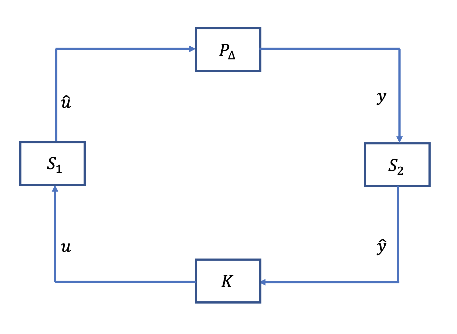
There are two samplers $S_{1}$ and $S_{2}$ in the feedback loop used to sample the output value $y$ of the plant $P_{\Delta}(s)$ and $u$ of the controller $K(s)$ , respectively. The structure of the closed-loop system is depicted in Fig. 1.

3.2 Event-Triggered Mechanism

To save the computation resources and reduce the frequency of the control updating, we adopt the event-triggered sampling mechanism proposed in [Heemels et al., 2012]. Here we will explain specifically how the sampling system operates in the event-triggering mechanism. The sampler $S_{1}$ detects the real output $y$ of the plant $P_{\Delta}(s)$ , and calculates the error between it and the estimate of that output $\hat{y}$ it holds. We use $\epsilon_{y}=\hat{y}-y$ to denote this sampling error. Similarly, the sampler $S_{2}$ detects the real value of the output $u$ of the controller $K(s)$ , holds an estimate of it and calculates the sampling error $\epsilon_{u}=\hat{u}-u$ . A triggering function $f=f(\epsilon_{y},\epsilon_{u},\hat{y},\hat{u},t)$ needs be designed to decide when is the next triggering instant, i.e., when the next sampling has to be done. Typically, we set $f\geq 0$ to indicate the next triggering instant. At the next triggering instant, say $t_{k}$ , the samplers $S_{1}$ and $S_{2}$ update the estimate $\hat{y}$ to $y(t_{k})$ and $\hat{u}$ to $u(t_{k})$ and send them to the controller $K$ and the plant $P_{\Delta}$ , respectively. During the two triggering instants, both the estimate $\hat{y}$ of the output of the plant and the estimate $\hat{u}$ of the output of the controller remain constant.

3.3 Robust Control Objective

Designing a robust feedback controller $K(s)$ as well as the triggering mechanism to stabilize the perturbed system $P_{\Delta}(s)$ is the essential control objective to be handled in this paper. Meanwhile, the closed-loop system must not exhibit Zeno behavior. The stability we need to achieve is the so-called ‘internal stability’ [Zhou & Doyle, 1998], which requires that disturbance injected from any position in the feedback loop shown in Fig. 1 will not lead any divergence phenomenon of the internal signals.

Refer to caption — Figure 1: Block diagram representation of the closed-loop system, where $P_{\Delta}(s)$ is the perturbed linear system to be controlled, $K$ is the controller to be developed, $S_{1}$ and $S_{2}$ are two event-triggered samplers.

4 Robust Event-Triggered Stabilizing Control

4.1 Linear Systems with Additive Uncertainties

In this subsection, we aim to deal with the case where $P_{\Delta}(s)$ can be seen as a nominal linear plant $P_{0}(s)$ perturbed by an additive dynamic uncertainty $\Delta(s)$ , i.e., $P_{\Delta}(s)=P_{0}(s)+\Delta(s)$ with

\Delta(s)=\left[\begin{smallmatrix}\begin{array}[]{c|c}A_{\Delta}&B_{\Delta}\\ \hline\cr C_{\Delta}&D_{\Delta}\end{array}\end{smallmatrix}\right]\in\mathcal{RH}_{\infty}

and $\|\Delta(s)\|_{\infty}\leq\eta$ .

Expressing the above system in the state-space form, we have

	$\displaystyle\dot{x}_{p}$	$\displaystyle=Ax_{p}+B\hat{u},$		(1)
	$\displaystyle y$	$\displaystyle=Cx_{p}+d,$		(1)

and

	$\displaystyle\dot{\xi}$	$\displaystyle=A_{\Delta}\xi+B_{\Delta}\hat{u},$		(2)
	$\displaystyle d$	$\displaystyle=C_{\Delta}\xi,$		(2)

where $x_{p},\xi$ denote the internal states of the nominal linear system $P_{0}(s)$ and the perturbation $\Delta(s)$ , respectively, and $A,B,C,A_{\Delta},B_{\Delta},C_{\Delta}$ are matrices with compatible dimensions.

Also, the controller $K(s)$ can be written in the state-space form as

	$\displaystyle\dot{x}_{k}$	$\displaystyle=A_{k}x_{k}+B_{k}\hat{y},$		(3)
	$\displaystyle u$	$\displaystyle=C_{k}x_{k}+D_{k}\hat{y},$		(3)

where $x_{k}$ denotes the internal state of $K(s)$ . In this section, we adopt the triggering function developed in [Heemels et al., 2012] with some modifications:

f=\begin{bmatrix}\epsilon_{y}\\ \epsilon_{u}\end{bmatrix}^{T}\begin{bmatrix}\epsilon_{y}\\ \epsilon_{u}\end{bmatrix}-\begin{bmatrix}\hat{y}\\ \hat{u}\end{bmatrix}^{T}\begin{bmatrix}\Omega_{1}&\\ &\Omega_{2}\end{bmatrix}\begin{bmatrix}\hat{y}\\ \hat{u}\end{bmatrix}-\mu e^{-\nu t},

(4)

where $\Omega_{1}>0,\Omega_{2}>0,\mu>0,\nu>0$ are the event-triggering parameters to be determined.

It should be noted that the sampling error $\begin{bmatrix}\epsilon_{y}^{T}&\epsilon_{u}^{T}\end{bmatrix}^{T}$ is updated to zero instantly after each triggering instant, then increases during the two triggering instants and will be reset to zero again at the next triggering instant. The triggering condition ensures that the upper bound of the sampling error is closely related to $\hat{y}$ and $\hat{u}$ . Actually, this relationship can be characterized as an affine mapping (operator). The next theorem characterizes this relationship.

Theorem 1.

Define $\epsilon=[\epsilon_{y}^{T},\epsilon_{u}^{T}]^{T}$ and $v=[\hat{y}^{T},\hat{u}^{T}]^{T}$ and $\gamma=\sqrt{\max\{\rho(\Omega_{1}),\rho(\Omega_{2}+\eta^{2}I)\}}$ . It then follows that under the triggering mechanism described in Section 3.2, with the triggering function designed above, we have

\begin{bmatrix}\epsilon(s)\\ d(s)\end{bmatrix}=\Gamma(s)v(s),

where $\Gamma(\cdot)$ is an affine operator whose expression will be given in the proof. Moreover, $\Gamma(\cdot)$ is finite-gain $\mathcal{L}_{2}$ -stable with operator gain $\|\Gamma\|_{\infty}\leq\gamma$ .

Proof 4.1.

When $t\in[t_{k},t_{k+1})$ ,

	$\displaystyle\epsilon_{y}$	$\displaystyle=\hat{y}-y$
		$\displaystyle=-Ce^{A(t-t_{k})}x(t_{k})-\int_{t_{k}}^{t}Ce^{A(t-\tau)}B\hat{u}(\tau)d\tau-d(t)$
		$\displaystyle+\hat{y}.$

Noticing that $d(s)=\Delta(s)\hat{u}(s)$ , thereby by Lemma 1 we have $d(t)=\delta(\hat{u}(t))$ , where $\delta(\cdot)$ is a linear operator in the time domain. Denoting $-\int_{t_{k}}^{t}Ce^{A(t-\tau)}B\hat{u}(\tau)d\tau$ as $\phi(\hat{u}(t))$ with $\phi(\cdot)$ a linear operator. Then it follows that

	$\displaystyle\epsilon_{y}$	$\displaystyle=-Ce^{A(t-t_{k})}x(t_{k})+\phi(\hat{u}(t))-\delta(\hat{u}(t))+\hat{y}(t)$
		$\displaystyle=\phi^{\prime}(\hat{u}(t))+\phi^{\prime\prime}(\hat{y}(t)),$

where $\phi^{\prime}(\cdot)$ and $\phi^{\prime\prime}(\cdot)$ are affine operators in the time domain. Therefore, in light of Lemma 1, we have that $\epsilon_{y}(s)=\Phi_{2}(\hat{u}(s))+\Phi_{1}(\hat{y}(s))=\Phi(v(s))$ where $\Phi_{2}(\cdot)$ , $\Phi_{1}(\cdot)$ and $\Phi(\cdot)$ are affine operators in the frequency domain. Similarly,

	$\displaystyle\epsilon_{u}$	$\displaystyle=\hat{u}-u$
		$\displaystyle=\hat{u}-D_{k}\hat{y}-\int_{t_{k}}^{t}C_{k}e^{A_{k}(t-\tau)}B_{k}\hat{y}(\tau)d\tau$
		$\displaystyle-C_{k}e^{A_{k}(t-t_{k})}x_{k}(t_{k})$
		$\displaystyle=\psi^{\prime\prime}(\hat{u}(t))+\psi^{\prime}(\hat{y}(t)),$

where $\psi^{\prime}(\cdot)$ and $\psi^{\prime\prime}(\cdot)$ are affine operators in the time domain. Therefore, $\epsilon_{u}(s)=\Psi_{1}(\hat{y}(s))+\Psi_{2}(\hat{u}(s))=\Psi(v(s))$ where $\Psi_{1}(\cdot)$ , $\Psi_{2}(\cdot)$ and $\Psi(\cdot)$ are affine operators in the frequency domain. Since $\Delta(s)\in\mathcal{RH}_{\infty}$ , it is definitely an affine operator in the frequency domain. Thus, $d(s)=\Delta(u(s))=\Delta^{\prime}(v(s))$ , where $\Delta^{\prime}(\cdot)$ is also an affine operator in the frequency domain.

Based on the above discussions, we have

\begin{bmatrix}\epsilon(s)\\ d(s)\end{bmatrix}=\begin{bmatrix}\Phi(\cdot)\\ \Psi(\cdot)\\ \Delta^{\prime}(\cdot)\end{bmatrix}v(s)=\Gamma(v(s)),

where $\Gamma(\cdot)=\begin{bmatrix}\Phi(\cdot)\\ \Psi(\cdot)\\ \Delta^{\prime}(\cdot)\end{bmatrix}$ is an affine operator. Next, we prove that the affine-operator $\Gamma(\cdot)$ is finite-gain $\mathcal{L}_{2}$ stable and calculate its $\mathcal{L}_{2}$ norm bound. Since $d(s)=\Delta(s)\hat{u}(s)$ and $\|\Delta\|_{\infty}\leq\eta$ , we have

\int_{-\infty}^{\infty}d^{*}(j\omega)d(j\omega)d\omega\leq\eta^{2}\int_{-\infty}^{\infty}\hat{u}^{*}(j\omega)\hat{u}(j\omega)d\omega.

(5)

From the triggering condition shown in (4), it is clear that

	$\displaystyle\int_{0}^{\infty}f(t)dt=$	$\displaystyle\int_{0}^{\infty}\epsilon^{T}\epsilon dt$
		$\displaystyle-\int_{0}^{\infty}\begin{bmatrix}\hat{y}\\ \hat{u}\end{bmatrix}^{T}\begin{bmatrix}\Omega_{1}&\\ &\Omega_{2}\end{bmatrix}\begin{bmatrix}\hat{y}\\ \hat{u}\end{bmatrix}dt-\frac{\mu}{\nu}\leq 0.$

In light of the Parseval identity [Desoer & Vidyasagar, 1975], it is easy to see that

		$\displaystyle\frac{1}{2\pi}\int_{-\infty}^{\infty}\epsilon^{*}(j\omega)\epsilon(j\omega)d\omega$		(6)
	$\displaystyle\leq$	$\displaystyle\frac{1}{2\pi}\int_{-\infty}^{\infty}\begin{bmatrix}\hat{y}(j\omega)\\ \hat{u}(j\omega)\end{bmatrix}^{*}\begin{bmatrix}\Omega_{1}&\\ &\Omega_{2}\end{bmatrix}\begin{bmatrix}\hat{y}(j\omega)\\ \hat{u}(j\omega)\end{bmatrix}d\omega+\frac{\mu}{\nu}.$		(6)

Adding (5) and (6), we can get that

		$\displaystyle\int_{-\infty}^{\infty}\begin{bmatrix}\epsilon(j\omega)\\ d(j\omega)\end{bmatrix}^{*}\begin{bmatrix}\epsilon(j\omega)\\ d(j\omega)\end{bmatrix}d\omega$		(7)
		$\displaystyle\leq\int_{-\infty}^{\infty}v^{*}(j\omega)\begin{bmatrix}\Omega_{1}&\\ &\Omega_{2}+\eta^{2}I\end{bmatrix}v(j\omega)d\omega+\frac{2\pi\mu}{\nu}$
		$\displaystyle\leq\gamma^{2}\int_{-\infty}^{\infty}v^{*}(j\omega)v(j\omega)d\omega+\frac{2\pi\mu}{\nu}.$

Based on the definition of finite-gain $\mathcal{L}_{2}$ stability and the ${H}_{\infty}$ norm theory, obviously $\Gamma(\cdot)$ is finite-gain $\mathcal{L}_{2}$ stable with operator norm $\|\Gamma\|_{\infty}\leq\gamma$ . $\hfill\square$

Remark 4.2.

This theorem gives an explicit relationship between the sampling error $\epsilon$ and the sampled output value $v$ . The sampling error is, in fact, an image of an affine mapping acting on the sampled output. Notice that this operator can be denoted as $\begin{bmatrix}\Phi(\cdot)\\ \Psi(\cdot)\end{bmatrix}$ and is in general not a transfer function in $\mathcal{RH}_{\infty}$ , but it is finite-gain $\mathcal{L}_{2}$ stable, i.e., it maps a causal $\mathcal{L}_{2}$ signal to another causal $\mathcal{L}_{2}$ signal under the event-triggered mechanism described above.

Remark 4.3.

According to Theorem 1, the system interconnection shown in Fig. 1 is actually equivalent to the system interconnection shown in Fig. 2. The two event-triggered samplers $S_{1}$ and $S_{2}$ in Fig. 1 are equivalent to the two block structure units contained in the two green boxes in Fig. 2. To be more specific, the effect of the sampler $S_{2}$ can be seen as acting on the sampled output $\hat{y}$ and $\hat{u}$ to generate the sampling error $\epsilon_{y}$ , while that of the other sampler $S_{1}$ is to generate $\epsilon_{u}$ . It should be noted that the explicit form of the operators $\Psi(\cdot)$ and $\Phi(\cdot)$ can be very messy and it is in general impossible to express them in a closed form. However, this does not prevent from using the properties of the operators such as $\mathcal{L}_{2}$ stability, since the key quantity we are interested in is the size or norm of the operators, which will be deliberated in the sequal.

Before we proceed to determine the controller parameters and the parameters in the event-triggered mechanism, we first do some transformations to the feedback loop to get some more insightful results. More specifically, we ‘pull out’ the uncertain operator $\Gamma(\cdot)$ . Notice that $\hat{u}=u+\epsilon_{u}$ and $\hat{y}=y+\epsilon_{y}$ , we can then derive that

	$\displaystyle\begin{bmatrix}\dot{x}_{p}\\ \dot{x}_{k}\end{bmatrix}$	$\displaystyle=A_{cl}\begin{bmatrix}x_{p}\\ x_{k}\end{bmatrix}+B_{cl}\begin{bmatrix}\epsilon_{y}\\ \epsilon_{u}\\ d\end{bmatrix},$		(8)
	$\displaystyle\begin{bmatrix}\hat{y}\\ \hat{u}\end{bmatrix}$	$\displaystyle=C_{cl}\begin{bmatrix}x_{p}\\ x_{k}\end{bmatrix}+D_{cl}\begin{bmatrix}\epsilon_{y}\\ \epsilon_{u}\\ d\end{bmatrix},$		(8)

where $A_{cl}=\begin{bmatrix}A+BD_{k}C&BC_{k}\\ B_{k}C&A_{k}\end{bmatrix}$ , $B_{cl}=\begin{bmatrix}BD_{k}&B&BD_{k}\\ B_{k}&0&B_{k}\end{bmatrix}$ , $C_{cl}=\begin{bmatrix}C&0\\ D_{k}C&C_{k}\end{bmatrix}$ , $D_{cl}=\begin{bmatrix}I&0&I\\ D_{k}&I&D_{k}\end{bmatrix}$ .

Denote the system in (8) as $v(s)=M(s)\begin{bmatrix}\epsilon(s)\\ d(s)\end{bmatrix}$ , where $M(s)=\left[\begin{smallmatrix}\begin{array}[]{c|c}A_{cl}&B_{cl}\\ \hline\cr C_{cl}&D_{cl}\end{array}\end{smallmatrix}\right]$ . Combining with the fact that $\begin{bmatrix}\epsilon(s)\\ d(s)\end{bmatrix}=\Gamma(v(s))$ , we then get a classical feedback loop interconnected by a linear system $M(s)$ and a norm-bounded $\mathcal{L}_{2}$ stable but unknown operator $\Gamma(\cdot)$ .

Now we turn back to the major task of designing a stabilizing controller $K(s)=\left[\begin{smallmatrix}\begin{array}[]{c|c}A_{k}&B_{k}\\ \hline\cr C_{k}&D_{k}\end{array}\end{smallmatrix}\right].$ In light of the well-known Small Gain Theorem (Lemma 2), the problem can then be transformed to designing a controller $K(s)$ such that $M(s)\in\mathcal{RH}_{\infty}$ and $\|M(s)\|_{\infty}<\frac{1}{\gamma}$ . This problem can then be coped with by solving a standard $H_{\infty}$ problem. To see this, consider the following linear system:

\begin{bmatrix}z(s)\\ y(s)\end{bmatrix}=P_{add}(s)\begin{bmatrix}w(s)\\ u(s)\end{bmatrix},

where $P_{add}(s)=\left[\begin{smallmatrix}\begin{array}[]{c|cc}A&B_{1}&B_{2}\\ \hline\cr C_{1}&D_{11}&D_{12}\\ C_{2}&D_{21}&D_{22}\end{array}\end{smallmatrix}\right]$ , $B_{1}=\begin{bmatrix}0&B&0\end{bmatrix}$ , $B_{2}=B$ , $C_{1}=\begin{bmatrix}C\\ 0\end{bmatrix}$ , $C_{2}=C$ , $D_{11}=\begin{bmatrix}I&0&I\\ 0&I&0\end{bmatrix}$ , $D_{12}=\begin{bmatrix}0\\ I\end{bmatrix}$ , $D_{21}=\begin{bmatrix}I&0&I\end{bmatrix}$ and $D_{22}=0$ . It is not difficult to verify that

T_{wz}=\mathcal{F}_{l}(P_{0}(s),K(s))=\left[\begin{smallmatrix}\begin{array}[]{c|c}A_{cl}&B_{cl}\\ \hline\cr C_{cl}&D_{cl}\end{array}\end{smallmatrix}\right]=M(s).

Therefore, designing a controller $K(s)$ such that $M(s)$ is stable and $\|M(s)\|_{\infty}<\frac{1}{\gamma}$ is equivalent to designing such a $K(s)$ such that $T_{wz}(s)=\mathcal{F}_{l}(P_{add}(s),K(s))$ is stable and $\|T_{wz}\|_{\infty}=\|\mathcal{F}_{l}(P_{add}(s),K(s))\|_{\infty}<\frac{1}{\gamma}$ . This result can be concluded in the following theorem:

Theorem 2.

Assume that $\gamma>0$ , an event-triggered controller with sampling mechanism shown in Section 3.2, triggering condition shown as (4) and $K(s)=\left[\begin{smallmatrix}\begin{array}[]{c|c}A_{k}&B_{k}\\ \hline\cr C_{k}&D_{k}\end{array}\end{smallmatrix}\right]$ stabilizes any perturbed plant $P_{\Delta}(s)=P_{0}(s)+\Delta(s)$ with $\|\Delta\|_{\infty}\leq\eta$ , if and only if $K(s)$ solves a standard dynamic output feedback $\gamma^{-1}$ -suboptimal $H_{\infty}$ synthesis problem with $P_{add}(s)$ defined as above and $\gamma$ determined by Theorem 1.

Remark 4.4.

Actually, we can further relax our assumption in the sense that the uncertainty $\Delta(s)$ does not even need to be a transfer matrix in $\mathcal{RH}_{\infty}$ . All we need is that $\Delta(s)$ is finite-gain $\mathcal{L}_{2}$ stable. This observation extends the field of application of the developed method provided above.

In light of the above theorem, we can then design the event-triggered controller stabilizing the perturbed system $P_{\Delta}$ . The corresponding parameters $A_{k},B_{k},C_{k},D_{k},\Omega_{1}>0,\Omega_{2}>0$ , $\mu>0$ and $\nu>0$ in the event-triggered controller can be determined via the following algorithm.

Algorithm 1.

An algorithm to find a robust event-triggered protocol for $P_{\Delta}=P_{0}+\Delta$ :

Step 1: Solve the standard $H_{\infty}$ optimal synthesis problem in Theorem 2 and find the optimal $H_{\infty}$ level $\gamma_{opt}$ . If $\gamma_{opt}<\eta^{-1}$ , go to the next step. Otherwise, the robust event-triggered controller may not exist.

Step 2: Choose positive numbers $\mu>0$ , $\nu>0$ . Determine positive-definite matrices $0<\Omega_{1}<\gamma_{opt}^{-2}I$ and $0<\Omega_{2}<(\gamma_{opt}^{-2}-\eta^{2})I$ and calculate $\gamma=\sqrt{\max\{\rho(\Omega_{1}),\rho(\Omega_{2}+\eta^{2}I)\}}$ .

Step 3: Solve the standard $\gamma^{-1}$ -suboptimal $H_{\infty}$ synthesis problem in Theorem 2 to get the controller $K(s)=\left[\begin{smallmatrix}\begin{array}[]{c|c}A_{k}&B_{k}\\ \hline\cr C_{k}&D_{k}\end{array}\end{smallmatrix}\right]$ .

Remark 4.5.

Note that this algorithm eventually transforms the event-triggered robust stabilizing controller synthesis problem to solving a standard $H_{\infty}$ suboptimal control problem with the same order as the original nominal linear plant and that the parameters in the $H_{\infty}$ suboptimal problem all depend on the already-known parameters of the nominal plant. The suboptimal $H_{\infty}$ level to be achieved is determined by the parameters in the triggering mechanism which remains to be developed.

The next theorem shows that the closed-loop system does not exhibit Zeno behavior.

Theorem 3.

The system interconnection resulted by the event-triggering sampling mechanism designed in Section 3.2 and the control protocol designed in Algorithm 1 does not exhibit Zeno behavior.

Proof 4.6.

We will exclude Zeno behavior by contradiction. For simplicity, we assume that $D_{\Delta}=0$ in $\Delta(s)$ .

First, since the closed-loop system is internally stable, then we have that $\zeta=\begin{bmatrix}x_{p}^{T}&x_{k}^{T}&\xi^{T}\end{bmatrix}^{T}$ is a vector with a norm bound, say $H$ . During each time interval between the two consecutive triggering instants, say, $[t_{k},t_{k+1})$ , taking the time derivative of the vector $\zeta$ , we will get that

\displaystyle\dot{\epsilon}=\hat{A}\epsilon+\hat{B}\zeta,

(9)

where

	$\displaystyle\hat{A}$	$\displaystyle=\begin{bmatrix}-CBD_{k}-C_{\Delta}B_{\Delta}D_{k}&-CB-C_{\Delta}B_{\Delta}\\ -C_{k}B_{k}&0\end{bmatrix},$
	$\displaystyle\hat{B}$	$\displaystyle=\begin{bmatrix}\hat{B}_{11}&\hat{B}_{12}&\hat{B}_{13}\\ \hat{B}_{21}&\hat{B}_{22}&\hat{B}_{23}\end{bmatrix},$
	$\displaystyle\hat{B}_{11}$	$\displaystyle=-CA-CBD_{k}C-C_{\Delta}B_{\Delta}D_{k}C,$
	$\displaystyle\hat{B}_{12}$	$\displaystyle=-CBC_{k}-C_{\Delta}B_{\Delta}C_{k},$
	$\displaystyle\hat{B}_{13}$	$\displaystyle=-CBD_{k}C_{\Delta}-C_{\Delta}B_{\Delta}D_{k}C_{\Delta}-C_{\Delta}A_{\Delta},$
	$\displaystyle\hat{B}_{21}$	$\displaystyle=-C_{k}B_{k}C,$
	$\displaystyle\hat{B}_{22}$	$\displaystyle=-C_{k}A_{k},$
	$\displaystyle\hat{B}_{23}$	$\displaystyle=-C_{k}B_{k}C_{\Delta}.$

Suppose that there exists Zeno behavior. Then there is a time instant $T$ such that $\lim_{k\rightarrow\infty}t_{k}=T<\infty$ . This is equivalent to saying that for a small positive real number $\delta=\frac{\mu\|\hat{A}\|}{\|\hat{B}\|^{2}H^{2}}e^{-(4\|\hat{A}\|+\nu)T}$ , there exists such an integer $K$ such that for all $k\geq K$ , we have $t_{k}\in(T-\delta,T]$ . Then we will consider specially the time interval $[t_{K},t_{K+1})$ . Notice that at the triggering instant $t_{K}$ , $\epsilon_{y}$ and $\epsilon_{u}$ are reset to be zero. Since the next triggering time is the first time that $\left\|\epsilon\right\|^{2}$ reaches $v^{T}\left[\begin{smallmatrix}\Omega_{1}&\\ &\Omega_{2}\end{smallmatrix}\right]v+\mu e^{-\nu t},$ there must exist some time instant $T_{0}\in[t_{K},t_{K+1})$ when $\left\|\epsilon(T_{0})\right\|^{2}=\mu e^{-\nu T_{0}}.$ On the other hand,

	$\displaystyle\left\\|\epsilon(T_{0})\right\\|^{2}$	$\displaystyle=\left\\|\int_{t_{K}}^{T_{0}}e^{\hat{A}(T_{0}-\tau)}\hat{B}\zeta(\tau)d\tau\right\\|^{2}$
		$\displaystyle\leq\left\\|e^{\hat{A}(T_{0}-t_{K})}\right\\|^{2}\left\\|\int_{t_{K}}^{T_{0}}e^{-\hat{A}(\tau-t_{K})}\hat{B}\zeta(\tau)d\tau\right\\|^{2}$
		$\displaystyle\leq e^{2\\|\hat{A}\\|T}\left[\int_{t_{K}}^{T_{0}}\left\\|e^{-\hat{A}(\tau-t_{K})}\right\\|\left\\|\hat{B}\zeta(\tau)\right\\|d\tau\right]^{2}.$

According to the well-known Cauthy-Swartz inequality, it then follows that

		$\displaystyle\left\\|\epsilon(T_{0})\right\\|^{2}$
		$\displaystyle\leq e^{2\\|\hat{A}\\|T}\left[\int_{t_{K}}^{T_{0}}e^{2\\|\hat{A}\\|(\tau-t_{K})}d\tau\right]\left[\int_{t_{K}}^{T_{0}}\\|\hat{B}\\|^{2}\\|\zeta(\tau)\\|^{2}d\tau\right]$
		$\displaystyle\leq e^{2\\|\hat{A}\\|T}\frac{1}{2\\|\hat{A}\\|}e^{2\\|\hat{A}\\|(T_{0}-t_{K})}\\|\hat{B}\\|^{2}H^{2}(T_{0}-t_{K})$
		$\displaystyle\leq e^{2\\|\hat{A}\\|T}\frac{1}{2\\|\hat{A}\\|}e^{2\\|\hat{A}\\|T}\\|\hat{B}\\|^{2}H^{2}(T_{0}-t_{K}).$

Notice also that $\mu e^{-\nu T_{0}}\geq\mu e^{-\nu T}$ , therefore we have

T_{0}-t_{K}\geq\frac{2\mu\|\hat{A}\|}{\|\hat{B}\|^{2}H^{2}}e^{-(4\|\hat{A}\|+\nu)T}=2\delta.

This implies that

t_{K+1}-t_{K}>\delta\geq T-t_{K},

which contradicts our assumption. This completes the proof. $\hfill\square$

4.2 Linear Systems with Multiplicative Uncertainties

In this subsection, we consider a linear nominal plant perturbed by a multiplicative uncertainty. Therefore, the perturbed plant has the form $P_{\Delta}(s)=(I+\Delta(s))P_{0}(s)$ with $\Delta(s)\in\mathcal{RH}_{\infty}$ and $\|\Delta(s)\|_{\infty}\leq\eta$ . In light of this, we have

	$\displaystyle\dot{x}_{p}$	$\displaystyle=Ax_{p}+B\hat{u},$		(10)
	$\displaystyle\lambda$	$\displaystyle=Cx_{p},$		(10)

	$\displaystyle\dot{\xi}$	$\displaystyle=A_{\Delta}\xi+B_{\Delta}\lambda,$		(11)
	$\displaystyle d$	$\displaystyle=C_{\Delta}\xi,$		(11)

y=\lambda+d,

(12)

and

	$\displaystyle\dot{x}_{k}$	$\displaystyle=A_{k}x_{k}+B_{k}\hat{y},$		(13)
	$\displaystyle u$	$\displaystyle=C_{k}x_{k}+D_{k}\hat{y},$		(13)

where $\hat{y}$ and $\hat{u}$ denote the sampled value of $y$ and $u$ , respectively. The triggering mechanism is designed to be the same as the one shown in Section 3.2 and we still adopt the static triggering function (4).

Let $\epsilon_{y}=\hat{y}-y$ , $\epsilon_{u}=\hat{u}-u$ , $\tilde{v}=\begin{bmatrix}\lambda^{T}&\hat{y}^{T}&\hat{u}^{T}\end{bmatrix}^{T}$ and $\epsilon=\begin{bmatrix}\epsilon_{y}^{T}&\epsilon_{u}^{T}\end{bmatrix}^{T}$ . Similar to the case where the system is subject to an additive uncertainty, in this case by studying the relationship between the vector $\begin{bmatrix}d^{T}&\epsilon^{T}\end{bmatrix}^{T}$ and the vector $\tilde{v}$ , we have the following result.

Theorem 4.

\begin{bmatrix}d(s)\\ \epsilon(s)\end{bmatrix}=\hat{\Gamma}(s)\tilde{v}(s),

where $\hat{\Gamma}(\cdot)$ is an affine operator which is finite-gain $\mathcal{L}_{2}$ stable. Meanwhile, the operator gain $\|\Gamma\|_{\infty}\leq\hat{\gamma}$ , where $\hat{\gamma}=\sqrt{\max\{\eta^{2},\rho(\Omega_{1}),\rho(\Omega_{2})\}}$ .

Proof 4.7.

The proof is quite similar to that of Theorem 1 and thus is omitted for brevity. $\hfill\square$

On the other hand, combining (10), (11), (12) and (13), we can get that

	$\displaystyle\begin{bmatrix}\dot{x}_{p}\\ \dot{x}_{k}\end{bmatrix}$	$\displaystyle=\hat{A}_{cl}\begin{bmatrix}x_{p}\\ x_{k}\end{bmatrix}+\hat{B}_{cl}\begin{bmatrix}d\\ \epsilon\end{bmatrix},$		(14)
	$\displaystyle\tilde{v}$	$\displaystyle=\hat{C}_{cl}\begin{bmatrix}x_{p}\\ x_{k}\end{bmatrix}+\hat{D}_{cl}\begin{bmatrix}d\\ \epsilon\end{bmatrix},$		(14)

where

	$\displaystyle\hat{A}_{cl}$	$\displaystyle=\begin{bmatrix}A+BD_{k}C&BC_{k}\\ B_{k}C&A_{k}\end{bmatrix},$
	$\displaystyle\hat{B}_{cl}$	$\displaystyle=\begin{bmatrix}BD_{k}&BD_{k}&B\\ B_{k}&B_{k}&0\end{bmatrix},$
	$\displaystyle\hat{C}_{cl}$	$\displaystyle=\begin{bmatrix}C&0\\ C&0\\ D_{k}C&C_{k}\end{bmatrix},$
	$\displaystyle\hat{D}_{cl}$	$\displaystyle=\begin{bmatrix}0&0&0\\ I&I&0\\ D_{k}&D_{k}&0\end{bmatrix}.$

Let $\hat{M}(s)=\left[\begin{smallmatrix}\begin{array}[]{c|c}\hat{A}_{cl}&\hat{B}_{cl}\\ \hline\cr\hat{C}_{cl}&\hat{D}_{cl}\end{array}\end{smallmatrix}\right]$ , we then have $\tilde{v}(s)=\hat{M}(s)\begin{bmatrix}d(s)\\ \epsilon(s)\end{bmatrix}.$ Combining with the fact that $\begin{bmatrix}d(s)\\ \epsilon(s)\end{bmatrix}=\hat{\Gamma}(v(s))$ , we can then get an interconnecting loop consisting of $M(s)$ and $\hat{\Gamma}(\cdot)$ . By the Small Gain Theorem, it is clear that the event-triggered protocol stabilizes the perturbed linear system, if $\hat{M}(s)\in\mathcal{RH}_{\infty}$ and $\|\hat{M}(s)\|_{\infty}<\hat{\gamma}^{-1}$ . This design objective, again, can be transformed to a standard dynamic output $H_{\infty}$ synthesis problem, as will be shown in the next theorem.

Theorem 5.

Given a certain $\hat{\gamma}>0$ , we can then find such an event-triggered controller with

K(s)=\left[\begin{smallmatrix}\begin{array}[]{c|c}A_{k}&B_{k}\\ \hline\cr C_{k}&D_{k}\end{array}\end{smallmatrix}\right]

that makes the closed-loop system (10),(11),(12),(13) internally stable by solving a standard dynamic output $\hat{\gamma}^{-1}$ -suboptimal $H_{\infty}$ synthesis problem with

\hat{P}_{mul}=\left[\begin{smallmatrix}\begin{array}[]{c|cc}A&\hat{B}_{1}&\hat{B}_{2}\\ \hline\cr\hat{C}_{1}&\hat{D}_{11}&\hat{D}_{12}\\ \hat{C}_{2}&\hat{D}_{21}&\hat{D}_{22}\end{array}\end{smallmatrix}\right],

where $\hat{B}_{1}=\begin{bmatrix}0&0&B\end{bmatrix}$ , $\hat{B}_{2}=B$ , $\hat{C}_{1}=\begin{bmatrix}C\\ C\\ 0\end{bmatrix}$ , $\hat{C}_{2}=C$ , $\hat{D}_{11}=\begin{bmatrix}0&0&0\\ I&I&0\\ 0&0&0\end{bmatrix}$ , $\hat{D}_{12}=\begin{bmatrix}0\\ 0\\ I\end{bmatrix}$ , $\hat{D}_{21}=\begin{bmatrix}I&I&0\end{bmatrix}$ and $\hat{D}_{22}=0$ .

Proof 4.8.

The proof is similar to that of Theorem 2 and thus is omitted for brevity. $\hfill\square$

In light of this theorem, we can find such an event-triggered controller with triggering mechanism stated in Section 3.2, triggering condition in (4) and $K(s)=\left[\begin{smallmatrix}\begin{array}[]{c|c}A_{k}&B_{k}\\ \hline\cr C_{k}&D_{k}\end{array}\end{smallmatrix}\right]$ , whose parameters $A_{k}$ , $B_{k}$ , $C_{k}$ , $D_{k}$ , $\Omega_{1}>0$ , $\Omega_{2}>0$ , $\mu>0$ and $\nu>0$ can be determined according to the following algorithm.

Algorithm 2.

An algorithm to find a stabilizing event-triggering controller for $P_{\Delta}=(I+\Delta)P_{0}$ :

Step 1: Solve the standard $H_{\infty}$ optimal synthesis problem in Theorem 5 and find the optimal $H_{\infty}$ level $\kappa_{opt}$ . If $\kappa_{opt}^{-1}\geq\eta$ , go to the next step. Otherwise, the stabilizing event-triggering protocol may not exist.

Step 2: Choose positive numbers $\mu>0$ , $\nu>0$ . Determine positive-definite matrices $0<\Omega_{1}<\kappa_{opt}^{-2}I$ and $0<\Omega_{2}<\kappa_{opt}^{-2}I$ and calculate $\hat{\gamma}=\sqrt{\max\{\eta^{2},\rho(\Omega_{1}),\rho(\Omega_{2})\}}$ .

Step 3: Solve the $\hat{\gamma}^{-1}$ -suboptimal $H_{\infty}$ synthesis problem in Theorem 5 to get the controller $K(s)=\left[\begin{smallmatrix}\begin{array}[]{c|c}A_{k}&B_{k}\\ \hline\cr C_{k}&D_{k}\end{array}\end{smallmatrix}\right]$ .

Theorem 6.

The system interconnection resulted by the event-triggered sampling mechanism shown in subsection 3.2 and the controller designed in Algorithm 2 does not exhibit Zeno behavior.

Proof 4.9.

The proof is omitted for brevity. $\hfill\square$

Remark 4.10.

Similar to the case of additive uncertainty, in the multiplicative uncertainty case the robust stabilizing controller synthesis problem is also transformed into a standard $H_{\infty}$ suboptimal control problem with the same order as the nominal linear plant $P_{0}$ . The only difference lies on the system parameters. Actually, through our operator theoretic approach, more kinds of uncertainties are able to be handled, including the coprime factor uncertainty, and even nonlinear dynamics with Lipschitz constraints, which can also be represented as an $\mathcal{L}_{2}$ stable operator [Green & Limebeer, 2012].

5 Extensions to Dynamic Event-Triggered Mechanisms

In this section, we aim to design an event-triggered controller robust against frequency-domain uncertainties based on the dynamic event-triggered mechanism. To be more specific, inspired by [Antoine, 2015], we adopt the dynamic triggering function described as follows:

\displaystyle f

\displaystyle=\epsilon^{T}\epsilon-v^{T}\begin{bmatrix}\Omega_{1}&\\ &\Omega_{2}\end{bmatrix}v-\chi,

(15)

where $\epsilon$ and $v$ are defined as in Theorem 1, $\chi$ is the internal scalar state with dynamics:

\displaystyle\dot{\chi}

\displaystyle=-\beta\chi-\alpha\left(\epsilon^{T}\epsilon-v^{T}\begin{bmatrix}\Omega_{1}&\\ &\Omega_{2}\end{bmatrix}v\right)

(16)

with $\beta>0$ , $\alpha>0$ and $\chi(0)>0$ . The samplers $S_{1}$ and $S_{2}$ will sample the output of the plant and the controller whenever $f\geq 0$ .

For illustration, in this section we will only consider linear systems perturbed by an additive dynamic uncertainty. The system equation is described as (1) and (2) and the controller is in the form of (3). Interestingly, the introduction of dynamic event-triggering mechanism does not change the conclusion we derive in Theorem 1, as shown in the next theorem.

Theorem 7.

Let $\epsilon$ and $v$ be the vectors defined as in Theorem 1 and $\gamma=\sqrt{\max\{\rho(\Omega_{1}),\rho(\Omega_{2}+\eta^{2}I)\}}$ . Under the dynamic event-triggered mechanism described above with the triggering function shown in (15), we have

\begin{bmatrix}\epsilon(s)\\ d(s)\end{bmatrix}=\Gamma(s)v(s),

where $\Gamma$ is an affine operator which is finite-gain $\mathcal{L}_{2}$ stable. Moreover, $\|\Gamma\|_{\infty}\leq\gamma$ .

Proof 5.11.

Based on the triggering condition, we will always have $f\leq 0$ , which implies

\displaystyle\epsilon^{T}\epsilon-v^{T}\begin{bmatrix}\Omega_{1}&\\ &\Omega_{2}\end{bmatrix}v\leq\chi.

(17)

Therefore, in light of (16), it then follows that

\dot{\chi}\geq-(\beta+\alpha)\chi.

Notice also that $\chi(0)>0$ , by the well-known Comparison Lemma [Khalil, 2001], we have $\chi(t)>0,\forall t>0$ . On the other hand, according to (17), we have

\dot{\chi}\leq-(\beta+\alpha)\left(\epsilon^{T}\epsilon-v^{T}\begin{bmatrix}\Omega_{1}&\\ &\Omega_{2}\end{bmatrix}v\right).

(18)

Integrating (18) from zero to infinity, it then follows that

		$\displaystyle\chi(\infty)\leq\chi(0)$
		$\displaystyle-\int_{0}^{\infty}(\beta+\alpha)\left(\epsilon^{T}\epsilon-v^{T}\begin{bmatrix}\Omega_{1}&\\ &\Omega_{2}\end{bmatrix}v\right)dt.$

Noting that $\chi(\infty)>0$ , we have

\int_{0}^{\infty}\left(\epsilon^{T}\epsilon-v^{T}\begin{bmatrix}\Omega_{1}&\\ &\Omega_{2}\end{bmatrix}v\right)dt\leq\frac{\chi(0)}{\beta+\alpha}.

According to the Passaval Identity [Desoer & Vidyasagar, 1975],

		$\displaystyle\int_{-\infty}^{\infty}\epsilon^{*}(j\omega)\epsilon(j\omega)d\omega$		(19)
		$\displaystyle\leq\int_{-\infty}^{\infty}v(j\omega)^{*}\begin{bmatrix}\Omega_{1}&\\ &\Omega_{2}\end{bmatrix}v(j\omega)d\omega+\frac{2\pi\chi(0)}{\alpha+\beta}$		(19)

Combining with (5), we can get that

		$\displaystyle\int_{-\infty}^{\infty}\begin{bmatrix}\epsilon(j\omega)\\ d(j\omega)\end{bmatrix}^{*}\begin{bmatrix}\epsilon(j\omega)\\ d(j\omega)\end{bmatrix}d\omega$		(20)
		$\displaystyle\leq\int_{-\infty}^{\infty}v^{*}(j\omega)\begin{bmatrix}\Omega_{1}&\\ &\Omega_{2}+\eta^{2}I\end{bmatrix}v(j\omega)d\omega+\frac{2\pi\chi(0)}{\alpha+\beta}$
		$\displaystyle\leq\gamma^{2}\int_{-\infty}^{\infty}v^{*}(j\omega)v(j\omega)d\omega+\frac{2\pi\chi(0)}{\alpha+\beta}.$

Based on the definition of finite-gain $\mathcal{L}_{2}$ stablility and the $\mathcal{H}_{\infty}$ norm theory, it is not difficult to derive that $\Gamma(\cdot)$ is finite-gain $\mathcal{L}_{2}$ stable and $\|\Gamma\|_{\infty}\leq\gamma$ . $\hfill\square$

Remark 5.12.

This theorem tells that for a linear system perturbed by an additive dynamic uncertainty, the effect of the aforementioned dynamic event-triggered controller is the same as that of the static event triggering protocol. Therefore, the result of Theorem 2 can be directly applied to the dynamic event-triggered case. Moreover, the dynamic event-triggered robust stabilization problem can still be solved using Algorithm 1 with triggering mechanism and triggering function replaced correspondingly. It is also very similar to exclude Zeno behavior. Although here we only consider the linear system subject to an additive dynamic uncertainty, it is not difficult to see that for a linear system perturbed by other types of uncertainties, similar conclusions still hold and similar algorithms can still work.

6 General IQC-Based Event-Triggered Mechanisms

From the above discussion, we know that no matter the triggering condition is static or dynamic, as long as it gives a constraint that preserves the operator $\Gamma(\cdot)$ (the operator which maps $v(s)$ to $\begin{bmatrix}\epsilon(s)\\ d(s)\end{bmatrix}$ ) a finite $\mathcal{L}_{2}$ gain, the event-triggered robust stabilization problem can then be transformed into the classical problem in the robust control theory. On the other hand, as pointed out in [Megretski et al., 1997], the small gain condition is a specialization of the integral quadratic constraints (IQC). Thus it is natural to ask whether the above ‘finite $\mathcal{L}_{2}$ gain preserving’ triggering condition can be generalized to some triggering condition that characterizes quadratic constraint between $\begin{bmatrix}\epsilon(s)\\ d(s)\end{bmatrix}$ and $v(s)$ .

To be more specific, we can rewrite (20) as

\displaystyle\int_{-\infty}^{\infty}\begin{bmatrix}v(j\omega)\\ w(j\omega)\end{bmatrix}^{*}\begin{bmatrix}\Omega&\\ &-I\end{bmatrix}\begin{bmatrix}v(j\omega)\\ w(j\omega)\end{bmatrix}d\omega+\frac{2\pi\chi(0)}{\alpha+\beta}\geq 0,

(21)

where $w(j\omega)=\begin{bmatrix}\epsilon(j\omega)\\ d(j\omega)\end{bmatrix}$ and $\Omega=\begin{bmatrix}\Omega_{1}&\\ &\Omega_{2}+\eta^{2}I\end{bmatrix}$ . Inspired by [Megretski et al., 1997], one can naturally ask: What if the Hermitian matrix $\begin{bmatrix}\Omega\\ &-I\end{bmatrix}$ is replaced by a more general one $\Pi=\begin{bmatrix}\Pi_{1}&\Pi_{2}\\ \Pi_{2}^{*}&\Pi_{3}\end{bmatrix}$ or even a dynamical one $\Pi(\omega)=\begin{bmatrix}\Pi_{1}(\omega)&\Pi_{2}(\omega)\\ \Pi_{2}^{*}(\omega)&\Pi_{3}(\omega)\end{bmatrix}$ ? Due to the existence of the positive defect term $\frac{2\pi\chi(0)}{\alpha+\beta}$ , the answer is: Only the ‘small-gain’ like IQC can be used here. That is, $\Pi(j\omega)=\begin{bmatrix}\Pi_{1}(\omega)&\Pi_{2}(\omega)\\ \Pi_{2}^{*}(\omega)&\Pi_{3}(\omega)\end{bmatrix}$ with $\Pi_{1}(\omega)>0$ and $\Pi_{3}(\omega)<0$ . This result is concluded as the following lemma:

Lemma 6.13.

(Internal stability criterion based on IQC with defect) Assume that $G(s)\in\mathcal{RH}_{\infty}$ and signals $w$ and $v$ are in the $\mathcal{L}_{2}$ space. Suppose that $v(s)=G(s)w(s)$ and $w(s)=\Delta(v(s))$ , where $\Delta(\cdot)$ is a bounded causal operator, and they satisfy the following IQC condition with defect $\xi>0$ defined by $\Pi$ :

\displaystyle\int_{-\infty}^{\infty}\begin{bmatrix}v(j\omega)\\ w(j\omega)\end{bmatrix}^{*}\begin{bmatrix}\Pi_{1}(\omega)&\Pi_{2}(\omega)\\ \Pi_{2}^{*}(\omega)&\Pi_{3}(\omega)\end{bmatrix}\begin{bmatrix}v(j\omega)\\ w(j\omega)\end{bmatrix}d\omega+\xi\geq 0

(22)

with $\Pi_{1}(\omega)>0$ and $\Pi_{3}(\omega)<0$ , $\forall\omega\in\mathbf{R}$ , two Hermitian valued matrices with compatible dimensions. Then, if

\begin{bmatrix}G(j\omega)\\ I\end{bmatrix}^{*}\begin{bmatrix}\Pi_{1}(\omega)&\Pi_{2}(\omega)\\ \Pi_{2}^{*}(\omega)&\Pi_{3}(\omega)\end{bmatrix}\begin{bmatrix}G(j\omega)\\ I\end{bmatrix}<0,\quad\forall\omega\in\mathbf{R},

(23)

then the system interconnection of $G$ and $\Delta$ is internally stable.

Proof 6.14.

Since $\Pi_{1}(\omega)>0$ and $\Pi_{3}(\omega)<0$ $\forall\omega\in\mathbf{R}$ , it is easy to verify that $\begin{bmatrix}\Pi_{1}(\omega)&\Pi_{2}(\omega)\\ \Pi_{2}^{*}(\omega)&\Pi_{3}(\omega)\end{bmatrix}$ is congruent to $\begin{bmatrix}I&0\\ 0&-I\end{bmatrix}$ , i.e., there exists a nonsingular matrix $C(j\omega)$ such that

\begin{bmatrix}\Pi_{1}(\omega)&\Pi_{2}(\omega)\\ \Pi_{2}^{*}(\omega)&\Pi_{3}(\omega)\end{bmatrix}=C^{*}(j\omega)\begin{bmatrix}I&0\\ 0&-I\end{bmatrix}C(j\omega)\quad\forall\omega\in\mathbf{R}.

Let $\begin{bmatrix}\tilde{v}(j\omega)\\ \tilde{w}(j\omega)\end{bmatrix}=C(j\omega)\begin{bmatrix}v(j\omega)\\ w(j\omega)\end{bmatrix}$ and denote $\tilde{w}=\tilde{\Delta}(\tilde{v})$ , it then follows from (22) that

\|\tilde{w}\|_{2}^{2}\leq\|\tilde{v}\|_{2}^{2}+\frac{\xi}{2\pi}.

(24)

Therefore $\|\tilde{\Delta}\|_{\infty}\leq 1$ . In light of Small Gain Theorem (Lemma 2), the closed-loop system is internally stable if

\begin{bmatrix}\tilde{G}(j\omega)\\ I\end{bmatrix}^{*}\begin{bmatrix}I&0\\ 0&-I\end{bmatrix}\begin{bmatrix}\tilde{G}(j\omega)\\ I\end{bmatrix}<0\quad\forall\omega\in\mathbf{R},

(25)

where $\tilde{G}(j\omega)$ denotes the transfer matrix from $\tilde{w}$ to $\tilde{v}$ . Noticing that $\begin{bmatrix}0&\tilde{G}(j\omega)\\ 0&I\end{bmatrix}\begin{bmatrix}\tilde{v}\\ \tilde{w}\end{bmatrix}=C(j\omega)\begin{bmatrix}0&G(j\omega)\\ 0&I\end{bmatrix}\begin{bmatrix}v\\ w\end{bmatrix}$ and $\begin{bmatrix}v\\ w\end{bmatrix}=C^{-1}(j\omega)\begin{bmatrix}\tilde{v}\\ \tilde{w}\end{bmatrix}$ , we have

	$\displaystyle\begin{bmatrix}\tilde{G}(j\omega)\\ I\end{bmatrix}$	$\displaystyle=C(j\omega)\begin{bmatrix}0&G(j\omega)\\ 0&I\end{bmatrix}C^{-1}(j\omega)\begin{bmatrix}0\\ I\end{bmatrix}$
		$\displaystyle=C(j\omega)\begin{bmatrix}G(j\omega)\\ I\end{bmatrix}\begin{bmatrix}0&I\end{bmatrix}C^{-1}(j\omega)\begin{bmatrix}0\\ I\end{bmatrix}$
		$\displaystyle=C(j\omega)\begin{bmatrix}G(j\omega)\\ I\end{bmatrix}D(j\omega)$

and $D(j\omega)$ is nonsingular $\forall\omega\in\mathbf{R}$ . Therefore, (25) is equivalent to (23). $\hfill\square$

Remark 6.15.

It is not difficult to see that we can relax the condition $\Pi_{1}(\omega)>0$ to $\Pi_{1}(\omega)\geq 0$ while not change the result derived above.

Remark 6.16.

This lemma extends the results in the classical IQC-based internal stability theorem in [Megretski et al., 1997] in the sense that here we allow a defect term $\xi$ in the quadratic functional. However, a stronger constraint of the positivity has to be imposed on the matrices $\Pi_{1}(\omega)$ and $-\Pi_{3}(\omega)$ . In short, only when the IQC is ‘small-gain’ like can we introduce a defect term in the quadratic functional while remain the internal stability condition unchanged. The defect term corresponds to the additional term $\chi$ in the event-triggered condition and is critical and indispensable since we have to exclude Zeno behavior.

Now, we are ready to put forward the IQC-based dynamic event-triggered control algorithm that is robust against additive dynamic uncertainty described in (2).

Algorithm 3.

An algorithm to find a robust IQC based dynamic event-triggered protocol for $P_{\Delta}=P_{0}+\Delta$ :

Step 1: Solve the standard optimal $H_{\infty}$ synthesis problem in Theorem 2 and find the optimal $H_{\infty}$ level $\gamma_{opt}$ . If $\gamma_{opt}\eta<1$ , go to the next step . Otherwise the robust stabilizing event-triggered controller may not exist.

Step 2: Select a $\mathbf{C}^{(p+q)}\mapsto\mathbf{C}^{(p+q)}$ square transfer matrix $G_{1}(j\omega)=\left[\begin{smallmatrix}\begin{array}[]{c|c}A_{1}&B_{1}\\ \hline\cr C_{1}&D_{1}\end{array}\end{smallmatrix}\right]\in\mathcal{RH}_{\infty}$ such that $\|G_{1}(j\omega)\|_{\infty}^{2}=\sigma_{1}^{2}<\gamma_{opt}^{-2}-\eta^{2}$ and let $\bar{v}(t)\in\mathbf{R}^{p+q}:=\left[\begin{smallmatrix}\begin{array}[]{c|c}A_{1}&B_{1}\\ \hline\cr C_{1}&D_{1}\end{array}\end{smallmatrix}\right]v(t)$ (Here $v(t)$ is defined as in Theorem 1).

Step 3: Select a nonsingular square transfer matrix $G_{2}(j\omega)=\left[\begin{smallmatrix}\begin{array}[]{c|c}A_{2}&B_{2}\\ \hline\cr C_{2}&D_{2}\end{array}\end{smallmatrix}\right]\in\mathcal{RH}_{\infty}$ such that $D_{2}$ is nonsingular and $\|G_{2}(j\omega)\|_{\infty}\leq 1$ . Denote $\bar{\epsilon}(t)\in\mathbf{R}^{p+q}:=\left[\begin{smallmatrix}\begin{array}[]{c|c}A_{2}-B_{2}D_{2}^{-1}C_{2}&B_{2}D_{2}^{-1}\\ \hline\cr D_{2}^{-1}C_{2}&D_{2}^{-1}\end{array}\end{smallmatrix}\right]\begin{bmatrix}\epsilon_{y}\\ \epsilon_{u}\end{bmatrix}$ , that is $\bar{\epsilon}(s)=G_{2}(s)^{-1}\epsilon(s)$ .

Step 4: Set the triggering function to be

f=\bar{\epsilon}(t)^{T}\bar{\epsilon}(t)-\bar{v}(t)^{T}\bar{v}(t)-\chi(t)

with $\chi(0)>0$ and

\dot{\chi}(t)=-\beta\chi(t)-\alpha(\bar{\epsilon}(t)^{T}\bar{\epsilon}(t)-\bar{v}(t)^{T}\bar{v}(t)),

where $\beta>0$ and $\alpha>0$ . When $f\geq 0$ at time $t_{k}$ , the sampler $S_{1}$ and $S_{2}$ samples the output of the plant ( $y(t_{k})$ ) and the output of the controller ( $u(t_{k})$ ) respectively, i.e., $\hat{y}$ is set to be $y(t_{k})$ , $\hat{u}$ is set to be $u(t_{k})$ , and $\epsilon_{y}$ and $\epsilon_{u}$ are reset to be $0$ . Otherwise, $\hat{y}$ and $\hat{u}$ remain unchanged while $\epsilon_{y}=\hat{y}-y(t)$ and $\epsilon_{u}=\hat{u}-u(t)$ .

Step 5: Choose $\gamma_{opt}<\gamma<\frac{1}{\sqrt{\sigma_{1}^{2}+\eta^{2}}}$ and solve the $\gamma$ -suboptimal $H_{\infty}$ problem in Theorem 2 and get the controller $K(s)=\left[\begin{smallmatrix}\begin{array}[]{c|c}A_{k}&B_{k}\\ \hline\cr C_{k}&D_{k}\end{array}\end{smallmatrix}\right]$ .

The next Theorem shows the effectivity of the aforementioned event-triggered controller design algorithm.

Theorem 8.

For the linear system (1) subject to the additive dynamic uncertainty (2) with $H_{\infty}$ norm bound $\eta$ , if we apply the event-triggering mechanism and the controller $K(s)$ designed in Algorithm 3, then the closed-loop system is internally stable. Moreover, no Zeno behavior exhibits.

Proof 6.17.

Following the proof of Theorem 7, it is not difficult to derive that

\int_{0}^{+\infty}(\bar{\epsilon}^{T}(t)\bar{\epsilon}(t)-\bar{v}^{T}(t)\bar{v}(t))dt\leq\dfrac{\chi(0)}{\alpha+\beta}.

Therefore, we have

\int_{-\infty}^{\infty}\begin{bmatrix}\bar{v}(j\omega)\\ \bar{\epsilon}(j\omega)\end{bmatrix}^{*}\begin{bmatrix}I&0\\ 0&-I\end{bmatrix}\begin{bmatrix}\bar{v}(j\omega)\\ \bar{\epsilon}(j\omega)\end{bmatrix}d\omega+\frac{2\pi\chi(0)}{\alpha+\beta}\geq 0.

Notice that $\begin{bmatrix}\bar{v}(j\omega)\\ \bar{\epsilon}(j\omega)\end{bmatrix}=\begin{bmatrix}G_{1}(j\omega)&0\\ 0&G_{2}^{-1}(j\omega)\end{bmatrix}\begin{bmatrix}v(j\omega)\\ \epsilon(j\omega)\end{bmatrix}$ , it then follows that

\int_{-\infty}^{\infty}\begin{bmatrix}v(j\omega)\\ \epsilon(j\omega)\end{bmatrix}^{*}\begin{bmatrix}\Psi_{1}(\omega)&0\\ 0&-\Psi_{2}(\omega)\end{bmatrix}\begin{bmatrix}v(j\omega)\\ \epsilon(j\omega)\end{bmatrix}d\omega+\frac{2\pi\chi(0)}{\alpha+\beta}\geq 0

(26)

with $\Psi_{1}(\omega)=G_{1}^{*}(j\omega)G_{1}(j\omega)\geq 0$ and $\Psi_{2}(\omega)=G_{2}^{-*}(j\omega)G_{2}^{-1}(j\omega)>0$ , $\forall\omega\in\mathbf{R}$ . On the other hand, in light of (5),

\int_{-\infty}^{\infty}(v^{*}(j\omega)\eta^{2}Iv(j\omega)-d^{*}(j\omega)d(j\omega))d\omega\geq 0.

Combining with (26), we then have

		$\displaystyle\int_{-\infty}^{\infty}\begin{bmatrix}v(j\omega)\\ \epsilon(j\omega)\\ d(j\omega)\end{bmatrix}^{*}\begin{bmatrix}\Psi_{1}(\omega)+\eta^{2}I&&\\ &-\Psi_{2}(\omega)&\\ &&-I\end{bmatrix}\begin{bmatrix}v(j\omega)\\ \epsilon(j\omega)\\ d(j\omega)\end{bmatrix}d\omega$		(27)
		$\displaystyle+\frac{2\pi\chi(0)}{\alpha+\beta}\geq 0.$		(27)

Applying Lemma 6.13, the system is internally stable, if

\displaystyle\begin{bmatrix}M(j\omega)\\ I\end{bmatrix}^{*}\begin{bmatrix}\Psi_{1}(\omega)+\eta^{2}I&&\\ &-\Psi_{2}(\omega)&\\ &&-I\end{bmatrix}\begin{bmatrix}M(j\omega)\\ I\end{bmatrix}<0

(28)

$\forall\omega\in\mathbf{R}.$ This condition holds if and only if

M^{*}(j\omega)(\Psi_{1}(\omega)+\eta^{2}I)M(j\omega)<\begin{bmatrix}\Psi_{2}(\omega)&\\ &I\end{bmatrix},

which is equivalent to

		$\displaystyle\begin{bmatrix}G_{2}^{}(j\omega)&\\ &I\end{bmatrix}M^{}(j\omega)(G_{1}^{*}(j\omega)G_{1}(j\omega)+\eta^{2}I)M(j\omega)$		(29)
		$\displaystyle\times\begin{bmatrix}G_{2}(j\omega)&\\ &I\end{bmatrix}<I.$		(29)

When the event triggering mechanism and the controller $K(s)$ is designed as in the Algorithm 3, we have $\|G_{2}(j\omega)\|_{\infty}\leq 1$ and meanwhile

\sqrt{\|G_{1}(j\omega)\|^{2}_{\infty}+\eta^{2}}\|M(j\omega)\|_{\infty}<1.

It is easy to verify that (29) holds. Thus the closed-loop system is internally stable. The excluding of the Zeno behavior is similar to the proof of Theorem 3 and thus is omitted for brevity. $\hfill\square$

Remark 6.18.

Actually, as shown in (26), the event-triggered protocol designed in Algorithm 3 establishes a more general IQC compared to the one shown in (21). The to-be-developed dynamical systems $G_{1}(s)$ and $G_{2}(s)$ endow a great amount of flexibility and degree of freedom to the controller design and the performance optimization.

7 Simulation Results

In this section, a design example is illustrated for a linear system with additive uncertainty to manifest the effectiveness of the proposed algorithm. Consider the following strictly proper linear system:

P(s)=\left[\begin{smallmatrix}\begin{array}[]{cc|c}-12.5&5.9&1\\ -7.1&13.8&2\\ \hline\cr-4&5.5&0\end{array}\end{smallmatrix}\right]

and assume that the additive perturbation is of the form:

\Delta(s)=\left[\begin{smallmatrix}\begin{array}[]{cc|c}-15.4&10.7&-1.24\\ -15.7&-1.41&-1.28\\ \hline\cr 1.165&-2.07&0\end{array}\end{smallmatrix}\right].

It is easy to calculate that $\|\Delta\|_{\infty}=\eta=0.1112$ .

7.1 Verifying the effectiveness of Algorithm 1

Based on Algorithm 1, by solving the standard optimal $H_{\infty}$ synthesis problem in Theorem 2, we find that the optimal $H_{\infty}$ level $\lambda_{opt}=3.0683<\eta^{-1}$ . Therefore the robust stabilization problem is solvable. Following Step $1$ , we set $\mu=0.1$ , $\nu=5$ , $\Omega_{1}=\lambda_{opt}^{-2}\times 0.98=0.1041$ and $\Omega_{2}=(\lambda_{opt}^{-2}-\eta^{2})\times 0.98=0.0920$ . It is then easy to derive that $\gamma=0.3230$ . Solving the $\gamma^{-1}$ -suboptimal $H_{\infty}$ synthesis problem, we can then get a controller

K(s)=\left[\begin{smallmatrix}\begin{array}[]{c|c}-11.9130&-0.7953\\ \hline\cr-3.5437&-1.8130\end{array}\end{smallmatrix}\right].

Applying the controller and event-triggered mechanism designed as above, we then depict the evolution of the internal states $x_{p}$ and $x_{k}$ with time. As shown in Fig. 3, the closed-loop system is internally stabilized by the designed event-triggered control law. Moreover, we depict the evolution of $\|\epsilon\|$ and $\sqrt{\|v\|^{2}+\mu e^{-\nu t}}$ between $0s$ to $1.5s$ in Fig. 4 whose intersections represent the triggering instants. This figure shows clearly that there is no Zeno behavior.

7.2 Verifying the effectiveness of Algorithm 3

Next, we move on to test the effectivity of the Algorithm 3. We still consider the plant $P(s)$ subject to additive dynamic uncertainty $\Delta(s)$ in the previous case. Based on Step $1$ , the robust event-triggered stabilization problem is solvable. In Step $2$ and Step $3$ , we set

G_{1}=\left[\begin{smallmatrix}\begin{array}[]{cc|cc}-1.9&6.7&0.1019&-0.2209\\ -4.3&-10.4&0.7561&-0.4842\\ \hline\cr 0.3&-4.1&0.0025&0\\ 0.58&0.39&0.0671&0.1529\end{array}\end{smallmatrix}\right]

and

G_{2}=\left[\begin{smallmatrix}\begin{array}[]{cc|cc}-19&16.7&0.2&-2.6\\ -43&0.4&1.9&-0.57\\ \hline\cr 0.064&0.8743&0.7677&0\\ 0.1237&-0.0832&0.0671&-0.5118\end{array}\end{smallmatrix}\right].

Note that $\|G_{1}\|_{\infty}=\sqrt{0.95(\gamma_{opt}^{-2}-\eta^{2})}=0.2986$ and $\|G_{2}\|_{\infty}=0.9<1$ . The initial value of the internal state of $G_{1}$ and $G_{2}^{-1}$ is randomly chosen. In Step $4$ , we set $\alpha=2.5$ , $\beta=1.0$ and randomly choose a positive $\chi(0)$ . In Step $5$ , we set $\gamma=0.8(\frac{1}{\sqrt{\|G_{1}\|_{\infty}^{2}+\eta^{2}}}-\gamma_{opt})+\gamma_{opt}=3.1244$ . Solving the $\gamma$ -suboptimal $H_{\infty}$ problem in Theorem 2, we can get that

K(s)=\left[\begin{smallmatrix}\begin{array}[]{cc|c}-9.0230&126.3555&0.7510\\ -324.2813&-14216&-174.0507\\ \hline\cr-0.1597&148.4024&0\\ \end{array}\end{smallmatrix}\right].

Applying the controller and the event-triggered mechanism developed here, we can then draw the evolution of the internal states $x_{p}$ and $x_{k}$ from $0s$ to $6s$ in Fig. 5. It is clear from Fig. 5 that the closed-loop system is internally stable.

To show that the closed-loop system does not exhibit Zeno behavior, we draw the evolution of $\|\epsilon\|$ and $\sqrt{\|v\|^{2}+\chi}$ respectively from $0s$ to $3s$ in Fig. 6. The triggering instants are their intersections and it is clear that there is no Zeno behavior.

8 Conclusion

In this paper, we have established an operator-theoretic approach for the robust event-triggered control problem of general linear systems subject to frequency-domain uncertainties. By showing that under the typical static and dynamic, and even the generalized IQC-based event triggering mechanisms, the mapping from sampled outputs to sampling errors are essentially finite-gain $\mathcal{L}_{2}$ stable affine operators, robust event-triggered control laws can be systematically designed by solving the standard $H_{\infty}$ synthesis problem of a modified linear system.

There are many potential extensions to the present work, e.g., considering the robust $H_{2}$ and $H_{\infty}$ performance of event-triggered controllers and designing robust consensus event-triggered protocols for linear or nonlinear multi-agent systems.

References

[Chen et al., 1991] Chen, T., & Francis, B.A. (1991). Input-output stability of sampled-data systems. IEEE Transactions on Automatic Control, 36(1), 50–58.
[Astrom & Bernhardsson, 1999] Astrom, K. J., & Bernhardsson, B. (1999). Comparison of periodic and event based sampling for first order stochastic systems. In 14th IFAC world congress, Vol. 11, Cape Town, South Africa. (pp.301–306).
[Heemels et al., 2012] Heemels, W. P. M. H., Johansson, K.-H., & Tabuada, P. (2012). An introduction to event-triggered and self-triggered control. In 51st IEEE conference on decision and control, Maui, Hawaii, USA (pp. 3270–3285).
[Miskowicz, 2015] Miskowicz, M.(2015). Event-based control and signal processing. CRC Press.
[Laurentiu et al., 2017] Laurentiu, H., Christophe, F., Hassan, O., Alexandre, S., Emilia, F., Jean-Pierre, R., Silviu, I. N. (2017). Recent developments on the stability of systems with aperiodic sampling: An overview. Automatica , 76 (2017), 309–335.
[Henningsson et al., 2008] Henningsson, T., Johannesson, E., & Cervin, A. (2008). Sporadic event-based control of first-order linear stochastic systems. Automatica , 44 (2008), 2890–2895.
[Lunze & Lehmann, 2010] Lunze, J., & Lehmann, D. (2010). A state-feedback approach to event-based control. Automatica , 46 (2010), 211–215.
[Gawthrop & Wang, 2009] Gawthrop, P. J., & Wang. L. B. (2009). Event-driven intermittent control. International Journal of Control , 82 (2009), 2235–2248.
[Donkers & Heemels, 2012] Donkers, M. C. F., & Heemels, W. P. M. H. (2012). Output-based event-triggered control with guaranteed $\mathcal{L}_{\infty}$ -gain improved and decentralized event-triggering. IEEE Transactions on Automatic Control, 57(6), 1362–1376.
[Dolk et al., 2017] Dolk, V. S., Borgers, D. P., & Heemels, W. P. M. H. (2017). Output-based and decentralized dynamic event-triggered control with guaranteed $\mathcal{L}_{p}$ -gain performance and zeno-freeness. IEEE Transactions on Automatic Control, 62(1), 34–49.
[Postoyan et al., 2015] Postoyan, R., Tabuada, P., Nesic, D., & Anta. A. (2015). A framework for the event triggered stabilization of nonlinear systems. IEEE Transactions on Automatic Control, 60(4), 982–996.
[Liu et al., 2021] Liu, K. Z., Teel, A. R., Sun, X. M., & Wang, X. F. (2021). Model-based dynamic event-triggered control for systems with uncertainty: A hybrid system approach. IEEE Transactions on Automatic Control, 66(1), 444–451.
[Xing et al., 2019] Xing, L., Wen, C., Liu, Z., Su, H., & Cai, J. (2019). Event-triggered output feedback control for a class of uncertain nonlinear systems. IEEE Transactions on Automatic Control, 64(1), 290–297.
[Ristevski et al., 2021] Ristevski, S., Yucelen, T., & Muse, J. A. (2021). An event triggered distributed control architecture for scheduling information exchange in networked multiagent systems. IEEE Transactions on Control Systems Technology, in publication.
[Nowzari et al., 2019] Nowzari, C., Garcia, E., & Cortes, J. (2019). Event-triggered communication and control of networked systems for multi-agent consensus. Automatica, 105(2019), 1–27.
[Ding et al., 2018] Ding, L., Han, Q. L., Ge, X., & Zhang, X., M. (2018). An overview of recent advances in event triggered consensus of multi-agent systems. IEEE Transactions on Automatic Control, 64(1), 290–297.
[Xiao et al., 2021] Xiao, F., Shi, Y., & Chen, T. (2021). Robust stability of networked linear control systems with asynchronous continuous- and discrete-time event-triggering schemes. IEEE Transactions on Automatic Control, 66(2), 932–939.
[Tripathy et al., 2017] Tripathy, N. S., Kar, I. N., & Paul, K. (2017). “Stabilization of uncertain discrete-time linear system with limited communication,” IEEE Transactions on Automatic Control, 62(9), pp. 4727–4733, 2017.
[Seuret et al., 2019] Seuret, A., Prieur, C., Tarbouriech, S., Teel, A. R., & Zaccarian, L. (2019). “A nonsmooth hybrid invariance principle applied to robust event-triggered design,” IEEE Transactions on Automatic Control , 64(5), pp. 2061–2068.
[Antoine, 2015] Antoine, G. (2015). Dynamic triggering mechanisms for event-triggered control. IEEE Transactions on Automatic Control, 60(7), 1992–1997.
[Tripathy et al., 2017] Tripathy, N. S., Kar, I. N., Paul, K. (2017). Stabilization of uncertain discrete-time linear system with limited communication. IEEE Transactions on Automatic Control, 62(9), 4727–4733.
[Seuret et al., 2019] Seuret, A., Prieur, C., Tarbouriech, S., Teel, A. R., and Zaccarian, L. (2019). A nonsmooth hybrid invariance principle applied to robust event–triggered design. IEEE Transactions on Automatic Control, 64(5), 2061–2068.
[Desoer & Vidyasagar, 1975] Desoer, C. A. & Vidyasagar, M. (1975) Feedback Systems: Input-Output Properties. Academic Press, New York, 1975.
[Zhou & Doyle, 1998] Zhou, K and Doyle, J. C. (1998) Essentials of Robust Control. Prentice Hall, Upper Saddle River, NJ, 1998.
[Megretski et al., 1997] Megretski, A., Rantzer, A. (1997). System analysis via integral quadratic constraints. IEEE Transactions on Automatic Control, 42(6), 819–830.
[Wang & Lemmon, 2011] Wang, X., & Lemmon, M. D. (2011). Event-triggering distributed networked control systems. IEEE Transactions on Automatic Control, 56(3), 586–601.
[Tabuada, 2007] Tabuada, P. (2007). Event-triggered real-time scheduling of stabilizing control tasks. IEEE Transactions on Automatic Control, 52(9), 1680–1685.
[Khalil, 2001] Khalil, H. K. (2001). Nonlinear Systems . Prentice Hall, Upper Saddle River, NJ, 2001.
[Green & Limebeer, 2012] Green, M., & Limebeer, J.N., D. (2012).Linear Robust Control. Dover Publications, Mineola, New York, 2012.
[Tarbouriech et al., 2018] Tarbouriech, S., Seuret, A., Prieur, C., and Zaccarian, L. (2018). Insights on event-triggered control for linear systems subject to norm-bounded uncertainty. In Control Subject to Computational and Communication Constraints, pages 181–196. Springer, 2018.
[Xing et al., 2020] Xing, W., Shi, P., Agarwal, R. K., and Li, L. (2020). Robust $H_{\infty}$ Pinning synchronization for complex networks with event–triggered communication scheme. IEEE Transactions on Circuits and Systems-I: Regular Papers, 67(12), 5233–5245.
[Kishida, 2019] Kishida, M. (2019). Event–triggered control with self-triggered sampling for discrete–time uncertain systems. IEEE Transactions on Automatic Control, 64(3), 1273–1279.
[Huong et al., 2020] Huong, D. C., Huynh, V. T., and Trinh, H. (2020). On static and dynamic triggered mechanisms for event–triggered control of uncertain systems. Circuits, Systems, and Signal Processing, 39(10), 5020–5038.
[Zhang et al., 2021] Zhang, S., Lv, Y., and Li, Z. (2021). An operator-theoretic approach to robust event-triggered control of network systems with frequency-domain uncertainties. IEEE Transactions on Automatic Control, submitted for publication.

	$\displaystyle\left\\|\epsilon(T_{0})\right\\|^{2}$	$\displaystyle=\left\\|\int_{t_{K}}^{T_{0}}e^{\hat{A}(T_{0}-\tau)}\hat{B}\zeta(\tau)d\tau\right\\|^{2}$
		$\displaystyle\leq\left\\|e^{\hat{A}(T_{0}-t_{K})}\right\\|^{2}\left\\|\int_{t_{K}}^{T_{0}}e^{-\hat{A}(\tau-t_{K})}\hat{B}\zeta(\tau)d\tau\right\\|^{2}$
		$\displaystyle\leq e^{2\\|\hat{A}\\|T}\left[\int_{t_{K}}^{T_{0}}\left\\|e^{-\hat{A}(\tau-t_{K})}\right\\|\left\\|\hat{B}\zeta(\tau)\right\\|d\tau\right]^{2}.$

		$\displaystyle\left\\|\epsilon(T_{0})\right\\|^{2}$
		$\displaystyle\leq e^{2\\|\hat{A}\\|T}\left[\int_{t_{K}}^{T_{0}}e^{2\\|\hat{A}\\|(\tau-t_{K})}d\tau\right]\left[\int_{t_{K}}^{T_{0}}\\|\hat{B}\\|^{2}\\|\zeta(\tau)\\|^{2}d\tau\right]$
		$\displaystyle\leq e^{2\\|\hat{A}\\|T}\frac{1}{2\\|\hat{A}\\|}e^{2\\|\hat{A}\\|(T_{0}-t_{K})}\\|\hat{B}\\|^{2}H^{2}(T_{0}-t_{K})$
		$\displaystyle\leq e^{2\\|\hat{A}\\|T}\frac{1}{2\\|\hat{A}\\|}e^{2\\|\hat{A}\\|T}\\|\hat{B}\\|^{2}H^{2}(T_{0}-t_{K}).$

Robust Event-Based Control: Bridge Time-Domain Triggering and Frequency-Domain Uncertaintiesfootnoteinfo