\setbibdata

1xx462017 Convergence rates for oversmoothing

Convergence Rates for Oversmoothing Banach Space RegularizationThanks: This work has been supported by Deutsche Forschungsgemeinschaft (German Research Foundation, DFG) through Grant RTG 2088, project B01.

Philip Miller Thorsten Hohage²² 2 Institute for Numerical and Applied Mathematics, University of Göttingen, Germany

Abstract

This paper studies Tikhonov regularization for finitely smoothing operators in Banach spaces when the penalization enforces too much smoothness in the sense that the penalty term is not finite at the true solution. In a Hilbert space setting, Natterer (1984) showed with the help of spectral theory that optimal rates can be achieved in this situation. (’Oversmoothing does not harm.’) For oversmoothing variational regularization in Banach spaces only very recently progress has been achieved in several papers on different settings, all of which construct families of smooth approximations to the true solution. In this paper we propose to construct such a family of smooth approximations based on $K$ -interpolation theory. We demonstrate that this leads to simple, self-contained proofs and to rather general results. In particular, we obtain optimal convergence rates for bounded variation regularization, general Besov penalty terms and $\ell^{p}$ wavelet penalization with $p<1$ which cannot be treated by previous approaches. We also derive minimax optimal rates for white noise models. Our theoretical results are confirmed in numerical experiments.

keywords

regularization, convergence rates, oversmoothing, BV-regualarization, sparsity promoting wavelet regularization, statistical inverse problems

{AMS}

65J22, 65N21, 35R20

1 Introduction

Inverse problems occur in many areas of science and engineering when a quantity of interest $f$ is not directly accessibly, and only indirect effects $g^{\mathrm{obs}}$ can be observed under noise. Very often such inverse problems are formulated in the form of operator equations

F(f)=g

with some injective, but possibly nonlinear forward operator $F:D_{F}\to\mathbb{Y}$ mapping a subset $D_{F}$ of some Banach space to another Banach space $\mathbb{Y}$ . Typically these operator equations are ill-posed in the sense that the inverse of $F$ fails to be continuous with respect to useful Banach norms. Such problems have been studied in numerous papers and monographs, we only refer to [11, 23, 24].

The probably most common and well-known method to deal with ill-posedness for inexact observed data $g^{\mathrm{obs}}$ and compute stable reconstructions of $f$ is Tikhonov regularization. If $g^{\mathrm{obs}}$ belongs to $\mathbb{Y}$ with deterministic error bound

(1)

\displaystyle\|g^{\mathrm{obs}}-F(f)\|_{\mathbb{Y}}\leq\delta,

we consider Tikhonov regularization in the form

(2)

\displaystyle S_{\alpha}(g^{\mathrm{obs}})

\displaystyle:=\argmin_{h\in D_{F}\cap{\mathbb{X}_{\mathcal{R}}}}\,\left[\frac{1}{2\alpha}\|g^{\mathrm{obs}}-F(h)\|_{\mathbb{Y}}^{2}+\frac{1}{u}\|h\|_{\mathbb{X}_{\mathcal{R}}}^{u}\right]

with a penalty term $\frac{1}{u}\|h\|_{\mathbb{X}_{\mathcal{R}}}^{u}$ given by the norm of another Banach space $\mathbb{X}_{\mathcal{R}}$ , a regularization parameter $\alpha>0$ , and an exponent $u\in(0,\infty)$ . Later in Section 5 we will also consider a variant of (2) for a white noise model.

Oversmoothing refers to the situation that the true solution $f$ does not belong to the space $\mathbb{X}_{\mathcal{R}}$ . This situation is likely to occur if the norm of $\mathbb{X}_{\mathcal{R}}$ contains derivatives. The use of such penalty terms is common practice and was already proposed in the original paper by Tikhonov [26]. As usual in regularization theory, we aim to bound the reconstruction error in terms of the noise level $\delta$ . To give a specific example, we may be interested to bound the $L^{p}$ -error for image deblurring with bounded variation regularization in the presence of texture.

As the Tikhonov reconstructions in (2) belong to $\mathbb{X}_{\mathcal{R}}$ , but $f\notin\mathbb{X}_{\mathcal{R}}$ , one cannot expect them to converge to $f$ in $\mathbb{X}_{\mathcal{R}}$ . Instead, the reconstruction error will be measured in a weaker norm $\|\cdot\|_{\mathbb{X}_{\mathrm{L}}}$ indexed by the subscript $L$ for ’loss function’. We will further assume that $F$ is finitely smoothing in the sense that is satisfies a two-sided Lipschitz condition with respect to the norm of an even large space $\mathbb{X}_{-}$ (typically with negative smoothness index), and ${\mathbb{X}_{\mathrm{L}}}$ contains or coincides with some real interpolation space between $\mathbb{X}_{-}$ and $\mathbb{X}_{\mathcal{R}}$ .

Let us briefly sketch the literature on oversmoothing regularization: In a first seminal paper [21] inspiring numerous follow-up works, Natterer analyzed the case that $\mathbb{Y}$ is a Hilbert space, $F$ is linear, $u=2$ , and $\mathbb{X}_{\mathcal{R}}$ , ${\mathbb{X}_{\mathrm{L}}}$ and $\mathbb{X}_{-}$ all belong to a Hilbert scale, using the Heinz inequality for self-adjoint operators in Hilbert spaces as a main tool. In Banach space settings, only variational techniques are available, and usually a first step is to derive an inequality for the Tikhonov estimator by plugging the true solution $f$ into the Tikhonov functional. In the oversmoothing case this is not possible, and only recently progress has been achieve for this situation by several constructions of sequences of smooth elements approximating the true solution $f$ : Hofmann & Mathé [15] (see also [16]) consider nonlinear operators, still in Hilbert spaces, but their approach for constructing smooth approximations to $f$ (auxiliary elements in their terminology) is already essentially a special case of our approach. In [13] the case of $\ell^{1}$ -regularization with $\ell^{2}$ -loss and a diagonal operator was studied using truncation of the sequence $f$ . In a previous work [20] the authors analyzed oversmoothing in sparsity promoting wavelet regularization using hard thresholding to approximate $f$ by smooth elements. The most general results so far have been obtained by Chen, Hofmann & Yousept [5] who use functional calculus of sectorial operators to construct smooth approximating sequences.

In this paper we propose to construct a sequences of smooth approximations to $f$ based on $K$ -interpolation theory. We believe that our analysis is significantly simpler than the one in [5]. Moreover, we can derive optimal rates for some interesting cases such as $\mathrm{BV}$ -regularization and Besov-space regularization with $p=1$ that do not seem to be covered by the analysis in [5].

We also derive convergence rates for oversmoothing regularization with statistical noise models covering both Besov space and $\mathrm{BV}$ regularization. It seems that oversmoothing for statistical inverse problems has not received much attention in the literature so far, we are only aware of the preprint [22].

The remainder of this paper is organized as follows: In the following Section 2 we introduce our setting and prove our main result (Theorem 2.4) for the deterministic noise model (1). In Section 3 we formulate and discuss a convergence rate theorem for general oversmoothing Besov space regularization as a corollary to Theorem 2.4. In the following Section 4 we show $L^{p}$ error bounds for oversmoothing bounded variation regularization in a further corollary to Theorem 2.4. Oversmoothing regularization for statistical inverse problems is treated in Section 5 by adapting the proof of Theorem 2.4. We also discuss a parameter identification problem for an elliptic differential equation as a specific example and confirm the predicted convergence rates for this example in numerical experiments. The paper finishes with some conclusions and three appendices collecting results on interpolation theory, Besov spaces, and functions of bounded variation.

2 Deterministic analysis

In this section we present our main result. We will assume that ${\mathbb{X}_{\mathcal{R}}}$ is a quasi-Banach space. Recall that a quasi-Banach space $\mathbb{X}$ with norm $\|\cdot\|_{\mathbb{X}}$ satisfies all axioms of a Banach space except for the triangle inquality, which only holds true in the weaker form $\|x+y\|_{\mathbb{X}}\leq c_{\mathbb{X}}(\|x\|_{\mathbb{X}}+\|y\|_{\mathbb{X}})$ with some constant $c_{\mathbb{X}}\geq 1$ independent of $x,y\in\mathbb{X}$ . The most prominent examples of quasi-Banach spaces that are not Banach spaces are $L^{p}$ and $\ell^{p}$ spaces with $p\in(0,1)$ . $\ell^{p}$ penalty terms with $p\in(0,1)$ have been proposed by a number of authors (see, e.g. [4, 25, 33]) with the aim to enforce more sparsity of the regularizers, and this is our reason for not confining ourselves to a Banach space penalties. Quasi-Banach space penalties to not cause any additional complications in our analysis and may thus be considered the natural setting for our approach.

2.1 Real interpolation of quasi-Banach spaces

Our analysis is based on real interpolation theory of quasi-Banach spaces via the $K$ -method which we will recall in the following.

Let $\mathbb{X}$ and ${\mathbb{X}_{-}}$ be quasi-Banach spaces with a continuous embedding $\mathbb{X}\subset{\mathbb{X}_{-}}$ . The $K$ -functional is given by

(3)

\displaystyle K(t,f)=\inf_{h\in\mathbb{X}}\left[\|f-h\|_{\mathbb{X}_{-}}+t\|h\|_{\mathbb{X}}\right]\quad\text{for }t>0\text{ and }f\in{\mathbb{X}_{-}}.

With this a scale of quasi-norms is defined by

\|f\|_{\left({\mathbb{X}_{-}},\mathbb{X}\right)_{\theta,q}}=\left(\int_{0}^{\infty}\left(t^{-\theta}K(t,f)\right)^{q}\,\frac{\mathrm{d}t}{t}\right)^{\frac{1}{q}}

for $0<\theta<1$ and $q\in[1,\infty)$ and

\|f\|_{\left({\mathbb{X}_{-}},\mathbb{X}\right)_{\theta,\infty}}=\sup_{t>0}t^{-\theta}K(t,f)

for $0\leq\theta\leq 1$ . We obtain quasi-Banach spaces $\left({\mathbb{X}_{-}},\mathbb{X}\right)_{\theta,q}$ consisting of all $f\in{\mathbb{X}_{-}}$ with $\|f\|_{\left({\mathbb{X}_{-}},\mathbb{X}\right)_{\theta,q}}<\infty$ (see e.g. [3, Sec. 3.11.]).

2.2 Assumptions and preliminaries

Our basic assumption on the forward operator $F$ is a two-sided Lipschitz condition with respect to the norm in $\mathbb{X}_{-}$ . Similar conditions have been imposed in all previous papers on oversmoothing Tikhonov regularization that we are aware of. We start with $F$ defined on $\tilde{D}_{F}:=D_{F}\cap\mathbb{X}_{\mathcal{R}}$ .

Assumption \thetheorem

Suppose $\mathbb{X}_{\mathcal{R}}$ is a quasi-Banach space and $\mathbb{Y}$ is a Banach space, $\tilde{D}_{F}\subset\mathbb{X}_{\mathcal{R}}$ and $F\colon\tilde{D}_{F}\rightarrow\mathbb{Y}$ a map. Moreover, we assume that $\mathbb{X}_{\mathcal{R}}$ continuously embeds into a Banach space $\mathbb{X}_{-}$ with

\frac{1}{M_{1}}\|f_{1}-f_{2}\|_{\mathbb{X}_{-}}\leq\|F(f_{1})-F(f_{2})\|_{\mathbb{Y}}\leq M_{2}\|f_{1}-f_{2}\|_{\mathbb{X}_{-}}\quad\text{for all }f_{1},f_{2}\in\tilde{D}_{F}

for some constants $M_{1},M_{2}>0$ . Finally, let $\xi\in[0,1)$ . If $\xi\in(0,1)$ , let ${\mathbb{X}_{\mathrm{L}}}$ be a Banach space and suppose that there exists a continuous embedding

({\mathbb{X}_{-}},{\mathbb{X}_{\mathcal{R}}})_{\xi,1}\subset{\mathbb{X}_{\mathrm{L}}}.

If $\xi=0$ , we set ${\mathbb{X}_{\mathrm{L}}}:={\mathbb{X}_{-}}.$

Note that under this assumption $F$ has a unique continuous extension again denoted by $F$ to the norm closure $D_{F}$ of $\tilde{D}_{F}$ in ${\mathbb{X}_{-}}$ .
We start with a lemma that introduces smooth approximations to $f$ based on real interpolation theory and provides estimates of their approximation rates in $\mathbb{X}_{-}$ and ${\mathbb{X}_{\mathrm{L}}}$ and their growth rate in ${\mathbb{X}_{\mathcal{R}}}$ .

Lemma 2.1 (smooth approximations).

Suppose Assumption 2.2 holds true. Let $\theta\in(\xi,1]$ and $\varrho>0$ . Suppose $f\in\left(\mathbb{X}_{-},{\mathbb{X}_{\mathcal{R}}}\right)_{\theta,\infty}$ with ${\|f\|_{\left(\mathbb{X}_{-},{\mathbb{X}_{\mathcal{R}}}\right)_{\theta,\infty}}\leq\varrho}$ . Then there exists a net $(f_{t})_{t>0}\subset{\mathbb{X}_{\mathcal{R}}}$ such that the following bounds hold true:


(4a)	$\displaystyle\\|f-f_{t}\\|_{{\mathbb{X}_{-}}}$	$\displaystyle\leq 2\varrho t^{\theta}$
(4b)	$\displaystyle\\|f-f_{t}\\|_{{\mathbb{X}_{\mathrm{L}}}}$	$\displaystyle\leq C_{L}\varrho t^{\theta-\xi}$
(4c)	$\displaystyle\\|f_{t}\\|_{\mathbb{X}_{\mathcal{R}}}$	$\displaystyle\leq 2\varrho t^{\theta-1}$

Here $C_{L}>0$ denotes a constant that is independent of $\varrho,t$ and $f.$

Proof 2.2.

Recall that ${\|f\|_{\left(\mathbb{X}_{-},{\mathbb{X}_{\mathcal{R}}}\right)_{\theta,\infty}}\leq\varrho}$ implies $K(t,f)\leq\varrho t^{\theta}$ for $t>0$ with the $K$ -functional from (3). Hence, for every $t>0$ there exists $f_{t}\in{\mathbb{X}_{\mathcal{R}}}$ such that

\|f-f_{t}\|_{\mathbb{X}_{-}}+t\|f_{t}\|_{\mathbb{X}_{\mathcal{R}}}\leq 2K(t,f)\leq 2\varrho t^{\theta}.

We neglect the first summand on the left hand side to see (4c) and the second to obtain (4a). This finishes the proof for $\xi=0$ , and we now turn to the case $\xi\in(0,1).$
As an intermediate step to (4b) we first prove that $\|f-f_{t}\|_{\left(\mathbb{X}_{-},{\mathbb{X}_{\mathcal{R}}}\right)_{\theta,\infty}}\leq 3\varrho$ for all $t>0$ . To this end we first consider $s\geq t$ and insert $h=0$ into the $K$ -functional to wind up with

K(s,f-f_{t})=\inf_{h\in{\mathbb{X}_{\mathcal{R}}}}\left[\|f-f_{t}-h\|_{\mathbb{X}_{-}}+s\|h\|_{\mathbb{X}_{\mathcal{R}}}\right]\leq\|f-f_{t}\|_{\mathbb{X}_{-}}\leq 2\varrho t^{\theta}\leq 2\varrho s^{\theta}.

For $s\leq t$ we substitute $h=h^{\prime}-f_{t}$ and use the triangle inequality in ${\mathbb{X}_{\mathcal{R}}}$ to estimate

	$\displaystyle K(s,f-f_{t})$	$\displaystyle=\inf_{h^{\prime}\in{\mathbb{X}_{\mathcal{R}}}}\left[\\|f-h^{\prime}\\|_{\mathbb{X}_{-}}+s\\|h^{\prime}-f_{t}\\|_{\mathbb{X}_{\mathcal{R}}}\right]$
		$\displaystyle\leq K(s,f)+s\\|f_{t}\\|_{\mathbb{X}_{\mathcal{R}}}\leq\varrho s^{\theta}+2\varrho st^{\theta-1}\leq 3\varrho s^{\theta}.$

From the last two inequalities we conclude that

\|f-f_{t}\|_{\left(\mathbb{X}_{-},{\mathbb{X}_{\mathcal{R}}}\right)_{\theta,\infty}}=\sup_{s>0}s^{-\theta}K(f-f_{t},s)\leq 3\varrho.

By the reiteration theorem (see Proposition A.4) we have

\displaystyle{\mathbb{X}_{\mathrm{L}}}\supset\left({\mathbb{X}_{-}},{\mathbb{X}_{\mathcal{R}}}\right)_{\xi,1}=\left({\mathbb{X}_{-}},\left({\mathbb{X}_{-}},{\mathbb{X}_{\mathcal{R}}}\right)_{\theta,\infty}\right)_{\frac{\xi}{\theta},1}

with equivalent norms of the latter two spaces. Hence, Lemma A.1 provides an interpolation inequality $\|\cdot\|_{{\mathbb{X}_{\mathrm{L}}}}\leq c\|\cdot\|_{{\mathbb{X}_{-}}}^{1-\frac{\xi}{\theta}}\cdot\|\cdot\|_{\left({\mathbb{X}_{-}},{\mathbb{X}_{\mathcal{R}}}\right)_{\theta,\infty}}^{\frac{\xi}{\theta}}$ . Inserting $f-f_{t}$ we finally get

\|f-f_{t}\|_{{\mathbb{X}_{\mathrm{L}}}}\leq c\left(2\varrho t^{\theta}\right)^{1-\frac{\xi}{\theta}}\left(3\varrho\right)^{\frac{\xi}{\theta}}\leq 3c\varrho t^{\theta-\xi}.

Remark 2.3.

From the existence of approximations as in Lemma 2.1 one can reclaim the regularity assumption as follows: Let $f\in{\mathbb{X}_{-}}$ and suppose that there exists a net $(f_{t})_{t>0}\subset{\mathbb{X}_{\mathcal{R}}}$ such that the bounds (4a) and (4c) hold true. Inserting $f_{t}$ for $h$ in the $K$ functional yields $K(t,f)\leq 4\varrho t^{\theta}$ . Hence $f\in\left(\mathbb{X}_{-},{\mathbb{X}_{\mathcal{R}}}\right)_{\theta,\infty}$ with ${\|f\|_{\left(\mathbb{X}_{-},{\mathbb{X}_{\mathcal{R}}}\right)_{\theta,\infty}}\leq 4\varrho}$ .

2.3 Abstract convergence rate result

With the Lemma 2.1 at hand we are in position to prove the following convergence estimates as main result of this paper:

Theorem 2.4 (Error bounds).

Suppose Assumption 2.2 holds true. Let $\theta\in(\xi,1]$ and $\varrho>0$ . Assume that $f\in\left(\mathbb{X}_{-},{\mathbb{X}_{\mathcal{R}}}\right)_{\theta,\infty}$ with ${\|f\|_{\left(\mathbb{X}_{-},{\mathbb{X}_{\mathcal{R}}}\right)_{\theta,\infty}}\leq\varrho}$ and moreover that $D_{F}$ contains an ${\mathbb{X}_{\mathrm{L}}}$ -ball with radius $\tau>0$ around $f$ .

(Bias bounds) There exits a constant $C_{b}$ independent of $f,\varrho$ and $\tau$ such that


(5a)		$\displaystyle\\|f-f_{\alpha}\\|_{{\mathbb{X}_{-}}}$	$\displaystyle\leq C_{b}\varrho^{\frac{u}{(1-\theta)u+2\theta}}\alpha^{\frac{\theta}{(1-\theta)u+2\theta}},$
	$\displaystyle\\|f-f_{\alpha}\\|_{{\mathbb{X}_{\mathrm{L}}}}$	$\displaystyle\leq C_{b}\varrho^{\frac{(1-\xi)u+2\xi}{(1-\theta)u+2\theta}}\alpha^{\frac{\theta-\xi}{(1-\theta)u+2\theta}}\quad\text{and}$
(5b)		$\displaystyle\\|f_{\alpha}\\|_{{\mathbb{X}_{\mathcal{R}}}}$	$\displaystyle\leq C_{b}\varrho^{\frac{2}{(1-\theta)u+2\theta}}\alpha^{\frac{\theta-1}{(1-\theta)u+2\theta}}$

holds true for all $0<\alpha<\varrho^{-\frac{(1-\theta)u+2\xi}{\theta-\xi}}\tau^{\frac{(1-\theta)u+2\theta}{\theta-\xi}}$ and $f_{\alpha}\in S_{\alpha}(F(f))$ (see (2)).

(Rates with a priori choice of $\alpha$ ) Let $0<c_{l}\leq c_{r}$ . Suppose $g^{\mathrm{obs}}\in\mathbb{Y}$ satisfies (1) with $0<\delta<\varrho^{-\frac{\xi}{\theta-\xi}}\tau^{\frac{\theta}{\theta-\xi}}$ . Let $\alpha>0$ and $\hat{f}_{\alpha}\in S_{\alpha}(g^{\mathrm{obs}})$ . There exists a constant $C_{c}$ independent of $f,g^{\mathrm{obs}},\varrho$ , $\tau$ and $\delta$ such that

c_{l}\varrho^{-\frac{u}{\theta}}\delta^{\frac{(1-\theta)u+2\theta}{\theta}}\leq\alpha\leq c_{r}\varrho^{-\frac{u}{\theta}}\delta^{\frac{(1-\theta)u+2\theta}{\theta}}

implies the bounds


	$\displaystyle\\|f-\hat{f}_{\alpha}\\|_{{\mathbb{X}_{-}}}$	$\displaystyle\leq C_{c}\delta,$
	$\displaystyle\\|f-\hat{f}_{\alpha}\\|_{{\mathbb{X}_{\mathrm{L}}}}$	$\displaystyle\leq C_{c}\varrho^{\frac{\xi}{\theta}}\delta^{\frac{\theta-\xi}{\theta}}\quad\text{and}$
	$\displaystyle\\|\hat{f}_{\alpha}\\|_{{\mathbb{X}_{\mathcal{R}}}}$	$\displaystyle\leq C_{c}\varrho^{\frac{1}{\theta}}\delta^{\frac{\theta-1}{\theta}}.$

(Rates with discrepancy principle) Let $1<c_{\mathrm{D}}\leq C_{\mathrm{D}}$ . Suppose $0<\delta<\varrho^{-\frac{\xi}{\theta-\xi}}\tau^{\frac{\theta}{\theta-\xi}}$ , $g^{\mathrm{obs}}\in\mathbb{Y}$ with $\|g^{\mathrm{obs}}-F(f)\|_{\mathbb{Y}}\leq\delta$ . Let $\alpha>0$ and $\hat{f}_{\alpha}\in S_{\alpha}(g^{\mathrm{obs}})$ . There exists a constant $C_{d}$ independent of $f,g^{\mathrm{obs}},\varrho$ and $\delta$ such that

c_{\mathrm{D}}\delta\leq\|g^{\mathrm{obs}}-F(\hat{f}_{\alpha})\|_{\mathbb{Y}}\leq C_{\mathrm{D}}\delta

implies the following bounds

	$\displaystyle\\|f-\hat{f}_{\alpha}\\|_{{\mathbb{X}_{\mathrm{L}}}}$	$\displaystyle\leq C_{d}\varrho^{\frac{\xi}{\theta}}\delta^{\frac{\theta-\xi}{\theta}}\quad\text{and}$
	$\displaystyle\\|\hat{f}_{\alpha}\\|_{{\mathbb{X}_{\mathcal{R}}}}$	$\displaystyle\leq C_{d}\varrho^{\frac{1}{\theta}}\delta^{\frac{\theta-1}{\theta}}.$

Proof 2.5.

Let $(f_{t})_{t>0}$ be as in Lemma 2.1.

We choose

(7)

\displaystyle t=C_{L}^{-\frac{1}{\theta-\xi}}\varrho^{\frac{u-2}{(1-\theta)u+2\theta}}\alpha^{\frac{1}{(1-\theta)u+2\theta}}

with $C_{L}$ from Lemma 2.1. Inequality (4b) yields

(8)

\displaystyle\|f-f_{t}\|_{{\mathbb{X}_{\mathrm{L}}}}\leq C_{L}\varrho t^{\theta-\xi}=\varrho^{\frac{(1-\xi)u+2\xi}{(1-\theta)u+2\theta}}\alpha^{\frac{\theta-\xi}{(1-\theta)u+2\theta}}<\tau.

Hence $f_{t}\in D_{F}$ , i.e. we may insert $f_{t}$ into the Tikhonov functional and use the Lipschitz condition of $F$ , (4a) and (4c) to wind up with

	$\displaystyle\frac{1}{2\alpha}\\|F(f)-F(f_{\alpha})\\|_{\mathbb{Y}}^{2}+\frac{1}{u}\\|f_{\alpha}\\|_{\mathbb{X}_{\mathcal{R}}}^{u}$	$\displaystyle\leq\frac{1}{2\alpha}\\|F(f)-F(f_{t})\\|_{\mathbb{Y}}^{2}+\frac{1}{u}\\|f_{t}\\|_{\mathbb{X}_{\mathcal{R}}}^{u}$
		$\displaystyle\leq\frac{M_{2}^{2}}{2\alpha}\\|f-f_{t}\\|_{\mathbb{X}_{-}}^{2}+\frac{1}{u}\\|f_{t}\\|_{\mathbb{X}_{\mathcal{R}}}^{u}$
		$\displaystyle\leq\frac{2M_{2}^{2}}{\alpha}\varrho^{2}t^{2\theta}+\frac{2^{u}}{u}\varrho^{u}t^{(\theta-1)u}$
		$\displaystyle=c_{1}\varrho^{\frac{2u}{(1-\theta)u+2\theta}}\alpha^{\frac{(\theta-1)u}{(1-\theta)u+2\theta}}$

with $c_{1}$ depending on $M_{2},C_{L},u,\theta$ and $\xi$ . We neglect the penalty term and use the Lipschitz condition of the inverse of $F$ to obtain the first bound

\|f-f_{\alpha}\|_{{\mathbb{X}_{-}}}\leq M_{1}\|F(f)-F(f_{\alpha})\|_{\mathbb{Y}}\leq(2c_{1})^{\frac{1}{2}}M_{1}\varrho^{\frac{u}{(1-\theta)u+2\theta}}\alpha^{\frac{\theta}{(1-\theta)u+2\theta}}.

Together with (4a) we record

\|f_{t}-f_{\alpha}\|_{\mathbb{X}_{-}}\leq\|f-f_{t}\|_{\mathbb{X}_{-}}+\|f-f_{\alpha}\|_{\mathbb{X}_{-}}\leq c_{2}\varrho^{\frac{u}{(1-\theta)u+2\theta}}\alpha^{\frac{\theta}{(1-\theta)u+2\theta}}

with $c_{2}$ depending on $C_{L},c_{1},M_{1},\theta$ and $\xi$ .
Neglecting the data fidelity term in the above estimation of the Tikhonov functional provides

\|f_{\alpha}\|_{{\mathbb{X}_{\mathcal{R}}}}\leq(c_{1}u)^{\frac{1}{u}}\varrho^{\frac{2}{(1-\theta)u+2\theta}}\alpha^{\frac{\theta-1}{(1-\theta)u+2\theta}}.

Furthermore, we see that $\|f_{t}\|_{{\mathbb{X}_{\mathcal{R}}}}$ satisfies the same upper bound. With the triangle inequality in ${\mathbb{X}_{\mathcal{R}}}$ we combine

\displaystyle\|f_{t}-f_{\alpha}\|_{\mathbb{X}_{\mathcal{R}}}\leq c_{{\mathbb{X}_{\mathcal{R}}}}\left(\|f_{t}\|_{{\mathbb{X}_{\mathcal{R}}}}+\|f_{\alpha}\|_{{\mathbb{X}_{\mathcal{R}}}}\right)\leq 2c_{{\mathbb{X}_{\mathcal{R}}}}(c_{1}u)^{\frac{1}{u}}\varrho^{\frac{2}{(1-\theta)u+2\theta}}\alpha^{\frac{\theta-1}{(1-\theta)u+2\theta}}.

Next, the interpolation inequality ${\|\cdot\|_{{\mathbb{X}_{\mathrm{L}}}}\leq c_{3}\|\cdot\|_{\mathbb{X}_{-}}^{1-\xi}\cdot\|\cdot\|_{\mathbb{X}_{\mathcal{R}}}^{\xi}}$ (see Lemma A.1) furnishes

\|f_{t}-f_{\alpha}\|_{\mathbb{X}_{\mathrm{L}}}\leq c_{4}\varrho^{\frac{(1-\xi)u+2\xi}{(1-\theta)u+2\theta}}\alpha^{\frac{\theta-\xi}{(1-\theta)u+2\theta}}

with $c_{4}$ depending on $c_{1}$ , $c_{2}$ , $c_{3}$ , $c_{{\mathbb{X}_{\mathcal{R}}}}$ , $u$ and $\xi$ . Together with (8) we finally obtain

\|f-f_{\alpha}\|_{{\mathbb{X}_{\mathrm{L}}}}\leq\|f-f_{t}\|_{\mathbb{X}_{\mathrm{L}}}+\|f_{t}-f_{\alpha}\|_{\mathbb{X}_{\mathrm{L}}}\leq(1+c_{4})\varrho^{\frac{(1-\xi)u+2\xi}{(1-\theta)u+2\theta}}\alpha^{\frac{\theta-\xi}{(1-\theta)u+2\theta}}.

Taking $t=C_{L}^{-\frac{1}{\theta-\xi}}\varrho^{-\frac{1}{\theta}}\delta^{\frac{1}{\theta}}$ we have

(9)

\displaystyle\|f-f_{t}\|_{{\mathbb{X}_{\mathrm{L}}}}\leq C_{L}\varrho t^{\theta-\xi}=\varrho^{\frac{\xi}{\theta}}\delta^{\frac{\theta-\xi}{\theta}}<\tau.

This ensures $f_{t}\in D_{F}$ . We insert into the Tikhonov functional, use the elementary inequality $(a+b)^{2}\leq 2a^{2}+2b^{2}$ for $a,b\geq 0$ , (4a), (4c), the Lipschitz condition of $F$ and the choice of $\alpha$ to estimate

	$\displaystyle\frac{1}{2\alpha}\\|g^{\mathrm{obs}}-F(\hat{f}_{\alpha})\\|_{\mathbb{Y}}^{2}$	$\displaystyle+\frac{1}{u}\\|\hat{f}_{\alpha}\\|_{\mathbb{X}_{\mathcal{R}}}^{u}\leq$
		$\displaystyle\leq\frac{1}{2\alpha}\\|g^{\mathrm{obs}}-F(f)+F(f)-F(f_{t})\\|_{\mathbb{Y}}^{2}+\frac{1}{u}\\|f_{t}\\|_{\mathbb{X}_{\mathcal{R}}}^{u}$
		$\displaystyle\leq\frac{\delta^{2}}{\alpha}+\frac{M_{2}^{2}}{\alpha}\\|f-f_{t}\\|_{\mathbb{X}_{-}}^{2}+\frac{2^{u}}{u}\varrho^{u}t^{(\theta-1)u}$
		$\displaystyle\leq(1+4M_{2}^{2}C_{L}^{-\frac{2\theta}{\theta-\xi}})\frac{\delta^{2}}{\alpha}+\frac{2^{u}}{u}C_{L}^{\frac{(1-\theta)u}{\theta-\xi}}\varrho^{\frac{u}{\theta}}\delta^{\frac{(\theta-1)u}{\theta}}$
		$\displaystyle\leq c_{5}\varrho^{\frac{u}{\theta}}\delta^{\frac{(\theta-1)u}{\theta}}$

with depending on $c_{l},M_{2},C_{L},u,\theta$ and $\xi$ .

Now we follow the argument in $(a)$ : From the last inequality and the triangle inequality in $\mathbb{Y}$ we get

	$\displaystyle\\|f-\hat{f}_{\alpha}\\|_{\mathbb{X}_{-}}$	$\displaystyle\leq M_{1}\\|F(f)-g^{\mathrm{obs}}+g^{\mathrm{obs}}-F(\hat{f}_{\alpha})\\|_{\mathbb{Y}}$
		$\displaystyle\leq M_{1}\delta+M_{1}(2c_{5})^{\frac{1}{2}}\alpha^{\frac{1}{2}}\varrho^{\frac{u}{2\theta}}\delta^{\frac{(\theta-1)u}{2\theta}}$
		$\displaystyle\leq M_{1}(1+(2c_{5}c_{r})^{\frac{1}{2}})\delta\$

which together with (4a) implies ${\|f_{t}-\hat{f}_{\alpha}\|_{\mathbb{X}_{-}}\leq c_{6}\delta}$ with $c_{6}$ depending on $C_{L},$ $M_{1},$ $c_{5},c_{r}$ $\theta$ and $\xi$ . Moreover, $\|\hat{f}_{\alpha}\|_{\mathbb{X}_{\mathcal{R}}},\|f_{t}\|_{\mathbb{X}_{\mathcal{R}}}\leq(c_{5}u)^{\frac{1}{u}}\varrho^{\frac{1}{\theta}}\delta^{\frac{\theta-1}{\theta}}.$ Hence

\|f_{t}-\hat{f}_{\alpha}\|_{\mathbb{X}_{\mathcal{R}}}\leq 2c_{{\mathbb{X}_{\mathcal{R}}}}(c_{5}u)^{\frac{1}{u}}\varrho^{\frac{1}{\theta}}\delta^{\frac{\theta-1}{\theta}}

by the triangle inequality in ${\mathbb{X}_{\mathcal{R}}}$ .
We use the above interpolation inequality to combine the last two inequalities to $\|f_{t}-\hat{f}_{\alpha}\|_{\mathbb{X}_{\mathrm{L}}}\leq c_{7}\varrho^{\frac{\xi}{\theta}}\delta^{\frac{\theta-\xi}{\theta}}$ with $c_{7}$ depending on $c_{3}$ , $c_{6}$ , $c_{5}$ , $c_{{\mathbb{X}_{\mathcal{R}}}}$ , $u$ and $\xi$ . With (9) we conclude

\|f-\hat{f}_{\alpha}\|_{\mathbb{X}_{\mathrm{L}}}\leq(1+c_{7})\varrho^{\frac{\xi}{\theta}}\delta^{\frac{\theta-\xi}{\theta}}.

We set $\varepsilon:=\min\left\{\frac{c_{\mathrm{D}}^{2}-1}{2},4M_{2}C_{L}^{-\frac{2\theta}{\theta-\xi}}\right\}$ . Then $\varepsilon>0$ . Furthermore, we take

t=\left(\frac{(4M_{2})^{-1}\varepsilon}{1+\varepsilon^{-1}}\right)^{\frac{1}{2\theta}}\varrho^{-\frac{1}{\theta}}\delta^{\frac{1}{\theta}}.

Then (4a) reads as

(10)

\displaystyle\|f-f_{t}\|_{\mathbb{X}_{-}}\leq 2\varrho t^{\theta}=\left(\frac{\varepsilon}{1+\varepsilon^{-1}}\right)^{\frac{1}{2}}M_{2}^{-\frac{1}{2}}\delta.

Due to (4b) we obtain

(11)

\displaystyle\|f-f_{t}\|_{{\mathbb{X}_{\mathrm{L}}}}\leq C_{L}\varrho t^{\theta-\xi}\leq C_{L}\left((4M_{2})^{-1}\varepsilon\right)^{\frac{\theta-\xi}{2\theta}}\varrho^{\frac{\xi}{\theta}}\delta^{\frac{\theta-\xi}{\theta}}\leq\varrho^{\frac{\xi}{\theta}}\delta^{\frac{\theta-\xi}{\theta}}<\tau

which provides $f_{t}\in D_{F}$ .
In the following we use the elementary inequality $(a+b)^{2}\leq(1+\varepsilon)a^{2}+(1+\varepsilon^{-1})b^{2}$ for all $a,b\geq 0$ (which is proven by expanding the square and applying Young’s inequality on the mixed term) and (10) to estimate

	$\displaystyle\\|g^{\mathrm{obs}}-F(f_{t})\\|_{\mathbb{Y}}^{2}$	$\displaystyle\leq(1+\varepsilon)\delta^{2}+(1+\varepsilon^{-1})\\|F(f)-F(f_{t})\\|_{\mathbb{Y}}^{2}$
		$\displaystyle\leq(1+\varepsilon)\delta^{2}+(1+\varepsilon^{-1})M_{2}\\|f-f_{t}\\|_{\mathbb{X}_{-}}^{2}$
		$\displaystyle\leq(1+2\varepsilon)\delta^{2}\leq c_{\mathrm{D}}^{2}\delta^{2}\leq\\|g^{\mathrm{obs}}-F(\hat{f}_{\alpha})\\|_{\mathbb{Y}}^{2}.$

Therefore, a comparison of the Tikhonov functional taken at $\hat{f}_{\alpha}$ and $f_{t}$ , and (4c) yield

\|\hat{f}_{\alpha}\|_{\mathbb{X}_{\mathcal{R}}}\leq\|f_{t}\|_{\mathbb{X}_{\mathcal{R}}}\leq 2\varrho t^{\theta-1}=c_{8}\varrho^{\frac{1}{\theta}}\delta^{\frac{\theta-1}{\theta}}

$c_{8}$ depending on $M_{2},$ $\varepsilon$ and $\theta$ . Hence $\|f_{t}-\hat{f}_{\alpha}\|_{\mathbb{X}_{\mathcal{R}}}\leq 2c_{{\mathbb{X}_{\mathcal{R}}}}c_{8}\varrho^{\frac{1}{\theta}}\delta^{\frac{\theta-1}{\theta}}$ . Moreover,

\|g_{t}-F(\hat{f}_{\alpha})\|_{\mathbb{Y}}\leq\|g^{\mathrm{obs}}-g_{t}\|_{\mathbb{Y}}+\|g^{\mathrm{obs}}-F(\hat{f}_{\alpha})\|_{\mathbb{Y}}\leq 2C_{\mathrm{D}}\delta.

Therefore, $\|f_{t}-\hat{f}_{\alpha}\|_{\mathbb{X}_{-}}\leq M_{1}C_{\mathrm{D}}\delta$ by the Lipschitz condition. As above we conclude $\|f_{t}-\hat{f}_{\alpha}\|_{\mathbb{X}_{\mathrm{L}}}\leq c_{9}\varrho^{\frac{\xi}{\theta}}\delta^{\frac{\theta-\xi}{\theta}}$ with $c_{9}$ depending on $c_{3}$ , $C_{\mathrm{D}}$ , $c_{8}$ , $c_{{\mathbb{X}_{\mathcal{R}}}}$ and $\xi$ and use (11) to finish up with

\|f-\hat{f}_{\alpha}\|_{\mathbb{X}_{\mathrm{L}}}\leq(1+c_{9})\varrho^{\frac{\xi}{\theta}}\delta^{\frac{\theta-\xi}{\theta}}.

We discuss our result in a series of remarks.

Remark 2.6 (Interior point).

The requirement that $f$ be an interior point of the domain in ${\mathbb{X}_{\mathrm{L}}}$ may be weakened to the requirement that elements $f_{t}$ satisfying the bounds given in Lemma 2.1 belong to $D_{F}$ for $t$ small enough.

Remark 2.7 (Influence of the exponent $u$ ).

A strength of the above theorem is that it provides convergence rates for all exponents $u$ . Note that the choice of $u$ does not influence the rate while it does influence the bias bounds and the parameter choice rule. An inspection of the a priori rule shows that a larger $u$ allows for a larger choice of the parameter $\alpha$ . The flexibility in the choice of $u$ in our theory is a remarkable difference to many other variational convergence theories where one has to pick a specific exponent (see, e.g., [15, 32]). The authors also do not expect any difficulty in generalizing this result to other exponents than $2$ in the data fidelity.

Remark 2.8 (Equivalent norms).

The presented theory relies on a purely quasi-Banach space theoretic framework: As we do not appeal to any metric or convex notions like subdifferentials or convexity the result in Theorem 2.4 stays the same up to a change of the constants if we change the norm on any of the occurring spaces up to equivalence. This has an important impact on regularization with wavelet penalties that we will discuss in the next section.
Once again this is a major difference to classical variational regularization theory. For example, it is not clear how the subdifferential of a norm involved in the source condition $A^{\ast}\omega\in\partial\mathcal{R}(f)$ for a linear operator $A$ changes if the norm is replaced by an equivalent one. Also classical variational source conditions are characterized by the smoothness of $\partial\mathcal{R}$ rather than the smoothness of $f$ (see [32]), and the former may change if the norm in the penalty term is replaced by an equivalent norm.

Remark 2.9 (Converse result).

Suppose minimizers in (2) exist for all $g\in\mathbb{Y}$ and $\alpha>0$ and $D_{F}={\mathbb{X}_{-}}$ . In view of Remark 2.3 one can reclaim $f\in(\mathbb{X}_{-},{\mathbb{X}_{\mathcal{R}}})_{\theta,\infty}$ from the bias bound (5a) together with (5b) as with $\alpha(t)=c\varrho^{2-u}t^{(1-\theta)u+2\theta}$ for a suitable choosen constant $c$ depending only on $C_{b}$ a net $(f_{\alpha(t)})_{t>0}$ with $f_{\alpha(t)}\in S_{\alpha(t)}$ satisfies the bounds (4a) and (4c) in Lemma 2.1.

Remark 2.10 (Limiting case $\theta=1$ ).

In the case $\theta=1$ the parameter choice rule in Theorem 2.4 becomes $\alpha\sim\delta^{2}$ . Here the results provides boundedness of the estimators $f_{\alpha}$ and $\hat{f}_{\alpha}$ in ${\mathbb{X}_{\mathcal{R}}}$ . Due to Proposition A.2 we have ${\mathbb{X}_{\mathcal{R}}}\subset\left(\mathbb{X}_{-},{\mathbb{X}_{\mathcal{R}}}\right)_{1,\infty}$ . The latter two spaces agree if ${\mathbb{X}_{\mathcal{R}}}$ is reflexive (see [27, 1.3.2. Rem. 2]).

Before we illustrate our theorem by simple sequence space models, let us point out that in contrast to [15, 5] we do not need to require that $c_{\mathrm{D}}=C_{\mathrm{D}}$ in the discrepancy principle. As also mentioned in [5], this is desirable in view of practical implementations.

Example 2.11 (Embedding operators in sequence spaces).

•

Let $p\in(0,2)$ and $u\in(0,\infty)$ . We consider ${\mathbb{X}_{\mathcal{R}}}=\ell^{p}$ , $\mathbb{Y}={\mathbb{X}_{\mathrm{L}}}={\mathbb{X}_{-}}=\ell^{2}$ , $F\colon{\mathbb{X}_{\mathcal{R}}}\rightarrow\mathbb{Y}$ with $x\mapsto x$ the embedding operator. Then Assumption 2.2 holds true with $\xi=0$ .
Let $v\in(p,2)$ , then we obtain

\left(\ell^{2},\ell^{p}\right)_{\theta_{v},\infty}=\omega\ell^{v}\quad\text{with}\quad\theta_{v}=\frac{p(2-v)}{v(2-p)}

(see e.g. [12]). Here $\omega\ell^{v}$ stands for the weak $\ell^{v}$ -space given by the quasi-norm

\|x\|_{\omega\ell^{v}}^{v}=\sup_{\alpha>0}\alpha^{v}\#\left\{|x_{k}|>\alpha\right\}.

Theorem 2.4 yields that $x\in\omega\ell^{v}$ implies

\|x-\hat{x}_{\alpha}\|_{2}=\mathcal{O}(\delta)\quad\text{and}\quad\|\hat{x}_{\alpha}\|_{p}=\mathcal{O}\left(\delta^{\frac{2(p-v)}{p(2-v)}}\right)

with $\hat{x}_{\alpha}\in\argmin_{z\in\ell^{p}}\left[\frac{1}{2\alpha}\|x^{\mathrm{obs}}-z\|_{2}^{2}+\frac{1}{u}\|z\|_{p}^{u}\right]$ , and $\|x-x^{\mathrm{obs}}\|_{2}\leq\delta$ , and either of the parameter choice rules specified in Theorem 2.4.

•

Once again let $p\in(0,2)$ and $u\in(0,\infty)$ . Now we consider ${\mathbb{X}_{\mathcal{R}}}=\ell^{p}$ , $\mathbb{Y}={\mathbb{X}_{-}}=\ell^{\infty}$ , ${\mathbb{X}_{\mathrm{L}}}=\ell^{2}$ and again $F\colon{\mathbb{X}_{\mathcal{R}}}\rightarrow\mathbb{Y}$ the embedding operator. With $\xi=\frac{p}{2}$ the continuous embedding

\left(\ell^{\infty},\ell^{p}\right)_{\xi,1}\subset\left(\ell^{\infty},\ell^{p}\right)_{\xi,2}=\ell^{2}

yields Assumption 2.2.
For $v\in(p,2)$ we have $\left(\ell^{\infty},\ell^{p}\right)_{p/v,\infty}=\omega\ell^{v}$ . Hence for $x\in\omega\ell^{v}$ we obtain

\|x-\hat{x}_{\alpha}\|_{2}=\mathcal{O}(\delta^{\frac{2-v}{2}})\quad\text{and}\quad\|\hat{x}_{\alpha}\|_{p}=\mathcal{O}\left(\delta^{\frac{p-v}{p}}\right)

with $\hat{x}_{\alpha}\in\argmin_{z\in\ell^{p}}\left[\frac{1}{2\alpha}\|x^{\mathrm{obs}}-z\|_{\infty}^{2}+\frac{1}{u}\|z\|_{p}^{u}\right]$ , and $\|x-x^{\mathrm{obs}}\|_{\infty}\leq\delta$ , and either of the parameter choice rules specified in Theorem 2.4.

3 Besov space regularization

In this section we apply Theorem 2.4 to regularization of finitely smoothing operators with Besov space penalty term. For a comprehensive treatment of Besov spaces we refer to [28, 29, 30] and also to [14, Ch. 4] for a self-contained introduction and applications in statistics. Besov space $B^{s}_{p,q}(\mathbb{R}^{d})$ for a smoothness index $s\in\mathbb{R}$ , an integrability index $p\in(0,\infty]$ and a fine index $q\in(0,\infty]$ with quasi-norms $\|\cdot\|_{B^{s}_{p,q}(\mathbb{R}^{d})}$ can be defined in several equivalent ways, among others via a dyadic partition of unity in Fourier space, via the modulus of continuity or via wavelet decompositions. In contrast to the analysis of non-oversmoothing Besov regularization in [17, 19, 20, 32], it will not matter here, which of these equivalent norms is used in the following.

In the following let $\Omega\subset\mathbb{R}^{d}$ be a bounded Lipschitz domain. Then $B^{r}_{{p},{q}}(\Omega):=\{f|_{\Omega}:f\in B^{s}_{p,q}(\mathbb{R}^{d})\}$ with $\left\|{g}\right\|_{B^{r}_{{p},{q}}}:=\inf\{\|f\|_{B^{s}_{p,q}(\mathbb{R}^{d})}:f|_{\Omega}=g\}$ is a quasi-Banach space, and even a Banach space if $p,q\geq 1$ (see [29]). Some properties of these spaces and relations to other function spaces are summarized in Appendix B.

Throughout this section we use ${\mathbb{X}_{\mathcal{R}}}:=B^{r}_{{p},{q}}(\Omega)$ for fixed $r>0$ and $p,q\in(0,\infty]$ and consider the regularization scheme

(12)

\displaystyle S_{\alpha}(g)=\argmin_{h\in\tilde{D}_{F}}\left[\frac{1}{2\alpha}\|g-F(h)\|_{\mathbb{Y}}^{2}+\frac{1}{u}\left\|{h}\right\|_{B^{r}_{{p},{q}}}^{u}\right],\qquad g\in\mathbb{Y}

for a fixed exponent $u\in(0,\infty)$ . A natural choice is $u=q$ .

3.1 Convergence rate result

We first formulate our assumptions on the forward operator. Recall that $B^{s}_{{2},{2}}(\Omega)=W^{s}_{2}(\Omega)$ with equivalent norms for all $s\in\mathbb{R}$ (Proposition B.1).

Assumption 3.1

Suppose that $a\geq 0$ and $B^{r}_{{p},{q}}(\Omega)\subset B^{-a}_{{2},{2}}(\Omega)$ with continuous embedding. Let $\tilde{D}_{F}\subset B^{r}_{{p},{q}}(\Omega)$ , $\mathbb{Y}$ be a Banach space and $F\colon\tilde{D}_{F}\rightarrow\mathbb{Y}$ be a map satisfying

\displaystyle\frac{1}{M_{1}}\left\|{f_{1}-f_{2}}\right\|_{B^{-a}_{{2},{2}}}\leq\|F(f_{1})-F(f_{2})\|_{\mathbb{Y}}\leq M_{2}\left\|{f_{1}-f_{2}}\right\|_{B^{-a}_{{2},{2}}}\quad\text{ for all }f_{1},f_{2}\in\tilde{D}_{F}.

for constants $M_{1},M_{2}>0.$

The assumption of a continuous embedding $B^{r}_{{p},{q}}(\Omega)\subset B^{-a}_{{2},{2}}(\Omega)$ is satisfied if $a+r>d\big(\frac{1}{p}-\frac{1}{2}\big)$ (see 44) . For $q=2$ even the condition $a+r\geq d\big(\frac{1}{p}-\frac{1}{2}\big)$ suffices (see 43).

Now we state and prove the convergence rate result for oversmoothing Besov space regularization. We first state our theorem under the abstract smoothness condition given by the maximal real interpolation space in Theorem 2.4 and discuss how to find more handy smoothness conditions in terms of Besov spaces afterwards. For the sake of brevity we do not state the bounds on the bias.

Corollary 3.2 (Rates for oversmoothing Besov space regularization).

Consider the regularization scheme (12) for some $p,q\in(0,\infty]$ with $q\leq p$ , $r>0$ and $u\in(0,\infty),$ such that $\overline{p}:=\frac{2p(a+r)}{2a+pr}\geq 1$ (i.e. $p\geq\frac{2a}{2a+r}$ ) and suppose Assumption 3.1 holds true. Assume the true solution $f$ has smoothness index $s\in(0,r]$ in the sense that

(13)

\displaystyle f\in\left(B^{-a}_{{2},{2}}(\Omega),B^{r}_{{p},{q}}(\Omega)\right)_{\theta_{s},\infty}\quad\text{for}\quad\theta_{s}:=\frac{s+a}{a+r}\quad\mbox{and}\quad\|f\|_{\left(B^{-a}_{{2},{2}}(\Omega),B^{r}_{{p},{q}}(\Omega)\right)_{\theta_{s},\infty}}\leq\varrho.

for some $\varrho>0$ (see also Remark 3.5). Suppose that the closure $D_{F}$ of $\tilde{D}_{F}$ in $B^{-a}_{{2},{2}}(\Omega)$ contains a $B^{0}_{{\overline{p}},{\overline{p}}}(\Omega)$ -ball with radius $\tau>0$ around $f$ . Suppose $g^{\mathrm{obs}}\in\mathbb{Y}$ satisfies (1) for $0<\delta<\varrho^{-\frac{a}{s}}\tau^{\frac{s+a}{s}}$ and $\hat{f}_{\alpha}\in S_{\alpha}(g^{\mathrm{obs}})$ defined in (12) for some $\alpha>0$ . Let $0<c_{l}\leq c_{r}$ and $1<c_{\mathrm{D}}\leq C_{\mathrm{D}}$ . Then there is a constant $C_{r}$ independent of $f,g^{\mathrm{obs}},\varrho$ , $\tau$ and $\delta$ such that either of the conditions

c_{l}\varrho^{-\frac{u(a+r)}{s+a}}\delta^{\frac{(2-u)s+2a+ur}{s+a}}\leq\alpha\leq c_{r}\varrho^{-\frac{u(a+r)}{s+a}}\delta^{\frac{(2-u)s+2a+ur}{s+a}}\text{ and }

c_{\mathrm{D}}\delta\leq\|g^{\mathrm{obs}}-F(\hat{f}_{\alpha})\|_{\mathbb{Y}}\leq C_{\mathrm{D}}\delta

on the choice of $\alpha$ implies the following bounds:


(14a)	$\displaystyle\left\\|{f-\hat{f}_{\alpha}}\right\\|_{B^{-a}_{{2},{2}}}$	$\displaystyle\leq C_{r}\delta,$
(14b)	$\displaystyle\left\\|{f-\hat{f}_{\alpha}}\right\\|_{B^{0}_{{\overline{p}},{\overline{p}}}}$	$\displaystyle\leq C_{r}\varrho^{\frac{a}{s+a}}\delta^{\frac{s}{s+a}}$
(14c)	$\displaystyle\left\\|{\hat{f}_{\alpha}}\right\\|_{B^{r}_{{p},{q}}}$	$\displaystyle\leq C_{r}\varrho^{\frac{a+r}{s+a}}\delta^{\frac{s-r}{s+a}}$

Proof 3.3.

We set $\xi:=\frac{a}{a+r}$ , ${\mathbb{X}_{\mathcal{R}}}=B^{r}_{{p},{q}}(\Omega)$ , $\mathbb{X}_{-}:=B^{-a}_{{2},{2}}(\Omega)$ and ${\mathbb{X}_{\mathrm{L}}}:=B^{0}_{{\overline{p}},{\overline{p}}}(\Omega)$ , and verify Assumption 2.2. The two-sided Lipschitz condition holds true due to Assumption 3.1. If $a=0$ , then $\xi=0$ and we have $\overline{p}=2$ . Therefore, $\mathbb{X}_{-}={\mathbb{X}_{\mathrm{L}}}=B^{0}_{{2},{2}}(\Omega)=L^{2}(\Omega)$ . If $a>0$ we use $q\leq p$ and $1\leq\overline{p}$ to obtain the following chain of continuous embeddings:

(15)

\displaystyle\left(B^{-a}_{{2},{2}}(\Omega),B^{r}_{{p},{q}}(\Omega)\right)_{\xi,1}\subset\left(B^{-a}_{{2},{2}}(\Omega),B^{r}_{{p},{q}}(\Omega)\right)_{\xi,\overline{p}}\subset\left(B^{-a}_{{2},{2}}(\Omega),B^{r}_{{p},{p}}(\Omega)\right)_{\xi,\overline{p}}=B^{0}_{{\overline{p}},{\overline{p}}}(\Omega),

see [3, Thm. 3.4.1.(b)] for the first embedding, (45) for the second, and (48) for the interpolation identity. This shows Assumption 2.2, i.e. $\left({\mathbb{X}_{-}},{\mathbb{X}_{\mathcal{R}}}\right)_{\xi,1}\subset{\mathbb{X}_{\mathrm{L}}}$ , and the result follows from Theorem 2.4.

In contrast to the analysis in [17, 19, 20, 32], which is restricted to certain choices of $r$ , $p$ , $q$ and $u$ , our only restrictions on the parameters are $r>0$ , $q\leq p$ , and $\overline{p}\geq 1$ . We will see that the assumption $q\leq p$ can be dropped by some refined argument using a complex interpolation identity.

We further discuss our result in the following remarks.

Remark 3.4 ( $L^{\overline{p}}$ -loss).

Suppose $p\leq 2$ . Then $\overline{p}\leq 2$ . Hence the continuous embedding $B^{0}_{{\overline{p}},{\overline{p}}}(\Omega)\subset L^{\overline{p}}(\Omega)$ (see (41)) together with (15) yields $\left(B^{-a}_{{2},{2}}(\Omega),B^{r}_{{p},{q}}(\Omega)\right)_{\xi,1}\subset L^{\overline{p}}(\Omega)$ . Therefore, Corollary 3.2 remains valid word for word if one replaces $B^{0}_{{\overline{p}},{\overline{p}}}(\Omega)$ by $L^{\overline{p}}(\Omega)$ in this case.

Remark 3.5 (Smoothness condition).

Suppose that $p,q\geq 1$ . By the complex interpolation (49) we have:

(16)

\displaystyle\left[B^{-a}_{{2},{2}}(\Omega),B^{r}_{{p},{q}}(\Omega)\right]_{\theta_{s}}=B^{s}_{{p_{s}},{q_{s}}}(\Omega),\,p_{s}=\frac{2p(a+r)}{s(2-p)+2a+pr},\,q_{s}=\frac{2q(a+r)}{s(2-q)+2a+qr}.

With this we obtain a continuous embedding ${B^{s}_{{p_{s}},{q_{s}}}(\Omega)\subset\left(B^{-a}_{{2},{2}}(\Omega),B^{r}_{{p},{q}}(\Omega)\right)_{\theta_{s},\infty}}$ as for Banach spaces the complex interpolation space $\left[\cdot,\cdot\right]_{\theta}$ is always continuously embedded in the real interpolation space $\left(\cdot,\cdot\right)_{\theta,\infty}$ (see [3, Thm. 4.7.1.]). Hence the statements in Corollary 3.2 remain true if the smoothness assumption on $f$ formulated in terms of $\left(B^{-a}_{{2},{2}}(\Omega),B^{r}_{{p},{q}}(\Omega)\right)_{\theta_{s},\infty}$ is replaced by

(17)

\displaystyle f\in B^{s}_{{p_{s}},{q_{s}}}(\Omega)\qquad\mbox{with}\qquad\left\|{f}\right\|_{B^{s}_{{p_{s}},{q_{s}}}}\leq\varrho.

Remark 3.6 (Assumption $q\leq p$ ).

We also comment on the assumption $q\leq p$ , again for the Banach space case $p,q\geq 1$ : Using complex interpolation this restriction can be dropped as follows. Since the real interpolation space $\left(\cdot,\cdot\right)_{\theta,1}$ is always continuously embedded in complex interpolation space (see [3, Thm. 4.7.1.]) identity (16) yields a continuous embedding

\left(B^{-a}_{{2},{2}}(\Omega),B^{r}_{{p},{q}}(\Omega)\right)_{\xi,1}\subset B^{0}_{{\overline{p}},{\overline{q}}}(\Omega)

for $\overline{p}$ as in Corollary 3.2 and $\overline{q}:=\frac{2q(a+r)}{2a+qr}$ . Hence the statements in Corollary 3.2 remain true in the case $q>p$ if one replaces $B^{0}_{{\overline{p}},{\overline{p}}}(\Omega)$ by $B^{0}_{{\overline{p}},{\overline{q}}}(\Omega)$ .

Remark 3.7 (Other domains and boundary conditions).

For the sake of clarity we have confined ourselves to bounded Lipschitz domains $\Omega\subset\mathbb{R}^{d}$ and to the Besov spaces $B^{s}_{{p},{q}}(\Omega)$ . However, Corollary 3.2 only relies on the interpolation identity (48), the embedding (45), and the embedding stated in Assumption 3.1. These are also valid in many other situations (sometimes under additional assumptions), e.g. for certain unbounded domains (in particular $\mathbb{R}^{d}$ and half-spaces, see [30]), certain Riemannian manifolds (see [28, Chapter 7]) as well as Besov spaces with other boundary conditions (see [27, Chapter 4]).

Example 3.8 (Hilbert spaces).

For $p=q=u=2$ the regularization scheme (12) becomes classical Tikhonov regularization with $W^{r}_{2}(\Omega)=B^{r}_{{2},{2}}(\Omega)$ penalty. Here we obtain

\|\hat{f}_{\alpha}-f\|_{L^{2}}=\mathcal{O}(\rho^{\frac{a}{s+a}}\delta^{\frac{s}{s+a}})\qquad\mbox{if}\qquad\|f\|_{B^{s}_{2,\infty}}\leq\rho,\quad s\in(0,r).

Due to $W^{s}_{2}(\Omega)=B^{s}_{2,2}(\Omega)\subset B^{s}_{2,\infty}(\Omega)$ this reproduces the results in [21] and [15].

3.2 Sparsity promoting wavelet regularization

In the following we explain how regularization by wavelet penalization and in particular weighted $\ell^{1}$ -regularization of wavelet coefficients is contained in our setup. The latter is often used since it leads to sparse estimators in the sense that only a finite (and often small) number of wavelet coefficients of $\hat{f}_{\alpha}$ do not vanish.

We introduce the scale of Besov sequence spaces $b^{s}_{{p},{q}}$ that allows to characterize Besov function spaces $B^{s}_{{p},{q}}(\Omega)$ by decay properties of coefficients in wavelet expansions (see also [29, Def. 2.6]). Let $c_{\Lambda},C_{\lambda}>0$ and $(\Lambda_{j})_{j\in{\rm Nature}}$ be a family of finite sets such that

\displaystyle c_{\Lambda}2^{jd}\leq|\Lambda_{j}|\leq C_{\Lambda}2^{jd}\quad\text{ for all }j\in{\rm Nature}.

We consider the index set

\Lambda:=\{(j,k)\colon j\in\mathbb{N}_{0},k\in\Lambda_{j}\}.

For a sequence $x=\left(x_{j,k}\right)_{(j,k)\in\Lambda}$ and a fixed $j\in{\rm Nature}$ we denote by $x_{j}:=(x_{j,k})_{k\in\Lambda_{j}}\in\mathbb{R}^{\Lambda_{j}}$ the projection onto the $j$ -th level. For $s\in\mathbb{R}$ and $p,q\in[1,\infty]$ let us introduce

b^{s}_{{p},{q}}:=\left\{x\in\mathbb{R}^{\Lambda}\colon\left\|{x}\right\|_{{s},{p},{q}}<\infty\right\}\quad\text{with}\quad\left\|{x}\right\|_{{s},{p},{q}}:=\left\|\left(2^{js}2^{jd\left(\frac{1}{2}-\frac{1}{p}\right)}\|x_{j}\|_{p}\right)_{j\in\mathbb{N}_{0}}\right\|_{q}.

Suppose $(\psi_{\lambda})_{\lambda\in\Lambda}$ is a wavelet system on $\Omega$ such that the wavelet synthesis operator

\mathcal{S}\colon b^{r}_{{p},{q}}\rightarrow B^{r}_{{p},{q}}(\Omega)\quad\text{ given by }(\mathcal{S}x)(r)=\sum_{\lambda\in\Lambda}x_{\lambda}\psi_{\lambda}(r)\text{ for }r\in\Omega

is a norm isomorphism for $r,p,q$ the parameters involved in ${\mathbb{X}_{\mathcal{R}}}=B^{r}_{{p},{q}}(\Omega)$ . In this case we use the norm $\left\|{f}\right\|_{B^{r}_{{p},{q}}}:=\left\|{\mathcal{S}^{-1}f}\right\|_{{r},{p},{q}}$ in (12). By transformation rules of $\argmin$ under composition with a bijective mapping, the estimators in (12) can then be rewritten in the form

\displaystyle S_{\alpha}(g)=\mathcal{S}\argmin_{x\in\mathcal{S}^{-1}(\tilde{D}_{F})}\left[\frac{1}{2\alpha}\|g-F(\mathcal{S}x)\|_{\mathbb{Y}}^{2}+\frac{1}{u}\left\|{x}\right\|_{{r},{p},{q}}^{u}\right].

This is the more common implementation of wavelet penalization methods. If there exists a wavelet analysis operator

\mathcal{A}\colon B^{r}_{{p},{q}}(\Omega)\rightarrow b^{r}_{{p},{q}}\quad\text{satisfying }\left\|{\mathcal{A}\cdot}\right\|_{{r},{p},{q}}\sim\left\|{\cdot}\right\|_{B^{r}_{{p},{q}}}.

then $\|f\|_{\mathbb{X}_{\mathcal{R}}}:=\left\|{\mathcal{A}\cdot}\right\|_{{r},{p},{q}}$ is equivalent to $\left\|{\cdot}\right\|_{B^{r}_{{p},{q}}}$ , and may be used as penalty term in the framework of Corollary 3.2.

Example 3.9 ( $p=2$ ).

In the case $p=2$ we have $\left(B^{-a}_{{2},{2}}(\Omega),B^{r}_{{2},{q}}(\Omega)\right)_{\theta_{s},\infty}=B^{s}_{{2},{\infty}}(\Omega)$ (see (47)), and Corollary 3.2 shows that

(18)

\displaystyle\|\hat{f}_{\alpha}-f\|_{L^{2}}=\mathcal{O}(\rho^{\frac{a}{s+a}}\delta^{\frac{s}{s+a}})\qquad\mbox{if}\qquad\|f\|_{B^{s}_{2,\infty}}\leq\rho,\quad s\in(0,r).

The same convergence rate has been obtained for non-oversmoothing Besov wavelet penalization in [32] for $q=u\geq 2$ and $s\in(0,\frac{a}{q-1}]$ and in [17] for $q=u=1$ and $s\in(0,\infty)$ (for infinitely smooth wavelets). In [32] it was shown that this rate is of optimal order.
As a reference example we discuss rates for piecewise smooth univariate functions with jumps. As shown in [20, Ex. 30] such functions belong to $B^{s}_{p,\infty}$ if and only if $s\leq\frac{1}{p}$ and to $B^{s}_{p,q}$ with $q<\infty$ if and only if $s<\frac{1}{p}$ . Hence, in our setting we have $s=\frac{1}{2}$ in (18).

Example 3.10 ( $p=q=1$ ).

Note that for $u=p=q=1$ we obtain a weighted $\ell^{1}$ -penalty. The largest smoothness class $\left(B^{-a}_{{2},{2}}(\Omega),B^{r}_{{1},{1}}(\Omega)\right)_{\theta_{s},\infty}=\mathcal{S}(k_{s})$ was characterized in [20] as image of a weighted Lorentz sequence space $k_{s}$ , and a converse result was derived for this class. As this is not a Besov space, we will work with the slightly smaller space $\left(B^{-a}_{{2},{2}}(\Omega),B^{r}_{{1},{1}}(\Omega)\right)_{\theta_{s},p_{s}}=B^{s}_{{p_{s}},{p_{s}}}(\Omega)=W^{s}_{p_{s}}(\Omega)$ with $p_{s}=\frac{2a+2r}{2a+r+s}\in(1,\frac{2a+2r}{2a+r})$ for simplicity (see (48), Prop. B.1). Hence, Corollary 3.2 implies that

(19)

\displaystyle\|\hat{f}_{\alpha}-f\|_{L^{\overline{p}}}=\mathcal{O}(\varrho^{\frac{a}{s+a}}\delta^{\frac{s}{s+a}})\qquad\mbox{if}\qquad\|f\|_{W^{s}_{p_{s}}}\sim\|f\|_{B^{s}_{p_{s},p_{s}}}\leq\rho,\quad s\in(0,r)

for $\overline{p}=\frac{2a+2r}{2a+r}$ . This reproves results that were derived in [20] using hard-thresholding approximations of the true solution.
For piecewise smooth functions with jumps the condition $s<\frac{1}{p_{s}}$ is equivalent to $s<\frac{2a+r}{2a+2r-1}$ , and the right hand side is always larger than $\frac{1}{2}$ . Therefore, we obtain a faster rate for $p=1$ than for $p=2$ although only in the $L^{\overline{p}}$ - rather than the $L^{2}$ -norm.

Example 3.11 ( $p<1$ ).

For $p=q=u<1$ we obtain a weighted $\ell^{p}$ -penalty. In analogy to Example 3.10 we use the smoothness class $\left(B^{-a}_{{2},{2}}(\Omega),B^{r}_{{p},{p}}(\Omega)\right)_{\theta_{s},\tilde{p}_{s}}=B^{s}_{{\tilde{p}_{s}},{\tilde{p}_{s}}}(\Omega)=W^{s}_{\tilde{p}_{s}}(\Omega)$ with $\tilde{p}_{s}=\frac{2p(a+r)}{2a+pr+(2-p)s}\in(p,\frac{2p(a+r)}{2a+pr})$ and find that

(20)

\displaystyle\|\hat{f}_{\alpha}-f\|_{L^{\overline{p}}}=\mathcal{O}(\rho^{\frac{a}{s+a}}\delta^{\frac{s}{s+a}})\qquad\mbox{if}\qquad\|f\|_{W^{s}_{\tilde{p}_{s}}}\sim\|f\|_{B^{s}_{\tilde{p}_{s},\tilde{p}_{s}}}\leq\rho,\quad s\in(0,r)

for $\overline{p}=\frac{2p(a+r)}{2a+pr}$ .
For piecewise smooth functions with jumps the condition $s<\frac{1}{\tilde{p}_{s}}$ is equivalent to $s<\frac{2a+r}{p(2a+2r+1)-2}$ (where the denominator is positive due to the first part of Assumption 3.1). Hence choosing $p<1$ rather than $p=1$ pays off in the sense that we obtain an even higher rate of convergence, but also in an even weaker norm.

Remark 3.12 (’Does oversmoothing harm?’).

To conclude this section we point out a difference in the previous three examples. For $p=2$ our convergence rate analysis yields the same convergence rate $\mathcal{O}(\delta^{\frac{s}{s+a}})$ measured in the same norm, the $L^{2}$ -norm, under the same smoothness condition given by $B^{s}_{{2},{\infty}}(\Omega)$ as in the case $r=0$ . Hence the paradigm ’oversmoothing does not harm’ known for Hilbert-space regularization remains true for $B^{r}_{{2},{q}}(\Omega)$ Banach space penalties with $q<2$ .
In contrast, in Examples 3.10 and 3.11, a higher value of $r$ may cause an assignment of a lower smoothness $s$ to a fixed true solution. On the other hand, the error is than measured in a stronger norm. This indicates that the integrability index in the loss function norm may have an influence on the convergence rate. It calls for the development of a convergence rate theory that is more flexible in the choice of the loss function and allows for norms which cannot be sharply bounded by powers of the norms of the spaces $\mathbb{X}_{-}$ and ${\mathbb{X}_{\mathcal{R}}}$ in Assumption 2.2 via interpolations.

4 Bounded variation regularization

This section contains an application of Theorem 2.4 to Tikhonov regularization with penalty term given by the $\mathrm{BV}$ -norm. Let $d\in\mathbb{N}$ and $\Omega\subset\mathbb{R}^{d}$ a bounded Lipschitz domain. A function $f\in L^{1}(\Omega)$ has bounded variation if

\displaystyle|f|_{\mathrm{BV}(\Omega)}:=\sup\left\{\int_{\Omega}f(x)\,\mathrm{div}g(x)\,\mathrm{d}x\colon g\in C^{1}_{c}(\Omega,\mathbb{R}^{d}),\,\|g\|_{L^{\infty}(\Omega,\mathbb{R}^{d})}\leq 1\right\}<\infty.

Here $\|g\|_{L^{\infty}(\Omega,\mathbb{R}^{d})}:=\left\|\left(\sum_{j=1}^{d}g_{i}^{2}\right)^{1/2}\right\|_{L^{\infty}(\Omega)}$ with $g=(g_{1},\ldots g_{n})$ . Then

\mathrm{BV}(\Omega):=\{f\in L^{1}(\Omega)\colon|f|_{\mathrm{BV}(\Omega)}<\infty\}

is a Banach space equipped with $\|\cdot\|_{\mathrm{BV}(\Omega)}:=\|\cdot\|_{L^{1}(\Omega)}+|\cdot|_{\mathrm{BV}(\Omega)}$ . We refer to [2] for a detailed study of spaces of bounded variation.
For $a\geq 0$ with $a\geq\frac{d}{2}-1$ there is a continuous embedding $\mathrm{BV}(\Omega)\subset B^{-a}_{{2},{2}}(\Omega)$ (see Proposition C.1). In this section we will use the following assumption on the forward operator.

Assumption 4.1

Let $a\geq 0$ with $a\geq\frac{d}{2}-1$ . Let $\tilde{D}_{F}\subset\mathrm{BV}(\Omega)$ , $\mathbb{Y}$ be a Banach space and $F\colon\tilde{D}_{F}\rightarrow\mathbb{Y}$ be a map satisfying

\displaystyle\frac{1}{M_{1}}\left\|{f_{1}-f_{2}}\right\|_{B^{-a}_{{2},{2}}}\leq\|F(f_{1})-F(f_{2})\|_{\mathbb{Y}}\leq M_{2}\left\|{f_{1}-f_{2}}\right\|_{B^{-a}_{{2},{2}}}\quad\text{ for all }f_{1},f_{2}\in\tilde{D}_{F}.

for constants $M_{1},M_{2}>0.$

For $g\in\mathbb{Y}$ we consider

(21)

\displaystyle S_{\alpha}(g)=\argmin_{h\in\tilde{D}_{F}}\,\left[\frac{1}{2\alpha}\|g-F(h)\|_{\mathbb{Y}}^{2}+\|h\|_{\mathrm{BV}}\right].

We refer to [1] for this kind of regularization scheme for linear operators including a proof of existence of minimizers and to [7] for a treatment of similar estimators in a statistical setting.
Let $a\geq 0$ and $s\in(-a,1)$ . The following interpolation identity, based on the result by Cohen et al. in [6, Thm. 1.4], is a crucial ingredient for our convergence rates result

(22)

\displaystyle B^{s}_{{t_{s}},{t_{s}}}(\Omega)=\left(B^{-a}_{{2},{2}}(\Omega),\mathrm{BV}(\Omega)\right)_{\theta_{s},t_{s}}\quad\text{ with }\theta_{s}:=\frac{s+a}{a+1}\text{ and }t_{s}:=\frac{2a+2}{s+2a+1}

with equivalent norms. In the latter reference the authors show this identity for $\Omega=\mathbb{\mathbb{R}}^{d}$ and from there we conclude the statement in Proposition C.3.
To avoid the abstract smoothness condition in Theorem 2.4 we state our theorem under a slightly stronger smoothness assumption and comment on the weaker condition in a remark afterwards. Again, we do not state bounds on the bias for the sake of brevity.

Corollary 4.2 (Convergence rates for $\mathrm{BV}$ -regularization).

Suppose Assumption 4.1 holds true, and the true solution $f$ has smoothness

f\in B^{s}_{{t_{s}},{t_{s}}}(\Omega)\quad\text{ with }\left\|{f}\right\|_{B^{s}_{{t_{s}},{t_{s}}}}<\varrho

for some $0<s<1$ and $\varrho>0$ or

f\in\mathrm{BV}(\Omega)\quad\text{ with }\|f\|_{\mathrm{BV}}<\varrho.

In the latter case we set $s=1$ . Set $\overline{p}=\frac{2a+2}{2a+1}$ and suppose that the closure $D_{F}$ of $\tilde{D}_{F}$ in $B^{-a}_{{2},{2}}(\Omega)$ contains an $L^{\overline{p}}(\Omega)$ -ball with radius $\tau$ around $f.$ Suppose that $g^{\mathrm{obs}}\in\mathbb{Y}$ satisfies (1) for $0<\delta<\varrho^{-\frac{a}{s}}\tau^{\frac{s+a}{s}}$ and let $\hat{f}_{\alpha}\in S_{\alpha}(g^{\mathrm{obs}})$ for some $\alpha>0$ . Let $0<c_{l}\leq c_{r}$ and $1<c_{\mathrm{D}}\leq C_{\mathrm{D}}$ . Then there is a constant $C_{r}$ independent of $f,g^{\mathrm{obs}},\varrho$ , $\tau$ and $\delta$ such that either of the conditions

c_{l}\varrho^{-\frac{a+1}{s+a}}\delta^{\frac{s+2a+1}{s+a}}\leq\alpha\leq c_{r}\varrho^{-\frac{a+1}{s+a}}\delta^{\frac{s+2a+1}{s+a}}\quad\text{and}\quad c_{\mathrm{D}}\delta\leq\|g^{\mathrm{obs}}-F(\hat{f}_{\alpha})\|_{\mathbb{Y}}\leq C_{\mathrm{D}}\delta

on the choice of $\alpha$ implies the following bounds:

	$\displaystyle\left\\|{f-\hat{f}_{\alpha}}\right\\|_{B^{-a}_{{2},{2}}}$	$\displaystyle\leq C_{r}\delta$
	$\displaystyle\\|f-\hat{f}_{\alpha}\\|_{L^{\overline{p}}(\Omega)}$	$\displaystyle\leq C_{r}\varrho^{\frac{a}{s+a}}\delta^{\frac{s}{s+a}}$
	$\displaystyle\\|\hat{f}_{\alpha}\\|_{\mathrm{BV}(\Omega)}$	$\displaystyle\leq C_{r}\varrho^{\frac{a+1}{s+a}}\delta^{\frac{s-1}{s+a}}$

Proof 4.3.

We show that Assumption 2.2 is satisfied with ${\mathbb{X}_{\mathcal{R}}}=\mathrm{BV}(\Omega)$ , $\mathbb{X}_{-}=B^{-a}_{{2},{2}}(\Omega)$ , ${\mathbb{X}_{\mathrm{L}}}=L^{\overline{p}}(\Omega)$ and $u=1$ . Due to Proposition C.1 we have a continuous embedding $\mathrm{BV}(\Omega)\subset B^{-a}_{{2},{2}}(\Omega)$ . If $a=0$ , then we have $\overline{p}=2$ and $B^{0}_{{2},{2}}(\Omega)=L^{2}(\Omega)$ (see Proposition B.1). Hence we have Assumption 2.2 with $\xi=1$ in this case and the result follows from Theorem 2.4.
If $a>0$ , we set $\xi:=\frac{a}{a+1}$ . Note that $1<\overline{p}=t_{0}<2$ . Hence [3, Thm. 3.4.1.(b)], (22) and Proposition B.1 yield the following chain of continuous embeddings

(23)

\displaystyle\left(B^{-a}_{{2},{2}}(\Omega),\mathrm{BV}(\Omega)\right)_{\xi,1}\subset\left(B^{-a}_{{2},{2}}(\Omega),\mathrm{BV}(\Omega)\right)_{\xi,\overline{p}}=B^{0}_{{\overline{p}},{\overline{p}}}(\Omega)\subset L^{\overline{p}}(\mathbb{R}^{d}).

Finally, [3, Thm. 3.4.1.(b)] and (22) yields

B^{s}_{{t_{s}},{t_{s}}}(\Omega)=\left(B^{-a}_{{2},{2}}(\Omega),\mathrm{BV}(\Omega)\right)_{\theta_{s},t_{s}}\subset\left(B^{-a}_{{2},{2}}(\Omega),\mathrm{BV}(\Omega)\right)_{\theta_{s},\infty}.

Hence the smoothness condition on $f$ in the claim implies the smoothness condition in Theorem 2.4. Therefore, the stated result follows from Theorem 2.4.

Remark 4.4 (Weaker smoothness condition).

The statements in Corollary 4.2 remain true if the smoothness assumption on $f$ is replaced by $f\in\left(B^{-a}_{{2},{2}}(\Omega),\mathrm{BV}(\Omega)\right)_{\theta_{s},\infty}$ with a bound by $\varrho$ on the norm of $f$ therein.

Remark 4.5 (Similarity to $B^{1}_{{1},{1}}(\Omega)$ -regularization).

We see that the convergence rates and also the smoothness condition for $\mathrm{BV}$ -regularization equals the ones for $B^{1}_{{1},{1}}(\Omega)$ -regularization in Corollary 3.2. The reason for that is that the interpolation identity in (22) holds true with $\mathrm{BV}(\Omega)$ replaced by $B^{1}_{{1},{1}}(\Omega)$ .
Whereas for $B^{1}_{{1},{1}}(\Omega)$ -regularization with a norm given by wavelet coefficients we also have a convergence rate result in the non oversmoothing case $s>r$ (see [20]) a similar result remains open for $\mathrm{BV}$ -regularization.

5 White noise

In this section we extend the tools developed in the previous sections to derive convergence rates for oversmoothing regularization with stochastic noise models.

In this section we will assume that $\Omega_{\mathbb{Y}}\subset\mathbb{R}^{d}$ is a bounded Lipschitz domain and $\mathbb{Y}=L^{2}(\Omega_{\mathbb{Y}})$ . We consider noise models of the form

(24)

\displaystyle g^{\mathrm{obs}}=F(f)+\sigma Z,\qquad Z\in B^{-d/2}_{p^{\prime},\infty}(\Omega_{\mathbb{Y}})

with a normalized noise process $Z$ and a noise level $\sigma>0$ . Moreover, $p\in(1,\infty]$ is the same as in Section 3, and $\frac{1}{p^{\prime}}+\frac{1}{p}=1$ . The choice of the Besov space is motivated by the fact that Gaussian white noise belongs to $B^{-d/2}_{p^{\prime},\infty}$ almost surely (see [31] for the $d$ -dimensional torus), and to no smaller Besov spaces. Also point processes (i.e. random finite sums of delta-peaks) belong to $B^{-d/2}_{p^{\prime},\infty}$ for $p\geq 2$ as well as local averages of noise processes over a finite number of detector areas. We will derive error bounds in terms of Besov norms of $Z$ . The expectation of $Z$ does not necessarily have to vanish, i.e. $Z$ may also contain deterministic error components. However, to derive error bounds in expectation we will have to assume that the norm of $Z$ has finite moments:

(25)

\displaystyle\mathbb{E}\left[\|Z\|_{B^{-d/2}_{p^{\prime},\infty}}^{\kappa}\right]<\infty\qquad\mbox{for all }\kappa\in\mathbb{N}

This easily follows from much stronger large deviation inequalities (see, e.g., the proof of [17, Cor. 6.5]), which have been shown for Gaussian white noise in [31, Cor. 3.7] or [14, remark after Thm. 4.4.3]. For other noise processes the verification of (25) may require further investigations.

Since the Tikhonov functional in (2) is not well defined in our setting, we formally subtract $\frac{1}{2}\|g^{\mathrm{obs}}\|_{\mathbb{Y}}^{2}$ from $\frac{1}{2}\|g^{\mathrm{obs}}-g\|_{\mathbb{Y}}^{2}$ to obtain the new data fidelity functional $\mathcal{S}_{g^{\mathrm{obs}}}(g):=\frac{1}{2}\|g\|_{\mathbb{Y}}^{2}-\langle g^{\mathrm{obs}},g\rangle$ and Tikhonov regularization of the form

(26)

\displaystyle T_{\alpha}(g^{\mathrm{obs}}):=\argmin_{h\in\tilde{D}_{F}}\left[\frac{1}{\alpha}\mathcal{S}_{g^{\mathrm{obs}}}(F(h))+\frac{1}{u}\|h\|^{u}_{\mathbb{X}_{\mathcal{R}}}\right].

with $u\in(0,\infty)$ . Note that for $g^{\mathrm{obs}}\in\mathbb{Y}$ we have $T_{\alpha}(g^{\mathrm{obs}})=S_{\alpha}(g^{\mathrm{obs}})$ , but $T_{\alpha}(g^{\mathrm{obs}})$ is also well defined for white noise. More precisely, in the setting of the following Theorem 5.1, the existence of minimizers in (26) can be shown by the same argument as in the non-oversmoothing case (see [17, Prop. 6.3]).

5.1 Convergence rates

We first study Besov penalties with $p>1$ .

Theorem 5.1 (Stochastic rates for oversmoothing Besov space regularization).

Let $1<p\leq 2$ , $1\leq q\leq p$ and $r>0$ . Let the data $g^{\mathrm{obs}}$ be described by (24), consider Tikhonov regularization in the form (26), and assume that $\|\cdot\|_{{\mathbb{X}_{\mathcal{R}}}}$ in (26) is equivalent to $\left\|{\cdot}\right\|_{B^{r}_{{p},{q}}}$ . Suppose the true solution $f\in\tilde{D}_{F}$ has regularity $s\in(0,r]$ with norm bound $\varrho>0$ in the sense of (13) in Corollary 3.2 or (17) in Remark 3.5. In addition to Assumption 3.1 suppose that $F$ satisfies the one-sided Lipschitz condition

(27)

\displaystyle\|F(f_{1})-F(f_{2})\|_{B^{a+r}_{{p},{q}}(\Omega_{\mathbb{Y}})}\leq\widetilde{M}_{2}\|f_{1}-f_{2}\|_{B^{r}_{{p},{q}}(\Omega)}\quad\text{ for all }f_{1},f_{2}\in\tilde{D}_{F}

and that $\frac{d}{2}<a+r$ . Let $\overline{p}:=\frac{2p(a+r)}{2a+pr}$ and assume that the closure $D_{F}$ of $\tilde{D}_{F}$ in $B^{-a}_{{2},{2}}(\Omega)$ contains a $B^{0}_{{\overline{p}},{\overline{p}}}(\Omega)$ -ball with radius $\tau>0$ around $f$ .


(28a)	$\displaystyle\left\\|{f-\hat{f}_{\alpha}}\right\\|_{B^{-a}_{{2},{2}}}$	$\displaystyle\leq C_{r}(1+N^{\eta})\rho^{\frac{d/2}{s+a+d/2}}\sigma^{\frac{s+a}{s+a+d/2}}$
(28b)	$\displaystyle\left\\|f-\hat{f}_{\alpha}\right\\|_{L^{\overline{p}}}$	$\displaystyle\leq C_{r}(1+N^{\eta})\varrho^{\frac{a+d/2}{s+a+d/2}}\sigma^{\frac{s}{s+a+d/2}}$
(28c)	$\displaystyle\left\\|\hat{f}_{\alpha}\right\\|_{{\mathbb{X}_{\mathcal{R}}}}$	$\displaystyle\leq C_{r}(1+N^{\eta})\varrho^{\frac{r+a+d/2}{s+a+d/2}}\sigma^{\frac{s-r}{s+a+d/2}}$

for all $0<\sigma<\varrho^{-\frac{a+d/2}{s}}\tau^{\frac{s+a+d/2}{s}}$ with $N:=\|Z\|_{B^{-d/2}_{p^{\prime},\infty}}$ , and $\eta:=\frac{(a+r)u}{(a+r+d/2)u/2-d/2}$ . In particular, if (25) holds true, then

(29)

\displaystyle\mathbb{E}\left[\left\|f-\hat{f}_{\alpha}\right\|_{L^{\overline{p}}}^{\kappa}\right]^{\frac{1}{\kappa}}=\mathcal{O}\left(\varrho^{\frac{a+d/2}{s+a+d/2}}\sigma^{\frac{s}{s+a+d/2}}\right)\qquad\mbox{as }\sigma\to 0\quad\mbox{for all }\kappa\geq 1.

Proof 5.2.

As in Section 3 we set $\mathbb{X}_{-}=B^{-a}_{2,2}(\Omega)$ . If $a>0$ then we have $(\mathbb{X}_{-},{\mathbb{X}_{\mathcal{R}}})_{\frac{a}{a+r},\overline{p}}\subset B^{0}_{\overline{p},\overline{p}}(\Omega)\subset L^{\overline{p}}(\Omega)={\mathbb{X}_{\mathrm{L}}}$ with continuous embeddings due to $p\leq 2$ and $q\leq p$ (see (15) and Remark 3.4). If $a=0$ , then $\mathbb{X}_{-}={\mathbb{X}_{\mathrm{L}}}=L^{2}(\Omega)$ . We choose

{t=C_{L}^{-\frac{a+r}{s}}(\sigma/\varrho)^{\frac{a+r}{s+a+d/2}}},

and from Lemma 2.1 with $\theta=\frac{a+s}{a+r}$ we obtain

(30)

\displaystyle\|f-f_{t}\|_{{\mathbb{X}_{\mathrm{L}}}}\leq\varrho^{\frac{a+d/2}{s+a+d/2}}\sigma^{\frac{s}{s+a+d/2}}<\tau.

Hence $f_{t}\in D_{F}$ , and by definition $\hat{f}_{\alpha}\in T_{\alpha}(g^{\mathrm{obs}})$ implies

\frac{1}{\alpha}\mathcal{S}_{g^{\mathrm{obs}}}(\hat{g}_{\alpha})+\frac{1}{u}\|\hat{f}_{\alpha}\|_{{}_{\mathbb{X}_{\mathcal{R}}}}^{u}\leq\frac{1}{\alpha}\mathcal{S}_{g^{\mathrm{obs}}}(g_{t})+\frac{1}{u}\|f_{t}\|_{{}_{\mathbb{X}_{\mathcal{R}}}}^{u}

with $g_{t}:=F(f_{t})$ and $\hat{g}_{\alpha}:=F(\hat{f}_{\alpha})$ . Adding $\frac{1}{2\alpha}\|g_{t}-\hat{g}_{\alpha}\|_{\mathbb{Y}}^{2}-\frac{1}{\alpha}\mathcal{S}_{g^{\mathrm{obs}}}(\hat{g}_{\alpha})$ to this equation yields

	$\displaystyle\frac{1}{2\alpha}\\|g_{t}-\hat{g}_{\alpha}\\|_{\mathbb{Y}}^{2}+\frac{1}{u}\\|\hat{f}_{\alpha}\\|^{u}_{\mathbb{X}_{\mathcal{R}}}$
(31)		$\displaystyle\leq\frac{1}{2\alpha}\\|g_{t}-\hat{g}_{\alpha}\\|_{\mathbb{Y}}^{2}+\frac{1}{\alpha}\mathcal{S}_{g^{\mathrm{obs}}}(g_{t})-\frac{1}{\alpha}\mathcal{S}_{g^{\mathrm{obs}}}(\hat{g}_{\alpha})+\frac{1}{u}\\|f_{t}\\|_{{}_{\mathbb{X}_{\mathcal{R}}}}^{u}$
	$\displaystyle=\frac{1}{\alpha}\left\langle\sigma Z,\hat{g}_{\alpha}-g_{t}\right\rangle+\frac{1}{\alpha}\left\langle F(f)-g_{t},\hat{g}_{\alpha}-g_{t}\right\rangle+\frac{1}{u}\\|f_{t}\\|_{{}_{\mathbb{X}_{\mathcal{R}}}}^{u}.$

The first term on the left hand side is estimated using the Besov space interpolation

(32)

\displaystyle\left(B^{0}_{p,2}(\Omega_{\mathbb{Y}}),B^{a+r}_{p,q}(\Omega_{\mathbb{Y}})\right)_{d/(2a+2r),1}=B^{d/2}_{p,1}(\Omega_{\mathbb{Y}}),

the Lipschitz condition (27), and the continuity of the embedding $B^{0}_{2,2}(\Omega_{\mathbb{Y}})=\mathbb{Y}\hookrightarrow B^{0}_{p,2}(\Omega_{\mathbb{Y}})$ :

	$\displaystyle\frac{1}{\alpha}\left\langle\sigma Z,\hat{g}_{\alpha}-g_{t}\right\rangle$	$\displaystyle\leq\frac{1}{\alpha}\\|\sigma Z\\|_{B^{-d/2}_{p^{\prime},\infty}}\left\\|g_{t}-\hat{g}_{\alpha}\right\\|_{B_{p,1}^{d/2}}$
		$\displaystyle\leq c_{1}\frac{\sigma N}{\alpha}\left\\|g_{t}-\hat{g}_{\alpha}\right\\|_{B^{0}_{p,2}}^{1-\frac{d}{2a+2r}}\left\\|g_{t}-\hat{g}_{\alpha}\right\\|_{B_{p,q}^{a+r}}^{\frac{d}{2a+2r}}$
(33)			$\displaystyle\leq c_{2}\frac{\sigma N}{\alpha}\left\\|g_{t}-\hat{g}_{\alpha}\right\\|_{\mathbb{Y}}^{1-\frac{d}{2a+2r}}\left\\|f_{t}-\hat{f}_{\alpha}\right\\|_{{\mathbb{X}_{\mathcal{R}}}}^{\frac{d}{2a+2r}}$
		$\displaystyle=\left(c_{2}\sigma N\alpha^{-\frac{a+r+d/2}{2a+2r}}\right)\left(\frac{1}{\alpha}{\left\\|g_{t}-\hat{g}_{\alpha}\right\\|_{\mathbb{Y}}^{2}}\right)^{\frac{a+r-d/2}{2a+2r}}\left(\left\\|f_{t}-\hat{f}_{\alpha}\right\\|_{{\mathbb{X}_{\mathcal{R}}}}^{u}\right)^{\frac{d}{u(2a+2r)}}$

with $c_{2}$ depending on $c_{1}$ , the embedding constant, $\widetilde{M}_{2}$ , the constant in the equivalence of $\left\|{\cdot}\right\|_{B^{r}_{{p},{q}}}$ and $\|\cdot\|_{{\mathbb{X}_{\mathcal{R}}}}$ . Now Young’s inequality $xyz\leq\frac{1}{\theta}x^{\theta}+\frac{1}{\mu}y^{\mu}+\frac{1}{\nu}z^{\nu}$ for $\frac{1}{\theta}+\frac{1}{\mu}+\frac{1}{\nu}=1$ with $\eta=\frac{u(2a+2r)}{(a+r+d/2)u-d}$ , $\mu:=\frac{2a+2r}{a+r-d/2}$ and $\nu:=\frac{u(2a+2r)}{d}$ and the elementary inequality $(x+y)^{u}\leq 2^{u-1}(x^{u}+y^{u})$ yield

	$\displaystyle\frac{1}{\alpha}\left\langle\sigma Z,\hat{g}_{\alpha}-g_{t}\right\rangle$	$\displaystyle\leq c_{3}\left(\sigma N\alpha^{-\frac{a+r+d/2}{2a+2r}}\right)^{\eta}+\frac{1}{8\alpha}\left\\|g_{t}-\hat{g}_{\alpha}\right\\|_{\mathbb{Y}}^{2}+\frac{1}{2u}2^{1-u}\left\\|f_{t}-\hat{f}_{\alpha}\right\\|_{{\mathbb{X}_{\mathcal{R}}}}^{u}$
		$\displaystyle\leq c_{3}\left(\sigma N\alpha^{-\frac{a+r+d/2}{2a+2r}}\right)^{\eta}+\frac{1}{8\alpha}\left\\|g_{t}-\hat{g}_{\alpha}\right\\|_{\mathbb{Y}}^{2}+\frac{1}{2u}\\|\hat{f}_{\alpha}\\|_{{\mathbb{X}_{\mathcal{R}}}}^{u}+\frac{1}{2u}\left\\|f_{t}\right\\|_{{\mathbb{X}_{\mathcal{R}}}}^{u}$

with a constant $c_{3}$ that depends on $c_{2},u,\eta,\mu$ and $\nu$ . The second and third summand on the right hand side can be absorbed in the left hand side of (31). The second term on the right hand side (31) is estimated by

	$\displaystyle\frac{1}{\alpha}\left\langle F(f)-g_{t},\hat{g}_{\alpha}-g_{t}\right\rangle$	$\displaystyle\leq\frac{1}{\alpha}\\|F(f)-g_{t}\\|_{\mathbb{Y}}\\|\hat{g}_{\alpha}-g_{t}\\|_{\mathbb{Y}}$
		$\displaystyle\leq\frac{M_{2}}{\alpha}\\|f-f_{t}\\|_{\mathbb{X}_{-}}\\|\hat{g}_{\alpha}-g_{t}\\|_{\mathbb{Y}}$
		$\displaystyle\leq\frac{4M_{2}^{2}}{\alpha}\\|f-f_{t}\\|_{\mathbb{X}_{-}}^{2}+\frac{1}{8\alpha}\\|\hat{g}_{\alpha}-g_{t}\\|_{\mathbb{Y}}^{2},$

and the second term can be absorbed in the left hand side of (31). Altogether we have shown that

	$\displaystyle\frac{1}{4\alpha}\\|g_{t}-\hat{g}_{\alpha}\\|_{\mathbb{Y}}^{2}+\frac{1}{2u}\\|\hat{f}_{\alpha}\\|^{u}_{\mathbb{X}_{\mathcal{R}}}$	$\displaystyle\leq c_{3}\left(\sigma N\alpha^{-\frac{a+r+d/2}{2a+2r}}\right)^{\eta}+\frac{3}{2u}\\|f_{t}\\|_{{\mathbb{X}_{\mathcal{R}}}}^{u}+\frac{4M_{2}^{2}}{\alpha}\\|f-f_{t}\\|_{\mathbb{X}_{-}}^{2}$
(34)			$\displaystyle\leq c_{3}\left(\sigma N\alpha^{-\frac{a+r+d/2}{2a+2r}}\right)^{\eta}+c_{4}\varrho^{\frac{2u(a+r)}{(2-u)s+2a+ur}}\alpha^{\frac{u(s-r)}{(2-u)s+2a+ur}}$
		$\displaystyle\leq(c_{3}+c_{4})(1+N^{\eta})\varrho^{\frac{u(a+r+d/2)}{s+a+d/2}}\sigma^{\frac{u(s-r)}{s+a+d/2}}$

using Lemma 2.1, the choice of $t$ and the parameter choice rule

(35)

\displaystyle\alpha=c_{\alpha}\varrho^{-\frac{u(a+r+d/2)-d}{s+a+d/2}}\sigma^{\frac{(2-u)s+2a+ur}{s+a+d/2}}

for $\alpha$ with a constant $c_{\alpha}$ . Here the constant $c_{4}$ depends on $M_{2}$ , $C_{L}$ , $u$ , $a$ , $s$ , $r$ and $c_{\alpha}$ .
This shows on the one hand that

\displaystyle\left\|f_{t}-\hat{f}_{\alpha}\right\|_{\mathbb{X}_{-}}\leq M_{1}\left\|g_{t}-\hat{g}_{\alpha}\right\|_{\mathbb{Y}}\leq c_{5}(1+N^{\eta})\varrho^{\frac{d/2}{s+a+d/2}}\sigma^{\frac{s+a}{s+a+d/2}}.

with $c_{5}$ depending on $M_{1}$ , $c_{3}$ and $c_{4}$ . where we use the choice of $\alpha$ once again. This finishes the proof if $a=0$ . On the other hand, (34) and Lemma 2.1 implies

\displaystyle\|f_{t}-\hat{f}_{\alpha}\|_{\mathbb{X}_{R}}\leq\|f_{t}\|_{\mathbb{X}_{R}}+\|\hat{f}_{\alpha}\|_{\mathbb{X}_{R}}\leq c_{6}(1+N^{\eta})\varrho^{\frac{a+r+d/2}{s+a+d/2}}\sigma^{\frac{s-r}{s+a+d/2}}

with $c_{6}$ depending on $C_{L}$ , $u$ , $c_{3}$ , $c_{4}$ . Putting both estimates together and using the interpolation and embedding results from the very beginning of this proof, we obtain

\displaystyle\|f_{t}-\hat{f}_{\alpha}\|_{{\mathbb{X}_{\mathrm{L}}}}

\displaystyle\leq\|f_{t}-\hat{f}_{\alpha}\|_{\mathbb{X}_{-}}^{\frac{r}{a+r}}\|f_{t}-\hat{f}_{\alpha}\|_{\mathbb{X}_{R}}^{\frac{a}{a+r}}\leq c_{7}(1+N^{\eta})\varrho^{\frac{a+d/2}{a+s+d/2}}\sigma^{\frac{s}{a+s+d/2}}

with $c_{7}$ depending on $c_{5}$ and $c_{6}.$ Together with (30) we wind up with

\|f-\hat{f}_{\alpha}\|_{{\mathbb{X}_{\mathrm{L}}}}\leq\|f-f_{t}\|_{{\mathbb{X}_{\mathrm{L}}}}+\|f_{t}-\hat{f}_{\alpha}\|_{{\mathbb{X}_{\mathrm{L}}}}\leq(c_{7}+1)(1+N^{\eta})\varrho^{\frac{a+d/2}{a+s+d/2}}\sigma^{\frac{s}{s+a+d/2}}.

In our noise model (24) we excluded the case $p=1$ , i.e. $p^{\prime}=\infty$ , since $Z\notin B^{-d/2}_{\infty,\infty}$ almost surely (see [31]). However, the interesting case $p=q=1$ can be treated if we impose an additional one-sided Lipschitz condition on $F$ :

Theorem 5.3 (Stochastic rates for oversmoothing regularization with BV or $B^{r}_{1,1}$ penalties).

For data $g^{\mathrm{obs}}$ described by (24) with $p$ defined below, consider Tikhonov regularization of the form (26) with either $\|\cdot\|_{\mathbb{X}_{\mathcal{R}}}=\|\cdot\|_{\mathrm{BV}}$ or $\|\cdot\|_{\mathbb{X}_{\mathcal{R}}}=\|\cdot\|_{B^{r}_{1,1}}$ for some $r>\max(0,\frac{d}{2}-a)$ . For $\mathrm{BV}$ we set $r=1$ and assume that $a>\frac{d}{2}-1$ . Suppose the true solution has regularity

f\in B^{s}_{{t_{s}},{t_{s}}}(\Omega)\quad\text{ with }\left\|{f}\right\|_{B^{s}_{{t_{s}},{t_{s}}}}<\varrho

for $s\in(0,r]$ and $t_{s}=\frac{2a+2r}{s+2a+r}$ . For $\|\cdot\|_{\mathbb{X}_{\mathcal{R}}}=\|\cdot\|_{\mathrm{BV}}$ and $s=1$ we assume $f\in\mathrm{BV}(\Omega)$ and $\|f\|_{\mathrm{BV}}\leq\rho$ . In addition to Assumption 4.1 or 3.1, respectively, suppose that there exists $e\in(0,a+r-d/2)$ such that $F$ satisfies the one-sided Lipschitz condition

(36)

\displaystyle\|F(f_{1})-F(f_{2})\|_{B^{a+r-e}_{{p},{p}}(\Omega_{\mathbb{Y}})}\leq\widetilde{M}_{2}\|f_{1}-f_{2}\|_{B^{r-e}_{{p},{p}}(\Omega)}\quad\text{ for all }f_{1},f_{2}\in\tilde{D}_{F}

with $p:=\frac{a+r}{a+r-e/2}$ . Let $\overline{p}:=\frac{2a+2r}{2a+r}$ and assume that the closure $D_{F}$ of $\tilde{D}_{F}$ in $B^{-a}_{{2},{2}}(\Omega)$ contains a $B^{0}_{{\overline{p}},{\overline{p}}}(\Omega)$ -ball with radius $\tau>0$ around $f$ .

Then there is a a-priori parameter choice rule $\alpha=\alpha(\sigma,\varrho)$ (specified in (35)) such that there exists a constant $C_{r}>0$ such that the reconstruction error with $\hat{f}_{\alpha}\in T_{\alpha}(g^{\mathrm{obs}})$ satisfies all three bounds in (28) for all $\sigma$ as in Theorem 5.1 with $N:=\|Z\|_{B^{-d/2}_{p^{\prime},\infty}}$ and $\eta$ as in Theorem 5.1. Under the assumption (25) we also have (29).

Proof 5.4.

The proof follows along the lines of the proof of Theorem 5.1, we just have to replace (5.2) as follows: Note that $1<p<2$ . The starting point is

(37)

\displaystyle\frac{1}{\alpha}\left\langle\sigma Z,\hat{g}_{\alpha}-g_{t}\right\rangle

\displaystyle\leq\frac{1}{\alpha}\|\sigma Z\|_{B^{-d/2}_{p^{\prime},\infty}}\left\|g_{t}-\hat{g}_{\alpha}\right\|_{B_{p,1}^{d/2}}=\frac{\sigma N}{\alpha}\left\|g_{t}-\hat{g}_{\alpha}\right\|_{B_{p,1}^{d/2}}

We replace (32) by

\displaystyle\left(B^{0}_{p,2}(\Omega_{\mathbb{Y}}),B^{a+r-e}_{p,p}(\Omega_{\mathbb{Y}})\right)_{d/(2a+2r-2e),1}=B^{d/2}_{p,1}(\Omega_{\mathbb{Y}}),

and use the continuity of the embedding $B^{0}_{2,2}(\Omega_{\mathbb{Y}})=\mathbb{Y}\hookrightarrow B^{0}_{t,2}(\Omega_{\mathbb{Y}})$ and (36) to obtain

	$\displaystyle\left\\|g_{t}-\hat{g}_{\alpha}\right\\|_{B^{d/2}_{p,1}}$	$\displaystyle\leq c_{1}\left\\|g_{t}-\hat{g}_{\alpha}\right\\|_{B^{0}_{p,2}}^{1-\frac{d}{2a+2r-2e}}\left\\|g_{t}-\hat{g}_{\alpha}\right\\|_{B^{a+r-e}_{p,p}}^{\frac{d}{2a+2r-2e}}$
(38)			$\displaystyle\leq c_{2}\left\\|g_{t}-\hat{g}_{\alpha}\right\\|_{\mathbb{Y}}^{1-\frac{d}{2a+2r-2e}}\left\\|f_{t}-\hat{f}_{\alpha}\right\\|_{B^{r-e}_{p,p}}^{\frac{d}{2a+2r-2e}}$

with $c_{2}$ depending on $c_{1}$ , the embedding constant and $\tilde{M}_{2}$ . To estimate the second factor on the right hand side we use the interpolation identity

(39)

\displaystyle B^{r-e}_{p,p}(\Omega)=\left(B^{-a}_{2,2}(\Omega),{\mathbb{X}_{\mathcal{R}}}\right)_{\frac{a+r-e}{a+r},p}

(note that $-a<r-e$ ), which follows from Proposition C.3 or [30, 2.4.3], respectively. Together with Assumption 4.1 resp. 3.1 we obtain

	$\displaystyle\left\\|f_{t}-\hat{f}_{\alpha}\right\\|_{B^{r-e}_{p,p}}$	$\displaystyle\leq c_{3}\left\\|f_{t}-\hat{f}_{\alpha}\right\\|_{B^{-a}_{2,2}}^{\frac{e}{a+r}}\left\\|f_{t}-\hat{f}_{\alpha}\right\\|_{{\mathbb{X}_{\mathcal{R}}}}^{\frac{a+r-e}{a+r}}$
		$\displaystyle\leq c_{4}\left\\|g_{t}-\hat{g}_{\alpha}\right\\|_{\mathbb{Y}}^{\frac{e}{a+r}}\left\\|f_{t}-\hat{f}_{\alpha}\right\\|_{{\mathbb{X}_{\mathcal{R}}}}^{\frac{a+r-e}{a+r}}$

with $c_{4}$ depending on $c_{3}$ and $M_{1}$ . Inserting into (5.4) and then into (37) yields the inequality

\frac{1}{\alpha}\left\langle\sigma Z,\hat{g}_{\alpha}-g_{t}\right\rangle\leq c_{5}\frac{\sigma N}{\alpha}\left\|g_{t}-\hat{g}_{\alpha}\right\|_{\mathbb{Y}}^{1-\frac{d}{2a+2r}}\left\|f_{t}-\hat{f}_{\alpha}\right\|_{{\mathbb{X}_{\mathcal{R}}}}^{\frac{d}{2a+2r}},

which replaces (5.2). Here $c_{5}$ depends on $c_{4}$ and $c_{2}$ . The rest of the proof can be copied from the proof of Theorem 5.1.

Remark 5.5 (minimax optimality).

It can be shown as in [17, Prop. 6.6] that the error bound in (29) is optimal in a minimax sense.

Remark 5.6 (duality).

In view of the fact that the dual of Besov spaces $B^{-s}_{{p^{\prime}},{q^{\prime}}}(\Omega)$ for $s\in\mathbb{R}$ , $p,q\in(1,\infty)$ on a smooth, bounded domains $\Omega$ is given by the spaces $\tilde{B}^{s}_{{p},{q}}(\Omega):=\{f\in B^{s}_{{p},{q}}(\mathbb{R}^{d}):\supp f\subset\overline{\Omega}\}$ (see [27, Thm. 4.8.2]), it may appear more natural to impose the assumptions (27) and (36) in these spaces. (Note that if $\Omega_{\mathbb{Y}}=\Omega$ , $F$ is linear and self-adjoint on $L^{2}(\Omega)$ with a bijective continuous extension to $B^{-a}_{{2},{2}}(\Omega)\to L^{2}(\Omega)$ such that Assumption 3.1 holds true, then $F:L^{2}(\Omega)\to\tilde{B}^{a}_{{2},{2}}(\Omega)$ is also bijective by duality.) However, the spaces $\tilde{B}^{s}_{{p},{q}}(\Omega)$ are closed subspaces of $B^{s}_{{p},{q}}(\Omega)$ , which can be written as nullspaces of certain trace operators, except for smoothness indices $s$ with $s-\frac{1}{p}\in\mathbb{N}_{0}$ at which the number of well-defined traces changes (see [27, Thms. 4.3.2/1 and 4.7.1]). Therefore, the given formulations of (27) and (36) are more general, and boundary conditions can be incorporated in the domain $\tilde{D}_{F}$ of $F$ .

Remark 5.7 (special case $f\in\mathrm{BV}$ ).

Theorem 5.3 for $\|\cdot\|_{{\mathbb{X}_{\mathcal{R}}}}=\|\cdot\|_{\mathrm{BV}}$ and $f\in\mathrm{BV}$ improves the rate in [9] obtained for a different estimator by eliminating logarithmic factors in the noise level. Furthermore, we do not need to assume the existence of a wavelet-vaguelette decomposition of the forward operator.

Remark 5.8 (implications for regression).

Our setting includes the case $F=I$ corresponding to regression problems. We discuss two particular cases:

•

If we choose Besov wavelet norms with $p=q=1$ as in Section 3.2, then the minimization of the Tikhonov functional splits into a family of minimization problems for each wavelet coefficients resulting in soft thresholding or wavelet shrinkage estimators with level-dependent threshold. Such estimators have been studied extensively in mathematical statisics (see, e.g., [10]).
•

For $\|\cdot\|_{{\mathbb{X}_{\mathcal{R}}}}=\|\cdot\|_{\mathrm{BV}}$ we obtain $\mathrm{BV}$ -denoising. Here our assumption $a\geq\frac{d}{2}-1$ is only satisfied for $d=1$ . In this case Theorem 5.3 shows optimal $L^{\overline{p}}$ -convergence rates of this estimator for functions with Besov smoothness $\leq 1$ (see also [18]). In higher dimensions convergence rates of a multiresolution estimator for $\mathrm{BV}$ functions were established in [8].

5.2 Numerical experiments for a parameter identification problem

We confirm the theoretical results in Theorems 5.1 and 5.3 by numerical experiments for the nonlinear identification of $c$ in the elliptic boundary value problem

(40)

\displaystyle\begin{aligned} &-u^{\prime\prime}+cu=\varphi&&\mbox{in }(0,1),\\ &u(0)=u(1)=1.\end{aligned}.

The forward operator in the function space setting is $F(c):=u$ for the fixed smooth right hand side $\varphi$ . For this problem the verification of Assumption 3.1 with $a=2$ is discussed in [17, Ex. 2.8, Lem. 2.9]. The experiments are carried out in the same setup as in [20] where more details on the implementation can be found. We added independent $N(0,\tilde{\sigma}^{2})$ -distributed random variables to $n=2^{10}$ equidistant measurement points as a discrete approximation of Gaussian white noise on $[0,1]$ with $\sigma=\frac{\tilde{\sigma}}{\sqrt{n}}$ .

The true coefficient $c^{\mathrm{jump}}$ is given by a piecewise smooth function with finitely many jumps. For each noise level $\tilde{\sigma}$ we drew $10$ data sets and took the average of the reconstruction errors.

The regularization parameter $\alpha$ was chosen according to the rule (35) with $c_{\alpha}$ chosen optimally for medium value of $\tilde{\sigma}$ . Of course, in practice $\alpha$ would have to be chosen in a completely data-driven manner, e.g. by the Lepskiĭ balancing principle, but this is not in the scope of this paper.

Example 5.9 ( $p=2,q=1$ ).

First, we use as penalty the norm (with power $u=1$ ) on the Besov space $B^{2}_{{2},{1}}((0,1))$ given by the $b^{2}_{{2},{1}}$ -norm of wavelet coefficients with respect to Daubechies wavelets of order $7$ . According to Remark 3.9, smoothness of the solution $c^{\mathrm{jump}}$ is then measured in the scale $B^{s}_{{2},{\infty}}((0,1))$ , and in this scale the maximal smoothness index of $c^{\mathrm{jump}}$ is $s=\frac{1}{2}$ , i.e. $c^{\mathrm{jump}}\in B^{1/2}_{{2},{\infty}}((0,1))$ (see [17, Ex.30]). In Figure 1 we see a good agreement of the reconstruction error in the numerical experiment with the predicted rate $\mathcal{O}(\sigma^{1/6})$ measured in the $L^{2}$ -norm.

Example 5.10 ( $p=q=1$ ).

Now we use the $b^{2}_{{1},{1}}$ norm on $db7$ wavelet coefficients norm as penalty term. As $a=r=2$ , we have $\overline{p}=\frac{4}{3}$ . As in [17] one shows that $c^{\mathrm{jump}}$ belongs to $B^{s}_{{t_{s}},{t_{s}}}((0,1))$ for $s<\frac{6}{7}$ . Therefore, Corollary 3.2 and Remark 3.4 predict the rate $\mathcal{O}(\sigma^{e})$ for all $e<\frac{12}{47}$ measured in the $L^{\frac{4}{3}}$ -norm. In Figure 1 we see a good agreement with the reconstruction error in the numerical experiment.

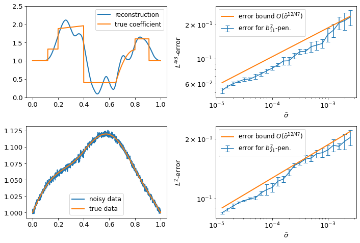
Refer to caption — Figure 1: *Left top:* the true coefficient $c^{\mathrm{jumps}}$ with jumps in the boundary value problem (40) together with the reconstruction for $b^{2}_{{1},{1}}$ -penalization at noise level $\tilde{\sigma}=2.51\cdot 10^{-3}$ . *Left bottom:* Corresponding noisy data together with $F(c^{\mathrm{jumps}})$ . *Right top:* Averaged reconstruction error and its standard derivation using $b^{2}_{{2},{1}}$ -penalization, the rate $\mathcal{O}(\tilde{\sigma}^{1/6})$ in the $L^{2}$ -norm predicted by Theorem 5.1 (see Example 5.9). *Right bottom:* Reconstruction error using $b^{2}_{{1},{1}}$ -penalization, the rate $\mathcal{O}(\tilde{\sigma}^{12/47})$ in the $L^{4/3}$ -norm predicted by Theorem 5.3 (see Example 5.10).

6 Discussion and conclusions

We end this paper by a summary of our results and a comparison to non-oversmoothing regularization theory. Until recently the oversmoothing case in variational regularization theory has been considered more difficult to analyze due to the failure of the tools developed for the non-oversmoothing case so far, which are usually based on some type of source condition. The analysis of this paper, inspired by a series of recent papers discussed in the introduction, suggests that on the contrary oversmoothing may be considered the easier case. The theory is now more complete in many respects than the theory of non-oversmoothing Banach space regularization as the following examples demonstrate:

•

For oversmoothing Banach space regularization, in contrast to the non-oversmoothing case, convergence rate results always remain valid if the norm in the penalty term is replaced by an equivalent norm.
•

So far the analysis of non-oversmoothing Besov space penalization (see [17, 19, 20, 32]) is restricted to certain choices of the Besov norm indices $r$ , $p$ and $q$ and the norm power $u$ , whereas Corollary 3.2 with the generalization in Remark 3.5 only assumes $r>0$ .
•

We are not aware of a convergence rate analysis of BV regularization for the case that the solution belongs to a smoothness class which is smaller than $\mathrm{BV}$ . (The case that the solution smoothness is exactly BV has been analyzed in [9] in a statistical setting.) In contrast, Corollary 4.2 provides optimal convergence rates for BV regularization if the solution only belongs to smoothness classes larger than $\mathrm{BV}$ .

On the other hand, an analysis of exponentially smoothing forward operators and other operators not satisfying a two-sided Lipschitz condition is still missing so far for oversmoothing Banach space regularization. Moreover, more flexibility in the choice of the loss function would be desirable both for the oversmoothing and the non-oversmoothing case, to allow for natural or desirable norms and for comparisons of different methods.

Appendix A Tools from abstract interpolation theory

We first characterize the second part of Assumption 2.2:

Proposition A.1 (Interpolation inequality (see [3, Sec. 3.5, Thm. 3.11.4])).

Suppose ${\mathbb{X}_{\mathcal{R}}}$ , ${\mathbb{X}_{\mathrm{L}}}$ and ${\mathbb{X}_{-}}$ are quasi-Banach spaces with continuous embeddings ${\mathbb{X}_{\mathcal{R}}}\subset{\mathbb{X}_{\mathrm{L}}}\subset{\mathbb{X}_{-}}$ and $\xi\in(0,1).$ Then the following statements are equivalent

1.

${\mathbb{X}_{\mathrm{L}}}$ continuously embeds into $\left({\mathbb{X}_{-}},\mathbb{X}\right)_{\xi,1}$ .

There exists a constant $c>0$ such that

\|f\|_{\mathbb{X}_{\mathrm{L}}}\leq c\|f\|_{\mathbb{X}_{-}}^{1-\xi}\cdot\|f\|_{\mathbb{X}}^{\xi}\quad\text{for all }f\in\mathbb{X}.

Proposition A.2.

Let $\mathbb{X}$ and ${\mathbb{X}_{-}}$ be quasi-Banach spaces with a continuous embedding $\mathbb{X}\subset{\mathbb{X}_{-}}$ . Then have $\mathbb{X}\subset\left({\mathbb{X}_{-}},\mathbb{X}\right)_{1,\infty}$ with embedding constant equal to $1$ .

Proof A.3.

Let $f\in\mathbb{X}$ . Then we insert $h=f$ in the $K$ -functional (3) to obtain

K(t,f)\leq t\|f\|_{\mathbb{X}}\quad\text{ for all }t>0.

Hence $f\in\left({\mathbb{X}_{-}},\mathbb{X}\right)_{1,\infty}$ with $\|f\|_{\left({\mathbb{X}_{-}},\mathbb{X}\right)_{1,\infty}}\leq\|f\|_{\mathbb{X}}$ .

Proposition A.4 (Reiteration).

Let $\mathbb{X}$ and ${\mathbb{X}_{-}}$ be quasi-Banach spaces with a continuous embedding $\mathbb{X}\subset{\mathbb{X}_{-}}$ and let $0<\xi<\theta\leq 1$ . Then

\displaystyle\left({\mathbb{X}_{-}},\mathbb{X}\right)_{\xi,1}=\left({\mathbb{X}_{-}},\left({\mathbb{X}_{-}},\mathbb{X}\right)_{\theta,\infty}\right)_{\frac{\xi}{\theta},1}

with equivalent quasi-norms.

Proof A.5.

In the notation of [3, Def. 3.5.1] we have that ${\mathbb{X}_{-}}$ is of class $\mathcal{C}\left(0,\left({\mathbb{X}_{-}},\mathbb{X}\right)\right)$ . Moreover, $\left({\mathbb{X}_{-}},\mathbb{X}\right)_{\theta,\infty}$ is of class $\mathcal{C}\left(\theta,\left({\mathbb{X}_{-}},\mathbb{X}\right)\right)$ . If $\theta<1$ this is due to [3, Thm. 3.11.4]). For $\theta=1$ the definition yields that $\left({\mathbb{X}_{-}},\mathbb{X}\right)_{1,\infty}$ is of class $\mathcal{C}_{K}\left(1,\left({\mathbb{X}_{-}},\mathbb{X}\right)\right)$ (see [3, Def. 3.5.1]). Moreover, from Proposition A.2 we see

\|f\|_{\left({\mathbb{X}_{-}},\mathbb{X}\right)_{1,\infty}}\leq\|f\|_{\mathbb{X}}\leq t^{-1}\max\{\|f\|_{\mathbb{X}_{-}},t\|f\|_{\mathbb{X}}\}.

Hence $\left({\mathbb{X}_{-}},\mathbb{X}\right)_{1,\infty}$ is of class $\mathcal{C}_{J}\left(1,\left({\mathbb{X}_{-}},\mathbb{X}\right)\right)$ (see again [3, Def. 3.5.1]). Therefore, the result follows from the reiteration theorem [3, Thm. 3.11.5].

Appendix B Properties of Besov spaces

As elsewhere let $\Omega\subset\mathbb{R}^{d}$ be a bounded Lipschitz domain. We first review the relations of Besov spaces to $L^{p}$ -spaces and to the Sobolev spaces $W^{s}_{p}(\Omega)$ , $s\geq 0$ , $p\in(1,\infty)$ . Recall that for $s\in\mathbb{N}_{0}$ Sobolev norms are given by $\|f\|_{W^{s}_{p}}^{p}=\sum_{\alpha\in\mathbb{N}_{0}^{d},|\alpha|\leq s}\|D^{\alpha}f\|_{L^{p}}^{p}$ . For non-integer $s$ these spaces are also called Sobolev-Slobodeckij spaces, and for $p=2$ they coincide with the $H^{s}_{2}(\Omega)$ spaces defined on $\mathbb{R}^{d}$ via Fourier transform for all $s\in\mathbb{R}$ .

Proposition B.1 (Embeddings with $L^{p}$ and Sobolev spaces).

1.

Let $p\in(1,\infty)$ . Then we have continuous embeddings

(41) $\displaystyle B^{0}_{{p},{\min\{p,2\}}}(\Omega)\subset L^{p}(\Omega)\subset B^{0}_{{p},{\max\{p,2\}}}(\Omega).$

For $p=1$ the following continuous embeddings hold true:

(42) $\displaystyle B^{0}_{{1},{1}}(\Omega)\subset L^{1}(\Omega)\subset B^{0}_{{1},{\infty}}(\Omega).$
2.

$B^{s}_{{p},{p}}(\Omega)=W^{s}_{p}(\Omega)$ with equivalent norms for all $0<s\notin\mathbb{N}$ and $p\in(1,\infty)$ , and in case of $p=2$ for all $s\in\mathbb{R}$ .

Let $p_{0},p_{1},q_{0},q_{1}\in(0,\infty]$ and $-\infty<s_{1}<s_{0}<\infty$ . Then

(43)

\displaystyle B^{s_{0}}_{{p_{0}},{q_{0}}}(\Omega)\subset B^{s_{1}}_{{p_{1}},{q_{0}}}(\Omega)\quad\mbox{if}\quad s_{0}-\frac{d}{p_{0}}=s_{1}-\frac{d}{p_{1}}

and

(44)

\displaystyle B^{s_{0}}_{{p_{0}},{q_{0}}}(\Omega)\subset B^{s_{1}}_{{p_{1}},{q_{1}}}(\Omega)\quad\mbox{if}\quad s_{0}-\frac{d}{p_{0}}>s_{1}-\frac{d}{p_{1}}.

4.

Let $s\in\mathbb{R}$ and $p,q_{0},q_{1}\in(0,\infty]$ . Then

(45) $\displaystyle B^{s}_{{p},{q_{0}}}(\Omega)\subset B^{s}_{{p},{q_{1}}}(\Omega)\quad\mbox{if}\quad q_{0}\leq q_{1}$

Proof B.2.

First note that as all occurring spaces on bounded Lipschitz domains in $\mathbb{R}^{d}$ are defined by restriction of the respective spaces on $\mathbb{R}^{d}$ it suffices to prove the assertions for $\Omega=\mathbb{R}^{d}$ .

Let $F^{s}_{p,q}(\Omega)$ be the function spaces defined in [30, 2.3.1. Def. 2(ii)] for $\Omega=\mathbb{R}^{d}$ . By [30, 3.2.4.(3)] we have continuous embeddings

(46)

\displaystyle B^{s}_{{p},{\min\{p,q\}}}(\Omega)\subset F^{s}_{p,q}(\Omega)\subset B^{s}_{{p},{\max\{p,q\}}}(\Omega)\quad\text{for all}\quad p,q\in[1,\infty).

With this the embeddings for $p>1$ follow from the identity $F^{0}_{p,2}(\Omega)=L^{p}(\Omega)$ with equivalent norms. The latter identity can be found in [30, 2.5.6.]. For the assertion in the case $p=1$ we refer to [30, 2.5.7.(2)].

2.

See [27, §2.3 and Thm. 4.2.4].
3.

See [30, Prop. 3.3.1].
4.

The inclusion for $\Omega$ replaced by $\mathbb{R}^{d}$ can be found in [30, eq. (2.3.2/5)]. Using the definition of the $B^{s}_{{p},{q}}(\Omega)$ spaces, this easily implies the assertion.

We now recall some well-known results on interpolation of Besov spaces. Besides $K$ -interpolation reviewed in Section 2.1 we also refer to the complex interpolation method in some remarks. The latter only works for complex Banach spaces $X_{0},X_{1}$ as well as some some quasi-Banach spaces, and it is denoted by $[X_{0},X_{1}]_{\theta}=X_{\theta}$ for $\theta\in(0,1)$ (see [3]).

Proposition B.3 (interpolation of Besov spaces).

Let $s_{0},s_{1}\in\mathbb{R}$ , $s_{0}\neq s_{1}$ , $\theta\in(0,1)$ , and $s_{\theta}:=(1-\theta)s_{0}+\theta s_{1}$ .

1.

For $p,q_{0},q_{1}\in(0,\infty]$ and $q\in[1,\infty]$ we have

(47) $\displaystyle\left(B^{s_{0}}_{{p},{q_{0}}}(\Omega),B^{s_{1}}_{{p},{q_{1}}}(\Omega)\right)_{\theta,q}=B^{s_{\theta}}_{{p},{q}}(\Omega).$

If $p_{0},p_{1},p_{\theta}\in(0,\infty)$ with $\frac{1}{p_{\theta}}=\frac{1-\theta}{p_{0}}+\frac{\theta}{p_{1}}$ , then

(48)

\displaystyle\left(B^{s_{0}}_{{p_{0}},{p_{0}}}(\Omega),B^{s_{1}}_{{p_{1}},{p_{1}}}(\Omega)\right)_{\theta,p_{\theta}}=B^{s_{\theta}}_{{p_{\theta}},{p_{\theta}}}(\Omega).

If $p_{0},p_{1},p_{\theta}\in[1,\infty)$ with $\frac{1}{p_{\theta}}=\frac{1-\theta}{p_{0}}+\frac{\theta}{p_{1}}$ and $q_{0},q_{\theta},q_{1}\in[1,\infty)$ , with $\frac{1}{q_{\theta}}=\frac{1-\theta}{q_{0}}+\frac{\theta}{q_{1}}$ , then

(49)

\displaystyle\left[B^{s_{0}}_{{p_{0}},{q_{0}}}(\Omega),B^{s_{1}}_{{p_{1}},{q_{1}}}(\Omega)\right]_{\theta}=B^{s_{\theta}}_{{p_{\theta}},{q_{\theta}}}(\Omega).

Proof B.4.

See [30, Thm. 3.3.6] for the first and last statement and [30, Thm. 2.4.3 and Remark 8 in §3.3.6] for the second statement.

Appendix C On spaces of functions of bounded variation

Finally, we also recall and generalize some results on functions of bounded variation.

Proposition C.1 (Embedding).

Let $a\geq 0$ with $a\geq\frac{d}{2}-1$ . Then there is a continuous embedding $\mathrm{BV}(\Omega)\subset B^{-a}_{{2},{2}}(\Omega)$ .

Proof C.2.

For all embeddings involving the space $\mathrm{BV}(\Omega)$ in this proof we refer to [2, Cor. 3.49 & Prop. 3.21]. For $d=1$ there is a continuous embedding $\mathrm{BV}(\Omega)\subset L^{2}(\Omega)$ . We have $L^{2}(\Omega)=B^{0}_{{2},{2}}(\Omega)\subset B^{-a}_{{2},{2}}(\Omega)$ , which yields the claim in this case.
For $d>1$ we set $p:=\frac{d}{d-1}$ . Then $p\in(1,2]$ and there is a continuous embedding $\mathrm{BV}(\Omega)\subset L^{p}(\Omega)$ . By Proposition B.1 we have a continuous embedding $L^{p}(\Omega)\subset B^{0}_{{p},{2}}(\Omega)$ . Furthermore, $a+\frac{d}{2}\geq d-1=\frac{d}{p}$ yields a continuous embedding $B^{0}_{{p},{2}}(\Omega)\subset B^{-a}_{{2},{2}}(\Omega)$ . Putting together the latter three embeddings yields the claim.

Proposition C.3.

Let $a\geq 0$ , $s\in(-a,1)$ , and $\Omega\subset\mathbb{R}^{d}$ a bounded Lipschitz domain. Then

\displaystyle B^{s}_{{t_{s}},{t_{s}}}(\Omega)=\left(B^{-a}_{{2},{2}}(\Omega),\mathrm{BV}(\Omega)\right)_{\theta_{s},t_{s}}\quad\text{ with }\theta_{s}:=\frac{s+a}{a+1}\text{ and }t_{s}:=\frac{2a+2}{s+2a+1}

with equivalent norms.

Proof C.4.

First note that if $f\in\mathrm{BV}(\mathbb{R}^{d})$ , then

f|_{\Omega}\in\mathrm{BV}(\Omega)\quad\text{with}\quad\|f|_{\Omega}\|_{\mathrm{BV}(\Omega)}\leq\|f\|_{\mathrm{BV}(\mathbb{R}^{d})}.

Due to [6, Thm. 1.4] to claim holds true for $\Omega=\mathbb{R}^{d}$ . Note that here the condition $\gamma<1-\frac{1}{d}$ from the latter reference on $\gamma:=\frac{-(2a+2)}{d}+1$ is satisfied. Let $c_{1}$ be a constant such that the norm in $B^{s}_{{t_{s}},{t_{s}}}(\mathbb{R}^{d})$ is bounded by $c_{1}$ times the norm in $\left(B^{-a}_{{2},{2}}(\mathbb{R}^{d}),\mathrm{BV}(\mathbb{R}^{d})\right)_{\theta_{s},t_{s}}$ and the other way around.
We transfer this result to bounded Lipschitz domains. To this end we separately prove both inclusions in the stated identity.
Let $f\in B^{s}_{{t_{s}},{t_{s}}}(\Omega)$ . Then there exists $\tilde{f}\in B^{s}_{{t_{s}},{t_{s}}}(\mathbb{R}^{d})$ with

\tilde{f}|_{\Omega}=f\quad\text{and}\quad\|\tilde{f}\|_{B^{s}_{{t_{s}},{t_{s}}}(\mathbb{R}^{d})}\leq 2\|f\|_{B^{s}_{{t_{s}},{t_{s}}}(\Omega)}.

Let $t>0$ and $\tilde{f}=\tilde{f}_{1}+\tilde{f}_{2}$ with $\tilde{f}_{1}\in B^{-a}_{{2},{2}}(\mathbb{R}^{d})$ and $\tilde{f}_{2}\in\mathrm{BV}(\mathbb{R}^{d})$ be a decomposition such that

\|\tilde{f}_{1}\|_{B^{-a}_{{2},{2}}(\mathbb{R}^{d})}+t\|\tilde{f}_{2}\|_{\mathrm{BV}(\mathbb{R}^{d})}\leq 2K(t,\tilde{f})

with the $K$ -functional from real interpolation of Banach spaces. Then $\tilde{f}_{1}|_{\Omega}\in B^{-a}_{{2},{2}}(\Omega)$ , $\tilde{f}_{2}|_{\Omega}\in\mathrm{BV}(\Omega)$ , $f=f_{1}+f_{2}$ and

K(t,f)\leq\|\tilde{f}_{1}|_{\Omega}\|_{B^{-a}_{{2},{2}}(\Omega)}+t\|\tilde{f}_{2}|_{\Omega}\|_{\mathrm{BV}(\Omega)}\leq 2K(t,\tilde{f}).

Hence with the definition of the norm on real interpolation spaces we obtain

\|f\|_{\left(B^{-a}_{{2},{2}}(\Omega),\mathrm{BV}(\Omega)\right)_{\theta_{s},t_{s}}}\!\!\!\leq 2\|\tilde{f}\|_{\left(B^{-a}_{{2},{2}}(\mathbb{R}^{d}),\mathrm{BV}(\mathbb{R}^{d})\right)_{\theta_{s},t_{s}}}\!\!\!\leq 2c_{1}\|\tilde{f}\|_{B^{s}_{{t_{s}},{t_{s}}}(\mathbb{R}^{d})}\leq 4c_{1}\|f\|_{B^{s}_{{t_{s}},{t_{s}}}(\Omega)}.

We turn to the other inclusion. There exists a constant $C_{\mathrm{ext}}>0$ such that for every ${f\in B^{-a}_{{2},{2}}(\Omega)}$ there exists $\tilde{f}\in B^{-a}_{{2},{2}}(\mathbb{R}^{d})$ with $\tilde{f}|_{\Omega}=f$ and $\|\tilde{f}\|_{B^{-a}_{{2},{2}}(\mathbb{R}^{d})}\leq C_{\mathrm{ext}}\|f\|_{B^{-a}_{{2},{2}}(\Omega)}$ and likewise for every $f\in\mathrm{BV}(\Omega)$ there exists $\tilde{f}\in\mathrm{BV}(\mathbb{R}^{d})$ with

\tilde{f}|_{\Omega}=f\quad\text{and}\quad\|\tilde{f}\|_{\mathrm{BV}(\mathbb{R}^{d})}\leq C_{\mathrm{ext}}\|f\|_{\mathrm{BV}(\Omega)}.

This holds true by the definition of $B^{-a}_{{2},{2}}(\Omega)$ via restrictions and due to [2, Prop. 3.21] for of bounded variation functions. Now suppose $f\in\left(B^{-a}_{{2},{2}}(\Omega),\mathrm{BV}(\Omega)\right)_{\theta_{s},t_{s}}$ . Let $f=f_{1}+f_{2}$ with $f_{1}\in B^{-a}_{{2},{2}}(\Omega)$ and $f_{2}\in\mathrm{BV}(\Omega)$ such that

\|f_{1}\|_{B^{-a}_{{2},{2}}(\Omega)}+t\|f_{2}\|_{\mathrm{BV}(\Omega)}\leq 2K(t,f).

Let $\tilde{f}_{1}\in B^{-a}_{{2},{2}}(\mathbb{R}^{d})$ and $\tilde{f}_{2}\in\mathrm{BV}(\mathbb{R}^{d})$ be extensions as above. Then $\tilde{f}:=\tilde{f}_{1}+\tilde{f}_{2}$ satisfies $\tilde{f}|_{\Omega}=f$ , and

K(t,\tilde{f}_{1}+\tilde{f}_{2})\leq\|\tilde{f}_{1}\|_{B^{-a}_{{2},{2}}(\mathbb{R}^{d})}+t\|\tilde{f}_{2}\|_{\mathrm{BV}(\mathbb{R}^{d})}\leq 2C_{e}K(t,f).

We conclude that

	$\displaystyle\\|f\\|_{B^{s}_{{t_{s}},{t_{s}}}(\Omega)}$	$\displaystyle\leq\\|\tilde{f}\\|_{B^{s}_{{t_{s}},{t_{s}}}(\mathbb{R}^{d})}\leq c_{1}\\|\tilde{f}\\|_{\left(B^{-a}_{{2},{2}}(\mathbb{R}^{d}),\mathrm{BV}(\mathbb{R}^{d})\right)_{\theta_{s},t_{s}}}$
		$\displaystyle\leq 2c_{1}C_{e}\\|f\\|_{\left(B^{-a}_{{2},{2}}(\Omega),\mathrm{BV}(\Omega)\right)_{\theta_{s},t_{s}}}.$

References

[1] R. Acar and C. R. Vogel. Analysis of bounded variation penalty methods for ill-posed problems. Inverse problems, 10(6):1217, 1994.
[2] L. Ambrosio, N. Fusco, and D. Pallara. Functions of bounded variation and free discontinuity problems. Oxford Mathematical Monographs, The Clarendon Press Oxford University Press, New York, 2000.
[3] J. Bergh and J. Löfström. Interpolation spaces. Springer Berlin Heidelberg, 1976.
[4] K. Bredies and D. A. Lorenz. Regularization with non-convex separable constraints. Inverse Problems, 25(8):085011, 2009.
[5] D.-H. Chen, B. Hofmann, and I. Yousept. Oversmooting Tikhonov regularization in Banach spaces. Inverse Problems, to appear.
[6] A. Cohen, W. Dahmen, I. Daubechies, R. DeVore, et al. Harmonic analysis of the space bv. Revista Matematica Iberoamericana, 19(1):235–263, 2003.
[7] M. del Álamo. Multiscale Total Variation Estimators for Regression and Inverse Problems. PhD thesis, Georg-August University, 2019.
[8] M. del Álamo, H. Li, and A. Munk. Frame-constrained total variation regularization for white noise regression. The Annals of Statistics, 49(3):1318–1346, 2021.
[9] M. del Álamo and A. Munk. Total variation multiscale estimators for linear inverse problems. Inf. Inference, 9(4):961–986, 2020.
[10] D. Donoho and I. M. Johnstone. Minimax estimation via wavelet shrinkage. Ann. Statist., 26:879–921, 1998.
[11] H. W. Engl, M. Hanke, and A. Neubauer. Regularization of inverse problems, volume 375 of Mathematics and its Applications. Kluwer Academic Publishers Group, Dordrecht, 1996.
[12] D. Freitag. Real interpolation of weighted $l^{p}$ -spaces. Mathematische Nachrichten, 86(1):15–18, 1978.
[13] D. Gerth and B. Hofmann. Oversmoothing regularization with $\ell^{1}$ -penalty term. AIMS Math., 4(4):1223–1247, 2019.
[14] E. Giné and R. Nickl. Mathematical foundations of infinite-dimensional statistical models, volume 40. Cambridge University Press, 2015.
[15] B. Hofmann and P. Mathé. Tikhonov regularization with oversmoothing penalty for non-linear ill-posed problems in Hilbert scales. Inverse Problems, 34(1):015007, dec 2018.
[16] B. Hofmann and R. Plato. Convergence results and low order rates for nonlinear Tikhonov regularization with oversmoothing penalty term. Electron. Trans. Numer. Anal., 53:313–328, 2020.
[17] T. Hohage and P. Miller. Optimal convergence rates for sparsity promoting wavelet-regularization in Besov spaces. Inverse Problems, 35:65005 (27pp), 2019.
[18] E. Mammen and S. van de Geer. Locally adaptive regression splines. Ann. Statist., 25(1):387–413, 1997.
[19] P. Miller. Variational regularization theory based on image space approximation rates. Inverse Problems, 37(6):065003, May 2021.
[20] P. Miller and T. Hohage. Maximal spaces for approximation rates in $\ell^{1}$ -regularization. Numerische Mathematik, pages 1–34, 2021.
[21] F. Natterer. Error bounds for Tikhonov regularization in Hilbert scales. Applicable Anal., 18:29–37, 1984.
[22] A. Rastogi. Tikhonov regularization with oversmoothing penalty for nonlinear statistical inverse problems. Technical report, arXiv:2002.01303, 2020.
[23] O. Scherzer, M. Grasmair, H. Grossauer, M. Haltmeier, and F. Lenzen. Variational methods in imaging, volume 167 of Applied Mathematical Sciences. Springer, New York, 2009.
[24] T. Schuster, B. Kaltenbacher, B. Hofmann, and K. S. Kazimierski. Regularization methods in Banach spaces. De Gruyter, July 2012.
[25] I. W. Selesnick and I. Bayram. Sparse signal estimation by maximally sparse convex optimization. IEEE Transactions on Signal Processing, 62(5):1078–1092, 2014.
[26] A. N. Tikhonov. On the solution of incorrectly formulated problems and the regularization method. Soviet Math. Doklady, 4:1035–1038, 1963. Englisch translation.
[27] H. Triebel. Interpolation theory, function spaces, differential operators. VEB Deutscher Verlag der Wissenschaften, Berlin, 1978.
[28] H. Triebel. Theory of function spaces II. Modern Birkhäuser Classics. Springer, Basel, 1992.
[29] H. Triebel. Function spaces and wavelets on domains, volume 7 of EMS Tracts in Mathematics. European Mathematical Society (EMS), Zürich, 2008.
[30] H. Triebel. Theory of function spaces. Modern Birkhäuser Classics. Springer, Basel, reprint. edition, 2010. Reprint of the 1983 edition.
[31] M. C. Veraar. Regularity of Gaussian white noise on the $d$ -dimensional torus. Banach Center Publications, 95:385–398, 2011.
[32] F. Weidling, B. Sprung, and T. Hohage. Optimal convergence rates for Tikhonov regularization in Besov spaces. SIAM J. Numer. Anal., 58:21–47, 2020.
[33] C. A. Zarzer. On tikhonov regularization with non-convex sparsity constraints. Inverse Problems, 25(2):025006, 2009.

	$\displaystyle\frac{1}{2\alpha}\\|F(f)-F(f_{\alpha})\\|_{\mathbb{Y}}^{2}+\frac{1}{u}\\|f_{\alpha}\\|_{\mathbb{X}_{\mathcal{R}}}^{u}$	$\displaystyle\leq\frac{1}{2\alpha}\\|F(f)-F(f_{t})\\|_{\mathbb{Y}}^{2}+\frac{1}{u}\\|f_{t}\\|_{\mathbb{X}_{\mathcal{R}}}^{u}$
		$\displaystyle\leq\frac{M_{2}^{2}}{2\alpha}\\|f-f_{t}\\|_{\mathbb{X}_{-}}^{2}+\frac{1}{u}\\|f_{t}\\|_{\mathbb{X}_{\mathcal{R}}}^{u}$
		$\displaystyle\leq\frac{2M_{2}^{2}}{\alpha}\varrho^{2}t^{2\theta}+\frac{2^{u}}{u}\varrho^{u}t^{(\theta-1)u}$
		$\displaystyle=c_{1}\varrho^{\frac{2u}{(1-\theta)u+2\theta}}\alpha^{\frac{(\theta-1)u}{(1-\theta)u+2\theta}}$

	$\displaystyle\frac{1}{2\alpha}\\|g^{\mathrm{obs}}-F(\hat{f}_{\alpha})\\|_{\mathbb{Y}}^{2}$	$\displaystyle+\frac{1}{u}\\|\hat{f}_{\alpha}\\|_{\mathbb{X}_{\mathcal{R}}}^{u}\leq$
		$\displaystyle\leq\frac{1}{2\alpha}\\|g^{\mathrm{obs}}-F(f)+F(f)-F(f_{t})\\|_{\mathbb{Y}}^{2}+\frac{1}{u}\\|f_{t}\\|_{\mathbb{X}_{\mathcal{R}}}^{u}$
		$\displaystyle\leq\frac{\delta^{2}}{\alpha}+\frac{M_{2}^{2}}{\alpha}\\|f-f_{t}\\|_{\mathbb{X}_{-}}^{2}+\frac{2^{u}}{u}\varrho^{u}t^{(\theta-1)u}$
		$\displaystyle\leq(1+4M_{2}^{2}C_{L}^{-\frac{2\theta}{\theta-\xi}})\frac{\delta^{2}}{\alpha}+\frac{2^{u}}{u}C_{L}^{\frac{(1-\theta)u}{\theta-\xi}}\varrho^{\frac{u}{\theta}}\delta^{\frac{(\theta-1)u}{\theta}}$
		$\displaystyle\leq c_{5}\varrho^{\frac{u}{\theta}}\delta^{\frac{(\theta-1)u}{\theta}}$

	$\displaystyle\\|g^{\mathrm{obs}}-F(f_{t})\\|_{\mathbb{Y}}^{2}$	$\displaystyle\leq(1+\varepsilon)\delta^{2}+(1+\varepsilon^{-1})\\|F(f)-F(f_{t})\\|_{\mathbb{Y}}^{2}$
		$\displaystyle\leq(1+\varepsilon)\delta^{2}+(1+\varepsilon^{-1})M_{2}\\|f-f_{t}\\|_{\mathbb{X}_{-}}^{2}$
		$\displaystyle\leq(1+2\varepsilon)\delta^{2}\leq c_{\mathrm{D}}^{2}\delta^{2}\leq\\|g^{\mathrm{obs}}-F(\hat{f}_{\alpha})\\|_{\mathbb{Y}}^{2}.$

	$\displaystyle\frac{1}{2\alpha}\\|g_{t}-\hat{g}_{\alpha}\\|_{\mathbb{Y}}^{2}+\frac{1}{u}\\|\hat{f}_{\alpha}\\|^{u}_{\mathbb{X}_{\mathcal{R}}}$
(31)		$\displaystyle\leq\frac{1}{2\alpha}\\|g_{t}-\hat{g}_{\alpha}\\|_{\mathbb{Y}}^{2}+\frac{1}{\alpha}\mathcal{S}_{g^{\mathrm{obs}}}(g_{t})-\frac{1}{\alpha}\mathcal{S}_{g^{\mathrm{obs}}}(\hat{g}_{\alpha})+\frac{1}{u}\\|f_{t}\\|_{{}_{\mathbb{X}_{\mathcal{R}}}}^{u}$
	$\displaystyle=\frac{1}{\alpha}\left\langle\sigma Z,\hat{g}_{\alpha}-g_{t}\right\rangle+\frac{1}{\alpha}\left\langle F(f)-g_{t},\hat{g}_{\alpha}-g_{t}\right\rangle+\frac{1}{u}\\|f_{t}\\|_{{}_{\mathbb{X}_{\mathcal{R}}}}^{u}.$

	$\displaystyle\frac{1}{\alpha}\left\langle\sigma Z,\hat{g}_{\alpha}-g_{t}\right\rangle$	$\displaystyle\leq\frac{1}{\alpha}\\|\sigma Z\\|_{B^{-d/2}_{p^{\prime},\infty}}\left\\|g_{t}-\hat{g}_{\alpha}\right\\|_{B_{p,1}^{d/2}}$
		$\displaystyle\leq c_{1}\frac{\sigma N}{\alpha}\left\\|g_{t}-\hat{g}_{\alpha}\right\\|_{B^{0}_{p,2}}^{1-\frac{d}{2a+2r}}\left\\|g_{t}-\hat{g}_{\alpha}\right\\|_{B_{p,q}^{a+r}}^{\frac{d}{2a+2r}}$
(33)			$\displaystyle\leq c_{2}\frac{\sigma N}{\alpha}\left\\|g_{t}-\hat{g}_{\alpha}\right\\|_{\mathbb{Y}}^{1-\frac{d}{2a+2r}}\left\\|f_{t}-\hat{f}_{\alpha}\right\\|_{{\mathbb{X}_{\mathcal{R}}}}^{\frac{d}{2a+2r}}$
		$\displaystyle=\left(c_{2}\sigma N\alpha^{-\frac{a+r+d/2}{2a+2r}}\right)\left(\frac{1}{\alpha}{\left\\|g_{t}-\hat{g}_{\alpha}\right\\|_{\mathbb{Y}}^{2}}\right)^{\frac{a+r-d/2}{2a+2r}}\left(\left\\|f_{t}-\hat{f}_{\alpha}\right\\|_{{\mathbb{X}_{\mathcal{R}}}}^{u}\right)^{\frac{d}{u(2a+2r)}}$