Stochastic hydrodynamics and hydro-kinetics: Similarities and differences

Experimental facilities such as the Relativistic Heavy-Ion Collider (RHIC) and the Large Hadron Collider (LHC) collide nuclei at high energies to study and quantify properties of the quark-gluon plasma. Relativistic hydrodynamics provides a macroscopic and quantitative description of the fireball evolution in heavy-ion collisions Heinz and Snellings 2013; Gale et al. 2013; Shen and Yan 2020. The applicability of hydrodynamics is justified if the mean free paths of the particles are small compared to the distances over which thermodynamic quantities vary. It has been successfully used to constrain various transport properties of the quark-gluon plasma such as specific shear and bulk viscosity and thermal conductivity Pratt et al. 2015; Bernhard et al. 2016; Bernhard et al. 2019; Everett et al. 2021a; Everett et al. 2021b; Nijs et al. 2021a; Nijs et al. 2021b. Hybrid frameworks that combine hydrodynamics with a hadronic transport model can reproduce various flow measurements with successful predictive power Song et al. 2011; Shen et al. 2016; Putschke et al. 2019; Schenke et al. 2020.

Relativistic hydrodynamics involves differential equations for the energy-momentum tensor and the charge currents. Ripples caused by stochastic thermal fluctuations will give corrections to macroscopic variables of hydrodynamics Young et al. 2015. The fluctuation-dissipation theorem Kapusta et al. 2012 relates dissipative properties to the amplitude of hydrodynamic fluctuations. Hence, study of fluctuations can be leveraged to study quark-gluon plasma transport properties Pratt and Young 2017; Pratt and Plumberg 2019. Specifically, fluctuations are known to become important near critical points Plumberg and Kapusta 2017; Bzdak et al. 2020; Bluhm et al. 2020; An et al. 2022. This has led to studies that investigate fluctuations in conserved quantities, such as electric charge, baryon number, and strangeness on an event-by-event basis Kapusta and Plumberg 2018; Pratt et al. 2018; Pratt and Plumberg 2020; De et al. 2020. Recently, there have also been studies of dynamic critical phenomena near a QCD critical point Nahrgang and Bluhm 2020; Rajagopal et al. 2020; Du et al. 2020; An et al. 2022; Du et al. 2021. Non-Gaussianities (higher-order cumulants) also become important near critical points as they are more sensitive to large correlation lengths Bzdak et al. 2020.

It is important to systematically study fluctuations in heavy-ion collision systems. Adding noise to hydrodynamic equations transforms the hydrodynamical equations from partial differential equations to stochastic differential equations. Historically, stochastic differential equations have been notorious to deal with Young et al. 2015; Murase 2015; Singh et al. 2019; Sakai et al. 2020; Sakai et al. 2021. Broadly, there have been two methods to study the effect of fluctuations. The first is the direct method of studying stochastic differential equations through analytical and numerical techniques Kapusta and Plumberg 2018; Young et al. 2015; Singh et al. 2019; Sakai et al. 2020; Pratt et al. 2018; Pratt and Plumberg 2020; De et al. 2020. One can simulate stochastic differential equations like usual partial differential equations over millions of different realizations of the noise. Statistical properties of those solutions are studied to understand the underlying physical process. Alternatively, some authors have suggested the use of a set of deterministic kinetic equations to capture the behavior of time evolution of $n$-point correlations of hydrodynamic variables Akamatsu et al. 2017; Stephanov and Yin 2018; Akamatsu et al. 2019; An et al. 2019; Martinez et al. 2019; An et al. 2020; Martinez and Schäfer 2017. This approach has come to be known as the hydro-kinetic approach. The method relies on the truncation of higher moments from noisy hydrodynamic calculations and holds the advantage over direct numerical studies of SDEs by being computationally less intensive.

It seems imperative that a direct comparison between the hydro-kinetic approach and the stochastic hydro formalism needs to be made which is lacking in the current literature. In this paper, we compare the two approaches for a system with just one conserved charge in an expanding fluid background, namely the Bjorken system Bjorken 1983. At the top RHIC and LHC energies, the charge current decouples from the energy-momentum conservation because the net charge is small and therefore can be studied separately. The system with a single conserved charge is simple enough to allow for analytical calculations. Additionally, the conserved baryon density is believed to be an order parameter for a possible critical point in the QCD phase diagram Bzdak et al. 2020. The usual diffusion equation has an infinite signal propagation speed. To make it finite, we also study the Catteneo equation and which introduces so-called colored noise in the hydrodynamical equations Kapusta and Young 2014a; Kapusta and Young 2014b. In the presence of colored noise, the hydrodynamics become causal. We show the comparison of hydro-kinetics to causal hydrodynamics as well.

The paper is organized as follows. We give a concise description of the dynamical evolution of one conserved charge in a 1+1D Bjorken system in Sec. II. In Sec. III, we derive the hydro-kinetic equations and compare them with the stochastic calculation in the white noise limit. We extend the comparison for the colored noise case to hydro-kinetics in Sec. IV. Sec. V summarizes our concluding remarks. Complementary calculations without transverse dynamics are provided in the Appendix A.

The assumption of longitudinal boost invariance implies that the initial conditions for local variables are functions of the proper time $\tau\equiv\sqrt{t^{2}-z^{2}}$ and the transverse coordinates $x$ and $y$. They do not depend on spacetime rapidity $\xi\equiv\tanh^{-1}\left(z/t\right)$. We define fluid velocity $u^{\mu}$ to be the velocity of the energy-momentum current, known as the Landau-Lifshitz frame,

$$T^{\mu\nu}u_{\nu}=eu^{\mu}.$$

(1)

We consider a single species of conserved charge in the fluid. This charge current takes the form

$$J^{\mu}=n_{Q}u^{\mu}+\Delta J^{\mu}+I^{\mu},$$

(2)

where $n_{Q}$ is the charge density in the local rest frame of the fluid cell, $\Delta J^{\mu}$ is the diffusion current, and $I^{\mu}$ is the noise current. The fluctuation-dissipation theorem dictates that dissipation is always accompanied by stochastic noises for any equilibrium system. In the conventional, lowest order in derivatives diffusion equation, $\Delta J^{\mu}$ takes the form

$$\Delta J^{\mu}=D_{Q}\nabla^{\mu}n_{Q}=\sigma_{Q}\,T\,\nabla^{\mu}\left(\frac{\mu_{Q}}{T}\right),$$

(3)

where $\mu_{Q}$ is the charge chemical potential, $\sigma_{Q}$ is the charge conductivity, and $\nabla^{\mu}$ is the transverse derivative

$$\nabla^{\mu}\equiv\Delta^{\mu\nu}\partial_{\nu}=\partial^{\mu}-u^{\mu}(u\cdot\partial)$$

(4)

with the projection operator $\Delta^{\mu\nu}=g^{\mu\nu}-u^{\mu}u^{\nu}$. One can verify that the charge current conservation equation $\partial_{\mu}J^{\mu}=0$ in the local rest frame where $u^{\mu}=(1,\mbox{\boldmath$0$})$ follows the usual diffusion equation

$$\left(\frac{\partial}{\partial t}-D_{Q}\nabla^{2}\right)n_{Q}=0\,.$$

(5)

The diffusion constant $D_{Q}$ and charge conductivity are related by the Einstein relation $D_{Q}=\sigma_{Q}/\chi_{Q}$, where $\chi_{Q}$ is the electric charge susceptibility defined by

$$\chi_{Q}=\frac{\partial n_{Q}(T,\mu_{Q})}{\partial\mu_{Q}}\,.$$

(6)

Following Refs. Kapusta and Plumberg 2018; De et al. 2020, we assume $\chi_{Q}\propto T^{2}$. The amplitudes for dissipation and stochastic noise are related by the fluctuation-dissipation theorem which is justified because the fluid description assumes the system is close to local equilibrium. In other words, modes disturbed by $I^{\mu}$ are equilibrated by the viscous term $\Delta J^{\mu}$. The 1-point function of the noise $\langle I^{\mu}\rangle$ vanishes while the 2-point functions are determined by the fluctuation-dissipation theorem. Assuming white noise

$$\langle I^{\mu}(x)\rangle=0,\quad\langle I^{\mu}(x_{1})I^{\nu}(x_{2})\rangle=2\sigma_{Q}T\,\Delta^{\mu\nu}\delta(x_{1}-x_{2}).$$

(7)

Such a noise function whose 2-point correlation is proportional to the Dirac $\delta$-function in both space and time is referred to as white noise.

We adopt Milne coordinates which are proper time and space-time rapidity,

$\displaystyle\begin{aligned} t&=&\tau\cosh\xi\qquad z&=\tau\sinh\xi\\ \tau&=&\sqrt{t^{2}-z^{2}}\qquad\xi&=\tanh^{-1}\left(\frac{z}{t}\right).\\ \end{aligned}$

(8)

The transverse coordinates $x$ and $y$ are the same as in Cartesian coordinates. The non-zero components of the background flow velocity are

$$u^{0}=\cosh\xi\qquad u^{z}=\sinh\xi\,.$$

(9)

The transverse derivatives in the $t$ and $z$ directions are

$\displaystyle\nabla^{0}=-\frac{\sinh\xi}{\tau}\frac{\partial}{\partial\xi}\qquad\nabla^{3}=-\frac{\cosh\xi}{\tau}\frac{\partial}{\partial\xi}$

(10)

with $\,u\cdot\partial=\partial/\partial\tau$. The entropy density $s$ can be factored out from the noise current $I^{\mu}$ so as to capture the fluctuating part in the random dimensionless scalars $f$, $g_{1}$ and $g_{2}$.

	$\displaystyle I^{t}$	$\displaystyle=$	$\displaystyle s(\tau)\;f(\xi,\tau,x,y)\sinh\xi$
	$\displaystyle I^{z}$	$\displaystyle=$	$\displaystyle s(\tau)\;f(\xi,\tau,x,y)\cosh\xi$
	$\displaystyle I^{x}$	$\displaystyle=$	$\displaystyle s(\tau)\;g_{1}(\xi,\tau,x,y)$
	$\displaystyle I^{y}$	$\displaystyle=$	$\displaystyle s(\tau)\;g_{2}(\xi,\tau,x,y)$		(11)

Here $f,g_{1},g_{2}$ are uncorrelated random scalar functions with the following 2-point correlation in Cartesian coordinates

	$\displaystyle\langle f(x_{1})f(x_{2})\rangle$	$\displaystyle=$	$\displaystyle\langle g_{1}(x_{1})g_{1}(x_{2})\rangle=\langle g_{2}(x_{1})g_{2}(x_{2})\rangle$		(12)
		$\displaystyle=$	$\displaystyle\frac{2\sigma_{Q}T}{s^{2}}\delta^{4}(x_{1}-x_{2})\;\;\;$

and

$$\langle f(x_{1})g_{1}(x_{2})\rangle=\langle g_{2}(x_{1})g_{1}(x_{2})\rangle=\langle f(x_{1})g_{2}(x_{2})\rangle=0.$$

(13)

The last equation denotes that the random functions $f$, $g_{1}$ and $g_{2}$ are uncorrelated with each other.

The background conservation equations for the charge density and entropy density are

	$\displaystyle\frac{ds}{d\tau}+\frac{s}{\tau}=0\;\;$	$\displaystyle\Rightarrow$	$\displaystyle\;\;s(\tau)=\frac{s_{i}\tau_{i}}{\tau}$		(14)
	$\displaystyle\frac{dn_{Q}}{d\tau}+\frac{n_{Q}}{\tau}=0\;\;$	$\displaystyle\Rightarrow$	$\displaystyle\;\;n_{Q}(\tau)=\frac{n_{i}\tau_{i}}{\tau}\,.$		(15)

The $s_{i}$ and $n_{i}$ are the entropy and charge densities at some initial time $\tau_{i}$. We take the initial charge density $n_{i}$ to be zero, hence the average charge density for subsequent times is zero as well. Please note that because the stochastic fluctuations are small perturbations compared to the background quantities, we neglect their feedback corrections to the background fluid velocity in this study.

We now have all the pieces of the charge current $J^{\mu}$ to write the charge current conservation equation $\partial_{\mu}J^{\mu}=0$. It is convenient to define the variable $X=\tau\delta n_{Q}$. The charge conservation equation then becomes

	$\displaystyle\frac{1}{\tau}\frac{\partial X}{\partial\tau}-\frac{D_{Q}}{\tau}\left[\nabla_{\perp}^{2}+\frac{1}{\tau^{2}}\frac{\partial^{2}}{\partial\xi^{2}}\right]X=-\frac{s}{\tau}\frac{\partial f}{\partial\xi}-s\frac{\partial g_{1}}{\partial x}-s\frac{\partial g_{2}}{\partial y}$
			(16)

where $\nabla^{2}_{\perp}=\partial^{2}/\partial x^{2}+\partial^{2}/\partial y^{2}$. We do a Fourier transform

$$X(\xi,x,y,\tau)=\int\frac{dk_{\xi}}{2\pi}\frac{d^{2}\mathbf{k_{\perp}}}{2\pi}e^{i(k_{\xi}\xi+\mathbf{k_{\perp}.x_{\perp}})}\;\tilde{X}(k_{\xi},\mathbf{k_{\perp}},\tau).$$

(17)

In Fourier space the charge conservation equation becomes

$$\frac{\partial\tilde{X}}{\partial\tau}+D_{Q}\mathbf{k}_{\perp}^{2}\tilde{X}+\frac{D_{Q}k_{\xi}^{2}}{\tau^{2}}\tilde{X}=-is\left[k_{\xi}\tilde{f}+\tau k_{x}\tilde{g_{1}}+\tau k_{y}\tilde{g_{2}}\right].$$

(18)

The Green’s function of the homogeneous part of the above equation is

$$\tilde{G}(k_{\xi},\mathbf{k_{\perp}},\tau_{f},\tau_{i})=e^{-D_{Q}\mathbf{k}_{\perp}^{2}(\tau_{f}-\tau_{i})}e^{-D_{Q}k_{\xi}^{2}\left(\frac{1}{\tau_{i}}-\frac{1}{\tau_{f}}\right)}.$$

(19)

Then

	$\displaystyle\tilde{X}(k_{\xi},k_{x},k_{y},\tau_{f})$	$\displaystyle=$	$\displaystyle-i\int^{\tau_{f}}_{\tau_{i}}d\tau s\left[k_{\xi}\tilde{f}+\tau k_{x}\tilde{g_{1}}+\tau k_{y}\tilde{g_{2}}\right]$		(20)
		$\displaystyle\times$	$\displaystyle e^{-D_{Q}\mathbf{k}_{\perp}^{2}(\tau_{f}-\tau_{i})}e^{-D_{Q}k_{\xi}^{2}\left(\frac{1}{\tau_{i}}-\frac{1}{\tau_{f}}\right)}.$

The 2-point correlation function can now be calculated as

			$\displaystyle\langle\delta\tilde{n}_{Q}(k_{\xi},\mathbf{k_{\perp}},\tau_{f})\,\delta\tilde{n}_{Q}(-k_{\xi}^{\prime},-\mathbf{k^{\prime}_{\perp}},\tau_{f})\rangle$		(21)
		$\displaystyle=$	$\displaystyle\frac{4\pi D_{Q}\chi_{f}T_{f}}{\tau_{f}}\int d\tau^{\prime}\left[\frac{k_{\xi}^{2}}{\tau^{\prime 2}}+k_{x}^{2}+k_{y}^{2}\right]\hskip 56.9055pt$
		$\displaystyle\times$	$\displaystyle e^{-2D_{Q}\mathbf{k}_{\perp}^{2}(\tau_{f}-\tau^{\prime})}e^{-2D_{Q}k_{\xi}^{2}\left(\frac{1}{\tau^{\prime}}-\frac{1}{\tau_{f}}\right)}$

The above integral can be solved analytically only if $k_{x}=k_{y}=0$, see Appendix A. We will perform a numerical computation of Eq. (21) in the following section.

In this section, we derive and solve the equation of motion for the 2-point function of stochastic fluctuations. This is referred to as the hydro-kinetic approach. Let us begin with the derivation of the hydro-kinetic equation by ignoring the transverse directions $x$ and $y$. The noisy charge conservation equation in the absence of transverse noise in $k$-space is

$\displaystyle\frac{\partial\delta\tilde{n}_{Q}}{\partial\tau}=-\frac{\delta\tilde{n}_{Q}}{\tau}-\frac{D_{Q}k^{2}}{\tau^{2}}\delta\tilde{n}_{Q}-\frac{iks}{\tau}\tilde{f}.$

(22)

The noise correlation can be calculated from Eq. (12) as

$$\langle\tilde{f}(k_{1},\tau_{1})\tilde{f}(k_{2},\tau_{2})\rangle=\frac{4\pi\sigma_{Q}T}{A\tau_{1}s^{2}}\delta(\tau_{1}-\tau_{2})\delta(k_{1}+k_{2}).$$

(23)

where $A$ is the transverse area. The evolution of the 2-point function satisfies

	$\displaystyle\frac{d}{d\tau}\langle\delta\tilde{n}_{Q}$	$\displaystyle(k)$	$\displaystyle\delta\tilde{n}_{Q}(-k^{\prime})\rangle$
	$\displaystyle=$	$\displaystyle-$	$\displaystyle\frac{2}{\tau}\langle\delta\tilde{n}_{Q}(k)\delta\tilde{n}_{Q}(-k^{\prime})\rangle$		(24)
		$\displaystyle-$	$\displaystyle\frac{D_{Q}}{\tau^{2}}(k^{2}+k^{\prime 2})\langle\delta\tilde{n}_{Q}(k)\delta\tilde{n}_{Q}(-k^{\prime})\rangle$
		$\displaystyle-$	$\displaystyle\frac{iks}{\tau}\langle\tilde{f}(k)\delta\tilde{n}_{Q}(-k^{\prime})\rangle$
		$\displaystyle+$	$\displaystyle\frac{ik^{\prime}s}{\tau}\langle\delta\tilde{n}_{Q}(k)\tilde{f}(-k^{\prime})\rangle.$

We can compute the $\langle\tilde{f}\tilde{n}_{Q}\rangle$ up to $\mathcal{O}(\delta\tilde{n}_{Q}^{2})$ accuracy using the ideal part of the equation of motion and ignoring the dissipative part.

$\displaystyle\delta\tilde{n}_{Q}=-\int\frac{d\tau}{\tau}(iks)\tilde{f}\quad\Rightarrow\quad\langle\delta\tilde{n}_{Q}\tilde{f}\rangle=-\int\frac{d\tau}{\tau}(iks)\langle\tilde{f}\tilde{f}\rangle$

Then

	$\displaystyle\frac{ik^{\prime}s}{\tau}\langle\delta\tilde{n}_{Q}(k)\tilde{f}(-k^{\prime})\rangle$	$\displaystyle=$	$\displaystyle\frac{ik^{\prime}s}{\tau}\int\frac{d\tau}{\tau}(-iks)\langle\tilde{f}(k)\tilde{f}(-k^{\prime})\rangle$		(25)
		$\displaystyle=$	$\displaystyle\frac{kk^{\prime}4\pi\sigma_{Q}T}{A\tau^{3}}\delta(k-k^{\prime})$

We now define the charge correlation $N(\tau,k)$ as

$$N(\tau_{1},k)\delta(k-k^{\prime})\equiv\frac{\langle\delta\tilde{n}_{Q}(k,\tau_{1})\delta\tilde{n}_{Q}(-k^{\prime},\tau_{1})\rangle}{2\pi}.$$

(26)

Using this result in Eq. (24), we get the following evolution equation for the 2-point correlation function

$\displaystyle\frac{dN(\tau,k)}{d\tau}=-\frac{2D_{Q}k^{2}}{\tau^{2}}\left(N(\tau,k)-\frac{\chi_{Q}T}{A\tau}\right)-\frac{2}{\tau}N(\tau,k)\qquad$

(27)

Equation (27) is the hydro-kinetic equation for this situation. The term $\chi_{Q}T/A\tau$ is the asymptotic high-$k$ limit. In coordinate space, this term represents self-correlation.

We now generalize the hydro-kinetic equation to 3+1 D. The way we do it is by recognizing that when we include the transverse directions they have dimensions whereas the spacetime rapidity is dimensionless. Therefore the $k$ will be replaced by $\mathbf{K}=(\frac{k_{\xi}}{\tau},k_{x},k_{y})$. We obtain the evolution equation for the 2-point correlation function in 3D as

$\displaystyle\frac{dN}{d\tau}=-2D_{Q}\mathbf{K}^{2}\left(N-\frac{\chi_{Q}T}{A\tau}\right)-\frac{2N}{\tau}.$

(28)

The form of this evolution equation matches that of Ref. Akamatsu et al. 2017; Martinez and Schäfer 2017.

We solve the hydro-kinetic equation Eq. (28) numerically and compare it with the integral Eq. (21). Because Eq. (28) shows the two-point correlation function $N$ only depends on the magnitude of $K$, it is sufficient for us to show the comparisons at two values of $k_{x}$ and $k_{y}$ in Fig. 1.

The hydro-kinetic result matches very well with the stochastic solutions. This agreement between the two formalism is expected because the noise functions in Eqs. (12) and (13) only introduce 2-point correlations in the white noise limit. There is an emergent length scale at $k_{\xi}=k_{*}$ from the competition between longitudinal expansion and local equilibration Akamatsu et al. 2017. We can equate the viscous dissipation rate to the expansion rate to get $k_{*}$

$\displaystyle 2D_{Q}\left(k_{x}^{2}+k_{y}^{2}+\frac{k_{*}^{2}}{\tau_{f}^{2}}\right)=\frac{2}{\tau_{f}}.$

(29)

We set the diffusion constant $D_{Q}$ to be $0.16$ fm. For $k_{x}=k_{y}=0.1$ fm^-1 and for the parameters we chose, $k_{*}$ turns out to be 6.21. It is dimensionless because space-time rapidity is dimensionless. For $k_{x}=k_{y}=0.5$ fm^-1, $k_{*}$ is 4.42. One can see in Fig. 1 that the 2-point correlator has attained the equilibrium value of $\chi_{Q}T/\tau_{f}$ for momentum scales $k_{\xi}\gtrsim 0.5k_{*}$. In the following section, we will extend our analysis to causal forms of noise, which are also called colored noise.

The signal propagation speed in the conventional charge diffusion equation is infinite, which violates causality in the relativistic regime. In order to limit signal propagation speeds to less than the speed of light, we introduce a relaxation time $\tau_{Q}$ in the diffusion equation,

$$\left(\frac{\partial}{\partial t}-D_{Q}\nabla^{2}+\tau_{Q}\frac{\partial^{2}}{\partial t^{2}}\right)n_{Q}=0$$

(30)

This equation is called the Catteneo equation Cattaneo et al. 1958 and the noise associated with it is called the Catteneo noise. One can show that high frequency waves travel at a speed of $v_{Q}=\sqrt{D_{Q}/\tau_{Q}}$ Kapusta and Young 2014b. The dissipative current is modified to

$$\Delta J^{\mu}=D_{Q}\Delta^{\mu}\left[\frac{1}{1+\tau_{Q}(u\cdot\partial)}\right]n_{Q}.$$

(31)

The fluctuation-dissipation theorem dictates the amplitude of the stochastic noise part of the charge current,

$$\langle I^{i}(x_{1})I^{j}(x_{2})\rangle=\frac{\sigma_{Q}T}{\tau_{Q}}\delta(\mbox{\boldmath$x$}_{1}-\mbox{\boldmath$x$}_{2})\,e^{-|t_{1}-t_{2}|/\tau_{Q}}\,\delta_{ij}.$$

(32)

The Dirac $\delta$-function in time is replaced by an exponential decay function. In the limit $\tau_{Q}\rightarrow 0$ this 2-point function becomes the Dirac $\delta$-function for the white noise limit in Eq. (12). Such a noise function with an exponential function replacing the Dirac $\delta$-function in the 2-point correlation is an example of colored noise. If we use the previous parametrization of $I^{\mu}$, the auxiliary function $f$ will have the property

	$\displaystyle\langle(\tau_{Q}\,\partial_{\tau_{1}}+1)\tilde{f}(k_{1},\tau_{1})(\tau_{Q}\,\partial_{\tau_{2}}+1)\tilde{f}(k_{2},\tau_{2})\rangle$
	$\displaystyle=\frac{4\pi\sigma_{Q}(\tau_{1})T(\tau_{1})}{A\tau_{1}s^{2}(\tau_{1})}\,\delta(\tau_{1}-\tau_{2})\delta(k_{1}+k_{2}).$		(33)

The same is the case for $g_{1}$ and $g_{2}$. The source functions $f,g_{1},$ and $g_{2}$ are still uncorrelated with each other as Eq. (13) still holds. Noise generated at the same rapidity but at different times is correlated. Figure 2 illustrates what fluctuation propagation looks like in the presence of the Catteneo noise De et al. 2020.

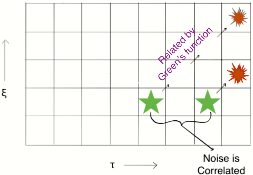
Figure 2 also illustrates the correlation introduced in the system due to colored noise. For a white noise profile, the two star noise sources will not be correlated and hence the charge fluctuation that has traveled will not have any correlation. But if we switch on colored noise, there will be a correlation between the two bursts.

In the Catteneo equation of motion for the charge current, the viscous current is given by Eq. (31). The evolution equation for charge fluctuations represented by $X=\tau\delta n_{Q}$ in momentum space is

	$\displaystyle\tau_{Q}\frac{\partial^{2}\tilde{X}}{\partial\tau^{2}}$	$\displaystyle+$	$\displaystyle\left(1+\frac{2\tau_{Q}}{\tau}\right)\frac{\partial\tilde{X}}{\partial\tau}+\frac{D_{Q}k_{\xi}^{2}}{\tau^{2}}\tilde{X}+(k_{x}^{2}+k_{y}^{2})D_{Q}\tilde{X}$		(34)
		$\displaystyle+$	$\displaystyle\frac{2D_{Q}\tau_{Q}(k_{x}^{2}+k_{y}^{2})}{\tau}(1+\tau_{Q}\partial_{\tau})^{-1}\tilde{X}$
		$\displaystyle=$	$\displaystyle-ik_{\xi}s\left[\tau_{Q}\frac{\partial\tilde{f}}{\partial\tau}+\left(1+\frac{\tau_{Q}}{\tau}\right)\tilde{f}\right]$
			$\displaystyle-is\bigg[(k_{x}\tilde{g}_{1}+k_{y}\tilde{g}_{2})(\tau+2\tau_{Q})$
			$\displaystyle+\tau_{Q}\tau\left(k_{x}\frac{\partial\tilde{g}_{1}}{\partial\tau}+k_{y}\frac{\partial\tilde{g}_{2}}{\partial\tau}\right)\bigg].$

To avoid a third-order differential equation we make the following approximation

$$(1+\tau_{Q}\partial_{\tau})^{-1}\simeq 1-\tau_{Q}\partial_{\tau}.$$

(35)

This is a good approximation when $\tau_{Q}<\tau$. The approximated charge conservation equation is

	$\displaystyle\tau_{Q}\frac{\partial^{2}\tilde{X}}{\partial\tau^{2}}$	$\displaystyle+$	$\displaystyle\left(1+2\frac{\tau_{Q}}{\tau}\right)\frac{\partial\tilde{X}}{\partial\tau}+\frac{D_{Q}k_{\xi}^{2}}{\tau^{2}}\tilde{X}+\frac{2D_{Q}\tau_{Q}(k_{x}^{2}+k_{y}^{2})}{\tau}\tilde{X}$		(36)
		$\displaystyle-$	$\displaystyle\frac{2D_{Q}\tau_{Q}^{2}(k_{x}^{2}+k_{y}^{2})}{\tau}\frac{\partial\tilde{X}}{\partial\tau}+D_{Q}(k_{x}^{2}+k_{y}^{2})\tilde{X}\qquad\qquad$
		$\displaystyle=$	$\displaystyle-ik_{\xi}s\left[\tau_{Q}\frac{\partial\tilde{f}}{\partial\tau}+\left(1+\frac{\tau_{Q}}{\tau}\right)\tilde{f}\right]$
			$\displaystyle-is\bigg[(k_{x}\tilde{g}_{1}+k_{y}\tilde{g}_{2})(\tau+2\tau_{Q})$
			$\displaystyle+\tau_{Q}\tau\left(k_{x}\frac{\partial\tilde{g}_{1}}{\partial\tau}+k_{y}\frac{\partial\tilde{g}_{2}}{\partial\tau}\right)\bigg].$

Eq. (36) is a complex SDE and is challenging to solve analytically. If we remove the dependence on the transverse coordinates it is possible to solve the SDE analytically, as was done in Ref. Kapusta and Plumberg 2018. With the inclusion of transverse coordinates, we will solve the SDE using direct numerical simulations on a discrete lattice. To ensure numerical convergence, we use $d\tau=0.003$ fm/$c$. Detailed numerical schemes are explained in Appendix B.

To generate a 2-point correlation in the form of Eq. (32) for the noise term $f(\tau,\xi)$ we need to solve an additional Langevin equation

$$f+\tau_{Q}\frac{\partial f}{\partial\tau}=\zeta$$

(37)

where $\zeta$ is a white noise such that

$$\langle\zeta(\tau)\rangle=0,\qquad\langle\zeta(\tau_{1})\zeta(\tau_{2})\rangle=M(\tau_{1})\delta(\tau_{1}-\tau_{2}).$$

(38)

Here $M(\tau)$ is the variance of the white noise $\zeta(\tau)$. The analytical solution of the Langevin equation is given by

$$\langle f(\tau_{1})f(\tau_{2})\rangle=\frac{M}{2\tau_{Q}}\left[e^{|\tau_{1}-\tau_{2}|/\tau_{Q}}-e^{(2\tau_{i}-\tau_{1}-\tau_{2})/\tau_{Q}}\right].$$

(39)

For illustration, Fig. 3 uses $M=1$ fm/$c$ and shows that the analytical solution and the numerical solution match each other. The noise that we need in this work is given by the 2-point correlation given in Eq. (33).

Note that this is the same correlation we need for both $g_{1}$ and $g_{2}$. Once we generate the noise terms we can simulate Eq. (36) for different values of $\tau_{Q}$ as shown in Fig. 4.

In the case of the Catteneo noise, the 2-point correlator shows noticeable differences from the results in the white noise limit. It is because the Catteneo noise introduces higher-order correlations that are not tracked by the hydro-kinetic equation, as shown in Fig. 5¹¹ 1 The actual values of the four-point function depends on the lattice spacing used in the simulation. With $\Delta x=0.013$ fm, we expect $\langle\zeta\zeta\zeta\zeta\rangle\propto 1/(\Delta x)^{2}\sim 6000$.. These higher-order correlations are generated from the Langevin equation in Eq. (37). The 4-point correlator of white noise shown in the figure should be strictly zero except when $\tau=\tau_{f}$. The numerical simulations reproduce that mathematical statement. The same 4-point correlator for Catteneo noise need not be zero because of higher-order correlations not present in white noise. This particular correlator is sufficient to exemplify that fact. Cumulants could also be used to illustrate that, but calculating them takes about two orders of magnitude more computational time to obtain the same accuracy. One can see that for Catteneo noise there is no fixed equilibrium value for any finite value of $k_{\xi}$. For a lower signal propagation speed, meaning larger $\tau_{Q}$, the magnitude of the 2-point correlation function $N$ is smaller at larger values of $k_{\xi}$. That arises from the nature of the self-correlation term as described in Ref. De et al. 2020.

The nature of the self-correlation is easiest to understand in the 1+1 D case. The mathematical expression for self-correlation is given by (Refs. Kapusta and Plumberg 2018; De et al. 2020).

$$\Big\langle\delta n_{Q}(\xi_{1},\tau_{f})\delta n_{Q}(\xi_{2},\tau_{f})\Big\rangle_{\text{self}}=\frac{\tau_{f}}{D_{Q}}\int\frac{dk}{2\pi}e^{ik(\xi_{1}-\xi_{2})}\\$$

$$\times\int\frac{d\tau^{\prime\prime}}{\tau^{\prime\prime}}\;\frac{\tilde{G}(-k,\tau_{f},\tau^{\prime\prime})}{ik}\;\langle f(\tau_{f})f(\tau^{\prime\prime})\rangle$$

(40)

The $\tilde{G}$ is a Green function, see Appendix A. Direct numerical simulations in Ref. De et al. 2020 showed how the self-correlation looks for various values of $\tau_{Q}$, as depicted in the Fig. 6.

One can see that as $\tau_{Q}\to 0$, the self-correlation looks more and more like a Dirac $\delta$- function. The absence of the Dirac $\delta$-function in the case of colored noise means that there is no fixed equilibrium value. The definition of self-correlation is straightforwardly extendable to the 3+1 D.

Self-correlation can be interpreted as the correlation of a charge fluctuation generated in $\xi_{1}$ at final time $\tau_{f}$ with another charge fluctuation generated in $\xi_{1}$ at a previous time but which has traveled to $\xi_{2}$ at $\tau_{f}$. It is nontrivial for colored noise because colored noise fluctuations in the same $\xi$ are correlated in time. Figure 7 gives an illustration of self-correlation.

Higher point correlations are also introduced because of causal diffusion. Specifically, the non-linear treatment of the white noise introduces the higher-order correlations.

Given the behavior of the 2-point correlator in the presence of colored noise, with a peak around $k_{*}$ and a decaying tail, it is interesting to disentangle the effects of causal diffusion and causal noise. Figure 8 shows the 2-point correlator as a function of $k_{\xi}$ for the following three cases:

1. 1.

   Causal diffusion and white noise.

2. 2.

   Usual diffusion and causal noise.

3. 3.

   Usual diffusion and white noise

First, consider case 1. Causal diffusion is an inefficient process compared to usual diffusion when it comes to distributing the charge buildup at a particular space point to neighboring points. In addition, white noise fluctuations at a particular point at a specific time are uncorrelated with whatever noise fluctuations that have originated at that point in previous times. This just means that there is continuous pumping of noise fluctuations at a space point through its temporal journey irrespective of the amount of charge buildup there. Causal diffusion does a limited redistribution of the charge buildup. Hence there is a peak in the 2-point correlation around the length scale $k_{*}$. This is further illustrated in Fig. 9 which is a plot of the 2-point correlator in coordinate space.

Now consider case 2. When we incorporate causal noise, the noise fluctuations that occur at a spatial point are correlated to the noise fluctuations that have already originated there in the previous moments. Hence a spatial point that has had a lot of charge buildup, because of recent large charge fluctuations, will not have large fluctuations at subsequent times because of the exponentially decaying correlation. In this case, the diffusion, either usual or causal, has enough time to distribute the charge buildup effectively. This is further illustrated in Fig. 10.

Both curves in Fig. 10 use the same causal noise and hence the self-correlation part for both the curves are the same. The presence of causal diffusion narrows the inverted Gaussian (which signifies the diffusion). Case 3 is the standard white noise result from Fig. 10 of Ref. De et al. 2020, specifically, the Dirac $\delta$-function minus a Gaussian. Here, the noise fluctuations pumped in by white noise is effectively dispersed away with infinite signal propagation speed by the usual diffusion process.

This brings us to our final point. The fluctuation-dissipation theorem tells us that causal noise and causal diffusion are inextricably present. Hence we expect both a peak in the two point correlator and a decaying tail at large $k_{\xi}$. Both may have phenomenological consequences.

Hydrodynamics is an effective theory that describes the behavior of quark-gluon plasma in a heavy-ion collision. With viscous hydrodynamics comes thermal noise that affect the macroscopic fluid variables. In this paper, we compared the two prevalent ways to study the evolution and effects of thermal fluctuations in relativistic hydrodynamics. The direct stochastic calculation is compared with the deterministic way of tracking the 2-point functions of hydrodynamic variables which are called hydro-kinetics in the literature. Here we considered the relatively simple case of a Bjorken evolution of a single conserved charge, including transverse fluctuations, and focus on the comparison of the 2-point charge correlation functions. We first perform comparisons using white noise and find exact agreements between the two approaches. This agreement is expected because white noise only introduces 2-point correlations. We then extend the stochastic hydrodynamics approach to study the evolution of colored (Catteneo) noise with the causal diffusion equation. The colored noise together with causal evolution results in significant deviations from the results at the white noise limit.

The main result of our work is that the colored noise evolved with the causal diffusion equation generates a peak structure around $k_{\xi}\sim k_{*}$ and decaying tail at large $k_{\xi}$ in the 2-point correlation function in the Fourier space as shown in Fig. 4. These features can be better understood in coordinate space. The peak around $k_{*}$ is a consequence of the correlation function being confined inside the light cone. The 2-point charge correlation function at large $k_{\xi}$ is no longer a constant in the causal case because the self-correlation has a finite extension in the Catteneo noise case. Even if the system was non-expanding, the Catteneo noise would have induced this feature. These features in the causal charge correlation functions could lead to phenomenological consequences in final-state particle correlations. Specifically, the enhancement and narrowing of the charge balance functions in the presence of colored noise has been discussed in Ref. De et al. 2020.

The quantity $k_{*}$ is an important emergent length scale in the dynamically evolving system. Modes with $k_{\xi}\gtrsim 0.5k_{*}$ remain in equilibrium whereas those with $k_{\xi}\lesssim 0.5k_{*}$ are pulled out of equilibrium because of the background expansion of the system. The value of $k_{*}$ should not change significantly in the Catteneo noise with causal diffusion. This is because the competition between the quenching rate for the fluctuations and the medium expansion rate is not affected a lot by the non-linearity introduced by the colored noise and causal equation of motion. The $k_{*}$ for the causal case will be a little less than that of the usual diffusion case. Hence, a possible future direction would be to study observables associated with $k_{*}$. Another interesting avenue would be to explore the emergent scales when a critical point is introduced into the equation of state. This question was investigated in Ref. Akamatsu et al. 2019.

It has been shown in this work that the hydro-kinetic approach is equivalent to solving the white noise SDE. It remains an open question whether the causal evolution and correlated color noise can be implemented in the hydro-kinetic approach. As shown in Fig. 5, the correlated Catteneo noise introduces higher-order correlations. We also find that the causal diffusion evolution introduces higher-order correlations because of its non-linear treatment of noise. It would be interesting to compare the higher-point correlation functions with the results from the hydro-kinetic approach in Ref. An et al. 2021.

Finally, it is clear from the discussion at the end of Sec. IV and Fig. 9 that considering causal diffusion without colored noise leads to a buildup of charge correlation in small $k_{\xi}$. The location of this buildup depends on grid size, which is unphysical. Causal diffusion and colored noise need to be considered as a package whenever we are considering the effects of stochastic noise on hydrodynamic variables. In the full-fledged causal Israel-Stewart hydrodynamics Young et al. 2015; Murase 2015; Singh et al. 2019; Sakai et al. 2020, stochastic fluctuations are sourced as white noises in the relaxation-type of equation of motion for shear stress tensor to generate the finite time correlations. Such treatment is consistent with the Catteneo noise generation in our case. One can go further and consider the Gurtin-Pipkin Gurtin and Pipkin 1968 noise which introduces a noise correlation in the spatial direction in addition to the correlation in time. Gurtin-Pipkin noise is in some sense more ‘physical’ and has been dealt with analytically in Ref. Kapusta and Young 2014a. Exploration with a noise profile with a spatial correlation is left to future work.

The authors thank Derek Teaney and Mayank Singh for their helpful discussions. This work was supported by the U.S. Department of Energy, Office of Science, Office of Nuclear Physics, under DOE Contract Nos. DE-FG02-87ER40328 and DE-SC0021969. C.S. acknowledges a DOE Office of Science Early Career Award. We acknowledge the Minnesota Supercomputing Institute (MSI) at the University of Minnesota for providing resources that contributed to the research results reported within this paper.

References

- Heinz and Snellings (2013) Ulrich Heinz and Raimond Snellings, “Collective flow and viscosity in relativistic heavy-ion collisions,” Ann. Rev. Nucl. Part. Sci. 63, 123–151 (2013), arXiv:1301.2826 [nucl-th] .
- Gale et al. (2013) Charles Gale, Sangyong Jeon, and Bjoern Schenke, “Hydrodynamic Modeling of Heavy-Ion Collisions,” Int. J. Mod. Phys. A 28, 1340011 (2013), arXiv:1301.5893 [nucl-th] .
- Shen and Yan (2020) Chun Shen and Li Yan, “Recent development of hydrodynamic modeling in heavy-ion collisions,” Nucl. Sci. Tech. 31, 122 (2020), arXiv:2010.12377 [nucl-th] .
- Pratt et al. (2015) Scott Pratt, Evan Sangaline, Paul Sorensen, and Hui Wang, “Constraining the Eq. of State of Super-Hadronic Matter from Heavy-Ion Collisions,” Phys. Rev. Lett. 114, 202301 (2015), arXiv:1501.04042 [nucl-th] .
- Bernhard et al. (2016) Jonah E. Bernhard, J. Scott Moreland, Steffen A. Bass, Jia Liu, and Ulrich Heinz, “Applying Bayesian parameter estimation to relativistic heavy-ion collisions: simultaneous characterization of the initial state and quark-gluon plasma medium,” Phys. Rev. C 94, 024907 (2016), arXiv:1605.03954 [nucl-th] .
- Bernhard et al. (2019) Jonah E. Bernhard, J. Scott Moreland, and Steffen A. Bass, “Bayesian estimation of the specific shear and bulk viscosity of quark–gluon plasma,” Nature Phys. 15, 1113–1117 (2019).
- Everett et al. (2021a) D. Everett et al. (JETSCAPE), “Phenomenological constraints on the transport properties of QCD matter with data-driven model averaging,” Phys. Rev. Lett. 126, 242301 (2021a), arXiv:2010.03928 [hep-ph] .
- Everett et al. (2021b) D. Everett et al. (JETSCAPE), “Multisystem Bayesian constraints on the transport coefficients of QCD matter,” Phys. Rev. C 103, 054904 (2021b), arXiv:2011.01430 [hep-ph] .
- Nijs et al. (2021a) Govert Nijs, Wilke van der Schee, Umut Gürsoy, and Raimond Snellings, “Bayesian analysis of heavy ion collisions with the heavy ion computational framework Trajectum,” Phys. Rev. C 103, 054909 (2021a), arXiv:2010.15134 [nucl-th] .
- Nijs et al. (2021b) Govert Nijs, Wilke van der Schee, Umut Gürsoy, and Raimond Snellings, “Transverse Momentum Differential Global Analysis of Heavy-Ion Collisions,” Phys. Rev. Lett. 126, 202301 (2021b), arXiv:2010.15130 [nucl-th] .
- Song et al. (2011) Huichao Song, Steffen A. Bass, Ulrich Heinz, Tetsufumi Hirano, and Chun Shen, “200 A GeV Au+Au collisions serve a nearly perfect quark-gluon liquid,” Phys. Rev. Lett. 106, 192301 (2011), [Erratum: Phys.Rev.Lett. 109, 139904 (2012)], arXiv:1011.2783 [nucl-th] .
- Shen et al. (2016) Chun Shen, Zhi Qiu, Huichao Song, Jonah Bernhard, Steffen Bass, and Ulrich Heinz, “The iEBE-VISHNU code package for relativistic heavy-ion collisions,” Comput. Phys. Commun. 199, 61–85 (2016), arXiv:1409.8164 [nucl-th] .
- Putschke et al. (2019) J. H. Putschke et al., “The JETSCAPE framework,” (2019), arXiv:1903.07706 [nucl-th] .
- Schenke et al. (2020) Bjoern Schenke, Chun Shen, and Prithwish Tribedy, “Running the gamut of high energy nuclear collisions,” Phys. Rev. C 102, 044905 (2020), arXiv:2005.14682 [nucl-th] .
- Young et al. (2015) C. Young, J. I. Kapusta, C. Gale, S. Jeon, and B. Schenke, “Thermally Fluctuating Second-Order Viscous Hydrodynamics and Heavy-Ion Collisions,” Phys. Rev. C 91, 044901 (2015), arXiv:1407.1077 [nucl-th] .
- Kapusta et al. (2012) J. I. Kapusta, B. Muller, and M. Stephanov, “Relativistic Theory of Hydrodynamic Fluctuations with Applications to Heavy Ion Collisions,” Phys. Rev. C 85, 054906 (2012), arXiv:1112.6405 [nucl-th] .
- Pratt and Young (2017) Scott Pratt and Clint Young, “Relating Measurable Correlations in Heavy Ion Collisions to Bulk Properties of Equilibrated QCD Matter,” Phys. Rev. C 95, 054901 (2017), arXiv:1612.08983 [nucl-th] .
- Pratt and Plumberg (2019) Scott Pratt and Christopher Plumberg, “Evolving Charge Correlations in a Hybrid Model with both Hydrodynamics and Hadronic Boltzmann Descriptions,” Phys. Rev. C 99, 044916 (2019), arXiv:1812.05649 [nucl-th] .
- Plumberg and Kapusta (2017) Christopher Plumberg and Joseph I. Kapusta, “Hydrodynamic fluctuations near a critical endpoint and Hanbury-Brown–Twiss interferometry,” Phys. Rev. C 95, 044910 (2017), arXiv:1702.01368 [nucl-th] .
- Bzdak et al. (2020) Adam Bzdak, Shinichi Esumi, Volker Koch, Jinfeng Liao, Mikhail Stephanov, and Nu Xu, “Mapping the Phases of Quantum Chromodynamics with Beam Energy Scan,” Phys. Rept. 853, 1–87 (2020), arXiv:1906.00936 [nucl-th] .
- Bluhm et al. (2020) Marcus Bluhm et al., “Dynamics of critical fluctuations: Theory – phenomenology – heavy-ion collisions,” Nucl. Phys. A 1003, 122016 (2020), arXiv:2001.08831 [nucl-th] .
- An et al. (2022) Xin An et al., “The BEST framework for the search for the QCD critical point and the chiral magnetic effect,” Nucl. Phys. A 1017, 122343 (2022), arXiv:2108.13867 [nucl-th] .
- Kapusta and Plumberg (2018) Joseph I. Kapusta and Christopher Plumberg, “Causal Electric Charge Diffusion and Balance Functions in Relativistic Heavy Ion Collisions,” Phys. Rev. C 97, 014906 (2018), [Erratum: Phys.Rev.C 102, 019901 (2020)], arXiv:1710.03329 [nucl-th] .
- Pratt et al. (2018) Scott Pratt, Jane Kim, and Christopher Plumberg, “Evolution of Charge Fluctuations and Correlations in the Hydrodynamic Stage of Heavy Ion Collisions,” Phys. Rev. C 98, 014904 (2018), arXiv:1712.09298 [nucl-th] .
- Pratt and Plumberg (2020) Scott Pratt and Christopher Plumberg, “Determining the Diffusivity for Light Quarks from Experiment,” Phys. Rev. C 102, 044909 (2020), arXiv:1904.11459 [nucl-th] .
- De et al. (2020) Aritra De, Christopher Plumberg, and Joseph I. Kapusta, “Calculating Fluctuations and Self-Correlations Numerically for Causal Charge Diffusion in Relativistic Heavy-Ion Collisions,” Phys. Rev. C 102, 024905 (2020), arXiv:2003.04878 [nucl-th] .
- Nahrgang and Bluhm (2020) Marlene Nahrgang and Marcus Bluhm, “Modeling the diffusive dynamics of critical fluctuations near the QCD critical point,” Phys. Rev. D 102, 094017 (2020), arXiv:2007.10371 [nucl-th] .
- Rajagopal et al. (2020) Krishna Rajagopal, Gregory Ridgway, Ryan Weller, and Yi Yin, “Understanding the out-of-equilibrium dynamics near a critical point in the QCD phase diagram,” Phys. Rev. D 102, 094025 (2020), arXiv:1908.08539 [hep-ph] .
- Du et al. (2020) Lipei Du, Ulrich Heinz, Krishna Rajagopal, and Yi Yin, “Fluctuation dynamics near the QCD critical point,” Phys. Rev. C 102, 054911 (2020), arXiv:2004.02719 [nucl-th] .
- Du et al. (2021) Lipei Du, Xin An, and Ulrich Heinz, “Baryon transport and the QCD critical point,” Phys. Rev. C 104, 064904 (2021), arXiv:2107.02302 [hep-ph] .
- Murase (2015) Koichi Murase, Causal hydrodynamic fluctuations and their effects on high-energy nuclear collisions, Ph.D. thesis, Tokyo U. (2015).
- Singh et al. (2019) Mayank Singh, Chun Shen, Scott McDonald, Sangyong Jeon, and Charles Gale, “Hydrodynamic Fluctuations in Relativistic Heavy-Ion Collisions,” Nucl. Phys. A 982, 319–322 (2019), arXiv:1807.05451 [nucl-th] .
- Sakai et al. (2020) Azumi Sakai, Koichi Murase, and Tetsufumi Hirano, “Rapidity decorrelation of anisotropic flow caused by hydrodynamic fluctuations,” Phys. Rev. C 102, 064903 (2020), arXiv:2003.13496 [nucl-th] .
- Sakai et al. (2021) Azumi Sakai, Koichi Murase, and Tetsufumi Hirano, “Effects of hydrodynamic and initial longitudinal fluctuations on rapidity decorrelation of collective flow,” (2021), arXiv:2111.08963 [nucl-th] .
- Akamatsu et al. (2017) Yukinao Akamatsu, Aleksas Mazeliauskas, and Derek Teaney, “A kinetic regime of hydrodynamic fluctuations and long time tails for a Bjorken expansion,” Phys. Rev. C 95, 014909 (2017), arXiv:1606.07742 [nucl-th] .
- Stephanov and Yin (2018) M. Stephanov and Y. Yin, “Hydrodynamics with parametric slowing down and fluctuations near the critical point,” Phys. Rev. D 98, 036006 (2018), arXiv:1712.10305 [nucl-th] .
- Akamatsu et al. (2019) Yukinao Akamatsu, Derek Teaney, Fanglida Yan, and Yi Yin, “Transits of the QCD critical point,” Phys. Rev. C 100, 044901 (2019), arXiv:1811.05081 [nucl-th] .
- An et al. (2019) Xin An, Gokce Basar, Mikhail Stephanov, and Ho-Ung Yee, “Relativistic Hydrodynamic Fluctuations,” Phys. Rev. C 100, 024910 (2019), arXiv:1902.09517 [hep-th] .
- Martinez et al. (2019) M. Martinez, T. Schäfer, and V. Skokov, “Critical behavior of the bulk viscosity in QCD,” Phys. Rev. D 100, 074017 (2019), arXiv:1906.11306 [hep-ph] .
- An et al. (2020) Xin An, Gökçe Başar, Mikhail Stephanov, and Ho-Ung Yee, “Fluctuation dynamics in a relativistic fluid with a critical point,” Phys. Rev. C 102, 034901 (2020), arXiv:1912.13456 [hep-th] .
- Martinez and Schäfer (2017) Mauricio Martinez and Thomas Schäfer, “Hydrodynamic tails and a fluctuation bound on the bulk viscosity,” Phys. Rev. A 96, 063607 (2017), arXiv:1708.01548 [cond-mat.quant-gas] .
- Bjorken (1983) J. D. Bjorken, “Highly Relativistic Nucleus-Nucleus Collisions: The Central Rapidity Region,” Phys. Rev. D 27, 140–151 (1983).
- Kapusta and Young (2014a) J. I. Kapusta and C. Young, “Causal Baryon Diffusion and Colored Noise,” Phys. Rev. C 90, 044902 (2014a), arXiv:1404.4894 [nucl-th] .
- Kapusta and Young (2014b) J. I. Kapusta and C. Young, “Causal Baryon Diffusion and Colored Noise for Heavy Ion Collisions,” Nucl. Phys. A 931, 1051–1055 (2014b), arXiv:1409.1957 [nucl-th] .
- Cattaneo et al. (1958) C. Cattaneo, J.K. de Fériet, and Académie des sciences (France), Sur une forme de l’équation de la chaleur éliminant le paradoxe d’une propagation instantanée, Comptes rendus hebdomadaires des séances de l’Académie des sciences (Gauthier-Villars, 1958).
- An et al. (2021) Xin An, Gökçe Başar, Mikhail Stephanov, and Ho-Ung Yee, “Evolution of Non-Gaussian Hydrodynamic Fluctuations,” Phys. Rev. Lett. 127, 072301 (2021), arXiv:2009.10742 [hep-th] .
- Gurtin and Pipkin (1968) M.E. Gurtin and A.C. Pipkin, “A general theory of heat conduction with finite wave speeds.” Arch. Rational Mech. Anal. 31, 113–126 (1968).