Nudged elastic band approach to nuclear fission pathways

Eric Flynn Affiliation: Department of Physics and Astronomy and FRIB/NSCL Laboratory, Michigan State University, East Lansing, Michigan 48824, USA Daniel Lay Affiliation: Department of Physics and Astronomy and FRIB/NSCL Laboratory, Michigan State University, East Lansing, Michigan 48824, USA Sylvester Agbemava Affiliation: FRIB/NSCL Laboratory, Michigan State University, East Lansing, Michigan 48824, USA Pablo Giuliani Affiliation: FRIB/NSCL Laboratory, Michigan State University, East Lansing, Michigan 48824, USA Affiliation: Department of Statistics and Probability, Michigan State University, East Lansing, Michigan 48824, USA Kyle Godbey Affiliation: FRIB/NSCL Laboratory, Michigan State University, East Lansing, Michigan 48824, USA Witold Nazarewicz Affiliation: Department of Physics and Astronomy and FRIB/NSCL Laboratory, Michigan State University, East Lansing, Michigan 48824, USA Jhilam Sadhukhan Affiliation: Physics Group, Variable Energy Cyclotron Centre, Kolkata 700064, India Affiliation: Homi Bhabha National Institute, Mumbai 400094, India

August 11, 2026

Abstract

Background: The nuclear fission process is a dramatic example of the large-amplitude collective motion in which the nucleus undergoes a series of shape changes before splitting into distinct fragments. This motion can be represented by a pathway in the many-dimensional space of collective coordinates. The collective action along the fission pathway determines the spontaneous fission half-lives as well as mass and charge distributions of fission fragments.
Purpose: We study the performance and precision of various methods to determine the minimum-action and minimum-energy fission trajectories in the collective space.
Methods: We apply the nudged elastic band method (NEB), grid-based methods, and Euler-Lagrange approach to the collective action minimization in two- and three-dimensional collective spaces.
Results: The performance of various approaches to the fission pathway problem is assessed by studying the collective motion along both analytic energy surfaces and realistic potential energy surfaces obtained with the Skyrme-Hartree-Fock-Bogoliubov theory. The uniqueness and stability of the solutions is studied. The NEB method is capable of efficient determination of the exit points on the outer turning surface that characterize the most probable fission pathway and constitute the key input for fission studies. This method can also be used to accurately compute the critical points (i.e., local minima and saddle points) on the potential energy surface of the fissioning nucleus that determine the static fission path. The dynamic programming method also performs quite well and it can be used in many-dimensional cases to provide initial conditions for the NEB calculations.
Conclusions: The NEB method is the tool of choice for finding the least-action and minimum-energy fission trajectories. It will be particularly useful in large-scale fission calculation of superheavy nuclei and neutron-rich fissioning nuclei contributing to the astrophysical r-process recycling.

I Introduction

Fission is a fundamental nuclear decay that is important in many areas of science, ranging from structure and stability of heavy and superheavy nuclei Krappe and Pomorski 2012; Schmidt and Jurado 2018; Giuliani et al. 2019 to studies devoted to physics beyond the standard model of particle physics Vogel et al. 2015 and the synthesis of heavy elements Horowitz et al. 2019; Vassh et al. 2019; Giuliani et al. 2020.

Theoretically, the nuclear fission process is an example of the nuclear large-amplitude collective motion originating from the single-particle motion of individual nucleons. Due to the complexity of this process, our understanding of nuclear fission is still incomplete. For the state of affairs in this field, we refer to the recent review Schunck and Robledo 2016; Bender et al. 2020.

When it comes to realistic predictions, the self-consistent nuclear energy density functional (EDF) method Bender et al. 2003; Schunck 2019 has proven to be very successful in terms of quantitative reproduction of fission lifetimes and fragment yields. Unfortunately, realistic self-consistent fission calculations in a multidimensional collective space, based on the microscopic input, are computationally expensive when it comes to large-scale theoretical fission surveys. Given the computational cost of microscopic methods and the large number of fissioning nuclei that are, e.g., expected to contribute to the astrophysical r-process nucleosynthesis, calculations have mostly relied on simple parametrizations or highly phenomenological models. The new perspective is offered by state-of-the-art theoretical frameworks and modern computational techniques that promise to speed up the calculations to be able to carry out quantified global fission surveys for multiple inputs Bender et al. 2020.

This study is concerned with finding the optimal pathway during the tunneling motion phase of spontaneous fission (SF). Such a trajectory, dubbed the least-action path (LAP), is obtained by minimizing the collective action in a many-dimensional collective space Kapur and Peierls 1937; Brack et al. 1972. A number of techniques have been proposed to deal with this challenging task. In the early application Ledergerber and Pauli 1973, the trial pathways were assumed in a parametrized form and the LAP was obtained by minimizing the penetration integral with respect to the variational parameters. Grid-based techniques such as the dynamic-programming Baran et al. 1981 and Ritz Baran 1978 methods have been used in numerous EDF calculations of LAPs Sadhukhan et al. 2013; Sadhukhan et al. 2014; Sadhukhan et al. 2016; Sadhukhan et al. 2017; Zhao et al. 2015; Zhao et al. 2016; Mercier et al. 2021. In Refs. Schmid 1986; Eckern and Schmid 1992; Kindo and Iwamoto 1989; Iwamoto and Tomita 1992; Iwamoto 1994; Scamps and Hagino 2015 LAPs were obtained by solving the eikonal equation by the method of characteristics. Effectively, this method can be related to a quantum mechanical propagation in imaginary time that amounts to solving the classical equations of motion in an inverted potential. Within this approach, only one trajectory, called the escape path, arrives at the outer turning surface with zero velocity. Other trajectories, corresponding to different initial conditions, cannot reach the outer turning surface.

In this paper, we compare grid-based approaches to the LAPs with the nudged elastic band (NEB) method that was originally formulated in the context of molecular systems Garrett and Truhlar 1983; Mills and Jónsson 1994; Mills et al. 1995; Jónsson et al.. In NEB, the minimum action path can be obtained iteratively by continuously shifting the pathway to the nearest minimum action path Henkelman et al. 2000; Henkelman and Jónsson 2000; ASE. A similar approach is a growing string method Peters et al. 2004. To provide more insights, we also employ the Euler-Lagrange (EL) method to compute the stationary action path.

In addition to the LAP, another characteristic trajectory in the collective space is the minimum-energy path (MEP), sometimes referred to as the static path. The MEP can serve as a first, rough approximation to the LAP. It is obtained by computing the steepest descent line on the potential energy surface, which passes through the local minima and saddle points. To find the MEP, a flooding, or watershed, algorithm has been applied Mamdouh et al. 1998; Möller et al. 2001; Iwamoto et al. 2002; Möller et al. 2004; Wang et al. 2019. The NEB approach can also be adopted to find the MEP and saddle points Ásgeirsson et al. 2021. (For a review of modern optimization methods for finding MEPs, see Sheppard et al. 2008; Moré and Munson 2004.)

This paper is organized as follows. In Sec. II we define the basics concepts of the nuclear EDF approach as applied to nuclear fission. Section III describes the path-optimization methods used. The results of our calculations and an analysis of trends are presented in Sec. IV. Finally, Sec. V contains the conclusions of this work.

II Nuclear EDF approach to spontaneous fission

The main ingredients for a theoretical determination of SF lifetimes are the collective potential energy surface (PES) and the inertia tensor. To compute the PES, one solves the constrained Hartree-Fock-Bogoliubov (HFB) equations with the realistic energy density functional in the space of collective coordinates $\mbox{\boldmath$q$}\equiv\{q_{i}\}$ . These are usually represented by the expectation values of the quadrupole moment operator $\hat{Q}_{20}$ (elongation), quadrupole moment operator $\hat{Q}_{22}$ (triaxiality), octupole moment operator $\hat{Q}_{30}$ (mass-asymmetry), and the particle-number dispersion term $\lambda_{2\tau}(\hat{N}^{2}_{\tau}-\langle\hat{N}_{\tau}\rangle^{2})$ ( $\tau=n,p)$ that controls dynamic pairing correlations Vaquero et al. 2011; Vaquero et al. 2013; Sadhukhan et al. 2014. In some cases one also considers the hexadecapole moment $Q_{40}$ (necking coordinate) Warda et al. 2012. That is, in practical applications, we consider 2-5 collective coordinates which describe the collective motion of the system. Figure 1 shows a representative PES of ²⁵⁶Fm in the space of $Q_{20}\equiv\langle\hat{Q}_{20}\rangle$ and $Q_{30}\equiv\langle\hat{Q}_{30}\rangle$ .

Refer to caption — Figure 1: Potential energy surface of ²⁵⁶Fm calculated with nuclear EDF method using the D1S parametrization of the Gogny interaction Berger et al. 1984 in the space of two collective coordinates: $Q_{20}$ (elongation) and $Q_{30}$ (mass asymmetry). The static fission pathways are marked by solid lines: red (symmetric pathway) and green (asymmetric pathway). The outer turning line (OTL) is indicated, together with the outer turning points associated with the static pathways. For simplicity, we assume that the inner turning point corresponds to the ground-state configuration (i.e., $E_{0}=0$ ). The high-energy region that is practically not accessible during collective motion is indicated in black. The intersections of fission pathways with outer turning points are indicated by dots; these are important for determining fission fragment yields Sadhukhan et al. 2020; Sadhukhan et al. 2022.

The collective inertia (or mass) tensor $\mathcal{M}_{ij}(\mbox{\boldmath$q$})$ is obtained from the self-consistent densities by employing the the adiabatic time-dependent HFB approximation (ATDHFB) Baran et al. 2011; Giuliani and Robledo 2018; Washiyama et al. 2021. In this study, we use the non-perturbative cranking approximation Baran et al. 2011:

\mathcal{M}_{ij}(\mbox{\boldmath$q$})=\frac{\hbar^{2}}{2\dot{q}_{i}\dot{q}_{j}}\sum_{\alpha\beta}\frac{\left(F^{i*}_{\alpha\beta}F^{j}_{\alpha\beta}+F^{i}_{\alpha\beta}F^{j*}_{\alpha\beta}\right)}{E_{\alpha}+E_{\beta}},

(1)

where $q_{i}$ is the collective coordinate, $\dot{q}_{i}$ represents the time derivative of $q_{i}$ , and $E_{\alpha}$ are one-quasiparticle energies of HFB eigenstates $|\alpha\rangle$ . The matrices $F^{i}$ are given by

\frac{F^{i*}}{\dot{q}_{i}}=A^{T}\frac{\partial\kappa^{*}}{\partial q_{i}}A+A^{T}\frac{\partial\rho^{*}}{\partial q_{i}}B-B^{T}\frac{\partial\rho}{\partial q_{i}}A-B^{T}\frac{\partial\kappa}{\partial q_{i}}B,

(2)

where $A$ and $B$ are the matrices of the Bogoliubov transformation, and $\rho$ and $\kappa$ are particle and pairing density matrices, respectively, determined in terms of $A$ and $B$ . Derivatives of the density matrices with respect to collective coordinates are calculated by employing the three-point Lagrange formula. It is important to remark that rapid variations in $\mathcal{M}_{ij}$ are expected in the regions of configuration changes (level crossings) due to strong variations of density derivatives in (2) associated with structural rearrangements Ledergerber and Pauli 1973; Sadhukhan et al. 2013.

Since SF is a quantum-mechanical tunneling process and the fission barriers are usually both high and wide, the SF lifetime is obtained semi-classically Brack et al. 1972 as $T_{1/2}=\ln 2/(nP)$ , where $n$ is the number of assaults on the fission barrier per unit time and $P$ is the penetration probability given by

P=\left(1+\exp{[2S(L_{\rm min})]}\right)^{-1},

(3)

where $L_{\rm min}$ is the path that minimizes the fission action integral calculated along the one-dimensional trajectory $L(s)$ in the multidimensional collective space:

S(L)=\frac{1}{\hbar}\int_{s_{\rm in}}^{s_{\rm out}}{\cal S}(s)\,ds,

(4)

where

{\cal S}(s)=\sqrt{2\mathcal{M}_{\text{eff}}(s)\left(V_{\text{eff}}(s)-E_{0}\right)}

(5)

with $V_{\text{eff}}(s)$ and $\mathcal{M}_{\text{eff}}(s)$ being the effective potential energy and inertia along the fission path $L(s)$ , respectively. $V_{\text{eff}}$ can be obtained by subtracting the vibrational zero-point energy from the total HFB energy. (In the examples considered in this paper we assume the zero-point energy to be zero.) The integration limits $s_{\rm in}$ and $s_{\rm out}$ correspond to the classical inner and outer turning points, respectively, defined by $V_{\text{eff}}(s)=E_{0}$ on the two extremes of the fission path, see Fig. 1. The collective ground state (g.s.) energy is $E_{0}$ , and $ds$ is the element of length along $L(s)$ . A one-dimensional path $L(s)$ can be defined in the multidimensional collective space by specifying the collective variables $\mbox{\boldmath$q$}(s)$ as functions of path’s length $s$ . The expression for $\mathcal{M}_{\text{eff}}$ is Baran et al. 2005:

\mathcal{M}_{\text{eff}}(s)=\sum_{ij}\mathcal{M}_{ij}(\mbox{\boldmath$q$})\frac{dq_{i}}{ds}\frac{dq_{j}}{ds}.

(6)

The least-action path (LAP) $L_{\rm min}$ is obtained by minimizing the action integral (4) with respect to all possible trajectories $L$ that connect the lines/surfaces of inner turning points $s_{\rm in}$ and outer turning points $s_{\rm out}$ Sadhukhan et al. 2013. However, as discussed in Refs. Schmid 1986; Eckern and Schmid 1992 and this paper, only the pathways related to the exit points are stationary. The MEP can instead be described as the union of steepest descent paths from the saddle point(s) to the minima. The corresponding trajectory $\mbox{\boldmath$q$}(s)$ satisfies

\displaystyle\frac{d\mbox{\boldmath$q$}}{ds}\propto\mbox{\boldmath$\nabla$}V\big(\mbox{\boldmath$q$}(s)\big)

(7)

which characterizes a path of steepest descent on a surface $V(\mbox{\boldmath$q$})$ Quapp and Heidrich 1984. For the NEB, one finds the MEP by allowing the elements of the path to follow the gradient of the PES in their immediate vicinity. We shall assume that the PES in the tunneling region is free from discontinuities associated with rapid configuration changes Dubray and Regnier 2012; Zdeb et al. 2021; Lau et al. 2021. This assumption is usually valid because of non-vanishing pairing correlations inside the potential barrier. It is also to be noted that, as in any optimization/minimization approach, the stationary path determined numerically corresponds to a local action minimum, which is not guaranteed to be the global minimum. Moreover, there could be many stationary pathways representing different fission modes, see Fig. 2. To simplify notation, we assume in the following discussions that the stationary action path found by our algorithms is indeed the LAP.

Since ${\cal S}(s)=0$ on the outer turning surface $V(\mbox{\boldmath$q$})=E_{0}$ , it follows that paths moving on the surface $V(\mbox{\boldmath$q$})=0$ do not contribute to the action. This is illustrated in Fig. 2 by the path connecting the g.s. and, for example, the purple star labeled (3). Such a path consists of the cyan curve – the exit trajectory – and the green dashed line, connecting (1) with (3) through the OTL, which results in the same action integral as the exit trajectory.

III Methods/algorithms

All path-optimization methods described in the following subsections, bar the EL method, have a reference implementation included in the python package, PyNEB PyN.

III.1 Nudged Elastic Band

The NEB method was originally formulated to provide a smooth transition of a molecular system on a potential energy surface from the reactant to the product state Mills and Jónsson 1994; Mills et al. 1995; Jónsson et al.. Upon application of this variant of the NEB method, one obtains the MEP as well as a series of “images” of the molecular system as it transitions along the path. The NEB technique has been subsequently refined, with improved numerical stability Henkelman and Jónsson 2000 and a more accurate determination of a saddle point Henkelman et al. 2000 being two key advances towards a more widely applicable numerical approach for MEP determination.

To obtain the LAP, the procedure must be modified such that the images move towards the minimum of the action Ásgeirsson et al. 2018 which amounts to replacing the standard gradient of the PES with the gradient of the action

\mbox{\boldmath$g$}_{i}=-\mbox{\boldmath$\nabla$}_{i}S

(8)

with respect to the image $\mbox{\boldmath$q$}_{i}$ . With this prescription, the images will settle to the LAP in the collective space.

While the NEB method will, by design, drive the line of images towards either the MEP or LAP, the iterative scheme chosen greatly impacts the total number of iterations required before the solution converges. In the early implementations, a simple velocity Verlet algorithm Verlet 1967 was used to adjust the position of the images step to step Mills and Jónsson 1994; Mills et al. 1995; Jónsson et al.; Henkelman and Jónsson 2000; Henkelman et al. 2000. This approach is robust and relatively stable, though the convergence can be slow for flatter surfaces where the images are not pulled strongly to their optimal positions. To aid this process, the Fast Inertial Relaxation Engine (FIRE) was proposed Bitzek et al. 2006 to accelerate convergence without sacrificing stability. The method was subsequently updated Guénolé et al. 2020 to further improve performance. Indeed, in our tests, the inertial algorithm regularly outperforms the velocity Verlet algorithm by an-order-of-magnitude reduction in iterations at the same convergence criteria.

With this, our implementation of the NEB approach is defined. The algorithm itself is outlined in Algorithm 1 in SM SM. The force used in the optimization step for each image, $\mbox{\boldmath$F$}_{i}^{\rm opt}$ , is constructed by adding the perpendicular component of the action gradient to the spring force $\mbox{\boldmath$F$}_{i}^{k}$ between the images,

\mbox{\boldmath$F$}_{i}^{k}=k(|\mbox{\boldmath$q$}_{i+1}-\mbox{\boldmath$q$}_{i}|-|\mbox{\boldmath$q$}_{i}-\mbox{\boldmath$q$}_{i-1}|)\mbox{\boldmath$\tau_{i}$},

(9)

where $k$ is a tunable parameter that controls the strength of the spring force and $\tau_{i}$ is the unit vector tangent to the line of images from image $i-1$ to image $i+1$ . The spring force on the endpoints is defined differently:

\mbox{\boldmath$F$}_{1}^{k}=k|\mbox{\boldmath$q$}_{2}-\mbox{\boldmath$q$}_{1}|,\quad\mbox{\boldmath$F$}_{N}^{k}=k|\mbox{\boldmath$q$}_{N}-\mbox{\boldmath$q$}_{N-1}|.

(10)

The total force acting on the interior images is then

\displaystyle\mbox{\boldmath$F$}_{i}^{\rm opt}=\mbox{\boldmath$F$}^{k}_{i}+\mbox{\boldmath$g$}_{i}^{\perp}.

(11)

The NEB approach is illustrated in Fig. 2 for the case of bimodal tunneling from the g.s. minimum to the OTL on an analytic PES defined by:

	$\displaystyle V(\mbox{\boldmath$q$})$	$\displaystyle=3.17+2e^{-5\big((x-1)^{2}+(y-\frac{1}{2})^{2}\big)}-3e^{-(x^{2}+y^{2})}$
		$\displaystyle-\frac{1}{2}(3x+y),$		(12)

where $\mbox{\boldmath$q$}=(x,y)$ . The inset shows the forces on the images of the NEB grey path, which has not converged yet to the black path. The spring force $\boldsymbol{F}^{k}_{i}$ keeps the images from drifting too much from each other, while the perpendicular part of the action gradient $\boldsymbol{g}_{i}^{\perp}$ pushes them towards the nearest stationary action path. This example shows that the NEB algorithm, depending on the initial locations of the images, will converge to a local stationary path, not necessarily the least action path.

For the endpoint, $i=N$ , one can choose to either fix the position of the image or to allow the image to move towards the outer turning surface. In the second case, a harmonic restraint term is added to the spring force to construct $\mbox{\boldmath$F$}_{N}^{\rm opt}$ ,

\vec{F}_{N}^{\rm opt}=\vec{F}_{N}^{k}-\left[\vec{F}_{N}^{k}\cdot\mbox{\boldmath$f$}(\mbox{\boldmath$q$}_{N})-\eta(V(\mbox{\boldmath$q$})-E)\right]\mbox{\boldmath$f$}(\mbox{\boldmath$q$}_{N}),

(13)

where $\mbox{\boldmath$f$}=-\mbox{\boldmath$\nabla$}V/|\mbox{\boldmath$\nabla$}V|$ and $\eta$ determines the strength of the harmonic restraint term Ásgeirsson et al. 2018. This force pulls the endpoint $i=N$ very quickly to the outer turning surface and helps find the optimal outer turning point.

The default iteration scheme used in our implementation is the inertial algorithm mentioned above, though a standard Verlet minimizer is also included in the PyNEB python package PyN. The structure of the NEB solver is modular and allows for the simple replacement of components like the minimizer, allowing for easy checks on the convergence and parameters that describe the iterative scheme.

III.2 Grid-Based Methods

Some traditional methods to compute the LAP begin by computing the PES and the collective inertia on a grid of collective coordinates. The calculation of the LAP is then reduced to finding the path through the grid points that minimizes a discrete approximation of the action. Two methods that we have benchmarked are the dynamic programming method (DPM) Baran et al. 1981, and Dijkstra’s algorithm (DA) Dijkstra 1959. Here, both will be described for two-dimensional (2D) grid, with points labelled by $\mbox{\boldmath$q$}_{ij}=(x_{i},y_{j})$ ( $i=1,\ldots,N$ , $j=1,\ldots,M$ ). Both methods can be straightforwardly extended to a higher-dimensional grid.

Dynamic programming is a general mathematical technique for solving multi-decision problems by breaking the problem down into simpler overlapping sub-problems. It was first adapted to the action integral minimization in Ref. Baran et al. 1981 and used in Sadhukhan et al. 2013 to determine the LAP. This adaptation is what we refer to as the DPM.

The DPM approximates the LAP between an initial point, $\mbox{\boldmath$q$}_{\textrm{in}}$ , and a final point, $\mbox{\boldmath$q$}_{\textrm{fin}}$ . This method finds paths that traverse diagonally from a given cell: from cell $\mbox{\boldmath$q$}_{ij}$ , only cells $\mbox{\boldmath$q$}_{i+1,j}$ can be reached, for $j=1,\ldots,M$ . The allowed cells are highlighted in red in Fig. 3. The LAP from $\mbox{\boldmath$q$}_{\textrm{in}}$ to $\mbox{\boldmath$q$}_{\textrm{fin}}$ is constructed iteratively as follows: for a cell $\mbox{\boldmath$q$}_{ij}$ , there are $M$ possible paths, each passing through a cell at $x_{i-1}$ . The LAP from $\mbox{\boldmath$q$}_{\textrm{in}}$ to $\mbox{\boldmath$q$}_{ij}$ is selected and stored in memory. This is repeated for every cell with $x=x_{i}$ , for a total of $M$ possible paths. Once $\mbox{\boldmath$q$}_{\textrm{fin}}$ is reached, there are only $MN$ paths (out of a total of $M^{N}$ paths), and the LAP is selected from these. The DPM algorithm is detailed in Algorithm 2 in SM SM.

Dijkstra’s method Dijkstra 1959 is similar to DPM, in that it breaks down the large optimization problem into a set of smaller problems. Given a cell $\mbox{\boldmath$q$}_{ij}$ , the action to every neighbor $\mbox{\boldmath$q$}_{i^{\prime}j^{\prime}}$ is calculated as if the path to $\mbox{\boldmath$q$}_{i^{\prime}j^{\prime}}$ passes through $\mbox{\boldmath$q$}_{ij}$ . If this action integral is smaller than that along the current path to $\mbox{\boldmath$q$}_{i^{\prime}j^{\prime}}$ , $\mbox{\boldmath$q$}_{i^{\prime}j^{\prime}}$ is said to come from $\mbox{\boldmath$q$}_{ij}$ . This is repeated, starting from $\mbox{\boldmath$q$}_{\textrm{in}}$ , until $\mbox{\boldmath$q$}_{\textrm{fin}}$ is reached. Figure 3 shows the nearest-neighbors of $\mbox{\boldmath$q$}_{ij}$ (the cell marked in green) in a blue square. Dijkstra’s algorithm is described in Algorithm 3 in the SM SM.

Dijkstra’s algorithm can find paths that pass through multiple cells with the same $x_{i}$ value, or even paths that backtrack. DPM cannot find such paths. However, DPM can find paths that jump from $\mbox{\boldmath$q$}_{ij}$ to $\mbox{\boldmath$q$}_{i+1,j^{\prime}}$ , for any $j^{\prime}$ , while Dijkstra’s algorithm is limited to $j^{\prime}=j-1,j,j+1$ (see Fig. 3). For fission calculations, one frequently takes the $x$ coordinate as the quadrupole moment $Q_{20}$ , and fission can be viewed as collective motion in which $Q_{20}$ continuously increases towards scission. So, the paths that Dijkstra’s algorithm can find, that DPM cannot, are rather unlikely. In general DPM tends to find paths with a smaller action than Dijkstra’s algorithm, see Sec. IV.

III.3 Euler Lagrange Equations

In order to find the LAP for the functional (4) using the EL equations Weinstock 1974, we first parametrize the trajectory $q$ by a time variable $t$ , i.e., $\mbox{\boldmath$q$}=\mbox{\boldmath$q$}(t)$ with $t\in[0,t_{f}]$ . This is done in order to explicitly account for the arclength $ds=(\sum dq_{i}^{2})^{1/2}$ . In terms of $t$ , the action integral (4) reads:

\begin{split}&S(L)=\\ &\int_{0}^{t_{f}}\sqrt{2\big(V_{\text{eff}}[\mbox{\boldmath$q$}(t)]-E_{0}\big)}\Big(\sum_{ij}^{n}\mathcal{M}_{ij}[\mbox{\boldmath$q$}(t)]\dot{q}_{i}\dot{q}_{j}\Big)^{1/2}dt\\ &=\int_{0}^{t_{f}}\mathcal{L}(\mbox{\boldmath$q$},\dot{\mbox{\boldmath$q$}})dt,\end{split}

(14)

where $\dot{q}_{i}\equiv dq_{i}/dt$ , and $\mathcal{L}$ is the corresponding Lagrangian. The associated EL equation can be written as:

\frac{\partial\mathcal{L}}{\partial q_{i}}=\frac{d}{dt}\Big(\frac{\partial\mathcal{L}}{\partial\dot{q}_{i}}\Big),

(15)

with the boundary conditions: $\mbox{\boldmath$q$}(t=0)=\mbox{\boldmath$q$}_{\text{in}}$ (the initial location) and $\mbox{\boldmath$q$}(t=t_{f})=\mbox{\boldmath$q$}_{\text{{fin}}}$ (the final location).

In order to numerically solve Eq. (15) we use the shooting method Sho. That is, we start at the initial position $\mbox{\boldmath$q$}_{\text{in}}$ and vary the direction and orientation of the initial “velocity” $\dot{\mbox{\boldmath$q$}}(t=0)$ . We use a numerical differential equation solver to propagate the solution until we find an initial condition that satisfies $\mbox{\boldmath$q$}(t_{f})=\mbox{\boldmath$q$}_{\textrm{fin}}$ . Finding such initial conditions can present some challenges, which we discuss in the SM SM.

The EL approach is equivalent to what is done in Ref. Schmid 1986 where the eikonal equation is solved by the method of characteristics. Each different trajectory obtained by varying $\dot{\mbox{\boldmath$q$}}(t=0)$ corresponds to one of the characteristics of the leading order (cf. Eqs.(2.8) and (4.3) of Schmid 1986). It is worth noting that if the imaginary part of the phase of the wave function $W(\boldsymbol{q})$ is negligible, as is the case of the motion in the deep subbarrier region, then the eikonal equation for $W$ is a valid approximation Kapur and Peierls 1937. The trajectories corresponding to the stationary functional (4) are equivalent to the solutions of the eikonal equation for $W$ (see Eqs. (11) and (13) of Kapur and Peierls 1937). A connection between the eikonal equation, the dynamic programming approach, and a variational principle in the context of geometrical optics is discussed in Ref. Lakshminarayanan and Varadharajan 1997.

IV Results

IV.1 Analytic surfaces: Illustrative examples

We benchmark the performance of the NEB method by comparing the LAP found using NEB (denoted as NEB-LAP) to the paths found using the DPM, DA, and EL approaches for analytic surfaces defined in terms of the position vector $\mbox{\boldmath$q$}=(x,y)$ . Throughout this section, we assume a constant inertia ${\cal M}_{ij}=\delta_{ij}$ . Within the NEB framework, the action functional (4) can develop some noise as the NEB algorithm approaches the final action. This noise is a function of the NEB hyperparameters and the optimization method used. All surfaces discussed in this section are released as example cases with PyNEB PyN.

In the analytic cases, the NEB is initialized by fixing an initial and final points $\mbox{\boldmath$q$}_{\textrm{in}}$ and $\mbox{\boldmath$q$}_{\textrm{fin}}$ , respectively, and defining a linear trajectory connecting them. The NEB algorithm is then iterated until convergence is reached. Grid-based methods use a grid spacing of $\Delta x=0.1$ along the x-axis and $\Delta y=0.005$ along the y-axis for all analytic surfaces. Details of the numerical methods used for solving the EL equations for all surfaces are discussed in SM SM. The action values for each surface considered are included in Table 1. Action integrals in Table 1 are evaluated using linearly interpolated trajectories over 500 uniformly-distributed points.

We compute both LAP and MEP in the NEB framework. Since the MEP is a solution of Eq. (7), images along the path converge to critical points on the surface depending on the position of the boundary images at $\mbox{\boldmath$q$}_{\textrm{in}}$ and $\mbox{\boldmath$q$}_{\textrm{fin}}$ . Critical points on the surface $V(\mbox{\boldmath$q$})$ contained in the MEP can be extracted by calculating $\mbox{\boldmath$\nabla$}V$ along the path and are classified by computing the eigenvalues of the Hessian at those points.

Table 1: Action integrals for the 6-Camel-Back (CB-S and CB-A) and Müller-Brown (MB) surfaces. The integrals have been calculated using a linear spline interpolation evaluated at 500 points along each trajectory.

	NEB-MEP	NEB-LAP	DPM	EL	DA
CB-S	5.522	5.518	5.524	5.536	5.563
CB-A	6.793	6.404	6.405	6.407	6.886
MB	28.491	22.875	22.909	22.871	23.427

First, we consider the symmetric 6-Camel Back potential (CB-S) Moré and Munson 2004 defined as

V_{\rm CB-S}(\mbox{\boldmath$q$})=\big(4-2.1x^{2}+\frac{1}{3}x^{4}\big)x^{2}+xy+4(y^{2}-1)y^{2}

(16)

In this example, we seek the LAP connecting the local minimum located at $\mbox{\boldmath$q$}_{\textrm{in}}=(1.70,-0.79)$ to the local minimum located at $\mbox{\boldmath$q$}_{\textrm{fin}}=(-1.70,0.79)$ . Figure 4 shows the CB-S PES normalized to zero at its global minimum together with the calculated NEB-MEP, NEB-LAP, DPM, EL, and DA trajectories. The action integrals along these trajectories are listed in Table 1.

The MEP and the LAPs computed by using the NEB, EL, DPM, and DA methods are very similar. However, the DA trajectory slightly deviates from the other ones. This is because DA is more constrained by the grid spacing than DPM: regardless of the grid spacing, DA can only consider its immediate neighbors, while DPM does not have this constraint (see Fig. 3 and III.2).

As indicated by Fig. 4, the final action values for the LAP obtained by the NEB, DPM, and EL methods agree well with the MEP. However, the MEP and LAP are not necessarily equivalent in general; the MEP can be viewed as an approximation of the LAP. A detailed discussion on the conditions for the MEP to be an LAP is contained in the SM SM. To see the MEP limitations, we consider an asymmetric variant of the Camel-Back potential (CB-A)

\displaystyle V_{\rm CB-A}(\mbox{\boldmath$q$})=V_{\rm CB-S}(\mbox{\boldmath$q$})+\frac{1}{2}y

(17)

where the end points of the local minima are $\mbox{\boldmath$q$}_{\textrm{in}}=(1.70,-0.8)$ and $\mbox{\boldmath$q$}_{\textrm{fin}}=(-1.70,0.76)$ . Figure 5 shows the MEP trajectory which is markedly different from the LAP solutions and corresponds to an appreciably larger action integral. Still, the MEP can be used for finding critical points (minima and saddles) on the surface.

The Müller-Brown potential is a canonical example of a PES used in theoretical chemistry Müller and Brown 1979; Koistinen et al. 2017; Ásgeirsson et al. 2018. The Müller-Brown surface shown in Fig. 6 is defined as

V_{\rm MB}(\mbox{\boldmath$q$})=\sum_{i=1}^{4}A_{i}e^{a_{i}(x-x_{0_{i}})^{2}+b_{i}(x-x_{0_{i}})(y-y_{0_{i}})+c_{i}(y-y_{0_{i}})^{2}},

(18)

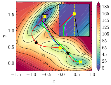
where we use the same set of parameters as in Ref. Müller and Brown 1979, namely: $\mbox{\boldmath$A$}=(-200,-100,-170,15)$ , $\mbox{\boldmath$a$}=(-1,-1,-6.5,0.7)$ , $\mbox{\boldmath$b$}=(0,0,11,0.6)$ , $\mbox{\boldmath$c$}=(-10,-10,-6.5,0.7)$ , $\mbox{\boldmath$x$}_{0}=(1,0,-0.5,-1)$ , and $\mbox{\boldmath$y$}_{0}=(0,0.5,1.5,1)$ .

The MEP follows the bent trajectory that goes through the critical points: two saddle points and one local minimum. This trajectory markedly differs from the LAPs, which are in a rough agreement. The MB surface highlights a problem with the DPM. As mentioned in Sec. III, the DPM can only search a single direction of each coordinate axis of the domain. In the case of the Muller-Brown surface, the DPM cannot search for trajectories bending back in the negative- $x$ direction. As seen in the inset of Fig. 4, the NEB, EL, and DA methods start their trajectories moving backwards in $x$ from the initial point $\mbox{\boldmath$q$}_{\textrm{in}}$ . The DPM path, on the other hand, always moves in the positive- $x$ direction. Consequently, the action integral along the DPM path is slightly larger than in the other methods.

IV.2 Realistic calculations

To illustrate the performance of the NEB method and other approaches to the LAP in realistic cases, we carried out nuclear EDF calculations for ²³²U in two collective coordinates and ²⁴⁰Pu in three collective coordinates. In the particle-hole channel we used the Skyrme functional SkM^∗ Bartel et al. 1982, which is often employed in fission studies. The particle-particle interaction was approximated by the mixed density-dependent pairing force Dobaczewski et al. 2002.

In the case of ²³²U, we considered two collective coordinates $\mbox{\boldmath$q$}\equiv(Q_{20},Q_{30})$ and for ²⁴⁰Pu we took three collective coordinates $\mbox{\boldmath$q$}\equiv(Q_{20},Q_{30},\lambda_{2})$ . The axial quadrupole and octupole moment operators are defined as in Ref. Dobaczewski and Olbratowski 2004:

\displaystyle\hat{Q}_{\lambda 0}(r,\theta)=\mathcal{N}_{\lambda}\sqrt{\frac{2\lambda+1}{4\pi}}r^{\lambda}P_{\lambda}(\cos\theta)

(19)

where $P_{\lambda}$ is the Legendre polynomial, $\mathcal{N}_{2}=\sqrt{\frac{16\pi}{5}}$ , and $\mathcal{N}_{3}=1$ . The collective coordinate $\lambda_{2}=\lambda_{2n}+\lambda_{2p}$ defined in Sec. II represents the dynamic pairing fluctuations. The value of $\lambda_{2\tau}$ = 0 corresponds to static HFB pairing.

As in Ref. Sadhukhan et al. 2014, to render collective coordinates dimensionless, we use dimensionless coordinates ${x_{i}}$ defined as

\displaystyle x_{i}

\displaystyle=

\displaystyle\frac{q_{i}}{\delta{q_{i}}},

(20)

where $\delta{q_{i}}$ are the scale parameters used in determining numerical derivatives of density matrices in Eq. (2). Here we took $\delta{Q_{20}}=1$ b, $\delta{Q_{30}}=1$ b^3/2 and $\delta{\lambda_{2}}=0.01$ MeV.

Two dimensional case: SF of ²³²U

The PES was computed by solving the HFB equations using the parallel axial solver HFBTHO(v3.00)Navarro Perez et al. 2017. The large stretched harmonic oscillator basis of $N=25$ major shells was used to guarantee good convergence. We adopted a $458\times 501$ grid with $0\leq Q_{20}\leq{457}$ b and $0\leq Q_{30}\leq{50}$ b^3/2. To apply the NEB method, which involves local gradient calculations at arbitrary values $q$ , we interpolate the PES and the inertia tensor on the mesh. Because the grid is two dimensional, a cubic spline interpolator suffices. Close to the $Q_{30}=0$ axis, we take into account the mirror symmetry of the PES by setting $V(-Q_{30})=V(Q_{30})$ . Finally, since NEB updates occasionally push an image outside of the computed PES mesh, we extended the PES to grow exponentially with the distance outside the mesh, to smoothly push images back into the evaluated region.

Figure 7: The PES of ²³²U in the

(Q_{20},Q_{30})

plane calculated with SkM^∗. Solid lines mark the LAPs and MEP obtained with the constant inertia tensor; dotted lines correspond to the non-perturbative inertia tensor. The OTL is shown in white. The blue, orange, purple and black curves represent the LAPs calculated using the NEB, DPM, EL, and DA methods, respectively. The green curve is the MEP, which was also calculated using NEB.

Figure 7 shows the two-dimensional PES of ²³²U. The least action fission pathway which goes from the g.s. at $\mbox{\boldmath$q$}_{\textrm{in}}$ =(24 b, 0) to the exit point $\mbox{\boldmath$q$}_{\textrm{fin}}$ =(281 b, 37 b^3/2) is calculated using the methods explained in Sec. III. To select the endpoint $\mbox{\boldmath$q$}_{\textrm{fin}}$ , we compute the LAP using DPM for all points on the OTL, and select the point with the lowest action integral. This point is then used as the exit point for the other methods. While NEB does not require a fixed endpoint in general, we fix the endpoint here in order to facilitate inter-method comparison. The MEP path is calculated using the NEB method.

The action integral computed with different methods is shown in Table 2. When computing the action, we interpolate the paths using a linear spline interpolator, and the action integral is computed using 500 evaluations along the path. This reduces the differences in the action that may arise from using a different number of points along the path (for instance, NEB gives a similar path to DPM using as few as 30 images). For all paths, we compute the action using the inertia tensor evaluated along the path. As can be seen, the action values computed for ²³²U using different methods agree well, with DA being the worst performer. As seen in Fig. 7 and Table 2 the MEP is very close to the LAP. This is because the static fission pathway (i.e., MEP) is fairly straight and the fission valley is well delineated. Note that perfect agreement is not expected, and in fact was not observed for the analytic surfaces, either. This is due in part to the different approximations used in each method — for DPM and DA, this is the grid spacing; for NEB, this is the number of images and approximate treatment of derivatives; and for EL, this is a variety of simplifications described in Sec. 3 in the SM SM. Additional variation in the quality of the interpolator further hampers agreement beyond what is listed.

Table 2: Action integrals for ²³²U computed with different methods. The paths computed using the constant and non-perturbative inertia tensor are labelled as “con.” and “n.-p.”, respectively.

		NEB-MEP	NEB-LAP	DPM	EL	DA
²³²U	con.	174.5	174.2	174.2	174.9	175.8
²³²U	n.-p.	-	173.6	173.3	175.0	178.5
²⁴⁰Pu	con.	19.09	18.98	19.21	19.01	22.85
²⁴⁰Pu	n.-p.	-	16.54	16.47	18.18	30.50

Three dimensional case: SF of ²⁴⁰Pu

The SF of ²⁴⁰Pu in several collective coordinates was studied in Ref. Sadhukhan et al. 2014 where the details pertaining to the computation, grid size, etc., can be found. Between the g.s. minimum and the fission isomer (FI), the fission pathway is affected by triaxial degrees of freedom. Between the FI and the outer turning surface (OTS), however, the predicted fission trajectory is axial. In this paper, we consider the fission of the FI of ²⁴⁰Pu so the OTS corresponds to the FI energy.

For three-dimensional tunneling, the system of equations that must be solved to construct a global spline interpolator is too large for practical applications. Instead, we use piecewise linear interpolation. The PES at $\lambda_{2}=0$ for ²⁴⁰Pu shown in Fig. 8 varies very smoothly in the barrier region where the potential energy is larger than the energy of the FI, and so this interpolation scheme is reasonable.

Figure 8: The PES for ²⁴⁰Pu in the space of collective coordinates

Q_{20}

Q_{30}

with

\lambda_{2}=0

. Only the region beyond the fission isomer is shown. The energy is normalized to the energy of the fission isomer. The OTL is shown in white. The MEP (green) practically coincides with the LAPs calculated with the constant inertia using the NEB (blue), DPM (orange), and EL (purple) methods.

Figure 9 shows the LAPs for ²⁴⁰Pu computed with the NEB, DPM, and EL methods in three dimensions (3D). The pathways begin at the FI minimum at $\mbox{\boldmath$q$}_{\textrm{in}}=(Q_{20}^{0}=87\,\text{b},Q_{30}^{0}=0\,\textrm{b}^{3/2},\lambda_{2}=0.0)$ and the exit point was chosen for DP in the same way as the ²³²U results before. The NEB endpoint in this case was allowed to vary according to Eq. 13, better representing standard procedure for production runs. The exit points $\mbox{\boldmath$q$}_{\textrm{fin}}$ predicted by NEB ( $185.1\,\text{b},18.4\,\text{b}^{3/2},3.3\,\text{MeV}$ ), DPM ( $184.0\,\text{b},18.6\,\text{b}^{3/2},4.8\,\text{MeV}$ ) and EL ( $179.8\,\text{b},17.7\,\text{b}^{3/2},0.0$ ) then differ. When the collective mass is held constant, all methods find very similar paths in the $\lambda_{2}=0.0$ plane, which are also shown in Fig. 8. The paths vary more when the non-perturbative inertia tensor is used, with the main difference between the NEB and DPM paths appearing in the region close to the FI minimum; beyond the saddle point, both paths are similar.

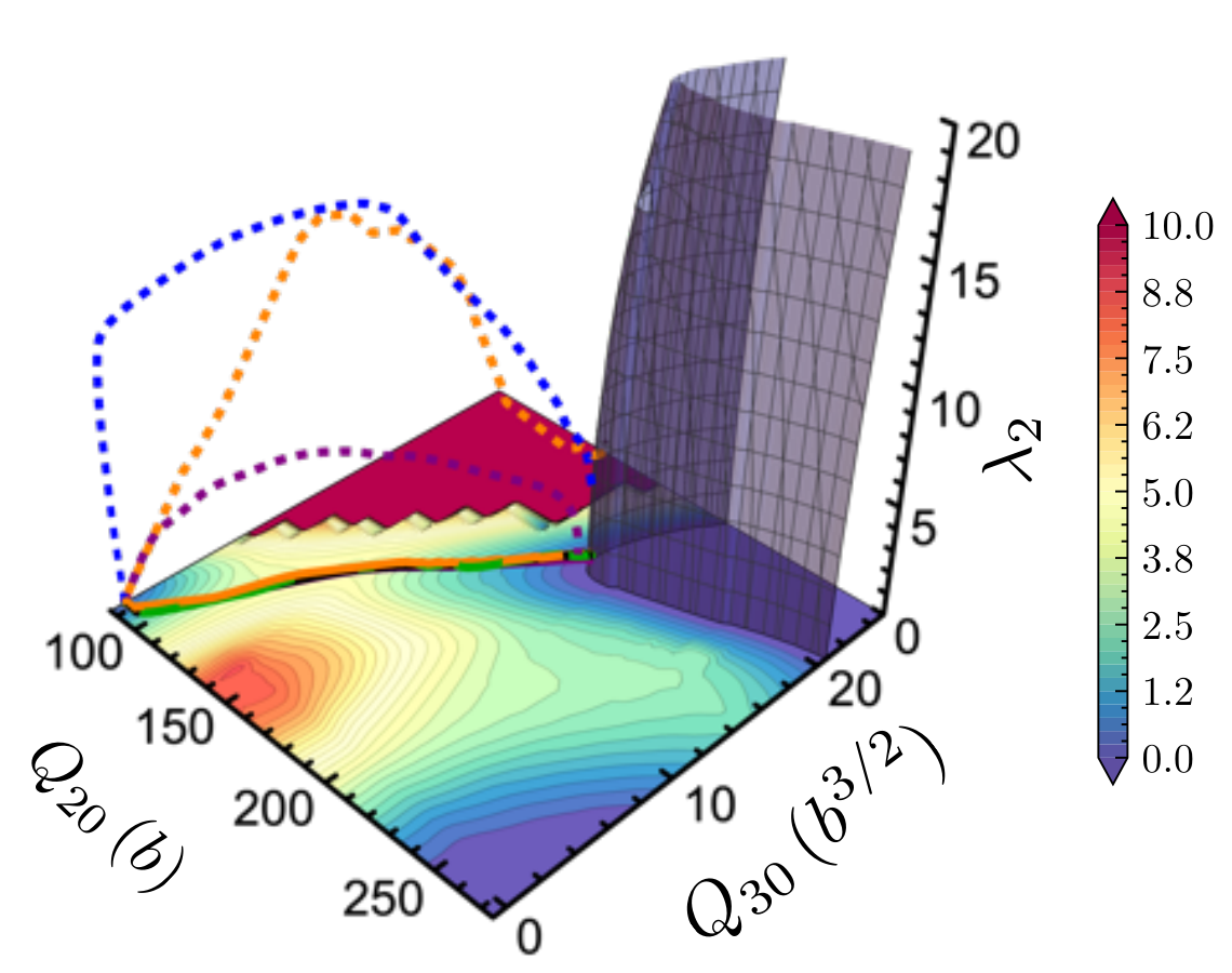
As seen in Table 2, the NEB and DPM are in a good agreement. In general, one would expect a better performance from NEB as this method is not constrained to a grid (this is true in the case of the analytic surfaces discussed in Sec. IV.1). However, in rare cases, the DPM produces a slightly lower action than the NEB. In such cases the NEB converges to an even lower action if is initialized with the DPM result. This suggests that for tunneling in more than 2D, a combination of NEB and DPM might be beneficial.

V Conclusions

Finding the path that minimizes the action integral can be extremely challenging since it involves searching over the space of all continuous paths that fulfill the boundary conditions. Each method explored in this paper simplifies such task in different ways. DPM and DA project the PES onto a finite grid and explore decisions in making the path between the boundary conditions. In the EL approach the surface is modified in several ways to smooth the relation between initial conditions and the end point of the trajectory. The NEB method reduces the original search over continuous path into considering only piece-wise linear paths, the number of pieces given by the number of images. It is this simplification that makes the NEB robust and accurate, since the total action now becomes a smooth function of the position of the images, a function that can straightforwardly be numerically minimized by gradient descent methods.

A significant advantage of the NEB is that it can accommodate any initial positions of the images, which speeds the convergence appreciably if a good prior guess of the LAP is provided. Other methods lack for such incorporation of prior knowledge. Finally, the resolution of the NEB for a rapidly varying surface can be adjusted locally by increasing the amount of images or spring constants, while for DPM and DA the entire grid resolution would have to be increased, giving an appreciable toll on the computational cost.

For both analytic and realistic potential energy surfaces the NEB robustly produces a LAP. In the cases studied, NEB outperforms the EL and DA methods, and produces close results to those of the DPM with usually lower action integral. For many-dimensional tunneling, initiating the NEB method from the DPM path might be a winning strategy.

A huge advantage of the NEB over other methods is that it can efficiently and accurately estimate exit points. By exploring different initial conditions for the positions of the images which lead to distinct exit points, one can use the NEB method to study the phenomenon of multimodal fission. An example of such an application is shown in video 1 in the SM SM. Whilst other methods can find a least-action trajectory for an arbitrary final point placed on the OTL, as done, e.g., in Refs. Sadhukhan et al. 2013; Sadhukhan et al. 2014; Sadhukhan et al. 2016; Sadhukhan et al. 2017; Zhao et al. 2015; Zhao et al. 2016; Mercier et al. 2021, they cannot guarantee that this trajectory is stationary. All such trajectories can be gradually transformed into a stationary pathway by moving the final point along the OTL towards the exit point, see Fig. 2.

In this paper we also explored the minimum-energy (or static) path. We adjusted our NEB algorithm to generate MEPs, including the determination of local minima and saddle points. The necessary conditions for an MEP to also be an LAP are discussed in the SM SM. Video 2 in the SM SM illustrates the way the NEB method generates LAP and MEP.

An important contribution of this work is providing a beta release of the PyNEB package, a python suite of codes that implement the NEB algorithm described in this paper. The package can be found in PyN together with the respective documentation and code samples serving as a tutorial for its use. A comprehensive investigation into the intricacies of the numerical implementations and performance of the package itself will accompany the version $1.0$ release.

The NEB approach can be readily paired with accelerated DFT calculations, such as the recent applications of Gaussian process regression to PES emulation Koistinen et al. 2017; Garrido Torres et al. 2019. In these works, a Gaussian process is used to emulate the PES and DFT calculations are only run if the Gaussian process is uncertain as to the actual PES value. As NEB is not a grid-based method, it can sensibly be paired with a Gaussian process emulator that is updated as necessary while NEB runs. In this way, the LAP can be determined using far fewer DFT evaluations than is necessary in DPM.

The ability to determine the exit points is essential for determining fission fragment yields Sadhukhan et al. 2020; Sadhukhan et al. 2022. The minimum action provides information on SF half-lives. In this context, the NEB method described in this paper is expected to speed up the global calculations of nuclear fission for r-process simulations and studies of superheavy nuclei stability.

$\bullet$

Acknowledgements.

We are grateful to Edgard Bonilla and Stefan M. Wild for useful comments. This work was supported by the U.S. Department of Energy under Award Numbers DOE-DE-NA0002847 (NNSA, the Stewardship Science Academic Alliances program), DE-SC0013365 (Office of Science), and DE-SC0018083 (Office of Science, NUCLEI SciDAC-4 collaboration) and by the National Science Foundation CSSI program under award number 2004601 (BAND collaboration).

E.F. and D.L. contributed equally to this work.

References

Krappe and Pomorski (2012) H. J. Krappe and K. Pomorski, Theory of Nuclear Fission, Lecture Notes in Physics 838 (Springer Verlag, Heidelberg, 2012).
Schmidt and Jurado (2018) K. H. Schmidt and B. Jurado, “Review on the progress in nuclear fission: experimental methods and theoretical descriptions,” Rep. Prog. Phys. 81, 106301 (2018).
Giuliani et al. (2019) S. A. Giuliani, Z. Matheson, W. Nazarewicz, E. Olsen, P.-G. Reinhard, J. Sadhukhan, B. Schuetrumpf, N. Schunck, and P. Schwerdtfeger, “Colloquium: Superheavy elements: Oganesson and beyond,” Rev. Mod. Phys. 91, 011001 (2019).
Vogel et al. (2015) P. Vogel, L. Wen, and C. Zhang, “Neutrino oscillation studies with reactors,” Nat. Commun. 6, 6935 (2015).
Horowitz et al. (2019) C. J. Horowitz, A. Arcones, B. Côté, I. Dillmann, W. Nazarewicz, I. U. Roederer, H. Schatz, A. Aprahamian, D. Atanasov, A. Bauswein, T. C. Beers, J. Bliss, M. Brodeur, J. A. Clark, A. Frebel, F. Foucart, C. J. Hansen, O. Just, A. Kankainen, G. C. McLaughlin, J. M. Kelly, S. N. Liddick, D. M. Lee, J. Lippuner, D. Martin, J. Mendoza-Temis, B. D. Metzger, M. R. Mumpower, G. Perdikakis, J. Pereira, B. W. O’Shea, R. Reifarth, A. M. Rogers, D. M. Siegel, A. Spyrou, R. Surman, X. Tang, T. Uesaka, and M. Wang, “R-process nucleosynthesis: connecting rare-isotope beam facilities with the cosmos,” J. Phys. G 46, 083001 (2019).
Vassh et al. (2019) N. Vassh, R. Vogt, R. Surman, J. Randrup, T. M. Sprouse, M. R. Mumpower, P. Jaffke, D. Shaw, E. M. Holmbeck, Y.-L. Zhu, and G. C. McLaughlin, “Using excitation-energy dependent fission yields to identify key fissioning nuclei in r -process nucleosynthesis,” J. Phys. G 46, 065202 (2019).
Giuliani et al. (2020) S. A. Giuliani, G. Martínez-Pinedo, M.-R. Wu, and L. M. Robledo, “Fission and the $r$ -process nucleosynthesis of translead nuclei in neutron star mergers,” Phys. Rev. C 102, 045804 (2020).
Schunck and Robledo (2016) N. Schunck and L. M. Robledo, “Microscopic theory of nuclear fission: a review,” Rep. Prog. Phys. 79, 116301 (2016).
Bender et al. (2020) M. Bender, R. Bernard, G. Bertsch, S. Chiba, J. Dobaczewski, N. Dubray, S. A. Giuliani, K. Hagino, D. Lacroix, Z. Li, P. Magierski, J. Maruhn, W. Nazarewicz, J. Pei, S. Péru, N. Pillet, J. Randrup, D. Regnier, P.-G. Reinhard, L. M. Robledo, W. Ryssens, J. Sadhukhan, G. Scamps, N. Schunck, C. Simenel, J. Skalski, I. Stetcu, P. Stevenson, S. Umar, M. Verriere, D. Vretenar, M. Warda, and S. Åberg, “Future of nuclear fission theory,” J. Phys. G 47, 113002 (2020).
Bender et al. (2003) M. Bender, P.-H. Heenen, and P.-G. Reinhard, “Self-consistent mean-field models for nuclear structure,” Rev. Mod. Phys. 75, 121–180 (2003).
Schunck (2019) N. Schunck, Energy density functional methods for atomic nuclei, IOP Expanding Physics (IOP Publishing, Bristol, UK, 2019).
Kapur and Peierls (1937) P. L. Kapur and R. Peierls, “Penetration into potential barriers in several dimensions,” Proc. R. Soc. A 163, 606–610 (1937).
Brack et al. (1972) M. Brack, J. Damgaard, A. S. Jensen, H. C. Pauli, V. M. Strutinsky, and C. Y. Wong, “Funny Hills: The shell-correction approach to nuclear shell effects and its applications to the fission process,” Rev. Mod. Phys. 44, 320–405 (1972).
Ledergerber and Pauli (1973) T. Ledergerber and H.-C. Pauli, “On the dynamics of fission: The role of reflection asymmetry in the nuclear shape,” Nucl. Phys. A 207, 1–32 (1973).
Baran et al. (1981) A. Baran, K. Pomorski, A. Lukasiak, and A. Sobiczewski, “A dynamic analysis of spontaneous-fission half-lives,” Nucl. Phys. A 361, 83 (1981).
Baran (1978) A. Baran, “Some dynamical aspects of the fission process,” Phys. Lett. B 76, 8 – 10 (1978).
Sadhukhan et al. (2013) J. Sadhukhan, K. Mazurek, A. Baran, J. Dobaczewski, W. Nazarewicz, and J. A. Sheikh, “Spontaneous fission lifetimes from the minimization of self-consistent collective action,” Phys. Rev. C 88, 064314 (2013).
Sadhukhan et al. (2014) J. Sadhukhan, J. Dobaczewski, W. Nazarewicz, J. A. Sheikh, and A. Baran, “Pairing-induced speedup of nuclear spontaneous fission,” Phys. Rev. C 90, 061304 (2014).
Sadhukhan et al. (2016) J. Sadhukhan, W. Nazarewicz, and N. Schunck, “Microscopic modeling of mass and charge distributions in the spontaneous fission of ${}^{240}\mathrm{Pu}$ ,” Phys. Rev. C 93, 011304 (2016).
Sadhukhan et al. (2017) J. Sadhukhan, C. Zhang, W. Nazarewicz, and N. Schunck, “Formation and distribution of fragments in the spontaneous fission of ²⁴⁰Pu,” Phys. Rev. C 96, 061301 (2017).
Zhao et al. (2015) J. Zhao, B.-N. Lu, T. Nikšić, and D. Vretenar, “Multidimensionally constrained relativistic Hartree-Bogoliubov study of spontaneous nuclear fission,” Phys. Rev. C 92, 064315 (2015).
Zhao et al. (2016) J. Zhao, B.-N. Lu, T. Nikšić, D. Vretenar, and S.-G. Zhou, “Multidimensionally-constrained relativistic mean-field study of spontaneous fission: Coupling between shape and pairing degrees of freedom,” Phys. Rev. C 93, 044315 (2016).
Mercier et al. (2021) F. Mercier, J. Zhao, J.-P. Ebran, E. Khan, T. Nikšić, and D. Vretenar, “Microscopic description of $2\alpha$ decay in ${}^{212}\mathrm{Po}$ and ${}^{224}\mathrm{Ra}$ isotopes,” Phys. Rev. Lett. 127, 012501 (2021).
Schmid (1986) A. Schmid, “Quasiclassical wave function in multidimensional quantum decay problems,” Ann. Phys. (NY) 170, 333–369 (1986).
Eckern and Schmid (1992) U. Eckern and A. Schmid, “Chapter 3 - the decay of a metastable state in a multidimensional configuration space,” in Quantum Tunnelling in Condensed Media, Modern Problems in Condensed Matter Sciences, Vol. 34, edited by Y. Kagan and A. Leggett (Elsevier, 1992) pp. 145–229.
Kindo and Iwamoto (1989) T. Kindo and A. Iwamoto, “Methods for the calculation of the fission half-life in the multi-dimensional space,” Phys. Lett. B 225, 203–207 (1989).
Iwamoto and Tomita (1992) A. Iwamoto and Y. Tomita, “Adiabatic approximation in multi-dimensional penetration problem,” Prog. Theor. Phys. 87, 1171–1184 (1992).
Iwamoto (1994) A. Iwamoto, “Multi-dimensional tunneling and nuclear fission process,” Z. Phys. A 349, 265 (1994).
Scamps and Hagino (2015) G. Scamps and K. Hagino, “Multidimensional fission model with a complex absorbing potential,” Phys. Rev. C 91, 044606 (2015).
Garrett and Truhlar (1983) B. C. Garrett and D. G. Truhlar, “A least-action variational method for calculating multidimensional tunneling probabilities for chemical reactions,” J. Chem. Phys. 79, 4931–4938 (1983).
Mills and Jónsson (1994) G. Mills and H. Jónsson, “Quantum and thermal effects in H₂ dissociative adsorption: Evaluation of free energy barriers in multidimensional quantum systems,” Phys. Rev. Lett. 72, 1124–1127 (1994).
Mills et al. (1995) G. Mills, H. Jónsson, and G. K. Schenter, “Reversible work transition state theory: application to dissociative adsorption of hydrogen,” Surf. Sci. 324, 305–337 (1995).
(33) H. Jónsson, G. Mills, and K. W. Jacobsen, “Nudged elastic band method for finding minimum energy paths of transitions,” in Classical and Quantum Dynamics in Condensed Phase Simulations, pp. 385–404.
Henkelman et al. (2000) G. Henkelman, B. P. Uberuaga, and H. Jónsson, “A climbing image nudged elastic band method for finding saddle points and minimum energy paths,” J. Chem. Phys. 113, 9901–9904 (2000).
Henkelman and Jónsson (2000) G. Henkelman and H. Jónsson, “Improved tangent estimate in the nudged elastic band method for finding minimum energy paths and saddle points,” J. Chem. Phys. 113, 9978–9985 (2000).
(36) “The Atomic Simulation Environment Documentation,” https://wiki.fysik.dtu.dk/ase/ase/neb.html.
Peters et al. (2004) B. Peters, A. Heyden, A. T. Bell, and A. Chakraborty, “A growing string method for determining transition states: Comparison to the nudged elastic band and string methods,” J. Chem. Phys. 120, 7877–7886 (2004).
Mamdouh et al. (1998) A. Mamdouh, J. Pearson, M. Rayet, and F. Tondeur, “Large-scale fission-barrier calculations with the ETFSI method,” Nucl. Phys. A 644, 389–414 (1998).
Möller et al. (2001) P. Möller, D. G. Madland, A. J. Sierk, and A. Iwamoto, “Nuclear fission modes and fragment mass asymmetries in a five-dimensional deformation space,” Nature 409, 785–790 (2001).
Iwamoto et al. (2002) A. Iwamoto, P. Möller, D. G. Madland, and A. J. Sierk, “Mass division in nuclear fission and isotope effect,” J. Nucl. Sci. Technol. 39, 332–336 (2002).
Möller et al. (2004) P. Möller, A. J. Sierk, and A. Iwamoto, “Five-dimensional fission-barrier calculations from ${}^{70}\mathrm{S}\mathrm{e}$ to ${}^{252}\mathrm{C}\mathrm{f}$ ,” Phys. Rev. Lett. 92, 072501 (2004).
Wang et al. (2019) Z.-M. Wang, W.-J. Zhu, X. Zhu, C.-L. Zhong, and T.-S. Fan, “²³⁶U multi-modal fission paths on a five-dimensional deformation surface,” Commun. Theor. Phys. 71, 417 (2019).
Ásgeirsson et al. (2021) V. Ásgeirsson, B. O. Birgisson, R. Bjornsson, U. Becker, F. Neese, C. Riplinger, and H. Jónsson, “Nudged elastic band method for molecular reactions using energy-weighted springs combined with eigenvector following,” J. Chem. Theory Comput. (2021), 10.1021/acs.jctc.1c00462.
Sheppard et al. (2008) D. Sheppard, R. Terrell, and G. Henkelman, “Optimization methods for finding minimum energy paths,” J. Chem. Phys. 128, 134106 (2008).
Moré and Munson (2004) J. J. Moré and T. S. Munson, “Computing mountain passes and transition states,” Math. Program. 100, 151–182 (2004).
Vaquero et al. (2011) N. L. Vaquero, T. R. Rodríguez, and J. L. Egido, “On the impact of large amplitude pairing fluctuations on nuclear spectra,” Phys. Lett. B 704, 520 – 526 (2011).
Vaquero et al. (2013) N. L. Vaquero, J. L. Egido, and T. R. Rodríguez, “Large-amplitude pairing fluctuations in atomic nuclei,” Phys. Rev. C 88, 064311 (2013).
Warda et al. (2012) M. Warda, A. Staszczak, and W. Nazarewicz, “Fission modes of mercury isotopes,” Phys. Rev. C 86, 024601 (2012).
Berger et al. (1984) J. Berger, M. Girod, and D. Gogny, “Microscopic analysis of collective dynamics in low energy fission,” Nucl. Phys. A 428, 23–36 (1984).
Sadhukhan et al. (2020) J. Sadhukhan, S. A. Giuliani, Z. Matheson, and W. Nazarewicz, “Efficient method for estimation of fission fragment yields of $r$ -process nuclei,” Phys. Rev. C 101, 065803 (2020).
Sadhukhan et al. (2022) J. Sadhukhan, S. A. Giuliani, and W. Nazarewicz, “Theoretical description of fission yields: Toward a fast and efficient global model,” Phys. Rev. C 105, 014619 (2022).
Baran et al. (2011) A. Baran, J. A. Sheikh, J. Dobaczewski, W. Nazarewicz, and A. Staszczak, “Quadrupole collective inertia in nuclear fission: Cranking approximation,” Phys. Rev. C 84, 054321 (2011).
Giuliani and Robledo (2018) S. A. Giuliani and L. M. Robledo, “Non-perturbative collective inertias for fission: A comparative study,” Phys. Lett. B 787, 134–140 (2018).
Washiyama et al. (2021) K. Washiyama, N. Hinohara, and T. Nakatsukasa, “Finite-amplitude method for collective inertia in spontaneous fission,” Phys. Rev. C 103, 014306 (2021).
Baran et al. (2005) A. Baran, Z. Łojewski, K. Sieja, and M. Kowal, “Global properties of even-even superheavy nuclei in macroscopic-microscopic models,” Phys. Rev. C 72, 044310 (2005).
Quapp and Heidrich (1984) W. Quapp and D. Heidrich, “Analysis of the concept of minimum energy path on the potential energy surface of chemically reacting systems,” Theoret. Chim. Acta. 66, 245–260 (1984).
Dubray and Regnier (2012) N. Dubray and D. Regnier, “Numerical search of discontinuities in self-consistent potential energy surfaces,” Comput. Phys. Commun. 183, 2035–2041 (2012).
Zdeb et al. (2021) A. Zdeb, M. Warda, and L. M. Robledo, “Description of the multidimensional potential-energy surface in fission of ${}^{252}\mathrm{Cf}$ and ${}^{258}\mathrm{No}$ ,” Phys. Rev. C 104, 014610 (2021).
Lau et al. (2021) N. W. T. Lau, R. N. Bernard, and C. Simenel, “Smoothing of 1D and 2D discontinuities in potential energy surfaces,” (2021), arXiv:2111.06513 [nucl-th] .
(60) See Supplemental Material at (link) for the algorithms, videos, and details on MEP and LAP equivalence conditions, and the Euler-Lagrange implementation.
(61) https://pyneb.dev.
Ásgeirsson et al. (2018) V. Ásgeirsson, A. Arnaldsson, and H. Jónsson, “Efficient evaluation of atom tunneling combined with electronic structure calculations,” J. Chem. Phys. 148, 102334 (2018).
Verlet (1967) L. Verlet, “Computer "experiments" on classical fluids. I. thermodynamical properties of Lennard-Jones molecules,” Phys. Rev. 159, 98–103 (1967).
Bitzek et al. (2006) E. Bitzek, P. Koskinen, F. Gähler, M. Moseler, and P. Gumbsch, “Structural relaxation made simple,” Phys. Rev. Lett. 97, 170201 (2006).
Guénolé et al. (2020) J. Guénolé, W. G. Nöhring, A. Vaid, F. Houllé, Z. Xie, A. Prakash, and E. Bitzek, “Assessment and optimization of the fast inertial relaxation engine (FIRE) for energy minimization in atomistic simulations and its implementation in LAMMPS,” Comput. Mater. Sci. 175, 109584 (2020).
Dijkstra (1959) E. W. Dijkstra, “A note on two problems in connexion with graphs,” Numer. Math. 1, 269–271 (1959).
Weinstock (1974) R. Weinstock, Calculus of variations: with applications to physics and engineering (Courier Corporation, 1974).
(68) “Numerical Solution of Boundary Value Problems (BVP),” https://reference.wolfram.com/language/tutorial/NDSolveBVP.html.
Lakshminarayanan and Varadharajan (1997) V. Lakshminarayanan and S. Varadharajan, “Dynamic programming, the Fermat principle, and the eikonal equation revisited,” J. Optim. Theory Appl. 95, 713–716 (1997).
Müller and Brown (1979) K. Müller and L. D. Brown, “Location of saddle points and minimum energy paths by a constrained simplex optimization procedure,” Theoret. Chim. Acta. 53, 75–93 (1979).
Koistinen et al. (2017) O.-P. Koistinen, F. B. Dagbjartsdóttir, V. Ásgeirsson, A. Vehtari, and H. Jónsson, “Nudged elastic band calculations accelerated with Gaussian process regression,” J. Chem. Phys. 147, 152720 (2017).
Bartel et al. (1982) J. Bartel, P. Quentin, M. Brack, C. Guet, and H.-B. Håkansson, “Towards a better parametrisation of skyrme-like effective forces: A critical study of the skm force,” Nucl. Phys. A 386, 79–100 (1982).
Dobaczewski et al. (2002) J. Dobaczewski, W. Nazarewicz, and M. V. Stoitsov, “Nuclear ground-state properties from mean-field calculations,” Eur. Phys. J. A 15, 21–26 (2002).
Dobaczewski and Olbratowski (2004) J. Dobaczewski and P. Olbratowski, “Solution of the Skyrme–Hartree–Fock–Bogolyubov equations in the Cartesian deformed harmonic-oscillator basis. (IV) HFODD (v2.08i): a new version of the program,” Comput. Phys. Commun. 158, 158–191 (2004).
Navarro Perez et al. (2017) R. Navarro Perez, N. Schunck, R.-D. Lasseri, C. Zhang, and J. Sarich, “Axially deformed solution of the Skyrme–Hartree–Fock–Bogolyubov equations using the transformed harmonic oscillator basis (III) HFBTHO (v3.00): A new version of the program,” Comput. Phys. Commun. 220, 363–375 (2017).
Garrido Torres et al. (2019) J. A. Garrido Torres, P. C. Jennings, M. H. Hansen, J. R. Boes, and T. Bligaard, “Low-scaling algorithm for nudged elastic band calculations using a surrogate machine learning model,” Phys. Rev. Lett. 122, 156001 (2019).