跳到论文正文
W Papers独立论文阅读器 arXiv:2203.01497 论文正文 计算阅读时间 · 0%
引用这篇论文根据当前论文元数据生成,正式投稿前建议核对。


License: arXiv.org perpetual non-exclusive license
arXiv:2203.01497v2 [cs.RO] 14 Aug 2022

Analytical Second-Order Partial Derivatives of Rigid-Body Inverse Dynamics

Shubham Singh Affiliation:  Aerospace Engineering, The University of Texas at Austin, TX-78751, USA. singh281@utexas.edu, ryan.russell@utexas.edu     Ryan P. Russell Affiliation:  Aerospace Engineering, The University of Texas at Austin, TX-78751, USA. singh281@utexas.edu, ryan.russell@utexas.edu     Patrick M. Wensing Thanks: This work was supported in part by the National Science Foundation grants CMMI-1835013 and CMMI-1835186. Affiliation:  Aerospace & Mechanical Engineering, University of Notre Dame, IN-46556, USA. pwensing@nd.edu
Abstract

Optimization-based robot control strategies often rely on first-order dynamics approximation methods, as in iLQR. Using second-order approximations of the dynamics is expensive due to the costly second-order partial derivatives of the dynamics with respect to the state and control. Current approaches for calculating these derivatives typically use automatic differentiation (AD) and chain-rule accumulation or finite-difference. In this paper, for the first time, we present analytical expressions for the second-order partial derivatives of inverse dynamics for open-chain rigid-body systems with floating base and multi-DoF joints. A new extension of spatial vector algebra is proposed that enables the analysis. A recursive algorithm with complexity of 𝒪⁡(N​d2)\mathcal{O}(Nd^{2}) is also provided where NN is the number of bodies and dd is the depth of the kinematic tree. A comparison with AD in CasADi shows speedups of 1.5-3×\times for serial kinematic trees with N>5N>5, and a C++ implementation shows runtimes of ≈\approx51μ​s\mu s for a quadruped.

I Introduction

In recent years, optimization-based methods have become popular for robot motion generation and control. Although full second-order (SO) optimization methods offer superior convergence properties, most work has focused on using only the first-order (FO) dynamics approximation, such as in iLQR [1, 2]. Differential Dynamic Programming (DDP) [3] is a use-case for full SO optimization that has gained wide interest for robotics applications [4, 5, 6, 7]. Variants of DDP using multiple shooting [8] and parallelization [9] have been developed for computational and numerical improvements.

The state-of-the-art for including SO dynamics derivatives in trajectory optimization is the work by Lee et al. [10], where they use forward chain-rule expressions (i.e., recursive derivative expressions) to calculate the SO partial derivatives of joint torques with respect to joint configuration and joint rates for revolute and prismatic joint models. Nganga and Wensing [11] presented a method for getting the SO directional derivatives of inverse dynamics as needed in the backward pass of DDP by employing reverse mode Automatic Differentiation (AD) and a modified version of the Recursive Newton Euler Algorithm (RNEA) [12]. Although this strategy avoids the need for the full SO partial derivatives of RNEA, it lacks the opportunity for parallel computation across the trajectory. Full SO partial derivatives calculation, on the other hand, can be easily parallelized to accelerate the backward pass of DDP. Other trajectory optimization schemes aside from DDP may also benefit from the full SO partials.

AD tools depend on forward or reverse chain-rule accumulation and can suffer from high memory requirements [13]. Finite-difference methods, on the other hand, can be parallelized, but suffer from low accuracy. Such inaccurate Jacobian and Hessian approximations during optimization often lead to ill-conditioning, and poor convergence [10].

Although significant work has been done for computing FO partial derivatives of inverse/forward dynamics [14, 15, 16, 17], the literature still lacks analytical SO partial derivatives of rigid-body dynamics. This is mainly due to the tensor nature of SO derivatives, and the lack of established tools for working with dynamics tensors. The main contribution of this paper is to extend the FO derivatives of inverse dynamics (ID) presented in Ref. [14] to SO derivatives w.r.t the joint configuration (𝒒\boldsymbol{q}), velocity vector (𝒒˙\dot{\boldsymbol{q}}), and joint acceleration (𝒒¨\ddot{\boldsymbol{q}}) for multi-Degree-of-Freedom (DoF) joints modeled with Lie groups. Our method departs from the chain-rule approach used in [10], and thus gains additional efficiency in the associated algorithm. For this purpose, we contribute an extension of Featherstone’s spatial vector algebra tools [12] for tensor use. The SO derivatives algorithm herein could also be parallelized (e.g., for use with GPUs), building on the FO case in Ref. [18].

In the following sections, Spatial Vector Algebra (SVA) is reviewed for dynamics analysis, followed by an extension of SVA for use with second-order derivative tensors. Then, the algorithm is developed for the SO partial derivatives of ID. The resulting expressions and algorithm are very complicated, but are provided in the form of open-source algorithm, with full derivation in Ref. [19] while keeping the current paper self-contained. The performance of this new SO algorithm is compared to AD using CasADi [20] in Matlab.

II Rigid-Body Dynamics Background

Rigid-Body Dynamics: For a rigid-body system with nn-dimensional configuration manifold 𝒬\mathcal{Q}, the state variables are the configuration 𝒒∈𝒬\boldsymbol{q}\in\mathcal{Q} and the generalized velocity vector 𝒒˙∈ℝn\dot{\boldsymbol{q}}\in\mathbb{R}^{n}, while the control variable is the generalized force/torque vector 𝝉∈ℝn\boldsymbol{\tau}\in\mathbb{R}^{n}. With this convention, 𝒒˙\dot{\boldsymbol{q}} uniquely specifies the time rate of change for 𝒒\boldsymbol{q} without strictly being its time derivative. The Inverse Dynamics (ID), is given by

𝝉\displaystyle\boldsymbol{\tau} =𝑴⁡(𝒒)​𝒒¨+𝑪⁡(𝒒,𝒒˙)​𝒒˙+𝒈⁡(𝒒)\displaystyle=\boldsymbol{M}(\boldsymbol{q})\ddot{\boldsymbol{q}}+\boldsymbol{C}(\boldsymbol{q},\dot{\boldsymbol{q}})\dot{\boldsymbol{q}}+\boldsymbol{g}(\boldsymbol{q}) (1)
=ID​(model,𝒒,𝒒˙,𝒒¨)\displaystyle=\textrm{ID}({\rm model},\boldsymbol{q},\dot{\boldsymbol{q}},\ddot{\boldsymbol{q}}) (2)

where 𝑴∈ℝn×n\boldsymbol{M}\in\mathbb{R}^{n\times n} is the mass matrix, 𝑪∈ℝn×n\boldsymbol{C}\in\mathbb{R}^{n\times n} is the Coriolis matrix, and 𝒈∈ℝn\boldsymbol{g}\in\mathbb{R}^{n} is the vector of generalized gravitational forces. An efficient 𝒪⁡(N)\mathcal{O}(N) algorithm for ID is the RNEA [21, 12].

Notation: Spatial vectors are 6D vectors that combine the linear and angular aspects of a rigid-body motion or net force [12]. Cartesian vectors are denoted with lower-case letters with a bar (v¯\bar{v}), spatial vectors with lower-case bold letters (e.g., 𝒂\boldsymbol{a}), matrices with capitalized bold letters (e.g., 𝑨\boldsymbol{A}), and tensors with capitalized calligraphic letters (e.g., 𝒜\mathcal{A}). Motion vectors, such as velocity and acceleration, belong to a 6D vector space denoted M6M^{6}. Force-like vectors, such as force and momentum, belong to another 6D vector space F6F^{6}. Spatial vectors are usually expressed in either the ground coordinate frame or a body coordinate (local) frame. For example, the spatial velocity 𝒗kk∈M6{}^{k}\boldsymbol{v}_{k}\in M^{6} of a body kk expressed in the body frame is 𝒗kk=[ω¯⊤kkv¯⊤kk]⊤{}^{k}\boldsymbol{v}_{k}=\begin{bmatrix}{}^{k}\bar{\omega}_{k}^{\top}&{}^{k}\bar{v}_{k}^{\top}\end{bmatrix}^{\top} where ω¯kk{}^{k}\bar{\omega}_{k} ∈ℝ3\in\mathbb{R}^{3} is the angular velocity expressed in a coordinate frame fixed to the body, while v¯kk{}^{k}\bar{v}_{k} ∈ℝ3\in\mathbb{R}^{3} is the linear velocity of the origin of the body frame. When the frame used to express a spatial vector is omitted, the ground frame is assumed.

A spatial cross product between motion vectors (𝒗\boldsymbol{v},𝒖\boldsymbol{u}), written as (𝒗×)𝒖(\boldsymbol{v}\times)\boldsymbol{u}, is given by Eq. 3. This operation gives the time rate of change of 𝒖\boldsymbol{u}, when 𝒖\boldsymbol{u} is moving with a spatial velocity 𝒗\boldsymbol{v}. For a Cartesian vector ω¯\bar{\omega}, ω¯×\bar{\omega}\times is the 3D cross-product matrix. A spatial cross product between a motion and a force vector is written as (𝒗×∗)𝒇(\boldsymbol{v}\times^{*})\boldsymbol{f}, as defined by Eq. 4.

𝒗×=[ω¯×𝟎v¯×ω¯×]\displaystyle\boldsymbol{v}\times=\begin{bmatrix}\bar{\omega}\times&\bf{0}\\ \bar{v}\times&\bar{\omega}\times\end{bmatrix} (3)
𝒗×∗=[ω¯×v¯×𝟎ω¯×]\displaystyle\boldsymbol{v}\times^{*}=\begin{bmatrix}\bar{\omega}\times&\bar{v}\times\\ \bf{0}&\bar{\omega}\times\end{bmatrix} (4)

An operator ׯ∗\,\overline{\!\times\!}{}^{\,*} is defined by swapping the order of the cross product, such that (𝒇ׯ)∗𝒗=(𝒗×∗)𝒇(\boldsymbol{f}\,\overline{\!\times\!}{}^{\,*})\boldsymbol{v}=(\boldsymbol{v}\times^{*})\boldsymbol{f} [22]. Further introduction to SVA is provided in Ref. [12].

Connectivity: An open-chain kinematic tree (Fig. 1) is considered with NN links connected by joints, each with up to 6 DoF. Body ii’s parent toward the root of the tree is denoted as λ⁡(i)\lambda(i), and we define i⪯ji\preceq j if body ii is in the path from body jj to the root. Joint ii is defined as the connection between body ii and its predecessor.

We consider joints whose configurations form a sub-group of the Lie group SE(3). For a prismatic joint, the configuration and rate are represented by 𝒒i,𝒒˙i∈ℝ\boldsymbol{q}_{i},\dot{\boldsymbol{q}}_{i}\in\mathbb{R}, while for a revolute joint, 𝒒i∈S​O​(2)\boldsymbol{q}_{i}\in SO(2), and 𝒒˙i∈ℝ\dot{\boldsymbol{q}}_{i}\in\mathbb{R} gives the rotational rate of the joint. For a spherical joint, 𝒒i∈S​O​(3)\boldsymbol{q}_{i}\in SO(3), and 𝒒˙i=ω¯i/λ⁡(i)i∈ℝ3\dot{\boldsymbol{q}}_{i}={}^{i}\bar{\omega}_{i/\lambda(i)}\in\mathbb{R}^{3} gives relative angular velocity between neighboring bodies. For a 6-DoF free motion joint, 𝒒i∈S​E​(3)\boldsymbol{q}_{i}\in SE(3), and 𝒒˙i=𝒗i/λ⁡(i)i∈ℝ6\dot{\boldsymbol{q}}_{i}={}^{i}\boldsymbol{v}_{i/\lambda(i)}\in\mathbb{R}^{6}.

The spatial velocities of the neighbouring bodies in the tree are then related by the recursive expression 𝒗i=𝒗λ⁡(i)+𝑺i​𝒒˙i\boldsymbol{v}_{i}=\boldsymbol{v}_{\lambda(i)}+\boldsymbol{S}_{i}\dot{\boldsymbol{q}}_{i}, where 𝑺i∈ℝ6×ni\boldsymbol{S}_{i}\in\mathbb{R}^{6\times n_{i}} is the joint motion subspace matrix for joint ii [12] with nin_{i} its number of DoFs. The velocity 𝒗i\boldsymbol{v}_{i} can also be written in an analytical form as the sum of joint velocities over predecessors as 𝒗i=∑l⪯i𝑺l​𝒒˙l\boldsymbol{v}_{i}=\sum_{l\preceq i}\boldsymbol{S}_{l}\dot{\boldsymbol{q}}_{l}. The derivative of the joint motion subspace matrix in local coordinates (often denoted 𝑺̊i\,\mathring{\!\boldsymbol{S}}_{i} [12]) is assumed to be zero. The quantity 𝑺˙i=𝒗i×𝑺i\,\dot{\!\boldsymbol{S}}{}_{i}=\boldsymbol{v}_{i}\times\boldsymbol{S}_{i} signifies the rate of change of 𝑺i\boldsymbol{S}_{i} due to the local coordinate system moving.
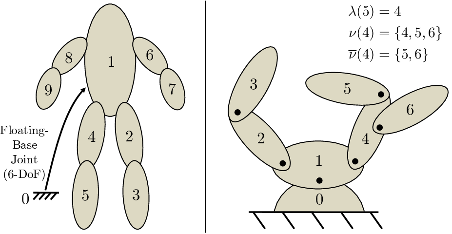
Refer to caption
Fig. 1: Convention examples with floating- and fixed-base systems.

Dynamics: The spatial equation of motion [12] is given for body kk as 𝒇k=𝑰​𝒂kk+𝒗k×∗𝑰​𝒗kk\boldsymbol{f}_{k}=\boldsymbol{I}{}_{k}\boldsymbol{a}_{k}+\boldsymbol{v}_{k}\times^{*}\boldsymbol{I}{}_{k}\boldsymbol{v}_{k}, where 𝒇k\boldsymbol{f}_{k} is the net spatial force on body kk, 𝑰k\boldsymbol{I}{}_{k} is its spatial inertia [12], and 𝒂k\boldsymbol{a}_{k} is its spatial acceleration. The development in Ref. [14] presents two additional spatial motion quantities 𝚿˙\dot{\boldsymbol{\Psi}}, 𝚿¨\ddot{\boldsymbol{\Psi}} (Eq. 5) essential to the derivation in this paper. The quantities 𝚿˙j\dot{\boldsymbol{\Psi}}_{j} and 𝚿¨j\ddot{\boldsymbol{\Psi}}_{j} represent the time-derivative of 𝑺j\boldsymbol{S}_{j}, and 𝚿˙j\dot{\boldsymbol{\Psi}}_{j}, respectively, due to joint jj’s predecessor λ⁡(j)\lambda(j) moving.

𝚿˙j=𝒗λ⁡(j)×𝑺j𝚿¨j=𝒂λ⁡(j)×𝑺j+𝒗λ⁡(j)×𝚿˙j\displaystyle\begin{split}\dot{\boldsymbol{\Psi}}_{j}=&\boldsymbol{v}_{\lambda(j)}\times\boldsymbol{S}_{j}\\ \ddot{\boldsymbol{\Psi}}_{j}=&\boldsymbol{a}_{\lambda(j)}\times\boldsymbol{S}_{j}+\boldsymbol{v}_{\lambda(j)}\times\dot{\boldsymbol{\Psi}}_{j}\end{split} (5)

The analytical expressions for the FO partial derivatives of ID w.r.t 𝒒\boldsymbol{q} and 𝒒˙\dot{\boldsymbol{q}} [14] are given below, with other similar formulations in [15, 16]. Here 𝝉i\boldsymbol{\tau}_{i} represents the joint torques/forces for joint ii from Eq. 1. The quantity 𝒇iC=∑k⪰i𝒇k\boldsymbol{f}{}_{i}^{C}=\sum_{k\succeq i}\boldsymbol{f}_{k} is the composite spatial force transmitted across joint ii, and 𝑰iC\boldsymbol{I}{}_{i}^{C} is the composite rigid-body inertia of the sub-tree rooted at body ii, given as 𝑰iC=∑k⪰i𝑰k\boldsymbol{I}{}{}_{i}^{C}=\sum_{k\succeq i}\boldsymbol{I}{}_{k}. The quantity 𝑩k\boldsymbol{B}{}_{k} is a body-level Coriolis matrix [14, 22],

𝑩=k12[(𝒗k×∗)𝑰−k𝑰(𝒗k×)k+(𝑰𝒗kk)ׯ]∗\boldsymbol{B}{}_{k}=\mathchoice{\scalebox{.75}{$\displaystyle\frac{1}{2}$}}{\scalebox{.75}{$\textstyle\frac{1}{2}$}}{\scalebox{.75}{$\scriptstyle\frac{1}{2}$}}{\scalebox{.75}{$\scriptscriptstyle\frac{1}{2}$}}[(\boldsymbol{v}_{k}\times^{*})\boldsymbol{I}{}_{k}-\boldsymbol{I}{}_{k}(\boldsymbol{v}_{k}\times)+(\boldsymbol{I}{}_{k}\boldsymbol{v}_{k})\,\overline{\!\times\!}{}^{\,*}] (6)

while 𝑩iC\boldsymbol{B}{}_{i}^{C} is its composite given by 𝑩iC=∑k⪰i𝑩k\boldsymbol{B}{}{}_{i}^{C}=\sum_{k\succeq i}\boldsymbol{B}{}_{k}. The next sections extend Eqs. 7-8 for SO derivatives of ID.

∂𝝉i∂𝒒j\displaystyle\frac{\partial{\boldsymbol{\tau}_{i}}}{\partial\boldsymbol{q}_{j}} =\displaystyle= 𝑺i⊤[2𝑩]Ci𝚿˙+j𝑺i⊤𝑰𝚿¨Ci,j(j⪯i)\displaystyle{\boldsymbol{S}_{i}^{\top}\big[2\boldsymbol{B}{}_{i}^{C}\big]\dot{\boldsymbol{\Psi}}{}_{j}+\boldsymbol{S}_{i}^{\top}\boldsymbol{I}{}_{i}^{C}\ddot{\boldsymbol{\Psi}}{}_{j}},(j\preceq i) (7a)
∂𝝉j∂𝒒i\displaystyle\frac{\partial{\boldsymbol{\tau}_{j}}}{\partial{\boldsymbol{q}_{i}}} =\displaystyle= 𝑺j⊤[2𝑩𝚿˙iCi+𝑰𝚿¨iCi+(𝒇iC)ׯ𝑺i∗],(j≺i)\displaystyle{\boldsymbol{S}_{j}^{\top}[2\boldsymbol{B}{}_{i}^{C}\dot{\boldsymbol{\Psi}}_{i}+\boldsymbol{I}{}_{i}^{C}\ddot{\boldsymbol{\Psi}}_{i}+(\boldsymbol{f}_{i}^{C})\,\overline{\!\times\!}{}^{\,*}\boldsymbol{S}_{i}],(j\prec i)}~~ (7b)
∂𝝉i∂𝒒˙j\displaystyle\frac{\partial{\boldsymbol{\tau}_{i}}}{\partial{\dot{\boldsymbol{q}}_{j}}} =\displaystyle= 𝑺i⊤[2𝑩𝑺jCi+𝑰(𝚿˙j+𝑺˙j)Ci],(j⪯i)\displaystyle{\boldsymbol{S}_{i}^{\top}\Big[2\boldsymbol{B}{}_{i}^{C}\boldsymbol{S}_{j}+\boldsymbol{I}{}_{i}^{C}(\dot{\boldsymbol{\Psi}}_{j}+\,\dot{\!\boldsymbol{S}}_{j})\Big],(j\preceq i)} (8a)
∂𝝉j∂𝒒˙i\displaystyle\frac{\partial{\boldsymbol{\tau}_{j}}}{\partial{\dot{\boldsymbol{q}}_{i}}} =\displaystyle= 𝑺j⊤[2𝑩𝑺iCi+𝑰(𝚿˙i+𝑺˙i)Ci],(j≺i)\displaystyle{\boldsymbol{S}_{j}^{\top}\Big[2\boldsymbol{B}{}_{i}^{C}\boldsymbol{S}_{i}+\boldsymbol{I}{}_{i}^{C}(\dot{\boldsymbol{\Psi}}_{i}+\,\dot{\!\boldsymbol{S}}_{i})\Big],(j\prec i)}~~~~~~~~\, (8b)

III Extending SVA For Tensorial Use

The motion space M6M^{6} [12] is extended to a space of spatial-motion matrices M6×nM^{6\times n}, where each column of such a matrix is a usual spatial motion vector. For any 𝑼∈M6×n\boldsymbol{U}\in M^{6\times n} a new spatial cross-product operator ×~{\tilde{\smash[t]{\times}}} is considered and defined by applying the usual spatial cross-product operator (×\times) to each column of 𝑼\boldsymbol{U}. The result is a third-order tensor (Fig. 2) in ℝ6×6×n\mathbb{R}^{6\times 6\times n} where each 6×66\times 6 matrix in the 1-2 dimension is the original spatial cross-product operator on a column of 𝑼\boldsymbol{U}.

Given two spatial motion matrices, 𝑼∈M6×nu\boldsymbol{U}\in M^{6\times n_{u}} and 𝑽∈M6×nv\boldsymbol{V}\in M^{6\times n_{v}} , we can now define a cross-product operation between them as (𝑼​×~)​𝑽∈M6×nv×nu(\boldsymbol{U}{\tilde{\smash[t]{\times}}})\boldsymbol{V}\in M^{6\times n_{v}\times n_{u}} via a tensor-matrix product. Such an operation, denoted as 𝒵=𝒜​𝑩\mathcal{Z}=\mathcal{A}\boldsymbol{B}{} is defined as:

𝒵i,j,k=∑ℓ𝒜i,ℓ,k​Bℓ,j\mathcal{Z}_{i,j,k}=\sum_{\ell}\mathcal{A}_{i,\ell,k}\\ B_{\ell,j} (9)

for any tensor 𝒜\mathcal{A} and suitably sized matrix 𝑩\boldsymbol{B}{}. Thus, the kk-th page, jj-th column of 𝑼​×~​𝑽\boldsymbol{U}{\tilde{\smash[t]{\times}}}\boldsymbol{V} gives the cross product of the kk-th column of 𝑼\boldsymbol{U} with the jj-th column of 𝑽\boldsymbol{V}.

In a similar manner, consider a spatial force matrix 𝑭∈F6×nf\boldsymbol{F}\in F^{6\times n_{f}}. Defining (𝑽×~)∗(\boldsymbol{V}{\tilde{\smash[t]{\times}}}{}^{*}) in an analogous manner to in Fig. 2 allows taking a cross-product-like operation 𝑽×~∗𝑭\boldsymbol{V}{\tilde{\smash[t]{\times}}}{}^{*}\boldsymbol{F}. Again, analogously, we consider a third operator (𝑭ׯ~)∗(\boldsymbol{F}\mathchoice{\scalebox{.87}{$\displaystyle\,\tilde{\bar{\smash[t]{\!\times\!}}{}}$}}{\scalebox{.87}{$\textstyle\,\tilde{\bar{\smash[t]{\!\times\!}}{}}$}}{\scalebox{.87}{$\scriptstyle\,\tilde{\bar{\smash[t]{\!\times\!}}{}}$}}{\scalebox{.87}{$\scriptscriptstyle\,\tilde{\bar{\smash[t]{\!\times\!}}{}}$}}{}^{\,*}) that provides 𝑽×~∗𝑭=𝑭ׯ~∗𝑽\boldsymbol{V}{\tilde{\smash[t]{\times}}}{}^{*}\boldsymbol{F}=\boldsymbol{F}\mathchoice{\scalebox{.87}{$\displaystyle\,\tilde{\bar{\smash[t]{\!\times\!}}{}}$}}{\scalebox{.87}{$\textstyle\,\tilde{\bar{\smash[t]{\!\times\!}}{}}$}}{\scalebox{.87}{$\scriptstyle\,\tilde{\bar{\smash[t]{\!\times\!}}{}}$}}{\scalebox{.87}{$\scriptscriptstyle\,\tilde{\bar{\smash[t]{\!\times\!}}{}}$}}{}^{\,*}\boldsymbol{V}. In each case, the tilde indicates the spatial-matrix extension of the usual spatial-vector cross products.

For later use, the product of a matrix 𝑩∈ℝn1×n2\boldsymbol{B}{}\in\mathbb{R}^{n_{1}\times n_{2}}, and a tensor 𝒜∈ℝn2×n3×n4\mathcal{A}\in\mathbb{R}^{n_{2}\times n_{3}\times n_{4}}, likewise results in another tensor, denoted as 𝒴=𝑩​𝒜\mathcal{Y}=\boldsymbol{B}{}\mathcal{A}, and defined as:

𝒴i,j,k=∑ℓ𝑩​𝒜ℓ,j,ki,ℓ\mathcal{Y}_{i,j,k}=\sum_{\ell}\boldsymbol{B}{}_{i,\ell}\mathcal{A}_{\ell,j,k} (10)
Refer to caption
Fig. 2: ×~{\tilde{\smash[t]{\times}}} operates on each column of a 𝑼∈M6×n\boldsymbol{U}\in M^{6\times n} spatial matrix to create a third-order tensor. Each rectangular box is a 2D matrix

Two types of tensor rotations are defined for this paper:

  1. 1.

    𝒜⊤~\mathcal{A}^{\widetilde{\top}}: Transpose along the 1-2 dimension. This operation can also be understood as the usual matrix transpose of each matrix (e.g., in Fig. 2) moving along pages of the tensor. If 𝒜⊤~=ℬ\mathcal{A}^{\widetilde{\top}}=\mathcal{B}, then 𝒜i,j,k=ℬj,i,k\mathcal{A}_{i,j,k}=\mathcal{B}_{j,i,k}.

  2. 2.

    𝒜R~\mathcal{A}^{\widetilde{\mathrm{R}}}: Rotation of elements along the 2-3 dimension. If 𝒜R~=ℬ\mathcal{A}^{\widetilde{\mathrm{R}}}=\mathcal{B}, then 𝒜i,j,k=ℬi,k,j\mathcal{A}_{i,j,k}=\mathcal{B}_{i,k,j}.

Another rotation (R~,⊤~{}^{\widetilde{\mathrm{R}},\widetilde{\!\top\!}}) is a combination of (R~)(^{\widetilde{\mathrm{R}}}) followed by (⊤~)(^{\widetilde{\top}}). For example, if 𝒜R~,⊤~=ℬ\mathcal{A}^{\widetilde{\mathrm{R}},\widetilde{\!\top\!}}=\mathcal{B}, then 𝒜i,j,k=ℬk,i,j\mathcal{A}_{i,j,k}=\mathcal{B}_{k,i,j}.

Properties of the operators are given in Table I. These properties naturally extend spatial vector properties [12], but with the added book-keeping required from using tensors. For example, the spatial force/vector cross-product operator ×∗{\times}^{*} satisfies 𝒗×∗=−𝒗×⊤\boldsymbol{v}{\times}^{*}=-\boldsymbol{v}\times^{\top}. Property M1 provides the matrix analogy for the spatial matrix operator ×~∗{\tilde{\smash[t]{\times}}}{}^{*}.

M1) 𝑼×~=∗−(𝑼×~)⊤~\boldsymbol{U}{\tilde{\smash[t]{\times}}}{}^{*}=-(\boldsymbol{U}{\tilde{\smash[t]{\times}}})^{\widetilde{\top}} M2) −𝑽⊤(𝑼×~)∗=(𝑼×~𝑽)⊤~-\boldsymbol{V}^{\top}(\boldsymbol{U}{\tilde{\smash[t]{\times}}}{}^{*})=(\boldsymbol{U}{\tilde{\smash[t]{\times}}}\boldsymbol{V})^{\widetilde{\top}} M3) −𝑽⊤(𝑼×~)∗𝑭=(𝑼×~𝑽)⊤~𝑭-\boldsymbol{V}^{\top}(\boldsymbol{U}{\tilde{\smash[t]{\times}}}{}^{*})\boldsymbol{F}=(\boldsymbol{U}{\tilde{\smash[t]{\times}}}\boldsymbol{V})^{\widetilde{\top}}\boldsymbol{F} M4) (𝑼×~𝒗)=−𝒗×𝑼(\boldsymbol{U}{\tilde{\smash[t]{\times}}}\boldsymbol{v})=-\boldsymbol{v}\times\boldsymbol{U} M5) 𝑼×~𝑭∗=(𝑭ׯ~𝑼∗)R~\boldsymbol{U}{\tilde{\smash[t]{\times}}}{}^{*}\boldsymbol{F}=(\boldsymbol{F}\mathchoice{\scalebox{.87}{$\displaystyle\,\tilde{\bar{\smash[t]{\!\times\!}}{}}$}}{\scalebox{.87}{$\textstyle\,\tilde{\bar{\smash[t]{\!\times\!}}{}}$}}{\scalebox{.87}{$\scriptstyle\,\tilde{\bar{\smash[t]{\!\times\!}}{}}$}}{\scalebox{.87}{$\scriptscriptstyle\,\tilde{\bar{\smash[t]{\!\times\!}}{}}$}}{}^{\,*}\boldsymbol{U})^{\widetilde{\mathrm{R}}} M6) 𝑭ׯ~𝑼∗=(𝑼×~𝑭∗)R~\boldsymbol{F}\mathchoice{\scalebox{.87}{$\displaystyle\,\tilde{\bar{\smash[t]{\!\times\!}}{}}$}}{\scalebox{.87}{$\textstyle\,\tilde{\bar{\smash[t]{\!\times\!}}{}}$}}{\scalebox{.87}{$\scriptstyle\,\tilde{\bar{\smash[t]{\!\times\!}}{}}$}}{\scalebox{.87}{$\scriptscriptstyle\,\tilde{\bar{\smash[t]{\!\times\!}}{}}$}}{}^{\,*}\boldsymbol{U}=(\boldsymbol{U}{\tilde{\smash[t]{\times}}}{}^{*}\boldsymbol{F})^{\widetilde{\mathrm{R}}} M7) (λ​𝑼)​×~=λ⁡(𝑼​×~)(\lambda\boldsymbol{U}){\tilde{\smash[t]{\times}}}=\lambda(\boldsymbol{U}{\tilde{\smash[t]{\times}}}) M8) 𝑼​×~​𝑽=−(𝑽​×~​𝑼)R~\boldsymbol{U}{\tilde{\smash[t]{\times}}}\boldsymbol{V}=-(\boldsymbol{V}{\tilde{\smash[t]{\times}}}\boldsymbol{U})^{\widetilde{\mathrm{R}}} M9) (𝒗×𝑼)×~=𝒗×𝑼×~−𝑼×~𝒗×(\boldsymbol{v}\times\boldsymbol{U}){\tilde{\smash[t]{\times}}}=\boldsymbol{v}\times\boldsymbol{U}{\tilde{\smash[t]{\times}}}-\boldsymbol{U}{\tilde{\smash[t]{\times}}}\boldsymbol{v}\times M10) (𝒗×𝑼)×~=∗𝒗×∗𝑼×~−∗𝑼×~𝒗∗×∗(\boldsymbol{v}\times\boldsymbol{U}){\tilde{\smash[t]{\times}}}{}^{*}=\boldsymbol{v}\times^{*}\boldsymbol{U}{\tilde{\smash[t]{\times}}}{}^{*}-\boldsymbol{U}{\tilde{\smash[t]{\times}}}{}^{*}\boldsymbol{v}\times^{*} M11) (𝑼×~𝒗∗)ׯ~=∗𝑼×~𝒗∗ׯ−∗𝒗ׯ𝑼∗×~(\boldsymbol{U}{\tilde{\smash[t]{\times}}}{}^{*}\boldsymbol{v})\mathchoice{\scalebox{.87}{$\displaystyle\,\tilde{\bar{\smash[t]{\!\times\!}}{}}$}}{\scalebox{.87}{$\textstyle\,\tilde{\bar{\smash[t]{\!\times\!}}{}}$}}{\scalebox{.87}{$\scriptstyle\,\tilde{\bar{\smash[t]{\!\times\!}}{}}$}}{\scalebox{.87}{$\scriptscriptstyle\,\tilde{\bar{\smash[t]{\!\times\!}}{}}$}}{}^{\,*}=\boldsymbol{U}{\tilde{\smash[t]{\times}}}{}^{*}\boldsymbol{v}\,\overline{\!\times\!}{}^{\,*}-\boldsymbol{v}\,\overline{\!\times\!}{}^{\,*}\boldsymbol{U}{\tilde{\smash[t]{\times}}} M12) (𝑼×~𝑭∗)⊤~=−𝑭⊤(𝑼×~)(\boldsymbol{U}{\tilde{\smash[t]{\times}}}{}^{*}\boldsymbol{F})^{\widetilde{\top}}=-\boldsymbol{F}^{\top}(\boldsymbol{U}{\tilde{\smash[t]{\times}}}) M13) 𝑽⊤(𝑼×~𝑭∗)=(𝑽×~𝑼)R~,⊤~𝑭=(𝑭⊤(𝑽×~𝑼)R~)⊤~\boldsymbol{V}^{\top}(\boldsymbol{U}{\tilde{\smash[t]{\times}}}{}^{*}\boldsymbol{F})=(\boldsymbol{V}{\tilde{\smash[t]{\times}}}\boldsymbol{U})^{\widetilde{\mathrm{R}},\widetilde{\!\top\!}}\boldsymbol{F}=(\boldsymbol{F}^{\top}(\boldsymbol{V}{\tilde{\smash[t]{\times}}}\boldsymbol{U})^{\widetilde{\mathrm{R}}})^{\widetilde{\top}} M14) 𝒗×∗𝑭=𝑭ׯ~∗𝒗\boldsymbol{v}\times^{*}\boldsymbol{F}=\boldsymbol{F}\mathchoice{\scalebox{.87}{$\displaystyle\,\tilde{\bar{\smash[t]{\!\times\!}}{}}$}}{\scalebox{.87}{$\textstyle\,\tilde{\bar{\smash[t]{\!\times\!}}{}}$}}{\scalebox{.87}{$\scriptstyle\,\tilde{\bar{\smash[t]{\!\times\!}}{}}$}}{\scalebox{.87}{$\scriptscriptstyle\,\tilde{\bar{\smash[t]{\!\times\!}}{}}$}}{}^{\,*}\boldsymbol{v} M15) 𝒇ׯ∗𝑼=𝑼×~∗𝒇\boldsymbol{f}\,\overline{\!\times\!}{}^{\,*}\boldsymbol{U}=\boldsymbol{U}{\tilde{\smash[t]{\times}}}{}^{*}\boldsymbol{f} M16) 𝑽⊤(𝑼×~𝑭∗)R~=[(𝑽×~𝑼)R~,⊤~𝑭]R~\boldsymbol{V}^{\top}(\boldsymbol{U}{\tilde{\smash[t]{\times}}}{}^{*}\boldsymbol{F})^{\widetilde{\mathrm{R}}}=\big[(\boldsymbol{V}{\tilde{\smash[t]{\times}}}\boldsymbol{U})^{\widetilde{\mathrm{R}},\widetilde{\!\top\!}}\boldsymbol{F}\big]^{\widetilde{\mathrm{R}}} M17) 𝑽⊤(𝑼×~𝑭∗)R~=−[𝑼⊤(𝑽×~𝑭∗)R~]⊤~\boldsymbol{V}^{\top}(\boldsymbol{U}{\tilde{\smash[t]{\times}}}{}^{*}\boldsymbol{F})^{\widetilde{\mathrm{R}}}=-[\boldsymbol{U}^{\top}(\boldsymbol{V}{\tilde{\smash[t]{\times}}}{}^{*}\boldsymbol{F})^{\widetilde{\mathrm{R}}}]^{\widetilde{\top}} M18) 𝑽⊤(𝑼×~𝑭∗)R~=[𝑽⊤(𝑼×~𝑭∗)]R~\boldsymbol{V}^{\top}(\boldsymbol{U}{\tilde{\smash[t]{\times}}}{}^{*}\boldsymbol{F})^{\widetilde{\mathrm{R}}}=[\boldsymbol{V}^{\top}(\boldsymbol{U}{\tilde{\smash[t]{\times}}}{}^{*}\boldsymbol{F})]^{\widetilde{\mathrm{R}}} M19) (𝑩𝒴)⊤~=𝒴⊤~𝑩⊤(\boldsymbol{B}{}\mathcal{Y})^{\widetilde{\top}}=\mathcal{Y}^{\widetilde{\top}}\boldsymbol{B}{}^{\top}

TABLE I: Spatial Matrix Algebra Identities: 𝒗∈M6\boldsymbol{v}\in M^{6},𝒇∈F6\boldsymbol{f}\in F^{6}, 𝑼∈M6×n\boldsymbol{U}\in M^{6\times n}, 𝑭∈F6×m\boldsymbol{F}\in F^{6\times m}, 𝑽∈M6×l\boldsymbol{V}\in M^{6\times l}, 𝑩∈ℝn1×n2\boldsymbol{B}{}\in\mathbb{R}^{n_{1}\times n_{2}}, 𝒴∈ℝn2×n3×n4\mathcal{Y}\in\mathbb{R}^{n_{2}\times n_{3}\times n_{4}}.

IV Second-Order Derivatives of ID

IV-A Preliminaries

The SO partial derivative of joint torque/force is also referred to as a dynamics Hessian tensor. Blocks of this rank 3 tensor are written in a form ∂2𝝉i∂𝒖j​∂𝒖k\frac{\partial^{2}\boldsymbol{\tau}_{i}}{\partial\boldsymbol{u}_{j}\partial\boldsymbol{u}_{k}}, which signifies taking partial derivative of 𝝉i\boldsymbol{\tau}_{i} w.r.t 𝒖j\boldsymbol{u}_{j}, followed by 𝒖k\boldsymbol{u}_{k}. The variables 𝒖j\boldsymbol{u}_{j} and 𝒖k\boldsymbol{u}_{k} can either be the joint configuration (𝒒j\boldsymbol{q}_{j}, 𝒒k\boldsymbol{q}_{k}), joint velocity (𝒒˙j\dot{\boldsymbol{q}}_{j}, 𝒒˙k\dot{\boldsymbol{q}}_{k}), or joint acceleration (𝒒¨j\ddot{\boldsymbol{q}}_{j}, 𝒒¨k\ddot{\boldsymbol{q}}_{k}). Many of these second-order partials are zero, limiting the cases to be considered. From Eq. 1, the first-order partial derivative of 𝝉\boldsymbol{\tau}{} w.r.t 𝒒¨\ddot{\boldsymbol{q}} is ∂𝝉/∂𝒒¨=𝑴⁡(𝒒){\partial\boldsymbol{\tau}}/{\partial\ddot{\boldsymbol{q}}}=\boldsymbol{M}(\boldsymbol{q}). Taking subsequent partial derivatives results in ∂2𝝉/∂𝒒¨​∂𝒒¨=0{\partial^{2}\boldsymbol{\tau}}/{\partial\ddot{\boldsymbol{q}}\partial\ddot{\boldsymbol{q}}}=0 and ∂2𝝉/∂𝒒¨​∂𝒒˙=0{\partial^{2}\boldsymbol{\tau}}/{\partial\ddot{\boldsymbol{q}}\partial\dot{\boldsymbol{q}}}=0. However, the cross-derivative w.r.t 𝒒¨\ddot{\boldsymbol{q}} and 𝒒\boldsymbol{q} is non-trivial and equals ∂𝑴⁡(𝒒)/∂𝒒{\partial\boldsymbol{M}(\boldsymbol{q})}/{\partial\boldsymbol{q}}. Garofalo et al. [23] present formulas for the partial derivative of 𝑴⁡(𝒒)\boldsymbol{M}(\boldsymbol{q}) w.r.t 𝒒\boldsymbol{q} for multi-DoF Lie group joints. In this work, we re-derive that result using newly developed spatial matrix operators and contribute new analytical SO partial derivatives of ID w.r.t 𝒒\boldsymbol{q} and 𝒒˙\dot{\boldsymbol{q}}.

For single-DoF joints, each block of the Hessian tensor ∂2𝝉i∂𝒖j​∂𝒖k\frac{\partial^{2}\boldsymbol{\tau}_{i}}{\partial\boldsymbol{u}_{j}\partial\boldsymbol{u}_{k}} is a scalar representing a conventional SO derivative w.r.t joint angles, rates, or accelerations. In this case, the order of 𝒖j\boldsymbol{u}_{j} and 𝒖k\boldsymbol{u}_{k} doesn’t matter. This operation becomes more nuanced when considering derivatives w.r.t configuration for a multi-DoF joint, wherein we define the operator ∂∂𝒒k\frac{\partial}{\partial\boldsymbol{q}_{k}} to represent a collection of Lie derivatives, as in [14]. For example, ∂𝝉i∂𝒒k\frac{\partial\boldsymbol{\tau}_{i}}{\partial\boldsymbol{q}_{k}} is defined as the ni×nkn_{i}\times n_{k} matrix where each column gives the derivative of 𝝉i∈ℝni\boldsymbol{\tau}_{i}\in\mathbb{R}^{n_{i}} w.r.t changes in configuration along one of the nkn_{k} free modes of joint kk (see [14] for detail). When the Lie derivatives along the free modes of a joint do not commute, ∂2𝝉i∂𝒒k​∂𝒒k\frac{\partial^{2}\boldsymbol{\tau}_{i}}{\partial\boldsymbol{q}_{k}\partial\boldsymbol{q}_{k}} can lack the usual symmetry properties. Such a case occurs, for example, with a spherical joint, since rotations do not commute. To obtain the partial derivatives of spatial quantities embedded in Eq. 7-8, some identities (App. A) are derived. These are an extension to ones defined in Ref. [14], but use the newly developed spatial matrix operators from Sec. III.

For example, identity K1 (App. A) is an extension of identity J1 in Ref. [14]. The identity J1 (Eq. 11) gives the directional derivative of the joint motion sub-space matrix 𝑺i\boldsymbol{S}_{i} w.r.t the pt​hp^{th} DoF of a previous joint jj in the connectivity tree:

∂𝑺i∂𝒒j,p=𝒔j,p×𝑺i​(j⪯i)\frac{\partial\boldsymbol{S}_{i}}{\partial\boldsymbol{q}_{j,p}}=\boldsymbol{s}_{j,p}\times\boldsymbol{S}_{i}~~~(j\preceq i) (11)

where 𝒔j,p\boldsymbol{s}_{j,p} is the pp-th column of 𝑺j\boldsymbol{S}_{j}. On the other hand, K1 uses the ×~{\tilde{\smash[t]{\times}}} operator to extend it to the partial derivative of 𝑺i\boldsymbol{S}_{i} w.r.t the full joint configuration 𝒒j\boldsymbol{q}_{j} to give the tensor ∂𝑺i∂𝒒j\frac{\partial\boldsymbol{S}_{i}}{\partial\boldsymbol{q}_{j}} as:

∂𝑺i∂𝒒j=𝑺j​×~​𝑺i​(j⪯i)\frac{\partial\boldsymbol{S}_{i}}{\partial\boldsymbol{q}_{j}}=\boldsymbol{S}_{j}{\tilde{\smash[t]{\times}}}\boldsymbol{S}_{i}~~~(j\preceq i) (12)

The identities K4 and K9 describe the partial derivatives of 𝚿˙i\dot{\boldsymbol{\Psi}}_{i} and 𝚿¨i\ddot{\boldsymbol{\Psi}}_{i} present in Eq. 7-8. Identities K6, K10, and K12 give the partial derivatives of the composite Inertia (𝑰iC\boldsymbol{I}{}_{i}^{C}), body-level Coriolis matrix (𝑩iC\boldsymbol{B}{}_{i}^{C}), and net composite spatial force on a body (𝒇iC\boldsymbol{f}_{i}^{C}). Individual partial derivatives of these quantities allow us to use the plug-and-play approach to simplify the algebra needed for SO partial derivatives of ID.

To calculate the SO partial derivatives, we take subsequent partial derivatives of the terms ∂𝝉i∂𝒒j\frac{\partial\boldsymbol{\tau}_{i}}{\partial\boldsymbol{q}_{j}}, ∂𝝉j∂𝒒i\frac{\partial\boldsymbol{\tau}_{j}}{\partial\boldsymbol{q}_{i}},∂𝝉i∂𝒒˙j\frac{\partial\boldsymbol{\tau}_{i}}{\partial\dot{\boldsymbol{q}}_{j}}, and ∂𝝉j∂𝒒˙i\frac{\partial\boldsymbol{\tau}_{j}}{\partial\dot{\boldsymbol{q}}_{i}} w.r.t joint configuration (𝒒\boldsymbol{q}), and joint velocity (𝒒˙\dot{\boldsymbol{q}}) for joint kk. We consider three cases, by changing the order of index kk as:

Case A:k⪯j⪯iCase B:j≺k⪯iCase C:j⪯i≺k\textbf{Case~A:}~k\preceq j\preceq i~~~\textbf{Case~B:}~j\prec k\preceq i~~~\textbf{Case~C:}~j\preceq i\prec k

The sections below outline the approach for calculating the SO partial derivatives. Only some cases are shown to illustrate the main idea, with a detailed summary of all the cases in App. B, and full step-by-step derivations in Ref. [19].

IV-B Second-order partial derivatives w.r.t 𝐪\boldsymbol{q}

For SO partials of ID w.r.t 𝒒\boldsymbol{q}, we take the partial derivatives of Eq. 7a, and 7b w.r.t 𝒒k\boldsymbol{q}_{k} for cases A, B, and C mentioned above. Although, the symmetric blocks in the Hessian allow us to re-use three of those six cases. For any of the cases, the partial derivatives of Eq. 7a and 7b can be taken, as long as the accompanying conditions on the equations are met. For example, for Case B (j≺k⪯ij\prec k\preceq i), since j≺ij\prec i, only Eq. 7b can be used. A derivation for Case C (j⪯i≺kj\preceq i\prec k) is shown here as an example. We take the partial derivative of Eq. 7a w.r.t 𝒒k\boldsymbol{q}_{k}. Applying the product rule, and using the identities K4, K9, and K13 as:

∂2𝝉i∂𝒒j​∂𝒒k=2𝑺i⊤(∂𝑩iC∂𝒒k𝚿˙)j+𝑺i⊤(∂𝑰iC∂𝒒k𝚿¨)j\frac{\partial^{2}\boldsymbol{\tau}_{i}}{\partial\boldsymbol{q}_{j}\partial\boldsymbol{q}_{k}}=2\boldsymbol{S}_{i}^{\top}\left(\frac{\partial\boldsymbol{B}{}_{i}^{C}}{\partial\boldsymbol{q}_{k}}\dot{\boldsymbol{\Psi}}{}_{j}\right)+\boldsymbol{S}_{i}^{\top}\left(\frac{\partial\boldsymbol{I}{}_{i}^{C}}{\partial\boldsymbol{q}_{k}}\ddot{\boldsymbol{\Psi}}{}_{j}\right) (13)

The quantities ∂𝑩iC∂𝒒k\frac{\partial\boldsymbol{B}{}_{i}^{C}}{\partial\boldsymbol{q}_{k}} and ∂𝑰iC∂𝒒k\frac{\partial\boldsymbol{I}{}_{i}^{C}}{\partial\boldsymbol{q}_{k}} are third-order tensors where the partial derivatives of matrices 𝑩iC\boldsymbol{B}{}_{i}^{C} and 𝑰iC\boldsymbol{I}{}_{i}^{C} w.r.t each DoF of joint kk are stacked as matrices along the pages of the tensor. Using the identities K6 and K10 then gives:

∂2𝝉i∂𝒒j​∂𝒒k=2𝑺i⊤(ℬkC[𝚿˙k]+𝑺k×~𝑩∗−Ck𝑩(𝑺k×~)Ck)𝚿˙j\displaystyle\frac{\partial^{2}\boldsymbol{\tau}_{i}}{\partial\boldsymbol{q}_{j}\partial\boldsymbol{q}_{k}}=2\boldsymbol{S}_{i}^{\top}\Big(\mathcal{B}_{k}^{C}\big[\dot{\boldsymbol{\Psi}}_{k}\big]+\boldsymbol{S}_{k}{\tilde{\smash[t]{\times}}}{}^{*}\boldsymbol{B}{}_{k}^{C}-\boldsymbol{B}{}_{k}^{C}(\boldsymbol{S}_{k}{\tilde{\smash[t]{\times}}})\Big)\dot{\boldsymbol{\Psi}}_{j}
+𝑺i⊤(𝑺k×~𝑰∗−Ck𝑰(𝑺k×~)Ck)𝚿¨j\displaystyle~~~~~~~~~~~~~~~~~~~~~+\boldsymbol{S}_{i}^{\top}\Big(\boldsymbol{S}_{k}{\tilde{\smash[t]{\times}}}{}^{*}\boldsymbol{I}{}_{k}^{C}-\boldsymbol{I}{}_{k}^{C}(\boldsymbol{S}_{k}{\tilde{\smash[t]{\times}}})\Big)\ddot{\boldsymbol{\Psi}}_{j} (14)

where the tensor ℬkC​[𝚿˙k]\mathcal{B}_{k}^{C}\big[\dot{\boldsymbol{\Psi}}_{k}\big] is a composite calculated for the sub-tree as ℬkC​[𝚿˙k]=∑l⪰kℬl​[𝚿˙k]\mathcal{B}_{k}^{C}\big[\dot{\boldsymbol{\Psi}}_{k}\big]=\sum_{l\succeq k}\mathcal{B}_{l}[\dot{\boldsymbol{\Psi}}_{k}], with:

ℬl[𝚿˙k]=12[(𝚿˙k×~)∗𝑰−l𝑰(𝚿˙k×~)l+(𝑰𝚿˙kl)ׯ~]∗\mathcal{B}_{l}\big[\dot{\boldsymbol{\Psi}}_{k}\big]=\frac{1}{2}\big[\big(\dot{\boldsymbol{\Psi}}_{k}{\tilde{\smash[t]{\times}}}{}^{*}\big)\boldsymbol{I}{}_{l}-\boldsymbol{I}{}_{l}\big(\dot{\boldsymbol{\Psi}}_{k}{\tilde{\smash[t]{\times}}}\big)+\big(\boldsymbol{I}{}_{l}\dot{\boldsymbol{\Psi}}_{k}\big)\mathchoice{\scalebox{.87}{$\displaystyle\,\tilde{\bar{\smash[t]{\!\times\!}}{}}$}}{\scalebox{.87}{$\textstyle\,\tilde{\bar{\smash[t]{\!\times\!}}{}}$}}{\scalebox{.87}{$\scriptstyle\,\tilde{\bar{\smash[t]{\!\times\!}}{}}$}}{\scalebox{.87}{$\scriptscriptstyle\,\tilde{\bar{\smash[t]{\!\times\!}}{}}$}}{}^{\,*}\big] (15)

Eq. 15 is a tensor extension of the body-level Coriolis matrix (Eq. 6) with a spatial matrix argument. Expressions for other cases are in App. B with full derivation in Ref. [19, Sec. IV].

IV-C Cross Second Order Partial derivatives w.r.t 𝐪¨\ddot{\boldsymbol{q}} and 𝐪\boldsymbol{q}

As explained before, the cross-SO partial derivatives of ID w.r.t 𝒒¨\ddot{\boldsymbol{q}} and 𝒒\boldsymbol{q} results in ∂𝑴∂𝒒\frac{\partial\boldsymbol{M}}{\partial\boldsymbol{q}}. The lower-triangle of the mass matrix 𝑴⁡(𝒒)\boldsymbol{M}(\boldsymbol{q}) for the case j⪯ij\preceq i is given as [12]:

𝑴j​i=𝑺j⊤​𝑰​𝑺iiC\boldsymbol{M}_{ji}=\boldsymbol{S}_{j}^{\top}\boldsymbol{I}{}_{i}^{C}\boldsymbol{S}_{i} (16)

Since 𝑴⁡(𝒒)\boldsymbol{M}(\boldsymbol{q}) is symmetric [12], 𝑴i​j=𝑴j​i⊤\boldsymbol{M}_{ij}=\boldsymbol{M}_{ji}^{\top}. We apply the three cases A, B, and C discussed before. As an example, for Case B (j≺k⪯ij\prec k\preceq i), we take the partial derivative of 𝑴j​i\boldsymbol{M}_{ji} w.r.t 𝒒k\boldsymbol{q}_{k} and use the product rule, along with identity K13 as:

∂𝑴j​i∂𝒒k=𝑺j⊤​(∂𝑰iC∂𝒒k​𝑺i+𝑰​∂𝑺i∂𝒒kiC)\frac{\partial\boldsymbol{M}_{ji}}{\partial\boldsymbol{q}_{k}}=\boldsymbol{S}_{j}^{\top}\left(\frac{\partial\boldsymbol{I}{}_{i}^{C}}{\partial\boldsymbol{q}_{k}}\boldsymbol{S}_{i}+\boldsymbol{I}{}_{i}^{C}\frac{\partial\boldsymbol{S}_{i}}{\partial\boldsymbol{q}_{k}}\right) (17)

Using with identities K1 and K6, and canceling terms gives:

∂𝑴j​i∂𝒒k=𝑺j⊤(𝑺k×~𝑰∗)Ci𝑺i\frac{\partial\boldsymbol{M}_{ji}}{\partial\boldsymbol{q}_{k}}=\boldsymbol{S}_{j}^{\top}(\boldsymbol{S}_{k}{\tilde{\smash[t]{\times}}}{}^{*}\boldsymbol{I}{}_{i}^{C})\boldsymbol{S}_{i} (18)

Expressions for other cases are listed in App. B, with details of derivation at Ref. [19, Sec. VII]

IV-D Second-order partial derivatives involving 𝐪˙\dot{\boldsymbol{q}}

For SO partial derivatives w.r.t 𝒒˙\dot{\boldsymbol{q}}, we take the partial derivatives of Eq. 8a and 8b w.r.t 𝒒˙k\dot{\boldsymbol{q}}_{k}. A list of expressions is given in App. B, with full derivation in Ref. [19, Sec. V].

For cross-SO partial derivatives of ID, we take the partial derivative of Eqs. 8a-8b w.r.t 𝒒k\boldsymbol{q}_{k} to get ∂2𝝉∂𝒒˙​∂𝒒\frac{\partial^{2}\boldsymbol{\tau}}{\partial\dot{\boldsymbol{q}}\partial\boldsymbol{q}}. The three cases A,B, and C (Sec. IV-A) for Eq. 8a-8b result in six expressions, which are then also used for the symmetric term ∂2𝝉∂𝒒​∂𝒒˙\frac{\partial^{2}\boldsymbol{\tau}}{\partial\boldsymbol{q}\partial\dot{\boldsymbol{q}}} as:

∂2𝝉∂𝒒​∂𝒒˙=[∂2𝝉∂𝒒˙​∂𝒒]R~\frac{\partial^{2}\boldsymbol{\tau}}{\partial\boldsymbol{q}\partial\dot{\boldsymbol{q}}}=\left[\frac{\partial^{2}\boldsymbol{\tau}}{\partial\dot{\boldsymbol{q}}\partial\boldsymbol{q}}\right]{\!\vphantom{\Big)}}^{\widetilde{\mathrm{R}}} (19)

Here, we solve all the three cases A, B and C for both Eq. 8a and Eq. 8b. Pertaining to Case A (k⪯j⪯ik\preceq j\preceq i), since j⪯ij\preceq i, Eq. 8a can be safely used to get ∂2𝝉i∂𝒒˙j​∂𝒒k\frac{\partial^{2}\boldsymbol{\tau}_{i}}{\partial\dot{\boldsymbol{q}}_{j}\partial\boldsymbol{q}_{k}}. However, the j≠ij\neq i requirement on Eq. 8b constrains the condition in Case A to k⪯j≺ik\preceq j\prec i. Similarly, for Case C (j⪯i≺kj\preceq i\prec k), taking partial derivative of Eq. 8b results in a stricter case j≺i≺kj\prec i\prec k. Appendix B lists the six expressions with full derivation in Ref. [19, Sec. VI].

V Efficient Implementation and Algorithm

For efficient implementation of the algorithm, all the cases are converted to an index order of k⪯j⪯ik\preceq j\preceq i. This notation is explained with the help of following two examples.

Example 1: In Eq. 14, we first we switch the indices kk and jj, followed by jj and ii to get ∂2𝝉j∂𝒒k​∂𝒒i\frac{\partial^{2}\boldsymbol{\tau}_{j}}{\partial\boldsymbol{q}_{k}\partial\boldsymbol{q}_{i}} as

∂2𝝉j∂𝒒k​∂𝒒i=2𝑺j⊤(ℬiC[𝚿˙i]+𝑺i×~𝑩∗−Ci𝑩(𝑺i×~)Ci)𝚿˙k\displaystyle\frac{\partial^{2}\boldsymbol{\tau}_{j}}{\partial\boldsymbol{q}_{k}\partial\boldsymbol{q}_{i}}=2\boldsymbol{S}_{j}^{\top}\Big(\mathcal{B}_{i}^{C}\big[\dot{\boldsymbol{\Psi}}_{i}\big]+\boldsymbol{S}_{i}{\tilde{\smash[t]{\times}}}{}^{*}\boldsymbol{B}{}_{i}^{C}-\boldsymbol{B}{}_{i}^{C}(\boldsymbol{S}_{i}{\tilde{\smash[t]{\times}}})\Big)\dot{\boldsymbol{\Psi}}_{k}
+𝑺j⊤(𝑺i×~𝑰∗−Ci𝑰(𝑺i×~)Ci)𝚿¨k\displaystyle~~~~~~~~~~~~~~~+\boldsymbol{S}_{j}^{\top}\Big(\boldsymbol{S}_{i}{\tilde{\smash[t]{\times}}}{}^{*}\boldsymbol{I}{}_{i}^{C}-\boldsymbol{I}{}_{i}^{C}(\boldsymbol{S}_{i}{\tilde{\smash[t]{\times}}})\Big)\ddot{\boldsymbol{\Psi}}_{k} (20)

For the term ∂2𝝉j∂𝒒i​∂𝒒k\frac{\partial^{2}\boldsymbol{\tau}_{j}}{\partial\boldsymbol{q}_{i}\partial\boldsymbol{q}_{k}}, when k≠ik\neq i, the symmetry property of Hessian blocks can be exploited:

∂2𝝉j∂𝒒i​∂𝒒k=[∂2𝝉j∂𝒒k​∂𝒒i]R~,(k⪯j≺i)\frac{\partial^{2}\boldsymbol{\tau}_{j}}{\partial\boldsymbol{q}_{i}\partial\boldsymbol{q}_{k}}=\left[\frac{\partial^{2}\boldsymbol{\tau}_{j}}{\partial\boldsymbol{q}_{k}\partial\boldsymbol{q}_{i}}\right]{\!\vphantom{\Big)}}^{\widetilde{\mathrm{R}}},(k\preceq j\prec i) (21)

The 2-3 tensor rotation in Eq. 21 occurs due to symmetry along the 2nd and 3rd dimensions.

Example 2: In Eq. 18, switching indices kk and jj leads to the index order k≺j⪯ik\prec j\preceq i. Using property M5 leads to:

∂𝑴k​i∂𝒒j=𝑺k⊤((𝑰𝑺iCi)ׯ~𝑺j∗)R~\frac{\partial\boldsymbol{M}_{ki}}{\partial\boldsymbol{q}_{j}}=\boldsymbol{S}_{k}^{\top}((\boldsymbol{I}{}_{i}^{C}\boldsymbol{S}_{i})\mathchoice{\scalebox{.87}{$\displaystyle\,\tilde{\bar{\smash[t]{\!\times\!}}{}}$}}{\scalebox{.87}{$\textstyle\,\tilde{\bar{\smash[t]{\!\times\!}}{}}$}}{\scalebox{.87}{$\scriptstyle\,\tilde{\bar{\smash[t]{\!\times\!}}{}}$}}{\scalebox{.87}{$\scriptscriptstyle\,\tilde{\bar{\smash[t]{\!\times\!}}{}}$}}{}^{\,*}\boldsymbol{S}_{j})^{\widetilde{\mathrm{R}}} (22)

Symmetry of 𝑴⁡(𝒒)\boldsymbol{M}(\boldsymbol{q}) gives us ∂𝑴i​k∂𝒒j\frac{\partial\boldsymbol{M}_{ik}}{\partial\boldsymbol{q}_{j}} as:

∂𝑴i​k∂𝒒j=[∂𝑴k​i∂𝒒j]⊤~\small\frac{\partial\boldsymbol{M}_{ik}}{\partial\boldsymbol{q}_{j}}=\left[\frac{\partial\boldsymbol{M}_{ki}}{\partial\boldsymbol{q}_{j}}\right]^{\widetilde{\top}} (23)

In this case, since the symmetry is along the 1st and the 2nd dimension of ∂𝑴k​i∂𝒒j\frac{\partial\boldsymbol{M}_{ki}}{\partial\boldsymbol{q}_{j}}, the tensor 1-2 rotation takes place.

The expressions for SO partials of ID (App. B) are first reduced to matrix and vector form to avoid tensor operations. This refactoring is due, in part, to a lack of stable tensor support in the C++ Eigen library that is often used in robotics dynamics libraries. This reduction is achieved by considering the expressions for single DoF of joints ii, jj, and kk, one at a time. We explain this process with the help of two examples.

Example 1: Considering the case k≺j⪯ik\prec j\preceq i the expression

∂2𝝉i∂𝒒˙j​∂𝒒˙k=−[𝑺j⊤​(2​ℬiC​[𝑺i]​𝑺k)R~]⊤~\small\frac{\partial^{2}\boldsymbol{\tau}_{i}}{\partial\dot{\boldsymbol{q}}_{j}\partial\dot{\boldsymbol{q}}_{k}}=-\big[\boldsymbol{S}_{j}^{\top}(2\mathcal{B}_{i}^{C}[\boldsymbol{S}_{i}]\boldsymbol{S}_{k})^{\widetilde{\mathrm{R}}}\big]^{\widetilde{\top}}

is studied for the pt​hp^{th}, tt​ht^{th}, and rt​hr^{th} DoFs of the joints ii, jj and kk, respectively. The tensor term ℬiC​[𝑺i]\mathcal{B}_{i}^{C}[\boldsymbol{S}_{i}] (defined by Eq. 15) reduces to a matrix 𝑩[𝒔i,p]Ci\boldsymbol{B}{}_{i}^{C}[\boldsymbol{s}_{i,p}], where 𝒔i,p\boldsymbol{s}_{i,p} is pp-th column of 𝑺i\boldsymbol{S}_{i}. This term represents the value 𝑩iC\boldsymbol{B}{}_{i}^{C} would take if all bodies in the subtree at ii moved with velocity 𝒔i,p\boldsymbol{s}_{i,p}. The above reduction enables dropping the 3D tensor rotation (R~)(^{\widetilde{\mathrm{R}}}). The products of 𝑩[𝒔i,p]Ci\boldsymbol{B}{}_{i}^{C}[\boldsymbol{s}_{i,p}] with column vectors 𝒔j,t\boldsymbol{s}_{j,t} and 𝒔k,r\boldsymbol{s}_{k,r} then provides a scalar, resulting in dropping the rotation (⊤~)(^{\widetilde{\top}}) from above:

∂2𝝉i,p∂𝒒˙j,t​∂𝒒˙k,r=−2𝒔j,t⊤(𝑩[𝒔i,p]Ci𝒔k,r)\small\frac{\partial^{2}\boldsymbol{\tau}_{i,p}}{\partial\dot{\boldsymbol{q}}_{j,t}\partial\dot{\boldsymbol{q}}_{k,r}}=-2\boldsymbol{s}_{j,t}^{\top}\big(\boldsymbol{B}{}_{i}^{C}[\boldsymbol{s}_{i,p}]\boldsymbol{s}_{k,r}\big) (24)

Example 2: The term ∂2𝝉i∂𝒒˙k​∂𝒒˙j=[∂2𝝉i∂𝒒˙j​∂𝒒˙k]R~\frac{\partial^{2}\boldsymbol{\tau}_{i}}{\partial\dot{\boldsymbol{q}}_{k}\partial\dot{\boldsymbol{q}}_{j}}=\left[\frac{\partial^{2}\boldsymbol{\tau}_{i}}{\partial\dot{\boldsymbol{q}}_{j}\partial\dot{\boldsymbol{q}}_{k}}\right]^{\widetilde{\mathrm{R}}} is evaluated for the pt​hp^{th}, tt​ht^{th}, and rt​hr^{th} DoFs of the joints ii, jj and kk, respectively. In this case, the 2-3 tensor rotation (R~{}^{\widetilde{\mathrm{R}}}) drops out, since the resulting expression is a scalar.

∂2𝝉i,p∂𝒒˙k,r​∂𝒒˙j,t=∂2𝝉i,p∂𝒒˙j,t​∂𝒒˙k,r\small\frac{\partial^{2}\boldsymbol{\tau}_{i,p}}{\partial\dot{\boldsymbol{q}}_{k,r}\partial\dot{\boldsymbol{q}}_{j,t}}=\frac{\partial^{2}\boldsymbol{\tau}_{i,p}}{\partial\dot{\boldsymbol{q}}_{j,t}\partial\dot{\boldsymbol{q}}_{k,r}} (25)

Algorithm 1 (IDSVA SO) is detailed in App. B and returns all the SO partials from Sec. IV. It is implemented with all kinematic and dynamic quantities represented in the ground frame. The forward pass in Alg. 1 (Lines 2-11) solves for kinematic and dynamic quantities like 𝒂i\boldsymbol{a}_{i}, 𝑩iC\boldsymbol{B}{}_{i}^{C}, 𝒇iC\boldsymbol{f}{}_{i}^{C}, 𝚿˙i\dot{\boldsymbol{\Psi}}_{i}, and 𝚿¨i\ddot{\boldsymbol{\Psi}}_{i} for the entire tree. The quantity 12\frac{1}{2} is skipped from the definition of 𝑩iC\boldsymbol{B}{}_{i}^{C} to make algebra simpler, and necessary adjustments are made in the algorithm. The backward pass then cycles from leaves to root of the tree and consists of three main nested loops, each one for bodies ii, jj, and kk. These three nested loops also consist of a nested loop for each DoF of joint ii, jj, and kk. The indices pp (from 1 to nin_{i}, Line 13), tt (from 1 to njn_{j}, Line 27), and rr (from 1 to nkn_{k}, Line 39) cycle over all of the DoFs of joints ii, jj, and kk respectively. Some of the intermediate quantities in the algorithm are defined for a DoF of a joint. For example, in Line 14, 𝒔p\boldsymbol{s}_{p} is simply the pt​hp^{th} column of 𝑺i\boldsymbol{S}_{i}. Similar quantities for joint jj and kk are defined in Line 28 and 40 respectively.

The backward pass (Lines 13-74) cycles nn times in total (i.e., over all joints), with the nested loops (Lines 27-71 and 39-68) each executing at most 6​d6d times per cycle of its parent loop. Thus, the total computational complexity is O⁡(N​d2)O(Nd^{2}).

While the algorithm is complex, an open-source Matlab version of it can be found at  [24], and is integrated with Featherstone’s spatial v2 library [12]

VI Accuracy and Performance

A complex-step method [25] was used to calculate the SO partials of ID and verify the accuracy for the proposed algorithm. The complex-step approach was applied to FO derivatives of ID [14] and verified derivatives accurate to machine precision.

For run-time comparison, the automatic differentiation tool CasADi [20] in Matlab was used. AD was used to take the Jacobian of [∂𝝉∂𝒒,∂𝝉∂𝒒˙]⊤[\frac{\partial\boldsymbol{\tau}}{\partial\boldsymbol{q}},\frac{\partial\boldsymbol{\tau}}{\partial\dot{\boldsymbol{q}}}]^{\top}, via its application to the algorithm presented in Ref. [14] for the FO derivatives. Since CasADi is not compatible with functions defined on a Lie group, systems with single DoF revolute joints were considered. Fig. 3 shows a comparison of IDSVA with the AD and complex-step approach for serial and branched chains with a branching factor b​fbf [12]. For serial chains, IDSVA outperforms AD for all NN, with speedups between 1.5 and 3×\times for models with N>5N>5. For branched chains, the AD computational graph is highly efficient, resulting in performance gains beyond a critical NN. For b​f=2bf=2 chains, this critical NN lies at N=70N=70. The complex-step method is accurate but slow in run-time, as seen from the plot in Fig. 3.

Refer to caption
Fig. 3: a) IDSVA outperforms the AD &\& complex-step approach for all serial (bold)/branched (dashed) chains in the CasADi [20] virtual machine when N<70N<70 b) speedup of IDSVA over AD &\& complex-step for serial and branched b​f=2bf=2 chains.

A preliminary run-time analysis was also performed with an implementation, available at [26], extending the Pinocchio [27] open-source library. Fig. 4 gives run-time numbers (in μ\mus) for several fixed/floating base models for the IDSVA SO (1) algorithm, implemented in C/C++ within the Pinocchio framework [27]. For reference, the run-times for RNEA [12], and the IDSVA FO algorithm given in [14] are also provided. From Fig. 4, the ratio of run-times for SO to FO derivatives increases with NN due to the algorithm complexity ratio of dd between the two algorithms. All computations were performed on an Intel (R) 12th Gen i5-12400 CPU with 2.5 Ghz, with turbo boost off. From Fig. 4, SO partial derivatives of a floating base 18-DoF HyQ quadruped model take 51 μ\mus in the C/C++ implementation.

Refer to caption
Fig. 4: Run-time comparison between Pinocchio [27] C++ implementation of RNEA [12], IDSVA FO [14], and IDSVA SO using GCC 9.4 (dark), Clang 10.0 (light) compilers. Fixed base- UR3\textrm{UR}_{3}, Baxter. Floating base- HyQ, ATLAS, Talos.

VII Conclusions

In this paper, SO partial derivatives of rigid-body inverse dynamics w.r.t 𝒒\boldsymbol{q}, 𝒒˙\dot{\boldsymbol{q}}, and 𝒒¨\ddot{\boldsymbol{q}} were derived using Spatial Vector Algebra (SVA) for models with multi-DoF Lie group joints. SVA was extended for spatial matrices to enable tensor operations required for the SO derivatives. This extension was done using three cross-product operators for spatial matrices. An efficient recursive algorithm was also developed to calculate the SO partial derivatives of ID by exploiting common expressions and the structure of the connectivity tree. A MATLAB run-time comparison with AD using CasADi shows a speedup between 1.5-3×\times for serial chains with N>5N>5. Future work will focus on closed-chain structures, more efficient C/C++ implementation, and further analysis considering code-generation and AD strategies in C/C++.

\useRomanappendicesfalse

Appendix A Multi-DoF Joint Identities

The following spatial vector/matrix identities are derived by taking the partial derivative w.r.t the full joint configuration (𝒒j)(\boldsymbol{q}_{j}), or joint velocity (𝒒˙j)(\dot{\boldsymbol{q}}_{j}) of the joint jj. In each, the quantity to the left of the equals sign equals the expression to the right if j⪯ij\preceq i, and is zero otherwise, unless otherwise stated.

∂𝑺i∂𝒒j=𝑺j​×~​𝑺i\displaystyle\frac{\partial\boldsymbol{S}_{i}}{\partial\boldsymbol{q}_{j}}=\boldsymbol{S}_{j}{\tilde{\smash[t]{\times}}}\boldsymbol{S}_{i} (K1)
∂𝑺˙i∂𝒒j=𝚿˙j​×~​𝑺i+𝑺j​×~​𝑺˙i\displaystyle\frac{\partial\,\dot{\!\boldsymbol{S}}_{i}}{\partial\boldsymbol{q}_{j}}=\dot{\boldsymbol{\Psi}}_{j}{\tilde{\smash[t]{\times}}}\boldsymbol{S}_{i}+\boldsymbol{S}_{j}{\tilde{\smash[t]{\times}}}\,\dot{\!\boldsymbol{S}}_{i} (K2)
∂(𝑺i​𝒒˙i×𝑺i)∂𝒒j=𝑺j​×~​(𝑺i​𝒒˙i×𝑺i)\displaystyle\frac{\partial(\boldsymbol{S}_{i}\dot{\boldsymbol{q}}_{i}\times\boldsymbol{S}_{i})}{\partial\boldsymbol{q}_{j}}=\boldsymbol{S}_{j}{\tilde{\smash[t]{\times}}}(\boldsymbol{S}_{i}\dot{\boldsymbol{q}}_{i}\times\boldsymbol{S}_{i}) (K3)
∂𝚿˙i∂𝒒j=𝚿˙j​×~​𝑺i+𝑺j​×~​𝚿˙i\displaystyle\frac{\partial\dot{\boldsymbol{\Psi}}_{i}}{\partial\boldsymbol{q}_{j}}=\dot{\boldsymbol{\Psi}}_{j}{\tilde{\smash[t]{\times}}}\boldsymbol{S}_{i}+\boldsymbol{S}_{j}{\tilde{\smash[t]{\times}}}\dot{\boldsymbol{\Psi}}_{i} (K4)
∂𝑰i∂𝒒j=𝑺j×~𝑰∗−i𝑰(𝑺j×~)i\displaystyle\frac{\partial\boldsymbol{I}{}_{i}}{\partial\boldsymbol{q}_{j}}=\boldsymbol{S}_{j}{\tilde{\smash[t]{\times}}}{}^{*}\boldsymbol{I}{}_{i}-\boldsymbol{I}{}_{i}(\boldsymbol{S}_{j}{\tilde{\smash[t]{\times}}}) (K5)
∂𝑰iC∂𝒒j={𝑺j×~∗𝑰iC−𝑰iC(𝑺j×~),if​j⪯i𝑺j×~∗𝑰jC−𝑰jC(𝑺j×~),if​j≻i\displaystyle\frac{\partial\boldsymbol{I}{}_{i}^{C}}{\partial\boldsymbol{q}_{j}}=\begin{cases}\boldsymbol{S}_{j}{\tilde{\smash[t]{\times}}}{}^{*}\boldsymbol{I}{}_{i}^{C}-\boldsymbol{I}{}_{i}^{C}(\boldsymbol{S}_{j}{\tilde{\smash[t]{\times}}}),&~~~~\text{if}\ j\preceq i\\ \boldsymbol{S}_{j}{\tilde{\smash[t]{\times}}}{}^{*}\boldsymbol{I}{}_{j}^{C}-\boldsymbol{I}{}_{j}^{C}(\boldsymbol{S}_{j}{\tilde{\smash[t]{\times}}}),&~~~~\text{if}\ j\succ i\end{cases} (K6)
∂𝒂i∂𝒒j=𝚿¨j−𝒗i×𝚿˙j−𝒂i×𝑺j\displaystyle\frac{\partial\boldsymbol{a}_{i}}{\partial\boldsymbol{q}_{j}}=\ddot{\boldsymbol{\Psi}}_{j}-\boldsymbol{v}_{i}\times\dot{\boldsymbol{\Psi}}_{j}-\boldsymbol{a}_{i}\times\boldsymbol{S}_{j} (K7)
∂(𝑰​𝒂ii)∂𝒒j=𝑺j×~(𝑰𝒂ii)∗+𝑰𝚿¨ji−𝑰(𝒗i×𝚿˙j)i\displaystyle\frac{\partial(\boldsymbol{I}{}_{i}\boldsymbol{a}_{i})}{\partial\boldsymbol{q}_{j}}=\boldsymbol{S}_{j}{\tilde{\smash[t]{\times}}}{}^{*}(\boldsymbol{I}{}_{i}\boldsymbol{a}_{i})+\boldsymbol{I}{}_{i}\ddot{\boldsymbol{\Psi}}_{j}-\boldsymbol{I}{}_{i}(\boldsymbol{v}_{i}\times\dot{\boldsymbol{\Psi}}_{j}) (K8)
∂𝚿¨i∂𝒒j=𝚿¨j​×~​𝑺i+2​𝚿˙j​×~​𝚿˙i+𝑺j​×~​𝚿¨i\displaystyle\frac{\partial\ddot{\boldsymbol{\Psi}}_{i}}{\partial\boldsymbol{q}_{j}}=\ddot{\boldsymbol{\Psi}}_{j}{\tilde{\smash[t]{\times}}}\boldsymbol{S}_{i}+2\dot{\boldsymbol{\Psi}}_{j}{\tilde{\smash[t]{\times}}}\dot{\boldsymbol{\Psi}}_{i}+\boldsymbol{S}_{j}{\tilde{\smash[t]{\times}}}\ddot{\boldsymbol{\Psi}}_{i} (K9)
∂𝑩iC∂𝒒j={ℬiC[𝚿˙j]+𝑺j×~∗𝑩iC−𝑩iC(𝑺j×~),if​j⪯iℬjC[𝚿˙j]+𝑺j×~∗𝑩jC−𝑩jC(𝑺j×~),if​j≻i\displaystyle\frac{\partial\boldsymbol{B}{}_{i}^{C}}{\partial\boldsymbol{q}_{j}}=\begin{cases}\mathcal{B}_{i}^{C}\big[\dot{\boldsymbol{\Psi}}_{j}\big]+\boldsymbol{S}_{j}{\tilde{\smash[t]{\times}}}{}^{*}\boldsymbol{B}{}_{i}^{C}-\boldsymbol{B}{}_{i}^{C}(\boldsymbol{S}_{j}{\tilde{\smash[t]{\times}}}),&\text{if}\ j\preceq i\\ \mathcal{B}_{j}^{C}\big[\dot{\boldsymbol{\Psi}}_{j}\big]+\boldsymbol{S}_{j}{\tilde{\smash[t]{\times}}}{}^{*}\boldsymbol{B}{}_{j}^{C}-\boldsymbol{B}{}_{j}^{C}(\boldsymbol{S}_{j}{\tilde{\smash[t]{\times}}}),&\text{if}\ j\succ i\end{cases} (K10)
∂𝒇i∂𝒒j=𝑰i𝚿¨j+𝑺j×~∗𝒇i+2𝑩i𝚿˙j\displaystyle\frac{\partial\boldsymbol{f}_{i}}{\partial\boldsymbol{q}_{j}}=\boldsymbol{I}{}_{i}\ddot{\boldsymbol{\Psi}}_{j}+\boldsymbol{S}_{j}{\tilde{\smash[t]{\times}}}{}^{*}\boldsymbol{f}_{i}+2\boldsymbol{B}{}_{i}\dot{\boldsymbol{\Psi}}_{j} (K11)
∂𝒇iC∂𝒒j={𝑰iC𝚿¨j+𝑺j×~∗𝒇iC+2𝑩iC𝚿˙j,if​j⪯i𝑰jC𝚿¨j+𝑺j×~∗𝒇jC+2𝑩jC𝚿˙j,if​j≻i\displaystyle\frac{\partial\boldsymbol{f}_{i}^{C}}{\partial\boldsymbol{q}_{j}}=\begin{cases}\boldsymbol{I}{}_{i}^{C}\ddot{\boldsymbol{\Psi}}_{j}+\boldsymbol{S}_{j}{\tilde{\smash[t]{\times}}}{}^{*}\boldsymbol{f}_{i}^{C}+2\boldsymbol{B}{}_{i}^{C}\dot{\boldsymbol{\Psi}}_{j},&\text{if}\ j\preceq i\\ \boldsymbol{I}{}_{j}^{C}\ddot{\boldsymbol{\Psi}}_{j}+\boldsymbol{S}_{j}{\tilde{\smash[t]{\times}}}{}^{*}\boldsymbol{f}_{j}^{C}+2\boldsymbol{B}{}_{j}^{C}\dot{\boldsymbol{\Psi}}_{j},&\text{if}\ j\succ i\end{cases} (K12)
∂𝑺i⊤∂𝒒j=−𝑺i⊤𝑺j×~∗\displaystyle\frac{\partial\boldsymbol{S}_{i}^{\top}}{\partial\boldsymbol{q}_{j}}=-\boldsymbol{S}_{i}^{\top}\boldsymbol{S}_{j}{\tilde{\smash[t]{\times}}}{}^{*} (K13)
∂𝑺˙i∂𝒒˙j=𝑺j​×~​𝑺i\displaystyle\frac{\partial\,\dot{\!\boldsymbol{S}}_{i}}{\partial\dot{\boldsymbol{q}}_{j}}=\boldsymbol{S}_{j}{\tilde{\smash[t]{\times}}}\boldsymbol{S}_{i} (K14)
∂𝚿˙i∂𝒒˙j={𝑺j​×~​𝑺i,if​j≺i0,otherwise\displaystyle\frac{\partial\dot{\boldsymbol{\Psi}}_{i}}{\partial\dot{\boldsymbol{q}}_{j}}=\begin{cases}\boldsymbol{S}_{j}{\tilde{\smash[t]{\times}}}\boldsymbol{S}_{i},&{\text{if}\ j\prec i}\\ 0,&\text{otherwise}\end{cases} (K15)
∂𝑩iC∂𝒒˙j={ℬiC​[𝑺j],if​j⪯iℬjC​[𝑺j],if​j≻i\displaystyle\frac{\partial\boldsymbol{B}{}_{i}^{C}}{\partial\dot{\boldsymbol{q}}_{j}}=\begin{cases}\mathcal{B}_{i}^{C}[\boldsymbol{S}_{j}],&\text{if}\ j\preceq i\\ \mathcal{B}_{j}^{C}[\boldsymbol{S}_{j}],&\text{if}\ j\succ i\end{cases} (K16)

Appendix B Summary

Common Terms:

𝒜1\displaystyle{\color[rgb]{1,0,0}\mathcal{A}_{1}} ≜𝑺i×~∗𝑩iC−𝑩iC𝑺i×~\displaystyle\triangleq{\color[rgb]{1,0,0}\boldsymbol{S}_{i}{\tilde{\smash[t]{\times}}}{}^{*}\boldsymbol{B}{}_{i}^{C}-\boldsymbol{B}{}_{i}^{C}\boldsymbol{S}_{i}{\tilde{\smash[t]{\times}}}}
𝒜2\displaystyle{\color[rgb]{0,0,1}\mathcal{A}_{2}} ≜𝑺i×~∗𝑰iC−𝑰iC𝑺i×~\displaystyle\triangleq{\color[rgb]{0,0,1}\boldsymbol{S}_{i}{\tilde{\smash[t]{\times}}}{}^{*}\boldsymbol{I}{}_{i}^{C}-\boldsymbol{I}{}_{i}^{C}\boldsymbol{S}_{i}{\tilde{\smash[t]{\times}}}}

SO Partials w.r.t q\boldsymbol{q}:

∂2𝝉i∂𝒒j​∂𝒒k=−[𝚿˙j⊤[2ℬiC[𝑺i]𝚿˙k]R~+2𝑺j⊤((𝑩𝑺iC⊤i)ׯ~𝚿˙k∗)R~+\displaystyle\frac{\partial^{2}\boldsymbol{\tau}_{i}}{\partial\boldsymbol{q}_{j}\partial\boldsymbol{q}_{k}}=-\left[\dot{\boldsymbol{\Psi}}_{j}^{\top}[2\mathcal{B}_{i}^{C}[\boldsymbol{S}_{i}]\dot{\boldsymbol{\Psi}}_{k}]^{\widetilde{\mathrm{R}}}+2\boldsymbol{S}_{j}^{\top}((\boldsymbol{B}{}_{i}^{C^{\top}}\boldsymbol{S}_{i})\mathchoice{\scalebox{.87}{$\displaystyle\,\tilde{\bar{\smash[t]{\!\times\!}}{}}$}}{\scalebox{.87}{$\textstyle\,\tilde{\bar{\smash[t]{\!\times\!}}{}}$}}{\scalebox{.87}{$\scriptstyle\,\tilde{\bar{\smash[t]{\!\times\!}}{}}$}}{\scalebox{.87}{$\scriptscriptstyle\,\tilde{\bar{\smash[t]{\!\times\!}}{}}$}}{}^{\,*}\dot{\boldsymbol{\Psi}}_{k})^{\widetilde{\mathrm{R}}}+\right.
𝑺j⊤((𝑰𝑺iCi)ׯ~𝚿¨k∗)R~]⊤~,(k⪯j⪯i)\displaystyle~~~~~~~~~~~~~~~~~~~~~~~~~~~~~\left.\boldsymbol{S}_{j}^{\top}((\boldsymbol{I}{}_{i}^{C}\boldsymbol{S}_{i})\mathchoice{\scalebox{.87}{$\displaystyle\,\tilde{\bar{\smash[t]{\!\times\!}}{}}$}}{\scalebox{.87}{$\textstyle\,\tilde{\bar{\smash[t]{\!\times\!}}{}}$}}{\scalebox{.87}{$\scriptstyle\,\tilde{\bar{\smash[t]{\!\times\!}}{}}$}}{\scalebox{.87}{$\scriptscriptstyle\,\tilde{\bar{\smash[t]{\!\times\!}}{}}$}}{}^{\,*}\ddot{\boldsymbol{\Psi}}_{k})^{\widetilde{\mathrm{R}}}\right]^{\widetilde{\top}},(k\preceq j\preceq i)
∂2𝝉i∂𝒒k​∂𝒒j=[∂2𝝉i∂𝒒j​∂𝒒k]R~,(k≺j⪯i)\displaystyle\frac{\partial^{2}\boldsymbol{\tau}_{i}}{\partial\boldsymbol{q}_{k}\partial\boldsymbol{q}_{j}}=\left[\frac{\partial^{2}\boldsymbol{\tau}_{i}}{\partial\boldsymbol{q}_{j}\partial\boldsymbol{q}_{k}}\right]^{\widetilde{\mathrm{R}}},(k\prec j\preceq i)
∂2𝝉k∂𝒒i​∂𝒒j=𝑺k⊤​([2​(ℬiC​[𝚿˙i]+𝒜1)​𝚿˙j+𝒜2​𝚿¨j]R~+CLOSE\displaystyle\frac{\partial^{2}\boldsymbol{\tau}_{k}}{\partial\boldsymbol{q}_{i}\partial\boldsymbol{q}_{j}}=\boldsymbol{S}_{k}^{\top}\Big(\big[2(\mathcal{B}_{i}^{C}\big[\dot{\boldsymbol{\Psi}}_{i}\big]+{\color[rgb]{1,0,0}\mathcal{A}_{1}})\dot{\boldsymbol{\Psi}}_{j}+{\color[rgb]{0,0,1}\mathcal{A}_{2}}\ddot{\boldsymbol{\Psi}}_{j}\big]^{\widetilde{\mathrm{R}}}+
𝑺j×~(2𝑩𝚿˙iCi+𝑰𝚿¨iCi+𝒇iCׯ𝑺i∗)∗),(k≺j⪯i)\displaystyle~~~~~~~~~~~~~~~~\boldsymbol{S}_{j}{\tilde{\smash[t]{\times}}}{}^{*}\big(2\boldsymbol{B}{}_{i}^{C}\dot{\boldsymbol{\Psi}}_{i}+\boldsymbol{I}{}_{i}^{C}\ddot{\boldsymbol{\Psi}}_{i}+\boldsymbol{f}_{i}^{C}\,\overline{\!\times\!}{}^{\,*}\boldsymbol{S}_{i}\big)\Big),(k\prec j\preceq i)
∂2𝝉k∂𝒒j​∂𝒒i=[∂2𝝉k∂𝒒i​∂𝒒j]R~,(k≺j≺i)\displaystyle\frac{\partial^{2}\boldsymbol{\tau}_{k}}{\partial\boldsymbol{q}_{j}\partial\boldsymbol{q}_{i}}=\left[\frac{\partial^{2}\boldsymbol{\tau}_{k}}{\partial\boldsymbol{q}_{i}\partial\boldsymbol{q}_{j}}\right]^{\widetilde{\mathrm{R}}},(k\prec j\prec i)
∂2𝝉j∂𝒒k​∂𝒒i=𝑺j⊤​(2​(ℬiC​[𝚿˙i]+𝒜1)​𝚿˙k+𝒜2​𝚿¨k),(k⪯j≺i)\displaystyle\frac{\partial^{2}\boldsymbol{\tau}_{j}}{\partial\boldsymbol{q}_{k}\partial\boldsymbol{q}_{i}}=\boldsymbol{S}_{j}^{\top}\big(2(\mathcal{B}_{i}^{C}\big[\dot{\boldsymbol{\Psi}}_{i}\big]+{\color[rgb]{1,0,0}\mathcal{A}_{1}})\dot{\boldsymbol{\Psi}}_{k}+{\color[rgb]{0,0,1}\mathcal{A}_{2}}\ddot{\boldsymbol{\Psi}}_{k}\big),(k\preceq j\prec i)
∂2𝝉j∂𝒒i​∂𝒒k=[∂2𝝉j∂𝒒k​∂𝒒i]R~,(k⪯j≺i)\displaystyle\frac{\partial^{2}\boldsymbol{\tau}_{j}}{\partial\boldsymbol{q}_{i}\partial\boldsymbol{q}_{k}}=\left[\frac{\partial^{2}\boldsymbol{\tau}_{j}}{\partial\boldsymbol{q}_{k}\partial\boldsymbol{q}_{i}}\right]^{\widetilde{\mathrm{R}}},(k\preceq j\prec i)

SO Partials w.r.t q˙\dot{\boldsymbol{q}}:

∂2𝝉i∂𝒒˙j​∂𝒒˙k=−[𝑺j⊤​(2​ℬiC​[𝑺i]​𝑺k)R~]⊤~,(k≺j⪯i)\displaystyle\frac{\partial^{2}\boldsymbol{\tau}_{i}}{\partial\dot{\boldsymbol{q}}_{j}\partial\dot{\boldsymbol{q}}_{k}}=-\big[\boldsymbol{S}_{j}^{\top}(2\mathcal{B}_{i}^{C}[\boldsymbol{S}_{i}]\boldsymbol{S}_{k})^{\widetilde{\mathrm{R}}}\big]^{\widetilde{\top}},(k\prec j\preceq i)
∂2𝝉i∂𝒒˙k​∂𝒒˙j=[∂2𝝉i∂𝒒˙j​∂𝒒˙k]R~,(k≺j⪯i)\displaystyle\frac{\partial^{2}\boldsymbol{\tau}_{i}}{\partial\dot{\boldsymbol{q}}_{k}\partial\dot{\boldsymbol{q}}_{j}}=\left[\frac{\partial^{2}\boldsymbol{\tau}_{i}}{\partial\dot{\boldsymbol{q}}_{j}\partial\dot{\boldsymbol{q}}_{k}}\right]^{\widetilde{\mathrm{R}}},(k\prec j\preceq i)
∂2𝝉i∂𝒒˙j​∂𝒒˙k=−[𝑺j⊤​(𝒜2​𝑺k)R~]⊤~,(k=j⪯i)\displaystyle\frac{\partial^{2}\boldsymbol{\tau}_{i}}{\partial\dot{\boldsymbol{q}}_{j}\partial\dot{\boldsymbol{q}}_{k}}=-\big[\boldsymbol{S}_{j}^{\top}({\color[rgb]{0,0,1}\mathcal{A}_{2}}\boldsymbol{S}_{k})^{\widetilde{\mathrm{R}}}\big]^{\widetilde{\top}},(k=j\preceq i)
∂2𝝉k∂𝒒˙i​∂𝒒˙j=𝑺k⊤​[2​ℬiC​[𝑺i]​𝑺j]R~,(k≺j≺i)\displaystyle\frac{\partial^{2}\boldsymbol{\tau}_{k}}{\partial\dot{\boldsymbol{q}}_{i}\partial\dot{\boldsymbol{q}}_{j}}=\boldsymbol{S}_{k}^{\top}\Big[2\mathcal{B}_{i}^{C}[\boldsymbol{S}_{i}]\boldsymbol{S}_{j}\Big]^{\widetilde{\mathrm{R}}},(k\prec j\prec i)
∂2𝝉k∂𝒒˙j​∂𝒒˙i=[∂2𝝉k∂𝒒˙i​∂𝒒˙j]R~,(k≺j≺i)\displaystyle\frac{\partial^{2}\boldsymbol{\tau}_{k}}{\partial\dot{\boldsymbol{q}}_{j}\partial\dot{\boldsymbol{q}}_{i}}=\left[\frac{\partial^{2}\boldsymbol{\tau}_{k}}{\partial\dot{\boldsymbol{q}}_{i}\partial\dot{\boldsymbol{q}}_{j}}\right]^{\widetilde{\mathrm{R}}},(k\prec j\prec i)
∂2𝝉k∂𝒒˙i​∂𝒒˙j=𝑺k⊤[((𝑰𝑺iCi)ׯ~+∗𝑺i×~𝑰∗)Ci𝑺j]R~,(k≺j=i)\displaystyle\frac{\partial^{2}\boldsymbol{\tau}_{k}}{\partial\dot{\boldsymbol{q}}_{i}\partial\dot{\boldsymbol{q}}_{j}}=\boldsymbol{S}_{k}^{\top}\Big[\big((\boldsymbol{I}{}_{i}^{C}\boldsymbol{S}_{i})\mathchoice{\scalebox{.87}{$\displaystyle\,\tilde{\bar{\smash[t]{\!\times\!}}{}}$}}{\scalebox{.87}{$\textstyle\,\tilde{\bar{\smash[t]{\!\times\!}}{}}$}}{\scalebox{.87}{$\scriptstyle\,\tilde{\bar{\smash[t]{\!\times\!}}{}}$}}{\scalebox{.87}{$\scriptscriptstyle\,\tilde{\bar{\smash[t]{\!\times\!}}{}}$}}{}^{\,*}+\boldsymbol{S}_{i}{\tilde{\smash[t]{\times}}}{}^{*}\boldsymbol{I}{}_{i}^{C}\big)\boldsymbol{S}_{j}\Big]^{\widetilde{\mathrm{R}}},(k\prec j=i)
∂2𝝉j∂𝒒˙k​∂𝒒˙i=𝑺j⊤​[2​ℬiC​[𝑺i]​𝑺k],(k⪯j≺i)\displaystyle\frac{\partial^{2}\boldsymbol{\tau}_{j}}{\partial\dot{\boldsymbol{q}}_{k}\partial\dot{\boldsymbol{q}}_{i}}=\boldsymbol{S}_{j}^{\top}\Big[2\mathcal{B}_{i}^{C}[\boldsymbol{S}_{i}]\boldsymbol{S}_{k}\Big],(k\preceq j\prec i)
∂2𝝉j∂𝒒˙i​∂𝒒˙k=[∂2𝝉j∂𝒒˙k​∂𝒒˙i]R~,(k⪯j≺i)\displaystyle\frac{\partial^{2}\boldsymbol{\tau}_{j}}{\partial\dot{\boldsymbol{q}}_{i}\partial\dot{\boldsymbol{q}}_{k}}=\left[\frac{\partial^{2}\boldsymbol{\tau}_{j}}{\partial\dot{\boldsymbol{q}}_{k}\partial\dot{\boldsymbol{q}}_{i}}\right]^{\widetilde{\mathrm{R}}},(k\preceq j\prec i)

Cross SO Partials w.r.t q\boldsymbol{q} and q˙\dot{\boldsymbol{q}}:

∂2𝝉i∂𝒒˙j​∂𝒒k=−[𝑺j⊤​(2​ℬiC​[𝑺i]​𝚿˙k)R~]⊤~,(k⪯j⪯i)\displaystyle\frac{\partial^{2}\boldsymbol{\tau}_{i}}{\partial\dot{\boldsymbol{q}}_{j}\partial\boldsymbol{q}_{k}}=-\big[\boldsymbol{S}_{j}^{\top}\big(2\mathcal{B}_{i}^{C}[\boldsymbol{S}_{i}]\dot{\boldsymbol{\Psi}}_{k}\big)^{\widetilde{\mathrm{R}}}\big]^{\widetilde{\top}},(k\preceq j\preceq i)
∂2𝝉j∂𝒒˙i​∂𝒒k=𝑺j⊤​[2​ℬiC​[𝑺i]​𝚿˙k]R~,(k⪯j≺i)\displaystyle\frac{\partial^{2}\boldsymbol{\tau}_{j}}{\partial\dot{\boldsymbol{q}}_{i}\partial\boldsymbol{q}_{k}}=\boldsymbol{S}_{j}^{\top}\left[2\mathcal{B}_{i}^{C}[\boldsymbol{S}_{i}]\dot{\boldsymbol{\Psi}}_{k}\right]^{\widetilde{\mathrm{R}}},(k\preceq j\prec i)
∂2𝝉i∂𝒒˙k​∂𝒒j=[𝑺k⊤(−2ℬiC[𝑺i]𝚿˙j+(2𝑩𝑺iC⊤i)ׯ~𝑺j∗\displaystyle\frac{\partial^{2}\boldsymbol{\tau}_{i}}{\partial\dot{\boldsymbol{q}}_{k}\partial\boldsymbol{q}_{j}}=\big[\boldsymbol{S}_{k}^{\top}(-2\mathcal{B}_{i}^{C}[\boldsymbol{S}_{i}]\dot{\boldsymbol{\Psi}}_{j}+(2\boldsymbol{B}{}_{i}^{C^{\top}}\boldsymbol{S}_{i})\mathchoice{\scalebox{.87}{$\displaystyle\,\tilde{\bar{\smash[t]{\!\times\!}}{}}$}}{\scalebox{.87}{$\textstyle\,\tilde{\bar{\smash[t]{\!\times\!}}{}}$}}{\scalebox{.87}{$\scriptstyle\,\tilde{\bar{\smash[t]{\!\times\!}}{}}$}}{\scalebox{.87}{$\scriptscriptstyle\,\tilde{\bar{\smash[t]{\!\times\!}}{}}$}}{}^{\,*}\boldsymbol{S}_{j}
+2(𝑰𝑺iCi)ׯ~𝚿˙j∗)R~+(𝚿˙k+𝑺˙k)⊤((𝑰𝑺iCi)ׯ~𝚿˙j∗)R~]⊤~\displaystyle~+2(\boldsymbol{I}{}_{i}^{C}\boldsymbol{S}_{i})\mathchoice{\scalebox{.87}{$\displaystyle\,\tilde{\bar{\smash[t]{\!\times\!}}{}}$}}{\scalebox{.87}{$\textstyle\,\tilde{\bar{\smash[t]{\!\times\!}}{}}$}}{\scalebox{.87}{$\scriptstyle\,\tilde{\bar{\smash[t]{\!\times\!}}{}}$}}{\scalebox{.87}{$\scriptscriptstyle\,\tilde{\bar{\smash[t]{\!\times\!}}{}}$}}{}^{\,*}\dot{\boldsymbol{\Psi}}_{j})^{\widetilde{\mathrm{R}}}+(\dot{\boldsymbol{\Psi}}_{k}+\,\dot{\!\boldsymbol{S}}_{k})^{\top}((\boldsymbol{I}{}_{i}^{C}\boldsymbol{S}_{i})\mathchoice{\scalebox{.87}{$\displaystyle\,\tilde{\bar{\smash[t]{\!\times\!}}{}}$}}{\scalebox{.87}{$\textstyle\,\tilde{\bar{\smash[t]{\!\times\!}}{}}$}}{\scalebox{.87}{$\scriptstyle\,\tilde{\bar{\smash[t]{\!\times\!}}{}}$}}{\scalebox{.87}{$\scriptscriptstyle\,\tilde{\bar{\smash[t]{\!\times\!}}{}}$}}{}^{\,*}\dot{\boldsymbol{\Psi}}_{j})^{\widetilde{\mathrm{R}}}\big]^{\widetilde{\top}}
,(k≺j⪯i)\displaystyle~~~~~~~~~,(k\prec j\preceq i)
∂2𝝉k∂𝒒˙i​∂𝒒j=𝑺k⊤[(2𝑩𝑺iCi+𝑰(𝚿˙i+𝑺˙i)Ci)ׯ~𝑺j∗+\displaystyle\frac{\partial^{2}\boldsymbol{\tau}_{k}}{\partial\dot{\boldsymbol{q}}_{i}\partial\boldsymbol{q}_{j}}=\boldsymbol{S}_{k}^{\top}\left[\big(2\boldsymbol{B}{}_{i}^{C}\boldsymbol{S}_{i}+\boldsymbol{I}{}_{i}^{C}(\dot{\boldsymbol{\Psi}}_{i}+\,\dot{\!\boldsymbol{S}}_{i})\big)\mathchoice{\scalebox{.87}{$\displaystyle\,\tilde{\bar{\smash[t]{\!\times\!}}{}}$}}{\scalebox{.87}{$\textstyle\,\tilde{\bar{\smash[t]{\!\times\!}}{}}$}}{\scalebox{.87}{$\scriptstyle\,\tilde{\bar{\smash[t]{\!\times\!}}{}}$}}{\scalebox{.87}{$\scriptscriptstyle\,\tilde{\bar{\smash[t]{\!\times\!}}{}}$}}{}^{\,*}\boldsymbol{S}_{j}+\right.
2ℬiC[𝑺i]𝚿˙j]R~,(k≺j⪯i)\displaystyle~~~~~~~~~~~~~~~~~~~~~~~~~~~~\left.2\mathcal{B}_{i}^{C}[\boldsymbol{S}_{i}]\dot{\boldsymbol{\Psi}}_{j}\right]^{\widetilde{\mathrm{R}}},(k\prec j\preceq i)
∂2𝝉j∂𝒒˙k​∂𝒒i=𝑺j⊤​(2​(ℬiC​[𝚿˙i]+𝒜1)​𝑺k+𝒜2​(𝚿˙k+𝑺˙k)),\displaystyle\frac{\partial^{2}\boldsymbol{\tau}_{j}}{\partial\dot{\boldsymbol{q}}_{k}\partial\boldsymbol{q}_{i}}=\boldsymbol{S}_{j}^{\top}\big(2\big(\mathcal{B}_{i}^{C}\big[\dot{\boldsymbol{\Psi}}_{i}\big]+{\color[rgb]{1,0,0}\mathcal{A}_{1}}\big)\boldsymbol{S}_{k}+{\color[rgb]{0,0,1}\mathcal{A}_{2}}(\dot{\boldsymbol{\Psi}}_{k}+\,\dot{\!\boldsymbol{S}}_{k})\big),
(k⪯j≺i)\displaystyle~~~~~~~~~~~~~~~~~~~~~~~~~~(k\preceq j\prec i)
∂2𝝉k∂𝒒˙j​∂𝒒i=𝑺k⊤​(2​(ℬiC​[𝚿˙i]+𝒜1)​𝑺j+𝒜2​(𝚿˙j+𝑺˙j)),\displaystyle\frac{\partial^{2}\boldsymbol{\tau}_{k}}{\partial\dot{\boldsymbol{q}}_{j}\partial\boldsymbol{q}_{i}}=\boldsymbol{S}_{k}^{\top}\Big(2\big(\mathcal{B}_{i}^{C}\big[\dot{\boldsymbol{\Psi}}_{i}\big]+{\color[rgb]{1,0,0}\mathcal{A}_{1}}\big)\boldsymbol{S}_{j}+{\color[rgb]{0,0,1}\mathcal{A}_{2}}(\dot{\boldsymbol{\Psi}}_{j}+\,\dot{\!\boldsymbol{S}}_{j})\Big),
(k≺j≺i)\displaystyle~~~~~~~~~~~~~~~~~~~~~~~~~~(k\prec j\prec i)

FO Partials of M⁡(q)\boldsymbol{M}(\boldsymbol{q}) w.r.t q\boldsymbol{q}:

∂𝑴j​i∂𝒒k=∂𝑴i​j∂𝒒k=0,(k⪯j⪯i)\displaystyle\frac{\partial\boldsymbol{M}_{ji}}{\partial\boldsymbol{q}_{k}}=\frac{\partial\boldsymbol{M}_{ij}}{\partial\boldsymbol{q}_{k}}=0,(k\preceq j\preceq i)
∂𝑴k​i∂𝒒j=𝑺k⊤((𝑰𝑺iCi)ׯ~𝑺j∗)R~,(k≺j⪯i)\displaystyle\frac{\partial\boldsymbol{M}_{ki}}{\partial\boldsymbol{q}_{j}}=\boldsymbol{S}_{k}^{\top}((\boldsymbol{I}{}_{i}^{C}\boldsymbol{S}_{i})\mathchoice{\scalebox{.87}{$\displaystyle\,\tilde{\bar{\smash[t]{\!\times\!}}{}}$}}{\scalebox{.87}{$\textstyle\,\tilde{\bar{\smash[t]{\!\times\!}}{}}$}}{\scalebox{.87}{$\scriptstyle\,\tilde{\bar{\smash[t]{\!\times\!}}{}}$}}{\scalebox{.87}{$\scriptscriptstyle\,\tilde{\bar{\smash[t]{\!\times\!}}{}}$}}{}^{\,*}\boldsymbol{S}_{j})^{\widetilde{\mathrm{R}}},(k\prec j\preceq i)
∂𝑴i​k∂𝒒j=[∂𝑴k​i∂𝒒j]⊤~,(k≺j⪯i)\displaystyle\frac{\partial\boldsymbol{M}_{ik}}{\partial\boldsymbol{q}_{j}}=\left[\frac{\partial\boldsymbol{M}_{ki}}{\partial\boldsymbol{q}_{j}}\right]^{\widetilde{\top}},(k\prec j\preceq i)
∂𝑴k​j∂𝒒i=𝑺k⊤​𝒜2​𝑺j,(k⪯j≺i)\displaystyle\frac{\partial\boldsymbol{M}_{kj}}{\partial\boldsymbol{q}_{i}}=\boldsymbol{S}_{k}^{\top}{\color[rgb]{0,0,1}\mathcal{A}_{2}}\boldsymbol{S}_{j},(k\preceq j\prec i)
∂𝑴j​k∂𝒒i=[∂𝑴k​j∂𝒒i]⊤~,(k⪯j≺i)\displaystyle\frac{\partial\boldsymbol{M}_{jk}}{\partial\boldsymbol{q}_{i}}=\left[\frac{\partial\boldsymbol{M}_{kj}}{\partial\boldsymbol{q}_{i}}\right]^{\widetilde{\top}},(k\preceq j\prec i)

References

  • [1] Y. Tassa, T. Erez, and E. Todorov, “Synthesis and stabilization of complex behaviors through online trajectory optimization,” in IEEE/RSJ Int. Conf. on Intelligent Robots and Systems, 2012, pp. 4906–4913.
  • [2] J. Koenemann, A. Del Prete, Y. Tassa, E. Todorov, O. Stasse, M. Bennewitz, and N. Mansard, “Whole-body model-predictive control applied to the hrp-2 humanoid,” in IEEE/RSJ Int. Conf. on Intelligent Robots and Systems, 2015, pp. 3346–3351.
  • [3] D. Mayne, “A second-order gradient method for determining optimal trajectories of non-linear discrete-time systems,” Int. J. of Control, vol. 3, no. 1, pp. 85–95, 1966.
  • [4] Y. Tassa, N. Mansard, and E. Todorov, “Control-limited differential dynamic programming,” in IEEE Int. Conf. on Robotics and Automation, 2014, pp. 1168–1175.
  • [5] I. Chatzinikolaidis and Z. Li, “Trajectory optimization of contact-rich motions using implicit differential dynamic programming,” IEEE Robotics and Automation Letters, vol. 6, no. 2, pp. 2626–2633, 2021.
  • [6] C. Mastalli et al., “Crocoddyl: An efficient and versatile framework for multi-contact optimal control,” in IEEE Int. Conf. on Robotics and Automation, 2020, pp. 2536–2542.
  • [7] H. Li and P. M. Wensing, “Hybrid systems differential dynamic programming for whole-body motion planning of legged robots,” IEEE Robotics and Automation Letters, vol. 5, no. 4, pp. 5448–5455, 2020.
  • [8] E. Pellegrini and R. P. Russell, “A multiple-shooting differential dynamic programming algorithm. part 1: Theory,” Acta Astronautica, vol. 170, pp. 686–700, 2020.
  • [9] B. Plancher and S. Kuindersma, “A performance analysis of parallel differential dynamic programming on a GPU,” in Int. Workshop on the Algorithmic Foundations of Robotics, 2018, pp. 656–672.
  • [10] S.-H. Lee, J. Kim, F. C. Park, M. Kim, and J. E. Bobrow, “Newton-type algorithms for dynamics-based robot movement optimization,” IEEE Transactions on Robotics, vol. 21, no. 4, pp. 657–667, 2005.
  • [11] J. N. Nganga and P. M. Wensing, “Accelerating second-order differential dynamic programming for rigid-body systems,” IEEE Robotics and Automation Letters, vol. 6, no. 4, pp. 7659–7666, 2021.
  • [12] R. Featherstone, Rigid Body Dynamics Algorithms.  Springer, 2008.
  • [13] A. Kowarz and A. Walther, “Optimal checkpointing for time-stepping procedures in ADOL-C,” in Int. Conf. on Computational Science, 2006, pp. 541–549.
  • [14] S. Singh, R. Russell, and P. M. Wensing, “Efficient analytical derivatives of rigid-body dynamics using spatial vector algebra,” IEEE Robotics and Automation Letters, vol. 7, no. 2, pp. 1776–1783, 2022.
  • [15] A. Jain and G. Rodriguez, “Linearization of manipulator dynamics using spatial operators,” IEEE transactions on Systems, Man, and Cybernetics, vol. 23, no. 1, pp. 239–248, 1993.
  • [16] K. Ayusawa and E. Yoshida, “Comprehensive theory of differential kinematics and dynamics towards extensive motion optimization framework,” Int. J. of Robotics Research, vol. 37, no. 13-14, pp. 1554–1572, 2018.
  • [17] J. Carpentier and N. Mansard, “Analytical derivatives of rigid body dynamics algorithms,” in Robotics: Science and systems, 2018.
  • [18] B. Plancher, S. M. Neuman, T. Bourgeat, S. Kuindersma, S. Devadas, and V. J. Reddi, “Accelerating robot dynamics gradients on a cpu, gpu, and fpga,” IEEE Robotics and Automation Letters, vol. 6, no. 2, pp. 2335–2342, 2021.
  • [19] S. Singh, R. P. Russell, and P. M. Wensing, “Details of second-order partial derivatives of rigid-body inverse dynamics,” 2022, arXiv:2203.00679.
  • [20] J. A. Andersson, J. Gillis, G. Horn, J. B. Rawlings, and M. Diehl, “CasADi: a software framework for nonlinear optimization and optimal control,” Mathematical Prog. Comp., vol. 11, no. 1, pp. 1–36, 2019.
  • [21] D. E. Orin, R. McGhee, M. Vukobratović, and G. Hartoch, “Kinematic and kinetic analysis of open-chain linkages utilizing Newton-Euler methods,” Math. Biosciences, vol. 43, no. 1-2, pp. 107–130, 1979.
  • [22] S. Echeandia and P. M. Wensing, “Numerical methods to compute the coriolis matrix and christoffel symbols for rigid-body systems,” Journal of Comp. and Nonlinear Dynamics, vol. 16, no. 9, 2021.
  • [23] G. Garofalo, C. Ott, and A. Albu-Schäffer, “On the closed form computation of the dynamic matrices and their differentiations,” in IEEE/RSJ Int. Conf. on Intelligent Robots and Systems, 2013, pp. 2364–2359.
  • [24] S. Singh and P. M. Wensing, https://github.com/ROAM-Lab-ND/spatial_v2_extended/blob/main/v3/derivatives/ID_SO_derivatives.m, 2022, see commit: b06fd78, 03/01/2022.
  • [25] C. C. Cossette, A. Walsh, and J. R. Forbes, “The complex-step derivative approximation on matrix lie groups,” IEEE Robotics and Automation Letters, vol. 5, no. 2, pp. 906–913, 2020.
  • [26] S. Singh, https://github.com/shubhamsingh91/pinocchio/blob/master/src/algorithm/rnea_SO_derivatives.hxx, 2022.
  • [27] J. Carpentier et al., “The Pinocchio C++ library: A fast and flexible implementation of rigid body dynamics algorithms and their analytical derivatives,” in IEEE/SICE Int. Symposium on System Integration, 2019, pp. 614–619.
Algorithm 1 IDSVA SO Algorithm. Temporary variables in the algorithm are sized as 𝐀i∈ℝ6×6\boldsymbol{A}{}_{i}\in\mathbb{R}^{6\times 6} for matrices, and 𝐮i∈ℝ6×1\boldsymbol{u}_{i}\in\mathbb{R}^{6\times 1} for vectors.
0:  𝒒,𝒒˙,𝒒¨,m​o​d​e​l\boldsymbol{q},\,\dot{\boldsymbol{q}},\,\ddot{\boldsymbol{q}},\,model
1:  𝒗0=0;𝒂0=−𝒂g\boldsymbol{v}_{0}=0;\,\boldsymbol{a}_{{0}}=-\boldsymbol{a}_{g}
2:  for j=1j=1 to NN do
3:   𝒗i=𝒗λ⁡(i)+𝑺i​𝒒˙i\boldsymbol{v}_{i}=\boldsymbol{v}_{\lambda(i)}+\boldsymbol{S}_{i}\dot{\boldsymbol{q}}_{i}
4:   𝒂i=𝒂λ⁡(i)+𝑺i​𝒒¨i+𝒗i×𝑺i​𝒒˙i\boldsymbol{a}_{i}=\boldsymbol{a}_{\lambda(i)}+\boldsymbol{S}_{i}\ddot{\boldsymbol{q}}_{i}+\boldsymbol{v}_{i}\times\boldsymbol{S}_{i}\dot{\boldsymbol{q}}_{i}
5:   𝑺˙i=𝒗i×𝑺i\,\dot{\!\boldsymbol{S}}_{i}=\boldsymbol{v}_{i}\times\boldsymbol{S}_{i}
6:   𝚿˙i=𝒗λ⁡(i)×𝑺i\dot{\boldsymbol{\Psi}}_{i}=\boldsymbol{v}_{\lambda(i)}\times\boldsymbol{S}_{i}
7:   𝚿¨i=𝒂λ⁡(i)×𝑺i+𝒗λ⁡(i)×𝚿˙i\ddot{\boldsymbol{\Psi}}_{i}=\boldsymbol{a}_{\lambda(i)}\times\boldsymbol{S}_{i}+\boldsymbol{v}_{\lambda(i)}\times\dot{\boldsymbol{\Psi}}_{i}
8:   𝑰iC=𝑰i\boldsymbol{I}{}_{i}^{C}=\boldsymbol{I}{}_{i}
9:   𝑩=Ci(𝒗i×∗)𝑰−i𝑰(𝒗i×)i+(𝑰𝒗ii)ׯ∗\boldsymbol{B}{}_{i}^{C}=(\boldsymbol{v}_{i}\times^{*})\boldsymbol{I}{}_{i}-\boldsymbol{I}{}_{i}(\boldsymbol{v}_{i}\times)+(\boldsymbol{I}{}_{i}\boldsymbol{v}_{i})\,\overline{\!\times\!}{}^{\,*}
10:   𝒇iC=𝑰𝒂ii+(𝒗i×∗)𝑰𝒗ii\boldsymbol{f}_{i}^{C}=\boldsymbol{I}{}_{i}\boldsymbol{a}_{i}+(\boldsymbol{v}_{i}\times^{*})\boldsymbol{I}{}_{i}\boldsymbol{v}_{i}
11:  end for
12:  for i=Ni=N to 11 do
13:   for p=1p=1 to nin_{i} do
14:    𝒔p=𝑺i,p;𝝍˙p=𝚿˙i,p;𝝍¨p=𝚿¨i,p;𝒔˙p=𝑺˙i,p\boldsymbol{s}_{p}=\boldsymbol{S}_{i,p};\,\dot{\!\boldsymbol{\psi}}_{p}=\dot{\boldsymbol{\Psi}}_{i,p};\,\ddot{\!\boldsymbol{\psi}}_{p}=\ddot{\boldsymbol{\Psi}}_{i,p};\,\dot{\!\boldsymbol{s}}_{p}=\,\dot{\!\boldsymbol{S}}_{i,p}
15:    𝑩(𝒔p)Ci=(𝒔p×∗)𝑰−Ci𝑰(𝒔p×)Ci+(𝑰𝒔pCi)ׯ∗\boldsymbol{B}{}_{i}^{C}(\boldsymbol{s}_{p})=(\boldsymbol{s}_{p}{\times}^{*})\boldsymbol{I}{}_{i}^{C}-\boldsymbol{I}{}_{i}^{C}(\boldsymbol{s}_{p}\times)+(\boldsymbol{I}{}_{i}^{C}\boldsymbol{s}_{p})\,\overline{\!\times\!}{}^{\,*}
16:    𝑩(𝝍˙p)Ci=(𝝍˙p×∗)𝑰−Ci𝑰(𝝍˙p×)Ci+(𝑰𝝍˙pCi)ׯ∗\boldsymbol{B}{}_{i}^{C}(\,\dot{\!\boldsymbol{\psi}}_{p})=(\,\dot{\!\boldsymbol{\psi}}_{p}{\times}^{*})\boldsymbol{I}{}_{i}^{C}-\boldsymbol{I}{}_{i}^{C}(\,\dot{\!\boldsymbol{\psi}}_{p}\times)+(\boldsymbol{I}{}_{i}^{C}\,\dot{\!\boldsymbol{\psi}}_{p})\,\overline{\!\times\!}{}^{\,*}
17:    𝑨=0(𝑰𝒔pCi)ׯ∗\boldsymbol{A}{}_{0}=(\boldsymbol{I}{}_{i}^{C}\boldsymbol{s}_{p})\,\overline{\!\times\!}{}^{\,*}
18:    𝑨1=𝒔p×∗𝑰iC−𝑰iC×𝒔p\boldsymbol{A}{}_{1}=\boldsymbol{s}_{p}{\times}^{*}\boldsymbol{I}{}_{i}^{C}-\boldsymbol{I}{}_{i}^{C}\times\boldsymbol{s}_{p}
19:    𝑨=22𝑨−0𝑩(𝒔p)Ci\boldsymbol{A}{}_{2}=2\boldsymbol{A}{}_{0}-\boldsymbol{B}{}_{i}^{C}(\boldsymbol{s}_{p})
20:    𝑨=3𝑩(𝝍˙p)Ci+𝒔p×∗𝑩−Ci𝑩×Ci𝒔p\boldsymbol{A}{}_{3}=\boldsymbol{B}{}_{i}^{C}(\,\dot{\!\boldsymbol{\psi}}_{p})+\boldsymbol{s}_{p}{\times}^{*}\boldsymbol{B}{}_{i}^{C}-\boldsymbol{B}{}_{i}^{C}\times\boldsymbol{s}_{p}
21:    𝑨=4(𝑩𝒔pC,⊤i)ׯ∗\boldsymbol{A}{}_{4}=(\boldsymbol{B}{}_{i}^{C,\top}\boldsymbol{s}_{p})\,\overline{\!\times\!}{}^{\,*}
22:    𝑨=5(𝑩𝝍˙pCi+𝑰𝝍¨pCi+𝒔p×∗𝒇i)ׯ∗\boldsymbol{A}{}_{5}=(\boldsymbol{B}{}_{i}^{C}\,\dot{\!\boldsymbol{\psi}}_{p}+\boldsymbol{I}{}_{i}^{C}\,\ddot{\!\boldsymbol{\psi}}_{p}+\boldsymbol{s}_{p}{\times}^{*}\boldsymbol{f}_{i})\,\overline{\!\times\!}{}^{\,*}
23:    𝑨6=𝒔p×∗𝑰iC+𝑨0\boldsymbol{A}{}_{6}=\boldsymbol{s}_{p}{\times}^{*}\boldsymbol{I}{}_{i}^{C}+\boldsymbol{A}{}_{0}
24:    𝑨=7(𝑩𝒔pCi+𝑰(𝝍˙p+𝒔˙p)Ci)ׯ∗\boldsymbol{A}{}_{7}=(\boldsymbol{B}{}_{i}^{C}\boldsymbol{s}_{p}+\boldsymbol{I}{}_{i}^{C}(\,\dot{\!\boldsymbol{\psi}}_{p}+\,\dot{\!\boldsymbol{s}}_{p}))\,\overline{\!\times\!}{}^{\,*}
25:    j=ij=i
26:    while j>0j>0 do
27:      for t=1t=1 to njn_{j} do
28:       𝒔t=𝑺j,t;𝝍˙t=𝚿˙j,t;𝝍¨t=𝚿¨j,t;𝒔˙t=𝑺˙j,t\boldsymbol{s}_{t}=\boldsymbol{S}_{j,t};\,\dot{\!\boldsymbol{\psi}}_{t}=\dot{\boldsymbol{\Psi}}_{j,t};\,\ddot{\!\boldsymbol{\psi}}_{t}=\ddot{\boldsymbol{\Psi}}_{j,t};\,\dot{\!\boldsymbol{s}}_{t}=\,\dot{\!\boldsymbol{S}}_{j,t}
29:       𝒖1=𝑨​𝒔t3⊤;𝒖2=𝑨​𝒔t1⊤\boldsymbol{u}_{1}=\boldsymbol{A}{}_{3}^{\top}\boldsymbol{s}_{t};\>\boldsymbol{u}_{2}=\boldsymbol{A}{}_{1}^{\top}\boldsymbol{s}_{t}
30:       𝒖3=𝑨​𝝍˙t3+𝑨​𝝍¨t1+𝑨​𝒔t5\boldsymbol{u}_{3}=\boldsymbol{A}{}_{3}\,\dot{\!\boldsymbol{\psi}}_{t}+\boldsymbol{A}{}_{1}\,\ddot{\!\boldsymbol{\psi}}_{t}+\boldsymbol{A}{}_{5}\boldsymbol{s}_{t}
31:       𝒖4=𝑨​𝒔t6;𝒖5=𝑨​𝝍˙t2+𝑨​𝒔t4\boldsymbol{u}_{4}=\boldsymbol{A}{}_{6}\boldsymbol{s}_{t};\>\boldsymbol{u}_{5}=\boldsymbol{A}{}_{2}\,\dot{\!\boldsymbol{\psi}}_{t}+\boldsymbol{A}{}_{4}\boldsymbol{s}_{t}
32:       𝒖6=𝑩(𝒔p)Ci𝝍˙t+𝑨𝒔t7\boldsymbol{u}_{6}=\boldsymbol{B}{}_{i}^{C}(\boldsymbol{s}_{p})\,\dot{\!\boldsymbol{\psi}}_{t}+\boldsymbol{A}{}_{7}\boldsymbol{s}_{t}
33:       𝒖7=𝑨𝒔t3+𝑨(𝝍˙t+𝒔˙t)1\boldsymbol{u}_{7}=\boldsymbol{A}{}_{3}\boldsymbol{s}_{t}+\boldsymbol{A}{}_{1}(\,\dot{\!\boldsymbol{\psi}}_{t}+\,\dot{\!\boldsymbol{s}}_{t})
34:       𝒖8=𝑨𝒔t4−𝑩(𝒔p)C,Ti𝝍˙;t𝒖9=𝑨𝒔t0\boldsymbol{u}_{8}=\boldsymbol{A}{}_{4}\boldsymbol{s}_{t}-\boldsymbol{B}{}_{i}^{C,T}(\boldsymbol{s}_{p})\,\dot{\!\boldsymbol{\psi}}{}_{t};\;\boldsymbol{u}_{9}=\boldsymbol{A}{}_{0}\boldsymbol{s}_{t}
35:       𝒖10=𝑩(𝒔p)Ci𝒔t;𝒖11=𝑩(𝒔p)C,Ti𝒔t\boldsymbol{u}_{10}=\boldsymbol{B}{}_{i}^{C}(\boldsymbol{s}_{p})\boldsymbol{s}_{t};\>\boldsymbol{u}_{11}=\boldsymbol{B}{}_{i}^{C,T}(\boldsymbol{s}_{p})\boldsymbol{s}_{t}
36:       𝒖12=𝑨​𝒔t1\boldsymbol{u}_{12}=\boldsymbol{A}{}_{1}\boldsymbol{s}_{t}
37:       k=jk=j
38:       while k>0k>0 do
39:        for r=1r=1 to nkn_{k} do
40:        𝒔r=𝑺k,r;𝝍˙r=𝚿˙k,r\boldsymbol{s}_{r}=\boldsymbol{S}_{k,r};\,\dot{\!\boldsymbol{\psi}}_{r}=\dot{\boldsymbol{\Psi}}_{k,r}
41:        𝝍¨r=𝚿¨k,r;𝒔˙r=𝑺˙k,r\,\ddot{\!\boldsymbol{\psi}}_{r}=\ddot{\boldsymbol{\Psi}}_{k,r};\,\dot{\!\boldsymbol{s}}_{r}=\,\dot{\!\boldsymbol{S}}_{k,r}
42:        p1=𝒖11⊤​𝝍˙rp_{1}=\boldsymbol{u}_{11}^{\top}\,\dot{\!\boldsymbol{\psi}}_{r}
43:        p2=𝒖8⊤​𝝍˙r+𝒖9⊤​𝝍¨rp_{2}=\boldsymbol{u}_{8}^{\top}\,\dot{\!\boldsymbol{\psi}}_{r}+\boldsymbol{u}_{9}^{\top}\,\ddot{\!\boldsymbol{\psi}}_{r}
44:        ∂2𝝉i,p∂𝒒j,t​∂𝒒k,r=p2;∂2𝝉i,p∂𝒒k,r​∂𝒒˙j,t=−p1\frac{\partial^{2}\boldsymbol{\tau}_{i,p}}{\partial\boldsymbol{q}_{j,t}\partial\boldsymbol{q}_{k,r}}=p_{2};\>\frac{\partial^{2}\boldsymbol{\tau}_{i,p}}{\partial\boldsymbol{q}_{k,r}\partial\dot{\boldsymbol{q}}_{j,t}}=-p_{1}
45:        if j≠ij\neq i then
46:         ∂2𝝉j,t∂𝒒k,r​∂𝒒i,p=∂2𝝉j,t∂𝒒i,p​∂𝒒k,r=𝒖1⊤​𝝍˙r+𝒖2⊤​𝝍¨r\frac{\partial^{2}\boldsymbol{\tau}_{j,t}}{\partial\boldsymbol{q}_{k,r}\partial\boldsymbol{q}_{i,p}}=\frac{\partial^{2}\boldsymbol{\tau}_{j,t}}{\partial\boldsymbol{q}_{i,p}\partial\boldsymbol{q}_{k,r}}=\boldsymbol{u}_{1}^{\top}\,\dot{\!\boldsymbol{\psi}}_{r}+\boldsymbol{u}_{2}^{\top}\,\ddot{\!\boldsymbol{\psi}}_{r}
47:         ∂2𝝉j,t∂𝒒i,p​∂𝒒˙k,r=𝒖1⊤​𝒔r+𝒖2⊤​(𝒔˙r+𝝍˙r)\frac{\partial^{2}\boldsymbol{\tau}_{j,t}}{\partial\boldsymbol{q}_{i,p}\partial\dot{\boldsymbol{q}}_{k,r}}=\boldsymbol{u}_{1}^{\top}\boldsymbol{s}_{r}+\boldsymbol{u}_{2}^{\top}(\,\dot{\!\boldsymbol{s}}_{r}+\,\dot{\!\boldsymbol{\psi}}_{r})
48:         ∂2𝝉j,t∂𝒒k,r​∂𝒒˙i,p=p1\frac{\partial^{2}\boldsymbol{\tau}_{j,t}}{\partial\boldsymbol{q}_{k,r}\partial\dot{\boldsymbol{q}}_{i,p}}=p_{1}
49:         ∂2𝝉j,t∂𝒒˙k,r​∂𝒒˙i,p=∂2𝝉j,t∂𝒒˙i,p​∂𝒒˙k,r=𝒖11⊤​𝒔r\frac{\partial^{2}\boldsymbol{\tau}_{j,t}}{\partial\dot{\boldsymbol{q}}_{k,r}\partial\dot{\boldsymbol{q}}_{i,p}}=\frac{\partial^{2}\boldsymbol{\tau}_{j,t}}{\partial\dot{\boldsymbol{q}}_{i,p}\partial\dot{\boldsymbol{q}}_{k,r}}=\boldsymbol{u}_{11}^{\top}\boldsymbol{s}_{r}
50:         ∂𝑴k,r,j,t∂𝒒i,p=∂𝑴j,t,k,r∂𝒒i,p=𝒔r⊤​𝒖12\frac{\partial\boldsymbol{M}_{k,r,j,t}}{\partial\boldsymbol{q}_{i,p}}=\frac{\partial\boldsymbol{M}_{j,t,k,r}}{\partial\boldsymbol{q}_{i,p}}=\boldsymbol{s}_{r}^{\top}\boldsymbol{u}_{12}
51:        end if
52:        if k≠jk\neq j then
53:         ∂2𝝉i,p∂𝒒k,r​∂𝒒j,t=p2;∂2𝝉k,r∂𝒒i,p​∂𝒒j,t=𝒔r⊤​𝒖3\frac{\partial^{2}\boldsymbol{\tau}_{i,p}}{\partial\boldsymbol{q}_{k,r}\partial\boldsymbol{q}_{j,t}}=p_{2};\>\frac{\partial^{2}\boldsymbol{\tau}_{k,r}}{\partial\boldsymbol{q}_{i,p}\partial\boldsymbol{q}_{j,t}}=\boldsymbol{s}_{r}^{\top}\boldsymbol{u}_{3}
54:         ∂2𝝉i,p∂𝒒˙j,t​∂𝒒˙k,r=∂2𝝉i,p∂𝒒˙k,r​∂𝒒˙j,t=−𝒖11⊤​𝒔r\frac{\partial^{2}\boldsymbol{\tau}_{i,p}}{\partial\dot{\boldsymbol{q}}_{j,t}\partial\dot{\boldsymbol{q}}_{k,r}}=\frac{\partial^{2}\boldsymbol{\tau}_{i,p}}{\partial\dot{\boldsymbol{q}}_{k,r}\partial\dot{\boldsymbol{q}}_{j,t}}=-\boldsymbol{u}_{11}^{\top}\boldsymbol{s}_{r}
55:         ∂2𝝉i,p∂𝒒j,t​∂𝒒˙k,r=𝒔r⊤​𝒖5+𝒖9⊤​(𝒔˙r+𝝍˙r)\frac{\partial^{2}\boldsymbol{\tau}_{i,p}}{\partial\boldsymbol{q}_{j,t}\partial\dot{\boldsymbol{q}}_{k,r}}=\boldsymbol{s}_{r}^{\top}\boldsymbol{u}_{5}+\boldsymbol{u}_{9}^{\top}(\,\dot{\!\boldsymbol{s}}_{r}+\,\dot{\!\boldsymbol{\psi}}_{r})
56:         ∂2𝝉k,r∂𝒒j,t​∂𝒒˙i,p=𝒔r⊤​𝒖6\frac{\partial^{2}\boldsymbol{\tau}_{k,r}}{\partial\boldsymbol{q}_{j,t}\partial\dot{\boldsymbol{q}}_{i,p}}=\boldsymbol{s}_{r}^{\top}\boldsymbol{u}_{6}
57:         ∂𝑴k,r,i,p∂𝒒j,t=∂𝑴i,p,k,r∂𝒒j,t=𝒔r⊤​𝒖9\frac{\partial\boldsymbol{M}_{k,r,i,p}}{\partial\boldsymbol{q}_{j,t}}=\frac{\partial\boldsymbol{M}_{i,p,k,r}}{\partial\boldsymbol{q}_{j,t}}=\boldsymbol{s}_{r}^{\top}\boldsymbol{u}_{9}
58:         if j≠ij\neq i then
59:          ∂2𝝉k,r∂𝒒j,t​∂𝒒i,p=∂2𝝉k,r∂𝒒i,p​∂𝒒j,t\frac{\partial^{2}\boldsymbol{\tau}_{k,r}}{\partial\boldsymbol{q}_{j,t}\partial\boldsymbol{q}_{i,p}}=\frac{\partial^{2}\boldsymbol{\tau}_{k,r}}{\partial\boldsymbol{q}_{i,p}\partial\boldsymbol{q}_{j,t}}
60:          ∂2𝝉k,r∂𝒒i,p​∂𝒒˙j,t=𝒔r⊤​𝒖7\frac{\partial^{2}\boldsymbol{\tau}_{k,r}}{\partial\boldsymbol{q}_{i,p}\partial\dot{\boldsymbol{q}}_{j,t}}=\boldsymbol{s}_{r}^{\top}\boldsymbol{u}_{7}
61:          ∂2𝝉k,r∂𝒒˙i,p​∂𝒒˙j,t=∂2𝝉k,r∂𝒒˙j,t​∂𝒒˙i,p=𝒔r⊤​𝒖10\frac{\partial^{2}\boldsymbol{\tau}_{k,r}}{\partial\dot{\boldsymbol{q}}_{i,p}\partial\dot{\boldsymbol{q}}_{j,t}}=\frac{\partial^{2}\boldsymbol{\tau}_{k,r}}{\partial\dot{\boldsymbol{q}}_{j,t}\partial\dot{\boldsymbol{q}}_{i,p}}=\boldsymbol{s}_{r}^{\top}\boldsymbol{u}_{10}
62:         else
63:          ∂2𝝉k,r∂𝒒˙j,t​∂𝒒˙i,p=𝒔r⊤​𝒖4\frac{\partial^{2}\boldsymbol{\tau}_{k,r}}{\partial\dot{\boldsymbol{q}}_{j,t}\partial\dot{\boldsymbol{q}}_{i,p}}=\boldsymbol{s}_{r}^{\top}\boldsymbol{u}_{4}
64:         end if
65:        else
66:         ∂2𝝉i,p∂𝒒˙j,t​∂𝒒˙k,r=−𝒖2⊤​𝒔r\frac{\partial^{2}\boldsymbol{\tau}_{i,p}}{\partial\dot{\boldsymbol{q}}_{j,t}\partial\dot{\boldsymbol{q}}_{k,r}}=-\boldsymbol{u}_{2}^{\top}\boldsymbol{s}_{r}
67:        end if
68:        end for
69:        k=λ⁡(k)k=\lambda(k)
70:       end while
71:      end for
72:      j=λ⁡(j)j=\lambda(j)
73:    end while
74:   end for
75:   if λ⁡(i)>0\lambda(i)>0 then
76:    𝑰λ⁡(i)C=𝑰λ⁡(i)C+𝑰iC;𝑩λ⁡(i)C=𝑩λ⁡(i)C+𝑩iC\boldsymbol{I}{}_{\lambda(i)}^{C}=\boldsymbol{I}{}_{\lambda(i)}^{C}+\boldsymbol{I}{}_{i}^{C};\,\boldsymbol{B}{}_{\lambda(i)}^{C}=\boldsymbol{B}{}_{\lambda(i)}^{C}+\boldsymbol{B}{}_{i}^{C}
77:    𝒇λ⁡(i)C=𝒇λ⁡(i)C+𝒇iC\boldsymbol{f}_{\lambda(i)}^{C}=\boldsymbol{f}_{\lambda(i)}^{C}+\boldsymbol{f}_{i}^{C}
78:   end if
79:  end for
80:  return ∂2𝝉∂𝒒2,∂2𝝉∂𝒒˙2,∂2𝝉∂𝒒​∂𝒒˙,∂𝑴∂𝒒\frac{\partial^{2}\boldsymbol{\tau}}{\partial\boldsymbol{q}^{2}},\frac{\partial^{2}\boldsymbol{\tau}}{\partial\dot{\boldsymbol{q}}^{2}},\frac{\partial^{2}\boldsymbol{\tau}}{\partial\boldsymbol{q}\partial\dot{\boldsymbol{q}}},\frac{\partial\boldsymbol{M}}{\partial\boldsymbol{q}}