Achieving Heisenberg Scaling on Measurement of a Three-Qubit System
via Quantum Error Correction

While the appealing idea above is not complicated, computing it for many-atom cases is non-trivial, especially if the number of atoms $s$ becomes large. The reason is that the dimension of the Hilbert space grows by $2^{s}$, which along with the noncommutativity between $\hat{a}$ and $\hat{a}^{\dagger}$ makes its diagonlization difficult.

To get around this, we take the approximation $n\gg s$ such that

where $i=1,2,\cdots,s$. This approximation essentially says that $([\hat{a},\hat{a}^{\dagger}]\left|n\right\rangle)/(\left\langle n\right|\hat{a}^{\dagger}\hat{a}\left|n\right\rangle)\approx 0$ for large enough number states $\left|n\right\rangle$; i.e. the noncommutativity between $\hat{a}$ and $\hat{a}^{\dagger}$ affects very little on the eigenvalues when $n\gg s$. To begin with the three-atom case, initially $\rho(0)$ is given by $\rho_{11}=\rho_{18}=\rho_{81}=\rho_{88}=1/2\rho_{E}(0)$ and all other entries are zero. After the state evolves for a certain time, we then apply the QEC map

where $X_{i}$ is the Pauli-$X$ gate acting on the $i$-th qubit. It is straightforward to show that no matter what the explicit expression of $\rho(t)$ is, with QEC applied, the resultant density matrix $\mathcal{E}_{\text{corr }}(\rho(t))$ contains up to four non-zero terms, which reside at the four corners of the density matrix. The resultant matrix can then be transformed into a block-diagonal one, where only the $4\times 4$ block matrix at the lower right is nonzero:

The $4\times 4$ submatrix has bases $\left|-\frac{3}{2}\right\rangle_{a},\left|-\frac{1}{2}\right\rangle_{a},\left|\frac{1}{2}\right\rangle_{a}$, and $\left|\frac{3}{2}\right\rangle_{a}$, where $\left|i\right\rangle_{a}$ denotes there are $(i+\frac{3}{2})$ atoms in excitation. This collective-spin treatment neglects the detailed configuration of the atoms, but instead consider only the number of atoms being excited, which helps to switch the dimension of the Hilbert space of the atoms from $2^{3}$ to 4. The original Hamiltonian can be correspondingly rewritten as

where $\delta=\omega_{a}-\omega_{c}$ is the detuning frequency, and $\hat{S}_{\alpha}=\sum_{j=1}^{3}\hat{\sigma}_{\alpha}^{(j)}$ where $\alpha\in\{z,+,-\}$. Note that the dimension of $\hat{S}_{\alpha}$ is 4, the same as the $4\times 4$ sub-matrix we introduced above. Since $[H_{\text{I}},H_{\text{II}}]=0$, we have $U(t)=U_{\text{I}}(t)U_{\text{II}}(t).$ Then at time $t=\epsilon$,

The $U_{\text{II}}(\epsilon)$ can be computed as an ordinary matrix exponential as we have considered the approximation case where $n\gg 3$ such that $[a,a^{\dagger}]\approx 0$ [Eq. (3)]. Tracing over the environment by $\rho_{S}(\epsilon)=\sum_{m}\left\langle m\right|\rho(\epsilon)\left|m\right\rangle$, where $\{\left|m\right\rangle\}$ is the basis in the Fock space, the only non-zero entries are given by

where

and

Note how the diagonal terms are “symmetric”, which means if we apply QEC before tracing over the environment and then do the tracing over part, the result should be

of which the only non-zero entries are

${\rho_{S}^{\prime}}_{41}(\epsilon)={\rho_{S}^{\prime}}_{14}^{*}(\epsilon)$ and ${\rho_{S}^{\prime}}_{11}(\epsilon)={\rho_{S}^{\prime}}_{44}(\epsilon)=1/2$. Note that in Eq.  (13) terms that did not survive after partial tracing have been omitted. The prime on $\rho_{S}^{\prime}(\epsilon)$ denotes that the QEC has been applied. Notice the similarity between $\rho_{S}^{\prime}(\epsilon)$ and $\rho_{S}(0)$; the only difference is the off-diagonal corner entries $\rho_{14}$ and $\rho_{41}$, the evolution of which indicates the loss of coherence despite QEC.

The corrected density matrix $\rho^{\prime}{(\epsilon)}$ continues to evolve according to the same time evolution operator such that at time $t=\eta\epsilon$, when $\eta$ times of QECs have been applied for a fixed time interval $\epsilon$, the density matrix becomes $\rho_{S}^{\prime}(\eta\epsilon)$, where the nonzero entries are

${\rho_{S}}_{41}^{\prime}(\eta\epsilon)={{\rho_{S}}_{14}^{\prime}}^{\dagger}(\eta\epsilon)$ and ${\rho_{S}}_{11}^{\prime}(\eta\epsilon)={\rho_{S}}_{44}^{\prime}(\eta\epsilon)=1/2$. More generally, at time $t=\eta\epsilon+\tau$, the nonzero entries of the density matrix $\rho_{S}^{\prime}(\eta\epsilon+\tau)$ are

${\rho_{S}}_{41}^{\prime}(\eta\epsilon+\tau)={{\rho_{S}}_{14}^{\prime}}^{*}(\eta\epsilon+\tau)$ and ${\rho_{S}}_{ii}^{\prime}(\eta\epsilon+\tau)={\rho_{S}}_{ii}(\epsilon)$ for $i\in\{1,2,3,4\}$. It is then straightforward to calculate QFI according to Eq. (2).

It has to be noted that, in the above discussions and following numerical simulations, we assume that the cavity remains at $\left|n\right\rangle$ even if multiple QECs have been applied. This is not exactly the case but should be a good approximation as long as $n$ is large enough and $t$ is not too large.

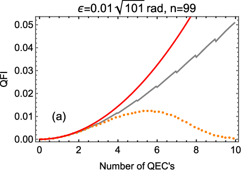
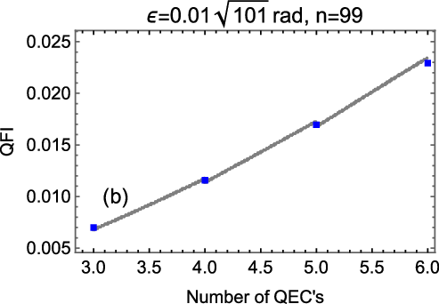
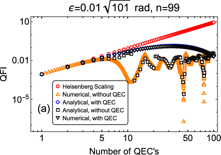
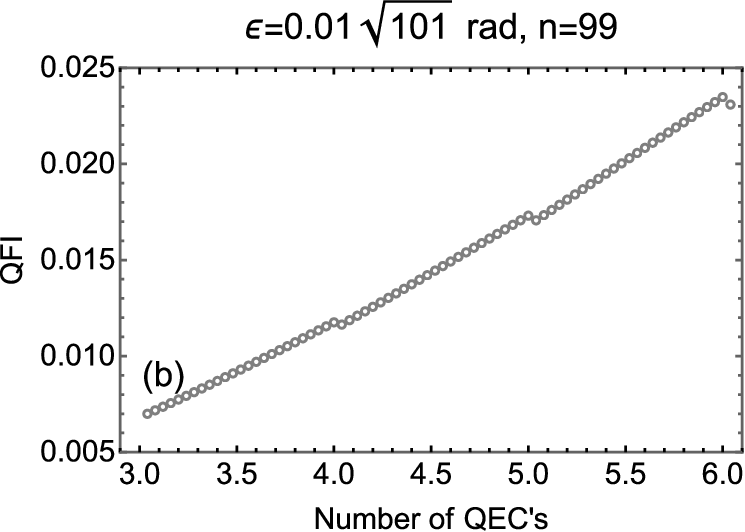
Figure 2 shows the approximation results for $\delta$ measurement and Fig. 3 shows the results from numerical simulation for comparison purposes. To summarize, the QECs significantly improve the QFI gained, confirmed in both the numerical and the analytical cases.

In general, the shorter the period $\epsilon$ of QECs is, the better the effect is. If we define the error rate as the rate that at least one error occurs, $\varepsilon(\epsilon)=(1-4\rho_{11}(\epsilon))/\epsilon,$ then for the $s$-atoms case and under the limit $\epsilon\to 0$ we obtain

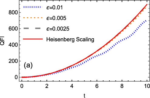
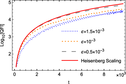
which means the error rate decreases linearly as $\epsilon$ decreases. We see this more evidently in Fig. 4(a) and Fig. 4(b). It is worth noting that in a noisy environment where $n$ is large, the correcting period $\epsilon$ has to be shortened accordingly for $\varepsilon\propto n\epsilon$ to remain constant.

If we have $s$ atoms where $s>3$, the dimension of the Hilbert space will be $2^{s}$, which can be reduced to $s+1$ by the same aforementioned method. The corresponding $s$-qubit QEC is made such that any wrongly flipped qubits shall be unflipped according to the majority rule, assuming that the QEC is fast enough so that less than half of the qubits are wrongly flipped. At time $t=\eta\epsilon$, there are only up to four non-zero entries in $\rho_{S}^{\prime}(\eta\epsilon)$, just as in the three-qubit case, which means that the only new terms we need to calculate are ${\rho_{S}}^{\prime}_{1,(s+1)}$ and ${\rho_{S}}^{\prime}_{(s+1),1}$. At time $t=\eta\epsilon+\tau$, the general expression of $\rho_{S}^{\prime}(\eta\epsilon+\tau)$ for the $s$-atom case can be speculated:

where $\rho_{ii}=[\rho_{S}^{\prime}(\eta\epsilon+\tau)]_{ii}$ and $u_{ij}=(U_{\text{II}}(\tau))_{ij}$. All other entries are zeros except $\rho_{1,(s+1)}$ and $\rho_{(s+1),1}$. The results can be derived from calculations similar to those in Eq. (8) and (9), where the main difficulty lies in calculating $U_{\text{II}}(\epsilon)$, even with the large $n$ approximation applied. The above speculated formula is verified for $s=2,3$ and 4 cases.

In the second method, we still consider the approximation $n\gg s$ such that $\hat{a}$ and $\hat{a}^{\dagger}$ can be treated as c-numbers $a$ and $a^{*}$, instead of operators for the moment; they will be restored to operators later. If we consider the $s$-atom case where $s$ is odd, then the original Hamiltonian [Eq. (1)] becomes

For each $i$, we have the eigenvalues $E_{\pm}=n\omega_{c}\pm\frac{1}{2}\Delta$ where $\Delta=\sqrt{n\Omega^{2}+\omega_{a}^{2}}$ and $n=|a|^{2}$, and the eigenstates $\left|\Psi_{+}\right\rangle=c_{0}|0\rangle+c_{1}|1\rangle$ and $\left|\Psi_{-}\right\rangle=-c_{1}^{*}|0\rangle+c_{0}^{*}|1\rangle$ where $c_{0}=b/\sqrt{|b|^{2}+1}$, $c_{1}=c_{0}/b,$ and $b=(\Delta-\omega_{a})/(\Omega a^{*})$. The eigenstates can be rearranged such that $\left|0\right\rangle=c_{0}^{*}\left|\Psi_{+}\right\rangle-c_{1}\left|\Psi_{-}\right\rangle$ and $\left|1\right\rangle=c_{1}^{*}\left|\Psi_{+}\right\rangle+c_{0}\left|\Psi_{-}\right\rangle$ which after time $\epsilon$, becomes

where $x_{i}(\epsilon)$ are some functions that are easily solvable.

If the initial state of the atoms is given by $\left|\psi_{0}\right\rangle=\frac{1}{\sqrt{2}}(|0\rangle^{\otimes n}+\left|1\right\rangle^{\otimes n}),$ then at time $\epsilon$ it becomes

where $P$ sums over all permutations on the $s$ atoms. We then apply QECs to unflip all wrongly flipped qubits according to the majority voting rule, $\rho(\epsilon)\stackrel{{\scriptstyle QEC}}{{\longrightarrow}}\sum_{k}\hat{Q}_{k}\rho(\epsilon)\hat{Q}_{k}^{\dagger},$ where

for all $k=0,1,2,\cdots,(s-1)/2$. After one run of QEC, the density matrix at time $\epsilon$ becomes

where $z_{0}(k,t)=x_{1}^{k}(\epsilon)x_{2}^{s-k}(\epsilon)$, $z_{1}(k,t)=x_{3}^{k}(\epsilon)x_{4}^{s-k}(\epsilon)$ and

which is written under the basis $\{\left|0\right\rangle^{\otimes s},\left|1\right\rangle^{\otimes s}\}$.

We notice that $\hat{A}(k,\epsilon)\rho_{0}\hat{A}^{\dagger}(k,\epsilon)$ can be written as a sum of $\hat{A}(k,\epsilon)\sigma_{\alpha}\hat{A}^{\dagger}(k,\epsilon)$ where $\alpha\in\{I,x,y,z\}$ (we denote $\sigma_{I}=1$),

such that

where

Here $a_{\alpha},b_{\alpha}$, and $c_{\alpha}$ are some terms that can be easily calculated.

By Eq.  (22), the corrected density matrix can then be written as $\rho^{\prime}(\epsilon)=1/2(1,~x,~y,~z)\mathcal{V}(\epsilon)\vec{\sigma},$ where $\mathcal{V}(\epsilon)=\sum_{k=(s+1)/2}^{s}V(k,\epsilon).$ The benefit of the above approach is that to know the density matrix after $\eta$ number of QECs, we only need to raise the power of $\mathcal{V}(\epsilon)$ to $\eta$, which is very handy:

It is worth noting that $\mathcal{V}(\epsilon)$ is always a $4\times 4$ matrix, no matter how many atoms we have. For the three-atom case, $\mathcal{V}(\epsilon)$ turns out to be a block matrix $\mathcal{V}(\epsilon)=1_{1\times 1}\oplus V_{3\times 3}$ with the analytic expressions of each entry explicitly obtainable, but too cumbersome to be shown here.

After obtaining $\rho^{\prime}(\eta\epsilon)$, the c-numbers $a$, $a^{*}$, and $n$ can be restored to operators. We can then calculate $\rho_{S}^{\prime}(\eta\epsilon)=\sum_{m}\left\langle m\right|\rho^{\prime}(\eta\epsilon)\left|m\right\rangle$. It would be the best if we choose the the cavity to be initially at the coherent state $\left|\alpha\right\rangle$ such that $\hat{a}|\alpha\rangle=\alpha|\alpha\rangle$ where $|\alpha|^{2}$ equals the mean number of photons. In this case, the c-numbers $a$ and $a^{*}$ can be replaced to $\sqrt{n}$ throughout the calculation, if considering the $n\gg s$ approximation such that $\hat{a}^{\dagger}\left|\alpha\right\rangle\approx\alpha^{*}\left|\alpha\right\rangle.$

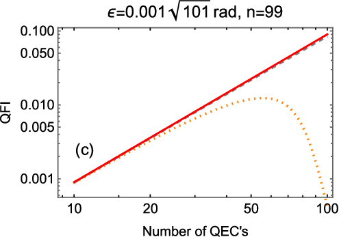
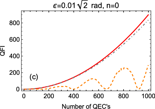
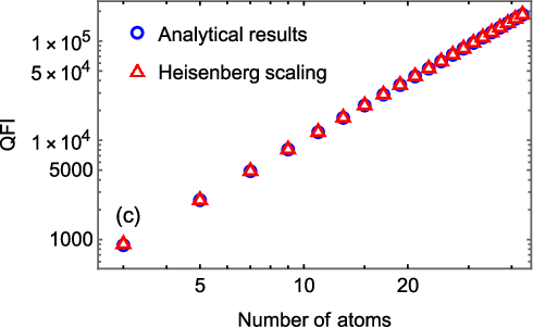
Figures 4(a) and 4(b) show QFI with different QEC frequencies, using the results from the second method. Smaller $\epsilon$ indicates more frequent QECs, which gives high QFI even in a prolonged time. Figure 4(c) showes that the Heisenberg scaling applies not only to the time $t$, but also the number of atoms $s$, i.e. $\mathcal{F_{\delta}}(s)\propto s^{2}$. Note that different from Figs. 2 and 3, we assume the cavity is initially in the coherent state $\left|\alpha\right\rangle$, instead of the Fock state $\left|n\right\rangle$.

References

- (1) V. Giovannetti, S. Lloyd, and L. Maccone, “Quantum metrology,” Physical review letters, vol. 96, no. 1, p. 010401, 2006.
- (2) V. Giovannetti, S. Lloyd, and L. Maccone, “Advances in quantum metrology,” Nature photonics, vol. 5, no. 4, pp. 222–229, 2011.
- (3) R. Schnabel, N. Mavalvala, D. E. McClelland, and P. K. Lam, “Quantum metrology for gravitational wave astronomy,” Nature communications, vol. 1, no. 1, pp. 1–10, 2010.
- (4) M. A. Taylor and W. P. Bowen, “Quantum metrology and its application in biology,” Physics Reports, vol. 615, pp. 1–59, 2016.
- (5) S. P. Nolan and S. A. Haine, “Quantum fisher information as a predictor of decoherence in the preparation of spin-cat states for quantum metrology,” Physical Review A, vol. 95, no. 4, p. 043642, 2017.
- (6) A. Valencia, G. Scarcelli, and Y. Shih, “Distant clock synchronization using entangled photon pairs,” Applied Physics Letters, vol. 85, no. 13, pp. 2655–2657, 2004.
- (7) F. Albarelli, M. Barbieri, M. G. Genoni, and I. Gianani, “A perspective on multiparameter quantum metrology: From theoretical tools to applications in quantum imaging,” Physics Letters A, vol. 384, no. 12, p. 126311, 2020.
- (8) A. N. Jordan, “Time dependent metrology: improving precision through coherent control,” in Advances in Photonics of Quantum Computing, Memory, and Communication XII, vol. 10933, p. 1093306, International Society for Optics and Photonics, 2019.
- (9) V. Giovannetti, S. Lloyd, and L. Maccone, “Quantum-enhanced measurements: beating the standard quantum limit,” Science, vol. 306, no. 5700, pp. 1330–1336, 2004.
- (10) S. F. Huelga, C. Macchiavello, T. Pellizzari, A. K. Ekert, M. B. Plenio, and J. I. Cirac, “Improvement of frequency standards with quantum entanglement,” Physical Review Letters, vol. 79, no. 20, p. 3865, 1997.
- (11) M. Holland and K. Burnett, “Interferometric detection of optical phase shifts at the heisenberg limit,” Physical review letters, vol. 71, no. 9, p. 1355, 1993.
- (12) A. Shaji and C. M. Caves, “Qubit metrology and decoherence,” Physical Review A, vol. 76, no. 3, p. 032111, 2007.
- (13) S. Alipour, M. Mehboudi, and A. Rezakhani, “Quantum metrology in open systems: dissipative cramér-rao bound,” Physical review letters, vol. 112, no. 12, p. 120405, 2014.
- (14) S. Pang and A. N. Jordan, “Optimal adaptive control for quantum metrology with time-dependent hamiltonians,” Nature communications, vol. 8, no. 1, pp. 1–9, 2017.
- (15) S. Zhou, M. Zhang, J. Preskill, and L. Jiang, “Achieving the heisenberg limit in quantum metrology using quantum error correction,” Nature communications, vol. 9, no. 1, pp. 1–11, 2018.
- (16) Y. Chen, H. Chen, J. Liu, Z. Miao, and H. Yuan, “Fluctuation-enhanced quantum metrology,” arXiv preprint arXiv:2003.13010, 2020.
- (17) R. Demkowicz-Dobrzański and L. Maccone, “Using entanglement against noise in quantum metrology,” Physical review letters, vol. 113, no. 25, p. 250801, 2014.
- (18) P. W. Shor, “Scheme for reducing decoherence in quantum computer memory,” Physical review A, vol. 52, no. 4, p. R2493, 1995.
- (19) J. Preskill, “Reliable quantum computers,” Proceedings of the Royal Society of London. Series A: Mathematical, Physical and Engineering Sciences, vol. 454, no. 1969, pp. 385–410, 1998.
- (20) A. Y. Kitaev, “Quantum computations: algorithms and error correction,” Russian Mathematical Surveys, vol. 52, no. 6, p. 1191, 1997.
- (21) E. Knill, R. Laflamme, and W. H. Zurek, “Resilient quantum computation,” Science, vol. 279, no. 5349, pp. 342–345, 1998.
- (22) D. Gottesman, “Theory of fault-tolerant quantum computation,” Physical Review A, vol. 57, no. 1, p. 127, 1998.
- (23) D. Gottesman, “An introduction to quantum error correction and fault-tolerant quantum computation,” in Quantum information science and its contributions to mathematics, Proceedings of Symposia in Applied Mathematics, vol. 68, pp. 13–58, 2010.
- (24) E. M. Kessler, I. Lovchinsky, A. O. Sushkov, and M. D. Lukin, “Quantum error correction for metrology,” Physical review letters, vol. 112, no. 15, p. 150802, 2014.
- (25) G. Arrad, Y. Vinkler, D. Aharonov, and A. Retzker, “Increasing sensing resolution with error correction,” Physical review letters, vol. 112, no. 15, p. 150801, 2014.
- (26) R. Ozeri, “Heisenberg limited metrology using quantum error-correction codes,” arXiv preprint arXiv:1310.3432, 2013.
- (27) X.-M. Lu, S. Yu, and C. Oh, “Robust quantum metrological schemes based on protection of quantum fisher information,” Nature communications, vol. 6, no. 1, pp. 1–7, 2015.
- (28) W. Dür, M. Skotiniotis, F. Froewis, and B. Kraus, “Improved quantum metrology using quantum error correction,” Physical Review Letters, vol. 112, no. 8, p. 080801, 2014.
- (29) M. Tavis and F. W. Cummings, “Exact solution for an n-molecule—radiation-field hamiltonian,” Physical Review, vol. 170, no. 2, p. 379, 1968.
- (30) M. Tavis and F. W. Cummings, “Approximate solutions for an n-molecule-radiation-field hamiltonian,” Physical Review, vol. 188, no. 2, p. 692, 1969.
- (31) S. Agarwal, S. H. Rafsanjani, and J. Eberly, “Tavis-cummings model beyond the rotating wave approximation: Quasidegenerate qubits,” Physical Review A, vol. 85, no. 4, p. 043815, 2012.
- (32) D. M. Greenberger, M. A. Horne, and A. Zeilinger, “Going beyond bell’s theorem,” in Bell’s theorem, quantum theory and conceptions of the universe, pp. 69–72, Springer, 1989.
- (33) S. Knysh, V. N. Smelyanskiy, and G. A. Durkin, “Scaling laws for precision in quantum interferometry and the bifurcation landscape of the optimal state,” Physical Review A, vol. 83, no. 2, p. 021804, 2011.
- (34) J. Liu, X. Jing, X. Wang, et al., “Phase-matching condition for enhancement of phase sensitivity in quantum metrology,” Physical Review A, vol. 88, no. 4, p. 042316, 2013.
- (35) J. Liu, H. Yuan, X.-M. Lu, and X. Wang, “Quantum fisher information matrix and multiparameter estimation,” Journal of Physics A: Mathematical and Theoretical, vol. 53, no. 2, p. 023001, 2019.