跳到论文正文
W Papers独立论文阅读器 arXiv:2203.00986 论文正文 计算阅读时间 · 0%
引用这篇论文根据当前论文元数据生成,正式投稿前建议核对。


License: CC BY 4.0
arXiv:2203.00986v1 [math.NA] 02 Mar 2022

Implicit/explicit, BEM/FEM coupled scheme for acoustic waves with the wave equation in the second order formulation

Lehel Banjai Note:  Maxwell Institute for Mathematical Sciences, School of Mathematical & Computer Sciences; Heriot-Watt University, Edinburgh EH14 4AS, UK Affiliation: In memory of a dear friend Francisco Javier Sayas
Abstract

Acoustic scattering of waves by bounded inhomogeneities in an unbounded homogeneous domain is considered. A symmetric coupled system of time-domain boundary integral equations and the second order formulation of the wave equation is described. A fully discrete system consists of spatial discretization by boundary and finite element methods (BEM/FEM), leapfrog time-stepping in the interior, and convolution quadrature for the boundary integral equations. Convolution quadrature is based on BDF2, trapezoidal rule, or a newly introduced truncated trapezoidal rule that has some favourable properties for both the implementation and quality of approximate solution. We give a stability and convergence analysis under a CFL conditon of the fully discrete system. The theoretical results are illustrated by numerical experiments in two dimensions.

1 Introduction

We consider the numerical simulation of the scattering of acoustic waves by a bounded inhomogeneity immersed in an infinite homogeneous domain. A time-domain boundary integral formulation (TBIE) will be used in the unbounded homogeneous domain and will be coupled with the non-homogeneous wave equation (PDE) in the interior. In space we discretize the TBIE and PDE by the boundary element and finite element methods respectively (BEM/FEM). The main aim and novelty of the paper is to present a new discretization using a second order formulation of the wave equation in the interior, explicit time-discretization of the PDE in the interior and implicit discretization of the BIE in the exterior and to prove stability and convergence of the scheme. Previous approaches have either used the first order formulation [1, 7], or a single implicit time-discretization for the interior and exterior equations [17, 14, 15], or have not given a complete error analysis [14, 15, 26]. The reason for using different discretizations for the integral and PDE is the efficiency of the explicit time-discretization in the interior and the stability of the implicit scheme in the exterior. Note that the implicit time-discretization of the exterior problem is equivalent to convolution quadrature of the time-domain boundary integral operators; see [21]. We should say that the Johnson-Nédélec non-symmetric coupling [18] while cheaper to implement and showing good performance in numerical experiments [14, 15], has so far escaped the analysis in the time-domain.

There are many works on numerical methods for time-domain boundary integral equations and the wave equation; see the review [11] for TDBIE and the recent book [10] for discretizations of the wave equation. However, there are but a few works on the coupling in the time-domain; see previous paragraph. The earlier work [7] is closest to the method developed here. While [7] analysed only BDF2 based discretization for the exterior problem we allow other second order, A-stable linear multistep methods. Furthermore, we introduce a new time-discretization with many of the good properties of the trapezoidal scheme, but more easily implemented. However, the main novelty is that we now use the second order formulation of the wave equation which allows for both simpler formulation and implementation.

We next give the statement of the problem and then proceed to introducing time-domain boundary integral operators and giving the weak formulation of the coupled system. In Section 4 we describe time discretization of TDBIE by convolution quadrature. Section 5 is central to the paper where a full stability and convergence analysis is given. In Section 6 we say a few words about the implementation and the choice of linear multistep method underlying the convolution quadrature. Finally we conclude with numerical experiments supporting the theory.

2 Statement of the problem

Let Ωj⊂ℝd\Omega_{j}\subset\mathbb{R}^{d}, j=1,…,Jj=1,\dots,J, be open, bounded, connected Lipschitz domains such that their closures do not intersect and d=2,3d=2,3 is the spatial dimension. The inhomogeneity will be contained in Ω−=∪j=1JΩj\Omega^{-}=\cup_{j=1}^{J}\Omega_{j}, Ω+=ℝd∖Ω−¯\Omega^{+}=\mathbb{R}^{d}\setminus\overline{\Omega^{-}} is the exterior domain, and Γ=∂Ω−\Gamma=\partial\Omega^{-} the boundary separating them; to simplify the notation we will often write Ω\Omega for Ω−\Omega^{-}. The wave speed inside Ω−\Omega^{-} can be variable c⁡(x):Ω−→ℝc(x)\colon\Omega^{-}\rightarrow\mathbb{R} with c∈L∞​(Ω−)c\in L^{\infty}(\Omega^{-}), c>0c>0 and ‖c‖L∞​(Ω−)<c1\|c\|_{L^{\infty}(\Omega^{-})}<c_{1} for some constant c1>0c_{1}>0. The diffusion coefficient is denoted by κ:Ω−→ℝsymd×d\kappa\colon\Omega^{-}\rightarrow\mathbb{R}_{\text{sym}}^{d\times d}, where ℝsymd×d\mathbb{R}_{\text{sym}}^{d\times d} is the space of symmetric real matrices and we assume that there exists a constant κ0>0\kappa_{0}>0 such that

ξT​κ​(x)​ξ≥κ0​|ξ|2for all ​x∈Ω−,ξ∈ℝd.\xi^{T}\kappa(x)\xi\geq\kappa_{0}|\xi|^{2}\quad\text{for all }x\in\Omega^{-},\;\xi\in\mathbb{R}^{d}.

Furthermore, ‖κ⁡(x)‖2≤κ1\|\kappa(x)\|_{2}\leq\kappa_{1} for some constant κ1>0\kappa_{1}>0 where we used the Euclidean matrix norm.

We also require the Sobolev spaces

Hℒκ1​(Ω−)={u∈H1(Ω−):div(κ∇u)∈L2(Ω−)},HΔ1​(Ω+)={u∈H1​(Ω+):Δ​u∈L2​(Ω+)}.\begin{split}H_{\mathcal{L}_{\kappa}}^{1}(\Omega^{-})&=\{u\in H^{1}(\Omega^{-})\,:\,\operatorname{div}(\kappa\nabla u)\in L^{2}(\Omega^{-})\},\\ H_{\Delta}^{1}(\Omega^{+})&=\{u\in H^{1}(\Omega^{+})\,:\,\Delta u\in L^{2}(\Omega^{+})\}.\end{split} (1)

The exterior unit normal is denoted by ν∈L∞​(Γ)\nu\in L^{\infty}(\Gamma), the trace operators are denoted by γ±:H1​(Ω±)→H1/2​(Γ)\gamma^{\pm}\colon H^{1}(\Omega^{\pm})\rightarrow H^{1/2}(\Gamma) and the normal trace operators by ∂ν+⋅=ν.(∇⋅):HΔ1(Ω+)→H−1/2(Γ)\partial^{+}_{\nu}\cdot=\nu.(\nabla\cdot)\colon H_{\Delta}^{1}(\Omega^{+})\rightarrow H^{-1/2}(\Gamma) and ∂κ,ν−⋅=ν.(κ∇⋅):Hℒκ1(Ω−)→H−1/2(Γ)\partial^{-}_{\kappa,\nu}\cdot=\nu.(\kappa\nabla\cdot)\colon H_{\mathcal{L}_{\kappa}}^{1}(\Omega^{-})\rightarrow H^{-1/2}(\Gamma).

Further, we denote by ∥⋅∥Ω±\|\cdot\|_{\Omega^{\pm}} the L2​(Ω±)L^{2}(\Omega^{\pm}) norm. The L2L^{2}-sesquilinear products over Ω\Omega and Γ\Gamma are denoted by

(u,v)Ω:=∫Ωu​v¯⟨φ,ψ⟩Γ=∫Γφ​ψ¯.\left(u,v\right)_{\Omega}:=\int_{\Omega}u\overline{v}\qquad\left\langle\varphi,\psi\right\rangle_{\Gamma}=\int_{\Gamma}\varphi\overline{\psi}.

These products can be extended in the usual way to duality products H1​(Ω)×(H1​(Ω))′H^{1}(\Omega)\times(H^{1}(\Omega))^{\prime} and H1/2(Γ)×H−1/2(Γ)H^{1/2}(\Gamma)\times H^{-1/2}(\Gamma) or H−1/2(Γ)×H1/2(Γ)H^{-1/2}(\Gamma)\times H^{1/2}(\Gamma). Finally the norms of the Hilbert spaces H−1/2(Γ)H^{-1/2}(\Gamma) and H1/2​(Γ)H^{1/2}(\Gamma) are denoted by

∥⋅∥−1/2,Γ:=∥⋅∥H−1/2(Γ)∥⋅∥1/2,Γ:=∥⋅∥H1/2​(Γ).\|\cdot\|_{-1/2,\Gamma}:=\|\cdot\|_{H^{-1/2}(\Gamma)}\qquad\|\cdot\|_{1/2,\Gamma}:=\|\cdot\|_{H^{1/2}(\Gamma)}.

Where the mapping properties of an operator are clear, we may use ∥⋅∥\|\cdot\| to denote the natural norm.

Let uincu^{\text{inc}} be the incident wave satisfying

∂t2uinc−Δ​uinc=0in ​Ω+×[0,T].\partial_{t}^{2}u^{\text{inc}}-\Delta u^{\text{inc}}=0\qquad\text{in }\Omega^{+}\times[0,T]. (2)

We assume that the supports of uinc​(0)u^{\text{inc}}(0) and ∂tuinc​(0)\partial_{t}u^{\text{inc}}(0) are contained in Ω+\Omega^{+} and that the initial energy is finite, i.e., 12​‖∂tuinc​(0)‖L2​(Ω+)2+12​‖∇uinc​(0)‖L2​(Ω+)2<∞\frac{1}{2}\|\partial_{t}u^{\text{inc}}(0)\|^{2}_{L^{2}(\Omega^{+})}+\frac{1}{2}\|\nabla u^{\text{inc}}(0)\|^{2}_{L^{2}(\Omega^{+})}<\infty. The total field utotu^{\text{tot}} satisfies the homogeneous wave equation in the exterior domain

∂t2utot−Δ​utot=0in ​Ω+×[0,T]\partial_{t}^{2}u^{\text{tot}}-\Delta u^{\text{tot}}=0\qquad\text{in }\Omega^{+}\times[0,T] (3)

and the non-homogeneous wave equation in the interior

1c2∂t2utot−div(κ∇utot)=fin Ω−×[0,T],\frac{1}{c^{2}}\partial_{t}^{2}u^{\text{tot}}-\operatorname{div}(\kappa\nabla u^{\text{tot}})=f\qquad\text{in }\Omega^{-}\times[0,T], (4)

where the support of f⁡(t)∈L2​(Ω−)f(t)\in L^{2}(\Omega^{-}) is contained in Ω−\Omega^{-} for all t∈[0,T]t\in[0,T]. The system is completed by transmission conditions on Γ\Gamma

γ+​utot=γ−​utot,∂ν+utot=∂κ,ν−utot\gamma^{+}u^{\text{tot}}=\gamma^{-}u^{\text{tot}},\qquad\partial_{\nu}^{+}u^{\text{tot}}=\partial^{-}_{\kappa,\nu}u^{\text{tot}} (5)

and initial conditions

utot(0)=uinc(0),∂tutot(0)=∂tuinc(0) in Ω+u^{\text{tot}}(0)=u^{\text{inc}}(0),\;\partial_{t}u^{\text{tot}}(0)=\partial_{t}u^{\text{inc}}(0)\qquad\text{ in }\Omega^{+} (6)

and

utot(0)=u0,∂tutot(0)=v0 in Ω−,u^{\text{tot}}(0)=u_{0},\;\partial_{t}u^{\text{tot}}(0)=v_{0}\qquad\text{ in }\Omega^{-}, (7)

for given initial data u0u_{0} and v0v_{0} with supports contained in Ω−\Omega^{-}. Note that due to the assumptions on uincu^{\text{inc}}, u0u_{0}, and v0v_{0}, utot​(0)u^{\text{tot}}(0) and ∂tutot​(0)\partial_{t}u^{\text{tot}}(0) are zero in a neighbourhood of Γ\Gamma.

In the exterior, as is common, instead of utotu^{\text{tot}} we will be computing the scattered field

u+=utot−uincin ​Ω+.u^{+}=u^{\text{tot}}-u^{\text{inc}}\qquad\text{in }\Omega^{+}. (8)

Furthermore, to simplify notation, we denote the total field in the interior by

u=utotin ​Ω−.u=u^{\text{tot}}\qquad\text{in }\Omega^{-}. (9)
Refer to caption
Figure 1: The geometrical setting of the coupling problem.

Putting everything together we are solving the following problem: Find u⁡(t)∈Hℒκ1​(Ω−)u(t)\in H_{\mathcal{L}_{\kappa}}^{1}(\Omega^{-}), u+​(t)∈HΔ1​(Ω+)u^{+}(t)\in H_{\Delta}^{1}(\Omega^{+}) such that for t∈[0,T]t\in[0,T]

c−2∂t2u−div(κ∇u)=fin Ω−,c^{-2}\partial_{t}^{2}u-\operatorname{div}(\kappa\nabla u)=f\qquad\text{in }\Omega^{-}, (10a)
∂t2u+−Δ​u+=0in ​Ω+,\partial_{t}^{2}u^{+}-\Delta u^{+}=0\qquad\text{in }\Omega^{+}, (10b)
γ−​u=γ+​u++β0on ​Γ,\gamma^{-}u=\gamma^{+}u^{+}+\beta_{0}\qquad\text{on }\Gamma, (10c)
∂κ,ν−u=∂ν−u++β1on ​Γ,\partial_{\kappa,\nu}^{-}u=\partial_{\nu}^{-}u^{+}+\beta_{1}\qquad\text{on }\Gamma, (10d)

where β0=γ+​uinc\beta_{0}=\gamma^{+}u^{\text{inc}} and β1=∂νuinc\beta_{1}=\partial_{\nu}u^{\text{inc}} are the traces of the incident wave onto Γ\Gamma; see Figure 1. As at time t=0t=0, uincu^{\text{inc}} has not reached the domain Ω−\Omega^{-}, u+u^{+} satisfies the zero initial condition

u+​(0)=∂tu+​(0)=0 in ​Ω+.u^{+}(0)=\partial_{t}u^{+}(0)=0\qquad\text{ in }\Omega^{+}.

and uu the inital condition

u(0)=u0,∂tu(0)=v0in Ω−.u(0)=u_{0},\;\partial_{t}u(0)=v_{0}\qquad\text{in }\Omega^{-}.

The smoothness requirements in time of the data uincu^{\text{inc}} and ff will be given in the next section once we describe the boundary-field formulation of the problem.

3 One sided time-convolutions and time-domain boundary integral operators

We intend to represent the solution in the unbounded domain by time-domain boundary integral potentials. To introduce some notation and properties of these we first consider the one-sided convolution

K(∂t)g(t)=∫0tk(t−τ)g(τ)dτ,K(\partial_{t})g(t)=\int_{0}^{t}k(t-\tau)g(\tau)d\tau,

where the kernel kk is given via its Laplace transform

K⁡(s)=ℒ​{k}​(s)=∫0∞e−s​t​K​(s)​𝑑sRe⁡s>0.K(s)=\mathscr{L}\{k\}(s)=\int_{0}^{\infty}e^{-st}K(s)ds\qquad\operatorname{Re}s>0.

If the kernel kk and the data gg are integrable, the meaning of the convolution is clear. However often this is not the case and instead we only know that KK is analytic for Re⁡s>0\operatorname{Re}s>0 and satisfies the bound

|K⁡(s)|≤C⁡(σ)​|s|μ,∀Re⁡s≥σ>0.|K(s)|\leq C(\sigma)|s|^{\mu},\qquad\forall\operatorname{Re}s\geq\sigma>0. (11)

In this case, following [21], the convolution is defined by

K(∂t)g(t):=ℒ−1{KG}(t)=12​π​i∫σ+i​ℝes​tK(s)G(s)ds,K(\partial_{t})g(t):=\mathscr{L}^{-1}\{KG\}(t)=\frac{1}{2\pi\mathrm{i}}\int_{\sigma+\mathrm{i}\mathbb{R}}e^{st}K(s)G(s)ds,

where GG is the Laplace transform of data gg, ℒ−1\mathscr{L}^{-1} is the inverse Laplace transform, and the operational notation K(∂t)K(\partial_{t}) emphasizes the importance of the kernel in the Laplace domain. Note that if g∈Cm​([0,∞))g\in C^{m}([0,\infty)) and its derivatives upto order mm are polynomially bounded with g⁡(0)=g′​(0)=⋯=g(m−1)​(0)=0g(0)=g^{\prime}(0)=\dots=g^{(m-1)}(0)=0, then

|ℒ​g​(s)|≤|s|−m​∫0∞e−σ​t​g(m)​(t)​𝑑t.\left|\mathscr{L}g(s)\right|\leq|s|^{-m}\int_{0}^{\infty}e^{-\sigma t}g^{(m)}(t)dt.

If m>μ+1m>\mu+1, the inverse Laplace transform and the Cauchy integral formula imply that K(∂t)g∈C([0,∞))K(\partial_{t})g\in C([0,\infty)) and K(∂t)g(0)=0K(\partial_{t})g(0)=0. If gg is only defined on a finite interval [0,T][0,T], we can extend it by the Taylor polynomial ∑j=0m1j!​g(j)​(T)​(t−T)m\sum_{j=0}^{m}\frac{1}{j!}g^{(j)}(T)(t-T)^{m} to t>Tt>T and again define K(∂t)gK(\partial_{t})g via the Laplace domain as above.

For K⁡(s)=sK(s)=s and sufficiently smooth gg, K(∂t)g=∂tgK(\partial_{t})g=\partial_{t}g is indeed the time-derivative justifying the operational notation. Furthermore, for sufficiently smooth gg and operators K1K_{1} and K2K_{2} satisfying bound of the form (11), the composition property K2K1(∂t)g=K2(∂t)K1(∂t)gK_{2}K_{1}(\partial_{t})g=K_{2}(\partial_{t})K_{1}(\partial_{t})g holds.

The theory of time domain boundary integral operators seemlesly fits into this framework; see [21]. Namely, the Laplace domain single layer and double layer potentials are given by

S⁡(s)​φ​(x):=∫Γ𝒦⁡(|x−y|,s)​φ​(y)​d​Γyx∈ℝd∖ΓS(s)\varphi(x):=\int_{\Gamma}\mathcal{K}(|x-y|,s)\varphi(y)d\Gamma_{y}\qquad x\in\mathbb{R}^{d}\setminus\Gamma

and

D⁡(s)​φ​(x):=∫Γ[∂νy𝒦⁡(|x−y|,s)]​φ​(y)​d​Γyx∈ℝd∖Γ,D(s)\varphi(x):=\int_{\Gamma}\left[\partial_{\nu_{y}}\mathcal{K}(|x-y|,s)\right]\varphi(y)d\Gamma_{y}\qquad x\in\mathbb{R}^{d}\setminus\Gamma,

with the kernel 𝒦⁡(r,s)\mathcal{K}(r,s) given by

𝒦⁡(r,s):={12​π​K0​(s​r)d=2e−s​r4​π​rd=3.,\mathcal{K}(r,s):=\left\{\begin{array}[]{cc}\displaystyle\frac{1}{2\pi}K_{0}(sr)&d=2\\ \displaystyle\frac{e^{-sr}}{4\pi r}&d=3.\end{array}\right.,

where K0​(⋅)K_{0}(\cdot) is a modified Bessel function [23, Chapter 10]. The single and double-layer potentials have the mapping properties

S(s):H−1/2(Γ)→H1(ℝd∖Γ),D(s):H1/2(Γ)→H1(ℝd∖Γ)S(s)\colon H^{-1/2}(\Gamma)\to H^{1}(\mathbb{R}^{d}\setminus\Gamma),\qquad D(s)\colon H^{1/2}(\Gamma)\to H^{1}(\mathbb{R}^{d}\setminus\Gamma)

and satisfy bounds

‖S⁡(s)‖≤C⁡(σ)​|s|Re⁡s,‖D⁡(s)‖≤C⁡(σ)​|s|3/2Re⁡s,Re⁡s≥σ>0.\|S(s)\|\leq C(\sigma)\frac{|s|}{\operatorname{Re}s},\quad\|D(s)\|\leq C(\sigma)\frac{|s|^{3/2}}{\operatorname{Re}s},\qquad\operatorname{Re}s\geq\sigma>0.

For these and other estimates in the Laplace domain see the original papers of Bamberger and Ha Duong [2, 3], crucial progress made in [19] and the books [8, 25].

Hence, as described in the discussion on one-sided convolutions, the time-domain single layer and double layer time domain boundary integral potentials S(∂t)S(\partial_{t}) and D(∂t)D(\partial_{t}) are well-defined. For sufficiently smooth data φ\varphi, ψ\psi they are given by the explicit formula

S(∂t)φ(x,t):=∫0t∫Γk(|x−y|,t−τ)φ(y,τ)dΓydτx∈ℝd∖ΓS(\partial_{t})\varphi(x,t):=\int_{0}^{t}\int_{\Gamma}k(|x-y|,t-\tau)\varphi(y,\tau)d\Gamma_{y}d\tau\qquad x\in\mathbb{R}^{d}\setminus\Gamma

and

D(∂t)ψ(x,t):=∫0t∫Γ[∂νyk(|x−y|,t−τ)]ψ(y,τ)dΓydτx∈ℝd∖Γ,D(\partial_{t})\psi(x,t):=\int_{0}^{t}\int_{\Gamma}\left[\partial_{\nu_{y}}k(|x-y|,t-\tau)\right]\psi(y,\tau)d\Gamma_{y}d\tau\qquad x\in\mathbb{R}^{d}\setminus\Gamma,

where the kernel kk is given by

k⁡(r,t):={H⁡(t−r)2​π​t2−r2d=2δ⁡(t−r)4​π​rd=3,k(r,t):=\left\{\begin{array}[]{cc}\displaystyle\frac{H(t-r)}{2\pi\sqrt{t^{2}-r^{2}}}&d=2\\ \displaystyle\frac{\delta(t-r)}{4\pi r}&d=3,\end{array}\right.

and δ⁡(⋅)\delta(\cdot) and H⁡(⋅)H(\cdot) are the Dirac delta and Heaviside distributions respectively. Note that the kernel of the Laplace domain operators 𝒦\mathcal{K} is the Laplace transform of kk.

If UU solves the Laplace transformed wave equation

s2​U−Δ​U=0in ​Ω+,s^{2}U-\Delta U=0\qquad\text{in }\Omega^{+},

then Kirchhoff’s representation formula gives uu in terms of boundary integral potentials

U=−S(s)∂ν+U+D(s)γ+U.U=-S(s)\partial_{\nu}^{+}U+D(s)\gamma^{+}U.

The corresponding formula holds in the time-domain, and we represent u+u^{+} as a combination of boundary integral potentials using the Kirchhoff formula

u+=S(∂t)φ+∂t−1D(∂t)ψ,u^{+}=S(\partial_{t})\varphi+\partial_{t}^{-1}D(\partial_{t})\psi, (12)

where the densities are exterior traces of the scattered field

φ=−∂+νu+,ψ=γ+∂tu+.\varphi=-\partial^{+}_{\nu}u^{+},\qquad\psi=\gamma^{+}\partial_{t}u^{+}. (13)

The densities φ\varphi and ψ\psi will be the unkowns in addition to the interior solution uu. The reason for using this particular form of the densities φ\varphi and ψ\psi will will only become apparent once we obtain a convenient boundary-field formulation of the transmission problem.

Next, by taking appropriate traces of the boundary potentials we obtain the boundary integral operators. First, we define the boundary average

{{⋅}}=12(γ+⋅+γ−⋅)\left\{\!\!\left\{\cdot\right\}\!\!\right\}=\tfrac{1}{2}(\gamma^{+}\cdot+\gamma^{-}\cdot)

and the boundary jump

[[⋅]]=γ+⋅−γ−⋅\left[\!\left[\cdot\right]\!\right]=\gamma^{+}\cdot-\gamma^{-}\cdot

and recall the jump properties of the layer potentials

[[S(∂t)φ]]=0,[[∂νS(∂t)φ]]=−φ,[[D(∂t)ψ]]=ψ,[[∂νD(∂t)ψ]]=0.\begin{split}\left[\!\left[S(\partial_{t})\varphi\right]\!\right]&=0,\\ \left[\!\left[\partial_{\nu}S(\partial_{t})\varphi\right]\!\right]&=-\varphi,\\ \left[\!\left[D(\partial_{t})\psi\right]\!\right]&=\psi,\\ \left[\!\left[\partial_{\nu}D(\partial_{t})\psi\right]\!\right]&=0.\end{split} (14)

Finally we define four boundary integral operators

V(∂t)φ={{S(∂t)φ}}=γ±S(∂t)φK(∂t)ψ={{D(∂t)ψ}}Kt(∂t)φ={{∂νS(∂t)φ}}W(∂t)ψ=−{{∂νD(∂t)ψ}}=−∂±νD(∂t)\begin{split}V(\partial_{t})\varphi&=\left\{\!\!\left\{S(\partial_{t})\varphi\right\}\!\!\right\}=\gamma^{\pm}S(\partial_{t})\varphi\\ K(\partial_{t})\psi&=\left\{\!\!\left\{D(\partial_{t})\psi\right\}\!\!\right\}\\ K^{t}(\partial_{t})\varphi&=\left\{\!\!\left\{\partial_{\nu}S(\partial_{t})\varphi\right\}\!\!\right\}\\ W(\partial_{t})\psi&=-\left\{\!\!\left\{\partial_{\nu}D(\partial_{t})\psi\right\}\!\!\right\}=-\partial^{\pm}_{\nu}D(\partial_{t})\end{split}

where VV, KK, KtK^{t}, WW are the single layer, double layer, transposed double layer and hypersingular boundary integral operators. Note that

V⁡(s):H−1/2(Γ)→H1/2(Γ)K⁡(s):H1/2​(Γ)→H1/2​(Γ)Kt​(s):H−1/2(Γ)→H−1/2(Γ)W⁡(s):H1/2(Γ)→H−1/2(Γ)\begin{split}V(s)\colon&H^{-1/2}(\Gamma)\rightarrow H^{1/2}(\Gamma)\\ K(s)\colon&H^{1/2}(\Gamma)\rightarrow H^{1/2}(\Gamma)\\ K^{t}(s)\colon&H^{-1/2}(\Gamma)\rightarrow H^{-1/2}(\Gamma)\\ W(s)\colon&H^{1/2}(\Gamma)\rightarrow H^{-1/2}(\Gamma)\end{split}

and that each of the operators satisfies a bound of the form (11) with μ=1,3/2,3/2,2\mu=1,3/2,3/2,2 respectively; see [25].

The above definitions and jump properties imply

γ+D(∂t)ψ=12ψ+K(∂t)ψ\gamma^{+}D(\partial_{t})\psi=\frac{1}{2}\psi+K(\partial_{t})\psi

and

∂ν+S(∂t)φ=−12φ+Kt(∂t)φ.\partial_{\nu}^{+}S(\partial_{t})\varphi=-\frac{1}{2}\varphi+K^{t}(\partial_{t})\varphi.

In particular, differentiating (12) in time, taking the trace gives

γ+∂tu+=∂tV(∂t)φ+12ψ+K(∂t)ψ\gamma^{+}\partial_{t}u^{+}=\partial_{t}V(\partial_{t})\varphi+\frac{1}{2}\psi+K(\partial_{t})\psi

and applying the transmission condition (10d)

−∂tβ0=−γ−∂tu++∂tV(∂t)φ+12ψ+K(∂t)ψ.-\partial_{t}\beta_{0}=-\gamma^{-}\partial_{t}u^{+}+\partial_{t}V(\partial_{t})\varphi+\frac{1}{2}\psi+K(\partial_{t})\psi. (15)

Further, taking the normal trace of (12) gives

−12φ−Kt(∂t)φ+∂t−1W(∂t)ψ=0.-\frac{1}{2}\varphi-K^{t}(\partial_{t})\varphi+\partial_{t}^{-1}W(\partial_{t})\psi=0. (16)

Finally, testing the strong formulation (10a) in the interior by v∈H1​(Ω−)v\in H^{1}(\Omega^{-}) and using the transmission condition (10d) we obtain the weak formulation in the interior

(c−2∂t2u,v)Ω+(κ∇u,∇v)Ω+⟨φ,γ−v⟩Γ=(f,v)Ω+⟨β1,γ−v⟩Γ.\left(c^{-2}\partial_{t}^{2}u,v\right)_{\Omega}+\left(\kappa\nabla u,\nabla v\right)_{\Omega}+\left\langle\varphi,\gamma^{-}v\right\rangle_{\Gamma}=\left(f,v\right)_{\Omega}+\left\langle\beta_{1},\gamma^{-}v\right\rangle_{\Gamma}.

Thus, combining this with the boundary integral equations (15) and (16), the boundary/field formulation of the scattering problem reads: Find u⁡(t)∈Hℒκ1​(Ω−)u(t)\in H_{\mathcal{L}_{\kappa}}^{1}(\Omega^{-}), φ∈H−1/2(Γ)\varphi\in H^{-1/2}(\Gamma), ψ∈H1/2​(Γ)\psi\in H^{1/2}(\Gamma) such that for almost all t∈[0,T]t\in[0,T]

(c−2∂t2u,v)Ω+(κ∇u,∇v)Ω+⟨φ,γ−v⟩Γ=(f,v)Ω+⟨β1,γ−v⟩Γ\left(c^{-2}\partial_{t}^{2}u,v\right)_{\Omega}+\left(\kappa\nabla u,\nabla v\right)_{\Omega}+\left\langle\varphi,\gamma^{-}v\right\rangle_{\Gamma}=\left(f,v\right)_{\Omega}+\left\langle\beta_{1},\gamma^{-}v\right\rangle_{\Gamma} (17a)
(−γ−∂tu0)+(012​I−12​I0)(φψ)+B(∂t)(φψ)=(−∂tβ00)\begin{pmatrix}-\gamma^{-}\partial_{t}u\\ 0\end{pmatrix}+\begin{pmatrix}0&\frac{1}{2}I\\ -\frac{1}{2}I&0\end{pmatrix}\begin{pmatrix}\varphi\\ \psi\end{pmatrix}+B(\partial_{t})\begin{pmatrix}\varphi\\ \psi\end{pmatrix}=\begin{pmatrix}-\partial_{t}\beta_{0}\\ 0\end{pmatrix} (17b)

for all v∈H1​(Ω−)v\in H^{1}(\Omega^{-}), where the second equality is understood in H1/2(Γ)×H−1/2(Γ)H^{1/2}(\Gamma)\times H^{-1/2}(\Gamma), the initial data are given by

u⁡(0)=u0​(in ​H1​(Ω−))∂tu⁡(0)=v0​(in ​L2​(Ω−)),u(0)=u_{0}\;(\text{in }H^{1}(\Omega^{-}))\qquad\partial_{t}u(0)=v_{0}\;(\text{in }L^{2}(\Omega^{-})),

and BB is the Calderón operator

B(∂t)=(∂tV(∂t)K(∂t)−Kt(∂t)∂t−1W(∂t)).B(\partial_{t})=\begin{pmatrix}\partial_{t}V(\partial_{t})&K(\partial_{t})\\ -K^{t}(\partial_{t})&\partial_{t}^{-1}W(\partial_{t})\end{pmatrix}. (18)

The bounds on the constituent operators in the definition of BB imply that the operator B(s):H−1/2(Γ)×H1/2(Γ)→H1/2(Γ)×H−1/2(Γ)B(s)\colon H^{-1/2}(\Gamma)\times H^{1/2}(\Gamma)\to H^{1/2}(\Gamma)\times H^{-1/2}(\Gamma) itself satisfies a bound of the form (11):

‖B⁡(s)‖≤C⁡(σ)​|s|2Re⁡s≥σ>0.\|B(s)\|\leq C(\sigma)|s|^{2}\qquad\operatorname{Re}s\geq\sigma>0. (19)

Next, we state a crucial property of the Calderón operator in the frequency domain; for a proof see [7].

Lemma 1.

There exists β>0\beta>0 so that the Calderón operator (18) satisfies

Re⟨(φψ),B(s)(φψ)⟩Γ≥βmin(1,|s|2)Re⁡s|s|2(∥φ∥−1/2,Γ2+∥ψ∥1/2,Γ2)\operatorname{Re}\left\langle\begin{pmatrix}\varphi\\ \psi\end{pmatrix},B(s)\begin{pmatrix}\varphi\\ \psi\end{pmatrix}\right\rangle_{\Gamma}\geq\beta\,\min(1,|s|^{2})\frac{\operatorname{Re}s}{|s|^{2}}\left(\|\varphi\|^{2}_{-1/2,\Gamma}+\|\psi\|^{2}_{1/2,\Gamma}\right)

for Re⁡s>0\operatorname{Re}s>0 and for all φ∈H−1/2(Γ)\varphi\in H^{-1/2}(\Gamma) and ψ∈H1/2​(Γ)\psi\in H^{1/2}(\Gamma).

Let us briefly consider the existence and uniqueness of the solution to the coupled system (17). Following [25], for a Banach space XX, let us denote by T​D​(X)TD(X) the space of causal, tempered distributions with polynomially bounded Laplace transform. Namely, for f∈T​D​(X)f\in TD(X), there exists a non-increasing function CF​(x)>0C_{F}(x)>0 with CF​(x)≤C​x−mC_{F}(x)\leq Cx^{-m} for some mm and x∈(0,1)x\in(0,1), such that

‖ℒ​{f}​(s)‖X≤C⁡(σ)​|s|m,Re⁡s≥σ>0.\|\mathcal{L}\{f\}(s)\|_{X}\leq C(\sigma)|s|^{m},\qquad\operatorname{Re}s\geq\sigma>0.

For vanishing ff, u0u_{0} and v0v_{0}, the existence and uniqueness of the solution of (17) can be shown by means of the Laplace transform and the above coercivity result under very weak conditions on the smoothness of the data; for details see [8, Chapter 7] and also [17, Proposition 2.1]. Namely, if β0∈T​D​(H1/2​(Γ))\beta_{0}\in TD(H^{1/2}(\Gamma)), β1∈TD(H−1/2(Γ))\beta_{1}\in TD(H^{-1/2}(\Gamma)), there exists a unique solution u∈T​D​(Hℒκ1​(Ω−))u\in TD(H_{\mathcal{L}_{\kappa}}^{1}(\Omega^{-})), φ∈TD(H−1/2(Γ))\varphi\in TD(H^{-1/2}(\Gamma)), ψ∈T​D​(H1/2​(Γ))\psi\in TD(H^{1/2}(\Gamma)) of (17).

For vanishing β0\beta_{0} and β1\beta_{1}, we first let Ω~T\tilde{\Omega}_{T} be a bounded, Lipschitz domain such that Ω−⊂Ω~T\Omega^{-}\subset\tilde{\Omega}_{T} and

dist⁡(∂Ω−,∂Ω~T)>T.\operatorname{dist}(\partial\Omega^{-},\partial\tilde{\Omega}_{T})>T.

The existence of the unique weak solution u~​(t)∈H01​(Ω~T)\tilde{u}(t)\in H^{1}_{0}(\tilde{\Omega}_{T}) of

∂t2u~+L​u~=f\partial_{t}^{2}\tilde{u}+L\tilde{u}=f\qquad

where

L​u~={−divκ∇u~in ​Ω−−Δ​u~in ​Ω+L\tilde{u}=\left\{\begin{array}[]{cc}-\operatorname{div}\kappa\nabla\tilde{u}&\text{in }\Omega^{-}\\ -\Delta\tilde{u}&\text{in }\Omega^{+}\end{array}\right.

for f∈L2​(0,T,L2​(Ω~T))f\in L^{2}(0,T;L^{2}(\tilde{\Omega}_{T})) with initial data u~​(0)=u0∈H01​(Ω~T)\tilde{u}(0)=u_{0}\in H^{1}_{0}(\tilde{\Omega}_{T}), ∂tu~​(0)=v0∈L2​(Ω~T)\partial_{t}\tilde{u}(0)=v_{0}\in L^{2}(\tilde{\Omega}_{T}) (with u0u_{0} and v0v_{0} extended by 00 to Ω~T\tilde{\Omega}_{T}) follows by classical means, see, e.g., [13]. Note that due to the finite propagation of waves and the choice of Ω~T\tilde{\Omega}_{T}, u~​(t)≡0\tilde{u}(t)\equiv 0 in a vicinity of ∂Ω~T\partial\tilde{\Omega}_{T} for t<Tt<T. Setting u=u~|Ω−u=\tilde{u}|_{\Omega^{-}}, φ=−∂+νu\varphi=-\partial^{+}_{\nu}u, and ψ=γ+​∂tu\psi=\gamma^{+}\partial_{t}u gives a solution of (17). Uniqueness again following by the Laplace transform as in [17, 8].

The above shows existence and uniquenness of the solution to the coupled problem (17). Much stronger requirements on the smoothness of both data and solution will be made in later section to analyse the convergence of numerical methods.

4 Time-discretization of time-domain boundary integral operators

Convolution quadrature (CQ) is a time-discretization of convolutions K(∂t)gK(\partial_{t})g based on an A-stable linear multistep method for symbols KK satisfying a bound (11); see [21]. Just like the one-sided convolution, it is defined via the Laplace domain. Namely, given a fixed time-step Δ​t>0{\Delta t}>0 we define

K(∂tΔ​t)g(t):=12​π​i∫σ+i​ℝes​tK(sΔ​t)G(s)ds,K(\partial_{t}^{{\Delta t}})g(t):=\frac{1}{2\pi\mathrm{i}}\int_{\sigma+\mathrm{i}\mathbb{R}}e^{st}K(s^{{\Delta t}})G(s)ds, (20)

where

sΔ​t=δ⁡(e−s​Δ​t)Δ​ts^{{\Delta t}}=\frac{\delta(e^{-s{\Delta t}})}{{\Delta t}} (21)

and δ⁡(ζ)\delta(\zeta) is a generating function of an A-stable linear multistep method. Namely, we assume that the method is of order p≥1p\geq 1

δ⁡(e−z)=z+𝒪⁡(zp+1)\delta(e^{-z})=z+\mathcal{O}(z^{p+1}) (22)

and is A-stable

Re⁡δ⁡(ζ)>0for ​|ζ|<1.\operatorname{Re}\delta(\zeta)>0\qquad\text{for }|\zeta|<1. (23)

As the Dahlquist’s second barrier tells us that p≤2p\leq 2, we will mainly be concerned with the following second order methods: the second order backward difference formula (BDF2)

δBDF2​(ζ)=(1−ζ)+12​(1−ζ)2\delta_{\text{BDF2}}(\zeta)=(1-\zeta)+\frac{1}{2}(1-\zeta)^{2}

and the trapezoidal rule

δTR​(ζ)=2​1−ζ1+ζ=∑j=0∞2−j​(1−ζ)j+1.\delta_{\text{TR}}(\zeta)=2\frac{1-\zeta}{1+\zeta}=\sum_{j=0}^{\infty}2^{-j}(1-\zeta)^{j+1}.

As we will look at another class of linear multistep methods, we state the assumptions they need to satisfy.

Assumption 1.

Let δ⁡(ζ)\delta(\zeta) satisfy (22) for p≥1p\geq 1 and (23). Furthermore, let δ⁡(ζ)\delta(\zeta) be either analytic for |ζ|≤1|\zeta|\leq 1 or be the generating function of the trapezoidal rule.

For a sufficiently smooth gg, convolution quadrature inherits the approximation property of the underlying linear mulstistep method. To present the required smoothness we need the space

W0m(ℝ)≔{g∈Cm−1​(ℝ):g≡0​ in ​(−∞,0),g polynomially bounded ,g(m)∈L1loc(ℝ)}.\begin{split}W_{0}^{m}(\mathbb{R})\coloneqq\{&g\in C^{m-1}(\mathbb{R})\;:\;g\equiv 0\text{ in }(-\infty,0),\\ &g\text{ polynomially bounded },g^{(m)}\in L^{1}_{\text{loc}}(\mathbb{R})\}.\end{split} (24)

For g∈W0m​(ℝ)g\in W_{0}^{m}(\mathbb{R}) we then have

K(∂t)g−K(∂tΔ​t)g=𝒪(Δtp),K(\partial_{t})g-K(\partial_{t}^{{\Delta t}})g=\mathcal{O}({\Delta t}^{p}),

with m>max⁡(2​μ+3,μ+4)m>\max(2\mu+3,\mu+4) for the trapezoidal rule and m>μ+p+2m>\mu+p+2 for other methods satisfying Assumption 1. For the proof of this result see [21] (not including the trapezoidal rule for μ≥0\mu\geq 0), [12] (for the trapezoidal rule), and [8] (for all the cases).

The above brief introduction to CQ does not indicate how to implement the method; for details and short codes see [8]. For our purposes here, let us just note that K(∂tΔ​t)gK(\partial_{t}^{{\Delta t}})g is given by a discrete convolution

K(∂tΔ​t)g(tn)=∑j=0nωn−j(K)g(tj).K(\partial_{t}^{{\Delta t}})g(t_{n})=\sum_{j=0}^{n}\omega_{n-j}(K)g(t_{j}).

The convolution weights ωj​(K)\omega_{j}(K) can be expressed by the contour integral

ωj​(K)=12​π​i​∮𝒞K⁡(δ⁡(ζ)/Δ​t)​ζ−j−1​𝑑ζ,\omega_{j}(K)=\frac{1}{2\pi\mathrm{i}}\oint_{\mathcal{C}}K(\delta(\zeta)/{\Delta t})\zeta^{-j-1}d\zeta,

with 𝒞\mathcal{C} a circle of radius 0<λ<10<\lambda<1. Discretizing the contour integral by the compound trapezoidal rule gives the approximation

ωj​(K)≈λ−jN+1​∑ℓ=0NK⁡(δ⁡(λ​ζN+1−ℓ)Δ​t)​ζN+1ℓ​j,\omega_{j}(K)\approx\frac{\lambda^{-j}}{N+1}\sum_{\ell=0}^{N}K\left(\frac{\delta(\lambda\zeta_{N+1}^{-\ell})}{\Delta t}\right)\zeta_{N+1}^{\ell j}, (25)

where ζN+1=e2​π​iN+1\zeta_{N+1}=e^{\frac{2\pi\mathrm{i}}{N+1}} and 0<λ<10<\lambda<1. The error commited is 𝒪⁡(λN+1)\mathcal{O}(\lambda^{N+1}) and all NN weights can be computed in 𝒪⁡(N​log⁡N)\mathcal{O}(N\log N) time using FFT. For numerical stability reasons λ\lambda is chosen greater than eps12​N+1\text{eps}^{\frac{1}{2N+1}} where eps is the machine precision; see [21, 8].

A crucial property of CQ is that it inherits the positivity property of the kind satisfied by the Calderón operator; for a proof see [7].

Theorem 1.

Let K⁡(s)K(s) be an analytic family for Re⁡s>0\operatorname{Re}s>0 of linear operators between a Hilbert space XX and its dual X′X^{\prime} satisfying the bound

‖K⁡(s)‖≤C0​(σ)​|s|μRe⁡s≥σ>0\|K(s)\|\leq C_{0}(\sigma)|s|^{\mu}\qquad\operatorname{Re}s\geq\sigma>0

for some μ∈ℝ\mu\in\mathbb{R} and any σ>0\sigma>0. Denoting by ⟨⋅,⋅⟩\langle\cdot,\cdot\rangle the duality product, let for any σ>0\sigma>0,

⟨φ,K⁡(s)​φ⟩≥C1​(σ)​‖sη​φ‖X2∀φ∈X,\langle\varphi,K(s)\varphi\rangle\geq C_{1}(\sigma)\|s^{\eta}\varphi\|_{X}^{2}\qquad\forall\varphi\in X, (26)

Re⁡s≥σ>0\operatorname{Re}s\geq\sigma>0, and C1​(x)C_{1}(x) a non-increasing function of xx, and some η∈ℝ\eta\in\mathbb{R}. Considering CQ based on δ⁡(ζ)\delta(\zeta) satisfying Assumption 1, σ​Δ​t>0\sigma{\Delta t}>0 small enough, ϱ=e−σ​Δ​t\varrho=e^{-\sigma{\Delta t}} and any finite series φj∈X\varphi_{j}\in X the following holds

∑j=0∞ϱ2​j⟨φj,K(∂tΔ​t)φ(tj)⟩≥C2(σ)∑j=0∞ϱ2​j∥(∂tΔ​t)ηφj∥X2,\sum_{j=0}^{\infty}\varrho^{2j}\left\langle\varphi_{j},K(\partial_{t}^{\Delta t})\varphi(t_{j})\right\rangle\geq C_{2}(\sigma)\sum_{j=0}^{\infty}\varrho^{2j}\|(\partial_{t}^{\Delta t})^{\eta}\varphi_{j}\|^{2}_{X},

with some positive contant C2​(σ)C_{2}(\sigma) depending on σ\sigma and the choice of δ⁡(ζ)\delta(\zeta).

A related result we will need is stated in the next lemma. It has been used in the proofs of [7], see also [8].

Lemma 2.

Under the conditions of the previous theorem, given finite sequences φj∈X\varphi_{j}\in X and ψj∈X′\psi_{j}\in X^{\prime}, and σ>0\sigma>0, for any ϱ∈(0,1)\varrho\in(0,1) the following holds

∑j=0∞ϱ2​j|⟨φj,ψj⟩|≤12∑j=0∞ϱ2​j(∥(∂tΔ​t)−1φ(tj)∥X′2+∥∂tΔ​tψ(tj)∥X2).\sum_{j=0}^{\infty}\varrho^{2j}|\langle\varphi_{j},\psi_{j}\rangle|\leq\frac{1}{2}\sum_{j=0}^{\infty}\varrho^{2j}\left(\|(\partial_{t}^{{\Delta t}})^{-1}\varphi(t_{j})\|_{X^{\prime}}^{2}+\|\partial_{t}^{{\Delta t}}\psi(t_{j})\|_{X}^{2}\right).

Both results are proved using Parseval’s formula.

5 Fully discrete system and convergence analysis

To present the full discretization it will be useful to define the second order central difference approximations of the first and second time derivative:

[D​u]n:=12​Δ​t​(un+1−un−1),[D2​u]n:=1Δ​t2​(un+1−2​un+un−1).[Du]_{n}:=\frac{1}{2{\Delta t}}(u_{n+1}-u_{n-1}),\qquad[D^{2}u]_{n}:=\frac{1}{{\Delta t}^{2}}(u_{n+1}-2u_{n}+u_{n-1}).

For the discretization in space we let Xh⊂H1​(Ω)X_{h}\subset H^{1}(\Omega), Xh−12⊂H−1/2(Γ)X_{h}^{-\frac{1}{2}}\subset H^{-1/2}(\Gamma), Xh12⊂H1/2​(Γ)X_{h}^{\frac{1}{2}}\subset H^{1/2}(\Gamma) be families of subspaces indexed by the spatial meshwidth h>0h>0. We assume that XhX_{h} satisfies the inverse inequality

∥κ1/2∇u∥Ω≤Cinvh−1∥u∥Ωfor all u∈Xh\|\kappa^{1/2}\nabla u\|_{\Omega}\leq C_{\text{inv}}h^{-1}\|u\|_{\Omega}\qquad\text{for all }u\in X_{h} (27)

for some Cinv>0C_{\text{inv}}>0.

The Galerkin discretization of the Calderón operator denoted by Bh​(s):Xh−12×Xh12→(Xh−12)′×(Xh12)′B_{h}(s)\colon X_{h}^{-\frac{1}{2}}\times X_{h}^{\frac{1}{2}}\to(X_{h}^{-\frac{1}{2}})^{\prime}\times(X_{h}^{\frac{1}{2}})^{\prime} is defined by

⟨(zw),Bh​(s)​(ημ)⟩Γ=⟨(zw),B⁡(s)​(ημ)⟩Γ∀z∈Xh−12,w∈Xh12.\left\langle\begin{pmatrix}z\\ w\end{pmatrix},B_{h}(s)\begin{pmatrix}\eta\\ \mu\end{pmatrix}\right\rangle_{\Gamma}=\left\langle\begin{pmatrix}z\\ w\end{pmatrix},B(s)\begin{pmatrix}\eta\\ \mu\end{pmatrix}\right\rangle_{\Gamma}\qquad\forall z\in X_{h}^{-\frac{1}{2}},w\in X_{h}^{\frac{1}{2}}.

Furthermore, we denote by

Πh2:H1/2(Γ)→(Xh−12)′Πh3:H−1/2(Γ)→(Xh12)′\Pi_{h}^{2}\colon H^{1/2}(\Gamma)\to(X_{h}^{-\frac{1}{2}})^{\prime}\quad\Pi_{h}^{3}\colon H^{-1/2}(\Gamma)\to(X_{h}^{\frac{1}{2}})^{\prime}

the orthogonal projectors.

The fully discrete system then reads: Find un+1h∈Xhu_{n+1}^{h}\in X_{h}, φnh∈Xh−12\varphi^{h}_{n}\in X_{h}^{-\frac{1}{2}}, ψnh∈Xh12\psi_{n}^{h}\in X_{h}^{\frac{1}{2}} for n=1,…,N−1n=1,\dots,N-1 such that

(c−2[D2uh]n,v)Ω+(κ∇uhn,∇v)Ω+⟨φnh,γ−​v⟩Γ=(f⁡(tn),v)Ω+⟨β1​(tn),γ−​v⟩Γ\begin{split}\left(c^{-2}[D^{2}u^{h}]_{n},v\right)_{\Omega}+\left(\kappa\nabla u^{h}_{n},\nabla v\right)_{\Omega}+&\left\langle\varphi^{h}_{n},\gamma^{-}v\right\rangle_{\Gamma}\\ =&\left(f(t_{n}),v\right)_{\Omega}+\left\langle\beta_{1}(t_{n}),\gamma^{-}v\right\rangle_{\Gamma}\end{split} (28a)
⟨−γ−​[D​uh]n,z⟩Γ+12​⟨ψnh,z⟩Γ−12​⟨φnh,w⟩Γ+⟨B(∂Δ​tt)(φhψh)(tn),(zw)⟩Γ=−⟨∂tΠh2β0(tn),z⟩Γ\begin{split}\left\langle-\gamma^{-}[Du^{h}]_{n},z\right\rangle_{\Gamma}&+\tfrac{1}{2}\left\langle\psi^{h}_{n},z\right\rangle_{\Gamma}-\tfrac{1}{2}\left\langle\varphi^{h}_{n},w\right\rangle_{\Gamma}\\ &+\left\langle B(\partial^{\Delta t}_{t})\begin{pmatrix}\varphi^{h}\\ \psi^{h}\end{pmatrix}(t_{n}),\begin{pmatrix}z\\ w\end{pmatrix}\right\rangle_{\Gamma}=-\left\langle\partial_{t}\Pi_{h}^{2}\beta_{0}(t_{n}),z\right\rangle_{\Gamma}\end{split} (28b)

for all v∈Xhv\in X_{h}, z∈Xh−12z\in X_{h}^{-\frac{1}{2}}, w∈Xh12w\in X_{h}^{\frac{1}{2}}. To complete the system we need to define the initial data. We set u0h=Rh​u0u_{0}^{h}=R_{h}u_{0} and using the equation in the interior we set

u1h=u0h+Δ​t​Rh​v0+12​Δ​t2​Rh​∂t2u⁡(0)=u0h+ΔtRhv0+12Δt2Rh(c2div(κ∇u0)−f(0)).\begin{split}u_{1}^{h}&=u_{0}^{h}+{\Delta t}R_{h}v_{0}+\frac{1}{2}{\Delta t}^{2}R_{h}\partial_{t}^{2}u(0)\\ &=u_{0}^{h}+{\Delta t}R_{h}v_{0}+\frac{1}{2}{\Delta t}^{2}R_{h}(c^{2}\operatorname{div}(\kappa\nabla u_{0})-f(0)).\end{split}

Here Rh:Hℒκ1​(Ω−)→XhR_{h}\colon H_{\mathcal{L}_{\kappa}}^{1}(\Omega^{-})\to X_{h} is the elliptic projector satisfying

(κ∇Rhu,∇v)Ω+(Rhu,v)Ω=(κ∇u,∇v)Ω+(u,v)Ω∀v∈Xh1.\left(\kappa\nabla R_{h}u,\nabla v\right)_{\Omega}+\left(R_{h}u,v\right)_{\Omega}=\left(\kappa\nabla u,\nabla v\right)_{\Omega}+\left(u,v\right)_{\Omega}\qquad\forall v\in X^{1}_{h}. (29)

We also set φ0h=0\varphi_{0}^{h}=0 and ψ0h=0\psi_{0}^{h}=0 since at time t=0t=0, the wave has not yet reached the boundary Γ\Gamma.

We first prove the stability of the above system under perturbations. Stability will be shown using the discrete energy in Ω−\Omega^{-}

En(uh)=12‖unh−un−1hc​Δ​t‖Ω2+12(κ∇unh,∇un−1h)Ω.E_{n}(u^{h})=\frac{1}{2}\left\|\frac{u^{h}_{n}-u^{h}_{n-1}}{c{\Delta t}}\right\|^{2}_{\Omega}+\frac{1}{2}\left(\kappa\nabla u^{h}_{n},\nabla u^{h}_{n-1}\right)_{\Omega}.

Standard calculation shows that the inverse inequality (27) implies

En​(uh)≥12​(1−14​Cinv2​c12​Δ​t2​h−2)​‖unh−un−1hc​Δ​t‖Ω2+12​‖κ1/2​∇unh+∇un−1h2‖Ω2.E_{n}(u^{h})\geq\frac{1}{2}\left(1-\frac{1}{4}C_{\text{inv}}^{2}c_{1}^{2}{\Delta t}^{2}h^{-2}\right)\left\|\frac{u^{h}_{n}-u^{h}_{n-1}}{c{\Delta t}}\right\|^{2}_{\Omega}+\frac{1}{2}\left\|\kappa^{1/2}\frac{\nabla u^{h}_{n}+\nabla u^{h}_{n-1}}{2}\right\|^{2}_{\Omega}.

Therefore under the CFL condition

Δ​t<2​hCinv​c1{\Delta t}<\frac{\sqrt{2}h}{C_{\text{inv}}c_{1}} (30)

the discrete energy is positive and

En​(uh)≥14​‖unh−un−1hc​Δ​t‖Ω2+12​‖κ1/2​∇unh+∇un−1h2‖Ω2.E_{n}(u^{h})\geq\frac{1}{4}\left\|\frac{u^{h}_{n}-u^{h}_{n-1}}{c{\Delta t}}\right\|_{\Omega}^{2}+\frac{1}{2}\left\|\kappa^{1/2}\frac{\nabla u^{h}_{n}+\nabla u^{h}_{n-1}}{2}\right\|^{2}_{\Omega}.
Theorem 2.

Let gn∈L2​(Ω)g_{n}\in L^{2}(\Omega), ρn∈H1/2​(Γ)\rho_{n}\in H^{1/2}(\Gamma), σn∈H−1/2(Γ)\sigma_{n}\in H^{-1/2}(\Gamma), n=1​…n=1\dots, and u0h,u1h∈Xhu_{0}^{h},u_{1}^{h}\in X_{h} be given. Under the CFL condition (30), Δ​t≤Δ​t0{\Delta t}\leq{\Delta t}_{0} for some fixed Δ​t0>0{\Delta t}_{0}>0 and with φ0h=ψ0h=0\varphi_{0}^{h}=\psi_{0}^{h}=0, the system, n=1,…,Nn=1,\dots,N,

(c−2[D2uh]n,v)Ω+(κ∇uhn,∇v)Ω+⟨φhn,γ−v⟩Γ=(gn,v)Ω(−γ−​[D​uh]n0)+(12​ψnh−12​φnh)+Bh(∂Δ​tt)(φhψh)(tn)=(Πh2​ρnΠh3​σn)\begin{split}\left(c^{-2}[D^{2}u^{h}]_{n},v\right)_{\Omega}+\left(\kappa\nabla u^{h}_{n},\nabla v\right)_{\Omega}+\left\langle\varphi^{h}_{n},\gamma^{-}v\right\rangle_{\Gamma}&=\left(g_{n},v\right)_{\Omega}\\ \begin{pmatrix}-\gamma^{-}[Du^{h}]_{n}\\ 0\end{pmatrix}+\begin{pmatrix}\frac{1}{2}\psi^{h}_{n}\\ -\frac{1}{2}\varphi^{h}_{n}\end{pmatrix}+B_{h}(\partial^{\Delta t}_{t})\begin{pmatrix}\varphi^{h}\\ \psi^{h}\end{pmatrix}(t_{n})&=\begin{pmatrix}\Pi_{h}^{2}\rho_{n}\\ \Pi_{h}^{3}\sigma_{n}\end{pmatrix}\end{split}

for all v∈Xhv\in X_{h} has a unique solution. Further, the following stability bound holds

EN+1+Δt∑n=0N(∥(∂tΔ​t)−1φh(tn)∥−1/2,Γ2+∥(∂tΔ​t)−1ψh(tn)∥1/2,Γ2)≤C⁡(T)​(E1+RN),\begin{split}E_{N+1}+{\Delta t}\sum_{n=0}^{N}&\left(\|(\partial_{t}^{{\Delta t}})^{-1}\varphi^{h}(t_{n})\|_{-1/2,\Gamma}^{2}+\|(\partial_{t}^{{\Delta t}})^{-1}\psi^{h}(t_{n})\|_{1/2,\Gamma}^{2}\right)\\ &\leq C(T)(E_{1}+R_{N}),\end{split}

where

RN=12​βΔt∑n=0∞ϱ2​n(∥∂tΔ​tρ(tn)∥1/2,Γ2+∥∂tΔ​tσ(tn)∥−1/2,Γ2)+Δt12c12∑n=0Nϱ2​n∥gn∥Ω2,\begin{split}R_{N}=&\frac{1}{2\beta}{\Delta t}\sum_{n=0}^{\infty}\varrho^{2n}\left(\|\partial_{t}^{{\Delta t}}\rho(t_{n})\|_{1/2,\Gamma}^{2}+\|\partial_{t}^{{\Delta t}}\sigma(t_{n})\|_{-1/2,\Gamma}^{2}\right)\\ &+{\Delta t}\frac{1}{2}c_{1}^{2}\sum_{n=0}^{N}\varrho^{2n}\|g_{n}\|_{\Omega}^{2},\end{split}

and C⁡(T)>0C(T)>0 is a constant depending on the final time T=N​Δ​tT=N{\Delta t}.

Proof.

As the linear system to be solved is square, the stability bound implies uniqueness and hence existence. To obtain the stability bound we test the system with v=[D​uh]nv=[Du^{h}]_{n}, z=φnhz=\varphi_{n}^{h}, w=ψnhw=\psi_{n}^{h}. Summing the two equations and using identities

[D2​u]n=1Δ​t​(1Δ​t​(un+1−un)−1Δ​t​(un−un−1))[D​u]n=12​(1Δ​t​(un+1−un)+1Δ​t​(un−un−1))\begin{split}[D^{2}u]_{n}&=\frac{1}{{\Delta t}}\left(\frac{1}{{\Delta t}}(u_{n+1}-u_{n})-\frac{1}{{\Delta t}}(u_{n}-u_{n-1})\right)\\ [Du]_{n}&=\frac{1}{2}\left(\frac{1}{{\Delta t}}(u_{n+1}-u_{n})+\frac{1}{{\Delta t}}(u_{n}-u_{n-1})\right)\end{split}

we have that

1Δ​t(En+1−En)+⟨(φnhψnh),B(∂tΔ​t)(φhψh)(tn)⟩Γ=(gn,[Duh]n)Ω+⟨(φnhψnh),(ρnσn)⟩Γ.\frac{1}{{\Delta t}}(E_{n+1}-E_{n})+\left\langle\begin{pmatrix}\varphi^{h}_{n}\\ \psi^{h}_{n}\end{pmatrix},B(\partial^{\Delta t}_{t})\begin{pmatrix}\varphi^{h}\\ \psi^{h}\end{pmatrix}(t_{n})\right\rangle_{\Gamma}=\left(g_{n},[Du^{h}]_{n}\right)_{\Omega}+\left\langle\begin{pmatrix}\varphi^{h}_{n}\\ \psi^{h}_{n}\end{pmatrix},\begin{pmatrix}\rho_{n}\\ \sigma_{n}\end{pmatrix}\right\rangle_{\Gamma}.

Next, we multiply the nnth equation by ϱ2​n\varrho^{2n} with ϱ=e−Δt/T<1\varrho=e^{-{\Delta t}/T}<1 and sum over nn. Using that ϱ2​n​En−ϱ2​(n−1)​En≤0\varrho^{2n}E_{n}-\varrho^{2(n-1)}E_{n}\leq 0 we have that

ϱ2​m​Em+1≤E1−Δt∑n=1mϱ2​n⟨(φnhψnh),B(∂Δ​tt)(φhψh)(tn)⟩Γ+Δt∑n=1mϱ2​n((gn,[Duh]n)Ω+⟨(φnhψnh),(ρnσn)⟩Γ).\begin{split}\varrho^{2m}E_{m+1}\leq&E_{1}-{\Delta t}\sum_{n=1}^{m}\varrho^{2n}\left\langle\begin{pmatrix}\varphi^{h}_{n}\\ \psi^{h}_{n}\end{pmatrix},B(\partial^{\Delta t}_{t})\begin{pmatrix}\varphi^{h}\\ \psi^{h}\end{pmatrix}(t_{n})\right\rangle_{\Gamma}\\ &+{\Delta t}\sum_{n=1}^{m}\varrho^{2n}\left(\left(g_{n},[Du^{h}]_{n}\right)_{\Omega}+\left\langle\begin{pmatrix}\varphi^{h}_{n}\\ \psi^{h}_{n}\end{pmatrix},\begin{pmatrix}\rho_{n}\\ \sigma_{n}\end{pmatrix}\right\rangle_{\Gamma}\right).\end{split}

To apply the results of Theorem 1 and Lemma 2, we use the auxiliary sequences

φnh,m:={φnhn≤m0n>mψnh,m:={ψnhn≤m0n>m.\varphi_{n}^{h,m}:=\left\{\begin{array}[]{cc}\varphi_{n}^{h}&n\leq m\\ 0&n>m\end{array}\right.\qquad\psi_{n}^{h,m}:=\left\{\begin{array}[]{cc}\psi_{n}^{h}&n\leq m\\ 0&n>m\end{array}\right..

From Theorem 1 we have that

∑n=0mϱ2​n⟨(φnhψnh),B(∂Δ​tt)(φhψh)(tn)⟩Γ=∑n=0∞ϱ2​n⟨(φnh,mψnh,m),B(∂Δ​tt)(φh,mψh,m)(tn)⟩Γ≥βΔt∑n=0∞ϱ2​n(∥(∂tΔ​t)−1φh,m(tn)∥−1/2,Γ2+∥(∂tΔ​t)−1ψh,m(tn)∥1/2,Γ2).\begin{split}\sum_{n=0}^{m}\varrho^{2n}\left\langle\begin{pmatrix}\varphi^{h}_{n}\\ \psi^{h}_{n}\end{pmatrix},B(\partial^{\Delta t}_{t})\begin{pmatrix}\varphi^{h}\\ \psi^{h}\end{pmatrix}(t_{n})\right\rangle_{\Gamma}=&\sum_{n=0}^{\infty}\varrho^{2n}\left\langle\begin{pmatrix}\varphi^{h,m}_{n}\\ \psi^{h,m}_{n}\end{pmatrix},B(\partial^{\Delta t}_{t})\begin{pmatrix}\varphi^{h,m}\\ \psi^{h,m}\end{pmatrix}(t_{n})\right\rangle_{\Gamma}\\ \geq&\beta{\Delta t}\sum_{n=0}^{\infty}\varrho^{2n}\left(\|(\partial_{t}^{{\Delta t}})^{-1}\varphi^{h,m}(t_{n})\|_{-1/2,\Gamma}^{2}\right.\\ &+\left.\|(\partial_{t}^{{\Delta t}})^{-1}\psi^{h,m}(t_{n})\|_{1/2,\Gamma}^{2}\right).\end{split}

Whereas from Lemma 2 we have

|∑n=0mϱ2​n​⟨(φnhψnh),(ρnσn)⟩Γ|=|∑n=0∞ϱ2​n​⟨(φnh,mψnh,m),(ρnσn)⟩Γ|≤β​Δ​t2∑n=0∞ϱ2​n(∥(∂tΔ​t)−1φh,m(tn)∥−1/2,Γ2+∥(∂tΔ​t)−1ψh,m(tn)∥1/2,Γ2)+12​βΔt∑n=0∞ϱ2​n(∥∂tΔ​tρ(tn)∥1/2,Γ2+∥∂tΔ​tσ(tn)∥−1/2,Γ2).\begin{split}\left|\sum_{n=0}^{m}\varrho^{2n}\left\langle\begin{pmatrix}\varphi^{h}_{n}\\ \psi^{h}_{n}\end{pmatrix},\begin{pmatrix}\rho_{n}\\ \sigma_{n}\end{pmatrix}\right\rangle_{\Gamma}\right|&=\left|\sum_{n=0}^{\infty}\varrho^{2n}\left\langle\begin{pmatrix}\varphi^{h,m}_{n}\\ \psi^{h,m}_{n}\end{pmatrix},\begin{pmatrix}\rho_{n}\\ \sigma_{n}\end{pmatrix}\right\rangle_{\Gamma}\right|\\ &\hskip-56.9055pt\leq\frac{\beta{\Delta t}}{2}\sum_{n=0}^{\infty}\varrho^{2n}\left(\|(\partial_{t}^{{\Delta t}})^{-1}\varphi^{h,m}(t_{n})\|_{-1/2,\Gamma}^{2}+\|(\partial_{t}^{{\Delta t}})^{-1}\psi^{h,m}(t_{n})\|_{1/2,\Gamma}^{2}\right)\\ &+\frac{1}{2\beta}{\Delta t}\sum_{n=0}^{\infty}\varrho^{2n}\left(\|\partial_{t}^{{\Delta t}}\rho(t_{n})\|_{1/2,\Gamma}^{2}+\|\partial_{t}^{{\Delta t}}\sigma(t_{n})\|_{-1/2,\Gamma}^{2}\right).\end{split}

Further

Δ​t​∑n=1mϱ2​n​(gn,[D​uh]n)Ω≤Δ​t​∑n=1mϱ2​n​(12​c12​‖gn‖2+12​(En+1+En))≤Δ​t​12​c12​∑n=1mϱ2​n​‖gn‖2+Δ​t​∑n=1mϱ2​n​En+12​Δ​t​ϱ2​m​Em+1.\begin{split}{\Delta t}\sum_{n=1}^{m}\varrho^{2n}\left(g_{n},[Du^{h}]_{n}\right)_{\Omega}&\leq{\Delta t}\sum_{n=1}^{m}\varrho^{2n}\left(\frac{1}{2}c_{1}^{2}\|g_{n}\|^{2}+\frac{1}{2}(E_{n+1}+E_{n})\right)\\ &\leq{\Delta t}\frac{1}{2}c_{1}^{2}\sum_{n=1}^{m}\varrho^{2n}\|g_{n}\|^{2}+{\Delta t}\sum_{n=1}^{m}\varrho^{2n}E_{n}+\frac{1}{2}{\Delta t}\varrho^{2m}E_{m+1}.\end{split}

Combining everything we have that

1−Δ​tϱ2​ϱ2​(m+1)​Em+1+β2Δt∑n=0mϱ2​n(∥(∂tΔ​t)−1φh(tn)∥−1/2,Γ2+∥(∂tΔ​t)−1ψh(tn)∥1/2,Γ2)≤E1+RN+Δ​t​∑n=1mϱ2​n​En\begin{split}\frac{1-{\Delta t}}{\varrho^{2}}\varrho^{2(m+1)}E_{m+1}+&\frac{\beta}{2}{\Delta t}\sum_{n=0}^{m}\varrho^{2n}\left(\|(\partial_{t}^{{\Delta t}})^{-1}\varphi^{h}(t_{n})\|_{-1/2,\Gamma}^{2}+\|(\partial_{t}^{{\Delta t}})^{-1}\psi^{h}(t_{n})\|_{1/2,\Gamma}^{2}\right)\\ &\leq E_{1}+R_{N}+{\Delta t}\sum_{n=1}^{m}\varrho^{2n}E_{n}\end{split}

where

RN=12​βΔt∑n=0∞ϱ2​n(∥∂tΔ​tρ(tn)∥1/2,Γ2+∥∂tΔ​tσ(tn)∥−1/2,Γ2)+Δt12c12∑n=1Nϱ2​n∥gn∥2.R_{N}=\frac{1}{2\beta}{\Delta t}\sum_{n=0}^{\infty}\varrho^{2n}\left(\|\partial_{t}^{{\Delta t}}\rho(t_{n})\|_{1/2,\Gamma}^{2}+\|\partial_{t}^{{\Delta t}}\sigma(t_{n})\|_{-1/2,\Gamma}^{2}\right)+{\Delta t}\frac{1}{2}c_{1}^{2}\sum_{n=1}^{N}\varrho^{2n}\|g_{n}\|^{2}.

Recalling ϱ2​N=e−2\varrho^{2N}=e^{-2} and Δ​t≤Δ​t0<1{\Delta t}\leq{\Delta t}_{0}<1, Gronwall lemma finishes the proof. ∎

Convergence now follows from stability and consistency. To state the theorem we let

enh,u:=unh−Rh​u​(tn),eh,φ:=φnh−Ph2​φ​(tn),eh,ψ:=ψnh−Ph3​ψ​(tn),e^{h,u}_{n}:=u^{h}_{n}-R_{h}u(t_{n}),\quad e^{h,\varphi}:=\varphi^{h}_{n}-P^{2}_{h}\varphi(t_{n}),\quad e^{h,\psi}:=\psi^{h}_{n}-P^{3}_{h}\psi(t_{n}), (31)

where RhR_{h} is the elliptic projection (29), and

Ph2:H−1/2(Γ)→Xh−12Ph3:H1/2(Γ)→Xh12\begin{split}P_{h}^{2}\colon H^{-1/2}(\Gamma)\to X_{h}^{-\frac{1}{2}}\quad P_{h}^{3}\colon H^{1/2}(\Gamma)\to X_{h}^{\frac{1}{2}}\end{split}

are L2​(Γ)L^{2}(\Gamma) projections.

Theorem 3.

Let uu,φ\varphi and ψ\psi be the solution of the continuous problem (17) and unhu_{n}^{h}, φnh\varphi_{n}^{h}, ψnh\psi_{n}^{h}, n=0,…,Nn=0,\dots,N, the solution of the fully discrete system (28). If u∈C4​([0,T],L2​(Ω))∩C3​([0,T],H1​(Ω))u\in C^{4}([0,T];L^{2}(\Omega))\cap C^{3}([0,T];H^{1}(\Omega)), ψ∈W0m​([0,T],H1/2​(Γ))\psi\in W_{0}^{m}([0,T];H^{1/2}(\Gamma)) and φ∈W0m([0,T];H−1/2(Γ))\varphi\in W_{0}^{m}([0,T];H^{-1/2}(\Gamma)), then under the CFL condition (30) and with (31)

‖enh,u−en−1h,uΔ​t‖Ω+‖∇enh,u+∇en−1h,u2‖Ω≤C⁡(T)​ℰn+𝒪⁡(Δ​t2)\left\|\frac{e^{h,u}_{n}-e^{h,u}_{n-1}}{{\Delta t}}\right\|_{\Omega}+\left\|\frac{\nabla e^{h,u}_{n}+\nabla e^{h,u}_{n-1}}{2}\right\|_{\Omega}\leq C(T)\mathcal{E}_{n}+\mathcal{O}({\Delta t}^{2})

and

Δt∑n=0N(∥(∂tΔ​t)−1eh,φ(tn)∥−1/2,Γ2+∥(∂tΔ​t)−1eh,ψ(tn)∥1/2,Γ2)≤C(T)ℰn+𝒪(Δt2){\Delta t}\sum_{n=0}^{N}\left(\|(\partial_{t}^{{\Delta t}})^{-1}e^{h,\varphi}(t_{n})\|_{-1/2,\Gamma}^{2}+\|(\partial_{t}^{{\Delta t}})^{-1}e^{h,\psi}(t_{n})\|_{1/2,\Gamma}^{2}\right)\leq C(T)\mathcal{E}_{n}+\mathcal{O}({\Delta t}^{2})

where

ℰn:=(Δ​t​∑n=0N‖(I−Rh)​∂t2u⁡(tn)‖Ω2+‖(I−Rh)​u​(tn)‖Ω2)1/2+maxt∈[0,tn]∥(Ph2−I)∂tm0∂tΔ​tφ(t)∥−1/2+∥(Ph3−I)∂tm0∂tΔ​tψ(t)∥1/2,\begin{split}\mathcal{E}_{n}&:=\left({\Delta t}\sum_{n=0}^{N}\|(I-R_{h})\partial_{t}^{2}u(t_{n})\|^{2}_{\Omega}+\|(I-R_{h})u(t_{n})\|^{2}_{\Omega}\right)^{1/2}\\ &+\max_{t\in[0,t_{n}]}\|(P_{h}^{2}-I)\partial_{t}^{m_{0}}\partial_{t}^{{\Delta t}}\varphi(t)\|_{-1/2}+\|(P_{h}^{3}-I)\partial_{t}^{m_{0}}\partial_{t}^{{\Delta t}}\psi(t)\|_{1/2},\end{split}

with m0>5m_{0}>5 and m>9m>9 for the trapezoidal rule and m0>3m_{0}>3 and m>7m>7 for the other CQ methods satisfying Assumption 1.

Proof.

The errors eh,ue^{h,u}, eh,φe^{h,\varphi} and eh,ψe^{h,\psi} satisfy the discrete system from Theorem 2 with perturbations given by

gn=c−2​[D2​Rh​u]n−c−2​∂t2u⁡(tn)+Rh​u​(tn)−u⁡(tn)(ρnσn)=([D​γ−​u]n−∂tγ−​u​(tn)0)+B(∂t)(Ph2​φ−φPh3​ψ−ψ)(tn)+(B(∂tΔ​t)−B(∂t))(Ph2​φPh3​ψ)(tn).\begin{split}g_{n}=&c^{-2}[D^{2}R_{h}u]_{n}-c^{-2}\partial_{t}^{2}u(t_{n})+R_{h}u(t_{n})-u(t_{n})\\ \begin{pmatrix}\rho_{n}\\ \sigma_{n}\end{pmatrix}=&\begin{pmatrix}[D\gamma^{-}u]_{n}-\partial_{t}\gamma^{-}u(t_{n})\\ 0\end{pmatrix}+B(\partial_{t})\begin{pmatrix}P_{h}^{2}\varphi-\varphi\\ P_{h}^{3}\psi-\psi\end{pmatrix}(t_{n})\\ &+(B(\partial_{t}^{\Delta t})-B(\partial_{t}))\begin{pmatrix}P_{h}^{2}\varphi\\ P_{h}^{3}\psi\end{pmatrix}(t_{n}).\end{split}

For u∈C4​([0,T],L2​(Ω))u\in C^{4}([0,T];L^{2}(\Omega))

‖gn‖≤C⁡(‖(I−Rh)​∂t2u⁡(tn)‖Ω+‖(I−Rh)​u​(tn)‖Ω)+𝒪⁡(Δ​t2).\|g_{n}\|\leq C\left(\|(I-R_{h})\partial_{t}^{2}u(t_{n})\|_{\Omega}+\|(I-R_{h})u(t_{n})\|_{\Omega}\right)+\mathcal{O}({\Delta t}^{2}).

Further, for u∈C3​([0,T],H1​(Ω))u\in C^{3}([0,T];H^{1}(\Omega))

‖[D​γ−​u]n−∂tγ−​u​(tn)‖H1/2​(Γ)≤C​‖[D​u]n−∂tu⁡(tn)‖H1​(Ω)=𝒪⁡(Δ​t2).\begin{split}\|[D\gamma^{-}u]_{n}-\partial_{t}\gamma^{-}u(t_{n})\|_{H^{1/2}(\Gamma)}&\leq C\|[Du]_{n}-\partial_{t}u(t_{n})\|_{H^{1}(\Omega)}=\mathcal{O}({\Delta t}^{2}).\end{split}

Assuming ψ∈W0m0​([0,T],H1/2​(Γ))\psi\in W^{m_{0}}_{0}([0,T];H^{1/2}(\Gamma)) and φ∈W0m0([0,T];H−1/2(Γ))\varphi\in W_{0}^{m_{0}}([0,T];H^{-1/2}(\Gamma)) we have from (19) and [8, Lemma 2.5] (see also [21, Lemma 2.2] and [12]),

‖∂tΔ​tB(∂t)(Ph2​φ−φPh3​ψ−ψ)(tn)‖≤C∫0tn∥(Ph2−I)∂tm0∂tΔ​tφ(t)∥−1/2dt+C∫0tn∥(Ph3−I)∂t4∂tΔ​tψ(t)∥1/2dt≤Ctnmaxt∈[0,tn]∥(Ph2−I)∂tm0∂tΔ​tφ(t)∥−1/2+C​tn​maxt∈[0,tn]​‖(Ph3−I)​∂tm0∂tΔ​tψ⁡(t)‖1/2,\begin{split}\left\|\partial_{t}^{{\Delta t}}B(\partial_{t})\begin{pmatrix}P_{h}^{2}\varphi-\varphi\\ P_{h}^{3}\psi-\psi\end{pmatrix}(t_{n})\right\|\leq&C\int_{0}^{t_{n}}\|(P_{h}^{2}-I)\partial_{t}^{m_{0}}\partial_{t}^{{\Delta t}}\varphi(t)\|_{-1/2}dt\\ &+C\int_{0}^{t_{n}}\|(P_{h}^{3}-I)\partial_{t}^{4}\partial_{t}^{{\Delta t}}\psi(t)\|_{1/2}dt\\ \leq&Ct_{n}\max_{t\in[0,t_{n}]}\|(P_{h}^{2}-I)\partial_{t}^{m_{0}}\partial_{t}^{{\Delta t}}\varphi(t)\|_{-1/2}\\ &+Ct_{n}\max_{t\in[0,t_{n}]}\|(P_{h}^{3}-I)\partial_{t}^{m_{0}}\partial_{t}^{{\Delta t}}\psi(t)\|_{1/2},\end{split}

where m0>5m_{0}>5 for the trapezoidal rule and m0>3m_{0}>3 for other CQ methods. Further from [8, Theorem 2.2 and 2.3] (see also [21, Theorem 3.1] and [12, Theorem 2.1]), for ψ∈W0m​([0,T],H1/2​(Γ))\psi\in W^{m}_{0}([0,T];H^{1/2}(\Gamma)) and φ∈W0m([0,T];H−1/2(Γ))\varphi\in W_{0}^{m}([0,T];H^{-1/2}(\Gamma))

‖∂tΔ​t(B(∂tΔ​t)−B(∂t))(Ph2​φPh3​ψ)(tn)‖≤‖∂tΔ​tB(∂tΔ​t)−∂tB(∂t)(Ph2​φPh3​ψ)(tn)‖+‖(∂t−∂tΔ​t)B(∂t)(Ph2​φPh3​ψ)(tn)‖=𝒪⁡(Δ​t2),\begin{split}\left\|\partial_{t}^{{\Delta t}}(B(\partial_{t}^{\Delta t})-B(\partial_{t}))\begin{pmatrix}P_{h}^{2}\varphi\\ P_{h}^{3}\psi\end{pmatrix}(t_{n})\right\|\leq&\left\|\partial_{t}^{{\Delta t}}B(\partial_{t}^{\Delta t})-\partial_{t}B(\partial_{t})\begin{pmatrix}P_{h}^{2}\varphi\\ P_{h}^{3}\psi\end{pmatrix}(t_{n})\right\|\\ &+\left\|(\partial_{t}-\partial_{t}^{{\Delta t}})B(\partial_{t})\begin{pmatrix}P_{h}^{2}\varphi\\ P_{h}^{3}\psi\end{pmatrix}(t_{n})\right\|\\ =&\mathcal{O}({\Delta t}^{2}),\end{split}

where m>9m>9 for the trapezoidal rule and m>7m>7 for the other CQ schemes.

Combining all the estimates with stability from Theorem 2 it just remains to bound the initial error:

E0(eh,u)=12‖e1h,u−e0h,uΔ​t‖Ω2+12(κ∇e1h,u,∇e0h,u)Ω.E_{0}(e^{h,u})=\frac{1}{2}\left\|\frac{e^{h,u}_{1}-e^{h,u}_{0}}{{\Delta t}}\right\|^{2}_{\Omega}+\frac{1}{2}\left(\kappa\nabla e^{h,u}_{1},\nabla e^{h,u}_{0}\right)_{\Omega}.

Using the Taylor expansion in time of the exact solution and the choice of u0hu_{0}^{h} and u1hu_{1}^{h} shows that E0=𝒪⁡(Δ​t2)E_{0}=\mathcal{O}({\Delta t}^{2}) and thus completes the proof. ∎

6 Implementation and choice of linear multistep method

Let {v1,…,vM1}\{v_{1},\dots,v_{M_{1}}\}, {z1,…,zM2}\{z_{1},\dots,z_{M_{2}}\}, and {w1,…,wM3}\{w_{1},\dots,w_{M_{3}}\} be the bases of XhX_{h}, Xh−12X_{h}^{-\frac{1}{2}} and Xh12X_{h}^{\frac{1}{2}} respectively. Denote the mass and trace matrices by

(𝐌)i​j=(1c2​vi,vj)Ω,(𝐂)i​j=⟨zi,γ−​vj⟩Γ,(𝐈)i​j=⟨zi,wj⟩Γ.(\mathbf{M})_{ij}=\left(\frac{1}{c^{2}}v_{i},v_{j}\right)_{\Omega},\quad(\mathbf{C})_{ij}=\left\langle z_{i},\gamma^{-}v_{j}\right\rangle_{\Gamma},\quad(\mathbf{I})_{ij}=\left\langle z_{i},w_{j}\right\rangle_{\Gamma}.

At each time step the following system needs to be solved

1Δ​t2​𝐌𝐮n+1+𝐂T​𝝋n=known terms(−12​Δ​t​𝐂𝐮n+1+12​𝐈​𝝍n−12​𝐈T​𝝋n)+𝐁h​(δ⁡(0)Δ​t)​(𝝋n𝝍n)=known terms\begin{split}\frac{1}{{\Delta t}^{2}}\mathbf{M}\mathbf{u}_{n+1}+\mathbf{C}^{T}\bm{\varphi}_{n}&=\text{known terms}\\ \begin{pmatrix}-\frac{1}{2{\Delta t}}\mathbf{C}\mathbf{u}_{n+1}+\frac{1}{2}\mathbf{I}\bm{\psi}_{n}\\ -\frac{1}{2}\mathbf{I}^{T}\bm{\varphi}_{n}\end{pmatrix}+\mathbf{B}_{h}\left(\frac{\delta(0)}{{\Delta t}}\right)\begin{pmatrix}\bm{\varphi}_{n}\\ \bm{\psi}_{n}\\ \end{pmatrix}&=\text{known terms}\end{split}

We can either solve a large system for both domain and boundary unknowns in each timestep, alternatively eliminating 𝐮n+1\mathbf{u}_{n+1} we obtain the system for the densities at time tnt_{n}

[(Δ​t2​𝐂𝐌−1​𝐂T12​𝐈−12​𝐈T0)+𝐁h​(δ⁡(0)Δ​t)]​(𝝋n𝝍n)=known terms.\left[\begin{pmatrix}\frac{{\Delta t}}{2}\mathbf{C}\mathbf{M}^{-1}\mathbf{C}^{T}&\frac{1}{2}\mathbf{I}\\ -\frac{1}{2}\mathbf{I}^{T}&0\end{pmatrix}+\mathbf{B}_{h}\left(\frac{\delta(0)}{{\Delta t}}\right)\right]\begin{pmatrix}\bm{\varphi}_{n}\\ \bm{\psi}_{n}\\ \end{pmatrix}=\text{known terms}.

Solving the linear system iteratively, the matrix 𝐂𝐌−1​𝐂T\mathbf{C}\mathbf{M}^{-1}\mathbf{C}^{T} need not be constructed explicitly. If using mass lumping for the conforming finite element method or using a symmetric discontinuous Galerkin method to discretize the interior equations, the mass matrix 𝐌\mathbf{M} becomes block diagonal and the product of the matrices could be constructed efficiently.

The main cost is however in computing the history contained in the known terms

∑j=0n−1𝝎n−j​(𝝋j𝝍j),\sum_{j=0}^{n-1}\bm{\omega}_{n-j}\begin{pmatrix}\bm{\varphi}_{j}\\ \bm{\psi}_{j}\\ \end{pmatrix},

where the weights can be approximated by (see (25))

𝝎j​(K)≈λ−jN+1​∑ℓ=0N𝐁h​(δ⁡(λ​ζN+1−ℓ)Δ​t)​ζN+1ℓ​j.\bm{\omega}_{j}(K)\approx\frac{\lambda^{-j}}{N+1}\sum_{\ell=0}^{N}\mathbf{B}_{h}\left(\frac{\delta(\lambda\zeta_{N+1}^{-\ell})}{\Delta t}\right)\zeta_{N+1}^{\ell j}. (32)

The simplest implementation involves computing all the weights using FFT (cost 𝒪⁡(N​log⁡N)\mathcal{O}(N\log N)) and then at each step evaluating the whole history. This results in a cost of 𝒪⁡(N2)\mathcal{O}(N^{2}) and heavy use of computer memory. A more efficient approach is given in [16], which reduces the cost to 𝒪⁡(N​log2​N)\mathcal{O}(N\log^{2}N). With additional modifications described in [4], the weights need never be computed and data sparse methods such as ℋ\mathcal{H}-matrices and the fast multipole method can be used to accelerate the discretization in space; see [6].

An aspect of the implementation of CQ for boundary integral equations that is rarely mentioned, is the spatial quadrature required to compute the integral operators. The reason for this is that unlike in space-time Galerkin methods, where quadrature needs to carefully deal with the sharp space-time cone [22], the spatial quadrature in CQ schemes is usually straightforward. The reason for this is that the CQ smooths out the space-time cone and the quadrature required is the same as needed for steady state problems, where quadrature techniques are well-developed; see [24]. This is however not the case if the frequencies

sℓ=δ⁡(λ​ζN+1−ℓ)Δ​ts_{\ell}=\frac{\delta(\lambda\zeta_{N+1}^{-\ell})}{\Delta t}

become large compared to the spatial meshwidth. Precisely this can occur in the case of the trapezoidal CQ and is exacerbated by the CFL requirement (30). We explain in more detail next.

The error in (32) is of size 𝒪⁡(λN+1)\mathcal{O}(\lambda^{N+1}), however due to finite-precision considerations the parameter λ\lambda cannot be chosen too small. Indeed, if eps\mathrm{eps} denotes the finite precision, due to the multiplication by λ−j\lambda^{-j}, the total error is of the form

λN+1+λ−N​eps.\lambda^{N+1}+\lambda^{-N}\mathrm{eps}.

Optimizing the choice of λ\lambda, see [20], gives λ=eps12​N+1\lambda=\mathrm{eps}^{\frac{1}{2N+1}}. Hence, λ<1\lambda<1, and since N−1=𝒪⁡(Δ​t)N^{-1}=\mathcal{O}({\Delta t}) we have |λ−1|=𝒪⁡(Δ​t)|\lambda-1|=\mathcal{O}({\Delta t}). For δ⁡(ζ)\delta(\zeta) analytic in a neighbourhood of |ζ|≤1|\zeta|\leq 1, as is the case for BDF2, we have that sℓ=𝒪⁡(Δ​t−1)s_{\ell}=\mathcal{O}({\Delta t}^{-1}). On the contrary, for the trapezoidal rule we have due to the existence of a pole at ζ=1\zeta=1, that

|δTR​(λ​ζ)|≤41−λ=𝒪⁡(Δ​t−1)|\delta_{\text{TR}}(\lambda\zeta)|\leq\frac{4}{1-\lambda}=\mathcal{O}({\Delta t}^{-1})

and hence sℓ=𝒪⁡(Δ​t−2)s_{\ell}=\mathcal{O}({\Delta t}^{-2}); see [8, 12]. Recalling that the kernel of the integral operators in the frequency domain is given by e−sℓ​r4​π​r\frac{e^{-s_{\ell}r}}{4\pi r} in 3D, we see that spatial quadrature is needed for kernels that are either highly oscillatory and/or strongly decaying. The support of the boundary element functions is contained on panels of size h∝Δ​th\propto{\Delta t}, hence either a special spatial quadrature is needed or increasing number of nodes as the time-step is decreased.

The above discussion strongly suggests the use of BDF2 instead of the trapezoidal scheme. However, the trapezoidal scheme is conservative, whereas BDF2 is strongly dissipative. This can be seen by examining the expansion of δ⁡(ei​ω​Δ​t)\delta(e^{\mathrm{i}\omega{\Delta t}}):

δBDF2​(e−i​ω​Δ​t)=i​ω​Δ​t+i​13​ω3​Δ​t3+14​ω4​Δ​t4+𝒪⁡((ω​Δ​t)5)δTR​(e−i​ω)=i​ω​Δ​t+i​112​ω3​Δ​t3+𝒪⁡((ω​Δ​t)5).\begin{split}\delta_{\text{BDF2}}(e^{-\mathrm{i}\omega{\Delta t}})&=\mathrm{i}\omega{\Delta t}+\mathrm{i}\frac{1}{3}\omega^{3}{\Delta t}^{3}+\frac{1}{4}\omega^{4}{\Delta t}^{4}+\mathcal{O}((\omega{\Delta t})^{5})\\ \delta_{\text{TR}}(e^{-\mathrm{i}\omega})&=\mathrm{i}\omega{\Delta t}+\mathrm{i}\frac{1}{12}\omega^{3}{\Delta t}^{3}+\mathcal{O}((\omega{\Delta t})^{5}).\end{split}

Namely, the action of CQ is to replace the exact wave number i​ω\mathrm{i}\omega by the approximation δ⁡(e−i​ω​Δ​t)Δ​t\frac{\delta(e^{-\mathrm{i}\omega{\Delta t}})}{{\Delta t}}; see (21). Thus, this action replaces the exact kernel (in 3D) e−i​ω​r4​π​r​ by ​e−δ⁡(e−i​ω​Δ​t)Δ​t​r4​π​r,\frac{e^{-\mathrm{i}\omega r}}{4\pi r}\text{ by }\frac{e^{-\frac{\delta(e^{-\mathrm{i}\omega{\Delta t}})}{{\Delta t}}r}}{4\pi r}, where it can be seen that BDF2 with Re⁡δBDF2​(e−i​ω​Δ​t)=14​ω4​Δ​t4+𝒪⁡((ω​Δ​t)6)>0\operatorname{Re}\delta_{\text{BDF2}}(e^{-\mathrm{i}\omega{\Delta t}})=\frac{1}{4}\omega^{4}{\Delta t}^{4}+\mathcal{O}((\omega{\Delta t})^{6})>0 introduces damping and is dissipative, whereas the fact that the trapezoidal rule is conservative can be seen from the identity Re⁡δTR​(e−i​ω​Δ​t)≡0\operatorname{Re}\delta_{\text{TR}}(e^{-\mathrm{i}\omega{\Delta t}})\equiv 0. We can also see in the above expansions that both schemes are of second order, but that the error constant, i.e., the constant in front of (ω​Δ​t)3(\omega{\Delta t})^{3}, for the BDF2 scheme is 13\frac{1}{3} and for the trapezoidal rule is the optimal 112\frac{1}{12}.

We show next how to construct a scheme that retains to a high degree the positive properties of the above two schemes. Namely, we search for a truncated trapezoidal rule of the form

δTTR​(ζ)=(1−ζ)+12​(1−ζ)2+∑j=2J2−j​cj​(1−ζ)j+1\delta_{\text{TTR}}(\zeta)=(1-\zeta)+\frac{1}{2}(1-\zeta)^{2}+\sum_{j=2}^{J}2^{-j}c_{j}(1-\zeta)^{j+1}

for some constants cjc_{j} to be determined. Note that setting cj=0c_{j}=0, we obtain again the BDF2 scheme, whereas setting cj=1c_{j}=1 gives the truncated expansion of the trapezoidal generating function. For any choice of cjc_{j}, the scheme is second order and as δTTR​(ζ)\delta_{\text{TTR}}(\zeta) is entire, the frequencies sℓ=𝒪⁡(Δ​t−1)s_{\ell}=\mathcal{O}({\Delta t}^{-1}) grow only linearly as Δ​t→0{\Delta t}\to 0. However, A-stability is not guaranteed.

We make use of an interior point algorithm for constrained optimization as implemented in Matlab’s fmincon to minimize the error constant in the resulting method under the condition of A-stability and with cjc_{j} restricted to [0,1][0,1]. A-stability is checked numerically by sampling Re⁡δTTR​(e−i​x)\operatorname{Re}\delta_{\text{TTR}}(e^{-\mathrm{i}x}) for 5×1045\times 10^{4} equally spaced points in the interval x∈[0,π]x\in[0,\pi]. This results for J=4J=4 in coefficients

c2=0.893817850529318,c3=0.684154908023834,c4=0.629642997466429c_{2}=0.893817850529318,\;c_{3}=0.684154908023834,\;c_{4}=0.629642997466429

with the above described numerical test of A-stability indicating that ReδTTR(e−i​x)≥−5×10⁻¹⁷\operatorname{Re}\delta_{\text{TTR}}(e^{-\mathrm{i}x})\geq-5\times 10^{-17}. With this choice of coefficients, the expansion of δTTR​(e−i​ω​Δ​t)\delta_{\text{TTR}}(e^{-\mathrm{i}\omega{\Delta t}}) is

δTTR(e−i​ω​Δ​t)=iωΔt+i19.10⋯ω3Δt3+(3.37⋯)×10−4ω4Δt4+𝒪((ωΔt)5).\delta_{\text{TTR}}(e^{-\mathrm{i}\omega{\Delta t}})=\mathrm{i}\omega{\Delta t}+\mathrm{i}\frac{1}{9.10\cdots}\omega^{3}{\Delta t}^{3}+(3.37\cdots)\times 10^{-4}\omega^{4}{\Delta t}^{4}+\mathcal{O}((\omega{\Delta t})^{5}).

As expected the error constant in front of (ω​Δ​t)3(\omega{\Delta t})^{3} is between those of BDF2 (13\frac{1}{3}) and the trapezoidal rule (112\frac{1}{12}) and the scheme is dissipative but much less so than BDF2 as

ReδTTR(e−i​ω​Δ​t)=(3.37⋯)×10−4ω4Δt4+𝒪((ωΔt)6)\operatorname{Re}\delta_{\text{TTR}}(e^{-\mathrm{i}\omega{\Delta t}})=(3.37\cdots)\times 10^{-4}\omega^{4}{\Delta t}^{4}+\mathcal{O}((\omega{\Delta t})^{6})

compared to

Re⁡δBDF2​(e−i​ω​Δ​t)=14​ω4​Δ​t4+𝒪⁡((ω​Δ​t)6).\operatorname{Re}\delta_{\text{BDF2}}(e^{-\mathrm{i}\omega{\Delta t}})=\frac{1}{4}\omega^{4}{\Delta t}^{4}+\mathcal{O}((\omega{\Delta t})^{6}).

The stability regions of the three methods are shown in Figure 2.

Other choices of JJ could be used. Increasing JJ would lead to a better error constant, but as indicated in the plot above, would likely lead to a growing boundary of the stability region and larger frequencies sℓs_{\ell}. Thus, a choice of JJ is a compromise and the optimal choice will also depend on the particular wave problem that it is applied to.

Refer to caption
Figure 2: The boundaries of the stability regions of the BDF2, trapezoidal and numerically obtained truncated trapezoidal schemes. Stability region of the trapezoidal rule is the left-half complex plane, whereas for the BDF2 and truncated trapezoidal it is the region outside of the bounded domains shown.

7 Numerical experiments

To test the theoretical results, we first let Ω\Omega be the disk centred at the origin with radius 33. We set f≡0f\equiv 0, c≡1c\equiv 1, κ≡(1001)\kappa\equiv\begin{pmatrix}1&0\\ 0&1\end{pmatrix}, uinc≡0u^{\text{inc}}\equiv 0 and initial data

u0​(x)=exp⁡(−2​|x|2),v0≡0.u_{0}(x)=\exp(-2|x|^{2}),\qquad v_{0}\equiv 0.

Note that the support of u0u_{0} is not contained in Ω\Omega, but is approximately zero on ∂Ω\partial\Omega, so that this discrepancy has no significant effect on the numerical experiments. Using the Hankel transform, we find that the exact solution is given by

u⁡(x,t)=14​∫0∞exp⁡(−k28)​J0​(k​|x|)​k​cos⁡(k​t)​𝑑k,x∈Ω−,u(x,t)=\frac{1}{4}\int_{0}^{\infty}\exp(-\frac{k^{2}}{8})J_{0}(k|x|)k\cos(kt)dk,\qquad x\in\Omega^{-},

where J0​(⋅)J_{0}(\cdot) is a Bessel function of the first kind.

The smooth domain Ω\Omega is approximated by a polygonal boundary. For the spatial discretization, we set XhX_{h} to be the space of piecewise-linear nodal finite element functions, Xh−12X_{h}^{-\frac{1}{2}} the space of piecewise constant and Xh12X_{h}^{\frac{1}{2}} the space of piecewise linear boundary element functions. To ensure that the CFL condition (30) is satisfied we estimate the largest eigenvalue λmax=(Cinv/h)2\lambda_{\text{max}}=(C_{\text{inv}}/h)^{2} of the generalized eigenvalue problem

(κ∇u,∇v)Ω=λ(u,v)Ω,∀v∈Xh\left(\kappa\nabla u,\nabla v\right)_{\Omega}=\lambda\left(u,v\right)_{\Omega},\qquad\forall v\in X_{h}

and set the time-step to Δ​t=2/λmax{\Delta t}=2/\sqrt{\lambda_{\text{max}}}.

We denote by Ih:C⁡(Ω)→XhI^{h}\colon C(\Omega)\to X_{h} be the nodal interpolant onto XhX_{h}. As the error measure we use the energy error

error=maxn⁡‖unh−un−1hΔ​t−Ih​u​(tn)−Ih​u​(tn−1)Δ​t‖Ω+‖∇(unh+un−1h2−Ih​u​(tn)+Ih​u​(tn−1)2)‖Ω.\begin{split}\text{error}=&\max_{n}\left\|\frac{u^{h}_{n}-u^{h}_{n-1}}{{\Delta t}}-\frac{I^{h}u(t_{n})-I^{h}u(t_{n-1})}{{\Delta t}}\right\|_{\Omega}\\ &+\left\|\nabla\left(\frac{u^{h}_{n}+u^{h}_{n-1}}{2}-\frac{I^{h}u(t_{n})+I^{h}u(t_{n-1})}{2}\right)\right\|_{\Omega}.\end{split}

The CQ time-discretization of the boundary integral operators is based on BDF2, the trapezoidal rule or the truncated trapezoidal rule. Each of these methods, as well as leapfrog in the interior, is of second order and with the choice of finite and boundary element spaces we expect the error in Theorem 3 to be

error=𝒪⁡(Δ​t2+h3/2)=𝒪⁡(h3/2)=𝒪⁡(Δ​t3/2).\text{error}=\mathcal{O}({\Delta t}^{2}+h^{3/2})=\mathcal{O}(h^{3/2})=\mathcal{O}({\Delta t}^{3/2}).

Here we used that Δ​t∝h{\Delta t}\propto h and the approximation properties of the piecewise linear finite element space

infvh∈Xh‖v−vh‖Ω≤C​h2​‖v‖H2​(Ω)\inf_{v^{h}\in X_{h}}\|v-v^{h}\|_{\Omega}\leq Ch^{2}\|v\|_{H^{2}(\Omega)}

for any v∈H2​(Ω)v\in H^{2}(\Omega), and of the piecewise constant and piecewise linear boundary element spaces:

infφh∈Xh−12∥φ−φh∥−1/2,Γ≤Ch3/2∥φ∥1,Γinfψh∈Xh12∥ψ−ψh∥1/2,Γ≤Ch3/2∥ψ∥2,Γ;\inf_{\varphi^{h}\in X_{h}^{-\frac{1}{2}}}\|\varphi-\varphi^{h}\|_{-1/2,\Gamma}\leq Ch^{3/2}\|\varphi\|_{1,\Gamma}\quad\inf_{\psi^{h}\in X_{h}^{\frac{1}{2}}}\|\psi-\psi^{h}\|_{1/2,\Gamma}\leq Ch^{3/2}\|\psi\|_{2,\Gamma};

for any φ∈H1​(Γ)\varphi\in H^{1}(\Gamma) and ψ∈H2​(Γ)\psi\in H^{2}(\Gamma); see [9] and [24] respectively. The polygonal approximation of the boundary does not destroy this convergence rate indeed it adds an 𝒪⁡(h2)\mathcal{O}(h^{2}) additional error; see [9, 24].

Refer to caption
Figure 3: Convergence of the error agains the time-step for the unit disk.

The convergence of the error is plotted in Figure 3. Only a single graph is shown since all the CQ schemes give the same error. However, we have used significantly more quadrature points per element when computing the boundary element matrices for the trapezoidal scheme than for the other two schemes. The fact that the error is the same for the three CQ schemes in this example, is not surprising as quite small time-steps are used due to the CFL condition and as the solution is quite simple with no reflections of the wave; see the discussion in [5]. A clear second order convergence can be seen. This is not a contradiction to the theory and is likely to be a super-convergence effect due to compairing the discrete solution to the interpolation of the exact solution.

We end with a numerical example concerning a non-convex domain, namely the L-shape domain with vertices {(−1,−1),(1,−1),(1,3),(−3,3),(−3,1),(−1,1)}\{(-1,-1),(1,-1),(1,3),(-3,3),(-3,1),(-1,1)\}. We take a piecewise constant wave speed in Ω\Omega:

c⁡(x)={2x1∈(−2.5,1)​ and ​x2∈(1.5,2.5)1otherwise.c(x)=\left\{\begin{array}[]{cc}2&\qquad x_{1}\in(-2.5,1)\text{ and }x_{2}\in(1.5,2.5)\\ 1&\text{otherwise}.\end{array}\right.

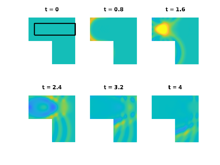
We again set f≡0f\equiv 0, c≡1c\equiv 1, κ≡(1001)\kappa\equiv\begin{pmatrix}1&0\\ 0&1\end{pmatrix} and this time zero initial condition in Ω\Omega, i.e., u0=v0=0u_{0}=v_{0}=0. The scattering problem is excited by 9 sources outside of the domain that focus at a point inside Ω\Omega. Images of the solution in Ω\Omega are shown in Figure 4. No exact solution is available, but further numerical experiments not shown here suggest that the images shown in Figure 4 are accurate.

Refer to caption
Figure 4: Waves focusing at a point in Ω\Omega. In the section of the L-shaped domain indicated by a rectangle in the first image the wave speed is twice as fast as in the remainder of the domain.

References

  • [1] T. Abboud, P. Joly, J. Rodríguez, and I. Terrasse. Coupling discontinuous Galerkin methods and retarded potentials for transient wave propagation on unbounded domains. J. Comput. Phys., 230(15):5877–5907, 2011.
  • [2] A. Bamberger and T. H. Duong. Formulation variationnelle espace-temps pour le calcul par potentiel retardé de la diffraction d’une onde acoustique. I. Math. Methods Appl. Sci., 8(3):405–435, 1986.
  • [3] A. Bamberger and T. H. Duong. Formulation variationnelle pour le calcul de la diffraction d’une onde acoustique par une surface rigide. Math. Methods Appl. Sci., 8(4):598–608, 1986.
  • [4] L. Banjai. Multistep and multistage convolution quadrature for the wave equation: algorithms and experiments. SIAM J. Sci. Comput., 32(5):2964–2994, 2010.
  • [5] L. Banjai. Time-domain Dirichlet-to-Neumann map and its discretization. IMA J. Numer. Anal., 34(3):1136–1155, 2014.
  • [6] L. Banjai and M. Kachanovska. Fast convolution quadrature for the wave equation in three dimensions. J. Comput. Phys., 279:103–126, 2014.
  • [7] L. Banjai, C. Lubich, and F.-J. Sayas. Stable numerical coupling of exterior and interior problems for the wave equation. Numer. Math., 129(4):611–646, 2015.
  • [8] L. Banjai and F.-J. Sayas. Integral equation methods for evolutionary PDE. Springer Series in Computational Mathematics. Springer, To be published in 2022.
  • [9] S. C. Brenner and L. R. Scott. The mathematical theory of finite element methods, volume 15 of Texts in Applied Mathematics. Springer-Verlag, New York, 1994.
  • [10] G. Cohen and S. Pernet. Finite element and discontinuous Galerkin methods for transient wave equations. Scientific Computation. Springer, Dordrecht, 2017. With a foreword by Patrick Joly.
  • [11] M. Costabel and F.-J. Sayas. Time-dependent problems with boundary integral equation method. In Encyclopedia of Computational Mechanics Second Edition. Part 2, pages 1–24. John Wiley & Sons, Ltd., 2017.
  • [12] H. Eruslu and F.-J. Sayas. Polynomially bounded error estimates for trapezoidal rule convolution quadrature. Comput. Math. Appl., 79(6):1634–1643, 2020.
  • [13] L. C. Evans. Partial differential equations, volume 19 of Graduate Studies in Mathematics. American Mathematical Society, Providence, RI, 1998.
  • [14] S. Falletta and G. Monegato. An exact non reflecting boundary condition for 2D time-dependent wave equation problems. Wave Motion, 51(1):168–192, 2014.
  • [15] S. Falletta and G. Monegato. Exact non-reflecting boundary condition for 3D time-dependent multiple scattering–multiple source problems. Wave Motion, 58:281–302, 2015.
  • [16] E. Hairer, C. Lubich, and M. Schlichte. Fast numerical solution of nonlinear Volterra convolution equations. SIAM J. Sci. Statist. Comput., 6(3):532–541, 1985.
  • [17] M. E. Hassell and F.-J. Sayas. A fully discrete BEM-FEM scheme for transient acoustic waves. Comput. Methods Appl. Mech. Engrg., 309:106–130, 2016.
  • [18] C. Johnson and J.-C. Nédélec. On the coupling of boundary integral and finite element methods. Math. Comp., 35(152):1063–1079, 1980.
  • [19] A. R. Laliena and F.-J. Sayas. Theoretical aspects of the application of convolution quadrature to scattering of acoustic waves. Numer. Math., 112(4):637–678, 2009.
  • [20] C. Lubich. Convolution quadrature and discretized operational calculus. II. Numer. Math., 52(4):413–425, 1988.
  • [21] C. Lubich. On the multistep time discretization of linear initial-boundary value problems and their boundary integral equations. Numer. Math., 67:365–389, 1994.
  • [22] D. Pölz and M. Schanz. On the space-time discretization of variational retarded potential boundary integral equations. Comp. Math. Appl., 99:195–210, 2021.
  • [23] NIST Digital Library of Mathematical Functions. http://dlmf.nist.gov/, Release 1.1.1 of 2021-03-15. F. W. J. Olver, A. B. Olde Daalhuis, D. W. Lozier, B. I. Schneider, R. F. Boisvert, C. W. Clark, B. R. Miller, B. V. Saunders, H. S. Cohl, and M. A. McClain, eds.
  • [24] S. A. Sauter and C. Schwab. Boundary Element Methods, volume 39 of Springer Series in Computational Mathematics. Springer-Verlag, Berlin, 2011.
  • [25] F.-J. Sayas. Retarded Potentials and Time Domain Boundary Integral Equations, volume 50 of Springer Series in Computational Mathematics. Springer, [Cham], 2016. A road map.
  • [26] D. Soares, W. Mansur, and O. Von Estorff. An efficient time-domain FEM/BEM coupling approach based on FEM implicit Green’s functions and truncation of BEM time convolution process. Computer Methods in Applied Mechanics and Engineering, 196(9):1816–1826, 2007.