New criterions on nonexistence of periodic orbits of planar dynamical systems and their applications

Hebai Chen¹, Hao Yang¹, Rui Zhang¹, Xiang Zhang² Address: ¹ School of Mathematics and Statistics, HNP-LAMA, Central South University, Changsha, Hunan 410083, P. R. China Address: ² School of Mathematical Sciences, MOE-LSC, Shanghai Jiao Tong University, Shanghai, 200240, P.R. China Email address: chen_hebai@csu.edu.cn (H. Chen), y_ang_hao@163.com (H. Yang), zhang_rui@csu.edu.cn (R. Zhang), xzhang@sjtu.edu.cn (X. Zhang)

Abstract.

Characterizing existence or not of periodic orbit is a classical problem and it has both theoretical importance and many real applications. Here, several new criterions on nonexistence of periodic orbits of the planar dynamical system $\dot{x}=y,~\dot{y}=-g(x)-f(x,y)y$ are obtained in this paper, and by examples showing that these criterions are applicable, but the known ones are invalid to them. Based on these criterions, we further characterize the local topological structures of its equilibrium, which also show that one of the classical results by A.F. Andreev [Amer. Math. Soc. Transl. 8 (1958), 183–207] on local topological classification of the degenerate equilibrium is incomplete. Finally, as another application of these results, we classify the global phase portraits of a planar differential system, which comes from the third question in the list of the 33 questions posed by A. Gasull and also from a mechanical oscillator under suitable restriction to its parameters.

Key words and phrases:

Limit cycle, non–existence, nilpotent equilibrium, Andreev topological classification, global phase portrait.

2010 Mathematics Subject Classification

34C07, 34A05, 34A34, 34C14

1. Introduction

As we all know, Hilbert’s 23 problems were posed by the famous mathematian D. Hilbert at the International Congress of Mathematicians in 1900, see [13], where the second half of Hilbert’s 16th problem is to study the maximum number and their relative position of limit cycles of planar polynomial differential systems. Up to now, Hilbert’s 16th problem is still unsolved. On the other hand, to study dynamics of a planar dynamical system, it is usually very important to characterize existence of its limit cycles.

For the aforementioned reasons, the study of limit cycles of planar dynamical systems has been attracting many famous mathematicians working on it, see for instance Dulac [10], Itenberg and Shustin [15], Lins et al [17], Roussaries [21], Smale [23], Ye [26]and Zhang et al [29], and the references therein. Notice that most of the known results on nonlocal limit cycles are for existence and uniqueness. In order to prove existence of limit cycles, one of the essential tools is the Poincaré-Bendixson annulus theorem. On uniqueness of the limit cycle, most of the results were limited to Liénard systems and generalized Liénard systems, such as Levinson et al [16], Liou and Cheng [18], Wang and Kooij [24], Xiao and Zhang [25], Zeng [27], Zeng et al [28] and Zhang et al [29], and so on. However, for nonexistence of the limit cycle of planar differential equations, the theoretical results are far less than those for existence of limit cycles. At present, Poincaré’s method of tangential curves [29, Theorem 1.6 of Chapter 4] and the Dulac criterion [29, Theorem 1.7 of Chapter 4] are common tools to study nonexistence of limit cycles, but it is not an easy task to find the Poincaré function $F(x,y)$ or Dulac function $B(x,y)$ in applications. Besides, most of the results on nonexistence of limit cycles are focused on Liénard and generalized Liénard systems, which can be found in [4, 5, 9, 22] and their references. See Appendix, where we list some known results for comparing with ours and their applications. Besides, there are also a few theoretical results on nonexistence of limit cycles for general planar differential systems.

The goal of this paper is to provide certain new criterions on nonexistence of limit cycles of the planar differential system

(1)

\left\{\begin{aligned} \dot{x}&=y,\\ \dot{y}&=-g(x)-f(x,y)y,\end{aligned}\right.

where $x\in(\alpha,\beta)$ , $y\in\mathbb{R}$ , $\alpha<0$ , $\beta>0$ . Notice that system (1) has been widely adopted to model real world problems in applied science and engineering, see [1, 3, 20] and the references therein.

The organization of this paper is as follows. In section 2, we state our main results, which are new criterions on nonexistence of periodic orbits of system (1), and characterization on local topological structures of the related system at its equilibrium. Here we complete the local classification of a degenerate equilibrium (nilpotent one), which is a classical result but incomplete as will be shown. It was initially proved by Andreev [2] in 1958, and then stated and proved in [29] and so on. As we have seen, Andreev’s result was also repeatedly stated in many monographs and papers for classifying topological structures of planar differential systems. Section 3 is the proofs of our main results. Section 4 is partly an application of our theoretical results, where we characterize all global topological phase portraits (Theorems 10 and 11) of a system under certain restriction of parameters, which comes from the first half of the third question in the list of the 33 questions posed by Gasull [12] and also from a mechanical oscillator.

2. Main results

In this section, we state our main results of this paper. The first one provides a criterion on nonexistence of periodic orbits.

Theorem 1.

Assume that $g(x)=-g(-x)$ for all $0\leqslant x<\min\{-\alpha,\beta\}$ , and that the following conditions hold:

(i)

$xg(x)>0$ for all $(\alpha,0)\cup(0,\beta)$ ;
(ii)

$g(x)$ is Lipschitzian continuous for $x\in(\alpha,0)\cup(0,\beta)$ , and $f(x,y)$ is Lipschitzian continuous for $(x,y)\in(\alpha,\beta)\times\mathbb{R}$ ;
(iii)

either $f(x,y)\geqslant-f(-x,y)$ or $f(x,y)\leqslant-f(-x,y)$ for all $0\leqslant x<\min\{-\alpha,\beta\}$ and $y\in\mathbb{R}$ ;
(iv)

$f(x,y)\not\equiv-f(-x,y)$ for $x\in(0,\zeta)$ and $y\in\mathbb{R}$ , where $0<\zeta\ll 1$ .

Then, system (1) has no closed orbits in the strip $\alpha<x<\beta$ .

The second one is another criterion on nonexistence of periodic orbits.

Theorem 2.

Assume that the conditions (i), (ii), (iv) and the following one hold:

(iii^′)

either $f(x,y)\geqslant-f(x,-y)$ or $f(x,y)\leqslant-f(x,-y)$ for all $(x,y)\in(\alpha,\beta)\times\mathbb{R}$ .

Then, system (1) has no closed orbits in the strip $\alpha<x<\beta$ .

Remark 1.

When $g(x)=x$ and $f(x,y)=\hat{f}(y)$ , after the change of variables $(x,y,t)\to(y,x,-t)$ , system (1) is transformed to

\left\{\begin{aligned} \dot{x}&=y+\hat{f}(x)x,\\ \dot{y}&=-x,\end{aligned}\right.

which is in the Liénard form. By Theorem 2 one can directly obtain the results in [17, Proposition 1] $($ see Theorem 14 in Appendix A $)$ . In this sense, Theorem 2 is an extended version of [17, Proposition 1].

The next is the third criterion on nonexistence of periodic orbits.

Theorem 3.

Assume that $g(-x)\not\equiv-g(x)$ for $0\leqslant x<\min\{-\alpha,\beta\}$ ,

g(x)=x^{m}h(x),\ {\rm if}\ x\in(-\epsilon,\epsilon),

where $h(0)>0$ , $m=p/q\geqslant 1$ , $p,q$ are odd and $\epsilon>0$ is small. In addition to the conditions (i) and (ii) of Theorem 1, suppose that for all $\hat{x}<0<x$ satisfying

(2)

\int_{\text{0}}^{x}{g(s)}ds=\int_{\text{0}}^{\hat{x}}{g(s)}ds,

the following hold

(v)

either $f(x,y)/g(x)\geqslant f(\hat{x},y)/g(\hat{x})$ or $f(x,y)/g(x)\leqslant f(\hat{x},y)/g(\hat{x})$ for $0\leqslant x<\min\{-\alpha,\beta\}$ and $y\in\mathbb{R}$ ;
(vi)

$f(x,y)/g(x)\not\equiv f(\hat{x},y)/g(\hat{x})$ for $x\in(0,\zeta)$ and $y\in\mathbb{R}$ , where $0<\zeta\ll 1$ .

Then, system (1) has no closed orbits in the strip $\alpha<x<\beta$ .

Remark 2.

In Theorem 3, if $g(x)\equiv-g(-x)$ then $\int_{\text{0}}^{x}{g(s)}ds=\int_{\text{0}}^{\hat{x}}{g(s)}ds$ holds with $\hat{x}=-x$ . Consequently, $f(x,y)/g(x)\geqslant f(\hat{x},y)/g(\hat{x})$ in (v) implies $f(x,y)\geqslant-f(-x,y)$ , which is (iii). In this sense, Theorem 1 is a special case of Theorem 3. Here, stating Theorem 1 separately has two reasons: one is for its easy application, and second is for distributing the technical parts of the proofs. As it is easy to see, system (1) is an extension of the Liénard system

\dot{x}=y,\,\,\dot{y}=-g(x)-f(x)y,

in which $g(x)$ is usually an odd function, like $g(x)=x$ , or $g(x)=x+x^{3}$ , etc, and so Theorem 1 can be conveniently applied to it.

The fouth one is an extension of Theorem 1, which admits existence of other equilibria than the origin.

Theorem 4.

In case $g(x)=-g(-x)$ for all $0\leqslant x<\min\{-\alpha,\beta\}$ , suppose the conditions (ii), (iii), (iv) of Theorem 1 hold. Then, system (1) has no closed orbits surrounding the origin $O$ in the strip $\alpha<x<\beta$ .

In Theorems 1, 2 and 3, system (1) has a unique equilibrium $O$ and has no closed orbits when the corresponding conditions hold. Naturally, we want to further characterize the qualitative properties of $O$ and the phase portrait of system (1). To avoid much degeneracy, suppose that both $g(x)$ and $f(x,y)$ are analytic functions in a small neighborhood $S_{\delta}(O)$ of the origin $O$ , except a few exception.

If the condition (i) of Theorem 1 holds, then $g^{\prime}(0)\geqslant 0$ . Otherwise, if $g^{\prime}(0)<0$ , there exists an $x_{*}>0$ such that $g(x_{*})<g(0)=0$ , which contradicts $xg(x)>0$ for $x\neq 0$ . Set $a:=g^{\prime}(0)$ , $b:=f(0,0)$ . It is easy to check $b\geqslant 0$ for $f(x,y)/g(x)\geqslant f(\hat{x},y)/g(\hat{x})$ , $b\leqslant 0$ for $f(x,y)/g(x)\leqslant f(\hat{x},y)/g(\hat{x})$ , and $a\geqslant 0$ , where $\hat{x}\leqslant 0\leqslant x$ and $\int_{\text{0}}^{x}{g(s)}ds=\int_{\text{0}}^{\hat{x}}{g(s)}ds$ .

In our next result, we characterize local phase portraits of system (1) with $f(x,y)/g(x)\geqslant f(\hat{x},y)/g(\hat{x})$ and $\int_{\text{0}}^{x}{g(s)}ds=\int_{\text{0}}^{\hat{x}}{g(s)}ds$ for $\hat{x}\leqslant 0\leqslant x$ . The case $f(x,y)/g(x)\leqslant f(\hat{x},y)/g(\hat{x})$ and $\int_{\text{0}}^{x}{g(s)}ds=\int_{\text{0}}^{\hat{x}}{g(s)}ds$ for $\hat{x}\leqslant 0\leqslant x$ can be treated via the transformation $(x,\hat{x},y,t)\to(\hat{x},x,y,-t)$ . So without loss of generality, we consider only the case $b\geqslant 0$ .

For our consideration, the region

\mathscr{G}:=\{(a,b)\in\mathbb{R}^{2}:a\geqslant 0,b\geqslant 0\}

will be separated in the six subregions

	$\displaystyle\mathscr{G}_{1}$	$\displaystyle:=\{(a,b)\in\mathscr{G}:a>0,b>0,b^{2}-4a>0\},$
	$\displaystyle\mathscr{G}_{2}$	$\displaystyle:=\{(a,b)\in\mathscr{G}:a>0,b>0,b^{2}-4a<0\},$
	$\displaystyle\mathscr{G}_{3}$	$\displaystyle:=\{(a,b)\in\mathscr{G}:a>0,b>0,b^{2}-4a=0\},$
	$\displaystyle\mathscr{G}_{4}$	$\displaystyle:=\{(a,b)\in\mathscr{G}:a>0,b=0\},$
	$\displaystyle\mathscr{G}_{5}$	$\displaystyle:=\{(a,b)\in\mathscr{G}:a=0,b>0\},$
	$\displaystyle\mathscr{G}_{6}$	$\displaystyle:=\{(a,b)\in\mathscr{G}:a=b=0\}.$

When $a=b=0$ , in $S_{\delta}(O)$ , $g(x)$ and $f(x,y)$ can be written in the forms

(3)

g(x)=a_{k}x^{k}+O(x^{k+1}),\quad f(x,y)=b_{n}x^{n}+O(x^{n+1})+yp(x,y),

where $a_{k}\neq 0$ , $k>1$ , $b_{n}\in\mathbb{R}$ , and $p(x,y)$ is an analytic function in $S_{\delta}(O)$ . By the condition (i) of Theorem 1, we have

\displaystyle x(a_{k}x^{k}+O(x^{k+1}))>0\ \ \ \ \mbox{\rm i.e.}\ \ \ \ a_{k}x^{k+1}+O(x^{k+2})>0,\,\,\,\,\,x\in S_{\delta}(O),

which implies that

(4)

a_{k}>0\quad\mbox{\rm and }\quad k\ \ \mbox{\rm is odd}.

Without loss of generality, we only consider $b_{n}\geqslant 0$ . The case $b_{n}<0$ can be done via the transformation $(x,y,t,b_{n})\to(x,-y,-t,-b_{n})$ . Next we further divide $\mathscr{G}_{6}$ into the three subregions

	$\displaystyle\mathscr{G}_{61}:=$	$\displaystyle\{(a,b)\in\mathscr{G}_{6}:b_{n}=0\}\cup\{(a,b)\in\mathscr{G}_{6}:b_{n}>0,n>(k-1)/2\}$
		$\displaystyle\cup\{(a,b)\in\mathscr{G}_{6}:b_{n}>0,n=(k-1)/2,b_{n}^{2}-2(k+1)a_{k}<0\},$
	$\displaystyle\mathscr{G}_{62}:=$	$\displaystyle\{(a,b)\in\mathscr{G}_{6}:b_{n}>0,n<(k-1)/2,n\text{ even}\}$
		$\displaystyle\cup\{(a,b)\in\mathscr{G}_{6}:b_{n}>0,n=(k-1)/2,b_{n}^{2}-2(k+1)a_{k}\geqslant 0,n\text{ even}\},$
	$\displaystyle\mathscr{G}_{63}:=$	$\displaystyle\{(a,b)\in\mathscr{G}_{6}:b_{n}>0,n<(k-1)/2,n\text{ odd}\}$
		$\displaystyle\cup\{(a,b)\in\mathscr{G}_{6}:b_{n}>0,n=(k-1)/2,b_{n}^{2}-2(k+1)a_{k}\geqslant 0,n~\text{odd}\}.$

Having the above preparation, we can state our next results on global structure of system (1).

Theorem 5.

For system (1), suppose that

•

$\alpha=-\infty$ and $\beta=+\infty$ , $g(x)$ is analytic in $|x|<\epsilon$ $(\epsilon>0$ is small $)$ and $f(x,y)$ is analytic in $S_{\delta}(O)$ ,
•

$xg(x)>0$ for all $x\neq 0$ , $g(x)$ and $f(x,y)$ are Lipschitzian continuous for $(x,y)\in\mathbb{R}^{2}$ ,
•

either $f(x,y)\equiv-f(-x,y)$ for $g(x)=-g(-x)$ in $(x,y)\in(0,+\infty)\times\mathbb{R}$ , or $f(x,y)/g(x)\equiv f(\hat{x},y)/g(\hat{x})$ for $g(x)\not\equiv-g(-x)$ in $(x,y)\in(0,+\infty)\times\mathbb{R}$ , where $\hat{x}<0<x$ satisfying equation (2).

The following statements hold.

•

The origin $O$ of system (1) is a center, or $S_{\delta}(O)$ consists of one elliptic sector and one hyperbolic sector, or $S_{\delta}(O)$ consists of one elliptic sector, one hyperbolic sector and two parabolic sectors. Figure 1 illustrates these local structures at $O$ .

(a) $(a,b)\in\mathscr{G}_{63}$

(b) $(a,b)\in\mathscr{G}_{63}$

(c) $(a,b)\in\mathscr{G}_{63}$

(d) $(a,b)\in\mathscr{G}_{4}\cup\mathscr{G}_{61}$

Figure 1. Phase portraits of system (1) when $f(x,y)/g(x)\equiv f(\hat{x},y)/g(\hat{x})$ . (The elliptic sector is bounded in (a), and unbounded in (b) and (c).)
•

When the elliptic sector is bounded, there has no parabolic sectors at $O$ . In other words, two parabolic sectors appearing in a neighborhood of $O$ happens only in the unbounded case of the elliptic sector. These two situations can be realized by concrete examples.

Theorem 6.

For system (1), suppose that

•

$\alpha=-\infty$ and $\beta=+\infty$ , $g(x)$ is analytic in $|x|<\epsilon$ $(\epsilon>0$ is small $)$ , and $f(x,y)$ is analytic in $S_{\delta}(O)$ ,
•

$xg(x)>0$ for all $x\neq 0$ , $g(x)$ and $f(x,y)$ are Lipschitzian continuous for $(x,y)\in\mathbb{R}^{2}$ ,
•

either $f(x,y)\geqslant-f(-x,y)$ for $g(x)=-g(-x)$ in $(x,y)\in(0,+\infty)\times\mathbb{R}$ , or $f(x,y)/g(x)\geqslant f(\hat{x},y)/g(\hat{x})$ for $g(x)\not\equiv-g(-x)$ in $(x,y)\in(0,+\infty)\times\mathbb{R}$ , where $\hat{x}<0<x$ satisfying equation (2),
•

$f(x,y)\not\equiv-f(-x,y)$ as $g(x)=-g(-x)$ for $(x,y)\in(0,\zeta)\times\mathbb{R}$ and $f(x,y)/g(x)\not\equiv f(\hat{x},y)/g(\hat{x})$ as $g(x)\not\equiv-g(-x)$ for $(x,y)\in(0,\zeta)\times\mathbb{R}$ , where $0<\zeta\ll 1$ .

Then, the qualitative property of the unique equilibrium $O$ is as that shown in Table 1 and system (1) could have only possibly seven local phase portraits, as those shown in Figures 1(b) and (c) and Figure 2.

Table 1. The qualitative property of

O

of system (1).

(a,b)

Type of

O

Geometric configurations

\mathscr{G}_{1}\cup\mathscr{G}_{5}

stable node

S_{\delta}(O)

except one pair of orbits approaching

O

in one of the directions

\theta_{2}

and

\theta_{4}

all other orbits approaching

O

in one of

the directions

\theta_{1}

and

\theta_{3}

, see Figure 2(a).

\mathscr{G}_{2}\cup\mathscr{G}_{4}\cup\mathscr{G}_{61}

stable focus

S_{\delta}(O)

all orbits rotate clockwise, see Figure 2(b).

\mathscr{G}_{3}\cup\mathscr{G}_{62}

stable

improper node

S_{\delta}(O)

all orbits approaching

O

along one of the directions

\theta_{5}

and

\theta_{6}

, see Figure 2(c).

\mathscr{G}_{63}

a degenerate one

elliptic sector

is bounded

S_{\delta}(O)

consist of one elliptic sector,

one hyperbolic sector and

one parabolic sector, see Figure 2(d).

elliptic sector is unbounded

S_{\delta}(O)

consist of one elliptic sector,

one hyperbolic sector and

zero parabolic sector, see Figure 1(c).

S_{\delta}(O)

consist of one elliptic sector,

one hyperbolic sector and

one parabolic sector, see Figure 2(e).

S_{\delta}(O)

consist of one elliptic sector,

one hyperbolic sector and

two parabolic sectors, see Figure 1(b).

Remark : $\theta_{1}=\pi-\arctan\left(b-\sqrt{b^{2}-4a})/2\right),\theta_{2}=\pi-\arctan\left(b+\sqrt{b^{2}-4a})/2\right),\theta_{3}=2\pi-\arctan\left(b-\sqrt{b^{2}-4a})/2\right),\theta_{4}=2\pi-\arctan\left(b+\sqrt{b^{2}-4a})/2\right),\theta_{5}=\pi-\arctan\left(b/2\right),\theta_{6}=2\pi-\arctan\left(b/2\right)$ .

Refer to caption — (a) $(a,b)\in\mathscr{G}_{1}\cup\mathscr{G}_{5}$

Remark 3.

For system (38) in Appendix B, Andreev [2] proved that when $b_{n}\neq 0$ and $n<(k-1)/2$ , or $b_{n}\neq 0$ , $n=(k-1)/2$ and $b_{n}^{2}-2(k+1)a_{k}\geqslant 0$ with $n$ and $k$ odd, any small neighborhood $S_{\delta}(O)$ of system (38) at $O$ consists of only one elliptic sector and one hyperbolic sector. This result has also been collected in many Monographs and papers for their applications on local classification of equilibria, see for instance [29, Theorem 7.2 of Chapter 2], [8, Theorem 3.5 of Chapter 3] and so on. However, as we show, this classification is incomplete. In fact, beside the elliptic and hyperbolic sectors, there may include zero $($ see system (23) with Figure 7 $)$ , or one $($ see Example 2 with Figure 4 $)$ , or two parabolic sectors $($ see Example 1 with Figure 3 $)$ in $S_{\delta}(O)$ . Andreev [2] proved the existence of the elliptic sector without discussing its boundedness. In fact, our results indicate that even in the bounded case, the existence of a parabolic sector strongly depends on symmetry of the vector field with respect to some line passing the equilibrium $($ no parabolic sector in symmetric case, and a unique one in nonsymmetric case $)$ .

Remark 4.

If the elliptic sector is bounded and the vector field is not symmetry, $S_{\delta}(O)$ includes exactly one parabolic sector. However, when the elliptic sector is unbounded, we have only proved that $S_{\delta}(O)$ contains at most two parabolic sectors, and provide examples which do have two parabolic sectors. But we cannot find examples with zero or one parabolic sector in $S_{\delta}(O)$ , and also cannot prove that $S_{\delta}(O)$ must have exactly two parabolic sectors. This will remain for further study.

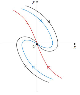
When $(a,b)\in\mathscr{G}_{63}$ , the next two examples illustrate existence of two parabolic sectors together with one unbounded elliptic and one hyperbolic sectors, and also of one parabolic sector together with one bounded elliptic and one hyperbolic sectors in a neighborhood of a nilpotent equilibrium.

Example 1.

The planar differential system

(5)

\displaystyle\dot{x}=y,\quad\dot{y}=-2x^{3}-4xy+\varepsilon\widetilde{g}(r)x^{2}y,

with $\varepsilon\geqslant 0$ sufficiently small, $r^{2}=x^{2}+y^{2}$ , and

\widetilde{g}(r)=\left\{\begin{aligned} &1,~&&{\rm if}~0\leqslant r\leqslant 1,\\ &0,~&&{\rm if}~r\geqslant 2,\end{aligned}\right.

decreasing and smooth for $r\geqslant 0$ , has the global phase portrait as that shown in Figure 3.

Notice that system (5) satisfies all conditions of Theorem 6 and $(a,b)\in\mathscr{G}_{63}$ . The proof of the conclusion in this example will be included in the proof of Theorem 6.

Example 2.

Beside the elliptic sector $($ bounded by assumption $)$ and hyperbolic sector system (1) has only one parabolic sector in $S_{\delta}(O)$ . Figure 4 illustrates this asymmetric case with one parabolic sector for system $\dot{x}=y,\ \dot{y}=-2x^{5}+x^{6}-xy$ in a neighborhood of the origin by Matlab with the initial points $(0,0.31),\ (0,0.11),\ (0,-0.3)$ .

As shown in Table 1 of Theorem 6, the qualitative property of $O$ is related to the boundedness of the elliptic sector when $(a,b)\in\mathscr{G}_{63}$ . The following proposition provides a criterion on existence of the bounded elliptic sector (if exists) for the Liénard differential system (1) with $f(x,y)$ in $x$ only. Taking $f(x,y)=\widetilde{f}(x)$ , with the transformation $(x,y)\to(x,y-F(x))$ , system (1) can be written in the classical Liénard system

(6)

\dot{x}=y-F(x),\,\,\dot{y}=-g(x),

where $F^{\prime}(x)=\widetilde{f}(x)$ .

Proposition 7.

For system (6), suppose that

•

$xg(x)>0$ for all $x\neq 0$ , and $\int_{0}^{\infty}g(x)dx=+\infty$ ,
•

$g(x)$ and $F(x)$ are Lipschitzian continuous in $\mathbb{R}$ , and are analytic in $|x|<\epsilon$ for some small $\epsilon>0$ is small,
•

system (6) has an elliptic sector at $O$ , i.e. $(a,b)\in\mathscr{G}_{63}$ .

If there exists an $x_{0}\neq 0$ such that $F(x_{0})=0$ , the elliptic sector is bounded.

Notice that Ding [7] proved the boundedness of the maximal elliptic sector of the following Liénard system

(7)

\displaystyle\dot{x}=y+\frac{1}{2}x^{2}-\frac{1}{3}x^{3},\ \dot{y}=-kx^{3},

for $k\in(0,1/8)$ . Applying Proposition 7, one can conclude that the elliptic sector of system (7) at the origin is bounded for all $k>0$ . This generalizes the result of Ding [7].

3. Proofs of main results

This section is the proofs of our main results.

3.1. Proof of Theorem 1

We consider only the case $f(x,y)\geqslant-f(-x,y)$ for $x\geqslant 0$ of the condition (iii), since the case $f(x,y)\leqslant-f(-x,y)$ for $x\geqslant 0$ can be transformed to the former by $(x,y,t)\to(-x,y,-t)$ . With the transformation $(x,y)\to(-x,y)$ , system (1) is changed into

(8)

\left\{\begin{aligned} \dot{x}&=-y,\\ \dot{y}&=g(x)-f(-x,y)y.\end{aligned}\right.

It is clear that systems (1) and (8) can be rewritten as

(9)

\frac{dy}{dx}=-\frac{g(x)}{y}-f(x,y),

and

(10)

\frac{dy}{dx}=-\frac{g(x)}{y}+f(-x,y),

respectively.

Assume by contrary that system (1) has a closed orbit $\Gamma$ in the strip $\alpha<x<\beta$ . It is obvious that $\Gamma$ must intersect the negative and positive $y$ –axes, saying at $A$ and $B$ , respectively, and the positive $x$ –axis, saying at $C$ . Observe that the orbit arc, denoted by $\widehat{AB}$ , of $\Gamma$ in $x\geqslant 0$ satisfies equation (9). Because of $\dot{x}=y$ there, the orbit arc $\widehat{AC}$ can be represented as $y=y_{1}(x)$ . Consider the orbit arc $\widehat{AD}$ of equation (10) starting from $A$ and ending at $D$ a point on the positive $x$ –axis, and represent it by $y=y_{2}(x)$ . See Figure 5.

Let $\varphi(x)=y_{2}(x)-y_{1}(x)$ . Direct calculations show that

(11)	$\displaystyle\varphi(x)$	$\displaystyle=y_{2}(x)-y_{1}(x)$
		$\displaystyle=\left.(y_{2}(s)-y_{1}(s))\right\|^{x}_{0}$
		$\displaystyle=\int_{0}^{x}\left(-\frac{g(s)}{y_{2}(s)}+f(-s,y_{2}(s))\right)ds-\int_{0}^{x}\left(-\frac{g(s)}{y_{1}(s)}-f(s,y_{1}(s))\right)ds$
		$\displaystyle=\int_{0}^{x}\left(g(s)\frac{y_{2}(s)-y_{1}(s)}{y_{2}(s)y_{1}(s)}\right)ds+\int_{0}^{x}\left(f(s,y_{1}(s))+f(-s,y_{2}(s))\right)ds$
		$\displaystyle=\int_{0}^{x}\left(g(s)\frac{y_{2}(s)-y_{1}(s)}{y_{2}(s)y_{1}(s)}+f(s,y_{1}(s))-f(s,y_{2}(s))\right)ds$
		$\displaystyle+\int_{0}^{x}\left(f(s,y_{2}(s))+f(-s,y_{2}(s))\right)ds$
		$\displaystyle=\int_{0}^{x}M(s)\left(y_{2}(s)-y_{1}(s)\right)ds+N(x),$

where

M(x)=\left\{\begin{aligned} &\frac{g(x)}{y_{2}(x)y_{1}(x)}-\frac{f(x,y_{2}(x))-f(x,y_{1}(x))}{y_{2}(x)-y_{1}(x)},\,\,\,&{\rm if}\,y_{1}(x)\neq y_{2}(x),\\ &\frac{g(x)}{y_{2}(x)y_{1}(x)},\,\,\,&{\rm if}\,y_{1}(x)=y_{2}(x),\end{aligned}\right.

and

N(x)=\int_{0}^{x}f(s,y_{2}(s))+f(-s,y_{2}(s))ds.

By (11), it follows that

(12)

\displaystyle\varphi(x)=\int_{0}^{x}M(s)\varphi(s)ds+N(x).

Letting $H(x)=\int_{0}^{x}M(s)\varphi(s)ds$ , we obtain

(13)

\displaystyle\frac{dH(x)}{dx}=M(x)\varphi(x)=M(x)H(x)+M(x)N(x).

Using variation of constants formula to solve (13) yields

(14)		$\displaystyle H(x)$	$\displaystyle=\exp\left(\int_{0}^{x}M(s)ds\right)\cdot\int_{0}^{x}\left[M(s)N(s)\exp\left(-\int_{0}^{s}M(\xi)d\xi\right)\right]ds$
(14)			$\displaystyle=\int_{0}^{x}M(s)N(s)\exp\left(\int_{s}^{x}M(\xi)d\xi\right)ds.$

Combining the formulas (12) through (14), one has

	$\displaystyle\varphi(x)$	$\displaystyle=H(x)+N(x)$
		$\displaystyle=\int_{0}^{x}M(s)N(s)\exp\left(\int_{s}^{x}M(\xi)d\xi\right)ds+N(x)$
		$\displaystyle=N(0)\exp\left(\int_{0}^{x}M(s)ds\right)+\int_{0}^{x}N^{\prime}(s)\exp\left(\int_{s}^{x}M(\xi)d\xi\right)ds$
		$\displaystyle=\int_{0}^{x}N^{\prime}(s)\exp\left(\int_{s}^{x}M(\xi)d\xi\right)ds$
		$\displaystyle=\int_{0}^{x}\left(f(s,y_{2}(s))+f(-s,y_{2}(s))\right)\exp\left(\int_{s}^{x}M(\xi)d\xi\right)ds.$

By the conditions $f(x,y)\geqslant-f(-x,y)$ for $0<x<\min\{-\alpha,\beta\}$ , $y\in\mathbb{R}$ , and $f(x,y)\not\equiv-f(-x,y)$ for $x\in(-\zeta,\zeta)$ , $y\in\mathbb{R}$ , $\forall~\zeta>0$ , it follows that

\displaystyle\varphi(x)=\int_{0}^{x}\left(f(s,y_{2}(s))+f(-s,y_{2}(s))\right)\exp\left(\int_{s}^{x}M(\xi)d\xi\right)ds>0.

Consequently, $y_{2}(x)>y_{1}(x)$ . That is, the point $D$ must be located on the left hand–side of the point $C$ . Similar arguments verify that the orbit arc $\widehat{BE}$ of equation (10) starting from $B$ and ending at $E$ on the positive $x$ –axis will have $E$ being on the right hand-side of $C$ . This implies that system (10) does not have an orbit arc linking the points $A$ and $B$ , and so has no a closed orbit in the strip $\alpha<x<\beta$ .

It completes the proof of Theorem 1. $\hfill\square$

Remark 5.

In the proof of Theorem 1, we cannot apply directly the comparison theorem $($ see [14, Theorem 6.1 of Chapter 1] $)$ to obtain $\varphi(x)>0$ , since we only obtain $\varphi(x)\geqslant 0$ by that theorem. That is the reason why we need a more accurate estimate.

3.2. Proof of Theorem 2

We consider only the case $f(x,y)\geqslant-f(x,-y)$ for $y\geqslant 0$ of the condition (iii^′), since the case $f(x,y)\leqslant-f(x,-y)$ for $x\geqslant 0$ can be transformed to the former by $(x,y,t)\to(x,-y,-t)$ . With the transformation $(x,y)\to(x,-y)$ , system (1) is changed into

(15)

\left\{\begin{aligned} \dot{x}&=-y,\\ \dot{y}&=g(x)-f(x,-y)y.\end{aligned}\right.

It is clear that systems (1) and (15) can be rewritten as (9) and

(16)

\frac{dy}{dx}=-\frac{g(x)}{y}+f(x,-y),

respectively.

Assume by contrary that system (1) has a closed orbit $\Gamma$ in the strip $\alpha<x<\beta$ . It is obvious that $\Gamma$ must intersect the negative and positive $x$ –axes, saying at $A$ and $B$ , respectively, and the positive $y$ –axis, saying at $C$ . Observe that the orbit arc, denoted by $\widehat{AB}$ , of $\Gamma$ in $y\geqslant 0$ satisfies equation (9). Because of $\dot{x}=y$ there, the orbit arc $\widehat{AC}$ can be represented as $y=y_{1}(x)$ . Consider the orbit arc $\widehat{AE}$ of equation (16) starting from $A$ and ending at $E$ a point on the positive $y$ –axis, and represent it by $y=y_{2}(x)$ . See Figure 6.

Let $\varphi(x)=y_{2}(x)-y_{1}(x)$ . Then, we can show $\varphi(0)>0$ . The remainder of the proof of this result is quiet similar to that given earlier for Theorem 1 and so is omitted.

3.3. Proof of Theorem 3

With the transformation

(17)

u=\left({(m+1)G(x)}\right)^{\frac{1}{m+1}}\text{sgn}(x),\quad d\tau=\frac{g(x)}{u^{m}}dt,

system (1) is changed to

(18)

\left\{\begin{aligned} \frac{du}{d\tau}&=y,\\ \frac{dy}{d\tau}&=-u^{m}-\frac{f(x(u),y)}{g(x(u))}u^{m}y=:-u^{m}-F(u,y)y,\end{aligned}\right.

where $G(x)=\int_{0}^{x}g(s)ds$ . By (17) and $xg(x)>0$ for $x\in(\alpha,0)\cup(0,\beta)$ , it follows that $u=\left({(m+1)G(x)}\right)^{1/(m+1)}\text{sgn}(x)$ has the inverse function $x=x(u)$ and $x(0)=0$ . Moreover, $x=x(u)$ is increasing.

It is easy to obtain that

\lim_{u\to 0}\frac{u^{m}}{g(x(u))}=\frac{1}{\sqrt[m+1]{h(0)}}.

One can check that $F(u,y)$ is Lipschitzian continuous for $u\in\left(u(\alpha),u(\beta)\right)$ and $y\in\mathbb{R}$ , i.e., the condition (ii) of Theorem 1 holds. Furthermore,

\frac{f(x,y)}{g(x)}\geqslant(\text{resp.}\leqslant)\frac{f(\hat{x},y)}{g(\hat{x})}

implies

F(u,y)\geqslant(\text{resp.}\leqslant)-F(-u,y),

where $\hat{x}\leqslant 0\leqslant x$ satisfies $\int_{\text{0}}^{x}{g(s)}ds=\int_{\text{0}}^{\hat{x}}{g(s)}ds$ . That is, the condition (iii) of Theorem 1 holds. Moreover, it is easy to check that the conditions (i) and (iv) of Theorem 1 hold, too. By Theorem 1, system (18) has no a closed orbit surrounding the origin. $\hfill\square$

3.4. Proof of Theorem 4

As proved in Theorem 1, by contrary assume that system (1) has a closed orbit $\Gamma^{\prime}$ surrounding the origin in the strip $\alpha<x<\beta$ . Let $A^{\prime}$ be the intersection point of $\Gamma^{\prime}$ with the negative $y$ –axis, and let $\widehat{A^{\prime}C^{\prime}}$ and $\widehat{A^{\prime}D^{\prime}}$ , represented by $y=y_{3}(x)$ and $y=y_{4}(x)$ , be the orbit arcs of systems (9) and (10) starting from $A^{\prime}$ and ending at respectively $C^{\prime}$ and $D^{\prime}$ , which are points on the $x$ –axis. Set $\varphi_{1}(x)=y_{4}(x)-y_{3}(x)$ . By a similar calculation as that in the proof of Theorem 1, we can obtain that

(19)

\displaystyle\varphi_{1}(x)=\int_{0}^{x}\left(f(s,y_{4}(s))+f(-s,y_{4}(s))\right)\exp\left(\int_{s}^{x}M_{1}(\xi)d\xi\right)ds,

where

M_{1}(x)=\left\{\begin{aligned} &\frac{g(x)}{y_{3}(x)y_{4}(x)}-\frac{f(x,y_{4}(x))-f(x,y_{3}(x))}{y_{4}(x)-y_{3}(x)},\,\,\,{\rm if}\,y_{3}(x)\neq y_{4}(x),\\ &\frac{g(x)}{y_{3}(x)y_{4}(x)},\,\,\,\qquad\qquad\qquad\qquad\qquad\qquad{\rm if}\,y_{3}(x)=y_{4}(x).\end{aligned}\right.

Our main goal is to obtain the sign of $\varphi_{1}(x)$ . Since $\exp\left(\int_{s}^{x}M_{1}(\xi)d\xi\right)>0$ , the sign of $\varphi_{1}(x)$ in (19) is only associated with $f(x,y)+f(-x,y)$ . Thus, $\varphi_{1}(x)>(\text{resp.}<)\ 0$ when $f(x,y)\geqslant(\text{resp.}\leqslant)-f(-x,y)$ with the equality not identically satisfied. Hence, system (1) has no a closed orbit surrounding the origin $O$ . $\hfill\square$

We remark that Theorem 4 ensures that system (1) has no a closed orbit surrounding the origin $O$ , but does not provide any information on existence of closed orbits around other equilibria in the strip $\alpha<x<\beta$ . The next example is an illustration on nonexistence of closed orbit around the origin and existence of closed orbit around other equilibrium.

Example 3.

Consider the system

(20)

\left\{\begin{aligned} \frac{dx}{dt}&=y,\\ \frac{dy}{dt}&=-g(x)+\mu_{1}y+\mu_{2}xy+x^{2}y,\end{aligned}\right.

where

g(x)=\left\{\begin{aligned} &x-1,~&&{\rm if}~x\geqslant\frac{1}{2},\\ &-3x+1,~&&{\rm if}~\frac{1}{4}<x<\frac{1}{2},\\ &x,~&&{\rm if}~-\frac{1}{4}\leqslant x\leqslant\frac{1}{4},\\ &-3x-1,~&&{\rm if}~-\frac{1}{2}<x<-\frac{1}{4},\\ &x+1,~&&{\rm if}~x\leqslant-\frac{1}{2},\end{aligned}\right.

with $x,y\in\mathbb{R}$ , $\mu_{1},\mu_{2}$ being parameters such that $-\mu_{1}-\mu_{2}-1>0$ sufficiently small and $\mu_{1}\geqslant 0$ .

We claim that system (20) has no a closed orbit around $O$ , but has one surrounding $(1,0)$ for $-\mu_{1}-\mu_{2}-1>0$ sufficiently small and $\mu_{1}\geqslant 0$ . Indeed, one can check that system (20) satisfies (ii)–(iv) of Theorem 1. The first argument of the claim follows from Theorem 4.

To prove the second argument of the claim, we restrict to a small neighborhood of the equilibrium $(x,y)=(1,0)$ , then system (20) is of form

(21)

\left\{\begin{aligned} \frac{dx}{dt}&=y,\\ \frac{dy}{dt}&=1-x+\mu_{1}y+\mu_{2}xy+x^{2}y.\end{aligned}\right.

After the transformation $(x,y)\to(x+1,y)$ , system (21) is changed to

(22)

\left\{\begin{aligned} \frac{dx}{dt}&=y,\\ \frac{dy}{dt}&=-x+(\mu_{1}+\mu_{2}+1)y+(\mu_{2}+2)xy+x^{2}y.\end{aligned}\right.

When $\mu_{1}+\mu_{2}+1=0$ , it is easy to check that $(0,0)$ of (22) is an unstable weak focus of order one, see [6, p.203 ]. Thus, by Hopf bifurcation an unstable limit cycle births from the origin of system (22) when $-\mu_{1}-\mu_{2}-1>0$ is sufficiently small. The proof is done.

3.5. Proof of Theorem 5

We only consider the case $g(x)=-g(-x)$ for $x>0$ since the other case $g(x)\not\equiv-g(-x)$ for $x>0$ can be studied in the same way. In fact, the transformation (17) can sends system (1) in an equivalent way to system (18), which has the new $g(u)$ an odd function.

The condition $f(x,y)\equiv-f(-x,y)$ implies $b=0$ . Furthermore, the assumptions $g(x)=-g(-x)$ and $f(x,y)\equiv-f(-x,y)$ in $(x,y)\in(0,+\infty)\times\mathbb{R}$ mean that the vector field associated to system (1) is symmetric with respect to the $y$ –axis.

If $a=g^{\prime}(0)>0$ , i.e., $(a,b)\in\mathscr{G}_{4}$ , by Lemma 8, $O$ is a center or focus of system (1). The symmetry of the vector field forces that $O$ must be a center, see Figure 1(c).

If $a=0$ , i.e., $(a,b)\in\mathscr{G}_{6}$ , Lemma 8 and its proof verify that $O$ is a nilpotent equilibrium. Again the condition $f(x,y)\equiv-f(-x,y)$ can be written as

-b_{n}x^{n}-O(x^{n+1})-yp(x,y)-b_{n}(-x)^{n}-O((-x)^{n+1})-yp(-x,y)\equiv 0,

which means that $n$ is odd. Consequently, $\mathscr{G}_{6}=\mathscr{G}_{61}\cup\mathscr{G}_{63}$ .

When $(a,b)\in\mathscr{G}_{61}$ , by Theorem 20 of Appendix B and symmetry of the vector field it follows that $O$ is a nilpotent center, see Figure 1(c).

When $(a,b)\in\mathscr{G}_{63}$ , it follows from Lemmas 7.3 and 7.4 of [29, Chapter 2] that system (1) has infinitely many orbits approaching $O$ along the negative $x$ –axis as $t\to-\infty$ , and also infinitely many orbits approaching $O$ along the positive $x$ –axis as $t\to+\infty$ but has no orbits approaching $O$ along other directions. Next we prove the existence of one elliptic and one hyperbolic sectors under the assumptions of the theorem. As a first step, we consider $g(x)$ and $f(x,y)$ having only the leading terms.

Taking $g(x)=a_{k}x^{k}$ and $f(x,y)=b_{n}x^{n}$ , with $k$ and $n$ odd, such that the assumptions of the theorem hold. Let

H(x,y):=\frac{a_{k}}{k+1}x^{k+1}+\frac{y^{2}}{2},

implying that

\left.\frac{dH(x,y)}{dt}\right|_{\eqref{1}}=-b_{n}x^{n}y^{2}<0

in the first and fourth quadrants of the $(x,y)$ –plane. Therefore, by symmetry of the vector field with respect to the $y$ –axis one can conclude that the positive semi–orbit with an initial point $(0,y_{0})$ lies in the interior enclosed by the closed curve $H(x,y)={y_{0}}^{2}/2$ except the initial point, where $y_{0}>0$ is small. Let $(0,y_{1})$ be the first intersection point of the semi–orbit with the $y$ –axis. Then, $-y_{0}<y_{1}\leqslant 0$ . Again by the symmetry of the vector field, the orbit passing $(0,y_{0})$ is a closed one if $y_{1}<0$ , and is a homoclinic one if $y_{1}=0$ . In conclusion, $S_{\delta}(O)$ includes at least one elliptic sector and one hyperbolic sector.

Next we turn to the general $g(x)=a_{k}x^{k}+O(x^{k+1})$ and $f(x,y)=b_{n}x^{n}+O(x^{n+1})+yp(x,y)$ , which satisfy the assumptions of the theorem. By symmetry of the vector field and the continuous dependence of solutions with respect to initial values and parameters, it follows that $S_{\delta}(O)$ still includes at least one elliptic sector and one hyperbolic sector, see Figures 1(a)–(c).

Finally we study the number of parabolic sectors at $O$ . By symmetry of the vector field with respect to the $y$ –axis, it follows clearly that the number of parabolic sectors at $O$ is even. If all orbits with their $\alpha$ –limit set at $O$ have also their $\omega$ –limit sets $O$ , then $S_{\delta}(O)$ consists of exactly one elliptic and one hyperbolic sectors, see Figure 1(a). If some orbits with their $\alpha$ (resp. $\omega$ )–limit set at $O$ have their $\omega$ (resp. $\alpha$ )–limit sets not at $O$ , then $S_{\delta}(O)$ includes at least two parabolic sectors. The previous proofs have shown that $\theta=0$ and $\theta=\pi$ are the only two exceptional directions, and that the orbits approaching $O$ along $\theta=0$ are in positive sense and along $\theta=\pi$ are in negative sense. These imply that there do not have other hyperbolic sections in $S_{\delta}(O)$ . Consequently, there are exactly two parabolic sectors in $S_{\delta}(O)$ , one repelling and the other attracting. We claim that if the elliptic sector is bounded, then system (1) cannot have parabolic sectors in a neighborhood of $O$ . Indeed, by contrary we assume that system (1) has two parabolic sectors at $O$ . Let $\gamma^{*}$ be the maximal homoclinic orbit to $O$ inside the elliptic sector. By existence of the two parabolic sectors and continuity of solutions with respect to initial values, it follows that there exist orbits inside each of the parabolic sectors which intersect the positive $y$ –axis and are outside $\gamma$ . By symmetry of the vector fields associated to system (1), such kinds of orbits inside the parabolic sectors must be homoclinic to $O$ , and so belong to the elliptic sector. This is in contradiction with the assumption that $\gamma^{*}$ is the maximal homoclinic orbit. The claim follows.

In summary, the above arguments verify the next facts for system (1) at $O$ . If the elliptic sector is bounded, $S_{\delta}(O)$ is composed of exactly one elliptic and one hyperbolic sectors provided that the elliptic sector is bounded. Figure 7 illustrates this case for system

(23)

\dot{x}=y,\ \dot{y}=-2x^{5}-xy,

by Matlab with the initial points $(0,-0.3)$ , $(0,-0.2)$ , $(0,-0.1)$ , $(0,0.1)$ , $(0,0.21)$ , $(0,0.41)$ .

If the elliptic sector is unbounded, $S_{\delta}(O)$ consists of either exactly one elliptic and one hyperbolic sectors (see Figure 1(c)), or one elliptic, one hyperbolic and two parabolic sectors (see Figure 1(b)). Example 1 with $\varepsilon=0$ is in this symmetric case and it has two parabolic sectors in a neighborhood of $O$ , and an unbounded elliptic and a hyperbolic sectors. At the moment we do not have an example without parabolic sectors, and also cannot prove its nonexistence.

3.6. Proof of Theorem 6

To prove this theorem, we first analyse the equilibrium at the origin of system (1).

Lemma 8.

Suppose that all conditions of Theorem 6 hold. The unique equilibrium $O=(0,0)$ has the following qualitative properties.

(F1)

$O$ is a stable node for $(a,b)\in\mathscr{G}_{1}\cup\mathscr{G}_{3}$ , and is a stable focus for $(a,b)\in\mathscr{G}_{2}$ ;
(F2)

$O$ is a center or focus for $(a,b)\in\mathscr{G}_{4}$ ;
(F3)

$O$ is a stable node for $(a,b)\in\mathscr{G}_{5}$ ;
(F4)

$O$ is a degenerate equilibrium for $(a,b)\in\mathscr{G}_{6}$ .

Proof.

It is easy to check that system (1) has the unique equilibrium $O=(0,0)$ , at which the Jacobian matrix of system (1) is

\begin{aligned} \left.J:=\begin{pmatrix}0&1\\ -g^{\prime}(0)-{{f}_{x}}(x,y)y&-{{f}_{y}}(x,y)y-f(x,y)\end{pmatrix}\right|_{(0,0)}=\begin{pmatrix}0&1\\ -a&-b\end{pmatrix}\end{aligned}.

The eigenvalues of $J$ are

\lambda_{1,2}=\frac{-b\pm\sqrt{b^{2}-4a}}{2}.

Obviously, the equilibrium $O$ is a stable node when $(a,b)\in\mathscr{G}_{1}\cup\mathscr{G}_{3}$ , and is a stable focus when $(a,b)\in\mathscr{G}_{2}$ . For $(a,b)\in\mathscr{G}_{4}$ , $\lambda_{1,2}$ is a pair of pure imaginary numbers, and so $O$ is a center or focus. For $(a,b)\in\mathscr{G}_{5}$ , one of $\lambda_{1,2}$ is zero, and the other is nonzero. In $S_{\delta}(O)$ , $g(x)$ and $f(x,y)$ can be rewritten as

g(x)=a_{k}x^{k}+O(x^{k+1}),\quad f(x,y)=b+\hat{f}(x,y),

where $a_{k}>0$ , $k$ is odd, $b>0$ and $\hat{f}(0,0)=0$ . With the transformation $(x,y)\to\left((x-y)/b,y\right)$ , system (1) is changed into

(24)

\dot{x}=by-g\left(\frac{x-y}{b}\right)-f\left(\frac{x-y}{b},y\right)y,\quad\dot{y}=-g\left(\frac{x-y}{b}\right)-f\left(\frac{x-y}{b},y\right)y.

By the implicit function theorem,

-g\left(\frac{x-y}{b}\right)-f\left(\frac{x-y}{b},y\right)y=0

has a unique root $y=\phi(x)=-a_{k}/b^{k+1}x^{k}+o(x^{k})$ for small $|x|>0$ . Thus, in system (24)

\dot{x}|_{y=\phi(x)}=b\phi(x)=-\frac{a_{k}}{b^{k}}x^{k}+o(x^{k}).

By Theorem 19 of Appendix B, the equilibrium $O$ is a stable node. Moreover, by calculation, the origin of system (1) has four exceptional directions

\theta_{1}:=\pi-\arctan\left(\frac{b-\sqrt{b^{2}-4a}}{2}\right),\,\,\,\theta_{2}:=\pi-\arctan\left(\frac{b+\sqrt{b^{2}-4a}}{2}\right),

\theta_{3}:=2\pi-\arctan\left(\frac{b-\sqrt{b^{2}-4a}}{2}\right),\,\,\,\theta_{4}:=2\pi-\arctan\left(\frac{b+\sqrt{b^{2}-4a}}{2}\right)

when $(a,b)\in\mathscr{G}_{1}\cup\mathscr{G}_{5}$ , or has two exceptional directions $\theta_{5}:=\pi-\arctan\left(b/2\right)$ , $\theta_{6}:=2\pi-\arctan\left(b/2\right)$ when $(a,b)\in\mathscr{G}_{3}$ . In the former the origin is a normal node, and in the latter the origin is an improper node.

When $(a,b)\in\mathscr{G}_{6}$ , $\lambda_{1}=\lambda_{2}=0$ , and the linearization of system (1) at $O$ has its coefficient matrix being nilpotent. This means that $O$ is a nilpotent equilibrium. The proof is finished. ∎

Now we are back to the proof of Theorem 6 and focus on the case $g(x)=-g(-x)$ for $x>0$ . The case $g(x)\not\equiv-g(-x)$ for $x>0$ can be handled by applying transformation (17), and so is omitted. Since all conditions of Theorem 1 hold, system (1) has no a closed orbit around the origin.

If $b>0$ (i.e. $(a,b)\in\mathscr{G}_{1}\cup\mathscr{G}_{2}\cup\mathscr{G}_{3}\cup\mathscr{G}_{5}$ ) , by Lemma 8, it is easy to get the local phase portraits of system (1) at $O$ , as those in Figures 2(a)–(c).

For $b=0$ , to classify the local phase portraits of system (1) at $O$ we distinguish two cases: $a>0$ and $a=0$ .

Case 1. $a>0$ (i.e. $(a,b)\in\mathscr{G}_{4}$ ). Since $O$ is a center or a weak focus by (F2) of Lemma 8, and there is no a closed orbit around it, the equilibrium $O$ must be a weak focus of system (1).

To characterize the stability of $O$ , let $M$ be a point on the positive $y$ –axis in $S_{\delta}(O)$ , see Figure 8(a), and let $\varphi(M,I^{+})$ be the positive orbit of system (1) having the initial point $M$ . Obviously $\varphi(M,I^{+})$ has to intersect the negative $y$ –axis at a first time at a point $P$ , and then return to the positive $y$ –axis again at a first time at a point $N$ . Comparing both the positive orbit arc and the negative one starting from $N$ of system (1) in the $x\geqslant 0$ half plane,

one gets from $f(x,y)\geqslant-f(-x,y)$ that

\left.\frac{dy}{dx}\right|_{\eqref{3}}\leqslant\left.\frac{dy}{dx}\right|_{\eqref{4}}.

This implies that ${\varphi}(N,I)|_{\eqref{3}}$ must be strictly located on the right hand–side of ${\varphi}(N,I)|_{\eqref{4}}$ except at $N$ , and so $y_{N}<y_{M}$ , see Figure 8(b), where $I$ is a suitable time interval corresponding to the orbit arc. Thus, the origin $O$ is a stable focus. As a result, we have the local phase portrait of system (1), as shown in Figure 2(b).

Case 2. $a=0$ (i.e. $(a,b)\in\mathscr{G}_{6})$ . By (F4) of Lemma 8 the equilibrium $O$ is a nilpotent one. Recall that system (1) has no a closed orbit around $O$ , and that $\mathscr{G}_{6}=\mathscr{G}_{61}\cup\mathscr{G}_{62}\cup\mathscr{G}_{63}$ . According to this decomposition on $\mathscr{G}_{6}$ , the next proof is divided in three subcases.

Subcase 2.1. $(a,b)\in\mathscr{G}_{61}$ . The arguments adopted in the proof of Case 1 work here and show that $O$ is a weak focus. Hence, the local phase portrait of system (1) at $O$ is also that as shown in Figure 2(b).

Subcase 2.2. $(a,b)\in\mathscr{G}_{62}$ . In this case, $n$ is even and $b_{n}\neq 0$ . With the polar transformation $(x,y)=(r\cos\theta,r\sin\theta)$ , system (1) is changed to

\frac{1}{r}\frac{dr}{d\theta}=\frac{H(\theta)+\widetilde{H}(\theta,r)}{G(\theta)+\widetilde{G}(\theta,r)},

where $G(\theta)=-\sin^{2}\theta$ , $\widetilde{H}(\theta,r),\widetilde{G}(\theta,r)\to 0$ as $r\to 0$ . Clearly, $G(\theta)=0$ has the two roots $\theta=0,\,\,\pi$ . Therefore, if an orbit approaches $O$ in the positive or negative limit, it must be along the $x$ –axis. We now prove that $O$ is stable. Indeed, set $\triangle\widehat{OAB}=\{(x,y):0<x\ll\delta,-x^{p+1}<y<x^{p+1}\}$ with $\delta>0$ sufficiently small. Let

E(x,y)=\frac{y^{2}}{2}+\int_{\text{0}}^{x}{g(s)}ds.

Then along system (1)

\displaystyle\left.\frac{dE}{dt}\right|_{(x,y)\in\triangle\widehat{OAB}}=-f(x,y){{y}^{2}}=-\left(b_{n}x^{n}+O(x^{n+1})+yp(x,y)\right)y^{2}<0.

This shows that when an orbit approaches $O$ , it must be in the positive sense. Consequently, $O$ is a stable node and its local phase portrait is that as shown in Figure 2(c).

Subcase 2.3. $(a,b)\in\mathscr{G}_{63}$ . From the assumption of the theorem, the expressions (3) and (4) hold. Then we are in the conditions in the last row of Table 3. By Theorem 20 (i.e. [29, Theorem 7.2 of Chapter 2]) system (1) has a neighborhood of $O$ which contains an elliptic sector and one hyperbolic sector. Moreover, from the proofs of Andreev [2] or of Zhang et al [29], system (1) has no other elliptic sectors and hyperbolic sectors.

By the facts $\dot{x}=y>0$ for $y>0$ and $\dot{x}=y<0$ for $y<0$ , it follows that any homoclinic orbit inside the elliptic sector of system (1) at $O$ must intersect both the negative and positive $x$ –axes. Then, the natural question is that $S_{\delta}(O)$ includes any parabolic sectors or not. It is clear that $S_{\delta}(O)$ has at most two parabolic sectors, since system (1) has exactly two exceptional directions $\theta=0,\pi$ , along each of which there are infinitely many orbits approaching the origin, and all orbits approaching $O$ are only along $\theta=0$ as $t\to+\infty$ , and only along $\theta=\pi$ as $t\to-\infty$ .

In what follows, we distinguish boundedness or not of the elliptic sector in $S_{\delta}(O)$ to answer the above question.

The elliptic sector is bounded. The similar arguments as those in the proof of Theorem 5 verify that $S_{\delta}(O)$ cannot include two parabolic sectors. We next prove that in this asymmetric case, $S_{\delta}(O)$ consists of one parabolic sector locally in the fourth quadrant, together with the bounded elliptic sector and the hyperbolic sector. Recall that we have taken $b_{n}\geq 0$ in (3). If $b_{n}<0$ the location of the parabolic sector may vary locally from the fourth quadrant to some other one.

To prove our results, we construct a new vector field

(25)

\left\{\begin{aligned} \dot{x}&=y,\\ \dot{y}&=B(x,y),\end{aligned}\right.

where

B(x,y)=\left\{\begin{aligned} &-g(x)-f(x,y)y,\,\,&{\rm if}\,x<0,\\ &-g(x)+f(-x,y)y,\,\,&{\rm if}\,x>0.\end{aligned}\right.

Since systems (1) and (25) are the same in the $x<0$ half plane, in which if two orbits of the two systems intersect, they must coincide there. Of course, they could be different in the $x>0$ half plane.

Let the maximal homoclinic orbit for system (1) intersect the positive $x$ –axis at $K$ , the negative $x$ –axis at $S$ and the positive $y$ –axis at $N$ (the green one for $x<0$ and the blue for $x>0$ in Figure 9). By contrary, we assume that $S_{\delta}(O)$ has no parabolic sectors. Then the orbit arc $\widehat{OSN}$ is the outermost orbit connecting $O$ in $x<0$ . Note that the vector fields of system (25) are symmetric with respect to the $y$ –axis. Since the vector fields of system (1) and (25) are same in the region $x<0$ and the elliptic sector of system (1) is bounded, it follows that the elliptic sector of system (25) is also bounded, and its maximal homoclinic orbit has the same intersection point $N$ with the $y$ –axis as that of the elliptic sector for system (1). Let the maximal homoclinic orbit for system (25) intersect the positive $x$ –axis at $Q$ (the green one for $x<0$ and the red for $x>0$ in Figure 9).

We claim that $K$ lies on the left hand side of $Q:=(x_{Q},0)$ , and that $\varphi(Q,I^{+})$ for system (1) connects $O$ as $t\to+\infty$ . For proving the first part, let the orbit arcs $\widehat{NK}$ for system (1) and $\widehat{NQ}$ for system (25) have respectively the expressions $y=y_{5}(x)$ and $y=y_{6}(x)$ . As shown in the proof of Theorem 1, we can obtain that

y_{6}(x)-y_{5}(x)=\int_{0}^{x}M_{2}(s)(y_{6}(s)-y_{5}(s))ds+N_{2}(x),

where

M_{2}(x)=\left\{\begin{aligned} &\frac{g(x)}{y_{5}(x)y_{6}(x)}-\frac{f(x,y_{6}(x))-f(x,y_{5}(x))}{y_{6}(x)-y_{5}(x)},\,\,\,&{\rm if}\,y_{5}(x)\neq y_{6}(x),\\ &\frac{g(x)}{y_{5}(x)y_{6}(x)},\,\ \ \ \ \ \ \ \ \ \ \ \ \ \ \ \ \ &{\rm if}\,y_{5}(x)=y_{6}(x)\end{aligned}\right.

and

N_{2}(x)=\int_{0}^{x}f(s,y_{6}(s))+f(-s,y_{6}(s))ds.

With a similar calculation as in the proof of Theorem 1, it follows that the expression of $y_{6}(x)-y_{5}(x)$ has the following form

y_{6}(x)-y_{5}(x)=\int_{0}^{x}\left(f(s,y_{6}(s))+f(-s,y_{6}(s))\right)\exp\left(\int_{s}^{x}M_{2}(\xi)d\xi\right)ds.

Since $f(x,y)\geqslant-f(-x,y)$ for $x>0$ and $f(x,y)\not\equiv-f(-x,y)$ for $x\in(0,\zeta)$ , $\forall~\zeta>0$ , $y_{6}(x)>y_{5}(x)$ for $x\in(0,x_{K})$ , where $x_{K}$ is the abscissa of $K$ . Thus, $\widehat{NK}$ lies on the left hand side of $\widehat{NQ}$ . The first part of the claim follows. To prove the second part, let the orbit arcs $\varphi(Q,I^{+})$ for system (1) and $\widehat{QO}$ for system (25) have the expressions $y=y_{7}(x)$ and $y=y_{8}(x)$ , respectively. We can similarly obtain that

y_{8}(x)-y_{7}(x)=\int_{x_{Q}}^{x}\left(f(s,y_{8}(s))+f(-s,y_{8}(s))\right)\exp\left(\int_{s}^{x}M_{3}(\xi)d\xi\right)ds<0

for $x\in(0,x_{Q})$ , where

M_{3}(x)=\left\{\begin{aligned} &\frac{g(x)}{y_{7}(x)y_{8}(x)}-\frac{f(x,y_{7}(x))-f(x,y_{8}(x))}{y_{7}(x)-y_{8}(x)},\,\,\,&{\rm if}\ y_{7}(x)\neq y_{8}(x),\\ &\frac{g(x)}{y_{7}(x)y_{8}(x)},\,\,\,&{\rm if}\ y_{7}(x)=y_{8}(x).\end{aligned}\right.

Thus, the orbit arc $\varphi(Q,I^{+})$ for system (1) lies above the orbit arc $\widehat{QO}$ for system (25). Consequently, the orbit arc $\varphi(Q,I^{+})$ for system (1) cannot intersect the negative $y$ –axis and must approach the origin as $t\rightarrow+\infty$ . This proves the second part and so the claim.

Since $\widehat{OSNKO}$ is the maximal homoclinic orbit inside the elliptic sector of system (1) at $O$ , by this last claim all orbits of system (1) with the initial points located in between $K$ and $Q$ on the positive $x$ –axis will positively approach the origin, and they form a part of a parabolic sector at $O$ locally in the fourth quadrant. This proves that system (1) has a parabolic sector at $O$ locally in the fourth quadrant. This is in contradiction with the contrary assumption. Consequently, system (1) must have at least one parabolic sector in $S_{\delta}(O)$ .

Because of the existence of the parabolic sector for system (1) at $O$ locally in the fourth quadrant, it forces that under the assumption of the theorem, system (1) in this asymmetric case cannot have a parabolic sector at $O$ locally in the third quadrant. Otherwise we will be in contradiction with the fact that $\widehat{OSNKO}$ is the maximal homoclinic orbit inside the elliptic sector of system (1) at $O$ .

In summary, we have proved that $S_{\delta}(O)$ of system (1) contains one and only one parabolic sector, which are locally in the fourth quadrant. Example 2 provides a concrete verification on this case via Figure 4.

The elliptic sector is unbounded. Beside the elliptic sector (unbounded by the assumption) and the hyperbolic sector, $S_{\delta}(O)$ for system (1) possibly contains also either zero, one, or two parabolic sectors.

Example 1 when $\varepsilon>0$ is in the asymmetric case, and its origin has a neighborhood consisting of one elliptic, one hyperbolic and two parabolic sectors, where the elliptic sector is unbounded. When an elliptic sector is unbounded, we cannot numerically simulate its existence. For completing the proof of the theorem, we now theoretically prove the conclusion in Example 1, and so by a concrete example shows existence of a nilpotent equilibrium whose neighborhood can contain two parabolic sectors besides one elliptic and one hyperbolic sectors.

System (5) when $\varepsilon=0$ can be reduced to

(26)

\displaystyle\dot{x}=y-x^{2},\quad\dot{y}=-2xy,

by the transformation $(x,y)\to(x,y-x^{2})$ . It is easy to check that system (26) is symmetry on the $y$ –axis, and has a unique equilibrium and two invariant orbits along the $x$ –axis. Since system (26) can be written in a Bernoulli equation of $x$ with respect to $y$ , or in a linear homogeneous equation via $z=x^{2}$ , by their solutions one can get the global phase portrait in the Poincaré disc of system (26), as shown in Figure 10(a) ¹¹ 1 System (26) and its global phase portrait in the Poincaré disc were originally obtained by professor Feng Li. . Therefore, it follows from the transformation that system (5) when $\varepsilon=0$ has the global phase portrait as shown in Figure 3. We remark that system (26) has two pairs of equilibria at the infinity, whereas system (5) $($ when $\varepsilon=0$ or not $)$ has a unique pair of equilibria, and that the two invariant lines on the $x$ –axis of system (26) have been deformed to two orbits connecting the origin and the equilibrium at infinity in the negative $y$ –axis of system (5) when $\varepsilon=0$ , see the red orbits in Figures 3 and 10(a).

We next show that system (5) when $\varepsilon>0$ sufficiently small has the same topological phase portrait as that shown in Figure 3. Indeed, on the one hand, we can check that the vector fields of system (5) in the region $r\geqslant 2$ are independent of $\varepsilon>0$ or not, as shown in Figure 10(b), and that when $\varepsilon>0$ is sufficiently small, the origin of system (5) still has only two exceptional directions $\theta=0$ and $\theta=\pi$ , infinitely many orbits connect the origin along $\theta=0$ as $t\to+\infty$ and infinitely many orbits connect the origin along $\theta=\pi$ as $t\to-\infty$ . On the other hand, the vector field associated to system (5) rotates counterclockwise in the disc $r<2$ for $\varepsilon>$ increasing, Figure 10(b) illustrates this variation by the representative orbits $\gamma_{1},\ldots,\gamma_{7}$ and their positive and negative limits. This fact together with dependence of solutions with respect to parameters shows that the elliptic and hyperbolic sectors of system (5) at $O$ will both persist for $\varepsilon>0$ sufficiently small. In addition, parabolic sectors are structurally stable. These verify that system (5) when $\varepsilon>0$ sufficiently small has still the global phase portrait in the Poincaré disc as that shown in Figure 3.

Since system (1) cannot have more than two parabolic sectors, we can finish the proof of the theorem. ∎

As commented in Remark 4, at the moment we could not find examples in this asymmetric case with an unbounded elliptic sector and either zero or one parabolic sector, and also cannot prove nonexistence of systems of form (1) which are in asymmetric case and have an unbounded elliptic sector and zero or one parabolic sector.

3.7. Proof of Proposition 7

It suffices to consider the case $x_{0}>0$ . The case $x_{0}<0$ can be handled in a similar way via the transformation $(x,t)\to(-x,-t)$ . Without loss of generality, we consider $x_{0}>0$ to be the minimal one satisfying $F(x_{0})=0$ .

Set $A:=(x_{0},0)$ , and let $\varphi(A,I^{+})$ and $\varphi(A,I^{-})$ be respectively the positive and negative semi–orbits with their initial points at $A$ . We claim that $\varphi(A,I^{-})$ and $\varphi(A,I^{+})$ must intersect the positive and negative $y$ –axes respectively, see Figure 11. Indeed, since $dx/dt=0$ on $y=F(x)$ and $dy/dt=-g(x)<0$ for $x>0$ , it follows that when the orbit arc of $\varphi(A,I^{-})$ is in the first quadrant, it must be located above the curve $y=F(x)$ , and that $\varphi(A,I^{-})$ either intersects the positive $y$ –axis, or always keep in the first quadrant and its $\alpha$ –limit set is the equilibrium at infinity in the positive $y$ -axis. We now prove that the latter cannot happen. Set $E(x,y):=y^{2}/2+\int_{0}^{x}g(s)ds$ , then

\left.\frac{dE}{dt}\right|_{\eqref{lienard}}=-g(x)F(x).

Let $y=y(x)$ be the expression of $\varphi(A,I^{-})$ , and $x=\hat{x}(y)$ be its inverse. One can check that

(27)

E(x_{0},0)-E(0,+\infty)=\int_{0}^{x_{1}}\frac{-g(x)F(x)}{y(x)-F(x)}dx+\int_{0}^{y(x_{1})}F(\hat{x}(y))dy

for any fixed $x_{1}\in(0,x_{0})$ . Note that the left hand of (27) is equal to $-\infty$ , whereas the right hand of (27) is finite, a contradiction. Hence $\varphi(A,I^{-})$ must intersect the positive $y$ –axis, denote by $B:=(0,y_{1})$ this intersection point. The same arguments verify also that $\varphi(A,I^{+})$ must intersect the negative $y$ –axis, saying at $C:=(0,y_{2})$ . This proves the claim.

We claim that any homoclinic orbit inside the elliptic sector at the origin must positively approach the origin from the first quadrant and negatively approach the origin from the second quadrant. Since the condition $(a,b)\in\mathscr{G}_{63}$ implies that $b_{n}>0$ , $n$ is odd, $F(x)>0$ in $(-\epsilon,0)\cup(0,\epsilon)$ for some small $\epsilon>0$ and $F(x)=b_{n}x^{n+1}/(n+1)+O(x^{n+2})$ for small $|x|$ , $dy/dx=g(x)/(F(x)-y)>0$ near the origin and in the fourth quadrant, and $dy/dx=g(x)/(F(x)-y)<0$ near the origin and in the third quadrant. Indeed, by contrary, assume that there is an orbit connecting the origin in the third quadrant. Let $(-\epsilon,y(-\epsilon))$ be a point on the orbit and be closed to the origin. It implies $dy/dx>0$ at this point, a contradiction. The claim hold. Hence, all orbits connecting $O$ in a small neighborhood of the origin lie in either the first or the second quadrants and are tangent to the $x$ –axis at the origin.

We claim that $\varphi(A,I)$ cannot form a homoclinic orbit to the origin $O$ . Otherwise, $\varphi(A,I^{+})$ must positively pass the segment of $y=F(x)$ in between $x=0$ and $x=x_{0}$ , and approach the origin in between the positive $x$ –axis and $y=F(x)$ . Then $\varphi(A,I^{-})$ will cannot connect $O$ , a contradiction. The claim follows.

Finally we prove that the elliptic sector (if exists) at $O$ must be bounded. By contrary, we assume that the elliptic sector is unbounded. Notice that $x=0$ is the horizontal isoclinic and $y=F(x)$ is the vertical isoclinic, and that $dy/dt<0$ for $x>0$ and $dy/dt>0$ for $x<0$ . These facts imply that any homoclinic orbit inside the elliptic sector at $O$ has its highest point located on the positive $y$ –axis, and its leftmost point and rightmost point on $y=F(x)$ . By the existence of $\varphi(A,I)$ and its properties, it is clear that the highest point and the rightmost point of the elliptic sector are bounded. By the contrary assumption, it is only possible that the leftmost point of the elliptic sector is unbounded. We claim that if it is the case, then $F(x)>0$ for $x<0$ . Otherwise, there is a largest negative value $x_{2}$ satisfying $F(x_{2})=0$ . Then, $\varphi((x_{2},0),I^{-})$ and $\varphi((x_{2},0),I^{+})$ must intersect the positive and the negative $y$ –axes respectively, denote these intersection points by $C^{\prime}$ and $B^{\prime}$ . Thus, the elliptic sector lies inside of the region limited by $\widehat{CB}\cup\overline{BB^{\prime}}\cup\widehat{B^{\prime}C^{\prime}}\cup\overline{C^{\prime}C}$ , implying that the elliptic sector is bounded, a contradiction. The claim is proved.

Let $P:=(0,y_{0})$ be a point on the positive $y$ –axis for which $\varphi(P,I)$ is a homoclinic orbit inside the elliptic sector, and let $Q:=(x_{Q},y_{Q})$ be the leftmost point of $\varphi(P,I^{-})$ , see Figure 11(b).

Since the leftmost point of the elliptic sector is unbounded, when the homoclinic orbit approaches the outer boundary of the elliptic sector, one has $x_{Q}\to-\infty$ . On the one hand,

E(Q)=\int_{0}^{x_{Q}}g(x)dx+\frac{y_{Q}^{2}}{2}\to+\infty,\quad\text{as}\,\,\,x_{Q}\to-\infty

and $E(P)={y_{0}^{2}}/{2}$ is a finite value. On the other hand,

E(P)-E(Q)=\int_{\widehat{QP}}dE=\int_{\widehat{QP}}-g(x)F(x)dt>0,

where we have used the fact that $dE/dt|_{\eqref{lienard}}=-g(x)F(x)>0$ in the second quadrant. Again a contradiction happens. Hence, the elliptic sector must be bounded.

It completes the proof of the proposition.

4. Applications

This section provides an application of our aforementioned theoretic results to a concrete planar differential system for obtaining its global phase portraits.

For the cubic family

(28)

\left\{\begin{aligned} \dot{x}&=ax+by,\\ \dot{y}&=cx^{3}+dx^{2}y+exy^{2}+fy^{3},\end{aligned}\right.

where $a,\dots,f$ are real parameters, Gasull [12] posed an open question: Is 2 its maximum number of limit cycles of system (28)? This is the first half of the third problem of his list of 33 open problems in [12]. Here we characterize its global phase portraits under the conditions such that system (28) has no a limit cycle.

If $b=0$ , system (28) has an invariant line $x=0$ , and its dynamics is simple. The details are omitted. For $b\neq 0$ , the linear change of variables

(x,y)\to\left(x,\frac{y-ax}{b}\right)

sends system (28) to

(29)

\left\{\begin{aligned} \dot{x}&=y,\\ \dot{y}&=ay+\nu x^{3}+\left(d-\frac{2ae}{b}+\frac{3a^{2}f}{b^{2}}\right)x^{2}y+\left(\frac{e}{b}-\frac{3af}{b^{2}}\right)xy^{2}+\frac{f}{b^{2}}y^{3},\end{aligned}\right.

where $\nu=bc-ad+a^{2}e/b-a^{3}f/b^{2}$ . When $\nu>0$ , system (29) has a unique equilibrium, which is a saddle. When $\nu=0$ , system (29) has an invariant line $y=0$ and its dynamics is simple. The next focuses on $\nu<0$ .

Related to system (29) is the next system

(30)

\left\{\begin{aligned} \dot{x}&=y,\\ \dot{y}&=-\omega_{0}^{2}x+2\mu\omega_{0}y\left(1-\beta x^{2}-\frac{\gamma}{\omega_{0}}xy-\frac{\delta}{\omega_{0}^{2}}y^{2}\right),\end{aligned}\right.

which is obtained from the equation

\ddot{u}_{y}(t)-2\mu\omega_{0}\dot{u}_{y}(t)\left(1-\beta u_{y}^{2}(t)-\frac{\gamma}{\omega_{0}}\dot{u}_{y}(t)u_{y}(t)-\frac{\delta}{\omega_{0}^{2}}\dot{u}_{y}^{2}(t)\right)+\omega_{0}^{2}u_{y}(t)=0,

by Erlicher et al. [11] for modelling a hybrid Van der Pol-Rayleigh oscillator with an additional $\gamma$ -term (see [11, Section 4.2]).

Notice that both system (29) with $\nu\leqslant 0$ and system (30) are a sub-family of the system

(31)

\left\{\begin{aligned} \frac{dx}{dt}&=y,\\ \frac{dy}{dt}&=-\lambda x-\mu y-\kappa x^{3}-ax^{2}y-bxy^{2}-cy^{3}.\end{aligned}\right.

We now apply our main results to system (31) for obtaining its global phase portraits in the Poincaré disc when the parameters $\lambda$ , $\mu$ , $\kappa$ , $a$ , $c$ are non–negative. Note that when $b=0$ , the divergence of the system is non–positive, and so the Dulac criterion can be applied directly. For $b\neq 0$ , when $\lambda=\kappa=0$ , system (31) has the invariant line $y=0$ , and its dynamics is simple. In what follows, our study is under the conditions: $b\neq 0$ , and $\lambda+\kappa\neq 0$ .

When $\kappa>0$ , the scaling $(x,y,t)\to(x/\sqrt{\kappa},y/\sqrt{\kappa},t)$ sends system (31) to

(32)

\left\{\begin{aligned} \frac{dx}{dt}&=y,\\ \frac{dy}{dt}&=-\lambda x-\mu y-x^{3}-ax^{2}y-bxy^{2}-cy^{3},\end{aligned}\right.

with the parameters belonging to the region

\displaystyle\mathscr{R}_{1}:=\{(\lambda,\mu,a,b,c)\in\mathbb{R}^{5}:\lambda\geqslant 0,\mu\geqslant 0,a\geqslant 0,c\geqslant 0,b\neq 0\}.

The global topological phase portraits of system (32) will be summarized in Theorem 10 via Figure 12.

When $\kappa=0$ and $\lambda>0$ , the rescaling $(x,y,t)\to(x,\sqrt{\lambda}y,t/\sqrt{\lambda})$ sends system (31) to

(33)

\left\{\begin{aligned} \frac{dx}{dt}&=y,\\ \frac{dy}{dt}&=-x-\mu y-ax^{2}y-bxy^{2}-cy^{3},\end{aligned}\right.

with the parameters belonging to the region

\displaystyle\mathscr{R}_{2}:=\{(\mu,a,b,c)\in\mathbb{R}^{4}:\mu\geqslant 0,a\geqslant 0,c\geqslant 0,b\neq 0\}.

The global topological phase portraits of system (33) will be summarized in Theorem 11 via Figure 14.

4.1. Global dynamics of system (32)

4.1.1. Nonexistence of closed orbits of system (32)

In this subsection, we study the nonexistence of closed orbits of system (32).

Lemma 9.

When $\mu$ , $a$ , $c$ are non-negative and $\mu^{2}+a^{2}+c^{2}\neq 0$ , system (32) has no closed orbit.

Proof.

Set $g(x)=\lambda x+x^{3}$ and $f(x,y)=\mu+ax^{2}+bxy+cy^{2}$ . Obviously $g(x)$ is an odd function. One can check that the conditions (i) and (ii) of Theorem 1 hold for $(x,y)\in\mathbb{R}^{2}$ and $\lambda\geqslant 0$ . Besides, $f(x,y)+f(-x,y)=2\mu+2ax^{2}+2cy^{2}\geqslant 0$ when $\mu$ , $a$ , $c$ are non-negative. Then the condition (iii) of Theorem 1 holds, and so does the condition (iv), because $\mu^{2}+a^{2}+c^{2}\neq 0$ . By Theorem 1 system (32) has no a closed orbit around the origin. ∎

Remark 6.

Lemma 9 indicates that our criterion in Theorem 1 is more applicable than the classical Dulac one for system (32). The divergence of system (32) is

div(X,Y)=-\mu-ax^{2}-2bxy-3cy^{2}.

If $\mu$ , $a$ and $c$ are of the same sign and $b^{2}-3ac\leqslant 0$ , the Dulac criterion shows that system (31) has no a closed orbit around $O$ . However, the Dulac criterion is invalid for $b^{2}-3ac>0$ . While, the application of the criterion in Theorem 1 is independent on $b$ .

4.1.2. Equilibria of system (32)

Applying Lemma 8 and Theorem 5 to system (32) directly provides the qualitative properties of the unique equilibrium $O$ , which are shown in Table 2.

Table 2. The qualitative property of

O

of system (31).

Cases of parameters			Type of $O$
$\mu=0$	$a=c=0$		center
	$a^{2}+c^{2}\neq 0$		stable focus
$\mu>0$	$\lambda=0$		stable improper node
	$\lambda>0$	$\mu^{2}-4\lambda>0$	stable node
		$\mu^{2}-4\lambda=0$	stable improper node
		$\mu^{2}-4\lambda<0$	stable focus

On the qualitative properties of the equilibria at infinity, the proof is not difficult but is too long to give here, see Appendix C.

4.1.3. Global phase portraits in the Poincaré disc of system (32)

By the nonexistence of closed orbits, qualitative properties of equilibria (including at infinity) of system (32), we can obtain all global phase portraits in the Poincaré disc in the following theorem.

Theorem 10.

All global phase portraits in the Poincaré disc are shown in Figure 12 for system (32), where

	$\displaystyle S_{1}$	$\displaystyle=\{(\lambda,\mu,a,b,c)\in\mathscr{R}_{1}:a=\mu=c=0,b<0\},$
	$\displaystyle S_{2}$	$\displaystyle=\{(\lambda,\mu,a,b,c)\in\mathscr{R}_{1}:a=\mu=c=0,b>0\},$
	$\displaystyle S_{3}$	$\displaystyle=\{(\lambda,\mu,a,b,c)\in\mathscr{R}_{1}:c=0,a^{2}+\mu^{2}\neq 0,b>a^{2}/4\},$
	$\displaystyle S_{4}$	$\displaystyle=\{(\lambda,\mu,a,b,c)\in\mathscr{R}_{1}:c=0,0<b<a^{2}/4\},$
	$\displaystyle S_{5}$	$\displaystyle=\{(\lambda,\mu,a,b,c)\in\mathscr{R}_{1}:c=0,a^{2}+\mu^{2}\neq 0,b<0\},$
	$\displaystyle S_{6}$	$\displaystyle=\{(\lambda,\mu,a,b,c)\in\mathscr{R}_{1}:c=0,b=a^{2}/4,u_{0}^{2}+\mu u_{0}+\lambda<0\},$
	$\displaystyle S_{7}$	$\displaystyle=\{(\lambda,\mu,a,b,c)\in\mathscr{R}_{1}:c=0,b=a^{2}/4,u_{0}^{2}+\mu u_{0}+\lambda=0\},$
	$\displaystyle S_{8}$	$\displaystyle=\{(\lambda,\mu,a,b,c)\in\mathscr{R}_{1}:c=0,b=a^{2}/4,u_{0}^{2}+\mu u_{0}+\lambda>0\},$
	$\displaystyle S_{9}$	$\displaystyle=\{(\lambda,\mu,a,b,c)\in\mathscr{R}_{1}:c>0,-\sqrt{3ac}\leqslant b\leqslant\sqrt{3ac}\}$
		$\displaystyle\ \ \cup\{(\lambda,\mu,a,b,c)\in\mathscr{R}_{1}:c>0,b<-\sqrt{3ac},\Phi(\varrho_{2})>0\}$
		$\displaystyle\ \ \cup\{(\lambda,\mu,a,b,c)\in\mathscr{R}_{1}:c>0,b>\sqrt{3ac},\Phi(\varrho_{1})<0\}$
		$\displaystyle\ \ \cup\{(\lambda,\mu,a,b,c)\in\mathscr{R}_{1}:c>0,b>\sqrt{3ac},\Phi(\varrho_{1})>0,\Phi(\varrho_{2})>0\},$
	$\displaystyle S_{10}$	$\displaystyle=\{(\lambda,\mu,a,b,c)\in\mathscr{R}_{1}:c>0,b>\sqrt{3ac},\Phi(\varrho_{1})=0,\varrho_{1}^{2}+\mu\varrho_{1}+\lambda<0\},$
	$\displaystyle S_{11}$	$\displaystyle=\{(\lambda,\mu,a,b,c)\in\mathscr{R}_{1}:c>0,b>\sqrt{3ac},\Phi(\varrho_{1})=0,\varrho_{1}^{2}+\mu\varrho_{1}+\lambda=0\},$
	$\displaystyle S_{12}$	$\displaystyle=\{(\lambda,\mu,a,b,c)\in\mathscr{R}_{1}:c>0,b>\sqrt{3ac},\Phi(\varrho_{1})=0,\varrho_{1}^{2}+\mu\varrho_{1}+\lambda>0\},$
	$\displaystyle S_{13}$	$\displaystyle=\{(\lambda,\mu,a,b,c)\in\mathscr{R}_{1}:c>0,b<-\sqrt{3ac},\Phi(\varrho_{2})=0\},$
	$\displaystyle S_{14}$	$\displaystyle=\{(\lambda,\mu,a,b,c)\in\mathscr{R}_{1}:c>0,b>\sqrt{3ac},\Phi(\varrho_{1})>0,\Phi(\varrho_{2})=0,\varrho_{2}^{2}+\mu\varrho_{2}+\lambda<0\},$
	$\displaystyle S_{15}$	$\displaystyle=\{(\lambda,\mu,a,b,c)\in\mathscr{R}_{1}:c>0,b>\sqrt{3ac},\Phi(\varrho_{1})>0,\Phi(\varrho_{2})=0,\varrho_{2}^{2}+\mu\varrho_{2}+\lambda=0\},$
	$\displaystyle S_{16}$	$\displaystyle=\{(\lambda,\mu,a,b,c)\in\mathscr{R}_{1}:c>0,b>\sqrt{3ac},\Phi(\varrho_{1})>0,\Phi(\varrho_{2})=0,\varrho_{2}^{2}+\mu\varrho_{2}+\lambda>0\},$
	$\displaystyle S_{17}$	$\displaystyle=\{(\lambda,\mu,a,b,c)\in\mathscr{R}_{1}:c>0,b>\sqrt{3ac},\Phi(\varrho_{1})>0,\Phi(\varrho_{2})<0\},$
	$\displaystyle S_{18}$	$\displaystyle=\{(\lambda,\mu,a,b,c)\in\mathscr{R}_{1}:c>0,b<-\sqrt{3ac},\Phi(\varrho_{2})<0\},$

$\Phi(u):=cu^{3}+bu^{2}+au+1$ , $u_{0}=-a/2b$ , and $\varrho_{1}=(-b-\sqrt{b^{2}-3ac})/3c$ , $\varrho_{2}=(-b+\sqrt{b^{2}-3ac})/3c$ for $c>0$ .

Proof.

When $\mu=a=c=0$ , the unique equilibrium $O$ is a center for system (32) by Table 2. When $\mu$ , $a$ , $c$ are non-negative and $\mu^{2}+a^{2}+c^{2}\neq 0$ , systems (32) has no closed orbits and $O$ is a sink by Lemma 9 and Table 2.

Combining Lemmas 21–27 of Appendix C, we can obtain all global phase portraits of systems (32). It is worth to notice that the aquirment of Figure 12(e, l, r) need more derivation. In fact, consider the region $S_{5}$ . Incorporated with Figure 17(b) and Figure 23(b) of Appendix C, it is easy to obtain that the $\omega$ –limit sets of $\theta$ is probably $O$ , $I_{D^{+}}$ , $I_{A^{+}}$ , which can be seen in Figure 13, where $\theta$ stands for the orbit leaving $I_{B^{-}}$ .

We claim that the $\omega$ –limit sets of $\theta$ is $O$ . In fact, if the $\omega$ –limit sets of $\theta$ is $I_{D^{+}}$ . Because of the stability of $O$ and a orbit approaching $I_{A^{+}}$ , $\widehat{I_{B^{-}}I_{D^{-}}I_{D^{+}}}$ and $O$ can be used as the inner and outer boundaries. Thus, there is a limit cycle surrounding $O$ which contradicts the nonexistence of closed orbits. If the $\omega$ –limit sets of $\theta$ is $I_{A^{+}}$ . The fixed $b$ and $a$ (resp. $\mu$ ) make it easy to check that system (32) is a generalized rotated vector field on $\mu$ (resp. $a$ ). When $\mu$ (resp. $a$ ) decreases, in Figure 13(b) will happen which is a conflict. Thus, the global portrait of system (32) for $c=0$ , $b<0$ and $a^{2}+\mu^{2}\neq 0$ is shown in Figure 12(e).

Next, we can give similarly the rest of global phase portraits in the Poincaré disc of system (32) . ∎

4.2. Global dynamics of system (33)

As proven in subsections 4.1.1 and 4.1.2, we can obtain similarly that system (33) has no closed orbits when $\mu$ , $a$ , $c$ are non-negative and $\mu^{2}+a^{2}+c^{2}\neq 0$ , and the qualitative properties of the unique equilibrium $O$ is also as shown in Table 2. Similarly, on the qualitative properties of the equilibria at infinity of system (33), the proof is also not difficult but is too long to give here, see Appendix D. Then, we obtain all global phase portraits in the Poincaré disc in the following theorem.

Theorem 11.

All global phase portraits in the Poincaré disc are shown in Figure 14 for system (33), where

	$\displaystyle G_{1}$	$\displaystyle=\{(\mu,a,b,c)\in\mathscr{R}_{2}:\mu=a=c=0,b>0\},$
	$\displaystyle G_{2}$	$\displaystyle=\{(\mu,a,b,c)\in\mathscr{R}_{2}:\mu=a=c=0,b<0\},$
	$\displaystyle G_{3}$	$\displaystyle=\{(\mu,a,b,c)\in\mathscr{R}_{2}:\mu>0,a=c=0,b<0\},$
	$\displaystyle G_{4}$	$\displaystyle=\{(\mu,a,b,c)\in\mathscr{R}_{2}:\mu>0,a=c=0,b>0\},$
	$\displaystyle G_{5}$	$\displaystyle=\{(\mu,a,b,c)\in\mathscr{R}_{2}:a>0,b>0,c=0\},$
	$\displaystyle G_{6}$	$\displaystyle=\{(\mu,a,b,c)\in\mathscr{R}_{2}:a>0,b<0,c=0\},$
	$\displaystyle G_{7}$	$\displaystyle=\{(\mu,a,b,c)\in\mathscr{R}_{2}:a=0,b>0,c>0\},$
	$\displaystyle G_{8}$	$\displaystyle=\{(\mu,a,b,c)\in\mathscr{R}_{2}:a=0,b<0,c>0\},$
	$\displaystyle G_{9}$	$\displaystyle=\{(\mu,a,b,c)\in\mathscr{R}_{2}:a>0,c>0,-2\sqrt{ac}<b<2\sqrt{ac}\},$
	$\displaystyle G_{10}$	$\displaystyle=\{(\mu,a,b,c)\in\mathscr{R}_{2}:a>0,c>0,b>2\sqrt{ac}\},$
	$\displaystyle G_{11}$	$\displaystyle=\{(\mu,a,b,c)\in\mathscr{R}_{2}:a>0,c>0,b<-2\sqrt{ac}\},$
	$\displaystyle G_{12}$	$\displaystyle=\{(\mu,a,b,c)\in\mathscr{R}_{2}:a>0,c>0,b=2\sqrt{ac},a-\mu\sqrt{ac}+c<0\},$
	$\displaystyle G_{13}$	$\displaystyle=\{(\mu,a,b,c)\in\mathscr{R}_{2}:a>0,c>0,b=-2\sqrt{ac}\},$
	$\displaystyle G_{14}$	$\displaystyle=\{(\mu,a,b,c)\in\mathscr{R}_{2}:a>0,c>0,b=2\sqrt{ac},a-\mu\sqrt{ac}+c=0\},$
	$\displaystyle G_{15}$	$\displaystyle=\{(\mu,a,b,c)\in\mathscr{R}_{2}:a>0,c>0,b=2\sqrt{ac},a-\mu\sqrt{ac}+c>0\},$

Appendix A

We will recall here the classical results on nonexistence of closed orbits of planar dynamical systems, which are used for comparing with our criterions.

Consider the following planar dynamical system

(34)

\frac{dx}{dt}=X(x,y),\quad\frac{dy}{dt}=Y(x,y),

where $X(x,y)$ , $Y(x,y)$ are defined on $\mathbb{R}^{2}$ . We first state the Poincaré’s method of tangential curves.

Theorem 12.

[29, Theorem 1.6 of Chapter 4] Let $F(x,y)=C$ be a family of curves, where $F(x,y)\in C^{1}(G)$ . Suppose that

\frac{dF}{dt}=X\frac{\partial F}{\partial x}+Y\frac{\partial F}{\partial y}

has a fixed sign on $G$ $($ i.e., $\geqslant 0$ or $\leqslant 0)$ , and the equality

X\frac{\partial F}{\partial x}+Y\frac{\partial F}{\partial y}=0

cannot be satisfied on an entire orbit of (34). Then system (34) has no closed orbits in $G$ .

Secondly, we recall the Bendixson-Dulac criterion.

Theorem 13.

[29, Theorem 1.7 of Chapter 4] Suppose that in the simply connected region $G$ , the vector field $(X(x,y),Y(x,y))$ associated to system (34) is $C^{1}(G)$ . Further, there is a function $B(x,y)\in C^{1}(G)$ such that

\frac{\partial(BX)}{\partial x}+\frac{\partial(BY)}{\partial y}

is of the fixed sign, and is never identically zero in any subregion. Then system (34) has no a closed orbit in $G$ .

Thirdly, we recall the result by Lins et al [17] on nonexistence of closed orbits of the classical Liénard system.

Theorem 14.

[17, Proposition 1] Consider the Liénard differential system

(35)

\frac{dx}{dt}=y-F(x),\quad\frac{dy}{dt}=-x,

where $F(x)=a_{d}x^{d}+\cdots+a_{1}x$ . Set $F(x)=c(x)+e(x)$ , with $c(x)$ even and $e(x)$ odd functions. If $0$ is the unique zero of $e(x)$ , then system (35) has no closed orbits around the origin.

Fourthly, we recall the result by Dumortier and Rousseau [9] on nonexistence of closed orbits of the generalized Liénard system.

Theorem 15.

[9, Proposition 2.3] Consider the generalized Liénard differential system

(36)

\frac{dx}{dt}=y-F(x),\quad\frac{dy}{dt}=-g(x),

with $F$ of class $C^{2}$ and $g$ of class $C^{1}$ on $(\alpha,\beta)$ $(\alpha$ , $\beta$ can be $\pm\infty)$ , and satisfying

(i)

$f(x)=F^{\prime}(x)$ has a unique zero $x_{0}<0$ ; $f(x)<0\ (\text{resp.}>0)$ as $\alpha<x<x_{0}\ (\text{resp.}\,\,x_{0}<x<\beta)$ ;
(ii)

$F(0)=0$ , $F(\xi_{0})=0$ for $\alpha<\xi_{0}<x_{0}$ ;
(iii)

$xg(x)>0$ for $x\in(\alpha,\beta)$ and $x\neq 0$ .

Then system (36) has no a limit cycle in the strip $\xi_{0}<x<\beta$ .

Fifthly, we recall the result by Sugie [22] on nonexistence of closed orbits of the generalized Liénard system.

Theorem 16.

[22, Theorems 3.1 and 3.2] Consider system (36), with $F(x)$ and $g(x)$ being continuous functions in $\mathbb{R}$ and satisfying $F(0)=0$ and $xg(x)>0$ for $x\neq 0$ . Assume that the initial value problem for system (36) has always a unique solution. Let $M^{+}=\int_{0}^{+\infty}g(x)dx$ , $M^{-}=\int_{0}^{-\infty}g(x)dx$ and $M=\min\{M^{+},M^{-}\}$ . Define

w=G(x):=\int_{0}^{x}\left|g(s)\right|ds.

(a)

If

$F\left(G^{-1}(-w)\right)\neq F\left(G^{-1}(w)\right),\quad 0<w<M,$

then system (36) has no periodic solutions except for the origin.
(b)

Define

$H(w)=F\left(G^{-1}(-w)\right)-F\left(G^{-1}(w)\right)\quad\text{for}\quad 0\leqslant w<M.$

Suppose that

$H(w)\geqslant 0\quad\text{or}\quad H(w)\leqslant 0\quad\text{for}\quad 0\leqslant w<M,$

and that there exists a sequence $\{w_{n}\}$ such that

$w_{n}\to 0^{+}\quad\text{as}\quad n\to+\infty\quad\text{ and}\quad H(w_{n})\neq 0.$

Then system (36) has no periodic solutions except for the origin.

Sixthly, we recall the result from [4] on nonexistence of closed orbits of the Liénard system (36).

Theorem 17.

[4, Proposition 2.1] Consider system (36) with $g$ continuous and $F$ smooth on $(a_{1},b_{1})$ for some given $a_{1}<0<b_{1}$ , and $F(0)=0$ . Assume that

•

$g(x)$ has n +1 zeros $0$ , $x_{1}$ , $\cdots$ , $x_{n}$ in $(a_{1},b_{1})$ such that $xg(x)>0$ for all $x\in(a_{1},b_{1})\setminus\{0,x_{1},\cdots,x_{n}\}$ .

Set $z(x):=\int_{0}^{x}g(s)ds$ , $z_{1}:=z(b_{1})>0$ and $z_{2}:=z(a_{1})>0$ and $x_{1}(z)$ , and let $x_{2}(z)$ be the branches of the inverse of $z(x)$ for $x\geqslant 0$ and $x\leqslant 0$ , respectively. Set

F_{1}(z):=F(x_{1}(z)),\qquad F_{2}(z):=F(x_{2}(z)).

(i)

$F_{1}(z)\not\equiv F_{2}(z)$ for all $0<z\ll 1$ , and
(ii)

either $F_{1}(z)\geqslant F_{2}(z)$ or $F_{1}(z)\leqslant F_{2}(z)$ for all $z\in(0,\min\{z_{1},z_{2}\})$ ,

then system (36) has no closed orbits in the strip $a_{1}<x<b_{1}$ .

Seventhly, we recall the result by Chen and Tang [5] on nonexistence of closed orbits of the generalized Liénard system (36).

Theorem 18.

[5, Theorem 2.1] Consider system (36) with $F$ and $g$ of class $C^{1}$ in $(\beta_{1},\beta_{2})$ , where $\beta_{1}<0$ and $\beta_{2}>0$ $(\beta_{1}$ , $\beta_{2}$ could be $\pm\infty)$ . Assume that $F(x)$ and $g(x)$ satisfy the conditions:

(i)

$xg(x)>0$ for $x\in(\beta_{1},0)\cup(0,\beta_{2})$ ;
(ii)

$F(x)$ has at most three zeros $x_{1}$ , $x_{2}$ , $0\in(\beta_{1},\beta_{2})$ with $x_{1}<x_{2}\leqslant 0$ , and $F(x)>0\ (\text{resp.}\,\,<0)$ for $x\in(x_{1},x_{2})\cup(0,+\infty)\ (\text{resp.}\,\,x\in(\beta_{1},x_{1})\cup(x_{2},0))$ ;
(iii)

$f(x)=F^{\prime}(x)$ has a unique zero $\xi_{0}$ in $(x_{1},x_{2})$ , and $f(x)<0\ (\text{resp.}\,\,>0)$ for $x\in(\xi_{0},x_{2})\ (\text{resp.}\,\,x\in(x_{1},\xi_{0})\cup(0,\beta_{2}))$ ;
(iv)

the simultaneous equations

$F(z_{1})=F(z_{2})\quad\text{and}\quad\frac{g(z_{1})}{f(z_{1})}=\frac{g(z_{2})}{f(z_{2})}$

have no common solutions in $(\beta_{1},\beta_{2})$ satisfying $x_{1}<z_{1}<x_{2}<0<z_{2}$ .

Then system (36) has no closed orbits in the strip $\beta_{1}<x<\beta_{2}$ .

Appendix B

In this part we recall Theorems 7.1 and 7.2 of [29, Chapter 2] for reader’s convenience, which are frequently used to characterize local topological structure of the equilibrium having at least one eigenvalue vanishing and its linearization nonvanishing.

Consider the planar differential system

(37)

\frac{dx}{dt}=P_{2}(x,y),\quad\frac{dy}{dt}=y+Q_{2}(x,y).

Theorem 19.

[29, Theorem 7.1 of Chapter 2] Suppose that $O=(0,0)$ is an isolated equilibrium of system (37) and that $P_{2}$ and $Q_{2}$ are analytic functions in a small neighborhood $S_{\delta}(O)$ of $O$ without constant and linear terms. Let $y=\phi(x)$ , $|x|<\delta$ , be the unique analytic solution of the equation

y+Q_{2}(x,y)\equiv 0,\quad\mbox{in}\ \ \ S_{\delta}(O),

and set

\psi(x)=P_{2}(x,\phi(x))=a_{m}x^{m}+o(x^{m}),\quad|x|<\delta,

with $a_{m}\neq 0,m\geqslant 2.$ Then the following properties are satisfied.

(i)

If $m$ is odd and $a_{m}>0$ , then $O$ is an unstable node.
(ii)

If $m$ is odd and $a_{m}<0$ , then $O$ is a saddle with its four separatrices tending to $O(0,0)$ along the directions $\theta=0,\pi/2,\pi$ and $3\pi/2$ , respectively.
(iii)

If $m$ is even, then $O$ is a saddle–node, and $S_{\delta}(O)$ is divided by two separatrices, tangent to respectively the positive and negative $y$ –axes at $O$ , into two parts: one is a parabolic sector, and the other consists of two hyperbolic sectors.

A system with the nilpotent equilibrium at the origin can be transformed to

(38)

\frac{dx}{dt}=y,\quad\frac{dy}{dt}=a_{k}x^{k}\left(1+h(x)\right)+b_{n}x^{n}y\left(1+g(x)\right)+y^{2}p(x,y),

where $h(x),~g(x),~p(x,y)$ are analytic functions in $S_{\delta}(O)$ . Moreover, $h(O)=g(O)=0,~a_{k}\neq 0,~k\geqslant 2;~b_{n}$ can be zero, and when $b_{n}\neq 0,~n\geqslant 1.$

Theorem 20.

[29, Theorem 7.2 of Chapter 2] For system (38) with $k=2m+1,m\geqslant 1$ , the equilibrium $O$ has the local property as that in Table 3, where $\lambda=b_{n}^{2}+4(m+1)a_{2m+1}$ .

Table 3.

Relations between

a_{2m+1},b_{n},\lambda,m,n

Type of equilibrium

O

a_{2m+1}>0

saddle

\begin{aligned} &\\ &\\ &{{a}_{2m+1}}<0\end{aligned}

b_{n}=0

center or focus

\begin{aligned} &\\ &\\ &b_{n}\neq 0\end{aligned}

n>m

; or

m=n

and

\lambda<0

center or focus

n

is even

\left\{\begin{aligned} &n<m,~or\\ &n=m~and~\lambda\geqslant 0\end{aligned}\right.

node

n

is odd

\left\{\begin{aligned} &n<m,~or\\ &n=m~and~\lambda\geqslant 0\end{aligned}\right.

S_{\delta}(O)

consists of one hyperbolic

sector and one elliptic sector

Notice that the results of Theorem 19 were initially obtained by Lyapunov in [19, p. 301] and the results of Theorem 20 were initially obtained by Andreev in [2].

Appendix C

By a Poincaré transformation

x=\frac{1}{z},\quad y=\frac{u}{z},

system (32) is changed to

(39)

\left\{\begin{aligned} \frac{du}{d\tau}&=-z^{2}(u^{2}+\mu u+\lambda)-(cu^{3}+bu^{2}+au+1),\\ \frac{dz}{d\tau}&=-z^{3}u,\end{aligned}\right.

where $d\tau=dt/z^{2}$ . Notice that the abscissaes of the equilibria of system (39) on $z=0$ are the zeros of the polynomial $\Phi(u):=cu^{3}+bu^{2}+au+1$ .

Lemma 21.

If $c=0$ , system (39) has two equilibria $A=\left((-a-\sqrt{a^{2}-4b})/2b,0\right)$ and $B=\left((-a+\sqrt{a^{2}-4b})/2b,0\right)$ for $a^{2}-4b>0$ , only one equilibrium $C=(-a/2b,0)$ for $a^{2}-4b=0$ , and no an equilibrium for $a^{2}-4b<0$ . Moreover, $A$ is an unstable node for $b>0$ , a saddle for $b<0$ ; $B$ is a saddle and $C$ is a degenerate equilibrium.

Proof.

The number of equilibria follows directly from the roots of $\Phi(u)=0$ . On the properties of these equilibria, computing the Jacobian matrices of the system at $A$ , $B$ and $C$ gives

J_{A}:=\begin{pmatrix}\sqrt{a^{2}-4b}&0\\ 0&0\\ \end{pmatrix},\quad J_{B}:=\begin{pmatrix}-\sqrt{a^{2}-4b}&0\\ 0&0\\ \end{pmatrix},\quad J_{C}:=\begin{pmatrix}0&0\\ 0&0\\ \end{pmatrix},

respectively. Thus, $A$ and $B$ are semi-hyperbolic equilibria and $C$ is a degenerate equilibrium.

Set $u_{1}=-a-\sqrt{a^{2}-4b})/2b$ and $u_{2}=(-a+\sqrt{a^{2}-4b})/2b$ . By the transformation $(u,z)\to(u+u_{1},z)$ system (39) is changed to

\left\{\begin{aligned} \frac{du}{d\tau}&=-z^{2}\left(u^{2}+(\mu+2u_{1})u+u_{1}^{2}+\mu u_{1}+\lambda\right)-bu^{2}-(2bu_{1}+a)u=:P_{1}(u,z),\\ \frac{dz}{d\tau}&=-z^{3}u-u_{1}z^{3}=:Q_{1}(u,z).\end{aligned}\right.

The implicit function theorem shows that $P_{1}(u,z)=0$ has a unique root $u=\phi_{1}(z)$ for small $|z|$ . Thus,

Q_{1}(\phi_{1}(z),z)=-u_{1}z^{3}+o(z^{3}).

Notice that $u_{1}<u_{2}<0$ for $b>0$ and $u_{2}<0<u_{1}$ for $b<0$ . By Theorem 19 in Appendix B, it follows that $A$ is an unstable node for $b>0$ , and is a saddle for $b<0$ . Similarly, $B$ is a saddle of system (39). The proof is finished. ∎

Next we give the qualitative property of $C$ .

Lemma 22.

The qualitative property of $C$ is shown in Tables 4–6.

Table 4. Numbers of orbits connecting

C

for

\gamma>0

Exceptional directions	Numbers of orbits
$\theta=0$	one $(+)$
$\theta=\pi$	one $(-)$

$(-)($ resp. $(+))$ means that the orbits approaching $C$ as $\tau\to-\infty($ resp. $\tau\to+\infty)$ .

Table 5. Numbers of orbits connecting

C

for

\gamma=0

Exceptional directions	Numbers of orbits
$\theta=0$	one $(+)$
$\theta=\frac{\pi}{2}$	$\infty$ $(-)$
$\theta=\pi$	one $(-)$
$\theta=\frac{3\pi}{2}$	$\infty$ $(-)$

Table 6. Numbers of orbits connecting

C

for

\gamma<0

Exceptional directions	Numbers of orbits
$\theta=0$	one $(+)$
$\theta=\arctan\sqrt{\frac{-b}{\gamma}}$	one $(-)$
$\theta=\pi-\arctan\sqrt{\frac{-b}{\gamma}}$	$\infty$ $(-)$
$\theta=\pi$	one $(-)$
$\theta=\pi+\arctan\sqrt{\frac{-b}{\gamma}}$	$\infty$ $(-)$
$\theta=2\pi-\arctan\sqrt{\frac{-b}{\gamma}}$	one $(-)$

Proof.

In this case, one has $b=a^{2}/4>0$ and $u_{0}:=-a/2b<0$ . With the transformation $(u,z)\to(u+u_{0},z)$ , system (39) becomes

(40)

\left\{\begin{aligned} \frac{du}{d\tau}&=-z^{2}\left(u^{2}+(\mu+2u_{0})u+u_{0}^{2}+\mu u_{0}+\lambda\right)-bu^{2},\\ \frac{dz}{d\tau}&=-z^{3}u-u_{0}z^{3}.\end{aligned}\right.

With a polar transformation $(u,z)=(r\cos\theta,r\sin\theta)$ , system (40) can be written as

\frac{1}{r}\frac{dr}{d\theta}=\frac{H_{1}(\theta)+\widetilde{H_{1}}(\theta,r)}{G_{1}(\theta)+\widetilde{G_{1}}(\theta,r)},

where $G_{1}(\theta)=\sin\theta((u_{0}^{2}+\mu u_{0}+\lambda)\sin^{2}\theta+b\cos^{2}\theta)$ , $H_{1}(\theta)=-\cos\theta((u_{0}^{2}+\mu u_{0}+\lambda)\sin^{2}\theta+b\cos^{2}\theta)$ , and $\widetilde{H_{1}}(\theta,r),\widetilde{G_{1}}(\theta,r)\to 0$ as $r\to 0$ . A necessary condition on existence of exceptional directions is $G_{1}(\theta)=0$ by [29, Chapter 2]. Whereas, the zeros of $G_{1}(\theta)$ is strongly related to the sign of $\gamma:=u_{0}^{2}+\mu u_{0}+\lambda$ .

For $\gamma>0$ , it is easy to check that $G_{1}(\theta)=0$ has exactly two roots $0$ , $\pi$ in $\theta\in[0,2\pi)$ . Moreover, easy calculation gives $G_{1}^{\prime}(0)H_{1}(0)=G_{1}^{\prime}(\pi)H_{1}(\pi)=-b^{2}<0$ . By $H_{1}(0)<0$ , $H_{1}(\pi)>0$ and [29, Theorem 3.7 of Chapter 2], system (40) has a unique orbit approaching $(0,0)$ in the direction $\theta=\pi$ as $\tau\to-\infty$ , and a unique orbit approaching $(0,0)$ in the direction $\theta=0$ as $\tau\to+\infty$ . So is $C$ .

For $\gamma<0$ , it is easy to check that $G_{1}(\theta)$ has six zeros $\theta=0$ , $\arctan\left(\sqrt{-b/\gamma}\right)$ , $\pi-\arctan\left(\sqrt{-b/\gamma}\right)$ , $\pi$ , $\pi+\arctan\left(\sqrt{-b/\gamma}\right)$ , $2\pi-\arctan\left(\sqrt{-b/\gamma}\right)$ in $\theta\in[0,2\pi)$ . Since $G_{1}^{\prime}(0)H_{1}(0)=G_{1}^{\prime}(\pi)H_{1}(\pi)=-b^{2}<0$ , it follows from $H_{1}(0)<0$ , $H_{1}(\pi)>0$ and [29, Theorem 3.7 of Chapter 2] that system (40) has a unique orbit approaching $(0,0)$ in the direction $\theta=\pi$ as $\tau\to-\infty$ , and a unique orbit approaching $(0,0)$ in the direction $\theta=0$ as $\tau\to+\infty$ . So is $C$ . Since the other four zeros of $G_{1}(\theta)$ are also those of $H_{1}(\theta)$ , one cannot apply the normal sector method (see [29, Chapter 2]) to analyze the four exceptional directions $\theta=\arctan\left(\sqrt{-b/\gamma}\right)$ , $\pi-\arctan\left(\sqrt{-b/\gamma}\right)$ , $\pi+\arctan\left(\sqrt{-b/\gamma}\right)$ , $2\pi-\arctan\left(\sqrt{-b/\gamma}\right)$ of the origin for system (40). Instead, we adopt Briot–Bouquet transformations to blow up the four directions.

With the Briot–Bouquet transformation $z=\widetilde{z}u$ , system (40) is changed to

(41)

\left\{\begin{aligned} \frac{du}{d\delta}&=-\widetilde{z}^{2}u\left(u^{2}+(\mu+2u_{0})u+\gamma\right)-bu,\\ \frac{d\widetilde{z}}{d\delta}&=(\mu+u_{0})\widetilde{z}^{3}u+\gamma\widetilde{z}^{3}+b\widetilde{z},\end{aligned}\right.

where $d\delta=ud\tau$ . System (41) has three equilibria $(0,0)$ , $\left(0,\sqrt{-b/\gamma}\right)$ and $\left(0,-\sqrt{-b/\gamma}\right)$ . The equilibrium $(0,0)$ is a saddle. For the other two equilibria, taking transformation $(u,\widetilde{z})\to(u,\widetilde{z}+z_{1})$ with $z_{1}=\sqrt{-b/\gamma}$ , system (41) becomes

(42)

\left\{\begin{aligned} \frac{du}{d\delta}=&-(\widetilde{z}^{2}+2z_{1}\widetilde{z})\left(u^{3}+(\mu+2u_{0})u^{2}+\gamma u\right)-z_{1}^{2}\left(u^{3}+(\mu+2u_{0})u^{2}\right),\\ \frac{d\widetilde{z}}{d\delta}=&(\mu+u_{0})z_{1}^{3}u+2\gamma z_{1}^{2}\widetilde{z}+(\mu+u_{0})(u\widetilde{z}^{3}+3z_{1}u\widetilde{z}^{2}+3z_{1}^{2}u\widetilde{z})\\ &+\gamma\widetilde{z}^{3}+3\gamma z_{1}\widetilde{z}^{2}.\end{aligned}\right.

A further transformation $(u,\widetilde{z})\to\left(u,\left(\widetilde{z}-(\mu+u_{0})z_{1}^{3}u\right)/2\gamma z_{1}^{2}\right)$ sends system (42) to

(43)

\left\{\begin{aligned} \frac{du}{d\delta}&=-u_{0}u^{2}-\frac{1}{z_{1}}u\widetilde{z}+h.o.t.=:P_{2}(u,\widetilde{z}),\\ \frac{d\widetilde{z}}{d\delta}&=2\gamma z_{1}^{2}\widetilde{z}+h.o.t.=:Q_{2}(u,\widetilde{z}).\end{aligned}\right.

By the implicit function theorem, $Q_{2}(u,\widetilde{z})=0$ has a unique root $\widetilde{z}=\phi_{2}(u)$ for small $|u|$ . Thus,

P_{2}(u,\phi_{2}(u)=-u_{0}u^{2}+o(u^{2}).

Theorem 19 in Appendix B together with $\gamma<0$ and $u_{0}<0$ verifies that the origin of system (43) is a saddle–node, so is $\left(0,\sqrt{-b/\gamma}\right)$ of system (41). Similarly, $\left(0,-\sqrt{-b/\gamma}\right)$ is also a saddle–node. Figure 15 $(a)$ illustrates the qualitative properties of the equilibria $(0,0)$ , $\left(0,\sqrt{-b/\gamma}\right)$ and $\left(0,-\sqrt{-b/\gamma}\right)$ of system (41) in the $(u,\widetilde{z})$ plane. In fact, when $u\neq 0$ , the Briot–Bouquet transformation $z=\widetilde{z}u$ is a topological transformation from $(u,z)$ plane to $(u,\widetilde{z})$ plane, mapping the first, second, third and fourth quadrants respectively into the first, third, second and fourth quadrants. Moreover, when $u=0$ , the transformation makes the whole $\widetilde{z}$ –axis shrinking to the origin in the $(u,z)$ plane. In other words, all orbit segments in first, second, third and fourth quadrants in the $(u,z)$ plane correspond first, third, second and fourth quadrants in the $(u,\widetilde{z})$ plane, respectively. Further, an orbit with the initial point $(0,\tilde{z}_{0})$ in the $(u,\widetilde{z})$ plane becomes an orbit connecting $O$ along $\theta=\tilde{\theta}_{0}$ in the $(u,z)$ plane.

Therefore, blowing down these equilibria to $C$ yields that system (39) has infinitely many orbits approaching $C$ in respectively the directions $\theta=\pi-\arctan\left(\sqrt{-b/\gamma}\right)$ and $\pi+\arctan\left(\sqrt{-b/\gamma}\right)$ as $\tau\to-\infty$ , a unique orbit approaching $C$ in respectively the directions $\theta=\arctan\left(\sqrt{-b/\gamma}\right)$ and $2\pi-\arctan\left(\sqrt{-b/\gamma}\right)$ as $\tau\to-\infty$ . Figure 15 $(b)$ exhibits the local structure of $C$ in the $(u,z)$ plane.

For $\gamma=0$ , the equation $G_{1}(\theta)=0$ has four roots $\theta=0,\pi/2$ , $\pi$ , $3\pi/2$ in $\theta\in[0,2\pi)$ . Moreover, $G_{1}^{\prime}(0)H_{1}(0)=G_{1}^{\prime}(\pi)H_{1}(\pi)=-b^{2}<0$ . By $H_{1}(0)<0$ , $H_{1}(\pi)>0$ and [29, Theorem 3.7 of Chapter 2], system (40) has a unique orbit approaching $(0,0)$ in the direction $\theta=\pi$ as $\tau\to-\infty$ , and a unique orbit approaching $(0,0)$ in the direction $\theta=0$ as $\tau\to+\infty$ . So is $C$ . However, $H_{1}(\pi/2)=H_{1}(3\pi/2)=0$ . We need Briot–Bouquet transformations to blow up the directions $\theta=\pi/2$ and $\theta=3\pi/2$ .

With the Briot–Bouquet transformation $u=\widetilde{u}z,$ system (40) becomes

(44)

\left\{\begin{aligned} \frac{d\widetilde{u}}{ds}&=(-u_{0}-\mu)\widetilde{u}z-b\widetilde{u}^{2},\\ \frac{dz}{ds}&=-\widetilde{u}z^{3}-u_{0}z^{2},\end{aligned}\right.

where $ds=zd\tau$ . The polar change of variables $(\widetilde{u},z)=(r\cos\theta,r\sin\theta)$ sends system (44) to

\frac{1}{r}\frac{dr}{d\theta}=\frac{H_{2}(\theta)+\widetilde{H_{2}}(\theta,r)}{G_{2}(\theta)+\widetilde{G_{2}}(\theta,r)},

where

G_{2}(\theta)=\sin\theta\cos\theta(b\cos\theta+\mu\sin\theta)

and

H_{2}(\theta)=-u_{0}\sin^{3}\theta+(-u_{0}-\mu)\sin\theta\cos^{2}\theta-b\cos^{3}\theta.

The condition $\gamma=0$ implies $\mu>0$ , and so $G_{2}(\theta)$ has six zeros $\theta=0$ , $\pi/2$ , $\pi-\arctan(b/\mu)$ , $\pi$ , $3\pi/2$ , $2\pi-\arctan(b/\mu)$ in $[0,2\pi)$ . Moreover, $G_{2}^{\prime}(0)H_{2}(0)=G_{2}^{\prime}(\pi)H_{2}(\pi)=-b^{2}<0$ , $G_{2}^{\prime}(\pi/2)H_{2}(\pi/2)=G_{2}^{\prime}(3\pi/2)H_{2}(3\pi/2)=u_{0}\mu<0$ , $G_{2}^{\prime}(\theta_{0})H_{2}(\theta_{0})=G_{2}^{\prime}(\pi+\theta_{0})H_{2}(\pi+\theta_{0})=-\mu u_{0}\sin^{2}\theta_{0}>0$ , where $\theta_{0}=\pi-\arctan(b/\mu)$ . By [29, Theorems 3.7 and 3.8 of Chapter 2], system (44) has a unique orbit approaching $(0,0)$ in respectively the directions $\theta=0$ and $3\pi/2$ as $s\to+\infty$ , a unique orbit approaching $(0,0)$ in respectively the directions $\theta=\pi$ and $\pi/2$ as $s\to-\infty$ , infinitely many orbits approaching $(0,0)$ in the direction $2\pi-\arctan(b/\mu)$ as $s\to+\infty$ , and infinitely many orbits approaching $(0,0)$ in the direction $\theta=\pi-\arctan(b/\mu)$ as $s\to-\infty$ . Figure 16 $(a)$ illustrates the local structure of $(0,0)$ for system (44) in the $(\widetilde{u},z)$ plane. It follows that system (39) has infinitely many orbits approaching $C$ in respectively the directions $\pi/2$ and $3\pi/2$ as $\tau\to-\infty$ . Figure 16 $(b)$ exhibits the local qualitative structure of system (39) at $C$ in the $(u,z)$ plane.

∎

By Lemmas 21 and 22, we obtain the local phase portraits of system (32) at infinity of the Poincaré disc, as those shown Figure 17, where $I_{A^{\pm}}$ , $I_{B^{\pm}}$ and $I_{C^{\pm}}$ correspond respectively to equilibria $A$ , $B$ and $C$ of system (39).

Lemma 23.

When $c>0$ , the equilibria of system (39) is shown in the following Table 7.

Table 7. The equilibria of system (39) for

c>0

Cases of parameters			Equilibria
$b\in\left[-\sqrt{3ac},0\right)\cup\left(0,\sqrt{3ac}\right]$			$E:(u_{3},0)$
$b\in\left(-\infty,-\sqrt{3ac}\right)$	$\Phi(\varrho_{2})<0$		$F_{1}:(u_{4},0)$ , $F_{2}:(u_{5},0)$ , $F_{3}:(u_{6},0)$
	$\Phi(\varrho_{2})=0$		$F:(u_{7},0)$ , $Q:(\varrho_{2},0)$
	$\Phi(\varrho_{2})>0$		$E:(u_{3},0)$
$b\in\left(\sqrt{3ac},+\infty\right)$	$\Phi(\varrho_{1})<0$		$E:(u_{3},0)$
	$\Phi(\varrho_{1})=0$		$K:(\varrho_{1},0)$ , $F:(u_{7},0)$
	$\Phi(\varrho_{1})>0$	$\Phi(\varrho_{2})>0$	$E:(u_{3},0)$
		$\Phi(\varrho_{2})=0$	$F:(u_{7},0)$ , $Q:(\varrho_{2},0)$
		$\Phi(\varrho_{2})<0$	$F_{1}:(u_{4},0)$ , $F_{2}:(u_{5},0)$ , $F_{3}:(u_{6},0)$

Remark : $\varrho_{1}:=(-b-\sqrt{b^{2}-3ac})/3c$ , $\varrho_{2}:=(-b+\sqrt{b^{2}-3ac})/3c$ , and $u_{3},\cdots,u_{7}$ are probable zeros of $\Phi(u)=cu^{3}+bu^{2}+au+1$ .

Proof.

When $b\in\left[-\sqrt{3ac},0\right)\cup\left(0,\sqrt{3ac}\right]$ , $\Phi^{\prime}(u)=3cu^{2}+2bu+a\geqslant 0$ holds identically. Thus, $\Phi(u)$ is increasing and has a unique zero. When $b\in\left(-\infty,-\sqrt{3ac}\right)\cup\left(\sqrt{3ac},+\infty\right)$ , $\Phi^{\prime}(u)=3cu^{2}+2bu+a=0$ has two roots

\varrho_{1}=\frac{-b-\sqrt{b^{2}-3ac}}{3c},\quad\varrho_{2}=\frac{-b+\sqrt{b^{2}-3ac}}{3c}.

Therefore, $\Phi(u)$ is increasing in $(-\infty,\varrho_{1})$ , $(\varrho_{2},+\infty)$ and decreasing in $(\varrho_{1},\varrho_{2})$ . The zeros of $\Phi(u)$ are determined by discussing the signs of $\Phi(\varrho_{1})$ and $\Phi(\varrho_{2})$ . The proof is finished. ∎

We study further the qualitative properties of the equilibria in Lemma 23.

Lemma 24.

When $b\in[-\sqrt{3ac},0)\cup(0,\sqrt{3ac}]$ , $E$ is a saddle.

Proof.

Clearly, the Jacobian matrix at $E$ is

J_{E}:=\begin{pmatrix}-3cu_{3}^{2}-2bu_{3}-a&0\\ 0&0\\ \end{pmatrix}.

When $3cu_{3}^{2}+2bu_{3}+a>0$ , $E$ is a semi-hyperbolic equilibrium. With a transformation $(u,z)\to(u+u_{3},z)$ , system (39) is changed into

(45)

\left\{\begin{aligned} \frac{du}{d\tau}=&-z^{2}\left(u^{2}+(\mu+2u_{3})u+u_{3}^{2}+\mu u_{3}+\lambda\right)-cu^{3}-(3cu_{3}+b)u^{2}\\ &-(3cu_{3}^{2}+2bu_{3}+a)u=:P_{3}(u,z),\\ \frac{dz}{d\tau}=&-z^{3}u-u_{3}z^{3}=:Q_{3}(u,z).\end{aligned}\right.

By the implicit function theorem, $P_{3}(u,z)=0$ has a unique root $u=\phi_{3}(z)=-(u_{3}^{2}+\mu u_{3}+\lambda)/(3cu_{3}^{2}+2bu_{3}+a)z^{2}+o(z^{2})$ for small $|z|$ . Thus,

Q_{3}(\phi_{3}(z),z)=-u_{3}z^{3}+o(z^{3}).

By Theorem 19 of Appendix B and $u_{3}<0$ , $E$ is a saddle.

When $3cu_{3}^{2}+2bu_{3}+a=0$ , $E$ is a degenerate equilibrium and system (45) can be simplified as

(46)

\left\{\begin{aligned} \frac{du}{d\tau}&=-z^{2}(u^{2}+(\mu+2u_{3})u+u_{3}^{2}+\mu u_{3}+\lambda)-cu^{3},\\ \frac{dz}{d\tau}&=-z^{3}u-u_{3}z^{3}.\end{aligned}\right.

Firstly, consider $u_{3}^{2}+\mu u_{3}+\lambda=0$ . Then, system (46) is simplified as

(47)

\left\{\begin{aligned} \frac{du}{d\tau}&=-z^{2}(u^{2}+(\mu+2u_{3})u)-cu^{3},\\ \frac{dz}{d\tau}&=-z^{3}u-u_{3}z^{3}.\end{aligned}\right.

Using a polar coordinate $(u,z)=(r\cos\theta,z=r\sin\theta)$ , system (47) is transformed into the polar form

\frac{1}{r}\frac{dr}{d\theta}=\frac{H_{3}(\theta)+\widetilde{H_{3}}(\theta,r)}{G_{3}(\theta)+\widetilde{G_{3}}(\theta,r)},

where

G_{3}(\theta)=\sin\theta\cos\theta\left((\mu+u_{3})\sin^{2}\theta+c\cos^{2}\theta\right)

and

H_{3}(\theta)=-u_{3}\sin^{4}\theta-(\mu+2u_{3})\cos^{2}\theta\sin^{2}\theta-c\cos^{4}\theta.

It follows from $u_{3}^{2}+\mu u_{3}+\lambda=0$ that $\mu+u_{3}>0$ (resp. $=0$ ) if $\lambda>0$ (resp. $=0$ ). Thus, $G_{3}(\theta)$ has four zeros $\theta=0$ , $\pi/2$ , $\pi$ , $3\pi/2$ in $[0,2\pi)$ , where $0,\pi$ are simple zeros, $\pi/2,3\pi/2$ are simple zeros (resp. zeros of three-multiple) for $\mu+u_{3}>0$ (resp. $=0$ ). We can check that $G_{3}^{\prime}(0)H_{3}(0)=G_{3}^{\prime}(\pi)H_{3}(\pi)=-c^{2}<0$ . Moreover, we can obtain

G_{3}^{\prime}(\pi/2)H_{3}(\pi/2)=G_{3}^{\prime}(3\pi/2)H_{3}(3\pi/2)=u_{3}(\mu+u_{3})<0

for $\mu+u_{3}>0$ and

G_{3}^{\prime\prime\prime}(\pi/2)H_{3}(\pi/2)=G_{3}^{\prime\prime\prime}(3\pi/2)H_{3}(3\pi/2)=6cu_{3}<0

for $\mu+u_{3}=0$ . By [29, Theorem 3.7 of Chapter 2 ], there is a unique orbit approaching $(0,0)$ in respectively the directions $\theta=\pi/2$ , $3\pi/2$ as $\tau\to-\infty$ , and a unique orbit approaching $(0,0)$ in respectively the directions $\theta=0$ , $\pi$ as $\tau\to+\infty$ in system (46). In other words, $E$ is a degenerate saddle of system (39).

Secondly, consider $u_{3}^{2}+\mu u_{3}+\lambda\neq 0$ . Then, applying the polar transformation $(u,z)=(r\cos\theta,r\sin\theta)$ to system (46), we still get

\frac{1}{r}\frac{dr}{d\theta}=\frac{H_{4}(\theta)+\widetilde{H_{4}}(\theta,r)}{G_{4}(\theta)+\widetilde{G_{4}}(\theta,r)},

where $G_{4}(\theta)=(u_{3}^{2}+\mu u_{3}+\lambda)\sin^{3}\theta$ and $H_{4}(\theta)=-(u_{3}^{2}+\mu u_{3}+\lambda)\cos\theta\sin^{2}\theta$ . It is easy to check that $G_{4}(\theta)$ has two zeros $\theta=0$ , $\pi$ in $[0,2\pi)$ and $H_{4}(0)=H_{4}(\pi)=0$ . Therefore, we need to desingularize further the degenerate equilibrium. With the Briot–Bouquet transformation $z=\widetilde{z}u,$ system (46) becomes

(48)

\left\{\begin{aligned} \frac{du}{d\delta}&=-\widetilde{z}^{2}u(u^{2}+(\mu+2u_{3})u+u_{3}^{2}+\mu u_{3}+\lambda)-cu^{2},\\ \frac{d\widetilde{z}}{d\delta}&=(\mu+u_{3})\widetilde{z}^{3}u+(u_{3}^{2}+\mu u_{3}+\lambda)\widetilde{z}^{3}+c\widetilde{z}u,\end{aligned}\right.

where $d\delta=ud\tau$ . Since the origin of system (48) is still degenerate, we repeat the aforementioned analysis steps. With a polar transformation $(u,\widetilde{z})=(r\cos\theta,r\sin\theta)$ , system (48) is written as

\frac{1}{r}\frac{dr}{d\theta}=\frac{H_{5}(\theta)+\widetilde{H_{5}}(\theta,r)}{G_{5}(\theta)+\widetilde{G_{5}}(\theta,r)},

where $G_{5}(\theta)=2c\sin\theta\cos^{2}\theta$ and $H_{5}(\theta)=c\sin^{2}\theta\cos\theta-c\cos^{3}\theta$ . It is easy to check that $\theta=0$ , $\pi/2$ , $\pi$ , $3\pi/2$ are four roots of $G_{5}(\theta)=0$ in $[0,2\pi)$ . Moreover, $G_{5}^{\prime}(0)H_{5}(0)=G_{5}^{\prime}(\pi)H_{5}(\pi)=-2c^{2}<0$ . Thus, there is a unique orbit approaching $(0,0)$ in respectively the direction $\theta=0$ , $\pi$ as $\delta\to+\infty$ , and a unique orbit approaching $(0,0)$ in respectively the direction $\theta=\pi$ as $\delta\to-\infty$ in system (48) by applying [29, Theorem 3.7 of Chapter 2 ]. For $\theta=\pi/2$ , $3\pi/2$ , we need to do more desingularisations because $H_{5}(\pi/2)=H_{5}(3\pi/2)=0$ .

With the second Briot–Bouquet transformation $u=\widetilde{u}\widetilde{z}$ , system (48) is rewritten as

(49)

\left\{\begin{aligned} \frac{d\widetilde{u}}{d\sigma}&=-\widetilde{u}^{3}\widetilde{z}^{3}-(2\mu+3u_{3})\widetilde{u}^{2}\widetilde{z}^{2}-2(u_{3}^{2}+\mu u_{3}+\lambda)\widetilde{u}\widetilde{z}-2c\widetilde{u}^{2},\\ \frac{d\widetilde{z}}{d\sigma}&=(\mu+u_{3})\widetilde{z}^{3}\widetilde{u}+(u_{3}^{2}+\mu u_{3}+\lambda)\widetilde{z}^{2}+c\widetilde{z}\widetilde{u},\end{aligned}\right.

where $d\sigma=\widetilde{z}d\delta$ . Similarly, transforming system (49) into equation

\frac{1}{r}\frac{dr}{d\theta}=\frac{H_{6}(\theta)+\widetilde{H_{6}}(\theta,r)}{G_{6}(\theta)+\widetilde{G_{6}}(\theta,r)},

by a polar transformation $(\widetilde{u},\widetilde{z})=(r\cos\theta,r\sin\theta)$ , we obtain that

G_{6}(\theta)=3\sin\theta\cos\theta\left((u_{3}^{2}+\mu u_{3}+\lambda)\sin\theta+c\cos\theta\right)

and

H_{6}(\theta)=(u_{3}^{2}+\mu u_{3}+\lambda)\sin^{3}\theta+c\sin^{2}\theta\cos\theta-2(u_{3}^{2}+\mu u_{3}+\lambda)\sin\theta\cos^{2}\theta-2c\cos^{3}\theta.

Thus, $G_{6}(\theta)=0$ has six roots $\theta=0$ , $\pi/2$ , $\pi$ , $3\pi/2$ , $\arctan(-c/(u_{3}^{2}+\mu u_{3}+\lambda))$ , $\pi+\arctan(-c/(u_{3}^{2}+\mu u_{3}+\lambda))$ for $u_{3}^{2}+\mu u_{3}+\lambda<0$ and six roots $\theta=0$ , $\pi/2$ , $\pi$ , $3\pi/2$ , $\pi-\arctan(c/(u_{3}^{2}+\mu u_{3}+\lambda))$ , $2\pi-\arctan(c/(u_{3}^{2}+\mu u_{3}+\lambda))$ for $u_{3}^{2}+\mu u_{3}+\lambda>0$ in $[0,2\pi)$ . Then, we can check that $G_{6}^{\prime}(0)H_{6}(0)=G_{6}^{\prime}(\pi)H_{6}(\pi)=-6c^{2}<0$ , $G_{6}^{\prime}(\pi/2)H_{6}(\pi/2)=G_{6}^{\prime}(3\pi/2)H_{6}(3\pi/2)=-3(u_{3}^{2}+\mu u_{3}+\lambda)^{2}<0$ . However,

H_{6}\left(\arctan\left(-\frac{c}{u_{3}^{2}+\mu u_{3}+\lambda}\right)\right)=H_{6}\left(\pi+\arctan\left(-\frac{c}{u_{3}^{2}+\mu u_{3}+\lambda}\right)\right)=0

for $u_{3}^{2}+\mu u_{3}+\lambda<0$ and

H_{6}\left(\pi-\arctan\left(\frac{c}{u_{3}^{2}+\mu u_{3}+\lambda}\right)\right)=H_{6}\left(2\pi-\arctan\left(\frac{c}{u_{3}^{2}+\mu u_{3}+\lambda}\right)\right)=0

for $u_{3}^{2}+\mu u_{3}+\lambda>0$ . Therefore, we need to desingularize further the degenerate equilibrium.

Using the third transformation $\widetilde{z}=\left(\widetilde{\widetilde{z}}-z_{2}\right)\widetilde{u}$ with $z_{2}=c/(u_{3}^{2}+\mu u_{3}+\lambda)$ , we change system (49) into

(50)

\left\{\begin{aligned} \frac{d\widetilde{u}}{d\upsilon}&=-2(u_{3}^{2}+\mu u_{3}+\lambda)\widetilde{u}\widetilde{\widetilde{z}}-(\widetilde{\widetilde{z}}-z_{2})^{3}\widetilde{u}^{5}-(2\mu+3u_{3})(\widetilde{\widetilde{z}}-z_{2})^{2}\widetilde{u}^{3}=:P_{4}(\widetilde{u},\widetilde{\widetilde{z}}),\\ \frac{d\widetilde{\widetilde{z}}}{d\upsilon}&=-3c\widetilde{\widetilde{z}}+3(u_{3}^{2}+\mu u_{3}+\lambda)\widetilde{\widetilde{z}}^{2}+(3\mu+4u_{3})(\widetilde{\widetilde{z}}-z_{2})^{3}\widetilde{u}^{2}+(\widetilde{\widetilde{z}}-z_{2})^{4}\widetilde{u}^{4}=:Q_{4}(\widetilde{u},\widetilde{\widetilde{z}}),\end{aligned}\right.

where $d\upsilon=\widetilde{u}d\sigma$ . On the one hand, By the implicit function theorem, $Q_{4}(\widetilde{u},\widetilde{\widetilde{z}})=0$ has a unique root $\widetilde{\widetilde{z}}=\phi_{4}(\widetilde{u})=-(3\mu+4u_{3})z_{2}^{3}/(3c)\widetilde{u}^{2}+o(\widetilde{u}^{2})$ for small $|\widetilde{u}|$ . Thus,

\displaystyle P_{4}(\widetilde{u},\phi_{4}(\widetilde{u}))=-\frac{u_{3}}{3}z_{2}^{2}\widetilde{u}^{3}+o(\widetilde{u}^{3}).

By Theorem 19 of Appendix B, the orgin of system (50) is a saddle. On the other hand, it is easy to check $(0,z_{2})$ of system (50) is a hyperbolic saddle. Thus, we can obtain the qualitative properties of system (50), as shown in Figure 18 (a) (resp. Figure 19 (a)) when $u_{3}^{2}+\mu u_{3}+\lambda>0$ (resp. $u_{3}^{2}+\mu u_{3}+\lambda<0$ ). Further, we obtain the qualitative properties of $(0,0)$ in the $(\widetilde{u},\widetilde{z})$ plane for system (49) and in the $(u,\widetilde{z})$ plane for system (48), respectively. See Figures 18 (b) and (c) and Figures 19 (b) and (c). Finally, $E$ of system (39) is a degenerate saddle, as shown in Figures 18 (d) and 19 (d).

∎

By Lemma 24, when $b\in[-\sqrt{3ac},0)\cup(0,\sqrt{3ac}]$ , the qualitative properties of equilibria $I_{E^{\pm}}$ at infinity in the Poincaré disc of system (32), which correspond the equilibrium $E$ of system (39), are as shown in Figure 20 (which illustrate only the local topological structure at $I_{E^{+}}$ and $I_{E^{-}}$ , there have other equilibria between them, without marked there).

Lemma 25.

Consider $b\in\left(-\infty,-\sqrt{3ac}\right)$ . Then, $F_{1}$ and $F_{2}$ are saddles, and $F_{3}$ is a stable node for $\Phi(\varrho_{2})<0$ ; $F$ is a saddle, and $Q$ is a degenerate equilibrium for $\Phi(\varrho_{2})=0$ ; $E$ is a saddle for $\Phi(\varrho_{2})>0$ . Moreover, there is a unique orbit approaching $Q$ along $\theta=0$ as $\tau\to+\infty$ , a unique orbit approaching $Q$ along $\theta=\pi$ as $\tau\to-\infty$ , and no orbit connecting $Q$ along other directions when $\Phi(\varrho_{2})=0$ .

Proof.

Firstly, consider $\Phi(\varrho_{2})<0$ . With the transformation $(u,z)\to(u+u_{4},z)$ , system (39) is changed into

(51)

\left\{\begin{aligned} \frac{du}{d\tau}=&-z^{2}\left(u^{2}+(\mu+2u_{4})u+u_{4}^{2}+\mu u_{4}+\lambda\right)-cu^{3}-(3cu_{4}+b)u^{2}\\ &-(3cu_{4}^{2}+2bu_{4}+a)u=:P_{5}(u,z),\\ \frac{dz}{d\tau}=&-z^{3}u-u_{4}z^{3}=:Q_{5}(u,z).\end{aligned}\right.

It is easy to obtain $3cu_{4}^{2}+2bu_{4}+c>0$ by $u_{4}<\varrho_{1}$ . By the implicit function theorem, $P_{5}(u,z)=0$ has a unique root $u=\phi_{5}(z)=-(u_{4}^{2}+\mu u_{4}+\lambda)/(3cu_{4}^{2}+2bu_{4}+a)z^{2}+o(z^{2})$ for small $|z|$ . Thus,

Q_{5}(\phi_{5}(z),z)=-u_{4}z^{3}+o(z^{3}).

By Theorem 19 of Appendix B and $u_{4}<0$ , $F_{1}$ is a saddle. It is similar to prove that $F_{2}$ is a saddle and $F_{3}$ is a stable node.

Secondly, consider $\Phi(\varrho_{2})>0$ . It is easy to check $u_{3}<0$ and $3cu_{3}^{2}+2bu_{3}+a>0$ . Considering system (45), by the implicit function theorem, $P_{3}(u,z)=0$ has a unique root $u=\phi_{3}(z)$ for small $|z|$ . Thus,

Q_{3}(\phi_{3}(z),z)=-u_{3}z^{3}+o(z^{3}).

By Theorem 19 of Appendix B, $E$ is a saddle.

Finally, consider $\Phi(\varrho_{2})=0$ . It is obvious that $u_{7}<0<\varrho_{1}<\varrho_{2}$ and the Jacobian matrices at $F$ and $Q$ are

J_{F}:=\begin{pmatrix}-3cu_{7}^{2}-2bu_{7}-a&0\\ 0&0\\ \end{pmatrix},\quad J_{Q}:=\begin{pmatrix}-3c\varrho_{2}^{2}-2b\varrho_{2}-a&0\\ 0&0\\ \end{pmatrix},

respectively. Since $3cu_{7}^{2}+2bu_{7}+a>0$ and $3c\varrho_{2}^{2}+2b\varrho_{2}+a=0$ by Lemma 23, $F$ is a semi-hyperbolic equilibrium and $Q$ is a degenerate equilibrium. For $F$ , taking the transformation $(u,z)\to(u+u_{7},z)$ , system (39) becomes

(52)

\left\{\begin{aligned} \frac{du}{d\tau}=&-z^{2}\left(u^{2}+(\mu+2u_{7})u+u_{4}^{2}+\mu u_{4}+\lambda\right)-cu^{3}-(3cu_{7}+b)u^{2}\\ &-(3cu_{7}^{2}+2bu_{7}+a)u=:P_{6}(u,z),\\ \frac{dz}{d\tau}=&-z^{3}u-u_{7}z^{3}=:Q_{6}(u,z).\end{aligned}\right.

By the implicit function theorem, $P_{6}(u,z)=0$ has a unique root $u=\phi_{6}(z)=-(u_{7}^{2}+\mu u_{7}+\lambda)/(3cu_{7}^{2}+2bu_{7}+a)z^{2}+o(z^{2})$ for small $|z|$ . Thus,

Q_{6}(\phi_{6}(z),z)=-u_{7}z^{3}+o(z^{3}).

By Theorem 19 of Appendix B and $u_{7}<0$ , we can check that $F$ is a saddle.

Concerning the equilibrium $Q$ , a transformation $(u,z)\to(u+\varrho_{2},z)$ sends system (39) to

(53)

\left\{\begin{aligned} \frac{du}{d\tau}&=-z^{2}(u^{2}+(\mu+2\varrho_{2})u+\varrho_{2}^{2}+\mu\varrho_{2}+\lambda)-cu^{3}-\left(\sqrt{b^{2}-3ac}\right)u^{2},\\ \frac{dz}{d\tau}&=-z^{3}u-\varrho_{2}z^{3}.\end{aligned}\right.

With a polar transformation $(u,z)=(r\cos\theta,r\sin\theta)$ , system (53) is rewritten as

(54)

\frac{1}{r}\frac{dr}{d\theta}=\frac{H_{7}(\theta)+\widetilde{H_{7}}(\theta,r)}{G_{7}(\theta)+\widetilde{G_{7}}(\theta,r)},

where

G_{7}(\theta)=\sin\theta\left((\varrho_{2}^{2}+\mu\varrho_{2}+\lambda)\sin^{2}\theta+\left(\sqrt{b^{2}-3ac}\right)\cos^{2}\theta\right)

and

H_{7}(\theta)=-\cos\theta\left((\varrho_{2}^{2}+\mu\varrho_{2}+\lambda)\sin^{2}\theta+\left(\sqrt{b^{2}-3ac}\right)\cos^{2}\theta\right).

It follows from $\varrho_{2}>0$ that $\varrho_{2}^{2}+\mu\varrho_{2}+\lambda>0$ . Then, we can check that $G_{7}(\theta)$ has two zeros $\theta=0$ , $\pi$ in $[0,2\pi)$ and

G_{7}^{\prime}(0)H_{7}(0)=G_{7}^{\prime}(\pi)H_{7}(\pi)=3ac-b^{2}<0.

Therefore, there is a unique orbit approaching $Q$ in the direction $\theta=0$ as $\tau\to+\infty$ , and a unique orbit approaching $Q$ in the direction $\theta=\pi$ as $\tau\to-\infty$ in system (39) by [29, Theorem 3.7 of Chapter 2 ], $H_{7}(0)<0$ and $H_{7}(\pi)>0$ . ∎

By Lemma 25, when $b\in(-\infty,-\sqrt{3ac})$ , the qualitative properties of equilibria at infinity $I_{F_{1}^{\pm}}$ , $I_{F_{2}^{\pm}}$ and $I_{F_{3}^{\pm}}$ for $\Phi(\varrho_{2})<0$ , $I_{F^{\pm}}$ and $I_{Q^{\pm}}$ for $\Phi(\varrho_{2})=0$ , or $I_{E^{\pm}}$ for $\Phi(\varrho_{2})>0$ in the Poincaré disc of system (32), which correspond respectively the equilibria $F_{1}$ , $F_{2}$ , $F_{3}$ , $F$ , $Q$ , $E$ of system (39), are as shown in Figure 21 (there may probably other equilibria at the infinity, which are not marked there).

Lemma 26.

Consider $b\in\left(\sqrt{3ac},+\infty\right)$ . Then, $E$ is a saddle for $\Phi(\varrho_{1})<0$ ; $F$ is a saddle and $K$ is a degenerate equilibrium for $\Phi(\varrho_{1})=0$ . When $\Phi(\varrho_{1})>0$ , $E$ is a saddle for $\Phi(\varrho_{2})>0$ ; $F_{1}$ and $F_{3}$ are saddles, $F_{2}$ is an unstable node for $\Phi(\varrho_{2})<0$ ; $F$ is a saddle and $Q$ is a degenerate equilibrium for $\Phi(\varrho_{2})=0$ . Moreover, the qualitative properties of $K$ or $Q$ are shown in Tables 8–10 or 11–13.

Table 8. Numbers of orbits connecting

K

for

\varrho_{1}^{2}+\mu\varrho_{1}+\lambda<0

Exceptional directions	Numbers of orbits
$\theta=0$	one $(-)$
$\theta=\pi$	one $(+)$

Table 9. Numbers of orbits connecting

K

for

\varrho_{1}^{2}+\mu\varrho_{1}+\lambda=0

Exceptional directions	Numbers of orbits
$\theta=0$	one $(-)$
$\theta=\frac{\pi}{2}$	$\infty$ $(-)$
$\theta=\pi$	one $(+)$
$\theta=\frac{3\pi}{2}$	$\infty$ $(-)$

Table 10. Numbers of orbits connecting

K

for

\varrho_{1}^{2}+\mu\varrho_{1}+\lambda>0

Exceptional directions	Numbers of orbits
$\theta=0$	one $(-)$
$\theta=\arctan\left(\sqrt{\frac{\sqrt{b^{2}-3ac}}{\varrho_{1}^{2}+\mu\varrho_{1}+\lambda}}\right)$	one $(+)$
$\theta=\pi-\arctan\left(\sqrt{\frac{\sqrt{b^{2}-3ac}}{\varrho_{1}^{2}+\mu\varrho_{1}+\lambda}}\right)$	$\infty$ $(+)$
$\theta=\pi$	one $(+)$
$\theta=\pi+\arctan\left(\sqrt{\frac{\sqrt{b^{2}-3ac}}{\varrho_{1}^{2}+\mu\varrho_{1}+\lambda}}\right)$	$\infty$ $(+)$
$\theta=2\pi-\arctan\left(\sqrt{\frac{\sqrt{b^{2}-3ac}}{\varrho_{1}^{2}+\mu\varrho_{1}+\lambda}}\right)$	one $(+)$

Table 11. Numbers of orbits connecting

Q

for

\varrho_{2}^{2}+\mu\varrho_{2}+\lambda>0

Exceptional directions	Numbers of orbits
$\theta=0$	one $(+)$
$\theta=\pi$	one $(-)$

Table 12. Numbers of orbits connecting

Q

for

\varrho_{2}^{2}+\mu\varrho_{2}+\lambda=0

Exceptional directions	Numbers of orbits
$\theta=0$	one $(+)$
$\theta=\frac{\pi}{2}$	$\infty$ $(-)$
$\theta=\pi$	one $(-)$
$\theta=\frac{3\pi}{2}$	$\infty$ $(-)$

Table 13. Numbers of orbits connecting

Q

for

\varrho_{2}^{2}+\mu\varrho_{2}+\lambda<0

Exceptional directions	Numbers of orbits
$\theta=0$	one $(+)$
$\theta=\arctan\left(\sqrt{\frac{-\sqrt{b^{2}-3ac}}{\varrho_{2}^{2}+\mu\varrho_{2}+\lambda}}\right)$	one $(-)$
$\theta=\pi-\arctan\left(\sqrt{\frac{-\sqrt{b^{2}-3ac}}{\varrho_{2}^{2}+\mu\varrho_{2}+\lambda}}\right)$	$\infty$ $(-)$
$\theta=\pi$	one $(-)$
$\theta=\pi+\arctan\left(\sqrt{\frac{-\sqrt{b^{2}-3ac}}{\varrho_{2}^{2}+\mu\varrho_{2}+\lambda}}\right)$	$\infty$ $(-)$
$\theta=2\pi-\arctan\left(\sqrt{\frac{-\sqrt{b^{2}-3ac}}{\varrho_{2}^{2}+\mu\varrho_{2}+\lambda}}\right)$	one $(-)$

Proof.

Firstly, consider $\Phi(\varrho_{1})<0$ . It is easy to check $\varrho_{2}<u_{3}<0$ and $3cu_{3}^{2}+2bu_{3}+a>0$ . For $E$ , considering system (45), by the implicit function theorem, $P_{3}(u,z)=0$ has a unique root $u=\phi_{3}(z)=-(u_{3}^{2}+\mu u_{3}+\lambda)/(3cu_{3}^{2}+2bu_{3}+a)z^{2}+o(z^{2})$ for small $|z|$ . Thus,

Q_{3}(\phi_{3}(z),z)=-u_{3}z^{3}+o(z^{3}).

By Theorem 19 of Appendix B, $E$ is a saddle.

Secondly, consider $\Phi(\varrho_{1})=0$ . Notice that $\varrho_{2}<u_{7}<0$ and $3cu_{7}^{2}+2bu_{7}+a>0$ . Considering system (52), by the implicit function theorem, $P_{6}(u,z)=0$ has a unique root $u=\phi_{6}(z)=-(u_{7}^{2}+\mu u_{7}+\lambda)/(3cu_{7}^{2}+2bu_{7}+a)z^{2}+o(z^{2})$ for small $|z|$ . Thus,

Q_{6}(\phi_{6}(z),z)=-u_{7}z^{3}+o(z^{3}).

Thus, $F$ is a saddle by Theorem 19 of Appendix B.

Concerning the degenerate equilibrium $K$ , we can rewrite system (55) by the transformation $(u,z)\to(u+\varrho_{1},z)$ as

(55)

\left\{\begin{aligned} \frac{du}{d\tau}&=-z^{2}(u^{2}+(\mu+2\varrho_{1})u+\varrho_{1}^{2}+\mu\varrho_{1}+\lambda)-cu^{3}+\left(\sqrt{b^{2}-3ac}\right)u^{2},\\ \frac{dz}{d\tau}&=-z^{3}u-\varrho_{1}z^{3}.\end{aligned}\right.

Considering a polar transformation $(u,z)=(r\cos\theta,r\sin\theta)$ , system (55) is changed into

\frac{1}{r}\frac{dr}{d\theta}=\frac{H_{8}(\theta)+\widetilde{H_{8}}(\theta,r)}{G_{8}(\theta)+\widetilde{G_{8}}(\theta,r)},

where $G_{8}(\theta)=\sin\theta[(\varrho_{1}^{2}+\mu\varrho_{1}+\lambda)\sin^{2}\theta-(\sqrt{b^{2}-3ac})\cos^{2}\theta]$ , $H_{8}(\theta)=-\cos\theta[(\varrho_{1}^{2}+\mu\varrho_{1}+\lambda)\sin^{2}\theta-(\sqrt{b^{2}-3ac})\cos^{2}\theta]$ . As a similar progress by discussing the sign of $\varrho_{1}^{2}+\mu\varrho_{1}+\lambda$ in Lemma 22, we can obtain that there is a unique orbit approaching $K$ in the direction $\theta=\pi$ as $\tau\to+\infty$ , and a unique orbit approaching $K$ in the direction $\theta=0$ as $\tau\to-\infty$ for $\varrho_{1}^{2}+\mu\varrho_{1}+\lambda<0$ ; there is a unique orbit approaching $K$ in the direction $\theta=\pi$ as $\tau\to+\infty$ , a unique orbit approaching $K$ in the direction $\theta=0$ as $\tau\to-\infty$ , infinitely many orbits approaching $K$ in respectively the directions $\pi/2$ and $3\pi/2$ as $\tau\to-\infty$ for $\varrho_{1}^{2}+\mu\varrho_{1}+\lambda=0$ ; there is a unique orbit approaching $K$ in respectively the directions

\theta=\pi,\quad\arctan\left(\sqrt{\frac{\sqrt{b^{2}-3ac}}{\varrho_{1}^{2}+\mu\varrho_{1}+\lambda}}\right),\quad 2\pi-\arctan\left(\sqrt{\frac{\sqrt{b^{2}-3ac}}{\varrho_{1}^{2}+\mu\varrho_{1}+\lambda}}\right)

as $\tau\to+\infty$ , a unique orbit approaching $K$ in the direction $\theta=0$ as $\tau\to-\infty$ , infinitely many orbits approaching $K$ in respectively the directions

\theta=\pi-\arctan\left(\sqrt{\frac{\sqrt{b^{2}-3ac}}{\varrho_{1}^{2}+\mu\varrho_{1}+\lambda}}\right),\quad\pi+\arctan\left(\sqrt{\frac{\sqrt{b^{2}-3ac}}{\varrho_{1}^{2}+\mu\varrho_{1}+\lambda}}\right)

as $\tau\to+\infty$ for $\varrho_{1}^{2}+\mu\varrho_{1}+\lambda>0$ , see Tables 8–10.

Finally, consider $\Phi(\varrho_{1})>0$ . Then, we need to discuss the sign of $\Phi(\varrho_{2})$ , which makes our study divided in three subcases. When $\Phi(\varrho_{2})>0$ , considering system (45), $E$ is a saddle by Theorem 19 of Appendix B, $u_{3}<0$ and $3cu_{3}^{2}+2bu_{3}+a>0$ . When $\Phi(\varrho_{2})<0$ , considering system (51), $F_{1}$ is a saddle by Theorem 19 of Appendix B, $u_{4}<0$ and $3cu_{4}^{2}+2bu_{4}+a>0$ . Similarly, $F_{2}$ is an unstable node and $F_{3}$ is a saddle.

When $\Phi(\varrho_{2})=0$ , it is easy to check that $u_{7}<\varrho_{1}<\varrho_{2}<0$ and $3cu_{7}^{2}+2bu_{7}+a>0$ . Considering system (52), $F$ is a saddle by Theorem 19 of Appendix B. Concerning the degenerate equilibrium $Q$ , we consider system (53) and equation (54). By the expression of $G_{7}(\theta)=\sin\theta[(\varrho_{2}^{2}+\mu\varrho_{2}+\lambda)\sin^{2}\theta+(\sqrt{b^{2}-3ac})\cos^{2}\theta]$ , the sign of $\varrho_{2}^{2}+\mu\varrho_{2}+\lambda$ determines the zeros of $G_{7}(\theta)$ . As a similar progress in Lemma 22, we can obtain that there is a unique orbit approaching $Q$ in the direction $\theta=\pi$ as $\tau\to-\infty$ , and a unique orbit approaching $Q$ in the direction $\theta=0$ as $\tau\to+\infty$ for $\varrho_{2}^{2}+\mu\varrho_{2}+\lambda>0$ ; there is a unique orbit approaching $Q$ in the direction $\theta=\pi$ as $\tau\to-\infty$ , a unique orbit approaching $Q$ in the direction $\theta=0$ as $\tau\to+\infty$ , infinitely many orbits approaching $Q$ in the respectively directions $\pi/2$ and $3\pi/2$ as $\tau\to-\infty$ for $\varrho_{2}^{2}+\mu\varrho_{2}+\lambda=0$ ; there is a unique orbit approaching $Q$ in respectively the directions

\theta=\pi,\quad\arctan\left(\sqrt{\frac{-\sqrt{b^{2}-3ac}}{\varrho_{2}^{2}+\mu\varrho_{2}+\lambda}}\right),\quad 2\pi-\arctan\left(\sqrt{\frac{-\sqrt{b^{2}-3ac}}{\varrho_{2}^{2}+\mu\varrho_{2}+\lambda}}\right)

as $\tau\to-\infty$ , a unique orbit approaching $Q$ in the direction $\theta=0$ as $\tau\to+\infty$ , infinitely many orbits approaching $Q$ in the respectively directions

\theta=\pi-\arctan\left(\sqrt{\frac{-\sqrt{b^{2}-3ac}}{\varrho_{2}^{2}+\mu\varrho_{2}+\lambda}}\right),\quad\pi+\arctan\left(\sqrt{\frac{-\sqrt{b^{2}-3ac}}{\varrho_{2}^{2}+\mu\varrho_{2}+\lambda}}\right)

as $\tau\to-\infty$ for $\varrho_{2}^{2}+\mu\varrho_{2}+\lambda<0$ , see Tables 11-13. ∎

By Lemma 26, when $b\in(\sqrt{3ac},+\infty)$ , the qualitative properties of equilibria at infinity $I_{E^{\pm}}$ for $\Phi(\varrho_{1})<0$ , or $\Phi(\varrho_{1})>0$ and $\Phi(\varrho_{2})>0$ , $I_{K^{\pm}}$ and $I_{F^{\pm}}$ for $\Phi(\varrho_{1})=0$ , $I_{Q^{\pm}}$ and $I_{F^{\pm}}$ for $\Phi(\varrho_{1})>0$ and $\Phi(\varrho_{2})=0$ , $I_{F_{1}^{\pm}}$ , $I_{F_{2}^{\pm}}$ and $I_{F_{3}^{\pm}}$ for $\Phi(\varrho_{1})>0$ and $\Phi(\varrho_{2})<0$ in the Poincaré disc of system (32), which correspond respectively the equilibria $E$ , $K$ , $F$ , $Q$ , $F_{1}$ , $F_{2}$ , $F_{3}$ of system (39), are as shown in Figure 22.

With the other Poincaré transformation

x=\frac{v}{z},\quad y=\frac{1}{z},

system (32) is written as

(56)

\left\{\begin{aligned} \frac{dv}{d\tau}&=z^{2}(\lambda v^{2}+\mu v+1)+v(v^{3}+av^{2}+bv+c),\\ \frac{dz}{d\tau}&=z^{3}(\lambda v+\mu)+z(v^{3}+av^{2}+bv+c),\end{aligned}\right.

where $d\tau=dt/z^{2}$ . By [29, Chapter 5], we only need to study the equilibrium $D=(0,0)$ of system (56).

Lemma 27.

$D$ is an unstable star node for $c>0$ , and a degenerate equilibrium for $c=0$ . Moreover, the qualitative properties of $D$ is shown in Tables 14–15 for $c=0$ .

Table 14. Numbers of orbits connecting

D

for

b>0

Exceptional directions	Numbers of orbits
$\theta=0$	one $(-)$
$\theta=\pi$	one $(+)$

Table 15. Numbers of orbits connecting

D

for

b<0

Exceptional directions	Numbers of orbits
$\theta=0$	$\infty$ $(+)$
$\theta=\pi$	$\infty$ $(-)$

Proof.

It is easy to prove that $D$ is an unstable star node for $c>0$ .

Consider $c=0$ . In the polar coordinate $(v,z)=(r\cos\theta,r\sin\theta)$ , system (56) is transformated into

\frac{1}{r}\frac{dr}{d\theta}=\frac{H_{9}(\theta)+\widetilde{H_{9}}(\theta,r)}{G_{9}(\theta)+\widetilde{G_{9}}(\theta,r)},

where $G_{9}(\theta)=-\sin^{3}\theta$ , $H_{9}(\theta)=(b+1)\sin^{2}\theta\cos\theta+b\cos^{3}\theta$ . $\theta=0$ , $\pi$ are zeros of three-multiple of $G_{9}(\theta)$ . It is easy to check $G_{9}^{\prime\prime\prime}(0)H_{9}(0)=G_{9}^{\prime\prime\prime}(\pi)H_{9}(\pi)=-6b<0$ for $b>0$ , and $G_{9}^{\prime\prime\prime}(0)H_{9}(0)=G_{9}^{\prime\prime\prime}(\pi)H_{9}(\pi)=-6b>0$ for $b<0$ . By [29, Theorems 3.7 and 3.8 of Chapter 2], $H_{9}(0)=b$ and $H_{9}(\pi)=-b$ , system (56) has a unique orbit approaching $D$ in the direction $\theta=0$ as $\tau\to-\infty$ , and a unique orbit approaching $D$ in the direction $\theta=\pi$ as $\tau\to+\infty$ for $b>0$ ; infinitely many orbits approaching $D$ in the direction $\theta=0$ as $\tau\to+\infty$ , and infinitely many orbits approaching $D$ in the direction $\theta=\pi$ as $\tau\to-\infty$ for $b<0$ . ∎

By Lemma 27, the qualitative properties of equilibria $I_{D^{\pm}}$ at infinity in the Poincaré disc of system (32), which correspond the equilibrium $D$ of system (56), are as shown in Figure 23.

Appendix D

By a Poincaré transformation

x=\frac{1}{z},\quad y=\frac{u}{z},

system (33) is changed into

(57)

\left\{\begin{aligned} \frac{du}{d\tau}&=-z^{2}(u^{2}+\mu u+1)-u(cu^{2}+bu+a)=:P_{7}(u,z),\\ \frac{dz}{d\tau}&=-z^{3}u=:Q_{7}(u,z),\end{aligned}\right.

where $d\tau=dt/z^{2}$ . The equilibria of system (57) at $z=0$ are shown in Table 16.

Table 16. Equilibria of system (57) at

z=0

Relations between $a$ and $c$			Equilibria
$c=0$	$a=0$		$G:(0,0)$
$c=0$	$a>0$		$G:(0,0)$ , $R:\left(-\frac{a}{b},0\right)$
$c>0$	$a=0$		$G:(0,0)$ , $S:\left(-\frac{b}{c},0\right)$
	$a>0$	$b^{2}-4ac<0$	$G:(0,0)$
		$b^{2}-4ac=0$	$G:(0,0)$ , $T:\left(-\frac{b}{2c},0\right)$
		$b^{2}-4ac>0$	$G:(0,0)$ , $P_{1}:\left(\frac{-b+\sqrt{b^{2}-4ac}}{2c},0\right)$ , $P_{2}:\left(\frac{-b-\sqrt{b^{2}-4ac}}{2c},0\right)$

Lemma 28.

Consider $a=c=0$ . $G$ is a degenerate equilibrium. Moreover, the qualitative properties of $G$ is shown in Tables 17–18.

Table 17. Numbers of orbits connecting

G

for

b>0

when

a=c=0

Exceptional directions	Numbers of orbits
$\theta=0$	one $(+)$
$\theta=\pi$	one $(-)$

Table 18. Numbers of orbits connecting

G

for

b<0

when

a=c=0

Exceptional directions	Numbers of orbits
$\theta=0$	one $(-)$
$\theta=\arctan\left(\sqrt{-b}\right)$	one $(+)$
$\theta=\pi-\arctan\left(\sqrt{-b}\right)$	one $(-)$
$\theta=\pi$	one $(+)$
$\theta=\pi+\arctan\left(\sqrt{-b}\right)$	one $(-)$
$\theta=2\pi-\arctan\left(\sqrt{-b}\right)$	one $(+)$

Proof.

Considering a polar transformation $(u,z)=(r\cos\theta,r\sin\theta)$ , system (57) can be rewritten as

(58)

\frac{1}{r}\frac{dr}{d\theta}=\frac{H_{10}(\theta)+\widetilde{H_{10}}(\theta,r)}{G_{10}(\theta)+\widetilde{G_{10}}(\theta,r)},

where $G_{10}(\theta)=\sin\theta(b\cos^{2}\theta+\sin^{2}\theta)$ and $H_{10}(\theta)=-\cos\theta(b\cos^{2}\theta+\sin^{2}\theta)$ . Clearly, the zeros of $G_{10}(\theta)$ is related to the sign of $b$ .

When $b>0$ , $G_{10}(\theta)$ has two zeros $\theta=0$ , $\pi$ in $[0,2\pi)$ . It is clear that $G_{10}^{\prime}(0)H_{10}(0)=G_{10}^{\prime}(\pi)H_{10}(\pi)=-b^{2}<0$ . By [29, Theorem 3.7 of Chapter 2], $H_{10}(0)=-b<0$ and $H_{10}(\pi)=b>0$ , system (57) has a unique orbit approaching $G$ in the direction $\theta=\pi$ as $\tau\to-\infty$ , and a unique orbit approaching $G$ in the direction $\theta=0$ as $\tau\to+\infty$ .

When $b<0$ , $G_{10}(\theta)$ has six zeros $\theta=0$ , $\arctan\left(\sqrt{-b}\right)$ , $\pi-\arctan\left(\sqrt{-b}\right)$ , $\pi$ , $\pi+\arctan\left(\sqrt{-b}\right)$ , $2\pi-\arctan\left(\sqrt{-b}\right)$ in $[0,2\pi)$ . It is easy to get $G_{10}^{\prime}(0)H_{10}(0)=G_{10}^{\prime}(\pi)H_{10}(\pi)=-b^{2}<0$ . Similarly by [29, Theorem 3.7 of Chapter 2], $H_{10}(0)>0$ and $H_{10}(\pi)<0$ , system (57) has a unique orbit approaching $G$ in the direction $\theta=\pi$ as $\tau\to+\infty$ , and a unique orbit approaching $G$ in the direction $\theta=0$ as $\tau\to-\infty$ . However, we need to blow up the other four directions because $H_{10}\left(\arctan\left(\sqrt{-b}\right)\right)=H_{10}\left(\pi-\arctan\left(\sqrt{-b}\right)\right)=H_{10}\left(\pi+\arctan\left(\sqrt{-b}\right)\right)=H_{10}\left(2\pi-\arctan\left(\sqrt{-b}\right)\right)=0$ .

With the Briot–Bouquet transformation $z=\widetilde{z}u$ , system (57) is changed into

(59)

\left\{\begin{aligned} \frac{du}{d\delta}&=-\widetilde{z}^{2}u(u^{2}+\mu u+1)-bu,\\ \frac{d\widetilde{z}}{d\delta}&=\widetilde{z}^{3}(\mu u+1)+b\widetilde{z},\end{aligned}\right.

where $d\delta=ud\tau$ . System (59) has three equilibria $(0,0)$ , $\left(0,\sqrt{-b}\right)$ and $\left(0,-\sqrt{-b}\right)$ . It is sure that $(0,0)$ is a saddle and the other two are semi–degenerate equilibria of system (59). Moreover, a transformation $(u,\widetilde{z})=(u,\widetilde{z}+\sqrt{-b})$ yields that system (59) is changed into

(60)

\left\{\begin{aligned} \frac{du}{d\delta}&=-\widetilde{z}^{2}u(u^{2}+\mu u+1)-2\sqrt{-b}\widetilde{z}u(u^{2}+\mu u+1)+b(u^{3}+\mu u^{2}),\\ \frac{d\widetilde{z}}{d\delta}&=-\mu b\sqrt{-b}u-2b\widetilde{z}-3\mu b\widetilde{z}u+(\widetilde{z}^{3}+3\sqrt{-b}\widetilde{z}^{2})(\mu u+1).\end{aligned}\right.

A further transformation $(u,\widetilde{z})\to\left(u,\left(\widetilde{z}+\mu b\sqrt{-b}u\right)/(-2b)\right)$ sends system (60) to

(61)

\left\{\begin{aligned} \frac{du}{d\delta}&=\left(-\frac{3\mu^{2}b}{4}+b\right)u^{3}+\frac{\sqrt{-b}}{b}\widetilde{z}u+h.o.t.=:P_{8}(u,\widetilde{z}),\\ \frac{d\widetilde{z}}{d\delta}&=-2b\widetilde{z}-\frac{3\mu^{2}b^{2}\sqrt{-b}}{2}u^{2}+h.o.t.=:Q_{8}(u,\widetilde{z}).\end{aligned}\right.

By the implicit function theorem, $Q_{8}(u,\widetilde{z})=0$ has a unique root

\widetilde{z}=\phi_{8}(u)=-\frac{3\mu^{2}b\sqrt{-b}}{4}u^{2}+o(u^{2})

for small $|u|$ . Thus, $P_{8}(u,\phi_{8}(u))=bu^{3}+o(u^{3})$ . By Theorem 19 of Appendix B and $b<0$ , the orgin of system (61) is a saddle. So is $\left(0,\sqrt{-b}\right)$ for system (59). Similarly, $\left(0,-\sqrt{-b}\right)$ is a saddle of system (59), see Figure 24(a). Further, we obtain the qualitative properties of $G$ in the $(u,z)$ plane for system (57), as shown in Figure 24(b). The proof is finished. ∎

By Lemma 28, when $a=c=0$ , the qualitative properties of equilibria $I_{G^{\pm}}$ at infinity in the Poincaré disc of system (33), which correspond the equilibrium $G$ of system (57), are as shown in Figure 25.

Lemma 29.

Consider $c=0$ and $a>0$ . $G$ is a saddle. $R$ is a saddle for $b<0$ , and an unstable node for $b>0$ .

Proof.

The Jacobian matrices at $G$ , $R$ are

J_{G}:=\begin{pmatrix}-a&0\\ 0&0\\ \end{pmatrix},\quad J_{R}:=\begin{pmatrix}a&0\\ 0&0\\ \end{pmatrix}

respectively. Considering system (57), by the implicit function theorem, $P_{7}(u,z)=0$ has a unique root $u=\phi_{7}(z)=-1/az^{2}+o(z^{2})$ for small $|z|$ . Thus,

Q_{7}(\phi_{7}(z),z)=\frac{1}{a}z^{5}+o(z^{5}).

By Theorem 19 of Appendix B, $G$ is a saddle. For $R$ , with a transformation $(u,z)\to(u-a/b,z)$ , system (57) is changed into

\left\{\begin{aligned} \frac{du}{d\tau}&=-z^{2}\left(u^{2}+\left(\mu-\frac{2a}{b}\right)u+\frac{a^{2}}{b^{2}}-\frac{a\mu}{b}+1\right)-bu^{2}+au=:P_{9}(u,z),\\ \frac{dz}{d\tau}&=\frac{a}{b}z^{3}-z^{3}u=:Q_{9}(u,z).\end{aligned}\right.

By the implicit function theorem, $P_{9}(u,z)=0$ has a unique root $u=\phi_{9}(z)=(a^{2}-\mu ab+b^{2})/(ab^{2})z^{2}+o(z^{2})$ for small $|z|$ . Thus,

Q_{9}(\phi_{9}(z),z)=\frac{a}{b}z^{3}+o(z^{3}).

By Theorem 19 of Appendix B, $R$ is a saddle for $b<0$ , and an unstable node for $b>0$ . ∎

By Lemma 29, when $c=0$ and $a>0$ , the qualitative properties of equilibria $I_{G^{\pm}}$ and $I_{R^{\pm}}$ at infinity in the Poincaré disc of system (33), which correspond the equilibria $G$ , $R$ of system (57), are as shown in Figure 26.

Lemma 30.

Consider $c>0$ and $a=0$ . $S$ is a saddle for $b>0$ , and a stable node for $b<0$ . $G$ is a degenerate equilibrium and its qualitative properties is also shown in Tables 17–18.

Proof.

Applying a transformation $(u,z)\to(u-b/c,0)$ , system (57) is changed into

(62)

\left\{\begin{aligned} \frac{du}{d\tau}&=-z^{2}\left(u^{2}+\left(\mu-\frac{2b}{c}\right)u+\frac{b^{2}}{c^{2}}-\frac{b\mu}{c}+1\right)-cu^{3}+2bu^{2}-\frac{b^{2}}{c}u=:P_{9}(u,z),\\ \frac{dz}{d\tau}&=\frac{b}{c}z^{3}-z^{3}u=:Q_{9}(u,z).\end{aligned}\right.

By the implicit function theorem, $P_{10}(u,z)=0$ has a unique root $u=\phi_{10}(z)=(b^{2}-\mu bc+c^{2})/(b^{2}c)z^{2}+o(z^{2})$ for small $|z|$ . Thus,

Q_{10}(\phi_{10}(z),z)=\frac{b}{c}z^{3}+o(z^{3}).

By Theorem 19 in Appendix B, the orgin of system (62) is a saddle for $b>0$ , and a stable node for $b<0$ . So is $S$ .

Concerning the equilibrium $G$ , it is easy to check that $G$ is a degenerate equilibrium. To obtain the qualitative properties of $G$ , we need to similarly consider a polar transformation $(u,z)=(r\cos\theta,r\sin\theta)$ . Then, system (57) is changed into equation (58), where $G_{10}(\theta)=\sin\theta(b\cos^{2}\theta+\sin^{2}\theta)$ and $H_{10}(\theta)=-\cos\theta(b\cos^{2}\theta+\sin^{2}\theta)$ . Thus, as studied in Lemma 28, we can get the results. The proof is finished. ∎

By Lemma 30, when $a=0$ and $c>0$ , the qualitative properties of equilibria $I_{G^{\pm}}$ and $I_{S^{\pm}}$ at infinity in the Poincaré disc of system (33), which correspond the equilibria $G$ , $S$ of system (57), are as shown in Figure 27.

Lemma 31.

Consider $c>0$ and $a>0$ . $G$ is a saddle. $P_{1}$ is a saddle, and $P_{2}$ is an $($ resp. a $)$ unstable $($ resp. stable $)$ node for $b<0$ $($ resp. $b>0$ $)$ when $b^{2}-4ac>0$ . When $b^{2}-4ac=0$ , $T$ is a degenerate equilibrium. Moreover, the qualitative properties of $T$ is as shown in Tables 19–21, where $\omega:=\sqrt{c\sqrt{ac}/(a-\mu\sqrt{ac}+c)}$ .

Table 19. Numbers of orbits connecting

T

for

b=-2\sqrt{ac}

(resp.

b=2\sqrt{ac}

and

a-\mu\sqrt{ac}+c<0

) when

a>0

and

c>0

Exceptional directions	Numbers of orbits
$\theta=0$	one $(+)$ $($ resp. $(-))$
$\theta=\pi$	one $(-)$ $($ resp. $(+))$

Table 20. Numbers of orbits connecting

T

for

b=2\sqrt{ac}

and

a-\mu\sqrt{ac}+c=0

when

a>0

and

c>0

Exceptional directions	Numbers of orbits
$\theta=0$	one $(+)$ $($ resp. $(-))$
$\theta=\frac{\pi}{2}$	$\infty$ $(-)\ ($ resp. $(+))$
$\theta=\pi$	one $(-)$ $($ resp. $(+))$
$\theta=\frac{3\pi}{2}$	$\infty$ $(-)\ ($ resp. $(+))$

Table 21. Numbers of orbits connecting

T

for

b=2\sqrt{ac}

and

a-\mu\sqrt{ac}+c>0

when

a>0

and

c>0

Exceptional directions	Numbers of orbits
$\theta=0$	one $(-)$
$\theta=\arctan\omega$	$\infty$ $(-)$
$\theta=\pi-\arctan\omega$	one $(-)$
$\theta=\pi$	one $(+)$
$\theta=\pi+\arctan\omega$	one $(-)$
$\theta=2\pi-\arctan\omega$	$\infty$ $(-)$

Proof.

As proved in Lemma 29, $G$ is a saddle of system (57).

Consider $b^{2}-4ac>0$ (i.e. $b<-2\sqrt{ac}$ or $b>2\sqrt{ac}$ ). Let $u_{8}:=\left(-b+\sqrt{b^{2}-4ac}\right)/2c$ and $u_{9}:=\left(-b-\sqrt{b^{2}-4ac}\right)/2c$ . Notice that $u_{9}<u_{8}<0$ for $b>0$ and $0<u_{9}<u_{8}$ for $b<0$ . The Jacobian matrices at $P_{1}$ , $P_{2}$ are

J_{P_{1}}:=\begin{pmatrix}\frac{\sqrt{b^{2}-4ac}\left(b-\sqrt{b^{2}-4ac}\right)}{2c}&0\\ 0&0\\ \end{pmatrix},\quad J_{P_{2}}:=\begin{pmatrix}\frac{\sqrt{b^{2}-4ac}\left(-b-\sqrt{b^{2}-4ac}\right)}{2c}&0\\ 0&0\\ \end{pmatrix}

respectively. With a transformation $(u,z)\to(u+u_{8},z)$ , system (57) is changed into

(63)

\left\{\begin{aligned} \frac{du}{d\tau}=&-z^{2}\left(u^{2}+(\mu+2u_{8})u+u_{8}^{2}+\mu u_{8}+1\right)-cu^{3}\\ &-(3cu_{8}^{2}+b)u^{2}-(3cu_{8}^{2}+2bu_{8}+a)u=:P_{11}(u,z),\\ \frac{dz}{d\tau}=&u_{8}z^{3}-z^{3}u=:Q_{11}(u,z),\end{aligned}\right.

where $-(3cu_{8}^{2}+2bu_{8}+a)=\left(\sqrt{b^{2}-4ac}\left(b-\sqrt{b^{2}-4ac}\right)\right)/2c$ . By the implicit function theorem, $P_{11}(u,z)=0$ has a unique root $u=\phi_{11}(z)=-(u_{8}^{2}+\mu u_{8}+1)/(3cu_{8}^{2}+2bu_{8}+a)z^{2}+o(z^{2})$ for small $|z|$ . Thus,

Q_{11}(\phi_{11}(z),z)=u_{8}z^{3}+o(z^{3}).

By Theorem 19 in Appendix B, the origin of system (63) is a saddle. So is $P_{1}$ . Similarly, $P_{2}$ is a stable node for $b>0$ and an unstable node for $b<0$ .

Consider $b^{2}-4ac=0$ (i.e. $b=-2\sqrt{ac}$ or $b=2\sqrt{ac}$ ). For $T$ , considering a transformation $(u,z)\to(u-b/(2c),z)$ , system (57) can be rewritten as

(64)

\left\{\begin{aligned} \frac{du}{d\tau}&=-z^{2}\left(u^{2}+\left(\mu-\frac{b}{c}\right)u+\frac{b^{2}}{4c^{2}}-\frac{b\mu}{2c}+1\right)-cu^{3}+\frac{b}{2}u^{2},\\ \frac{dz}{d\tau}&=\frac{b}{2c}z^{3}-z^{3}u.\end{aligned}\right.

In the polar coordinate $(u,z)=(r\cos\theta,r\sin\theta)$ , system (64) is transformated into

\frac{1}{r}\frac{dr}{d\theta}=\frac{H_{11}(\theta)+\widetilde{H_{11}}(\theta,r)}{G_{11}(\theta)+\widetilde{G_{11}}(\theta,r)},

where

G_{11}(\theta)=\sin\theta\left(-\frac{b}{2}\cos^{2}\theta+\frac{b^{2}-2bc\mu+4c^{2}}{4c^{2}}\sin^{2}\theta\right)

and

H_{11}(\theta)=-\cos\theta\left(-\frac{b}{2}\cos^{2}\theta+\frac{b^{2}-2bc\mu+4c^{2}}{4c^{2}}\sin^{2}\theta\right).

Obviously, the zeros of $G_{11}(\theta)$ is strongly related to the sign of $b(b^{2}-2bc\mu+4c^{2})$ .

Firstly, if $b(b^{2}-2bc\mu+4c^{2})<0$ (i.e. $b=-2\sqrt{ac}$ , or $b=2\sqrt{ac}$ and $a-\mu\sqrt{ac}+c<0$ ), $G_{11}(\theta)=0$ has two roots $\theta=0$ , $\pi$ in $\theta\in[0,2\pi)$ . It is clear that $G_{11}^{\prime}(0)H_{11}(0)=G_{11}^{\prime}(\pi)H_{11}(\pi)=-b^{2}/4<0$ . Thus, by [29, Theorem 3.7 of Chapter 2], $H_{11}(0)=b/2$ and $H_{11}(0)=-b/2$ , there is a unique orbit approaching the orgin in the direction $\theta=\pi$ as $\tau\to-\infty$ (resp. $\tau\to+\infty$ ), and a unique orbit approaching the orgin in the direction $\theta=0$ as $\tau\to+\infty$ (resp. $\tau\to-\infty$ ) in system (64) for $b=-2\sqrt{ac}$ (resp. $b=2\sqrt{ac}$ ). $T$ of system (57) has the same qualitative properties as the orgin of system (64), see Figures 28 (a) and (b).

Secondly, if $b^{2}-2bc\mu+4c^{2}=0$ (i.e. $b=2\sqrt{ac}$ and $a-\mu\sqrt{ac}+c=0$ ), $G_{11}(\theta)=0$ has four roots $\theta=0$ , $\pi/2$ , $\pi$ , $3\pi/2$ in $\theta\in[0,2\pi)$ . Compute that $G_{11}^{\prime}(0)H(0)=G_{11}^{\prime}(\pi)H_{11}(\pi)=-b^{2}/4<0$ and $H_{11}(\pi/2)=H_{11}(3\pi/2)=0$ . As studied the case $\gamma=0$ of Lemma 22, we can obtain that there are infinitely many orbits approaching $T$ in respectively the directions $\pi/2$ and $3\pi/2$ respectively as $\tau\to-\infty$ , a unique orbit approaching $T$ in the direction $\theta=\pi$ as $\tau\to-\infty$ , and a unique orbit approaching $T$ in the direction $\theta=0$ as $\tau\to+\infty$ in system (57), see Figure 28(c).

Thirdly, if $b(b^{2}-2bc\mu+4c^{2})>0$ (i.e. $b=2\sqrt{ac}$ and $a-\mu\sqrt{ac}+c>0$ ), $G_{11}(\theta)=0$ has six roots $\theta=0$ , $\arctan\omega$ , $\pi-\arctan\omega$ , $\pi$ , $\pi+\arctan\omega$ , $2\pi-\arctan\omega$ in $\theta\in[0,2\pi)$ , where $\omega:=\sqrt{c\sqrt{ac}/(a-\mu\sqrt{ac}+c)}$ . Compute that $G_{11}^{\prime}(0)H_{11}(0)=G_{11}^{\prime}(\pi)H_{11}(\pi)=-b^{2}/4<0$ and the other roots satisfy $H_{11}(\theta)=0$ . As studied the case $\gamma<0$ of Lemma 22, we can obtain that the qualitative properties of $T$ of system (57), as shown in Figure 28(d). The proof is finished. ∎

By Lemma 31, when $a>0$ and $c>0$ , the qualitative properties of equilibria $I_{G^{\pm}}$ for $b^{2}-4ac<0$ , $I_{G^{\pm}}$ and $I_{T^{\pm}}$ for $b^{2}-4ac=0$ , $I_{G^{\pm}}$ , $I_{P_{1}^{\pm}}$ and $I_{P_{2}^{\pm}}$ for $b^{2}-4ac>0$ at infinity in the Poincaré disc of system (33), which correspond the equilibria $G$ , $T$ , $P_{1}$ , $P_{2}$ of system (57), are as shown in Figure 29.

With the other Poincaré transformation

x=\frac{v}{z},\quad y=\frac{1}{z},

system (33) is written as

(65)

\left\{\begin{aligned} \frac{dv}{d\tau}&=z^{2}(v^{2}+\mu v+1)+v(av^{2}+bv+c),\\ \frac{dz}{d\tau}&=z^{3}(v+\mu)+z(av^{2}+bv+c),\end{aligned}\right.

where $d\tau=dt/z^{2}$ . We only need to study the equilibrium $D=(0,0)$ of system (65). Moreover, the qualitative properties of $D$ can be seen in Lemma 27.

Acknowledgments

The first, second and third authors are supported by the National Natural Science Foundation of China (Nos. 11801079, 12171485). The fourth author is partially supported by the National Natural Science Foundation of China (Nos. 11871334, 12071284), by Innovation Program of Shanghai Municipal Education Commission grant number 2021-01-07-00-02-E00087, and by Institute of Modern Analysis–A Frontier Research Center of Shanghai.

References

[1] B.B. Amelikin, H.A. Lukashivich, A.P. Sadovski, Nonlinear Oscillations in Second Order Systems (in Russian), Minsk, BGY lenin.B. I. Press., 1982.
[2] A.F. Andreev, Investigation of the behaviour of the integral curves of a system of two differential equation in the neighbourhood of a singular point, Amer. Math. Soc. Transl., 8 (1958), no. 2, 183–207.
[3] M. Bikdash, B. Balachandran, A. H. Nayfeh, Melnikov analysis for a ship with a general Roll-damping model, Nonlinear Dyn., 6 (1994), 101–124.
[4] H. Chen, X. Chen, Dynamical analysis of a cubic Liénard system with global parameters, Nonlinearity, 28 (2015), 3535–3562.
[5] H. Chen, Y. Tang, Proof of Artés-Llibre-Valls’s conjectures for the Higgins-Selkov and the Selkov systems, J. Differential Equations, 266 (2019), 7638–7657.
[6] S. Chow, C. Li, D. Wang, Normal Forms and Bifurcation of Planar Vector Fields, Cambridge University Press, NewYork, 1994.
[7] C. Ding, The homoclinic orbits in the Liénard plane, J. Math. Anal. Appl., 191 (1995), 26–39.
[8] F. Dumortier, J. Llibre, J. Artés, Qualitative Theory of Planar Differential Systems, Springer Berlin Heidelberg, 2006.
[9] F. Dumortier, C. Rousseau, Cubic Liénard equations with linear damping, Nonlinearity, 3 (1990), 1015–1039.
[10] H. Dulac, Sur les cycles limites, B. Soc. Math. Fr., 51 (1923), 45–188.
[11] S. Erlicher, A. Trovato, P. Argoul, Modeling the lateral pedestrian force on a rigid floor by a self-sustained oscillator, Mech. Syst. Signal Pr. , 24 (2010), 1579–1604.
[12] A. Gasull, Some open problems in low dimensional dynamical systems, SeMA Journal, DOI: 10.1007/s40324-021-00244-3.
[13] D. Hilbert, Mathematische probleme, Archiv. der. Math. u. Phys., 1 (1901), 44–63, 213–237.
[14] J. K. Hale, Ordinary Differential Equations, Robert E. Krieger Publishing Company, New York, 1980.
[15] I. Itenberg, E. Shustin, Singular points and limit cycles of planar polynomial vector fields, Duke Math. J., 102 (2000), 1-37.
[16] N. Levinson, O. Smith, A general equation for relaxation oscillations, Duke Math. J., 9 (1942), 382–403.
[17] A. Lins, W. de Melo,d C. C. Pugh, On Liénard equation, Lect. Notes. Math., 597 (1977), 335–357.
[18] L.-P. Liou, K.-S. Cheng, On the uniqueness of a limit cycle for a Predator-Prey system, SIAM J. Math. Anal., 19 (1988) 867–878.
[19] A.M. Lyapunov, Probléme Général de la Stabilité du Mouvement, Princeton University Press, New Jersey, 1947. (Annals of Mathematics Studies, no. 17)
[20] A.H. Nayfeh, B. Balachandran, Applied Nonlinear Dynamics, Wiley, Weinheim, 2004.
[21] R. Roussarie, Bifurcation of Planar Vector Fields and Hilbert’s Sixteenth Problem, Progress in Mathematics 164, Birkhäuser Verlag, Basel, 1998.
[22] J. Sugie, Non-existence of periodic solutions of the Liénard system, J. Math. Anal. Appl., 159 (1991), 224–236.
[23] S. Smale, Dynamics retrospective: great problems, attempts that failed, Phys. D, 51 (1991), 267–273.
[24] X. Wang, R.E. Kooij, Limit cycles in a cubic system with a cusp, SIAM J. Math. Anal., 23 (1992) 1609–1622.
[25] D. Xiao, Z. Zhang, On the uniqueness and nonexistence of limit cycles for predator-prey systems, Nonlinearity, 16 (2003), 1–17.
[26] Y. Ye, Theory of Limit Cycles, Transl. Math. Monogr., Amer. Math. Soc., Providence, RI, 1986.
[27] X. Zeng, On the uniqueness of limit cycle of the Liénard’s equation, Science in China, Ser. A, A6 (1982), 584–592.
[28] X. Zeng, Z. Zhang, S. Gao, On the uniqueness of the limit cycle of the generalized Liénard equation, Bull. London Math. Soc. 26 (1994), 213-247.
[29] Z. Zhang, T. Ding, W. Huang, Z. Dong, Qualitative Theory of Differential Equations, Transl. Math. Monogr., Amer. Math. Soc., Providence, RI, 1992.