Topological Data Analysis for Word Sense Disambiguation
Abstract
We develop and test a novel unsupervised algorithm for word sense induction and disambiguation which uses topological data analysis. Typical approaches to the problem involve clustering, based on simple low level features of distance in word embeddings. Our approach relies on advanced mathematical concepts in the field of topology which provides a richer conceptualization of clusters for the word sense induction tasks. We use a persistent homology barcode algorithm on the SemCor dataset and demonstrate that our approach gives low relative error on word sense induction. This shows the promise of topological algorithms for natural language processing and we advocate for future work in this promising area.
1 Introduction
Natural language processing applications have benefited from improved computational understanding of word senses. Various applications and downstream methods see gains in their performance when the system is able to disambiguate the specific sense of a word in its context, rather than using the surface-level word feature. A common way to accomplish this is to use manually compiled resources like WordNet. WordNet is an example of a high-quality lexical resource that consolidates linguistic knowledge, but requires high levels of manual annotation and labor. While important, there are some drawbacks to the applicability to other languages, as well as the ability to update as language evolves.
An alternative approach can use unsupervised approaches in the field of word sense disambiguation (WSD). Here, the goal is to either identify the individual sense of a given word in the context of a larger phrase, or identify the number of senses for a given word that appears in a corpus. We focus on word sense induction (WSI), as many have previously, but propose a novel method to accomplish this. Previous methods have been predicated on the existence of large corpra of background knowledge about senses, limiting the application of the techniques to English and explicitly requiring expensive, time-consuming processes to generalize to new languages and domains.
Our approach relies on topological data analysis, a data analysis tool that uses advanced mathematical methods to look for high-level topological, or geometric features of a dataset. In unsupervised methods, like ours, there is little other information to draw on than where the words live in some embedding and how they relate to each other (how far apart they are). Many of these unsupervised methods implicitly rely on topological or geometric properties of a connected graph of words to derive their senses. However, these approaches do not use the most modern techniques to study these topological features, a problem which we aim to solve with our purely topological approach. We propose to use our algorithm of persistence diagrams to find salient topological features for individual words; we show that this approach can reliably recover word senses in an entirely unsupervised way.
In this manuscript, we aim to answer the question: Can topological data analysis of word embeddings sufficiently recover word senses?. In Section 2 we describe the existing literature in both word sense disambiguation and topological data analysis. In Section 3, we outline our proposed approach. In Section 4, we describe the setup of our experiments with analysis of the results towards our specific research question. Finally, in Section 5, we outline future work which is informed by the results from this project.
2 Related Work
2.1 Word Sense Disambiguation
WSD was first framed as a computational task in the 1940s with Zipf’s power-law theory. Since then, the types of solutions to WSD can be binned into three categories: knowledge-based, supervised, and unsupervised. An example of the knowledge-based approach is Mittal and Jain 2015 where semantic similarity is used to measure distances between words which theoretically “measure” how much words are semantically similar. The approach taken in this example is different from our unsupervised approach, but the end goal is the same. Mittal and Jain 2015 support their claim of the appropriateness of (their specific) similarity measures by using real time implicit feedback from user. An example of the supervised approach is Carpuat and Wu 2007 which uses a combination of different models: Naive Bayes, maximum entropy model, boosting, and kernel-PCA. This paper is the first of its kind to provide evidence that WSD can be used to improve the performance of statistical machine translation (SMT) tasks. Like the previous example, the goal is the same as ours but the approach is different. Carpuat and Wu 2007 justify their claim using experiments comparing SMT against SMT + WSD across a variety of tasks and a variety of performance measures. The final approach is an unsupervised approach, like Sinha and Mihalcea 2007. These authors posit that graph-based centrality measures for word sense disambiguation can capture the necessary information. This approach is similar to ours in that there is an assumption that the geometry of a space carries some information about word senses. However, their work uses different similarity measures directly, while ours will use inferred measures through word embeddings.
2.2 Topological Data Analysis
This field has been studied for a long time, dating back to the 1940s (Morse 1940, Frosini 1990, and Robins 1999). These works focus on the theory of topology, but they were restricted in their applicability due to their lack of computation. Then Edelsbrunner et al. 2000 introduced a fast algorithm to compute a surface’s topology, and this led to the focus of computational techniques in the field of topology. After the publication of this work, many subsequent work was focused on advancing the theory and computability of the shape of surfaces. For an abstract overview of these works see Lesnick 2013. For a history of persistent homology in TDA see Perea 2018. For more mathematical and technical descriptions of the field see Ghrist 2018, Edelsbrunner and Morozov 2012, and Chazal 2016.
There are only six published works at the intersection of NLP and TDA (Wagner et al. 2012, Zhu 2013, Michel et al. 2017, Sami and Farrahi 2017, Temčinas 2018, Savle et al. 2019). The first concrete example of a successful application of TDA to NLP comes from Wagner et al. 2012 which demonstrates the difficulties and possibilities for computational topology to analyze the similarities within a collection of text documents. Temčinas 2018 argues for applicability of persistent homology to lexical analysis using word embeddings. This paper aims towards the same goal as ours, but does so using a slightly different TDA method, which we believe we can improve upon. Savle et al. 2019 applies topological data analysis (TDA) to entailment, with an improvement of accuracy over the baseline without persistence.
3 Proposed Approach
Most word sense disambiguation methods approach the problem by examining how words are related to each other in some embedded space. These approaches develop a concept word sense by doing clustering or looking at other elements of the shape of the data. In our approach, we follow this core idea, but we expand on it through topological data analysis (TDA). We describe at a high-level, what TDA is and how our algorithm works.
In general data analysis, we often want to understand the shape or topology of any dataset we are given, where we do not know this information a priori. Often, we do not know what the shape of the data is, but believe the data has been sampled from some underlying surface or manifold lesser in dimension than the ambient space. The shape of this surface is interesting, but difficult to analyze so we focus on topological features which are much simpler. For example we check if the surface has holes or even multiple connected components which will correspond to clusters of the data.
To formalize this question, suppose you are given some (finite) data which you believe come from some surface11 1 technically some embedded manifold . The critical question is whether we can infer the shape22 2 technically the homology (number of holes, compontents, etc.) of from the given data . Consider the data point cloud on the left side of in Figure 1. Intuitively we see that this data comes from noisily sampling a circle because there is some hole in the middle of the data. But how would one algorithmically detect this for any given data? The most common way to do this is to use a concept called persistence. The core idea of persistence is to see how the union of balls around each point becomes connected as the balls grow in radius.

In Figure 1, we see that as we grow an -ball around each point, the union of balls becomes more connected until we have all balls connected and 1 hole in the middle of the union. In persistent homology, we examine how these connections evolve overtime (time being the ball radius increasing). For the different discriminators of different shapes (connected components, holes, etc), we can observe their birth and death as we increase . In Fiugre 2, we see that we can plot the stages of birth and death for different topological features. Those features which die around the time they are born (are plotted along the line ), we can consider these features to be noise. By focusing on those discriminators which have a long life, i.e., persist, we can begin to understand the shape of our data; this is done by taking a noise tolerance around the line and considering those that live outside that threshold (see Figure 2 (right)).

Once we have the word embeddings, we will run a topological data analysis algorithm to test our Research Question.
Recall, that the study of topology examines the surfaces that are generating the data. For instance, we assume that our word embeddings are produced from some underlying manifold that has particular structures of interest. For instance, word embeddings make “similar” words cluster together in the embedding space. We note that the definition of similar is somewhat nebulous. In topology, we call these clusters connected components because if we were to connect each of the points/word embeddings to any other point that is say away, then they would form one connected piece. This point can be seen in Figure 1. Recall that persistent homology is the study of the evolution of these topological features as we increase .
3.1 Barcode Algorithm
We explain the barcode algorithm for the 0th persistent homology33 3 See: https://www.math.upenn.edu/ ghrist/preprints/barcodes.pdf. Our description is inherently reductive because of the constraints on the length of the assignment.. We start with a list of data points, , each in dimensional Euclidean space. Then we calculate the distance between every pair of points, which corresponds to the at which an edge is added between the pair in . Take the list of distances, , and sort it in increasing order. Remove duplicate elements in and call it . We build a matrix, , with a column for each edge and a row for each vertex in (the complete graph). Set to when is a vertex of edge and where is the index of edge in which ranges from to the length of . All other entries of are set to 0. We make the entries to be polynomials of variable with coefficients restricted to 0 or 1. The next step is to column reduce this matrix so that what remains is lower triangular. Then the remaining nonzero diagonal entries, say , correspond to the barcode or interval . With this list of intervals, the algorithm is complete.
The output for this algorithm will be a diagram like in Figure 2. This diagram will tell us which are topological features of the word embedding space that are meaningful. In Figure 2 there are the three signals which fall above the noise-thresholded diagonal. With the topological information output from the barcode algorithm, we can look at words that have multiple senses. The essential quesiton we ask will be, if we remove this word/point from the embedding, does the topology change. To think of this more concretely, consider the word “bank” which has a financial and a alluvial meaning, each with their own cluster of similar words. However, “bank” falls between them and so if it is removed, the connection between the two clusters will be broken and one connected component will become two. We shall compute these changes for various words to test our Research Question.
4 Experiments and Results
To answer our Research Questions, we used the SemCor dataset to train word2vec on various embedding dimension sizes. Then, we used the barcodes described in Section 3 to understand the topology, or shape, of the word embedding space. We analyze the results of this algorithm by finding the topological components that each word belongs to, as output from the barcodes algorithm. The performance of the algorithm varies with the dimension of the embeddings and the number of neighboring words being considered. We will perform the computations on the CSCAMM servers for mass parallelization.
Data: Our baseline results have been computed on the Semcor dataset with the word2vec embedding training routine.
Evaluation pipeline:
The persistent homology barcode algorithm discussed in Section 3 returns the lifespan of the connected components (barcodes) which we look at those which are statistically significant (two standard deviations away from the mean). As such, we define the number of senses to be those topological components that are above this noise zone, as depicted in Figure 2. The result is considered our predicted number of senses for the target word. We compute absolute and relative errors when compared to the ground truth number of senses.
Metric: We will compare the number of senses calculated for each word with the ground truth from the annotated dataset. We will compute the number of senses based on the topological notions described at the end of Section 3.1. We shall look at the topological features of a word with multiple sense. We will then compute how the topology changes when that word is omitted. The average relative error, comparing word by word, will be the measure of success with a perfect match of average relative error = 0. We will measure the success against the hyperparameters , the locality radius, and , the noise sensitivity. That is if is the ground truth vector of number of word senses per word with length , and is our approximate, then the average relative error is
This measure is appropriate for our Research Questions. The above measures the relative difference in word sense that our barcode algorithm predicts versus what are given as ground truth. This will measure effectively how this particular topological approach worked with recovering word senses. However, we note that even if this measure is large, there might be useful information encoded with the barcode algorithm. Therefore, we will also perform qualitative analyses to derive reasons for the results.
Ground truth: The datasets we have is annotated with the WordNet senses and counts which appear in them. We compare our predicted sense count with the ground truth by using both relative error and absolute error.
Results44 4 Repository for our implementation: https://github.com/michrawson/TDA_word_embeddings: We report a subset of our results in Table 1. Our algorithm has two main variables that we can tune. First, we can tune the dimension of our embedding space; in this case, it is how many dimensions we train word2vec to have. The other main variable is the number of neighbors we consider when we are computing the topology of a word. Over an exhaustive and representative sample of these hyperparameter combinations, we find that we are able to recover the number of senses very well. Our lowest relative error that we were able to achieve when we consider all words (with between 2 and 19 senses) is 0.518. The hyperparameters which achieve this optimal performance are an embedding dimension of 500 and a neighbor count of 200.
| Words with 2-9 Senses | |||||||||||
|---|---|---|---|---|---|---|---|---|---|---|---|
|
|
|
| ||||||||
| 500 | 100 | 0.9023 | 2.723 | ||||||||
| 500 | 50 | 0.4178 | 1.660 | ||||||||
| 500 | 25 | 0.4114 | 2.202 | ||||||||
| 100 | 100 | 0.8030 | 2.447 | ||||||||
| 100 | 50 | 0.4331 | 1.745 | ||||||||
| 100 | 25 | 0.4348 | 2.287 | ||||||||
| Words with 10-19 Senses | |||||||||||
|---|---|---|---|---|---|---|---|---|---|---|---|
|
|
|
| ||||||||
| 1000 | 200 | 0.2129 | 2.907 | ||||||||
| 1000 | 100 | 0.4609 | 6.511 | ||||||||
| 500 | 200 | 0.1897 | 2.6511 | ||||||||
| 500 | 100 | 0.4712 | 6.6279 | ||||||||
| 100 | 200 | 0.2068 | 3.0465 | ||||||||
| 100 | 100 | 0.4855 | 6.5116 | ||||||||
However, we will also separate these results into two components: those words with few senses and those with many. The relative error for words with few senses will be higher than the relative error for words with more senses. This is because the denominator of the relative error is lower so any errors (which have to be integer errors) will count for more. Therefore, in Table 1, we break these two groups apart and report results for both separately.
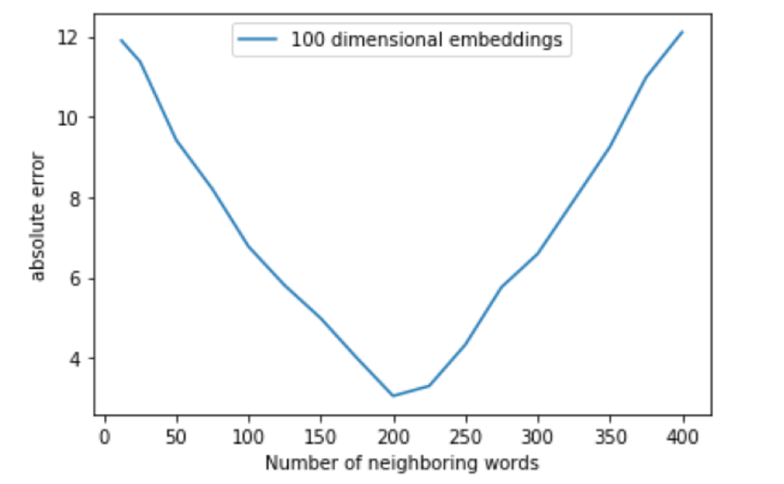
We see that for words with fewer senses, the optimal achievable relative error is 0.411 with word2vec embedding dimension of 500 and the number of neighbors considered is 25. For words with more senses, the optimal achievable relative error is 0.1897 with word2vec embedding dimension of 500 and number of neighbors considered is 200. We see that this is an interesting difference between the two groups. The relative error for words with fewer senses is positively correlated with the number of neighbors considered, i.e., as the number of neighbors goes down, so does the relative error. However, with words that have many senses, we see that there is a more complex interplay at work. We would expect that if we consider very few neighbors, we will not have enough information required to cluster all the senses and if we consider a very high number of neighbors, we expect to include a lot of irrelevant information for accurate clustering. Our intuition is that in both the above mentioned cases the error will be high. In Figure 3, we see that 200 neighbors is the clear minimum of words to be included to minimize the error of this system.
5 Future Work
Further we would like to implement the algorithm on different datasets such as SEMEVAL-2013, and SemCor+OMSTI (One Million Sense Tagged Instances) using different word embeddings like GloVe and FastText to observe the impact on the results.
We would also like to test our algorithm with pseudowords. For a word that has multiple meanings or senses, we can break that word up into its component senses, create new dummy words, and replace the original word with the respective dummy word. For example, if the word “foo” has two meanings, we can create words “foo$1” and “foo$2” and replace “foo” with the respective pseudoword we just created. Once we have done this, perhaps on some subset of the words in the datasets, we will replace the words in the corpora, retrain the embeddings, and rerun the barcode algorithm and infer the appropriateness of topological data analysis in word sense disambiguation/induction.
References
- Carpuat and Wu (2007) Marine Carpuat and Dekai Wu. 2007. Improving statistical machine translation using word sense disambiguation. In Proceedings of the 2007 Joint Conference on Empirical Methods in Natural Language Processing and Computational Natural Language Learning (EMNLP-CoNLL).
- Chazal (2016) Frédéric Chazal. 2016. High-dimensional topological data analysis.
- Edelsbrunner et al. (2000) Herbert Edelsbrunner, David Letscher, and Afra Zomorodian. 2000. Topological persistence and simplification. In Proceedings 41st Annual Symposium on Foundations of Computer Science, pages 454–463. IEEE.
- Edelsbrunner and Morozov (2012) Herbert Edelsbrunner and Dmitriy Morozov. 2012. Persistent homology: theory and practice. Technical report, Lawrence Berkeley National Lab.(LBNL), Berkeley, CA (United States).
- Frosini (1990) Patrizio Frosini. 1990. A distance for similarity classes of submanifolds of a euclidean space. Bulletin of the Australian Mathematical Society, 42(3):407–415.
- Ghrist (2018) Robert Ghrist. 2018. Homological algebra and data. Math. Data, 25:273.
- Lesnick (2013) Michael Lesnick. 2013. Studying the shape of data using topology. https://www.ias.edu/ideas/2013/lesnick-topological-data-analysis.
- Michel et al. (2017) Paul Michel, Abhilasha Ravichander, and Shruti Rijhwani. 2017. Does the geometry of word embeddings help document classification? a case study on persistent homology based representations. arXiv preprint arXiv:1705.10900.
- Mittal and Jain (2015) Kanika Mittal and Amita Jain. 2015. Word sense disambiguation method using semantic similarity measures and owa operator. ICTACT Journal on Soft Computing, 5(2).
- Morse (1940) Marston Morse. 1940. Rank and span in functional topology. Annals of Mathematics, pages 419–454.
- Perea (2018) Jose A Perea. 2018. A brief history of persistence. arXiv preprint arXiv:1809.03624.
- Robins (1999) Vanessa Robins. 1999. Towards computing homology from finite approximations. In Topology proceedings, volume 24, pages 503–532.
- Sami and Farrahi (2017) Ishrat Rahman Sami and Katayoun Farrahi. 2017. A simplified topological representation of text for local and global context. In Proceedings of the 25th ACM international conference on Multimedia, pages 1451–1456. ACM.
- Savle et al. (2019) Ketki Savle, Wlodek Zadrozny, and Minwoo Lee. 2019. Topological data analysis for discourse semantics? In Proceedings of the 13th International Conference on Computational Semantics-Student Papers, pages 34–43.
- Sinha and Mihalcea (2007) Ravi Sinha and Rada Mihalcea. 2007. Unsupervised graph-basedword sense disambiguation using measures of word semantic similarity. In International Conference on Semantic Computing (ICSC 2007), pages 363–369. IEEE.
- Temčinas (2018) Tadas Temčinas. 2018. Local homology of word embeddings. arXiv preprint arXiv:1810.10136.
- Wagner et al. (2012) Hubert Wagner, Paweł Dłotko, and Marian Mrozek. 2012. Computational topology in text mining. In Computational Topology in Image Context, pages 68–78. Springer.
- Zhu (2013) Xiaojin Zhu. 2013. Persistent homology: An introduction and a new text representation for natural language processing. In Twenty-Third International Joint Conference on Artificial Intelligence.