Bianchi Type I model of universe with customized scale factors

Pranjal Sarmah E-mail:p.sarmah97@gmail.com Affiliation: Department of Physics, Dibrugarh University, Dibrugarh 786004, Assam, India Umananda Dev Goswami E-mail:umananda2@gmail.com Affiliation: Department of Physics, Dibrugarh University, Dibrugarh 786004, Assam, India

Abstract

According to standard cosmology, the universe is homogeneous and isotropic at large scales. However, some anisotropies can be observed at the local scale in the universe through various ways. Here we have studied the Bianchi type I model with customizing the scale factors to understand the anisotropic nature of the universe. We have considered two cases with slight modifications of scale factors in different directions in the generalized Bianchi Type I metric equation, and compared the results with the $\Lambda$ CDM model and also with available cosmological observational data. Through this study, we also want to predict the possible degree of anisotropy present in the early universe and its evolution to current time by calculating the value of density parameter for anisotropy ( $\Omega_{\sigma}$ ) for both low and high redshift ( $z$ ) along with the possible relative anisotropy that exist among different directions. It is found that there was a relatively higher amount of anisotropy in the early universe and the anisotropic nature of the universe vanishes at the near past and the present epochs. Thus at near past and present stages of the universe there is no effective distinction between this anisotropic model and the standard $\Lambda$ CDM model.

Keywords:

Bianchi type I universe; anisotrpy; relative shear anisotropy; density parameter for anisotropy

I Introduction

The standard cosmology has assumed that the universe is exactly homogeneous and isotropic at large scales Tedesco_2018. The spacetime of this kind of universe is described by the Friedmann-Lemaître-Robertson-Walker (FLRW) metric, and it is assumed to be occupied by some ideal fluids with a diagonal energy momentum tensor Pebbles_1994; J.Colin_2019. Various cosmological observational data like, data of Type Ia Supernovae (SNe Ia) Hossienkhani_2021; Campanelli_2011; Akarsu_2019; Ma_2011; Tedesco_2018; Maurya_2018; Bamba_2012, Cosmic Microwave Background (CMB) Akarsu_2019; Bunn_1996; Costa_2004; Hossienkhani_2021; Ma_2011; Tedesco_2018; Campanelli_2011; Copi_2004; Eriksen_2004_a; Eriksen_2004_b, Baryon Acoustic Oscillation (BAO) Akarsu_2019; Hossienkhani_2021; Ma_2011; Tedesco_2018; Campanelli_2011, Hubble parameter Hossienkhani_2021; Campanelli_2011; Akarsu_2019; Ma_2011; Tedesco_2018; Maurya_2018; Frieman_2008; Perivolaropoulos_2014; Cea_2022, the Wilkinson Microwave Anisotropy Probe (WMAP) Hossienkhani_2021; Frieman_2008; Perivolaropoulos_2014; Buniy_2006; Campanelli_2006; Campanelli_2007; Berera_2004; Vielva_2004; Hansen_2004 and the Large Scale Structure (LSS) Hossienkhani_2021; Frieman_2008 etc. have suggested that the current expansion of the universe is accelerating Hossienkhani_2021; Ma_2011. This current accelerated expansion of the universe is considered to be due to the presence of a large negative pressure component in the universe, which is referred as the Dark Energy (DE). On the other hand, an unknown form of matter known as the Dark Matter (DM) is thought to be responsible for the formation of LSS in the universe J.Colin_2019; Hossienkhani_2018. However, at this point it would be appropriate to mention that according to the modified gravity theories scenario, the current accelerated expansion of the universe and DM are the manifestations of the modifications of spacetime behaviours at large scales, which could not be accounted for by the general theory of relativity Nojiri_2017; Gogoi_2021; Parbin_2021. Although the distribution of galaxies under the background of dominated DM is observed to be inhomogeneous J.Colin_2019, other observational sources like different galaxy redshift catalogues have suggested a statistical transition from the inhomogeneity to homogeneity on scale exceeding $\sim$ 100 Mpc J.Colin_2019; Hogg_2005; Scrimgeour_2012. Thus, the assumption of isotropy and homogeneity of the universe is applicable only for the large scales Tedesco_2018. However, the standard cosmological models are challenged by few other puzzling cosmological observations Perivolaropoulos_2014; Wang_2018, such as power asymmetry of the CMB perturbation maps (Eriksen H. K_2007; Hoftuft_2009; Paci_2010; Mariano_2013; Zhao_2016), anisotropy in accelerating expansion rate Antoniou_2010; Mariano_2012; Wang_2014, the large scale velocity flow Kashlinsky_2010; Kashlinsky_2008; Watkins_2009; Feldman_2010; Lavaux_2010, spatial dependence of the value of the fine structure constant Perivolaropoulos_2014; Moss_2011; Webb_2011; King_2012; Pinho_2016, etc. Based on the observations of these cosmic anomalies Perivolaropoulos_2014, the Planck collaboration had rightly stated that “The Universe is still weird and interesting” Zhao_2016. The origin of these anomalies are still unknown. These may either be arised due to the large statistical fluctuations or may have some physical origin like geometry or energy of the universe Perivolaropoulos_2014 or may favour of a preferred cosmological direction, and perhaps depict the anisotropic nature of the universe.

Testing the large-scale geometry of the universe by using cosmological scale is one of the major challenges of modern cosmology Campanelli_2011. Reliable observational data from the various sources like WMAP, BAO, Planck Planck_2018 etc. have given new insight on the study of the basic assumptions (i.e. isotropy and homogeneity) of the standard cosmological models and also shown the anisotropic characteristics of the universe at least at the local scale. In our real universe, there exist some kind of strange motions due to the local inhomogeneity and anisotropy of surrounding structures, which can not be neglected J.Colin_2019. To explain the anisotropic character of the universe, spatially homogeneous and anisotropic cosmological models play a significant role to describe the large-scale behaviour of the universe. These models have been widely studied under the regime of general relativity to understand the relativistic picture of the universe at its early stage Maurya_2018. Thus, we need a simple and convincing cosmological model with a relativistic background metric Akarsu_2019, which allows directional scale factors Akarsu_2019; Tedesco_2018; Campanelli_2011; Maurya_2018; Paul_2008 while maintaining the spatial homogeneity and flatness. The Bianchi Type I model Akarsu_2019; Tedesco_2018; Maurya_2018; Campanelli_2011; Hossienkhani_2018; Paul_2008; Perivolaropoulos_2014 and its metric fulfill the above criteria and hence it is suitable for study the anisotropic nature of the universe in its early stages as well as in the current scenario. Bianchi Type I model describes the anisotropic nature of the universe by considering the anisotropic and homogeneous background Tedesco_2018. It gives a very small deviation from the exact isotropy. Hence, use of Bianchi Type I geometry corresponds to replacing the spatially flat FLRW background by Bianchi Type I background metric Tedesco_2018. Therefore, the Bianchi Type I geometry can be considered as an alternative option to the FLRW metric to study the various cosmic anomalies as mentioned above.

Keeping in view of the above points, in this study, we have used the Bianchi Type I metric (Akarsu_2019; Maurya_2018; Hossienkhani_2018; Paul_2008; Perivolaropoulos_2014) with the “customized scale factors” in different directions. Here we have considered two cases. For case I, we have modified directional scale factors in the Bianchi type I metric by considering the second and third scale factors in terms of the first one with some multiplicative constants. For case II, we have again considered the second and third scale factors in terms of the first one, but here we have added constant terms with them rather than multiplying. With these two cases of scale factors in the metric, we have derived various cosmological parameters Tedesco_2018; Akarsu_2019; Maurya_2018; Perivolaropoulos_2014; Frieman_2008; Hossienkhani_2018; Gogoi_2021; Paul_2008; Barrow_1997 including the directional Hubble parameters, average or mean Hubble parameter, deceleration parameter, shear scalar, relative shear anisotropy parameter or Hubble normalized shear parameter, average anisotropic expansion, density parameters (matter, radiation, anisotropy and dark energy), distance modulus, Equation of State (EoS) etc. We have also studied the evolution of various cosmological parameters with respect to cosmological redshift ( $z$ ) Frieman_2008; Gogoi_2021; Hossienkhani_2018 by plotting those parameters against $z$ or ( $1+z$ ) and compared them with the standard cosmological model ( $\Lambda$ CDM model) and also with the available observational data of various sources for both the cases.

This paper is organized as follows. In Section II, the basics of the Bianchi Type I model have been discussed. Here, we have mainly included the various mathematical equations and expressions of the Bianchi type I universe from various literatures. In Section III, we have derived all the mathematical equations and expressions using the “customized scale factors approach” for the Bianchi Type I model of the universe. This section is subdivided into two subsections III.1 and III.2, in which we have derived all the expressions and equations for two separate cases respectively. In Section IV, we have made graphical analysis of the various cosmological parameters with respect to $z$ and tried to give the explanations of those results obtained from the plots for both the cases. The paper has been summarized in Section V with conclusions. Throughout this work we use the geometrized unit system, where $c=G=1$ with $(-,+,+,+)$ metric convention.

II Basic equations of Bianchi type I model

The general form of the metric for the Bianchi Type I universe Perivolaropoulos_2014; Akarsu_2019; Paul_2008; Maurya_2018; Hossienkhani_2018 can be written as

ds^{2}=-\,dt^{2}+\sum_{i=1}^{3}a_{i}(dx^{i})^{2},

(1)

where $a_{i}$ is the directional scale factor along the $i$ th direction, which is the function of time $t$ only. The average expansion scale factor $(a_{1}a_{2}a_{3})^{\frac{1}{3}}$ arises from the average Hubble parameter defined as

H=\frac{1}{3}{\sum\limits_{i=1}^{3}H_{i}}

with $H_{i}=\frac{\dot{a_{i}}}{a_{i}}$ is the directional Hubble parameter along the $i$ th direction The most general form of the energy-momentum tensor $T_{\mu\nu}$ for the given metric can be considered in the form:

T_{\mu}^{\nu}=diag\big[-\rho,P,P,P\big],

(2)

where $\rho$ is the energy density and $P$ is the isotropic pressure of a perfect fluid. Now, in view of the present scenario of our accelerating universe, we consider the Einstein field equations with the cosmological constant $\Lambda$ as

R_{\mu\nu}-\frac{1}{2}g_{\mu\nu}R+\Lambda g_{\mu\nu}=8\pi T_{\mu\nu},

(3)

where $R_{\mu\nu}$ is the Ricci tensor, R is the Ricci scalar and $g_{\mu\nu}$ is the metric tensor. For the above metric (1) and the energy-momentum tensor (2), the following set of field equations can be obtained from the Einstein field equations:

$\displaystyle H_{1}H_{2}+H_{1}H_{3}+H_{2}H_{3}$	$\displaystyle=8\pi\rho+\Lambda,$	(4)
$\displaystyle\frac{\ddot{a_{2}}}{a_{2}}+\frac{\ddot{a_{3}}}{a_{3}}+H_{2}H_{3}$	$\displaystyle=-\,8\pi P+\Lambda,$	(5)
$\displaystyle\frac{\ddot{a_{3}}}{a_{3}}+\frac{\ddot{a_{1}}}{a_{1}}+H_{3}H_{1}$	$\displaystyle=-\,8\pi P+\Lambda,$	(6)
$\displaystyle\frac{\ddot{a_{1}}}{a_{1}}+\frac{\ddot{a_{2}}}{a_{2}}+H_{1}H_{2}$	$\displaystyle=-\,8\pi P+\Lambda.$	(7)

Combining Eqs. (5), (6) and (7) and then subtracting Eq. (4) from the combined one, we may write the resulting Friedmann equation as

\sum_{i=1}^{3}\frac{\ddot{a_{i}}}{a_{i}}=-\,4\pi\big(3P+\rho\big)+\Lambda.

(8)

The continuity equation in this model of the universe is given by Paul_2008,

\dot{\rho}+\big(\rho+P\big)\sum_{i=1}^{3}\frac{\dot{a}_{i}}{a_{i}}=0.

(9)

Considering the EoS $P=\omega\rho$ in Eq. (9), in which the parameter $\omega$ tells us about the nature of energy or matter density in the universe, for example, $\omega=0$ for the non-relativistic matter, $\omega=\frac{1}{3}$ for the radiation and $\omega=-1$ for the vacuum energy Frieman_2008; Maurya_2018; Akarsu_2019, the energy density of the universe can be found as

\rho=\rho_{0}\prod_{i=1}^{3}a_{i}^{-(1+\omega)}.

(10)

Here $\rho_{0}$ is the present energy density of the universe. From this equation it is seen that the future energy density of this model of the universe is the EoS parameter $\omega$ dependent, i.e. on the nature of the matter or energy content of the universe. It is clear that $\rho\propto(a_{1}a_{2}a_{3})^{-1}$ for the matter, $\rho\propto(a_{1}a_{2}a_{3})^{-\frac{4}{3}}$ for the radiation and $\rho=\rho_{0}$ (constant) for the vacuum energy dominated cases respectively.

Using Eq. (4) the Hubble parameter of this universe can be expressed in terms of the present density parameters of the universe as

H=H_{0}{\sqrt{\Omega_{m0}(a_{1}a_{2}a_{3})^{-1}+\Omega_{r0}(a_{1}a_{2}a_{3})^{-\frac{4}{3}}+\Omega_{\Lambda 0}+\Omega_{\sigma 0}(a_{1}a_{2}a_{3})^{-2}}},

(11)

where $H_{0}$ is the current Hubble parameter, and $\Omega_{m0}=8\pi\rho_{m0}/3H_{0}^{2}$ is the density parameters for the matter content, $\Omega_{r0}=8\pi\rho_{r0}/3H_{0}^{2}$ is the density parameter for the radiation content, $\Omega_{\Lambda 0}=\Lambda/3H_{0}^{2}$ is the density parameter for the vacuum energy and $\Omega_{\sigma 0}=\sigma_{0}^{2}/3H_{0}^{2}$ is the density parameter for the anisotropy Akarsu_2019; Maurya_2018; Hossienkhani_2021 of the present universe. Here, $\rho_{m0}$ and $\rho_{r0}$ are current values of matter density $\rho_{m}$ and radiation density $\rho_{r}$ of the universe respectively. The term $\sigma_{0}^{2}$ in $\Omega_{\sigma 0}$ is the current value of shear scalar. The shear scalar is the parameter through which the contribution of the expansion anisotropy in Bianchi type I model of universe can be quantified. It arises due to the different scale factor taken for different directions in the Bianchi model of universe. For the isotropic case, $\sigma_{0}^{2}=0$ . The current value of shear scalar, i.e. $\sigma_{0}^{2}$ is related with the shear scalar $\sigma^{2}$ by the relation $\sigma^{2}=\sigma_{0}^{2}(a_{1}a_{2}a_{3})^{-2}$ . In general the shear scalar $\sigma^{2}$ in terms of the average and directional Hubble parameters can be written as Maurya_2018; Akarsu_2019; Paul_2008

\sigma^{2}=\frac{1}{2}\Big[\sum_{i=1}^{3}H_{i}^{2}-3H^{2}\Big].

(12)

Again, the deceleration parameter for the Bianchi Type I universe can be derived as

q=-\frac{1}{3H^{2}}\bigg(\frac{\ddot{a}_{1}}{a_{1}}+\frac{\ddot{a}_{2}}{a_{2}}+\frac{\ddot{a}_{3}}{a_{3}}\bigg)+\frac{2\sigma^{2}}{3H^{2}}.

(13)

Using Eq. (8) and the EoS mentioned above, this equation for the deceleration parameter $q$ can expressed in terms of density parameters of the universe as

q=\frac{1}{2}\Omega_{m}+\Omega_{r}-\Omega_{\Lambda}+2\,\Omega_{\sigma},

(14)

where $\Omega_{m}=8\pi\rho_{m}/3H^{2}$ , $\Omega_{r}=8\pi\rho_{r}/3H^{2}$ , $\Omega_{\Lambda}=\Lambda/3H^{2}$ and $\Omega_{\sigma}=\frac{\sigma^{2}}{3H^{2}}$ Akarsu_2019 are the matter density parameter, radiation density parameter, vacuum energy density parameter and anisotropy or shear density parameter respectively of the universe at any given instant. Similarly, the average anisotropic expansion Maurya_2018; Paul_2008 for Bianchi type I universe is

A=\frac{1}{3}\sum_{i=1}^{3}\Big(\,\frac{\Delta H_{i}}{H}\Big)^{2}=2\,\Omega_{\sigma},\;\;\Delta H_{i}=(H_{i}-H).

(15)

The cosmological redshift ( $z$ ) is another cosmological parameter, which is a very important parameter to understand the evolution and history of the universe in the sense that it is a directly observable parameter, not the scale factor. Hence to quantify the effect of anisotropy in the observable domain of the universe, it is necessary to express all other cosmological parameters mentioned above as the functions of $z$ . In this context, it is to be noted that in the case of the Bianchi type I universe, there exist three redshifts in three spatial directions due to the directional dependence of scale factor. If $z_{1},z_{2},z_{3}$ are these three redshift parameters along three spatial directions, then they can be defined as

\frac{a_{1}(t)}{a_{10}}=\frac{1}{1+z_{1}},\;\;\frac{a_{2}(t)}{a_{20}}=\frac{1}{1+z_{2}}\;\;\mbox{and}\;\;\frac{a_{3}(t)}{a_{30}}=\frac{1}{1+z_{3}}.

(16)

Here, $a_{10},a_{20},a_{30}$ are the scale factors of present time along the three spatial directions. Now, from the current observations, we have taken $a_{10}=a_{20}=a_{30}=1$ Maurya_2018 and thus the scale factors can be rewritten in terms of $z_{1},z_{2},z_{3}$ as

a_{1}(t)=\frac{1}{1+z_{1}},\;\;{a_{2}(t)}=\frac{1}{1+z_{2}}\;\;\mbox{and}\;\;{a_{3}(t)}=\frac{1}{1+z_{3}}.

(17)

With this form of the scale factors, the directional Hubble parameters ( $H_{i})$ can be written in terms of $z_{i}$ as

H_{i}=-\,\frac{\dot{z}_{i}}{1+z_{i}}

(18)

and hence the average Hubble parameter takes the form:

H=-\frac{1}{3}\sum_{i=1}^{3}\frac{\dot{z}_{i}}{1+z_{i}}.

(19)

Thus, Eq. (11) for the average Hubble parameter can be rewritten in terms of redshift parameters $(z_{1},z_{2},z_{3})$ as

H=H_{0}\sqrt{E(z_{1},z_{2},z_{3})},

(20)

\!\!\!\!\!\!\!\mbox{where}\;\;E(z_{1},z_{2},z_{3})=\Omega_{m0}\big[(1+z_{1})(1+z_{2})(1+z_{3})\big]\\ +\Omega_{r0}\big[(1+z_{1})(1+z_{2})(1+z_{3})\big]^{\frac{4}{3}}+\Omega_{\Lambda 0}+\Omega_{\sigma 0}\big[(1+z_{1})(1+z_{2})(1+z_{3})\big]^{2}.

(21)

With the help of Eqs. (18), (19) and (20), the age of the universe can be expressed in terms of the directional redshift parameters $(z_{1},z_{2},z_{3})$ as follows:

t_{age}=\int_{0}^{t}dt=\frac{1}{3H_{0}}\Bigg[\int_{0}^{\infty}\frac{dz_{1}}{(1+z_{1})\sqrt{E(z_{1},z_{2},z_{3})}}+\int_{0}^{\infty}\frac{dz_{2}}{(1+z_{2})\sqrt{E(z_{1},z_{2},z_{3})}}+\int_{0}^{\infty}\frac{dz_{3}}{(1+z_{3})\sqrt{E(z_{1},z_{2},z_{3})}}\Bigg].

(22)

Other cosmological parameters in terms of redshift can be derived for this model of the universe as follows:

(i) Deceleration parameter:

q(z_{1},z_{2},z_{3})=\frac{1}{E(z_{1},z_{2},z_{3})}\bigg[\frac{1}{2}\,\Omega_{m0}\,(1+z_{1})(1+z_{2})(1+z_{3})+\Omega_{r0}\Big\{(1+z_{1})(1+z_{2})(1+z_{3})\Big\}^{\frac{4}{3}}\\ -\,\Omega_{\Lambda 0}+2\,\Omega_{\sigma 0}\Big\{(1+z_{1})(1+z_{2})(1+z_{3})\Big\}^{2}\bigg].

(23)

(ii) Equation of State:

\omega(z_{1},z_{2},z_{3})=\frac{\frac{1}{3}\,\Omega_{r0}\big[(1+z_{1})(1+z_{2})(1+z_{3})\big]^{\frac{4}{3}}-\Omega_{\Lambda 0}}{\Omega_{m0}\big[(1+z_{1})(1+z_{2})(1+z_{3})\big]+\Omega_{r0}\big[(1+z_{1})(1+z_{2})(1+z_{3})\big]^{\frac{4}{3}}+\Omega_{\Lambda 0}}.

(24)

(iii) Ricci Scalar:

R(z_{1},z_{2},z_{3})=3H_{0}^{2}\Big[\Omega_{m0}(1+z_{1})(1+z_{2})(1+z_{3})+4\,\Omega_{\Lambda 0}\Big].

(25)

(iv) Luminosity distance:

d_{L}(z_{1},z_{2},z_{3})=\frac{\big[(1+z_{1})(1+z_{2})(1+z_{3})\big]^{\frac{1}{3}}}{3H_{0}}\int_{0}^{\infty}\Big\{\frac{\big[(1+z_{2})(1+z_{3})\big]^{\frac{1}{3}}}{(1+z_{1})^{\frac{2}{3}}\sqrt{E(z_{1},z_{2},z_{3})}}\,dz_{1}+\frac{\big[(1+z_{1})(1+z_{3})\big]^{\frac{1}{3}}}{(1+z_{2})^{\frac{2}{3}}\sqrt{E(z_{1},z_{2},z_{3})}}\,dz_{2}\\ +\frac{\big[(1+z_{1})(1+z_{2})\big]^{\frac{1}{3}}}{(1+z_{3})^{\frac{2}{3}}\sqrt{E(z_{1},z_{2},z_{3})}}\,dz_{3}\Big\}.

(26)

(v) Distance Modulus:

D_{m}=5\log{d_{L}}+25.

(27)

These are some important expressions in general Bianchi Type I cosmology in generic form, which will be useful to study the properties of the universe in terms of the observable parameter $z$ for our considered cases as discussed in the following sections.

III Customized scale factor approach for Bianchi Type I model

In this section we implement two different cases to the Bianchi type I model for which we use two different types of directional scale factors to calculate the various cosmological parameters as discussed below.

III.1 Case I

In this case we consider the following set of directional scale factors:

a_{1}=a(t),\;\;a_{2}=\alpha\,a(t),\;\;\mbox{and}\;\;a_{3}=\beta\,a(t),

(28)

where $\alpha$ and $\beta$ are two multiplicative constants. Since $\alpha$ and $\beta$ are two time independent constants, the directional dependence of scale factors or the anisotropy in the universe in this case should be considerable only for very small values of the scale factor $a(t)$ , i.e. for the cosmological redshift $z\gg 1$ . The major advantage of these forms of scale factors is that we can express every equation and cosmological parameter in terms of a single scale factor multiplied by some constants. It helps to simplify the problem and hence reduces the complexity. The directional Hubble parameters for the above considered set of scale factors take the same form as in the case of the isotropic situation, i.e.

H_{1}=H_{2}=H_{3}=\frac{\dot{a}}{a},

(29)

and consequently the average Hubble parameter is

H=\frac{\dot{a}}{a}.

(30)

Also it can be easily seen that

\frac{\ddot{a}_{1}}{a_{1}}=\frac{\ddot{a}_{2}}{a_{2}}=\frac{\ddot{a}_{3}}{a_{3}}=\frac{\ddot{a}}{a}.

(31)

Thus the temporal component of the Einstein field equations, i.e. Eq. (4) is transformed for this case as

H^{2}=\frac{8\pi\rho}{3}+\frac{\Lambda}{3}.

(32)

Whereas all the three spatial components of the Einstein field equations, given in Eqs. (5), (6), (7) take the same form for this case as

2\,\frac{\ddot{a}}{a}+H^{2}=-\,8\pi P+\Lambda,

(33)

and hence the combination of all the three spatial field equations leads to the equation:

6\,\frac{\ddot{a}}{a}+3H^{2}=-\,8\pi\,(3P)+3\Lambda.

(34)

Now multiplication of Eq. (32) by a factor $3$ and then subtracting it from Eq. (34) give rise a new equation:

\frac{\ddot{a}}{a}=-\frac{4\pi\,(\rho+3P)}{3}+\frac{\Lambda}{3}.

(35)

It should be pointed out that this Eq. (35) can also be derived directly from Eq. (8). Eqs. (32) and (35) are the two independent form of field equations. Similarly the Eq. (9) i.e. the continuity equation can be rewritten in this case as

\dot{\rho}+3\,{\frac{\dot{a}}{a}}\,(\rho+P)=0.

(36)

Again Eq. (10), i.e. the expression of energy density for this case becomes,

\rho=(\alpha\beta)^{-(1+\omega)}{\rho_{0}}\,{a^{-3(1+\omega)}}.

(37)

It is clear that this expression is different from the isotropic situation as it depends on the parameters $\alpha$ and $\beta$ . Hence, although the expressions for directional and average Hubble parameters, and some other expressions derived above look identical to the isotropic situation, they would behave differently because of the different form of the energy density in this case. This can be seen clearly from the expression (11) for the Hubble parameter, which can rewritten for this case as

H=H_{0}{\sqrt{(\alpha\beta)^{-1}\Omega_{m0}\,a^{-3}+(\alpha\beta)^{-\frac{4}{3}}\Omega_{r0}\,a^{-4}+\Omega_{\Lambda 0}}}.

(38)

Here $\Omega_{\sigma}=0$ as $\sigma^{2}=0$ from Eq. (12) for this case. We see that the matter and radiation parts of energy density contributed differently in the Hubble parameter than the isotropic condition because of the expression (37) for the energy density. This situation will be similar to all other cosmological parameters discussed here. The deceleration parameter of Eq. (13) in this case reduces to

q=-\frac{\ddot{a}}{aH^{2}}.

(39)

And in terms of density parameter, $q$ can be rewritten as

q=\Omega_{r}+\frac{1}{2}\,\Omega_{m}-\Omega_{\Lambda}.

(40)

If we denote $z_{1}=z$ , the relations between the cosmological redshift parameters and the directional scale factors given in Eq. (17) will be transformed in this case as

a_{1}(t)=\frac{1}{1+z},\;\;{a_{2}(t)}=\frac{\alpha}{1+z},\;\;\mbox{and}\;\;{a_{3}(t)}=\frac{\beta}{1+z}.

(41)

Here, the other two redshift parameters $z_{2}$ and $z_{3}$ can be found as

z_{2}=\frac{1+z}{\alpha}-1,\;\;\mbox{and}\;\;z_{3}=\frac{1+z}{\beta}-1.

Accordingly, the directional Hubble parameters can be written as

H_{i}=-\frac{\dot{z}}{1+z}.

(42)

and hence the form of the expression of the average Hubble parameter becomes exactly the same as the directional Hubble parameters’ expression given above. Thus, in terms of the cosmological redshift parameters Eq. (38) can be rewritten as

H=H_{0}{\sqrt{(\alpha\beta)^{-1}\Omega_{m0}(1+z)^{3}+(\alpha\beta)^{-\frac{4}{3}}\Omega_{r0}(1+z)^{4}+\Omega_{\Lambda 0}}}\;\;=H_{0}\sqrt{E(z)},

(43)

where

E(z)=(\alpha\beta)^{-1}\Omega_{m0}(1+z)^{3}+(\alpha\beta)^{-\frac{4}{3}}\Omega_{r0}(1+z)^{4}+\Omega_{\Lambda 0}.

(44)

Consequently, the age of the universe given by Eq. (22) can be rewritten for this case as

t_{age}=\int_{0}^{t}dt=\frac{1}{H_{0}}\int_{0}^{\infty}\frac{dz}{(1+z)\sqrt{E(z)}}.

(45)

Similarly, with the same approach the other cosmological parameters for the present case can be obtained as a function of redshift parameters as

(i) Deceleration parameter:

q(z)=\frac{1}{\sqrt{E(z)}}\Big[\frac{1}{2}(\alpha\beta)^{-1}\Omega_{m0}(1+z)^{3}+(\alpha\beta)^{-\frac{4}{3}}\Omega_{r0}(1+z)^{4}-\Omega_{\Lambda 0}\Big].

(46)

(ii) Equation of State:

\omega(z)=\frac{\frac{1}{3}\Omega_{r0}(\alpha\beta)^{-\frac{4}{3}}(1+z)^{4}-\Omega_{\Lambda 0}}{(\alpha\beta)^{-1}\Omega_{m0}(1+z)^{3}+\Omega_{r0}(\alpha\beta)^{-\frac{4}{3}}(1+z)^{4}+\Omega_{\Lambda 0}}.

(47)

(iii) Ricci Scalar:

R(z)=3H_{0}^{2}\Big[(\alpha\beta)^{-1}\Omega_{m0}(1+z)^{3}+4\Omega_{\Lambda 0}\Big].

(48)

(iv) Luminosity distance:

d_{L}=\frac{(\alpha\beta)^{-\frac{2}{3}}(1+z)}{H_{0}}\int_{0}^{\infty}\frac{dz}{\sqrt{E(z)}}.

(49)

(v) Density parameter of matter:

\Omega_{m}(z)=\frac{\Omega_{m0}(\alpha\beta)^{-1}(1+z)^{3}}{E(z)}.

(50)

These are the forms of expressions of the cosmological parameters we have obtained for the given set of scale factors in Eq. (28). The detailed analysis of these expressions are done graphically in section IV.

III.2 Case II

In this case we consider that scale factors of the three dimensional universe differ from each other by some constant amounts and hence here we consider the following set of anisotropic scale factors:

a_{1}=a(t),\;\;a_{2}=a(t)+\delta,\;\;\mbox{and}\;\;a_{3}=a(t)+\gamma,

(51)

where $\delta$ and $\gamma$ are two constants. As in the previous case, these form of scale factors help us to reduce the complexity and hence easier to deal with the problem. For convenience, this set of scale factors can also be written as

a_{1}=a(t),\;\;a_{2}=a(t)f_{a\delta},\;\;\mbox{and}\;\;a_{3}=a(t)f_{a\gamma},

(52)

where $f_{a\delta}=1+\delta/a(t)$ and $f_{a\gamma}=1+\gamma/a(t)$ . It is clear that $f_{a\delta},f_{a\gamma}\rightarrow 1$ , when the scale factor $a(t)\rightarrow\infty$ or the cosmological redshift $z\rightarrow-1$ . On the other hand when $a(t)\rightarrow 0$ or $z\gg 1$ , $f_{a\delta}$ , $f_{a\gamma}\gg 1$ . Thus, according to this case the universe will be almost in an isotropic state in the distant future and the anisotropy in the universe was significant in the distant past as in the case I. With this set of scale factors (52) the directional Hubble parameters of the anistropic universe becomes:

H_{1}=\frac{\dot{a}}{a},\;\;H_{2}=\frac{H_{1}}{f_{a\delta}},\;\;H_{3}=\frac{H_{1}}{f_{a\gamma}}

(53)

and hence the average Hubble parameter can be written as

H=\frac{H_{1}}{3}\Big[1+f_{a\delta}^{-1}+f_{a\gamma}^{-1}\Big].

(54)

Again,

\frac{\ddot{a}_{1}}{a_{1}}=\frac{\ddot{a}}{a},\;\;\frac{\ddot{a}_{2}}{a_{2}}=\frac{\ddot{a}}{a}\,f_{a\delta}^{-1},\;\;\frac{\ddot{a}_{3}}{a_{3}}=\frac{\ddot{a}}{a}\,f_{a\gamma}^{-1}.

(55)

The Einstein field equations as mentioned in Eqs. (4), (5), (6) and (7) are transformed for the present case as

$\displaystyle H_{1}^{2}\Big[f_{a\delta}^{-1}+f_{a\gamma}^{-1}+\big(f_{a\delta}f_{a\gamma}\big)^{-1}\Big]$	$\displaystyle=8\pi\rho+\Lambda,$	(56)
$\displaystyle\frac{\ddot{a}}{a}\Big[f_{a\delta}^{-1}+f_{a\gamma}^{-1}\Big]+H_{1}^{2}\big(f_{a\delta}f_{a\gamma}\big)^{-1}$	$\displaystyle=-\,8\pi P+\Lambda,$	(57)
$\displaystyle\frac{\ddot{a}}{a}\Big[1+f_{a\gamma}^{-1}\Big]+H_{1}^{2}\,f_{a\gamma}^{-1}$	$\displaystyle=-\,8\pi P+\Lambda,$	(58)
$\displaystyle\frac{\ddot{a}}{a}\Big[1+f_{a\delta}^{-1}\Big]+H_{1}^{2}\,f_{a\delta}^{-1}$	$\displaystyle=-\,8\pi P+\Lambda.$	(59)

And Eq. (8) can be rewritten as

\frac{\ddot{a}}{a}\Big[1+f_{a\delta}^{-1}+f_{a\gamma}^{-1}\Big]=-\,4\pi(3P+\rho)+\Lambda.

(60)

The continuity equation for this case becomes,

\dot{\rho}+\big(\rho+P\big)H_{1}\Big[1+f_{a\delta}^{-1}+f_{a\gamma}^{-1}\Big]=0

(61)

and the energy density Eq. (10) can be rewritten as

\rho=\rho_{0}\big(f_{a\delta}f_{a\gamma})^{-(1+\omega)}a^{-3(1+\omega)}.

(62)

Similarly, the expression of shear scalar takes the form:

\sigma^{2}=\frac{H_{1}^{2}}{3}\bigg[1+f_{a\delta}^{-2}+f_{a\gamma}^{-2}-\Big(f_{a\delta}^{-1}+f_{a\gamma}^{-1}+\big(f_{a\delta}f_{a\gamma}\big)^{-1}\Big)\bigg].

(63)

This expression of shear scalar can be used to calculate the density parameter for anisotropy, $\Omega_{\sigma}=\sigma^{2}/3H^{2}$ . The Hubble parameter expression (11) for this case can be found as

H=H_{0}\sqrt{\Omega_{mo}\big(f_{a\delta}f_{a\gamma}\big)^{-1}a^{-3}+\Omega_{ro}\big(f_{a\delta}f_{a\gamma}\big)^{-\frac{4}{3}}a^{-4}+\Omega_{\Lambda 0}+\Omega_{\sigma 0}\big(f_{a\delta}f_{a\gamma}\big)^{-2}a^{-6}}

(64)

The deceleration parameter of Eq. (13) for the present case takes the form:

q=-\frac{1}{3H^{2}}\frac{\ddot{a}}{a}\Big[1+f_{a\delta}^{-1}+f_{a\gamma}^{-1}\Big]+2\,\Omega_{\sigma}.

(65)

However, the expression of $q$ in terms of density parameters is same as Eq. (14).

As in the case I, in this case also all cosmological parameters need to be expressed in terms of the cosmological redshift parameter, which is an observable quantity. The relation between cosmological redshift parameters and directional scale factors in this present case will take the form:

a_{1}(t)=\frac{1}{1+z},\;\;{a_{2}(t)}=\frac{1}{1+z}+\delta,\;\;\mbox{and}\;\;{a_{3}(t)}={\frac{1}{1+z}}+\gamma.

(66)

As earlier, for the convenient notational purpose this set of scale factors can also be re-expressed as

a_{1}(t)=\frac{1}{1+z},\;\;{a_{2}(t)}=\frac{f_{z\delta}}{1+z},\;\;\mbox{and}\;\;{a_{3}(t)}={\frac{f_{z\gamma}}{1+z}},

(67)

where $f_{z\delta}=1+(1+z)\delta$ and $f_{z\gamma}=1+(1+z)\gamma$ . Indeed, the behaviours of $f_{z\delta}$ and $f_{z\gamma}$ are exactly same as $f_{a\delta}$ and $f_{a\gamma}$ for different values of $z$ as discussed above. Here the directional cosmological redshift parameters $z_{2}$ and $z_{3}$ can be obtained as

z_{2}=\frac{1+z}{f_{z\delta}}-1,\;\;\mbox{and}\;\;z_{3}=\frac{1+z}{f_{z\gamma}}-1.

For this set of scale factors the directional Hubble parameters can be written as

H_{1}=-\frac{\dot{z}}{1+z},\;\;H_{2}=-\,\frac{\dot{z}}{(1+z)f_{z\delta}},\;\;H_{3}=-\,\frac{\dot{z}}{(1+z)f_{z\gamma}}.

(68)

Thus the expression of average Hubble parameter takes the form:

H=-\frac{\dot{z}}{3(1+z)}\Big[1+f_{z\delta}^{-1}+f_{z\gamma}^{-1}\Big].

(69)

In view of the above set of scale factors, Eq. (64) can now be rewritten as

H=H_{0}\sqrt{E(z)},

(70)

where

E(z)=\Omega_{m0}\big(f_{z\delta}f_{z\gamma}\big)^{-1}(1+z)^{3}+\Omega_{r0}\big(f_{z\delta}f_{z\gamma}\big)^{-\frac{4}{3}}(1+z)^{4}+\Omega_{\Lambda 0}+\Omega_{\sigma 0}\big(f_{z\delta}f_{z\gamma}\big)^{-2}(1+z)^{6}.

(71)

Correspondingly, the age of the universe can be written as

t_{age}=\frac{1}{H_{0}}\int_{0}^{\infty}\frac{dz}{(1+z)\sqrt{E(z)}}-\frac{1}{3H_{0}}\int_{0}^{\infty}\Big[\frac{\delta}{f_{z\delta}\sqrt{E(z)}}+\frac{\gamma}{f_{z\gamma}\sqrt{E(z)}}\Big]dz.

(72)

As before, other cosmological parameters in terms of redshift are as follows:

(i) Deceleration parameter:

q(z)=\frac{1}{\sqrt{E(z)}}\Big[\frac{1}{2}\,\Omega_{m0}\big(f_{z\delta}f_{z\gamma}\big)^{-1}(1+z)^{3}+\Omega_{r0}\big(f_{z\delta}f_{z\gamma}\big)^{-\frac{4}{3}}(1+z)^{4}+\Omega_{\Lambda 0}+2\Omega_{\sigma 0}\big(f_{z\delta}f_{z\gamma}\big)^{-2}(1+z)^{6}\Big].

(73)

(ii) Equation of State:

\omega(z)=\frac{\frac{1}{3}\Omega_{r0}\big(f_{z\delta}f_{z\gamma}\big)^{-\frac{4}{3}}(1+z)^{4}-\Omega_{\Lambda 0}}{\Omega_{m0}\big(f_{z\delta}f_{z\gamma}\big)^{-1}(1+z)^{3}+\Omega_{r0}\big(f_{z\delta}f_{z\gamma}\big)^{-\frac{4}{3}}(1+z)^{4}+\Omega_{\Lambda 0}}.

(74)

(iii) Ricci Scalar:

R(z)=3H_{0}^{2}\Big[\Omega_{m0}\big(f_{z\delta}f_{z\gamma}\big)^{-1}(1+z)^{3}+4\,\Omega_{\Lambda 0}\Big].

(75)

(iv) Luminosity distance:

d_{L}(z)=\frac{\big(f_{z\delta}f_{z\gamma}\big)^{-\frac{1}{3}}(1+z)}{H_{0}}\int_{0}^{\infty}\bigg[\frac{1}{\big(f_{z\delta}f_{z\gamma}\big)^{\frac{1}{3}}\sqrt{E(z)}}-\frac{\delta(1+z)}{3\,f_{z\delta}^{\frac{4}{3}}f_{z\gamma}^{\frac{1}{3}}\sqrt{E(z)}}-\frac{\gamma(1+z)}{3\,f_{z\delta}^{\frac{1}{3}}f_{z\gamma}^{\frac{4}{3}}\sqrt{E(z)}}\bigg]dz.

(76)

(vi) Density parameter for anisotropy:

\Omega_{\sigma}=\frac{AB}{CE(z)},

(77)

where $A=\Omega_{m0}\big(f_{z\delta}f_{z\gamma}\big)^{-1}(1+z)^{3}+\Omega_{r0}\big(f_{z\delta}f_{z\gamma}\big)^{-\frac{4}{3}}(1+z)^{4}+\Omega_{\Lambda 0}$ , $B=1+f_{z\delta}^{-2}+f_{z\gamma}^{-2}-\Big[f_{z\delta}^{-1}+f_{z\gamma}^{-1}+\big(f_{z\delta}f_{z\gamma}\big)^{-1}\Big]$ and $C=f_{z\delta}^{-1}+f_{z\gamma}^{-1}+\big(f_{z\delta}f_{z\gamma}\big)^{-1}$ .

(vii) Density parameter for matter:

\Omega_{m}(z)=\frac{\Omega_{m0}\big(f_{z\delta}f_{z\gamma}\big)^{-1}(1+z)^{3}}{E(z)}.

(78)

As in the previous case, we have obtained these forms of expressions of various cosmological parameters by considering the scale factors as given in Eq. (52). The detailed graphical analysis of these expressions are presented in the next section.

IV Graphical analysis and results

In this section we focus on the graphical analysis of various cosmological parameters discussed above and try to give possible explanations of the results obtained from the emerging graphs. Here, in the numerical calculations, we have taken the Planck 2018 results on cosmological parameters (Planck_2018).

IV.0.1 Hubble parameter

To understand the behaviour of Hubble parameter $H(z)$ with respect to $z$ , we first plot the values of $H(z)$ with $1+z$ over a large range of its values for three different sets of values of $\alpha$ and $\beta$ for the case I and two sets of values of $\gamma$ and $\delta$ for the case II as shown in the Fig. 1 by using Eqs. (43) and (70) respectively. As mentioned earlier, it is seen from the figure that both the cases deviate significantly from the isotropic universe ( $\Lambda$ CDM model) in the remote past, whereas they agree with the isotropic universe at present and at distant future epochs. However, there is a difference of variation patterns of $H(z)$ in between these two cases in the past. In the case I, the values of $H(z)$ can be greater or smaller than its corresponding values in the $\Lambda$ CDM model in the past depending on the values of parameters $\alpha$ and $\beta$ . On the other hand in the case II, the values of $H(z)$ never greater than its corresponding values in the $\Lambda$ CDM model in the past for any set of values of parameters $\gamma$ and $\delta$ . Also we have noticed that, more the values of $\alpha$ and $\beta$ moves towards one, higher the tendency of the Hubble parameter plot in case I to move towards the $\Lambda$ CDM model. Whereas, smaller values of $\delta$ and $\gamma$ show excellent agreement with the $\Lambda$ CDM plot.

Refer to caption — Figure 1: Behaviour of Hubble parameter $H(z)$ with respect to $1+z$ for the case I (left) and case II (right) with different associated model parameters.

Moreover, to choose a reliable range of values of model parameters, i.e. $\alpha,\beta$ for the case I and $\gamma,\delta$ for the case II, we have used four sets of available $H(z)$ data, viz., HKP and SVJ05 data Simon_2005, SJVKS10 data Stern_2010 and GCH09 data Gaztanaga_2009 in the $H(z)$ versus $z$ plots of Fig. 2 to constrained the model parameters within the observable range of $z$ values. Since the SVJ05 data set has been replaced already by SJVKS10 data, we have taken this data set only as a reference Ma_2011. From this figure, we have found a good range of values of the product of the two free parameters (i.e. $\alpha\beta$ ) from 0.6 to 1.21 for the case I. For different sets of values of $\alpha$ and $\beta$ , whose products lie in between the above mentioned range of values will give us consistent results with the observational data. In this paper, we have taken three different sets of values of $\alpha$ and $\beta$ : (0.75, 0.8), (0.905, 0.954) and (1.1, 1.1) as shown in the left plot of Fig. 2. For the case II, we have found a best possible range of values of $\gamma$ and $\delta$ as (0.001, 0.0095) to (0.1, 0.05), within which any set of values of $\gamma$ and $\delta$ gives results that fit to data within range of error bars. It is also seen that the set $\gamma=0.001$ and $\delta=0.0095$ produces the results that almost agree with the results of the $\Lambda$ CDM model upto the values of $z\sim 1.2$ .

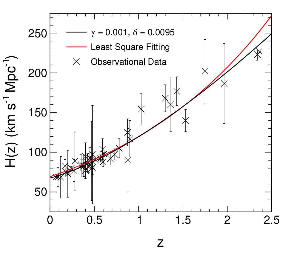
Further, to get the precise values of above free parameters for both the cases, which should be consistent with the $\Lambda$ CDM model at least around the present epoch, we have considered the compilation of 43 observational Hubble parameter data against 43 different values of redshift Akarsu_2019; Gogoi_2021 as shown in Table 1. We have plotted the best fitted curve to this set of Hubble parameter data against the redshift by using a non-linear curve fitting (least square fitting) technique as shown in Fig. 3. From the curve we have calculated the value of $\alpha\beta=0.86275$ for the case I at $z=0$ . It is important to mention that we may be able to consider a set of values of $\alpha$ and $\beta$ , which satisfy the condition that $\alpha\beta=0.86275$ . Thus, we can use different sets of $\alpha$ and $\beta$ with this condition. Here, we have not consider any special set of values of $\alpha$ and $\beta$ , but just considered the condition $\alpha\beta=0.86275$ in the rest of the paper. However, it is not easy to get the values of the parameters $\delta$ and $\gamma$ for the case II using this method. So, for the case II we have used a suitable set of values of $\delta$ and $\gamma$ , for which the expression of $H(z)$ for this case (Eq. (70)) gives a curve very close to the least square fitting curve to the observational data as shown in Fig. 3. This set of values of $\delta$ and $\gamma$ are found to be 0.001 and 0.0095 respectively, which is the same as the lower limit values of these parameters found from the analysis with Fig. 2. Thus the graphical plots of $H(z)$ for both the cases obtained from these derived free parameters values as mentioned above should be consistent with the $\Lambda$ CDM plot shown in Fig. 2, especially for the range of small $z$ .

Table 1: Presently available observational Hubble parameter (

H^{obs}(z)

) data set.

H^{obs}(z)

is in unit of km/s/Mpc.

$z$	$H^{obs}(z)$	Reference	$z$	$H^{obs}(z)$	Reference
0.0708	69.0 $\pm$ 19.68	Zhang_2014	0.48	97.0 $\pm$ 62.0	Ratsimbazafy_2017
0.09	69.0 $\pm$ 12.0	Simon_2005	0.51	90.8 $\pm$ 1.9	Alam_2017
0.12	68.6 $\pm$ 26.2	Zhang_2014	0.57	92.4 $\pm$ 4.5	Samushia_2013
0.17	83.0 $\pm$ 8.0	Simon_2005	0.593	104.0 $\pm$ 13.0	Moresco_2012
0.179	75.0 $\pm$ 4.0	Moresco_2012	0.60	87.9 $\pm$ 6.1	Blake_2012
0.199	75.0 $\pm$ 5.0	Moresco_2012	0.61	97.8 $\pm$ 2.1	Alam_2017
0.20	72.9 $\pm$ 29.6	Zhang_2014	0.68	92.0 $\pm$ 8.0	Moresco_2012
0.24	79.69 $\pm$ 2.65	Gaztanaga_2009	0.73	97.3 $\pm$ 7.0	Blake_2012
0.27	77.0 $\pm$ 14.0	Simon_2005	0.781	105.0 $\pm$ 12.0	Moresco_2012
0.28	88.8 $\pm$ 36.6	Zhang_2014	0.875	125.0 $\pm$ 17.0	Moresco_2012
0.35	84.4 $\pm$ 7.0	Xu_2013	0.88	90.0 $\pm$ 40.0	Ratsimbazafy_2017
0.352	83.0 $\pm$ 14.0	Moresco_2012	0.90	117.0 $\pm$ 23.0	Simon_2005
0.38	81.9 $\pm$ 1.9	Alam_2017	1.037	154.0 $\pm$ 20.0	Moresco_2012
0.3802	83.0 $\pm$ 13.5	Moresco_2016	1.30	168.0 $\pm$ 17.0	Simon_2005
0.40	95.0 $\pm$ 17.0	Simon_2005	1.363	160.0 $\pm$ 33.6	Moresco_2015
0.4004	77.0 $\pm$ 10.2	Moresco_2016	1.43	177.0 $\pm$ 18.0	Simon_2005
0.4247	87.1 $\pm$ 11.2	Moresco_2016	1.53	140.0 $\pm$ 14.0	Simon_2005
0.43	86.45 $\pm$ 3.68	Gaztanaga_2009	1.75	202.0 $\pm$ 40.0	Simon_2005
0.44	82.6 $\pm$ 7.8	Blake_2012	1.965	186.5 $\pm$ 50.4	Moresco_2015
0.4497	92.8 $\pm$ 12.9	Moresco_2016	2.34	223.0 $\pm$ 7.0	Delubac_2015
0.47	89.0 $\pm$ 50.0	Ratsimbazafy_2017	2.36	227.0 $\pm$ 8.0	Ribera_2014
0.4783	80.9 $\pm$ 9.0	Moresco_2016

IV.0.2 Ricci scalar

Ricci scalar is an important parameter to specify the geometric property of spacetime of the universe. Some mathematical and graphical analysis of the evolution of Ricci scalar for various cosmological models in modified cosmology are also found in Ref. Gogoi_2021. So, to understand the evolution of Ricci scalar in our anisotropic model of the universe, we have plotted Ricci scalar $R(z)$ against the redshift ( $z$ ) for the case I and case II by using Eqs. (48) and (75) respectively as shown in Fig. 4. In this plot we have used the observationally constrained value of $\alpha\beta=0.86275$ for the case I, and $\gamma=0.001$ and $\delta=0.0095$ for the case II as mentioned in the previous subsection. Here, we have also shown the plot of this cosmological parameter for the $\Lambda$ CDM model. Figure shows that both the cases of our model are consistent with the $\Lambda$ CDM model from the present epoch to the near past. However, the deviation of both the cases increases with higher curvature of spacetime for the case I and with lower curvature for the case II, from the $\Lambda$ CDM model as we move towards the distant past.

IV.0.3 Deceleration Parameter and Equation of State

As the deceleration parameter $q(z)$ is an important parameter to understand the pattern of evolution of the universe, we have plotted it with respect to $1+z$ for the both the cases of our model for the constrained values of the free parameters as mentioned above by using Eqs. (46) and (73) along with the plot for the $\Lambda$ CDM model as shown in Fig. 5. It is found that for both the cases, at $z$ = 0, $q(0)$ tends to $-0.55$ , which is a good agreement with the $\Lambda$ CDM model’s prediction for the current value of $q(z)$ . In reality for any value of $z$ , $q(z)$ for both the cases shows a good agreement with the $\Lambda$ CDM model, especially the case II has the excellent agreement. This implies that the pattern of evolution of our anisotropic model of universe is same as that of the isotropic model.

Similarly, the Equation of State (EoS) is an important cosmological parameter to understand the composition of the universe as well as its characteristics. We have plotted the EoS ( $\omega$ ) against $1+z$ for both the cases by using Eq. (47) and (74) with the constrained values of free model parameters as shown in Fig. 6. We found that at $z=0$ , EoS $\omega$ is close to $-0.7$ for both the cases, which is also consistent with the $\Lambda$ CDM model and agrees with the current era of the universe as the dark energy era. The curves show good agreement with the $\Lambda$ CDM model (in fact it is excellent for the case II) and hence support the three phases of the universe, viz., the radiation dominated phase ( $\omega=1/3$ ), the matter dominated phase ( $\omega=0$ ) and the dark energy phase ( $\omega=-1$ ). Thus this anisotropic model of the universe has the same evolution characteristics as the isotropic model of the universe.

IV.0.4 Distance modulus

The distance modulus is a reliable observational parameter to understand the cosmic evolution with redshift. Here, we have plotted the distance modulus ( $D_{m}$ ) against redshift for both the cases with the free model parameters as mention above by using Eqs. (49) and (76) in Eq. (27) along with the Union2.1 observational data Suzuki_2012 and $D_{m}$ for the $\Lambda$ CDM model as shown in Fig. 7. It is clear from the figure that for both the cases, for the constrained free parameter values, the distance modulus plot shows excellent agreement with observational data along with the $\Lambda$ CDM plot. This implies that the anisotropic model of the universe agrees very well with the observed data of the distance modulus of galaxies.

IV.0.5 Anisotropy density parameter

The anisotropy density parameter is an important parameter to understand the possible anisotropy that exists in the universe. For the case I it’s value is zero, but for the case II it has a definite expression as mentioned in Eq. (77). Fig. 8 shows the plot of this $\Omega_{\sigma}$ against $1+z$ for the constrained values of $\delta$ and $\gamma$ . This figure suggests that a considerable amount of anisotropy exists for a much higher value of redshift, which indicates that the universe had prominent anisotropic character in its early stages and which is now almost reduced to zero. The existence of anisotropy after inflation period can be explained with the idea like breaking the Lorentz invariance by introducing a condensation of vector field Kanno_2008, slow roll phase of vector fields like as inflation field in chaotic inflationary scenario, Golovnev_2008; Kanno_2008; Watanabe_2009 or considering anisotropic inflation model with vector impurityKanno_2008 etc. However, this is a broad area of study and hence to be considered latter. In Ref. Akarsu_2019, the upper limits of the present value of the anisotropy density parameter ( $\Omega_{\sigma 0}$ ) has been calculated by using the BAO and CMB data for the matter dominated recombination era as $\Omega_{\sigma 0}\leq 10^{-15}$ , and by demanding that the standard big bang nucleosynthesis (BBN) is not significantly affected by the expansion anisotropy as $\Omega_{\sigma 0}\leq 10^{-23}$ . From these two upper limits of $\Omega_{\sigma 0}$ we have calculated the corresponding values of the free parameters $\delta$ and $\gamma$ of the case II, and found that their values may lie in between $10^{-3}$ and $10^{-8}$ . It should be noted that this calculated upper limit of values of $\delta$ and $\gamma$ is in agreement with their constrained values obtained from the Hubble parameter data as mentioned above.

IV.0.6 Relative shear anisotropy parameter

The relative shear anisotropy parameters $r$ and $s$ can be defined as Barrow_1997

r=\frac{H_{1}-H_{2}}{H},\;\;s=\frac{H_{1}-H_{3}}{H},

where as mentioned above $H_{1},H_{2},H_{3}$ are the directional Hubble parameters and $H$ is the average Hubble parameter. The parameters $r$ and $s$ provide the information about if the anisotropy exists in different directions and their plot against redshift gives the picture about the evolution of directional anisotropy. Fig. 9 shows the plots of both the parameters for case II. The figure shows that there was a considerable amount of relative shear anisotropy present for the higher value of redshift $(z)$ . Thus the model predicts the existence of higher value of relative shear anisotropy in the early stage of the universe. However, for the case I both these parameters vanish. Thus for case I, the universe has no relative shear anisotropy.

IV.0.7 Density parameter of matter

To visualize how the matter density parameter varies from early stages to present epoch according to our anisotropic model of the universe, we have plotted the $\Omega_{m}/\Omega_{mo}$ against the redshift in Fig. 10 by using Eq. (50) and (78) for the case I and case II respectively for the constrained values of free parameters for each cases. The left panel of Fig. 10 is for case I and the right panel is for case II. We have plotted this parameter for both the cases against the value of $z$ up to $10^{6}$ . From the figure, we have seen that there is a matter dominated era up to $z$ $\sim 10^{3}$ for both the cases and it supports the matter dominated region $0.5\leq z\leq 3000$ as mentioned in Ref. Frieman_2008. For very high values of $z$ , the density parameter for matter drops down considerably close to zero. It suggests that the universe was radiation dominated at it’s early stage. Thus this anisotropic model of the universe agrees well with the observed or predicted evolution nature of the standard cosmology. However, there are differences between the matter density parameter evolution in case I and case II. Firstly, falling of this parameter for very high $z$ values is not smooth in the case II in comparison to in the case I. Secondly, in the case I the ratio $\Omega_{m}/\Omega_{mo}$ moves gradually towards one as $z$ tends to zero as expected, but in the case II this ratio reached to the value one before $z$ reached its zero value.

IV.0.8 Age of the universe

According to the standard model of cosmology ( $\Lambda$ CDM) the age of the universe is calculated to be $\sim$ 13.786 Gyr. To find the age of the universe in our model we have calculated it by using Eqs. (45) and (72) for the case I and case II respectively with the constrained sets of corresponding free parameters. We found that according to case I the age of the universe is $\sim$ 13.084 Gyr and according to case II it is $\sim$ 13.741 Gyr. Thus we see that case II result agrees very well with the results of the standard model of cosmology with a deviation of only 0.33%. Whereas the deviation of the result in case I is 5.09%.

V Conclusions

In this study we have considered the simplest Bianchi type I metric with slight modifications in directional scale factors for two different cases to understand the possible anisotropy that may exist in the universe. Here, we have used the generalized equations of Bianchi type I cosmological model and implemented them in both the considered cases. Starting from the field equations, we have construct all the cosmological parameters including average Hubble parameter, luminosity distance, distance modulus, deceleration parameter, equation of state, shear scalar and various density parameters etc. for both the cases. After the mathematical constructions, we have tried to plot various parameters with respect to cosmological redshift and compare the results with $\Lambda$ CDM model which is the best fitted model to cosmological data till date. Also we compare the results with various observational data like HKP data, SVJ05 data, SJVKS10 data and GCH09 data for the Hubble parameter and with Union 2.1 data for the distance modulus. Further, we have used observational data of Hubble parameter given in Table 1 that are obtained from various sources as mentioned in the table to constrained the free parameters of both the cases i.e. $\alpha$ and $\beta$ for the case I, and $\delta$ and $\gamma$ for the case II as shown in Fig.3. In this context, explicitly we should state that we have used the observational Hubble parameter data to find out the best possible values of model parameters as mentioned above. For the case I, we have equated Eq. (43) with $H_{0}$ for $z=0$ using the Planck $2018$ data Planck_2018 for the same and found that $\alpha\beta=0.86275$ . Thus any set of values of $\alpha$ and $\beta$ which satisfies this condition are eligible for consideration in the case I. In our work, we have not considered any special set of values of $\alpha$ and $\beta$ but taken the condition as a whole for the graphical analysis. However, for case II this method is not suitable as the expression for the Hubble parameter in this case is complicated as compared to the case I. Therefore we have fitted the 43 observational Hubble parameter data in Table 1 using the least square fitting technique. Then we have changes our model parameters $\delta$ and $\gamma$ in Eq. (70) for $H(z)$ of the case II to find out which values of these parameters give the suitable or close result with the least square fitting curve. In our analysis we have found that for $\delta=0.001$ and $\gamma=0.0095$ , the plot of the Hubble parameter fairly agrees with the fitting curve as shown in Fig. 3. Thus from our analysis we have taken $\alpha\beta=0.86275$ for the case I, and $\delta=0.001$ , $\gamma=0.0095$ for the case II as the constrained values of the model parameters in all other graphical analysis.

After constraining the model parameters we have plotted various cosmological parameters against cosmological redshift for both the cases with the constrained values of free parameters and tried to explain those plots. From the results of this analysis we have found that for the case I, where the directional scale factors are modified by multiplicative constants, the model unable to show any kind of anisotropy as the shear scalars and density parameter of anisotropy are zero in this case. It is to be noted that for $\alpha=\beta=1$ , the case I is reduced to the $\Lambda$ CDM model. For the case II, we found relatively higher amount of anisotropy as compared to case I for higher values of redshift and it becomes very very small at $z\leq$ $20$ (see Fig. 8). The case II also shows the presence of relative shear anisotropy, which is obviously very small for small value of redshift. The case II also reduces to the $\Lambda$ CDM model when $\delta=\gamma=0$ . Moreover, in terms of age of the universe the case II is found to be in very good agreement with the $\Lambda$ CDM model. Further, we have found that the current value of the Hubble parameter ( $H_{0}$ ) for the case I is $69.31$ and for the case II is $67.56$ . The result obtained for case II shows more consistency with the Planck 2018 result Planck_2018. Similarly, the current value of deceleration parameter for case I is $-0.47$ and for case II is $-0.54$ . Here also the result obtained from case II is more consistent with the Planck $2018$ data Planck_2018. Furthermore, the constrained values of model parameters for both the cases give the matter dominated region in the density parameter of matter vs redshift ( $z$ ) plots of Fig. 10, which show good agreement within the range $0.5\leq z\leq 3000$ as mentioned in Ref. Frieman_2008. For the range of values of density parameters of anisotropy $\Omega_{\sigma 0}$ as suggested in Ref. Akarsu_2019 i.e. $10^{-23}\leq\Omega_{\sigma 0}\leq 10^{-15}$ , the values of $\delta$ and $\gamma$ lies in between $10^{-8}$ and $10^{-3}$ for the case II.

Thus from our work, we have shown that even there exist variations in directional scale factors, the Bianchi type I model sometime gives purely isotropic universe just like the case I. Also we have found that although very small variations of directional scale factors unable to change the isotropic nature of the universe significantly in the current state, but it may possess relatively higher contribution of anisotropy in early stage of the universe compared to the current state.

Finally, it needs to be mentioned that in most of the past studies on various anisotropic cosmological models authors tried to constraint the cosmological parameters related to the possible anisotropy of the universe using the available cosmological data with various statistical methods. For example, in Refs. Akarsu_2019; Andrade_2018 Bayesian inference technique is used, goodness of fit is used in Refs. Bunn_1996 and simulation techniques like Monte Carlo is used in Refs. Hansen_2004; Bunn_1996. Whereas in our work we constrain our model parameters using the available cosmological data as well as the constrained anisotropic density parameter to predict the possible anisotropy present in the universe as mentioned above. Apart from this difference, our work is mainly based on analytical techniques in contrast to statistical methods of previous studies as mentioned. We have derived analytical expressions of all the cosmological parameters based on our model, that contain the anisotropic parameters of the model. So these cosmological parameters and hence our findings can hopefully be tested with the early universe cosmological data that may be available in future from the future advanced telescopes, such as the Thirty Meter Telescope TMT, Extremely Large Telescope ELT, CTA CTA etc.

References

(1) L.Tedesco, Eur. Phys. J. Plus 133, 188 (2018) [arXiv:1804.11203].
(2) J. Colin, R. Mohayaee, M. Rameez and S. Sarkar, A & A 631, L13 (2019) [arXiv:1808.04597].
(3) P. J. E. Peebles, Principles of Physical Cosmology (Princeton University Press) (1994).
(4) K. Bamba, S. Capozziello, S. Nojiri and S. D. Odintsov, Astrophysics and Space Science 342, 155 (2012) [arXiv:1205.3421].
(5) C. Ma and T.-J. Zhang, ApJ 730 74 (2011) [arXiv:1007.3787].
(6) H. Hossienkhani, N. Azimi, S. Gheysari and Z. Zarei, New Astronomy 84, 101465 (2021).
(7) Ö. Akarsu, S. Kumar, S. Sharma, and L. Tedesco, Phys. Rev. D 100, 023532 (2019) [arXiv:1905.06949].
(8) L. Campanelli, P. Cea, G. L. Fogli and A. Marrone, Phys Rev. D 83, 103503 (2011) [arXiv:1711.05974].
(9) D. C. Maurya, Int. J. Geom. Methods Mod. Phys. 15, 1850019 (2018).
(10) E. F. Bunn, P. G. Ferreira and J. Silk, Phys. Rev. Lett. 77, 2883 (1996) [arXiv:astro-ph/9605123].
(11) A. de Oliveira-Costa, M. Tegmark, M. Zaldarriaga and A. Hamilton, Phys. Rev. D 69, 063516 (2004) [arXiv:astro-ph/0307282].
(12) C. J. Copi, D. Huterer, G.D. Starkman, Phys. Rev. D 70, 043515 (2004) [arXiv:astro-ph/0310511].
(13) H. K. Eriksen et al., APJ 605, 14 (2004) [arXiv:astro-ph/0307507].
(14) H. K. Eriksen et al., APJ 609, 1198 (2004).
(15) P. Cea, arXiv:2201.04548.
(16) L. Perivolaropoulos, Galaxies 2(1), 22-61 (2014) [arXiv:1401.5044].
(17) J. A. Frieman, M. S. Turner and D. Huterer, Annu. Rev. A & A 46, 385–432 (2008) [arXiv:0803.0982].
(18) A. Berera, R.V. Buniy, and T.W. Kephart, JCAP 10, (2004) 016. [arXiv:hep-ph/0311233]
(19) R. V. Buniy, A. Berera, and T.W. Kephart, Phys. Rev. D 73, 063529 (2006) [arXiv:hep-th/0511115].
(20) L. Campanelli, P. Cea, L. Tedesco, Phys. Rev. Lett. 97, 131302 (2006) [arXiv:astro-ph/0606266].
(21) L. Campanelli, P. Cea, L. Tedesco, Phys. Rev. D 76, 063007 (2007) [arXiv:0706.3802].
(22) F. K. Hansen, A. J. Banday, K. M. Gorski, MNRAS 354, 641 (2004) [arXiv:astro-ph/0404206].
(23) P. Vielva et al., APJ 609, 22 (2004)
(24) H. Hossienkhani, H. Yousefi and N. Azimi, Int. J. Geom. Methods Mod. Phys. 15 1850200 (2018).
(25) S. Nojiri, S. D. Odintsov, and V. K. Oikonomou, Phys. Rept. 692, 1 (2017) [arXiv:1705.11098].
(26) D. J. Gogoi and U. D. Goswami, Int. J. Mod. Phys. D 31, 2250048 (2022) [arXiv:2108.01409].
(27) N. Parbin and U. D. Goswami, Mod. Phys. Lett. A 36, 2150265 (2021) [arXiv:2007.07480].
(28) D . W. Hogg et al., ApJ 624, 54 (2005) [arXiv:astro-ph/0411197].
(29) M. I. Scrimgeour,MNRAS 425, 116 (2012) [arXiv:1205.6812].
(30) Y. Y. Wang and F. Y. Wang, MNRAS 474, 3516–3522 (2018).
(31) H. K. Eriksen et al., arXiv:astro-ph/0701089.
(32) J. Hoftuft et al., APJ 699, 985–989, (2009).
(33) F. Paci et al., MNRAS 407, 399 (2010).
(34) A. Mariano and L. Perivolaropoulos, Phys. Rev. D 87, 043511 (2013) [arXiv:1211.5915].
(35) W. Zhao and L. Santos, arXiv:1604.05484v3.
(36) I. Antoniou and L. Perivolaropoulos, JCAP 12, 012 (2010) [arXiv:1007.4347].
(37) A. Mariano and L. Perivolaropoulos,Phys. Rev. D 86, 083517 (2012) [arXiv:1206.4055].
(38) J. S. Wang and F.Y. Wang, MNRAS 443 1680–1687 (2014).
(39) A. Kashlinsky, F. Atrio-Barandela, D. Kocevski, and H. Ebeling, Apj 686, L49 (2008) [arXiv:0809.3734].
(40) R. Watkins, H. A. Feldman and M. J. Hudson, MNRAS 392, 743–756 (2009).
(41) H. A. Feldman, R. Watkins and M. J. Hudson, MNRAS 407, 2328 (2010).
(42) A. Kashlinsky et al., ApJ 712, L81 (2010) [arXiv:0910.4958].
(43) G. Lavaux, R. B. Tully, R. Mohayaee, and S. Colombi, ApJ 709, 483 (2010).
(44) A. Moss, D. Scott, J. P. Zibin and R. Battye, Phys. Rev. D 84, 023014 (2011) [arXiv:1011.2990].
(45) J. K. Webb et al., Phys. Rev. Lett. 107, 191101 (2011) [arXiv:1008.3907].
(46) J. A. King et al., MNRAS 422, 3370 (2012).
(47) A. M. M. Pinho and J. A. P. Martins, Phys. Lett. B. 756, 121 (2016) [arXiv:1603.04498].
(48) N. Aghanim et al. (Planck Collaboration), A&A 641, A6 (2020) [arXiv:1807.06209].
(49) B. C. Paul and D. Paul, Pramana J. Phys. 71, 6 (2008).
(50) J. D. Barrow, Phys Rev. D. 55, 7451 (1997)[arXiv:gr-qc/9701038].
(51) E. J. Copeland , M. Sami and S. Tsujikawa, Int. J. Mod. Phys. D 15,1753-1935 (2006) [arXiv:hep-th/0603057v3].
(52) T. Delubac et al., A & A 574, A59 (2015) [arXiv:1404.1801].
(53) C. Zhang et al., Res. Astron. Astrophys 14, 1221 (2014) [arXiv:1207.4541].
(54) A. F. Ribera et al., JCAP 05, 027 (2014) [arXiv:1311.1767].
(55) J. Simon et al., Phys. Rev. D 71, 123001 (2005) [arXiv:astro-ph/0412269].
(56) M. Moresco et al., JCAP 05, 014 (2016) [arXiv:1601.01701].
(57) A. L. Ratsimbazafy et al., MNRAS 4673239 (2017).
(58) M. Moresco, MNRAS 450, L16–L20 (2015).
(59) M. Moresco et al., JCAP 08, 006 (2012) [arXiv:1201.3609].
(60) S. Alam et al., MNRAS 470, 2617 (2017).
(61) J. Simon, L. Verde and R. Jimenez, Phys. Rev. D 71 123001 (2005) [arXiv:astro-ph/0412269].
(62) D. Stern et al., JCAP 02, 008 (2010) [arXiv:0907.3149].
(63) E. Gaztañaga, A. Cabré and L. Hui, MNRAS 399, 1663 (2009).
(64) N. Suzuki et al., ApJ 746, 85 (2012) [arXiv:1105.3470].
(65) X. Xu et al. MNRAS 431, 2834 (2013) [arXiv:1206.6732].
(66) L. Samushia et al., MNRAS 429, 1514 (2013) [arXiv:1206.5309v2].
(67) C. Blake et al., MNRAS 425, 405 (2012) [arXiv:1204.3674].
(68) S. Kanno, M. Kimura, J. Soda and S. Yokoyama, JCAP 08, 034 (2008) [arXiv:0806.2422]
(69) A. Golovnev, V. Mukhanov and V. Vanchurin, JCAP 06, 009 (2008) [arXiv:0802.2068]
(70) M. Watanabe, S. Kanno and J. Soda, Phys.Rev.Lett. 102,191302 (2009) [arXiv:0902.2833 ]
(71) U. Andrade, C. A. P. Bengaly, J. S. Alcaniz and B. Santos, Phys. Rev. D 97, 083518 (2018) [arXiv:1711.10536 ]
(72) Thirty Meter Telescope, www.tmt.org
(73) Extremely Large Telescope, https://elt.eso.org
(74) Cherenkov Telescope Array, www.cta-observatory.org