\midlauthor

¹ Department of Pathology and Molecular Pathology, University Hospital, University of Zurich, Switzerland.
² Department of Pathology, University of Bern, Switzerland.
³ Department of Mathematics, City University of Hong Kong, China.
⁴ Department of Oncology and Nuffield Department of Medicine, University of Oxford, UK.

Towards IID representation learning and its application on biomedical data

Jiqing Wu¹ Email: jiqing.wu@usz.ch Inti Zlobec² Email: inti.zlobec@pathology.unibe.ch Maxime Lafarge¹ Email: maxime.lafarge@usz.ch Yukun He³ Email: yukunhe@cityu.edu.hk Viktor H. Koelzer^1,4 Email: viktor.koelzer@usz.ch Affiliation: Affiliation: Affiliation: Affiliation:

Abstract

Due to the heterogeneity of real-world data, the widely accepted independent and identically distributed (IID) assumption has been criticized in recent studies on causality. In this paper, we argue that instead of being a questionable assumption, IID is a fundamental task-relevant property that needs to be learned. Consider $k$ independent random vectors $\mathsf{X}^{i=1,\ldots,k}$ , we elaborate on how a variety of different causal questions can be reformulated to learning a task-relevant function $\phi$ that induces IID among $\mathsf{Z}^{i}\mathrel{\vbox{\hbox{.}\hbox{.}}}=\phi\circ\mathsf{X}^{i}$ , which we term IID representation learning.

For proof of concept, we examine the IID representation learning on Out-of-Distribution (OOD) generalization tasks. Concretely, by utilizing the representation obtained via the learned function that induces IID, we conduct prediction of molecular characteristics (molecular prediction) on two biomedical datasets with real-world distribution shifts introduced by a) preanalytical variation and b) sampling protocol. To enable reproducibility and for comparison to the state-of-the-art (SOTA) methods, this is done by following the OOD benchmarking guidelines recommended from WILDS. Compared to the SOTA baselines supported in WILDS, the results confirm the superior performance of IID representation learning on OOD tasks. The code is publicly accessible via https://github.com/CTPLab/IID_representation_learning.

^†^†year: 2022^†^†workshop: MIDL 2022 – Full Paper track

keywords

IID, IID representation learning, OOD generalization, causality, biomedical.

1 Introduction

In machine learning (Vapnik 1999), we commonly assume that data entries ${(y_{i},\bm{x}_{i})}_{i=1,\ldots,n}$ are independently drawn from the same probability distribution $\mathbb{P}_{(\mathsf{Y},\bm{\mathsf{X}})}$ of a random vector $(\mathsf{Y},\bm{\mathsf{X}})$ . This is referred to as the independent and identically distributed (IID) assumption. However, real-world data is usually characterized by significant heterogeneity (Bareinboim 2014; Peters et al. 2017; Arjovsky et al. 2019; Rosenfeld et al. 2021). Controlling data heterogeneity is particularly critical in application of data driven methods to the medical domain (Cios and Moore 2002), as medical algorithms that suffer from prediction degradation on heterogeneous cohorts can have severe consequences in medical practice. Consequently, the IID assumption needs to be critically questioned.

The task of learning a robust model that is resistant to a heterogeneous data distribution is formally denoted as Out-of-Distribution generalization (OOD) (Arjovsky et al. 2019; Koh et al. 2021). For a thorough overview we refer interested readers to (Shen et al. 2021). A large number of studies with diverse methodologies (Peters et al. 2016; Ganin et al. 2016; Sun and Saenko 2016; Rojas-Carulla et al. 2018; Arjovsky et al. 2019; Sagawa et al. 2020; Rosenfeld et al. 2021) have been proposed to address this issue. From the viewpoint of domain adaptation (Pan et al. 2010), the root causes of OOD failure come from domain or task shift (Wang and Deng 2018). There have been many studies dedicated to resolve the challenge. (Sun et al. 2016; Sun and Saenko 2016) proposed to align the second-order statistics of the source and target distributions. In case of simultaneous domain and task shift, (Gong et al. 2016) suggested to pinpoint conditional transferable components. Further, (Long et al. 2018) reduced the shifts in the data distributions across domains via adversarial learning (Goodfellow et al. 2014). Built upon the invariant property reflected in causality (Pearl et al. 2000), (Peters et al. 2016) firstly proposed the seminal invariant causal prediction (ICP) framework. Later, (Rojas-Carulla et al. 2018) investigated the invariant set and extended the ICP to transfer learning (Pan and Yang 2009; Muandet et al. 2013; Zhuang et al. 2020). Motivated by the ICP, invariant risk minimization (IRM) (Arjovsky et al. 2019) was subsequently proposed to learn an invariant predictor that is optimal for all environments. Recently, (Schölkopf et al. 2021) pointed out the essential role of causal representation learning in OOD generalization. In a nutshell, (Schölkopf et al. 2021) argued that cause-effect relations are critical components of reasoning chains that remain robust in situations beyond training tasks. However, causal variables are usually not given in machine learning tasks. Thus, (Schölkopf et al. 2021) suggested learning causal representations to resolve the limitation of current approaches for OOD generalization.

Inspired by impactful studies centered on the investigation of statistical invariance:

•

We introduce a novel pair of definitions: IID symmetry and its generalization. These definitions reflect the core message delivered in the work, i.e., instead of being a questionable assumption, IID is a fundamental task-relevant property that needs to be learned.
•

Then, we systematically discuss how IID and causality are two sides to the same coin. Consider $k$ independent random vectors $\mathsf{X}^{i=1,\ldots,k}$ , we elaborate concrete examples of reformulating diverse causal problems to learning a task-relevant function $\phi$ that induces IID among $\mathsf{Z}^{i}\mathrel{\vbox{\hbox{.}\hbox{.}}}=\phi\circ\mathsf{X}^{i}$ , which we term IID representation learning.
•

For proof of concept, we examine the IID representation learning on Out-of-Distribution (OOD) generalization tasks. Concretely, in utilizing the representation obtained via the learned function that induces IID, we conduct molecular prediction experiments on two comprehensive biomedical datasets (RxRx1 (Taylor et al. 2019) and Swiss Colorectal Cancer (SCRC) (Nguyen et al. 2021)). By following the OOD benchmarking guidelines recommended from WILDS (Koh et al. 2021), we demonstrate that the IID representation learning can improve the molecular predictions compared to the SOTA baselines supported in WILDS.

2 Proposed Definition

As elaborated above, the common ground of causal studies usually starts with exploring statistical invariance. Thus, we introduce the definitions of IID symmetry and its generalization as follows: Consider $k+n$ independent random vectors $\mathsf{X}^{1},\ldots,\mathsf{X}^{k},\mathsf{X}^{k+1},\ldots,\mathsf{X}^{k+n}$ and a Lebesgue integrable $\phi:\mathbb{R}^{l+1}\mapsto\mathbb{R}^{m+1}$ , for $i=1,\ldots,k+n$ , let $\mathbb{Q}_{\mathsf{X}^{i}}$ be a query distribution¹¹ 1 i.e., a probability measure induced by $\mathsf{X}^{i}$ (e.g., conditional, marginal, and probability distribution of $\mathsf{X}^{i}$ ) that is relevant to the question of interest. of $\mathsf{X}^{i}=(\mathsf{x}_{0}^{i},\mathsf{x}_{1}^{i},\ldots,\mathsf{x}_{l}^{i})$ , let $\mathsf{Z}^{i}=(\mathsf{z}_{0}^{i},\mathsf{z}_{1}^{i},\ldots,\mathsf{z}_{m}^{i})\mathrel{\vbox{\hbox{.}\hbox{.}}}=\phi\circ\mathsf{X}^{i}$ and $\mathbb{Q}_{\mathsf{Z}^{i}}\mathrel{\vbox{\hbox{.}\hbox{.}}}=\mathbb{Q}_{\mathsf{X}^{i}}\circ\phi^{-1}$ ,

Definition 1.

We say that $\mathsf{X}^{1},\ldots,\mathsf{X}^{k}$ have an ( $\phi-$ )IID symmetry if $\phi$ induced $\mathbb{Q}_{\mathsf{Z}^{1}},\ldots,\mathbb{Q}_{\mathsf{Z}^{k}}$ are identical distributions, i.e., $\mathbb{Q}_{\mathsf{Z}^{1}}=\ldots=\mathbb{Q}_{\mathsf{Z}^{k}}$ . Further, we say that the ( $\phi-$ )IID symmetry is generalizable to $\mathsf{X}^{k+1},\ldots,\mathsf{X}^{k+n}$ if $\mathbb{Q}_{\mathsf{Z}^{1}},\ldots,\mathbb{Q}_{\mathsf{Z}^{k}},\mathbb{Q}_{\mathsf{Z}^{k+1}},\ldots,\mathbb{Q}_{\mathsf{Z}^{k+n}}$ are identical distributions.

Remark 1.

It is not difficult to see that $\mathsf{Z}^{1},\ldots,\mathsf{Z}^{k+n}$ are independent, since w.l.o.g. we can reduce the proof to the simpler case of two random vectors $\mathsf{Z}^{1},\mathsf{Z}^{2}$ and $\phi$ being continuous. Let $f:\mathbb{R}^{m+1}\to\mathbb{R}$ be bounded and continuous, then $f\circ\phi:\mathbb{R}^{l+1}\to\mathbb{R}$ is also bounded and continuous. We have

	$\displaystyle\mathbb{E}[f(\mathsf{Z}^{1})f(\mathsf{Z}^{2})]$	$\displaystyle=\mathbb{E}[(f\circ\phi)(\mathsf{X}^{1})(f\circ\phi)(\mathsf{X}^{2})]=\mathbb{E}[f\circ\phi(\mathsf{X}^{1})]\mathbb{E}[f\circ\phi(\mathsf{X}^{2})]$		(1)
		$\displaystyle=\mathbb{E}[f(\mathsf{Z}^{1})]\mathbb{E}[f\mathsf{Z}^{2})],$		(1)

where the second equality comes from the independence of $\mathsf{X}^{1}$ and $\mathsf{X}^{2}$ . As a large class of functions including piece-wise continuous function (neural network) satisfies the Lebesgue integrability condition, we claim the map $\phi$ discussed in this paper always induces independence. Since for $i=1,\ldots,k+n$ , $\mathsf{Z}^{i}$ is independent and identically distributed w.r.t. $\mathbb{Q}_{\phi\circ\mathsf{X}^{i}}$ , we call $\mathsf{Z}^{i}$ an ( $\phi-$ )IID representation. It is worth mentioning that the entries of $\mathsf{Z}^{i}$ are not required to be independent.

Remark 2.

For $i=1,\ldots,k+n$ , if $\mathbb{Q}_{\mathsf{X}^{i}}=\mathbb{P}_{\mathsf{X}^{i}}$ is the probability distribution of $\mathsf{X}^{i}$ , then $\mathsf{Z}^{1},\ldots,\mathsf{Z}^{k+n}$ are IID in the canonical sense according to Rem. 1. Besides, the trivial IID symmetry and its generalization always exist, for instance we can define a trivial $\phi$ such that $\phi\circ\mathsf{X}^{i}=\text{const}$ .

3 From Causality to IID

Causal inference is a fundamental research domain that reflects the zeitgeist in machine learning (Luo et al. 2020). Broadly speaking, prior studies on causal inference can be categorized into two areas of research: causal identification (Pearl et al. 2009; Peters et al. 2017; Hernán and Robins 2020) and causal transportation (Balke and Pearl 1995; Bareinboim and Pearl 2014; Bareinboim 2014). The former aims to either identify the underlying Structural Causal Models (SCM) (Peters et al. 2017) or quantify the Average Causal Effect (ACE) (Hernán and Robins 2020), whereas the latter is often meant for licensing the transportable causal knowledge from one population to another (Bareinboim and Pearl 2014; Bareinboim 2014). In a recent study (Schölkopf et al. 2021), the authors propose causal representation learning to resolve OOD generalization. To link causal inference and IID, we first introduce two prerequisite concepts:

Structural Causal Model. Following the specification in (Peters et al. 2016; Peters et al. 2017), consider a Structural Causal model (SCM), i.e., there exists a random vector $\mathsf{X}=(\mathsf{x}_{0},\ldots,\mathsf{x}_{l})$ and a directed acyclic graphs (DAG) consisting of vertices $\mathsf{x}_{0},\ldots,\mathsf{x}_{l}$ and $\delta_{0},\ldots,\delta_{l}$ such that for $j=0,\ldots,l$ we have

\mathsf{x}_{j}=f_{j}(\mathsf{X_{PA_{j}}},\delta_{j}),\delta_{j}\Perp\mathsf{X_{PA_{j}}},

(2)

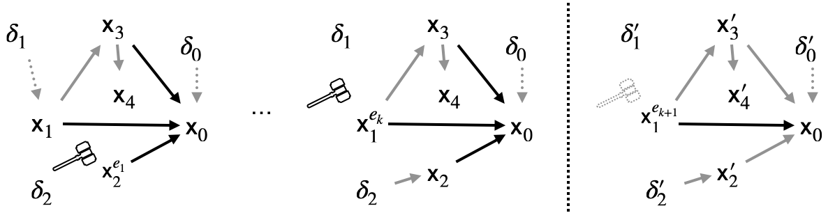
where $\mathsf{X_{PA_{j}}}\subset\{\mathsf{x}_{0},\mathsf{x}_{1},\ldots,\mathsf{x}_{l}\}$ is the set of known parents of $\mathsf{x}_{j}$ , $\delta_{j}$ is the unknown (parent) noise. By drawing arrow(s) from $\mathsf{X_{PA_{j}}},\delta_{j}$ to $\mathsf{x}_{j}$ defined in Eq. 2, we obtain the edges of the DAG (See Fig. 1 for graph visualization). The SCM bears many practical interests for analyzing complex medical datasets, e.g., given the patient overall survival $\mathsf{x}_{0}\mathrel{\vbox{\hbox{.}\hbox{.}}}=\mathsf{x_{os}}$ , we want to identify the key prognostic variables among $\mathsf{x_{age}},\mathsf{x_{gender}},\mathsf{x_{BMI}},$ etc. that directly impact $\mathsf{x_{os}}$ (Shapiro and Msaouel 2021).

Do-Intervention. As discussed in (Pearl and Mackenzie 2018), one of the most prominent building blocks of causal inference is intervention. Formally, we denote the (hard) do-intervention, i.e., the replacement of Eq. 2 with $\mathsf{x}_{j}\mathrel{\vbox{\hbox{.}\hbox{.}}}=\mathsf{const}$ by $\mathsf{do}(\mathsf{x}_{j}=\mathsf{const})$ . Noting that intervening on $\mathsf{x}_{j}$ breaks the arrow(s) between $\mathsf{X_{PA_{j}}},\delta_{j}$ and $\mathsf{x}_{j}$ . Accordingly, we denote the interventional distribution of $\mathsf{x}_{0}$ conditioned on $\mathsf{x}_{1},\ldots,\mathsf{do}({x}_{j}=\mathsf{const}),\ldots,\mathsf{x}_{l}$ by $\mathbb{P}(\mathsf{x}_{0}\>|\>\mathsf{x}_{1},\ldots,\mathsf{x}_{j}^{e},\ldots,\mathsf{x}_{l})$ , the random vector by $\mathsf{X}^{e}=(\mathsf{x}_{0},\mathsf{x}_{1},\ldots,\mathsf{x}_{j}^{e},\ldots,\mathsf{x}_{l})$ and the set of known parents of $\mathsf{x}_{j}$ by $\mathsf{X}_{\mathsf{PA}_{j}}^{e}$ . In the clinical domain, it should be noted that the implementation of do-intervention is expensive Martin et al. 2017 owing to regulatory scrutiny and ethically challenging. This is illustrated by recent publications critically discussing such interventions as placebo surgery Angelos 2013 and the involvement of vulnerable patient groups Caldwell et al. 2004; Farrell et al. 2020, etc.

In real-world applications, randomized clinical trials (RCT) are considered to be the gold-standard for interventional clinical studies (Nout et al. 2010; de Boer et al. 2019). Given the patient outcome $\mathsf{x}_{0}$ , we are keen on understanding the distribution of $\mathsf{x}_{0}$ conditioned on (intervened) treatment $\mathsf{x}_{1}$ and prognostic variables $\mathsf{x}_{2},\ldots,\mathsf{x}_{l}$ in the presence of unknown noises. Thus, we discuss how various related causal problems can be reformulated to learning a function inducing IID.

Refer to caption — Figure 1: Left: The graphical visualization for causal variable identification. The black arrows indicate identical distributions $\mathbb{P}(\mathsf{x}_{0}\>|\>\mathsf{X}_{\mathsf{PA}_{0}}^{e_{1}})=\ldots=\mathbb{P}(\mathsf{x}_{0}\>|\>\mathsf{X}_{\mathsf{PA}_{0}}^{e_{k}})$ , the dotted arrows connect the unknown noises. The black hammers indicate the do-interventions $e_{1},\ldots,e_{k}$ implemented in the form of RCTs. Right: The graphical visualization for causal effect transportation. The black arrow indicates that the distribution $\mathbb{P}^{\prime}(\mathsf{x}_{0}\>|\>\mathsf{x}_{1}^{e_{k+1}})$ is transported from the identical $\mathbb{P}(\mathsf{x}_{0}\>|\>\mathsf{x}_{1}^{e_{k}})$ , where the gray dotted hammer indicates the do-intervention $e_{k+1}$ that leads to $\mathbb{P}^{\prime}(\mathsf{x}_{0}\>|\>\mathsf{x}_{1}^{e_{k+1}})$ and cannot be implemented in the setting of a RCT due to ethical reasons.

3.1 Causal Variable Identification $\to$ IID symmetry

Let us assume $k$ SCMs underlying a medical datatset collected from clinical trials, i.e., for $i=1,\ldots,k$ there exists an $\mathsf{X}^{e_{i}}=(\mathsf{x}_{0},\mathsf{x}_{1},\ldots,\mathsf{x}_{j_{1}}^{e_{i}},\ldots,\mathsf{x}_{j_{e_{i}}}^{e_{i}},\ldots,\mathsf{x}_{l})$ and its corresponding DAG with unknown noises $\delta_{0},\ldots,\delta_{l}$ , where $\mathsf{x}_{0}$ is the patient outcome, $e$ represents the do-intervention(s) imposed on a subset variables of $\{\mathsf{x}_{1},\ldots,\mathsf{x}_{l}\}$ in $\mathsf{X}$ (See Fig. 1 (left)). Due to the NP-hard challenge of learning an entire DAG (Chickering 1996; Luo et al. 2020), invariant causal prediction (ICP) (Peters et al. 2016) was proposed to identify plausible causal variables given the outcome of interest (here patient outcome $\mathsf{x}_{0}$ ). Since for $i=1,\ldots,k$ , $\mathsf{X}_{\mathsf{PA}_{0}}^{e_{i}}$ is the set of plausible causal variables of $\mathsf{x}_{0}$ (Peters et al. 2016), under the assumption of identical interventional distributions $\mathbb{P}(\mathsf{x}_{0}\>|\>\mathsf{X}_{\mathsf{PA}_{0}}^{e_{i}})$ brought by $k$ different do-interventions we propose:

Question.

Consider $k$ independent random vectors $\mathsf{X}^{e_{1}},\ldots,\mathsf{X}^{e_{k}}$ specified above, for $i=1,\ldots,k$ let $\mathbb{Q}_{\mathsf{X}^{e_{i}}}=$ $\mathbb{P}(\mathsf{x}_{0}\>|\>\mathsf{x}_{1},\ldots,\mathsf{x}_{j_{1}}^{e_{i}},\ldots,\mathsf{x}_{j_{e_{i}}}^{e_{i}},\ldots,\mathsf{x}_{l})$ , can we find a $\phi$ in Def. 1 such that $\mathbb{Q}_{\phi\circ\mathsf{X}^{e_{1}}},\ldots,\mathbb{Q}_{\phi\circ\mathsf{X}^{e_{k}}}$ are identical distributions and it satisfies $\phi(x_{0},x_{1},\ldots,x_{l})=(x_{0},\ldots)$ ?

Discussion.

The map $\phi\circ\mathsf{X}^{e_{i}}=(\mathsf{x}_{0},\mathsf{X}_{\mathsf{PA}_{0}}^{e_{i}})$ that projects $(\mathsf{x}_{0},\mathsf{x}_{1},\ldots,\mathsf{x}_{j_{1}}^{e_{i}},\ldots,\mathsf{x}_{j_{e_{i}}}^{e_{i}},\ldots,\mathsf{x}_{l})$ to $(\mathsf{x}_{0},\mathsf{X}_{\mathsf{PA}_{0}}^{e_{i}})$ induces the identical $\mathbb{Q}_{\phi\circ\mathsf{X}^{e_{i}}}=\mathbb{P}(\mathsf{x}_{0}\>|\>\mathsf{X}_{\mathsf{PA}_{0}}^{e_{i}})$ . This is the consequence of Eq. 2, since for $i=1,\ldots,k$ the assignment $f_{0}$ between $\mathsf{x}_{0}$ and $\mathsf{X}_{\mathsf{PA}_{0}}^{e_{i}},\delta_{0}$ remains unchanged and $\delta_{0}$ is independent of $\mathsf{X}_{\mathsf{PA}_{0}}^{e_{i}}$ . In the toy experiments (App. A), we demonstrate the robustness of learning a projection map inducing identical interventional distributions, where the map is parametrized with a simple neural network.

3.2 Causal Effect Transportation $\to$ IID Generalization

Consider for $i=1,\ldots,k$ , we know the assignment $f_{0}$ between $\mathsf{x}_{0}$ and $\mathsf{X}_{\mathsf{PA}_{0}}^{e_{i}}$ (Eq. 2) w.r.t. the identical $\mathbb{P}(\mathsf{x}_{0}\>|\>\mathsf{X}_{\mathsf{PA}_{0}}^{e_{i}})$ , since it is unethical and infeasible to re-run the clinical trial on lots of patient cohorts, we often want to transport the causal knowledge to a new observational cohort (Bareinboim 2014). Let $\mathsf{X}^{k+1}=(\mathsf{x}_{0},\mathsf{x}_{1},\mathsf{x}^{\prime}_{2},\ldots,\mathsf{x}^{\prime}_{l})$ be a random vector representing the observational cohort, based on the causal knowledge learned by $\mathsf{X}^{e_{1}},\ldots,\mathsf{X}^{e_{k}}$ , we aim to compute $\mathbb{P}^{\prime}(\mathsf{x}_{0}\>|\>\mathsf{x}_{1}^{e_{k+1}})$ of $\mathsf{X}^{e_{k+1}}=(\mathsf{x}_{0},\mathsf{x}_{1}^{e_{k+1}},\mathsf{x}^{\prime}_{2},\ldots,\mathsf{x}^{\prime}_{l})$ (Bareinboim 2014), i.e., the distribution of patient outcome $\mathsf{x}_{0}$ conditioned on the intervened treatment $\mathsf{x}_{1}^{e_{k+1}}$ , Under the assumption of identical interventional distributions brought by $k+1$ different do-interventions we propose:

Question.

Consider $k$ independent random vectors $\mathsf{X}^{e_{1}},\ldots,\mathsf{X}^{e_{k}}$ specified in Sec. 3.1, for $i=1,\ldots,k$ let $\mathbb{Q}_{\mathsf{X}^{e_{i}}}=\mathbb{P}(\mathsf{x}_{0}\>|\>\mathsf{X}_{\mathsf{PA}_{0}}^{e_{i}})$ , we further assume an $\mathsf{X}^{e_{k+1}}=(\mathsf{x}_{0},\mathsf{x}_{1}^{e_{k+1}},\mathsf{x}^{\prime}_{2},\ldots,\mathsf{x}^{\prime}_{l})$ independent of $\mathsf{X}^{e_{1}},\ldots,\mathsf{X}^{e_{k}}$ and $\mathbb{Q}_{\mathsf{X}^{e_{k+1}}}=\mathbb{P}^{\prime}(\mathsf{x}_{0}\>|\>\mathsf{X}_{\mathsf{PA}_{0}}^{e_{k+1}})$ , can we find a $\phi$ in Def. 1 such that $\mathbb{Q}_{\phi\circ\mathsf{X}^{e_{1}}},\ldots,\mathbb{Q}_{\phi\circ\mathsf{X}^{e_{k}}},$ $\mathbb{Q}_{\phi\circ\mathsf{X}^{e_{k+1}}}$ are identical distributions and it satisfies $\phi(x_{0},\bm{x}_{\mathsf{PA}_{0}})=(x_{0},x_{1},\ldots)$ ?

Discussion.

If the patient outcome conditioned on the intervened treatment remains invariant across different cohorts, by determining $\phi\circ\mathsf{X}_{\mathsf{PA}_{0}}^{e_{k+1}}=(\mathsf{x}_{0},\mathsf{x}_{1}^{e_{k+1}})$ we have $\mathbb{Q}_{\phi\circ\mathsf{X}^{e_{1}}}=\ldots=\mathbb{Q}_{\phi\circ\mathsf{X}^{e_{k+1}}}=\mathbb{P}^{\prime}(\mathsf{x}_{0}\>|\>\mathsf{x}_{1}^{e_{k+1}})$ (See Fig. 1 (right)). Otherwise if the patient outcome conditioned on the intervened treatment in the same age group ( $\mathsf{x}^{\prime}_{2}\mathrel{\vbox{\hbox{.}\hbox{.}}}=\mathsf{x}_{\mathsf{age}}$ ) remains invariant, then we need to derive $\phi\circ\mathsf{X}_{\mathsf{PA}_{0}}^{e_{k+1}}=(\mathsf{x}_{0},\mathsf{x}_{1}^{e_{k+1}},\mathsf{x}^{\prime}_{2})$ and obtain $\mathbb{Q}_{\phi\circ\mathsf{X}^{e_{1}}}=\ldots=\mathbb{Q}_{\phi\circ\mathsf{X}^{e_{k+1}}}=\mathbb{P}^{\prime}(\mathsf{x}_{0}\>|\>\mathsf{x}_{1}^{e_{k+1}},\mathsf{x}_{\mathsf{age}})$ , thus we conclude $\mathbb{P}^{\prime}(\mathsf{x}_{0}\>|\>\mathsf{x}_{1}^{e_{k+1}})=\sum\mathbb{P}^{\prime}(\mathsf{x}_{0}\>|\>\mathsf{x}_{1}^{e_{k+1}},\mathsf{x}_{\mathsf{age}})\mathbb{P}^{\prime}(\mathsf{x}_{\mathsf{age}})$ , where $\mathbb{P}^{\prime}(\mathsf{x}_{\mathsf{age}})$ is the marginal distribution of $\mathsf{x}_{\mathsf{age}}$ .

3.3 Causal Feature Representation $\to$ IID Representation

One of the open questions raised in (Schölkopf et al. 2021) is how to learn a reusable feature representation of $\mathsf{X}=(\mathsf{x}_{1},\ldots,\mathsf{x}_{l})$ . This question becomes essential when $\mathsf{x}_{1}\ldots,\mathsf{x}_{l}$ do not correspond to well-studied treatment and prognostic variables, but to pixels of medical imaging data that bear critical information of possibly unknown variables. Based on the Independent Causal Mechanism (ICM) (Peters et al. 2017) and Sparse Mechanism Shift (SMS), (Schölkopf et al. 2021) hypothesize that learning a causal-aware representation in an auto-encoder fashion is promising for its reusability in downstream tasks. In alignment with this keen insight and the assumption that latent representations of training, validation and test datasets have identical probability distributions:

Question.

Consider k+n+p independent random vectors $\mathsf{X}^{1},\ldots,\mathsf{X}^{k},\mathsf{X}^{k+1},\ldots,\mathsf{X}^{k+n},\mathsf{X}^{k+n+1},\ldots,\mathsf{X}^{k+n+p}$ , for $i=1,\ldots,k+n+p$ let $\mathbb{Q}_{\mathsf{X}^{i}}=\mathbb{P}_{\mathsf{X}^{i}}$ be the probability distribution of $\mathsf{X}^{i}$ , can we find a $\phi$ in Def. 1 such that $\mathbb{Q}_{\phi\circ\mathsf{X}^{1}},\ldots\mathbb{Q}_{\phi\circ\mathsf{X}^{k+n+p}}$ are identical distributions and there exists a $\phi^{\prime}:\mathbb{R}^{m}\mapsto\mathbb{R}^{l}$ satisfying $\phi^{\prime}\circ\phi=\mathsf{id}$ ?

Discussion.

According to Rem. 1, 2, we aim to learn an IID representation $\mathsf{Z}^{i}=\phi\circ\mathsf{X}^{i}=(\mathsf{z}_{1}^{i},\ldots,\mathsf{z}_{m}^{i})$ for $i=1,\ldots,k+n+p$ as if the images in training ( $\mathsf{X}^{1},\ldots,\mathsf{X}^{k}$ ), validation ( $\mathsf{X}^{k+1},\ldots,\mathsf{X}^{k+n}$ ) and test ( $\mathsf{X}^{k+n+1},\ldots,\mathsf{X}^{k+n+p}$ ) datasets can be faithfully reconstructed from the identical distribution $\mathbb{P}_{\mathsf{Z}^{i}}$ . In the following experiments, we demonstrate the reusability of learned IID representation for downstream prediction tasks.

4 OOD Experiment

As discussed above, one of the biggest challenges in application of machine learning methodologies to the medical domain lies in data heterogeneity that violates the conventional IID assumption. There are many factors contributing to the heterogeneity such as preanalytical variation (Taylor et al. 2019), sampling protocol (Karamitopoulou et al. 2011), etc. As the goal of OOD generalization is to resolve the challenge of heterogeneous training and test data (Shen et al. 2021), we examine the IID representation learning under the OOD setting and conduct prediction of molecular characteristics (molecular prediction) on two comprehensive biomedical datasets–RxRx1 (Taylor et al. 2019) and Swiss Colorectal Cancer (SCRC) (Nguyen et al. 2021). The former aims to predict genetic perturbations given fluorescence microscopy images of cancer cells contaminated with preanalytical batch effects, while the latter study aims to classify the consensus molecular subtypes (imCMS1-4 (Sirinukunwattana et al. 2020)) of colorectal cancer (CRC) based on tissue microarray (TMA) images, where the TMAs are heterogeneously sampled from different tumor regions.

To enable reproducibility and for comparison to the SOTA methods, we run molecular prediction experiments by following the guidelines of WILDS (Koh et al. 2021). Accordingly, we split RxRx1 to training (40612 images), validation (9854), in-distribution (ID) (40612) and OOD test (34432) data. Since SCRC contains TMAs sampled from tumor front (3333), micro-environment (micro) (2819) and center (3914) regions, we take images from two out of the three tumor regions to form the training data. By excluding 2 TMAs/patient from the held-back region as validation, we have the remaining TMAs as OOD test data. This leads to three variants of experiments: SCRC0 (front and micro for training), 1 (micro and center for training) and 2 (center and front for training). We then compare the IID representation learning to the SOTA baselines supported in WILDS: Empirical risk minimization (ERM) that minimizes the average classification loss on training sample (Vapnik 1992; Shen et al. 2021), invariant risk minimization (IRM) (Arjovsky et al. 2019) with ERM + gradient regularization, correlation alignment (CORAL) (Sun and Saenko 2016) with ERM + covariance regularization, group distributed robust optimization (GroupDRO) (Sagawa et al. 2020) with ERM + worst-case group regularization. For the IID representation learning, we first learn an IID representation in an auto-encoder fashion and then combine the learned IID representation with ERM for downstream molecular predictions, i.e., ERM + IID representation (See Fig. 2). According to WILDS’ experiment and metric design, all molecular prediction experiments are run at least 3 times (4 times in our case) and we report average prediction results with standard deviation (SD).

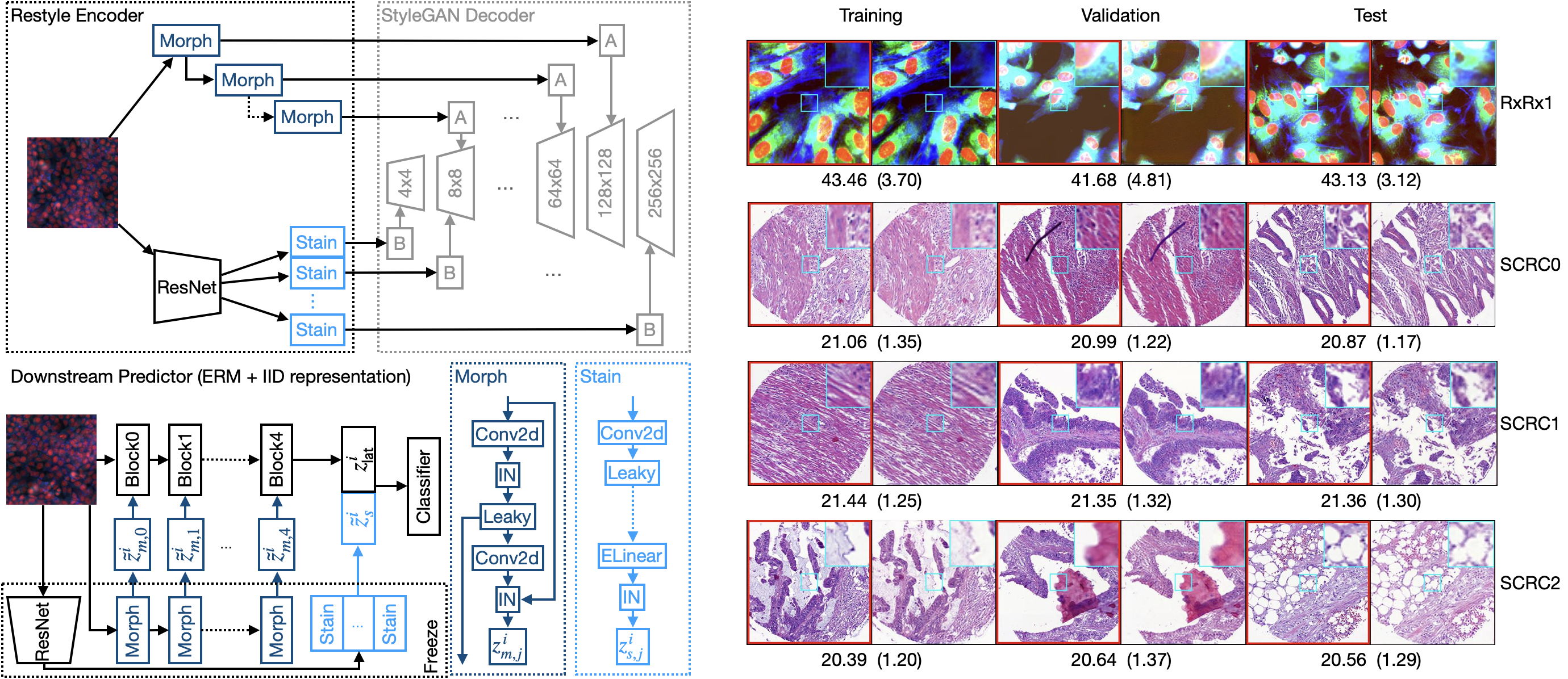
Learning the Approximate IID Representation. Despite being conceptually simple, learning an IID representation that can faithfully reconstruct a given input image is non-trivial. To approximate the IID property and to achieve good reconstruction quality, we propose to utilize the instance normalization (IN) (Ulyanov et al. 2016) in the encoder for proof of concept. Concretely, we apply two kinds of blocks containing IN operations: morphology (morph) and stain to obtain $\mathsf{Z}^{i}\mathrel{\vbox{\hbox{.}\hbox{.}}}=(\underbrace{\mathsf{Z}_{m,0}^{i},\dots,\mathsf{Z}_{m,4}^{i}}_{\mathsf{morph}},\underbrace{\mathsf{Z}_{s,0}^{i},\dots,\mathsf{Z}_{s,13}^{i}}_{\mathsf{stain}})$ in Sec. 3.3 (See Fig. 2). Compared to other normalization strategies (Ioffe and Szegedy 2015; Ba et al. 2016), IN allows to impose the identical mean and standard deviation on the entries of $\mathsf{Z}_{m,0}^{i},\dots,\mathsf{Z}_{m,4}^{i},\mathsf{Z}_{s,0}^{i},\dots,\mathsf{Z}_{s,13}^{i}$ without violating the independence of $\mathsf{Z}^{i}$ (See App. C for more normalization studies). This suggests that the learned representation $\mathsf{Z}^{i}$ is independent and approximately identically distributed.

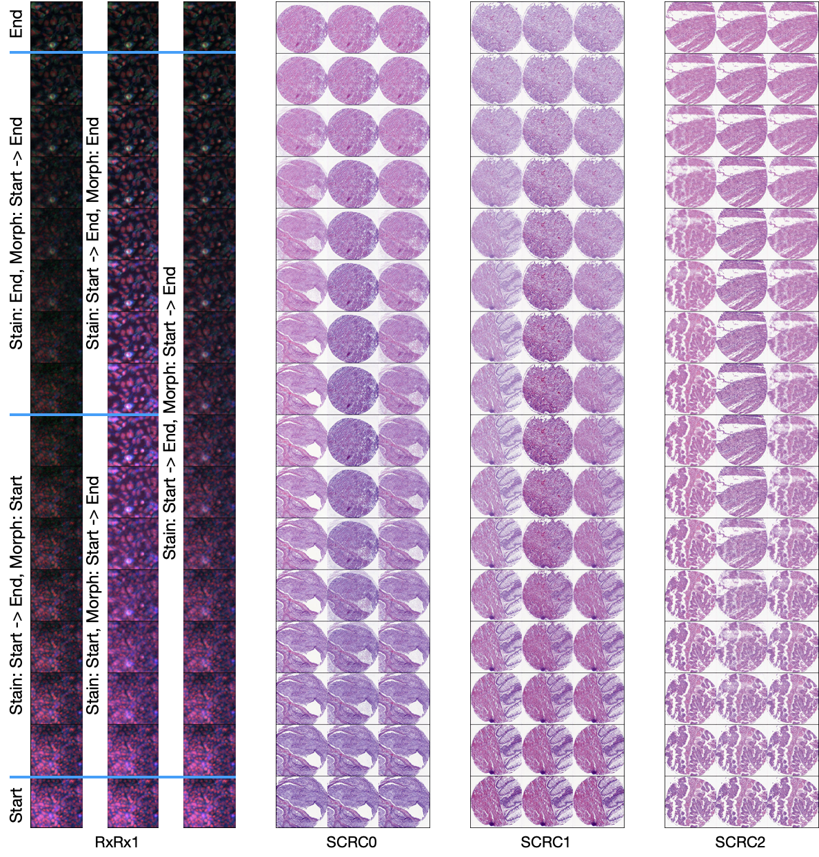
Based on the recent development in image inversion (Alaluf et al. 2021), we instantiate the $\phi,\phi^{\prime}$ in Sec. 3.3 with the Restyle encoder (Alaluf et al. 2021) and StyleGAN decoder (Karras et al. 2020). As shown in Fig. 2 (left), we couple the morph and stain with the noise (A) and style (B) modules of StyleGAN respectively. This is meant for learning a semantic-aware representation for the follow-up interpretation (See Fig. 3). Then, the objective is to reconstruct the input image with $256\times 256$ resolution and defined as $\mathcal{L}=\lambda_{0}\mathcal{L}_{2}+\lambda_{1}\mathcal{L}_{\mathsf{lpips}}+\lambda_{2}\mathcal{L}_{\mathsf{sim}}$ , where $\mathcal{L}_{2}$ is the pixel-wise loss, $\mathcal{L}_{\mathsf{lpips}}$ is the perceptual loss (Tov et al. 2021), $\mathcal{L}_{\mathsf{sim}}$ is the loss measuring the cosine similarity, $\lambda_{0,1,2}$ are the coefficients weighing on the losses. Fig. 2 (right) shows that the approximate IID representation $\mathsf{Z}^{i}$ induced by $\phi$ (Restyle encoder with IN) achieves robust image reconstruction for RxRx1 and SCRC. See App. B, C for more hyper-parameter and result discussions.

The Learned IID Representation in ERM. After freezing the learned Restyle encoder $\phi$ described above, we integrate the $\phi$ induced IID representation $\mathsf{Z}^{i}$ to two standard (ResNet (He et al. 2016), DenseNet (Huang et al. 2017)) and two light-weight (MobileNet (Sandler et al. 2018), MnasNet (Tan et al. 2019)) backbones (See Fig. 2 (left)) that are widely used under the ERM framework. Due to the dimensional compatibility between $\mathsf{Z}_{m,0}^{i},\dots,\mathsf{Z}_{m,4}^{i},\mathsf{Z}_{s,0}^{i},\dots,\mathsf{Z}_{s,13}^{i}$ and layer outputs of the compared backbones, this is implemented via adding the scaled 2-dim output ( $\tilde{\bm{z}}_{m,j}^{i}=\lambda_{m,j}\bm{z}_{m,j}^{i}\;\text{for}\;j=0,\ldots,4$ ) of morph blocks to the block of backbones, and via processing the 1-dim outputs ( $\tilde{\bm{z}}_{s}^{i}=\mathsf{Conv1d}(\mathsf{Cat}(\bm{z}_{s,0}^{i},\ldots,\bm{z}_{s,13}^{i}))$ ) of stain blocks for latent vector concatenation (See also Fig. 2 (left bottom)), where $\lambda_{m,j}$ is a learnable scalar coefficient. Accordingly, the objective is to predict the class of genetic perturbation (RxRx1) and imCMS (SCRC) and defined as $\mathcal{L}=\lambda\mathcal{L}_{\mathsf{crs}}+(1-\lambda)\mathcal{L}_{\mathsf{arc}},$ where $\mathcal{L}_{\mathsf{crs}}$ is the cross-entropy loss, $\mathcal{L}_{\mathsf{arc}}$ is the ArcFace loss (Deng et al. 2019), $\lambda$ is the coefficient balancing the losses. See App. E for more hyper-parameter discussions on SOTA baselines supported in WILDS and proposed method.

[Uncaptioned image] — Table 1: The main results of RxRx1. Top: The average classification accuracies with SD for optimally tuned (Optimal) compared methods (Left) and for ERM and proposed method (Prop) under the same backbones (Right). Bottom: The overall stratified accuracies with SD for ERM and Prop on 4 cell types: HEPG2, HUVEC, RPE, U2OS (Taylor et al. 2019).

Molecular Prediction Result. Surprisingly, the ERM method outperforms the SOTA IRM (ERM + gradient), CORAL (ERM + covariance) and GroupDRO (ERM + worst-case group) in the experiments (See Tab. 1 and 2). More importantly, our proposed method (Prop: ERM + IID representation) achieves top classification accuracies compared to these optimally tuned baselines supported in WILDS for both ID (RxRx1) and OOD test data (SCRC, RxRx1). The consistent improvements under various backbones (Tab. 1 (right) and Tab. 2 (left)) confirm the reusability of learned IID representation. With further stratifying the results by cell types (Tab. 1 (bottom)) and imCMS classes (Tab. 2 (right)) we conclude that the proposed IID representation learning achieves superior results on OOD generalization tasks for RxRx1 and SCRC.

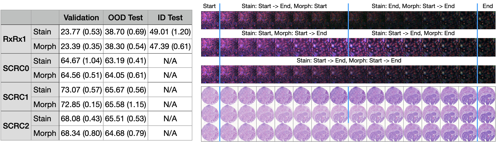
Discussion.When examining stain and morph blocks individually (See Fig. 3), the takeaways are mixed. For RxRx1, the stand-alone stain blocks clearly contribute to the prediction improvement. This may be explained by the preanalytical variation in forms of batch-wise staining shift embedded in validation and test images. For SCRC, neither stain nor morph blocks bring clear quantitative improvements individually. Only by utilizing both of them can we robustify the OOD generalization.

5 Conclusion

In this paper, we propose the IID representation learning and discuss its essential connection to causality. Experimental results on two biomedical datasets show that reusing learned IID representation can improve downstream molecular predictions in terms of OOD generalization. In future work, follow-up investigations from theoretical and biological viewpoints need be conducted to better understand the theoretical guarantee and underlying biological drivers of the IID representation.

\midlacknowledgments

We would like to thank the Colorectal Cancer Research Group and gratefully acknowledge all members of the Translational Research Unit at the Institute of Pathology, University of Bern for excellent collaboration and provision of the CRC image dataset. We gratefully acknowledge the S:CORT consortium, a Medical Research Council stratified medicine consortium led by Prof. Tim Maughan at the University of Oxford, jointly funded by the MRC and CRUK; the current implementation of imCMS is a joint development of the S:CORT consortium at the University of Oxford in particular Prof. Jens Rittscher and Dr. Korsuk Sirinukunwattana at the Department of Engineering Science, Prof. Tim Maughan at the CRUK/MRC Oxford Institute for Radiation Oncology, and Dr. Enric Domingo at the Department of Oncology, University of Oxford with the Computational and Translational Pathology Group at the University of Zurich (Dr. Maxime Lafarge, Prof. Viktor Koelzer). The authors thank Anja Frei for data processing, Sonali Andani and Dr. Marta Nowak for insightful discussion. We gratefully acknowledge funding by the Promedica Foundation F-87701-41-01.

References

Alaluf et al. (2021) Yuval Alaluf, Or Patashnik, and Daniel Cohen-Or. Restyle: A residual-based stylegan encoder via iterative refinement. In Proceedings of the IEEE/CVF International Conference on Computer Vision, pages 6711–6720, 2021.
Angelos (2013) Peter Angelos. Ethical issues of participant recruitment in surgical clinical trials. Annals of surgical oncology, 20(10):3184–3187, 2013.
Arjovsky et al. (2019) Martin Arjovsky, Léon Bottou, Ishaan Gulrajani, and David Lopez-Paz. Invariant risk minimization. arXiv preprint arXiv:1907.02893, 2019.
Ba et al. (2016) Jimmy Lei Ba, Jamie Ryan Kiros, and Geoffrey E Hinton. Layer normalization. arXiv preprint arXiv:1607.06450, 2016.
Balke and Pearl (1995) Alexander Balke and Judea Pearl. Counterfactuals and policy analysis in structural models. In Proceedings of the Eleventh conference on Uncertainty in artificial intelligence, pages 11–18, 1995.
Bareinboim (2014) Elias Bareinboim. Generalizability in causal inference: Theory and algorithms. PhD thesis, UCLA, 2014.
Bareinboim and Pearl (2014) Elias Bareinboim and Judea Pearl. Transportability from multiple environments with limited experiments: Completeness results. In Advances in neural information processing systems, pages 280–288, 2014.
Caldwell et al. (2004) Patrina HY Caldwell, Sharon B Murphy, Phyllis N Butow, and Jonathan C Craig. Clinical trials in children. The Lancet, 364(9436):803–811, 2004.
Chen et al. (2020) Xinlei Chen, Haoqi Fan, Ross Girshick, and Kaiming He. Improved baselines with momentum contrastive learning. arXiv preprint arXiv:2003.04297, 2020.
Chickering (1996) David Maxwell Chickering. Learning bayesian networks is np-complete. In Learning from data, pages 121–130. Springer, 1996.
Cios and Moore (2002) Krzysztof J Cios and G William Moore. Uniqueness of medical data mining. Artificial intelligence in medicine, 26(1-2):1–24, 2002.
de Boer et al. (2019) Stephanie M de Boer, Melanie E Powell, Linda Mileshkin, Dionyssios Katsaros, Paul Bessette, Christine Haie-Meder, Petronella B Ottevanger, Jonathan A Ledermann, Pearly Khaw, Romerai D’Amico, et al. Adjuvant chemoradiotherapy versus radiotherapy alone in women with high-risk endometrial cancer (portec-3): patterns of recurrence and post-hoc survival analysis of a randomised phase 3 trial. The Lancet Oncology, 20(9):1273–1285, 2019.
Deng et al. (2019) Jiankang Deng, Jia Guo, Niannan Xue, and Stefanos Zafeiriou. Arcface: Additive angular margin loss for deep face recognition. In Proceedings of the IEEE/CVF Conference on Computer Vision and Pattern Recognition, pages 4690–4699, 2019.
Farrell et al. (2020) Ruth Farrell, Marsha Michie, and Rachel Pope. Pregnant women in trials of covid-19: a critical time to consider ethical frameworks of inclusion in clinical trials. Ethics & human research, 42(4):17–23, 2020.
Gamella and Heinze-Deml (2020) Juan L Gamella and Christina Heinze-Deml. Active invariant causal prediction: Experiment selection through stability. arXiv preprint arXiv:2006.05690, 2020.
Ganin et al. (2016) Yaroslav Ganin, Evgeniya Ustinova, Hana Ajakan, Pascal Germain, Hugo Larochelle, François Laviolette, Mario Marchand, and Victor Lempitsky. Domain-adversarial training of neural networks. The journal of machine learning research, 17(1):2096–2030, 2016.
Gong et al. (2016) Mingming Gong, Kun Zhang, Tongliang Liu, Dacheng Tao, Clark Glymour, and Bernhard Schölkopf. Domain adaptation with conditional transferable components. In International conference on machine learning, pages 2839–2848. PMLR, 2016.
Goodfellow et al. (2014) Ian Goodfellow, Jean Pouget-Abadie, Mehdi Mirza, Bing Xu, David Warde-Farley, Sherjil Ozair, Aaron Courville, and Yoshua Bengio. Generative adversarial nets. Advances in neural information processing systems, 27, 2014.
He et al. (2016) Kaiming He, Xiangyu Zhang, Shaoqing Ren, and Jian Sun. Deep residual learning for image recognition. In Proceedings of the IEEE conference on computer vision and pattern recognition, pages 770–778, 2016.
Heinze-Deml et al. (2018) Christina Heinze-Deml, Jonas Peters, and Nicolai Meinshausen. Invariant causal prediction for nonlinear models. Journal of Causal Inference, 6(2), 2018.
Hernán and Robins (2020) MA Hernán and JM Robins. Causal inference: What if. Boca Raton: Chapman & Hill/CRC, 2020.
Heusel et al. (2017) Martin Heusel, Hubert Ramsauer, Thomas Unterthiner, Bernhard Nessler, and Sepp Hochreiter. Gans trained by a two time-scale update rule converge to a local nash equilibrium. In Advances in neural information processing systems, pages 6626–6637, 2017.
Huang et al. (2017) Gao Huang, Zhuang Liu, Laurens Van Der Maaten, and Kilian Q Weinberger. Densely connected convolutional networks. In Proceedings of the IEEE conference on computer vision and pattern recognition, pages 4700–4708, 2017.
Ioffe and Szegedy (2015) Sergey Ioffe and Christian Szegedy. Batch normalization: Accelerating deep network training by reducing internal covariate shift. In International conference on machine learning, pages 448–456. PMLR, 2015.
Karamitopoulou et al. (2011) Eva Karamitopoulou, Inti Zlobec, Ioannis Panayiotides, Efstratios S Patsouris, George Peros, George Rallis, Christos Lapas, Petros Karakitsos, Luigi M Terracciano, and Alessandro Lugli. Systematic analysis of proteins from different signaling pathways in the tumor center and the invasive front of colorectal cancer. Human pathology, 42(12):1888–1896, 2011.
Karras et al. (2019) Tero Karras, Samuli Laine, and Timo Aila. A style-based generator architecture for generative adversarial networks. In Proceedings of the IEEE/CVF Conference on Computer Vision and Pattern Recognition, pages 4401–4410, 2019.
Karras et al. (2020) Tero Karras, Samuli Laine, Miika Aittala, Janne Hellsten, Jaakko Lehtinen, and Timo Aila. Analyzing and improving the image quality of stylegan. In Proceedings of the IEEE/CVF Conference on Computer Vision and Pattern Recognition, pages 8110–8119, 2020.
Koh et al. (2021) Pang Wei Koh, Shiori Sagawa, Sang Michael Xie, Marvin Zhang, Akshay Balsubramani, Weihua Hu, Michihiro Yasunaga, Richard Lanas Phillips, Irena Gao, Tony Lee, et al. Wilds: A benchmark of in-the-wild distribution shifts. In International Conference on Machine Learning, pages 5637–5664. PMLR, 2021.
Krizhevsky et al. (2012) Alex Krizhevsky, Ilya Sutskever, and Geoffrey E Hinton. Imagenet classification with deep convolutional neural networks. Advances in neural information processing systems, 25:1097–1105, 2012.
Long et al. (2018) Mingsheng Long, Zhangjie Cao, Jianmin Wang, and Michael I Jordan. Conditional adversarial domain adaptation. In NeurIPS, 2018.
Luo et al. (2020) Yunan Luo, Jian Peng, and Jianzhu Ma. When causal inference meets deep learning. Nature Machine Intelligence, 2(8):426–427, 2020.
Martin et al. (2017) Linda Martin, Melissa Hutchens, Conrad Hawkins, and Alaina Radnov. How much do clinical trials cost. Nat Rev Drug Discov, 16(6):381–382, 2017.
Muandet et al. (2013) Krikamol Muandet, David Balduzzi, and Bernhard Schölkopf. Domain generalization via invariant feature representation. In International Conference on Machine Learning, pages 10–18. PMLR, 2013.
Nguyen et al. (2021) Huu-Giao Nguyen, Oxana Lundström, Annika Blank, Heather Dawson, Alessandro Lugli, Maria Anisimova, and Inti Zlobec. Image-based assessment of extracellular mucin-to-tumor area predicts consensus molecular subtypes (cms) in colorectal cancer. Modern Pathology, pages 1–9, 2021.
Nout et al. (2010) Remi Abubakar Nout, VTHBM Smit, Hein Putter, Ina M Juergenliemk-Schulz, Jan J Jobsen, LCHW Lutgens, Elzbieta M van der Steen-Banasik, Jan Willem M Mens, Annerie Slot, MC Stenfert Kroese, et al. Vaginal brachytherapy versus pelvic external beam radiotherapy for patients with endometrial cancer of high-intermediate risk (portec-2): an open-label, non-inferiority, randomised trial. The Lancet, 375(9717):816–823, 2010.
Pan and Yang (2009) Sinno Jialin Pan and Qiang Yang. A survey on transfer learning. IEEE Transactions on knowledge and data engineering, 22(10):1345–1359, 2009.
Pan et al. (2010) Sinno Jialin Pan, Ivor W Tsang, James T Kwok, and Qiang Yang. Domain adaptation via transfer component analysis. IEEE transactions on neural networks, 22(2):199–210, 2010.
Pearl and Mackenzie (2018) Judea Pearl and Dana Mackenzie. The book of why: the new science of cause and effect. Basic Books, 2018.
Pearl et al. (2000) Judea Pearl et al. Models, reasoning and inference. Cambridge, UK: CambridgeUniversityPress, 19, 2000.
Pearl et al. (2009) Judea Pearl et al. Causal inference in statistics: An overview. Statistics surveys, 3:96–146, 2009.
Peters et al. (2016) Jonas Peters, Peter Bühlmann, and Nicolai Meinshausen. Causal inference by using invariant prediction: identification and confidence intervals. Journal of the Royal Statistical Society. Series B (Statistical Methodology), pages 947–1012, 2016.
Peters et al. (2017) Jonas Peters, Dominik Janzing, and Bernhard Schölkopf. Elements of causal inference. The MIT Press, 2017.
Rojas-Carulla et al. (2018) Mateo Rojas-Carulla, Bernhard Schölkopf, Richard Turner, and Jonas Peters. Invariant models for causal transfer learning. The Journal of Machine Learning Research, 19(1):1309–1342, 2018.
Rosenfeld et al. (2021) Elan Rosenfeld, Pradeep Ravikumar, and Andrej Risteski. The risks of invariant risk minimization. In International Conference on Learning Representations, volume 9, 2021.
Sagawa et al. (2020) Shiori Sagawa, Pang Wei Koh, Tatsunori B Hashimoto, and Percy Liang. Distributionally robust neural networks for group shifts: On the importance of regularization for worst-case generalization. The 7th International Conference on Learning Representations, 2020.
Sandler et al. (2018) Mark Sandler, Andrew Howard, Menglong Zhu, Andrey Zhmoginov, and Liang-Chieh Chen. Mobilenetv2: Inverted residuals and linear bottlenecks. In Proceedings of the IEEE conference on computer vision and pattern recognition, pages 4510–4520, 2018.
Schölkopf et al. (2021) Bernhard Schölkopf, Francesco Locatello, Stefan Bauer, Nan Rosemary Ke, Nal Kalchbrenner, Anirudh Goyal, and Yoshua Bengio. Toward causal representation learning. Proceedings of the IEEE, 109(5):612–634, 2021.
Shapiro and Msaouel (2021) Daniel D Shapiro and Pavlos Msaouel. Causal diagram techniques for urologic oncology research. Clinical genitourinary cancer, 19(3):271–e1, 2021.
Shen et al. (2021) Zheyan Shen, Jiashuo Liu, Yue He, Xingxuan Zhang, Renzhe Xu, Han Yu, and Peng Cui. Towards out-of-distribution generalization: A survey. arXiv preprint arXiv:2108.13624, 2021.
Sirinukunwattana et al. (2020) K Sirinukunwattana, E Domingo, S Richman, K Redmond, A Blake, C Verrill, S Leedham, A Chatzipli, C Hardy, C Whalley, C Wu, A Beggs, U McDermott, P Dunne, A Meade, S Walker, G Murray, L Samuel, M Seymour, I Tomlinson, P Quirke, T Maughan, J Rittscher, and VH Koelzer. Image-based consensus molecular subtype classification (imcms) of colorectal cancer using deep learning. Gut, 2020.
Sun and Saenko (2016) Baochen Sun and Kate Saenko. Deep coral: Correlation alignment for deep domain adaptation. In European conference on computer vision, pages 443–450. Springer, 2016.
Sun et al. (2016) Baochen Sun, Jiashi Feng, and Kate Saenko. Return of frustratingly easy domain adaptation. In Proceedings of the AAAI Conference on Artificial Intelligence, volume 30, 2016.
Tan et al. (2019) Mingxing Tan, Bo Chen, Ruoming Pang, Vijay Vasudevan, Mark Sandler, Andrew Howard, and Quoc V Le. Mnasnet: Platform-aware neural architecture search for mobile. In Proceedings of the IEEE/CVF Conference on Computer Vision and Pattern Recognition, pages 2820–2828, 2019.
Taylor et al. (2019) J Taylor, B Earnshaw, B Mabey, M Victors, and J Yosinski. Rxrx1: An image set for cellular morphological variation across many experimental batches. In The 7th International Conference on Learning Representations, 2019.
Tov et al. (2021) Omer Tov, Yuval Alaluf, Yotam Nitzan, Or Patashnik, and Daniel Cohen-Or. Designing an encoder for stylegan image manipulation. ACM Transactions on Graphics (TOG), 40(4):1–14, 2021.
Ulyanov et al. (2016) Dmitry Ulyanov, Andrea Vedaldi, and Victor Lempitsky. Instance normalization: The missing ingredient for fast stylization. arXiv preprint arXiv:1607.08022, 2016.
Vapnik (1992) Vladimir Vapnik. Principles of risk minimization for learning theory. In Advances in neural information processing systems, pages 831–838, 1992.
Vapnik (1999) Vladimir Vapnik. The nature of statistical learning theory. Springer science & business media, 1999.
Wang and Deng (2018) Mei Wang and Weihong Deng. Deep visual domain adaptation: A survey. Neurocomputing, 312:135–153, 2018.
Wu and He (2018) Yuxin Wu and Kaiming He. Group normalization. In Proceedings of the European conference on computer vision (ECCV), pages 3–19, 2018.
Yun et al. (2019) Sangdoo Yun, Dongyoon Han, Seong Joon Oh, Sanghyuk Chun, Junsuk Choe, and Youngjoon Yoo. Cutmix: Regularization strategy to train strong classifiers with localizable features. In Proceedings of the IEEE/CVF International Conference on Computer Vision, pages 6023–6032, 2019.
Zhang et al. (2018) Richard Zhang, Phillip Isola, Alexei A Efros, Eli Shechtman, and Oliver Wang. The unreasonable effectiveness of deep features as a perceptual metric. In Proceedings of the IEEE conference on computer vision and pattern recognition, pages 586–595, 2018.
Zhuang et al. (2020) Fuzhen Zhuang, Zhiyuan Qi, Keyu Duan, Dongbo Xi, Yongchun Zhu, Hengshu Zhu, Hui Xiong, and Qing He. A comprehensive survey on transfer learning. Proceedings of the IEEE, 109(1):43–76, 2020.

Appendix A Toy Experiments for Causal Variable Identification

Complementary to Sec. 4, we conduct toy experiments on the causal variable identification task (Sec. 3.1) for validating the proposed IID representation learning. This is done by following the experimental design of AICP Gamella and Heinze-Deml 2020 (Please see also https://github.com/juangamella/aicp). Specifically, we start the data simulation by creating a directed acyclic graph (DAG) endowed with vertices, edges and Gaussian noises, where the vertices of the DAG correspond to the variables $\mathsf{x}_{0},\mathsf{x}_{1},\ldots,\mathsf{x}_{l}$ in Sec. 3.1. These specifications form a linear Gaussian SCM.

W.l.o.g. consider $\mathsf{x}_{0}$ be the outcome variable and $\mathsf{X_{PA_{0}}}$ be the set of $\mathsf{x}_{0}$ ’s parent variables, under the assumption of without intervening on the outcome $\mathsf{x}_{0}$ , we implement do-interventions $e_{j=1,\ldots,l}$ independently via breaking the edges pointing to $\mathsf{x}_{j}$ and letting $\mathsf{x}_{j}\mathrel{\vbox{\hbox{.}\hbox{.}}}=c$ , which simulates the RCT setting described in Sec. 3.1. As specified in https://github.com/juangamella/aicp, we then collect $l$ batches of data samples that are randomly drawn from the SCM intervened with $e_{j=1,\ldots,l}$ resp. In the same manner as AICP Gamella and Heinze-Deml 2020, given such a dataset, our goal is to identify the set of parent variables of the outcome $\mathsf{x}_{0}$ .

Instead of a sophisticated auto-encoder proposed in Sec. 4, here we utilize a simple neural network $\phi^{\prime}\circ\phi$ , where $\phi^{\prime}$ is a standard MLP layer, $\phi(\bm{x})=\bm{w}\odot\bm{x}$ is the element-wise multiplication of the input $\bm{x}$ and binary penalty weights $\bm{w}$ (initialized with 1). We propose to learn the projection map $\phi$ inducing identical interventional distribution among $(\mathsf{X_{PA_{0}}^{e_{j}}},\mathsf{x_{0}})$ for $j=1,\ldots,l$ , where $\phi$ should project $\{\mathsf{x}_{1},\ldots,\mathsf{x}_{l}\}$ to $\mathsf{X_{PA_{0}}}$ . Noting that $\phi$ also induces independence among $(\mathsf{X_{PA_{0}}^{e_{j}}},\mathsf{x_{0}})$ for $j=1,\ldots,l$ due to the independently intervened SCMs. Concretely, we train $\phi^{\prime}\circ\phi$ for $l$ epochs with $\|.\|_{2}$ norm and iteratively penalize if $\mathsf{x_{j}}\in\mathsf{X_{PA_{0}}}$ holds true ( $w_{j}$ of $\phi$ remains to be 1) for $j=1,\ldots,l$ per epoch. Such penalty is conditioned on $\max_{j=1,\ldots,l}\mathsf{FID}\,(\mu_{j},\mu_{j^{c}}),$ where $\mathsf{FID}$ is the Fréchet inception distance Heusel et al. 2017, $\mu_{j},\mu_{j^{c}}$ are the interventional distributions of $\|\phi^{\prime}\circ\phi(x_{1},\ldots,x_{l})-x_{0}\|_{2}$ w.r.t. the data sampled from $\{e_{j}\}$ and $\{e_{1},\ldots,e_{l}\}\setminus\{e_{j}\}$ intervened SCM(s) resp.

	Jaccard Similarity (FWER)
ICP	0.318 (1.00)	0.401 (0.84)	1.00 (0.00)
NICP	0.317 (1.00)	0.406 (0.82)	1.00 (0.00)
AICP	0.438 (0.05)	0.485 (0.11)	1.00 (0.00)
Proposed	0.909 (0.16)	0.926 (0.12)	1.00 (0.00)

Then we compare the proposed method with ICP Peters et al. 2016, NICP Heinze-Deml et al. 2018 and AICP, all of which are developed upon the idea of identifying $\mathsf{X_{PA_{0}}}$ via the intersection of sets of plausible causal variables. To better examine the robustness of compared methods, not only do we randomly choose $50$ DAGs to re-run the experiments but additionally introduce 1 and 2 hidden confounder(s) for each DAG resp. As shown in Tab. 3, our proposed IID representation learning outperforms the ICPs especially with the inclusion of hidden confounder(s), in terms of better Jaccard Similarity (JS) and Family-wise error rate (FWER) Gamella and Heinze-Deml 2020 averaged on $50$ DAGs,

\mathsf{JS}(\mathsf{Z},\mathsf{X_{PA_{0}}})=\frac{|\mathsf{Z}\cap\mathsf{X_{PA_{0}}}|}{|\mathsf{Z}\cup\mathsf{X_{PA_{0}}}|},\;\mathsf{FWER}=\mathbb{P}(\mathsf{Z}\nsubseteq\mathsf{X_{PA_{0}}}),\text{where }\mathsf{Z}=\phi(\mathsf{x}_{1},\ldots,\mathsf{x}_{l})=(w_{1}x_{1},\ldots,w_{l}x_{l}).

(3)

Appendix B Unsupervised Training of StyleGAN Decoder

Since there are not pre-trained StyleGAN (Karras et al. 2020) decoders available for the IID representation learning on RxRx1 and SCRC, we start the experiments with training StyleGAN in an unsupervised manner. Concretely, we take the widely-used PyTorch implementation https://github.com/rosinality/stylegan2-pytorch for training StyleGAN. Following the suggestions from WILDS, we only utilize the training data of RxRx1 and SCRC0,1,2 to learn four different StyleGAN models that can synthesize visually plausible microscopy images, while the validation and test data are held back during training. Due to the nature of moderate amount of training data, we follow the default configurations of StyleGAN training suggested in the repository except that we customize the training iterations to be 100k for all experiments, batch size to be 32 for RxRx1 and 16 for SCRC. Then we take advantage of the Distributed Data-Parallel (DDP) mechanism provided in PyTorch and train the StyGAN models on 4 A-100 GPUs and 2 A-100 GPUs for RxRx1 and SCRC respectively. We report the average Fréchet inception distance (FID) (Heusel et al. 2017) scores with SD obtained with four different random seeds for all the experiments in Tab. 4 and demonstrate the non-cherry-picked synthesized images in Fig. 4, 5, 6, 7. Noting that the large FID score for RxRx1 is resulted from comparing the total statistical difference on the ensemble of fluorescent medical images with more than $1000$ classes of genetic perturbation, which differs from the common FID score computation in terms of a single class natural image generation (Karras et al. 2019; Karras et al. 2020).

Appendix C Learning the Approximate IID Representation

To achieve faithful microscopy image reconstruction, we utilize the pre-trained StyleGAN decoder discussed in App. B and Restyle encoder (Alaluf et al. 2021) for learning the approximate IID representation. For the perceptual $\mathcal{L}_{\mathsf{lpips}}$ (Zhang et al. 2018; Tov et al. 2021) and cosine similarity $\mathcal{L}_{\mathsf{sim}}$ (Chen et al. 2020) loss of the reconstruction objective, we follow the default configuration introduced in Restyle encoder (Alaluf et al. 2021), i.e., the $\mathcal{L}_{\mathsf{lpips}}$ and $\mathcal{L}_{\mathsf{sim}}$ are computed based on features extracted from the linear layer of the pre-trained AlexNet (Krizhevsky et al. 2012) and the MoCoV2 (Chen et al. 2020) pretrained ResNet50 (He et al. 2016) respectively, see also https://github.com/yuval-alaluf/restyle-encoder for more implementation details. Besides, by tuning on the validation data, it suffices to execute one step for iterative refinement and train all the experiments with 90k iterations. Lastly, the hyper-parameters $\lambda_{0,1,2}$ in the reconstruction objective are determined to be $1.5,0.5,0.5$ and $5,0.2,0.2$ for SCRC0,1,2 and RxRx1 respectively.

With computing the batch-wise statistics, the batch normalization (Ioffe and Szegedy 2015) (BN) introduces unnecessary batch dependence between training data. Because of the element-wise affine operation applied on each image by default, the requirement that learning a function inducing identical distributions cannot be guaranteed by layer normalization (Ba et al. 2016) (LN). In combination of these observations and independent, approximately identically distributed $\mathsf{Z}^{i}$ (Sec. 3.3) obtained via instance normalization (Ulyanov et al. 2016) (IN), we impose IN on the Restyle encoder (including the ResNet backbone). Under the same Restyle architecture, we run experiments and compare the reconstruction performance achieved between IN, BN (utilized in the default Restyle encoder), LN as well as group normalization (Wu and He 2018) (GN). As a result, we experimentally justified the superiority of IN in terms of robust PSNR scores (See Tab. 5) and better visual qualities (See Fig. 8, 9, 10, 11).

Appendix D More Interpolation Visualization

Appendix E The learned IID Representation in ERM

To enable reproducibility and for comparison to the SOTA methods, we utilize the WILDS repository https://github.com/p-lambda/wilds.git to run the experiments. Precisely, we call the data loader functions of RxRx1 implemented in WILDS and write the corresponding data loader functions for SCRC following the WILDS coding style. Except that we introduce the CutMix (Yun et al. 2019) as a complement to the standard augmentation methods supported in WILDS, we do not use additional techniques such as fusing the outputs from several rotated inputs or from multiple models to boost the performance for compared methods. During the training, we do not feed the validation and test data to the model, the validation data is only used for hyper-parameter tuning. Accordingly, all compared methods are well tuned on the hyper-parameters with the careful selection of augmentations, backbones, etc.

For ERM, we determine the optimal $\lambda$ to be $0.8$ and $\lambda_{\mathsf{CutMix}}$ to be $1$ for RxRx1 and SCRC, ResNet50/DenseNet121 for RxRx1 and MobileNetV2 for SCRC. For IRM and CORAL, we determine the optimal $\lambda$ to be $1$ , the backbone to be MobileNetV2 and $\lambda_{\mathsf{CutMix}}=0$ for both RxRx1 and SCRC. In terms of GroupDRO, the configurations are the same to IRM and CORAL except that with utilizing DenseNet121 it achieves competitive results to MobileNetV2 in SCRC experiments. As to the proposed method (Prop), the optimal results are obtained by $\lambda=0.8,\lambda_{\mathsf{CutMix}}=1$ for both RxRx1 and SCRC, as well as ResNet50 for RxRx1 and MobileNetV2 for SCRC. Complementary to the Tab. 1 and 2 in the main manuscript, we present detailed results for all compared methods with respect to the same backbones in Tab. 6 and 7.

	Jaccard Similarity (FWER)
	2 Confounders	1 Confounder	0 Confounder
ICP	0.318 (1.00)	0.401 (0.84)	1.00 (0.00)
NICP	0.317 (1.00)	0.406 (0.82)	1.00 (0.00)
AICP	0.438 (0.05)	0.485 (0.11)	1.00 (0.00)
Proposed	0.909 (0.16)	0.926 (0.12)	1.00 (0.00)

Towards IID representation learning and its application on biomedical data

Abstract

keywords

1 Introduction

2 Proposed Definition

Definition 1.

Remark 1.

Remark 2.

3 From Causality to IID

3.1 Causal Variable Identification →\to IID symmetry

Question.

Discussion.

3.2 Causal Effect Transportation →\to IID Generalization

Question.

Discussion.

3.3 Causal Feature Representation →\to IID Representation

Question.

Discussion.

4 OOD Experiment

5 Conclusion

References

Appendix A Toy Experiments for Causal Variable Identification

Appendix B Unsupervised Training of StyleGAN Decoder

Appendix C Learning the Approximate IID Representation

Appendix D More Interpolation Visualization

Appendix E The learned IID Representation in ERM

3.1 Causal Variable Identification $\to$ IID symmetry

3.2 Causal Effect Transportation $\to$ IID Generalization

3.3 Causal Feature Representation $\to$ IID Representation