跳到论文正文
W Papers独立论文阅读器 arXiv:2203.00246 论文正文 计算阅读时间 · 0%
引用这篇论文根据当前论文元数据生成,正式投稿前建议核对。


License: CC BY 4.0
arXiv:2203.00246v6 [cs.LG] 24 Mar 2023

Hong Jun Jeon and Yifan Zhu and Benjamin Van Roy

An Information-Theoretic Framework for
Supervised Learning

Hong Jun Jeon hjjeon@stanford.edu Affiliation: Department of Computer Science Affiliation: Stanford University Affiliation: Stanford, CA 94305, USA    Yifan Zhu zhuyifan@stanford.edu Affiliation: Department of Electrical Engineering Affiliation: Stanford University Affiliation: Stanford, CA 94305, USA    Benjamin Van Roy bvr@stanford.edu Affiliation: Stanford University Affiliation: Stanford, CA 94305, USA
Abstract

Each year, deep learning demonstrates new and improved empirical results with deeper and wider neural networks. Meanwhile, with existing theoretical frameworks, it is difficult to analyze networks deeper than two layers without resorting to counting parameters or encountering sample complexity bounds that are exponential in depth. Perhaps it may be fruitful to try to analyze modern machine learning under a different lens. In this paper, we propose a novel information-theoretic framework with its own notions of regret and sample complexity for analyzing the data requirements of machine learning. With our framework, we first work through some classical examples such as scalar estimation and linear regression to build intuition and introduce general techniques. Then, we use the framework to study the sample complexity of learning from data generated by deep neural networks with ReLU activation units. For a particular prior distribution on weights, we establish sample complexity bounds that are simultaneously width independent and linear in depth. This prior distribution gives rise to high-dimensional latent representations that, with high probability, admit reasonably accurate low-dimensional approximations. We conclude by corroborating our theoretical results with experimental analysis of random single-hidden-layer neural networks.

††heading: 1 2021 ††shortheadings: An Information-Theoretic Framework for Supervised Learning / Jeon and Van Roy††firstpage: 1
keywords
information theory, rate-distortion theory, neural networks

1 Introduction

The refrain “success is guaranteed” espoused by some deep learning researchers suggests that, given a large data set, a sufficiently large neural network trained via stochastic gradient descent will deliver a useful model. Perhaps this statement is not intended to be taken literally, as it is easy to generate data in a manner for which no algorithm can accomplish this by learning from any reasonable number of samples. Yet, neural networks have successfully addressed many complex data sets. This begs the question: “for what data generating processes can neural networks succeed?”

Perhaps this refrain stems from the empirical phenomena of this era. In modern machine learning, the apparent capabilities of empirical methods have rapidly outpaced what is soundly understood theoretically. Modern neural network architectures have scaled immensely in both parameter count and depth. GPT3 for example has  175 billion parameters and 96 decoder blocks, each with many layers within. Yet, contrary to traditional statistical analyses, these deep neural networks with gargantuan parameter counts are able to generalize well and produce useful models. This gap between what has been shown theoretically versus empirically makes it quite enticing to develop a coherent framework that could explain this phenomenon.

In parametric statistics, the number of parameters typically drives sample complexity. In the realm of classical statistics, problems such as linear regression, this analysis based on parameter count can produce sharp results that mirror what is observed in practice. Naturally, researchers have made efforts to extend these techniques to try and understand deep learning.

However, these existing results break down when trying to explain learning under models that are simultaneously very deep (many layers) and wide (many hidden units per layer). Classical results such as those of Haussler 1992 and Bartlett et al. 1998 can potentially handle the deep but narrow case. These results bound the sample complexity of a learning a neural network function in terms of the number of parameters and the depth. More recently, Harvey et al. 2017 established a general result that suggests that for neural networks with piecewise-linear activation units, the sample complexity grows linearly in the product of parameter count and depth. However, when we consider neural networks with arbitrary width, these bounds become vacuous. This is unnerving as in practice, wider neural networks have been observed to generalize better (Neyshabur et al. 2014).

As an alternative to parameter count methods, researchers have produced sample complexity bounds that depend on the product of norms of realized weight matrices. In these networks, while the layers may be arbitrarily wide, the complexity is instead constrained by bounded weight matrix norms. Bartlett et al. 2017 and Neyshabur et al. 2018a, for example, establish sample complexity bounds that scale with the product of spectral norms. Neyshabur et al. 2015 and Golowich et al. 2018 establish similar bounds that instead scale in the product of Frobenius norms. While this line of work provides sample complexity bounds that are width-independent, they pay for it via an exponential dependence on depth, which is also inconsistent with empirical results.

A large line of work has tried to ameliorate this exponential depth dependence via so-called data-dependent quantities (Dziugaite and Roy 2017; Arora et al. 2018; Nagarajan and Kolter 2018; Wei and Ma 2019). Among these, the most relevant to our work is Wei and Ma 2019, which bounds sample complexity as a function of depth and statistics of trained neural network weights. While difficult to interpret due to dependence on complicated data-dependent statistics, their bound suggests a nonic dependence on depth. Arora et al. 2018 also utilize concepts of compression in their analysis, which we generalize and expand upon. While they establish a sample complexity bound that suggests quadratic dependence on depth, further dependence may be hidden in data-dependent terms. These data-dependent bounds are touted for their flexibility as one can derive expected error bounds by simply integrating out randomness of the data. However, such a procedure does not allow one to derive the bounds that we establish in this paper.

The results in computational theory would suggest a similarly bleak picture. They suggests that, even for single-hidden-layer teacher networks, the computation required to achieve this sample complexity is intractable. For example, Goel et al. 2020; Diakonikolas et al. 2020 establish that, for batched stochastic gradient descent with respect to squared or logistic loss to achieve small generalization error for all single-hidden-layer teacher networks, the number of samples or number of gradient steps must be superpolynomial in input dimension or network width. Furthermore, current theoretical guarantees for all computationally tractable algorithms proposed for fitting single-hidden-layer teacher networks with parameters drawn from natural distributions only bound sample complexity by high-order polynomial (Janzamin et al. 2015; Ge et al. 2017) or exponential (Zhong et al. 2017; Fu et al. 2020) functions of input dimension or width.

We suspect that the looseness of all aforementioned results in comparison to empirical findings is due to the worst-case analysis framework. In this paper, we study an average-case notions of regret and sample complexity that are motivated by information theory. Our information-theoretic framework generalizes that developed by Haussler et al. 1994, which provided a basis for understanding the relationship between prediction error and information. In a similar vein, Russo and Zou 2019 introduced tools that establish general relationships between mutual information and error. Using these results, Xu and Raginsky 2017 established upper bounds on the generalization error of learning algorithms with countably infinite hypothesis spaces. We extend these results in several directions to enable analysis of data generating processes related to deep learning. For example, the results of Haussler et al. 1994 do not address noisy observations, and all three aforementioned papers do not accommodate continuous parameter spaces, let alone nonparametric data generating processes. A distinction of our work is that it builds on rate-distortion theory to address these limitations. While Nokleby et al. 2016 also use rate-distortion theory to study Bayes risk, these results are again limited to parametric classification and only offer lower bounds. The rate-distortion function that we study is equivalent to one defined by the information bottleneck (Tishby et al. 2000). However, instead of using it as a basis for optimization methods as do Shwartz-Ziv and Tishby 2017, we develop tools to study sample complexity and arrive at concrete and novel results.

In this paper, we consider contexts in which an agent learns from an iid sequence of data pairs. We consider a suite of data generating processes ranging from classical examples to those for which deep neural networks may be suited. For each data generating process, we quantify the number of samples required to arrive at a useful model. These analyses rely on general and elegant information-theoretic results that we introduce. We establish tight upper and lower bounds for the average regret and sample complexity that depend on the rate-distortion function. With these information-theoretic tools, we analyze three deep neural network data generating processes and quantify the number of samples required to arrive at a useful model. For a ReLU deep neural network with independent weights, we establish novel sample complexity bounds that are roughly linear in the parameter count (as opposed to linear in the product of parameter count and depth as established in (Harvey et al. 2017)). For a ReLU deep neural network with weights drawn from an appropriately scaled Dirichlet distribution, we establish sample complexity bounds that are, within logarithmic factors, linear in depth and independent of width as opposed to exponential (Bartlett et al. 2017) or high-order polynomial (Wei and Ma 2019) in depth. Despite the fact that these bounds are prescribed for an optimal learner, we provide extensive computational evidence that, in practice, the performance of agents that apply stochastic gradient descent (SGD) and automated width selection closely approximates our bounds, even though they pertain to optimal learners.

We view our approach to bounding sample complexity of multilayer data generating processes, our foundational information-theoretic tools, and our extensive experimental verification to be the primary contributions of this paper. Beyond this paper, we expect future results to build on this framework. In particular, its generality and conceptual simplicity positions it to address problems beyond supervised learning, such as reinforcement learning (Sutton and Barto 2018) and learning with side information (Jonschkowski et al. 2015). Indeed, information theory has already influenced thought on these topics (Lu et al. 2021), and our results should provide tools to develop further understanding.

2 Prediction and Error

Consider an environment which, when presented with an input, responds with an output. In the standard framing of supervised learning, an agent learns from input-output data pairs to predict the output corresponding to any future input. Accuracy of the agent’s prediction depends on information the agent has acquired about the environment. In this section, we introduce mathematical formalisms for reasoning about environments and predictions. We formalize a notion of error that is equivalent to the incremental information that a new data pair provides about the environment. With this notion of error, we establish the notions of regret and sample complexity that we will study in this work. While to many these ideas may seem unconventional, we provide connections between our formalism and existing hallmarks of machine learning.

2.1 Environment

We denote input and output spaces by 𝒳\mathcal{X} and 𝒴\mathcal{Y}. While our concepts and results extend to more general spaces, for the purpose of this paper, we restrict attention to cases where 𝒳\mathcal{X} is a finite-dimensional real-valued vector space and 𝒴\mathcal{Y} is also a finite-dimensional real-valued vector space (regression) or finite (classification). As illustrated in Figure 1, an environment ℰ\mathcal{E} prescribes to each input XX and a conditional probability measure ℰ(⋅|X)\mathcal{E}(\cdot|X) of the output YY.

Refer to caption
Figure 1: Presented with an input, an environment responds with an output.

In order to model the agent’s uncertainty about the environment, we treat ℰ\mathcal{E} as a random variable. Before gathering any data, the agent’s beliefs about the environment are represented by the prior distribution ℙ(ℰ∈⋅)\mathbb{P}(\mathcal{E}\in\cdot). The agent’s beliefs evolve as it conditions this distribution on observations.

2.2 Data Generating Process

We consider a stochastic process that generates a sequence ((Xt,Yt+1):t=0,…,T−1)((X_{t},Y_{t+1}):t=0,\ldots,T-1) of data pairs. We refer to each XtX_{t} as an input and each Yt+1Y_{t+1} as an output. We define these and all other random variables we will consider with respect to a probability space (Ω,𝔽,ℙ)(\Omega,\mathbb{F},\mathbb{P}).

Elements of the sequence (Xt:t=0,…,T−1)(X_{t}:t=0,\ldots,T-1) are iid. Denote the history of data generated through time tt by Ht=(X0,Y1,…,Xt−1,Yt,Xt)H_{t}=(X_{0},Y_{1},\ldots,X_{t-1},Y_{t},X_{t}). Each output is distributed according to ℙ(Yt+1∈⋅|ℰ,Ht)=ℰ(⋅|Xt)\mathbb{P}(Y_{t+1}\in\cdot|\mathcal{E},H_{t})=\mathcal{E}(\cdot|X_{t}). Here, ℰ\mathcal{E} (the environment) is a random function that specifies a conditional output distribution ℰ(⋅|x)\mathcal{E}(\cdot|x) for each input xx. As aforementioned, initial uncertainty about ℰ\mathcal{E} is expressed by the prior distribution ℙ(ℰ∈⋅)\mathbb{P}(\mathcal{E}\in\cdot). Note that, conditioned on ℰ\mathcal{E}, the sequence ((Xt,Yt+1):t=0,…,T−1)((X_{t},Y_{t+1}):t=0,\ldots,T-1) is iid.

2.3 Prediction

We consider an agent that predicts the next output Yt+1Y_{t+1} given the history HtH_{t}. Rather than a point estimate, the agent provides as its prediction a probability distribution PtP_{t} over possible outputs. We characterize the agent in terms of a function π\pi for which Pt=π⁡(Ht)P_{t}=\pi(H_{t}).

It will be useful to introduce some notation for referring to particular predictions. We will generally use PtP_{t} as a dummy variable – that is a generic prediction whose definition depends on context. We denote the prediction conditioned on the environment, which could only be produced by a prescient agent, by

Pt∗=ℙ(Yt+1∈⋅|ℰ,Xt)=ℰ(⋅|Xt).P^{*}_{t}=\mathbb{P}(Y_{t+1}\in\cdot|\mathcal{E},X_{t})=\mathcal{E}(\cdot|X_{t}).

We will refer to this as the target distribution as it represents what an agent aims to learn. Finally, we denote by P^t\hat{P}_{t} the posterior-predictive

P^t=ℙ(Yt+1∈⋅|Ht),\hat{P}_{t}=\mathbb{P}(Y_{t+1}\in\cdot|H_{t}),

which will turn out to be optimal for the objective we will define next.

2.4 Error

We assess the error of a prediction PtP_{t} in terms of the KL-divergence relative to Pt∗P^{*}_{t}:

𝐝KL(Pt∗∥Pt)=∫Pt∗(dy)lnd​Pt∗d​Pt(y).\mathbf{d}_{\mathrm{KL}}(P^{*}_{t}\|P_{t})=\int P^{*}_{t}(dy)\ln\frac{dP^{*}_{t}}{dP_{t}}(y).

This quantifies mismatch between the prediction PtP_{t} and target distribution Pt∗P^{*}_{t}. As the following examples illustrate, this generalizes notions of error, like mean-squared error and cross-entropy loss, that are commonly used in the machine learning literature.

2.5 Connections to Cross-Entropy Loss

We establish that in the classification setting, our notion of error is equivalent to cross-entropy loss up to translations.

Example 0.

(cross-entropy loss) Suppose the set 𝒴\mathcal{Y} of possible outputs is finite. Then,

𝐝KL(P∗∥P)=∑y∈𝒴P∗(y)lnP∗​(y)P⁡(y)=∑y∈𝒴P∗(y)lnP∗(y)−∑y∈𝒴P∗(y)lnP(y).\mathbf{d}_{\mathrm{KL}}(P^{*}\|P)=\sum_{y\in\mathcal{Y}}P^{*}(y)\ln\frac{P^{*}(y)}{P(y)}=\sum_{y\in\mathcal{Y}}P^{*}(y)\ln P^{*}(y)-\sum_{y\in\mathcal{Y}}P^{*}(y)\ln P(y).

The first term of this difference does not depend on PP, so minimizing KL-divergence is equivalent to minimizing the final term,

−∑y∈𝒴P∗(y)lnP(y)=−𝔼[ln(P(Yt+1))|ℰ,P,X],-\sum_{y\in\mathcal{Y}}P^{*}(y)\ln P(y)=-\mathbb{E}[\ln(P(Y_{t+1}))|\mathcal{E},P,X],

which is exactly the expected cross-entropy loss of PP, as is commonly used to assess classifiers.

2.6 Connections to Mean-Squared Error

In the regression setting we first establish a direct link between KL-divergence and mean-squared error for the case in which Pt∗P^{*}_{t} and PtP_{t} are Gaussian.

Example 0.

(gaussian mean-squared error) Fix μ∈ℜ\mu\in\Re and σ2∈ℜ+⁣+\sigma^{2}\in\Re_{++}. Let ℙ(Yt+1∈⋅|ℰ,Xt)∼𝒩(μ,σ2)\mathbb{P}(Y_{t+1}\in\cdot|\mathcal{E},X_{t})\sim\mathcal{N}(\mu,\sigma^{2}). Consider a point prediction μ^t\hat{\mu}_{t} that is determined by HtH_{t} and a distributional prediction Pt∼𝒩⁡(μ^t,σ2)P_{t}\sim\mathcal{N}(\hat{\mu}_{t},\sigma^{2}). Then,

𝐝KL(Pt∗∥Pt)=𝔼[(μ−μ^t)2|ℰ,Ht]2​σ2=𝔼[(Yt+1−μ^t)2|ℰ,Ht]−𝔼[(Yt+1−μt)2|ℰ,Ht]2​σ2.\mathbf{d}_{\mathrm{KL}}(P^{*}_{t}\|P_{t})=\frac{\mathbb{E}[(\mu-\hat{\mu}_{t})^{2}|\mathcal{E},H_{t}]}{2\sigma^{2}}=\frac{\mathbb{E}[(Y_{t+1}-\hat{\mu}_{t})^{2}|\mathcal{E},H_{t}]-\mathbb{E}[(Y_{t+1}-\mu_{t})^{2}|\mathcal{E},H_{t}]}{2\sigma^{2}}.

Hence, KL-divergence grows monotonically with respect to the squared error 𝔼[(Yt+1−μ^t)2|ℰ,Ht]\mathbb{E}[(Y_{t+1}-\hat{\mu}_{t})^{2}|\mathcal{E},H_{t}]. However, while the minimal squared error 𝔼[(Yt+1−μ)2|ℰ,Ht]=σ2\mathbb{E}[(Y_{t+1}-\mu)^{2}|\mathcal{E},H_{t}]=\sigma^{2} that is attainable with full knowledge of the environment remains positive, the minimal KL-divergence, which is delivered by Pt∼𝒩⁡(μ,σ2)P_{t}\sim\mathcal{N}(\mu,\sigma^{2}), is zero.

Now consider a distributional prediction Pt∼𝒩⁡(μ^t,σ^t2)P_{t}\sim\mathcal{N}(\hat{\mu}_{t},\hat{\sigma}_{t}^{2}), based on a variance estimate σ^t2≠σ2\hat{\sigma}_{t}^{2}\neq\sigma^{2}. Then,

𝐝KL(Pt∗∥Pt)=\displaystyle\mathbf{d}_{\mathrm{KL}}(P^{*}_{t}\|P_{t})= 𝔼[(μ−μ^t)2|ℰ,Ht]2​σ^t2+12​(σ2σ^t2−1−ln⁡σ2σ^t2).\displaystyle\frac{\mathbb{E}[(\mu-\hat{\mu}_{t})^{2}|\mathcal{E},H_{t}]}{2\hat{\sigma}_{t}^{2}}+\frac{1}{2}\left(\frac{\sigma^{2}}{\hat{\sigma}_{t}^{2}}-1-\ln\frac{\sigma^{2}}{\hat{\sigma}^{2}_{t}}\right).

Consider optimizing the choice of σ^t2\hat{\sigma}^{2}_{t} given HtH_{t}:

minσ^t2𝔼[𝐝KL(Pt∗∥Pt)|Ht].\min_{\hat{\sigma}^{2}_{t}}\mathbb{E}[\mathbf{d}_{\mathrm{KL}}(P^{*}_{t}\|P_{t})|H_{t}].

The minimum is attained by

σ^t2=σ2⏟aleatoric+𝔼⁡[(μ−𝔼⁡[μ|Ht])2|Ht]⏟epistemic+𝔼⁡[(𝔼⁡[μ|Ht]−μ^t)2|Ht]⏟b​i​a​s,\hat{\sigma}^{2}_{t}=\underbrace{\sigma^{2}}_{\rm aleatoric}+\underbrace{\mathbb{E}[(\mu-\mathbb{E}[\mu|H_{t}])^{2}|H_{t}]}_{\rm epistemic}+\underbrace{\mathbb{E}[(\mathbb{E}[\mu|H_{t}]-\hat{\mu}_{t})^{2}|H_{t}]}_{bias},

which differs from σ2\sigma^{2}. While σ2\sigma^{2} characterizes aleatoric uncertainty, the incremental variance σ^t2−σ2\hat{\sigma}^{2}_{t}-\sigma^{2} accounts for epistemic uncertainty and bias.

Now, for Pt∗P_{t}^{*} and PtP_{t} that are not Gaussian, we have the following upper bound:

Lemma 3.

For all t∈ℤ+t\in\mathbb{Z}_{+}, if μ^t=∫y∈𝒴y​d​Pt​(y)\hat{\mu}_{t}=\int_{y\in\mathcal{Y}}y\ dP_{t}(y), then

𝔼[𝐝KL(Pt∗∥Pt)]≤12ln(1+𝔼⁡[(Yt+1−μ^t)2]σ2).\mathbb{E}\left[\mathbf{d}_{\mathrm{KL}}(P_{t}^{*}\|P_{t})\right]\leq\frac{1}{2}\ln\left(1+\frac{\mathbb{E}\left[\left(Y_{t+1}-\hat{\mu}_{t}\right)^{2}\right]}{\sigma^{2}}\right).

Therefore, decreasing the mean squared error will always decrease the expected KL-divergence. A corresponding lower bound holds for data generating processes for which Yt+1Y_{t+1} satisfies a certain subgaussian condition:

Lemma 4.

For all t∈ℤ+t\in\mathbb{Z}_{+}, let μ^t=∫y∈𝒴y​d​Pt​(y)\hat{\mu}_{t}=\int_{y\in\mathcal{Y}}y\ dP_{t}(y). If Pt(Yt+1∈⋅)P_{t}(Y_{t+1}\in\cdot) is δt2\delta_{t}^{2} -subgaussian conditioned on HtH_{t} w.p 11, then

𝔼[𝐝KL(Pt∗∥Pt)]≥𝔼⁡[(Yt+1−μ^t)2]δt2\mathbb{E}\left[\mathbf{d}_{\mathrm{KL}}(P^{*}_{t}\|P_{t})\right]\geq\frac{\mathbb{E}\left[(Y_{t+1}-\hat{\mu}_{t})^{2}\right]}{\delta^{2}_{t}}

Therefore, for data generating processes that obey these subgaussian conditions, we have both upper and lower bounds for expected KL divergence in terms of mean-squared error.

3 Regret and Sample Complexity

We assess an agent’s performance over duration TT in terms of the expected cumulative error

ℛπ(T)=𝔼[∑t=0T−1𝐝KL(Pt∗∥Pt)].\mathcal{R}_{\pi}(T)=\mathbb{E}\left[\sum_{t=0}^{T-1}\mathbf{d}_{\mathrm{KL}}(P^{*}_{t}\|P_{t})\right].

The focus of this paper is on understanding how well an optimal agent can perform, given particular data generating processes. We will use regret to refer to the optimal performance defined below.

Definition 5.

(optimal regret) For all T∈ℤ+T\in\mathbb{Z}_{+}, the optimal regret is

ℛ⁡(T):=infπℛπ​(T).\mathcal{R}(T):=\inf_{\pi}\mathcal{R}_{\pi}(T).

With this notation, the error incurred by an optimal uninformed prediction is given by ℛ⁡(1)\mathcal{R}(1). We will also consider sample complexity, which we take to be the duration required to attain expected average error within some threshold ϵ≥0\epsilon\geq 0.

Definition 6.

(sample complexity) For all ϵ≥0\epsilon\geq 0, the sample complexity is

Tϵ:=min⁡{T:ℛ⁡(T)T≤ϵ}.T_{\epsilon}:=\min\left\{T:\frac{\mathcal{R}(T)}{T}\leq\epsilon\right\}.

3.1 Optimal Predictions

We focus in this paper on how well an optimal agent performs, rather than on how to design practical agents that economize on memory and computation. Recall that an agent is characterized by a function π\pi, which generates predictions Pt=π⁡(Ht,Zt)P_{t}=\pi(H_{t},Z_{t}), where ZtZ_{t} represents algorithmic randomness. The following result establishes that the conditional distribution P^t=ℙ(Yt+1∈⋅|Ht)\hat{P}_{t}=\mathbb{P}(Y_{t+1}\in\cdot|H_{t}) offers an optimal prediction.

Theorem 7.

(optimal prediction) For all t≥0t\geq 0,

𝔼[𝐝KL(Pt∗∥P^t)|Ht]=infπ𝔼[𝐝KL(Pt∗∥Pt)|Ht],\mathbb{E}[\mathbf{d}_{\mathrm{KL}}(P^{*}_{t}\|\hat{P}_{t})\ |\ H_{t}]=\inf_{\pi}\ \mathbb{E}[\mathbf{d}_{\mathrm{KL}}(P^{*}_{t}\|P_{t})\ |\ H_{t}],

where Pt=π⁡(Ht,Zt)P_{t}=\pi(H_{t},Z_{t}).

Proof Let P^t=ℙ(Yt+1∈⋅|Ht)\hat{P}_{t}=\mathbb{P}(Y_{t+1}\in\cdot|H_{t}). By Gibbs’ inequality,

infPt𝐝KL(P^t∥Pt)=𝐝KL(P^t∥P^t)=0.\displaystyle\inf_{P_{t}}\mathbf{d}_{\mathrm{KL}}(\hat{P}_{t}\|P_{t})=\mathbf{d}_{\mathrm{KL}}(\hat{P}_{t}\|\hat{P}_{t})=0.

Let Pt∗=ℙ(Yt+1∈⋅|ℰ,Xt)P^{*}_{t}=\mathbb{P}(Y_{t+1}\in\cdot|\mathcal{E},X_{t}). Then, for all PtP_{t},

𝐝KL(Pt∗∥Pt)=\displaystyle\mathbf{d}_{\mathrm{KL}}(P^{*}_{t}\|P_{t})= 𝔼[lnd​Pt∗d​Pt(Yt+1)|ℰ,Ht]\displaystyle\mathbb{E}\left[\ln\frac{dP^{*}_{t}}{dP_{t}}(Y_{t+1})\Big|\mathcal{E},H_{t}\right]
=\displaystyle= 𝔼[lndPt∗(Yt+1)|ℰ,Ht]−𝔼[lndPt(Yt+1)|ℰ,Ht]\displaystyle\mathbb{E}\left[\ln dP^{*}_{t}(Y_{t+1})|\mathcal{E},H_{t}\right]-\mathbb{E}\left[\ln dP_{t}(Y_{t+1})|\mathcal{E},H_{t}\right]
=\displaystyle= 𝔼[lndPt∗(Yt+1)|ℰ,Ht]−𝔼[lndP^t(Yt+1)|ℰ,Ht]\displaystyle\mathbb{E}\left[\ln dP^{*}_{t}(Y_{t+1})|\mathcal{E},H_{t}\right]-\mathbb{E}\left[\ln d\hat{P}_{t}(Y_{t+1})|\mathcal{E},H_{t}\right]
+𝔼[lndP^t(Yt+1)|ℰ,Ht]−𝔼[lndPt(Yt+1)|ℰ,Ht]\displaystyle+\mathbb{E}\left[\ln d\hat{P}_{t}(Y_{t+1})|\mathcal{E},H_{t}\right]-\mathbb{E}\left[\ln dP_{t}(Y_{t+1})|\mathcal{E},H_{t}\right]
=\displaystyle= 𝔼[lnd​Pt∗d​P^t(Yt+1)|ℰ,Ht]+𝔼[lnd​P^td​Pt(Yt+1)|ℰ,Ht]\displaystyle\mathbb{E}\left[\ln\frac{dP^{*}_{t}}{d\hat{P}_{t}}(Y_{t+1})\Big|\mathcal{E},H_{t}\right]+\mathbb{E}\left[\ln\frac{d\hat{P}_{t}}{dP_{t}}(Y_{t+1})\Big|\mathcal{E},H_{t}\right]
=\displaystyle= 𝐝KL(Pt∗∥P^t)+𝔼[lnd​P^td​Pt(Yt+1)|ℰ,Ht].\displaystyle\mathbf{d}_{\mathrm{KL}}(P^{*}_{t}\|\hat{P}_{t})+\mathbb{E}\left[\ln\frac{d\hat{P}_{t}}{dP_{t}}(Y_{t+1})\Big|\mathcal{E},H_{t}\right].

It follows that

infπ𝔼[𝐝KL(Pt∗∥Pt)|Ht]=\displaystyle\inf_{\pi}\mathbb{E}[\mathbf{d}_{\mathrm{KL}}(P^{*}_{t}\|P_{t})|H_{t}]= infπ𝔼[𝐝KL(Pt∗∥P^t)+𝔼[lnd​P^td​Pt(Yt+1)|ℰ,Ht]|Ht]\displaystyle\inf_{\pi}\mathbb{E}\left[\mathbf{d}_{\mathrm{KL}}(P^{*}_{t}\|\hat{P}_{t})+\mathbb{E}\left[\ln\frac{d\hat{P}_{t}}{dP_{t}}(Y_{t+1})\Big|\mathcal{E},H_{t}\right]\Big|H_{t}\right]
=\displaystyle= 𝔼[𝐝KL(Pt∗∥P^t)|Ht]+infπ𝔼[𝐝KL(P^t∥Pt)|Ht]\displaystyle\mathbb{E}[\mathbf{d}_{\mathrm{KL}}(P^{*}_{t}\|\hat{P}_{t})|H_{t}]+\inf_{\pi}\mathbb{E}[\mathbf{d}_{\mathrm{KL}}(\hat{P}_{t}\|P_{t})|H_{t}]
=\displaystyle= 𝔼[𝐝KL(Pt∗∥P^t)|Ht]+𝔼[𝐝KL(P^t∥P^t)|Ht]\displaystyle\mathbb{E}[\mathbf{d}_{\mathrm{KL}}(P^{*}_{t}\|\hat{P}_{t})|H_{t}]+\mathbb{E}[\mathbf{d}_{\mathrm{KL}}(\hat{P}_{t}\|\hat{P}_{t})|H_{t}]
=\displaystyle= 𝔼[𝐝KL(Pt∗∥P^t)|Ht].\displaystyle\mathbb{E}[\mathbf{d}_{\mathrm{KL}}(P^{*}_{t}\|\hat{P}_{t})|H_{t}].
 

In the remainder of the paper we will study an agent that generates optimal predictions Pt=ℙ(Yt+1∈⋅|Ht)P_{t}=\mathbb{P}(Y_{t+1}\in\cdot|H_{t}), as illustrated in Figure 2.

Refer to caption
Figure 2: We consider an agent that, given a history HtH_{t}, generates an optimal prediction Pt=ℙ(Yt+1∈⋅|Ht)P_{t}=\mathbb{P}(Y_{t+1}\in\cdot|H_{t}).

4 Information

As tools for analysis of prediction error and sample complexity, we will define concepts for quantifying uncertainty and the information gained from observations. The entropy ℍ⁡(ℰ)\mathbb{H}(\mathcal{E}) of the environment quantifies the agent’s initial degree of uncertainty in terms of the information required to identify ℰ\mathcal{E}. We will measure information in units of 𝑛𝑎𝑡𝑠{\it nats}, each of which is equivalent to 1/ln⁡21/\ln 2 bits. For example, if ℰ\mathcal{E} occupies a countable range Θ\Theta then ℍ(ℰ)=−∑θ∈Θℙ(ℰ=θ)lnℙ(ℰ=θ)\mathbb{H}(\mathcal{E})=-\sum_{\theta\in\Theta}\mathbb{P}(\mathcal{E}=\theta)\ln\mathbb{P}(\mathcal{E}=\theta). Uncertainty at time tt can be expressed in terms of the conditional entropy ℍ⁡(ℰ|Ht)\mathbb{H}(\mathcal{E}|H_{t}), which is the number of remaining nats after observing HtH_{t}. The mutual information 𝕀⁡(ℰ,Ht)=ℍ⁡(ℰ)−ℍ⁡(ℰ|Ht)\mathbb{I}(\mathcal{E};H_{t})=\mathbb{H}(\mathcal{E})-\mathbb{H}(\mathcal{E}|H_{t}) quantifies the information about ℰ\mathcal{E} gained from HtH_{t}.

4.1 Learning from Errors

Each data pair (Xt,Yt+1)(X_{t},Y_{t+1}) provides 𝕀(ℰ;(Xt,Yt+1)|Ht−1,Yt)\mathbb{I}(\mathcal{E};(X_{t},Y_{t+1})|H_{t-1},Y_{t}) nats of new information about the environment. By the chain rule of mutual information, this is the sum

𝕀(ℰ;(Xt,Yt+1)|Ht−1,Yt)=𝕀(ℰ;Xt|Ht−1,Yt)+𝕀(ℰ;Yt+1|Ht)\mathbb{I}(\mathcal{E};(X_{t},Y_{t+1})|H_{t-1},Y_{t})=\mathbb{I}(\mathcal{E};X_{t}|H_{t-1},Y_{t})+\mathbb{I}(\mathcal{E};Y_{t+1}|H_{t})

of the information gained from XtX_{t} and Yt+1Y_{t+1}. The former term 𝕀(ℰ;Xt|Ht−1,Yt)\mathbb{I}(\mathcal{E};X_{t}|H_{t-1},Y_{t}) is equal to zero because XtX_{t} is independent from both ℰ\mathcal{E} and (Ht−1,Yt)(H_{t-1},Y_{t}). The latter term 𝕀⁡(ℰ;Yt+1|Ht)\mathbb{I}(\mathcal{E};Y_{t+1}|H_{t}) can be thought of as the level of surprise experienced by the agent upon observing Yt+1Y_{t+1}. Surprise is associated with prediction error, and the following result formalizes the equivalence between error and information gain.

Lemma 8.

(expected prediction error equals information gain) For all t∈ℤ+t\in\mathbb{Z}_{+},

𝔼[𝐝KL(Pt∗∥P^t)]=𝕀(ℰ;Yt+1|Ht),\mathbb{E}[\mathbf{d}_{\mathrm{KL}}(P^{*}_{t}\|\hat{P}_{t})]=\mathbb{I}(\mathcal{E};Y_{t+1}|H_{t}),

and ℛ⁡(t)=𝕀⁡(ℰ,Ht)\mathcal{R}(t)=\mathbb{I}(\mathcal{E};H_{t}).

Proof It is well known that the mutual information 𝕀⁡(A,B)\mathbb{I}(A;B) between random variables AA and BB can be expressed in terms of the expected KL-divergence 𝕀(A;B)=𝔼[𝐝KL(ℙ(A∈⋅|B)∥ℙ(A∈⋅))]\mathbb{I}(A;B)=\mathbb{E}[\mathbf{d}_{\mathrm{KL}}(\mathbb{P}(A\in\cdot|B)\|\mathbb{P}(A\in\cdot))]. It follows that

𝕀⁡(Yt+1;ℰ|Ht)\displaystyle\mathbb{I}(Y_{t+1};\mathcal{E}|H_{t}) =𝔼[𝐝KL(ℙ(Yt+1∈⋅|ℰ,Ht)∥ℙ(Yt+1∈⋅|Ht))]\displaystyle=\mathbb{E}[\mathbf{d}_{\mathrm{KL}}(\mathbb{P}(Y_{t+1}\in\cdot|\mathcal{E},H_{t})\ \|\ \mathbb{P}(Y_{t+1}\in\cdot|H_{t}))]
=(a)𝔼[𝐝KL(ℙ(Yt+1∈⋅|ℰ,Xt)∥ℙ(Yt+1∈⋅|Ht))]\displaystyle\overset{(a)}{=}\mathbb{E}[\mathbf{d}_{\mathrm{KL}}(\mathbb{P}(Y_{t+1}\in\cdot|\mathcal{E},X_{t})\ \|\ \mathbb{P}(Y_{t+1}\in\cdot|H_{t}))]
=𝔼[𝐝KL(Pt∗∥P^t)],\displaystyle=\mathbb{E}[\mathbf{d}_{\mathrm{KL}}(P^{*}_{t}\|\hat{P}_{t})],

where (a)(a) follows from the fact that Yt+1⟂Ht|(ℰ,Xt)Y_{t+1}\perp H_{t}|(\mathcal{E},X_{t}). We then have

ℛ(T)=𝔼[∑t=0T−1𝐝KL(Pt∗∥P^t)]=∑t=0T−1𝕀(Yt+1;ℰ|Ht)=𝕀(ℰ;HT),\mathcal{R}(T)=\mathbb{E}\left[\sum_{t=0}^{T-1}\mathbf{d}_{\mathrm{KL}}(P^{*}_{t}\|\hat{P}_{t})\right]=\sum_{t=0}^{T-1}\mathbb{I}(Y_{t+1};\mathcal{E}|H_{t})=\mathbb{I}(\mathcal{E};H_{T}),

where the final equality follows from the chain rule of mutual information.  

The agent’s ability to predict tends to improve as it learns from experience. This is formalized by the following result, which establishes that expected prediction errors are monotonically nonincreasing.

Lemma 9.

(expected prediction error is monotonically nonincreasing) For all t∈ℤ+t\in\mathbb{Z}_{+},

𝔼[𝐝KL(Pt∗∥P^t)]≥𝔼[𝐝KL(Pt+1∗∥P^t+1)].\mathbb{E}[\mathbf{d}_{\mathrm{KL}}(P^{*}_{t}\|\hat{P}_{t})]\geq\mathbb{E}[\mathbf{d}_{\mathrm{KL}}(P^{*}_{t+1}\|\hat{P}_{t+1})].

Proof We have

𝔼[𝐝KL(Pt+1∗∥P^t+1)]=(a)\displaystyle\mathbb{E}[\mathbf{d}_{\mathrm{KL}}(P^{*}_{t+1}\|\hat{P}_{t+1})]\overset{(a)}{=} 𝕀⁡(ℰ;Yt+2|Ht+1)\displaystyle\mathbb{I}(\mathcal{E};Y_{t+2}|H_{t+1})
=\displaystyle= 𝐡⁡(Yt+2|Ht+1)−𝐡⁡(Yt+2|ℰ,Ht+1)\displaystyle\mathbf{h}(Y_{t+2}|H_{t+1})-\mathbf{h}(Y_{t+2}|\mathcal{E},H_{t+1})
=(b)\displaystyle\overset{(b)}{=} 𝐡⁡(Yt+2|Ht+1)−𝐡⁡(Yt+2|ℰ,Ht−1,Yt,Xt+1)\displaystyle\mathbf{h}(Y_{t+2}|H_{t+1})-\mathbf{h}(Y_{t+2}|\mathcal{E},H_{t-1},Y_{t},X_{t+1})
≤(c)\displaystyle\overset{(c)}{\leq} 𝐡⁡(Yt+2|Ht−1,Yt,Xt+1)−𝐡⁡(Yt+2|ℰ,Ht−1,Yt,Xt+1)\displaystyle\mathbf{h}(Y_{t+2}|H_{t-1},Y_{t},X_{t+1})-\mathbf{h}(Y_{t+2}|\mathcal{E},H_{t-1},Y_{t},X_{t+1})
=\displaystyle= 𝕀(ℰ;Yt+2|Ht−1,Yt,Xt+1)\displaystyle\mathbb{I}(\mathcal{E};Y_{t+2}|H_{t-1},Y_{t},X_{t+1})
=(d)\displaystyle\overset{(d)}{=} 𝕀(ℰ;Yt+1|Ht−1,Yt,Xt)\displaystyle\mathbb{I}(\mathcal{E};Y_{t+1}|H_{t-1},Y_{t},X_{t})
=\displaystyle= 𝕀⁡(ℰ;Yt+1|Ht)\displaystyle\mathbb{I}(\mathcal{E};Y_{t+1}|H_{t})
=(e)\displaystyle\overset{(e)}{=} 𝔼[𝐝KL(Pt∗∥P^t)],\displaystyle\mathbb{E}[\mathbf{d}_{\mathrm{KL}}(P^{*}_{t}\|\hat{P}_{t})],

where (a)(a) follows from Lemma 8, (b)(b) follows since Yt+2⟂(Xt,Yt+1)|(ℰ,Xt+1)Y_{t+2}\perp(X_{t},Y_{t+1})|(\mathcal{E},X_{t+1}), (c)(c) follows from the fact that conditioning reduces differential entropy, (d)(d) follows from the fact that (Xt,Yt+1)(X_{t},Y_{t+1}) and (Xt+1,Yt+2)(X_{t+1},Y_{t+2}) are independent and identically distributed conditioned on (Ht−1,Yt)(H_{t-1},Y_{t}), and (e)(e) follows from the equivalence between mutual information and expected KL-divergence.  

5 General Regret and Sample Complexity Bounds

We will characterize fundamental limits of performance by establishing bounds on the error and sample complexity attained by an optimal agent. These bounds are very general, applying to any data generating process. The results bound error and sample complexity in terms of rate-distortion. As such, for any particular data generating process, bounds can be produced by characterizing the associated rate-distortion function. In subsequent sections, we will consider particular data generating processes to which we will specialize the bounds by characterizing associated rate-distortion functions.

5.1 Bound Regret and Sample Complexity via Entropy

In this section we will establish the core link between discrete entropy and our notions of regret and sample complexity. We begin with the following core result

Theorem 10.

(regret and mutual information) For all T∈ℤ+T\in\mathbb{Z}_{+},

ℛ⁡(T)=𝕀⁡(HT,ℰ)\mathcal{R}(T)=\mathbb{I}(H_{T};\mathcal{E})

Proof

ℛ⁡(T)\displaystyle\mathcal{R}(T) =infπ∑t=0T−1𝔼[𝐝KL(Pt∗∥Pt)]\displaystyle=\inf_{\pi}\sum_{t=0}^{T-1}\mathbb{E}\left[\mathbf{d}_{\mathrm{KL}}(P_{t}^{*}\|P_{t})\right]
=(a)∑t=0T−1𝔼[𝐝KL(Pt∗∥P^t)]\displaystyle\overset{(a)}{=}\sum_{t=0}^{T-1}\mathbb{E}\left[\mathbf{d}_{\mathrm{KL}}(P_{t}^{*}\|\hat{P}_{t})\right]
=(b)​∑t=0T−1𝕀⁡(Yt+1;ℰ|Ht)\displaystyle\overset{(b)}{=}\sum_{t=0}^{T-1}\mathbb{I}(Y_{t+1};\mathcal{E}|H_{t})
=(c)​𝕀​(HT,ℰ),\displaystyle\overset{(c)}{=}\mathbb{I}(H_{T};\mathcal{E}),

where (a)(a) follows from Theorem 7, (b)(b) follows from Lemma 8 and (c)(c) follows from the chain-rule of mutual information.  
The following upper bounds on regret and sample complexity are an almost direct result of this theorem:

Theorem 11.

For all T∈ℤ+T\in\mathbb{Z}_{+},

ℛ⁡(T)≤ℍ⁡(ℰ);Tϵ≤⌈ℍ⁡(ℰ)ϵ⌉\mathcal{R}(T)\leq\mathbb{H}(\mathcal{E});\quad T_{\epsilon}\leq\left\lceil\frac{\mathbb{H}(\mathcal{E})}{\epsilon}\right\rceil

Proof We begin by showing the regret bound:

ℛ⁡(T)=𝕀⁡(HT,ℰ)≤ℍ⁡(ℰ).\displaystyle\mathcal{R}(T)=\mathbb{I}(H_{T};\mathcal{E})\leq\mathbb{H}(\mathcal{E}).

The sample complexity bound follows as a result:

⌈ℍ⁡(ℰ)ϵ⌉≥⌈ℛ⁡(T)ϵ⌉=Tϵ.\displaystyle\left\lceil\frac{\mathbb{H}(\mathcal{E})}{\epsilon}\right\rceil\geq\left\lceil\frac{\mathcal{R}(T)}{\epsilon}\right\rceil=T_{\epsilon}.
 

This establishes that the maximum total error we can incur is ℍ⁡(ℰ)\mathbb{H}(\mathcal{E}). This is intuitive as if we have incurred ℍ⁡(ℰ)\mathbb{H}(\mathcal{E}) error, this means we have learned all ℍ⁡(ℰ)\mathbb{H}(\mathcal{E}) bits of information that exist pertaining to ℰ\mathcal{E} and so all future predictions should produce 00 additional error.

While this is a nice result for understanding simple problems for which the realizations of ℰ\mathcal{E} are restricted to a countable set, ℰ\mathcal{E} will be a continuous random variable in the majority of interesting learning problems. When ℰ\mathcal{E} is a continuous random variable, ℍ⁡(ℰ)\mathbb{H}(\mathcal{E}) will almost always be ∞\infty, resulting in vacuous regret and sample complexity bounds.

However, this vacuousness is often due to the inherent looseness of the bound 𝕀⁡(ℰ,HT)≤ℍ⁡(ℰ)\mathbb{I}(\mathcal{E};H_{T})\leq\mathbb{H}(\mathcal{E}), i.e., it is not that the regret ℛ⁡(T)\mathcal{R}(T) is truly ∞\infty but rather that ℍ⁡(ℰ)\mathbb{H}(\mathcal{E}) is an overly lofty upper bound. In fact, it is often the case that 𝕀⁡(ℰ,HT)\mathbb{I}(\mathcal{E};H_{T}) is actually finite and tractable. Another shortcoming is that these entropy-based bounds do not provide any insight about lower bounds on ℛ⁡(T)\mathcal{R}(T) and TϵT_{\epsilon}. In the following section, we introduce rate-distortion theory a set of information-theoretic tools which will allow us to address both the vacuous upper bounds and the absence of lower bounds.

5.2 The Rate-Distortion Function

An environment proxy is a random variable ℰ~\tilde{\mathcal{E}} that provides information about the environment ℰ\mathcal{E} but no additional information pertaining to inputs or outputs. In other words, ℰ~⟂(X,Y)|ℰ\tilde{\mathcal{E}}\perp(X,Y)|\mathcal{E}. We will denote the set of environment proxies by Θ~\tilde{\Theta}. While an infinite amount of information must be acquired to identify the environment when ℍ⁡(ℰ)=∞\mathbb{H}(\mathcal{E})=\infty, there can be a proxy ℰ~\tilde{\mathcal{E}} with ℍ⁡(ℰ~)<∞\mathbb{H}(\tilde{\mathcal{E}})<\infty that enables accurate predictions. The minimal expected error attainable based on the proxy is achieved by a prediction P~=ℙ(Y∈⋅|ℰ~,Xt)\tilde{P}=\mathbb{P}(Y\in\cdot|\tilde{\mathcal{E}},X_{t}). This results in expected error 𝔼[𝐝KL(P∗∥P~)]\mathbb{E}[\mathbf{d}_{\mathrm{KL}}(P^{*}\|\tilde{P})].

We will establish that the expected error 𝔼[𝐝KL(P∗∥P~)]\mathbb{E}[\mathbf{d}_{\mathrm{KL}}(P^{*}\|\tilde{P})] equals the information gained, beyond that supplied by the proxy ℰ~\tilde{\mathcal{E}}, about the environment ℰ\mathcal{E} from observing YY. This is intuitive: more is learned from YY if knowledge of ℰ\mathcal{E} enables a better prediction of YY than does ℰ~\tilde{\mathcal{E}}. We quantify this information gain in terms of the difference ℍ⁡(Y|ℰ~,X)−ℍ⁡(Y|ℰ,X)\mathbb{H}(Y|\tilde{\mathcal{E}},X)-\mathbb{H}(Y|\mathcal{E},X) between the uncertainty conditioned on ℰ~\tilde{\mathcal{E}} and that conditioned on ℰ\mathcal{E}. This is equal to the mutual information 𝕀(ℰ;Y|ℰ~,X)=ℍ(Y|ℰ~,X)−ℍ(Y|ℰ,X)\mathbb{I}(\mathcal{E};Y|\tilde{\mathcal{E}},X)=\mathbb{H}(Y|\tilde{\mathcal{E}},X)-\mathbb{H}(Y|\mathcal{E},X). The following result equates this with expected error.

Lemma 12.

(proxy error equals information gain) For all ℰ~∈Θ~\tilde{\mathcal{E}}\in\tilde{\Theta},

𝔼[𝐝KL(P∗∥P~)]=𝕀(ℰ;Y|ℰ~,X).\mathbb{E}[\mathbf{d}_{\mathrm{KL}}(P^{*}\|\tilde{P})]=\mathbb{I}(\mathcal{E};Y|\tilde{\mathcal{E}},X).

Proof It is well known that the mutual information 𝕀⁡(A,B)\mathbb{I}(A;B) between random variables AA and BB can be expressed in terms of the expected KL-divergence 𝕀(A;B)=𝔼[𝐝KL(ℙ(A∈⋅|B)∥ℙ(A∈⋅))]\mathbb{I}(A;B)=\mathbb{E}[\mathbf{d}_{\mathrm{KL}}(\mathbb{P}(A\in\cdot|B)\|\mathbb{P}(A\in\cdot))]. We therefore have

𝕀(ℰ;Y|ℰ~,X)=\displaystyle\mathbb{I}(\mathcal{E};Y|\tilde{\mathcal{E}},X)= 𝔼[𝐝KL(ℙ(Y∈⋅|ℰ,ℰ~,X)∥ℙ(Y∈⋅|ℰ~,X))]\displaystyle\mathbb{E}[\mathbf{d}_{\mathrm{KL}}(\mathbb{P}(Y\in\cdot|\mathcal{E},\tilde{\mathcal{E}},X)\ \|\ \mathbb{P}(Y\in\cdot|\tilde{\mathcal{E}},X))]
=\displaystyle= 𝔼[𝐝KL(ℙ(Y∈⋅|ℰ,X)∥ℙ(Y∈⋅|ℰ~,X))]\displaystyle\mathbb{E}[\mathbf{d}_{\mathrm{KL}}(\mathbb{P}(Y\in\cdot|\mathcal{E},X)\ \|\ \mathbb{P}(Y\in\cdot|\tilde{\mathcal{E}},X))]
=\displaystyle= 𝔼[𝐝KL(P∗∥P~)],\displaystyle\mathbb{E}[\mathbf{d}_{\mathrm{KL}}(P^{*}\|\tilde{P})],

where the second equation follows from the fact that (X,Y)⟂ℰ~|ℰ(X,Y)\perp\tilde{\mathcal{E}}|\mathcal{E}.  

Intuitively, 𝔼[𝐝KL(P∗∥P~)]\mathbb{E}[\mathbf{d}_{\mathrm{KL}}(P^{*}\|\tilde{P})] (or 𝕀(ℰ;Y|ℰ~,X)\mathbb{I}(\mathcal{E};Y|\tilde{\mathcal{E}},X)) is a measure of the distortion incurred in our estimate of YY from knowing only ℰ~\tilde{\mathcal{E}} as opposed to the true ℰ\mathcal{E}. For example, ℰ~\tilde{\mathcal{E}} may be a quantization or lossy compression of ℰ\mathcal{E} and 𝔼[𝐝KL(P∗∥P~)]\mathbb{E}[\mathbf{d}_{\mathrm{KL}}(P^{*}\|\tilde{P})] is measuring how inaccurate our prediction of YY is under this compression ℰ~\tilde{\mathcal{E}}.

Now we consider the following ϵ\epsilon-optimal set:

Θ~ϵ={ℰ~∈Θ~:𝔼[𝐝KL(P∗∥P~)]≤ϵ}.\tilde{\Theta}_{\epsilon}=\left\{\tilde{\mathcal{E}}\in\tilde{\Theta}:\mathbb{E}[\mathbf{d}_{\mathrm{KL}}(P^{*}\|\tilde{P})]\leq\epsilon\right\}.

Θ~ϵ\tilde{\Theta}_{\epsilon} denotes the set of proxies that produce predictions that incur a distortion of no more than ϵ\epsilon.

With the distortion component of rate-distortion covered, it suffices now to discuss the rate. The rate is the mutual information 𝕀⁡(ℰ,ℰ~)\mathbb{I}(\mathcal{E};\tilde{\mathcal{E}}), which quantifies the amount of information about the environment conveyed by proxy ℰ~\tilde{\mathcal{E}}. For example, a finer quantization would result in a higher rate since ℰ~\tilde{\mathcal{E}} would capture ℰ\mathcal{E} up to more bits of precision. However, in turn one may expect that with this higher rate, the distortion incurred by ℰ~\tilde{\mathcal{E}} should be lower. A higher fidelity compression should produce less distortion. The rate-distortion function formalizes this trade-off mathematically:

Definition 13.

(rate-distortion function) For all ϵ≥0\epsilon\geq 0, The rate-distortion function for environment ℰ\mathcal{E} w.r.t distortion function 𝔼[𝐝KL(P∗∥P~)]\mathbb{E}[\mathbf{d}_{\mathrm{KL}}(P^{*}\|\tilde{P})] is

ℍϵ​(ℰ):=infℰ~∈Θ~ϵ𝕀⁡(ℰ,ℰ~).\mathbb{H}_{\epsilon}(\mathcal{E}):=\inf_{\tilde{\mathcal{E}}\in\tilde{\Theta}_{\epsilon}}\mathbb{I}(\mathcal{E};\tilde{\mathcal{E}}).

The rate-distortion function characterizes the minimal amount of information that a proxy must convey in order to be an element of Θ~ϵ\tilde{\Theta}_{\epsilon}. Intuitively, this can be thought of as the amount of information about the environment required to make ϵ\epsilon-accurate predictions. Even when ℍ⁡(ℰ)\mathbb{H}(\mathcal{E}) is infinite and ϵ\epsilon is small, ℍϵ​(ℰ)\mathbb{H}_{\epsilon}(\mathcal{E}) can be manageable. As we will see in the following section, both the regret and sample complexity of learning scales with ℍϵ​(ℰ)\mathbb{H}_{\epsilon}(\mathcal{E}).

5.3 Bound Regret and Sample Complexity via Rate-Distortion

With rate-distortion in place, we will tighten the bounds of Theorem 11. These bounds are very general, applying to any data generating process. The results upper and lower bound error and sample complexity in terms of rate-distortion as opposed to entropy. As such, for any particular data generating process, bounds can be produced by characterizing the associated rate-distortion function. In subsequent sections, we will consider particular data generating processes to which we will specialize the bounds by characterizing associated rate-distortion functions.

The following result brackets the cumulative error of optimal predictions.

Theorem 14.

(rate-distortion regret bounds) For all T∈ℤ+T\in\mathbb{Z}_{+},

supϵ≥0min⁡{ℍϵ​(ℰ),ϵ​T}≤ℛ⁡(T)≤infϵ≥0(ℍϵ​(ℰ)+ϵ​T).\sup_{\epsilon\geq 0}\min\{\mathbb{H}_{\epsilon}(\mathcal{E}),\ \epsilon T\}\leq\mathcal{R}(T)\leq\inf_{\epsilon\geq 0}(\mathbb{H}_{\epsilon}(\mathcal{E})+\epsilon T).

Proof We begin by establishing the upper bound.

ℛ⁡(T)\displaystyle\mathcal{R}(T) =∑t=0T−1𝔼[𝐝KL(PT∗∥P^t)]\displaystyle=\sum_{t=0}^{T-1}\mathbb{E}\left[\mathbf{d}_{\mathrm{KL}}(P^{*}_{T}\|\hat{P}_{t})\right]
=(a)​∑t=0T−1𝕀⁡(Yt+1;ℰ|Ht)\displaystyle\overset{(a)}{=}\sum_{t=0}^{T-1}\mathbb{I}(Y_{t+1};\mathcal{E}|H_{t})
=∑t=0T−1𝕀⁡(Yt+1;ℰ,ℰ~|Ht)\displaystyle=\sum_{t=0}^{T-1}\mathbb{I}(Y_{t+1};\mathcal{E},\tilde{\mathcal{E}}|H_{t})
=(b)∑t=0T−1𝕀(Yt+1;ℰ~|Ht)+𝕀(Yt+1;ℰ|ℰ~,Ht)\displaystyle\overset{(b)}{=}\sum_{t=0}^{T-1}\mathbb{I}(Y_{t+1};\tilde{\mathcal{E}}|H_{t})+\mathbb{I}(Y_{t+1};\mathcal{E}|\tilde{\mathcal{E}},H_{t})
=(c)𝕀(HT;ℰ~)+∑t=0T−1𝕀(Yt+1;ℰ|ℰ~,Ht)\displaystyle\overset{(c)}{=}\mathbb{I}(H_{T};\tilde{\mathcal{E}})+\sum_{t=0}^{T-1}\mathbb{I}(Y_{t+1};\mathcal{E}|\tilde{\mathcal{E}},H_{t})
≤(d)𝕀(HT;ℰ~)+∑t=0T−1𝕀(Yt+1;ℰ|ℰ~,Xt)\displaystyle\overset{(d)}{\leq}\mathbb{I}(H_{T};\tilde{\mathcal{E}})+\sum_{t=0}^{T-1}\mathbb{I}(Y_{t+1};\mathcal{E}|\tilde{\mathcal{E}},X_{t})
≤(e)​𝕀​(HT,ℰ~)+ϵ​T\displaystyle\overset{(e)}{\leq}\mathbb{I}(H_{T};\tilde{\mathcal{E}})+\epsilon T
≤(f)​𝕀​(ℰ,ℰ~)+ϵ​T\displaystyle\overset{(f)}{\leq}\mathbb{I}(\mathcal{E};\tilde{\mathcal{E}})+\epsilon T

where (a) follows from Lemma 8, (b)(b) follows from the chain rule of mutual information, (c)(c) follows from the chain rule of mutual information, (d)(d) follows from the facts that 𝐡⁡(Yt+1|ℰ~,Ht)≤𝐡⁡(Yt+1|ℰ~,Xt)\mathbf{h}(Y_{t+1}|\tilde{\mathcal{E}},H_{t})\leq\mathbf{h}(Y_{t+1}|\tilde{\mathcal{E}},X_{t}) and 𝐡⁡(Yt+1|ℰ,Ht)=𝐡⁡(Yt+1|ℰ,Xt)\mathbf{h}(Y_{t+1}|\mathcal{E},H_{t})=\mathbf{h}(Y_{t+1}|\mathcal{E},X_{t}), and (e)(e) holds for any ℰ~∈Θ~ϵ\tilde{\mathcal{E}}\in\tilde{\Theta}_{\epsilon}, and (f)(f) follows from the data processing inequality. Since the above inequality holds for all ϵ≥0\epsilon\geq 0 and ℰ~∈Θ~ϵ\tilde{\mathcal{E}}\in\tilde{\Theta}_{\epsilon}, the result follows.

Next, we establish the lower bound. Fix T∈ℤ+T\in\mathbb{Z}_{+}. Let ℰ~=(H~T−2,Y~T−1)\tilde{\mathcal{E}}=(\tilde{H}_{T-2},\tilde{Y}_{T-1}) be independent from but distributed identically with (HT−2,YT−1)(H_{T-2},Y_{T-1}), conditioned on ℰ\mathcal{E}. In other words, ℰ~⟂(HT−2,YT−1)|ℰ\tilde{\mathcal{E}}\perp(H_{T-2},Y_{T-1})|\mathcal{E} and ℙ(ℰ~∈⋅|ℰ)=ℙ((HT−2,YT−1)∈⋅|ℰ)\mathbb{P}(\tilde{\mathcal{E}}\in\cdot|\mathcal{E})=\mathbb{P}((H_{T-2},Y_{T-1})\in\cdot|\mathcal{E}). This implies that ℙ((ℰ,H~T−2,Y~T−1,XT−1,YT)∈⋅)=ℙ((ℰ,HT−2,YT−1,XT−1,YT)∈⋅)\mathbb{P}((\mathcal{E},\tilde{H}_{T-2},\tilde{Y}_{T-1},X_{T-1},Y_{T})\in\cdot)=\mathbb{P}((\mathcal{E},H_{T-2},Y_{T-1},X_{T-1},Y_{T})\in\cdot), and therefore, 𝕀(ℰ;YT|HT−1)=𝕀(ℰ;YT|ℰ~,XT−1).\mathbb{I}(\mathcal{E};Y_{T}|H_{T-1})=\mathbb{I}(\mathcal{E};Y_{T}|\tilde{\mathcal{E}},X_{T-1}).

Fix ϵ≥0\epsilon\geq 0. If ℛ​(T)<ℍϵ​(ℰ)\mathcal{R}(T)<\mathbb{H}_{\epsilon}(\mathcal{E}) then ℰ~∉Θ~ϵ\tilde{\mathcal{E}}\notin\tilde{\Theta}_{\epsilon} and

ℛ⁡(T)​=(a)\displaystyle\mathcal{R}(T)\overset{(a)}{=} 𝕀⁡(ℰ,HT)\displaystyle\mathbb{I}(\mathcal{E};H_{T})
=(b)\displaystyle\overset{(b)}{=} ∑t=0T−1𝕀⁡(ℰ;Yt+1|Ht)\displaystyle\sum_{t=0}^{T-1}\mathbb{I}(\mathcal{E};Y_{t+1}|H_{t})
≥(c)\displaystyle\overset{(c)}{\geq} 𝕀⁡(ℰ;YT|HT−1)​T\displaystyle\mathbb{I}(\mathcal{E};Y_{T}|H_{T-1})T
=\displaystyle= 𝕀(ℰ;YT|ℰ~,XT−1)T\displaystyle\mathbb{I}(\mathcal{E};Y_{T}|\tilde{\mathcal{E}},X_{T-1})T
=(d)\displaystyle\overset{(d)}{=} 𝔼[𝐝KL(PT−1∗∥P~T−1)]T\displaystyle\mathbb{E}[\mathbf{d}_{\mathrm{KL}}(P^{*}_{T-1}\|\tilde{P}_{T-1})]T
>(e)\displaystyle\overset{(e)}{>} ϵ​T,\displaystyle\epsilon T,

where (a) follows from Lemma 8, (b) follows from the chain rule of mutual information, (c) follows from Lemma 9, (d) follows from Lemma 12, and (e) follows from the fact that ℰ~∉Θ~ϵ\tilde{\mathcal{E}}\notin\tilde{\Theta}_{\epsilon}. Therefore,

ℛ⁡(T)≥min⁡{ℍϵ​(ℰ),ϵ​T}.\mathcal{R}(T)\geq\min\{\mathbb{H}_{\epsilon}(\mathcal{E}),\ \epsilon T\}.

Since this holds for any ϵ≥0\epsilon\geq 0, the result follows.  

This upper bound is intuitive. Knowledge of a proxy ℰ~∈Θ~ϵ\tilde{\mathcal{E}}\in\tilde{\Theta}_{\epsilon} enables an agent to limit prediction error to ϵ\epsilon per timestep. Getting to that level of prediction error requires ℍϵ​(ℰ)\mathbb{H}_{\epsilon}(\mathcal{E}) nats, and therefore, that much cumulative error. Hence, ℛ⁡(T)≤ℍϵ​(ℰ)+ϵ​T\mathcal{R}(T)\leq\mathbb{H}_{\epsilon}(\mathcal{E})+\epsilon T.

To motivate the lower bound, note that an agent requires ℍϵ​(ℰ)\mathbb{H}_{\epsilon}(\mathcal{E}) nats to attain per timestep error within ϵ\epsilon. Obtaining those nats requires cumulative error at least ℍϵ​(ℰ)\mathbb{H}_{\epsilon}(\mathcal{E}). So prior to obtaining that many nats, the agent must incur at least ϵ\epsilon error per timestep, hence the ϵ​T\epsilon T term in the minimum. Meanwhile, if at time TT, the agent is able to produce predictions with error less than ϵ\epsilon it means that it has already accumulated at least ℍϵ​(ℰ)\mathbb{H}_{\epsilon}(\mathcal{E}) nats of information about ℰ\mathcal{E} (error).

Sample complexity bounds follow almost immediately from Theorem 14.

Theorem 15.

(rate-distortion sample complexity bounds) For all ϵ≥0\epsilon\geq 0,

ℍϵ​(ℰ)ϵ≤Tϵ≤infδ∈[0,ϵ]⌈ℍϵ−δ​(ℰ)δ⌉≤⌈2​ℍϵ/2​(ℰ)ϵ⌉.\frac{\mathbb{H}_{\epsilon}(\mathcal{E})}{\epsilon}\leq T_{\epsilon}\leq\inf_{\delta\in[0,\epsilon]}\left\lceil\frac{\mathbb{H}_{\epsilon-\delta}(\mathcal{E})}{\delta}\right\rceil\leq\left\lceil\frac{2\mathbb{H}_{\epsilon/2}(\mathcal{E})}{\epsilon}\right\rceil.

Proof We begin by showing the upper bound. Fix ϵ≥0\epsilon\geq 0 and δ∈[0,ϵ]\delta\in[0,\epsilon]. Let

T=⌈ℍϵ−δ​(ℰ)δ⌉,T=\left\lceil\frac{\mathbb{H}_{\epsilon-\delta}(\mathcal{E})}{\delta}\right\rceil,

so that ℍϵ−δ​(ℰ)≤δ​T\mathbb{H}_{\epsilon-\delta}(\mathcal{E})\leq\delta T. We have that:

ℛ⁡(T)\displaystyle\mathcal{R}(T) ≤(a)​ℍϵ−δ​(ℰ)+(ϵ−δ)​T\displaystyle\overset{(a)}{\leq}\mathbb{H}_{\epsilon-\delta}(\mathcal{E})+(\epsilon-\delta)T
≤(b)​δ​T+(ϵ−δ)​T\displaystyle\overset{(b)}{\leq}\delta T+(\epsilon-\delta)T
=ϵ​T,\displaystyle=\epsilon T,

where (a)(a) follows from the upper bound of Theorem 14 and (b)(b) follows from our choice of TT. Since Tϵ=min⁡{T:ℛ⁡(T)≤ϵ​T}T_{\epsilon}=\min\{T:\mathcal{R}(T)\leq\epsilon T\}, it follows that T≥TϵT\geq T_{\epsilon}. Since the above holds for arbitrary δ∈[0,ϵ]\delta\in[0,\epsilon], the result follows.

We now show the lower bound. Fix ϵ≥0\epsilon\geq 0. By the definition of TϵT_{\epsilon}, we have

ℛ⁡(Tϵ)≤ϵ​Tϵ.\mathcal{R}(T_{\epsilon})\leq\epsilon T_{\epsilon}.

In the proof of the lower bound in Theorem 14, we show that for all ϵ≥0\epsilon\geq 0, ℛ⁡(T)<ℍϵ​(ℰ)⟹ℛ⁡(T)>ϵ​T\mathcal{R}(T)<\mathbb{H}_{\epsilon}(\mathcal{E})\implies\mathcal{R}(T)>\epsilon T. Therefore, using the contrapositive and the above definition of TϵT_{\epsilon}, we have that ℍϵ​(ℰ)≤ℛ⁡(Tϵ)\mathbb{H}_{\epsilon}(\mathcal{E})\leq\mathcal{R}(T_{\epsilon}) and therefore

ℍϵ​(ℰ)≤ℛ⁡(Tϵ)≤ϵ​Tϵ.\mathbb{H}_{\epsilon}(\mathcal{E})\leq\mathcal{R}(T_{\epsilon})\leq\epsilon T_{\epsilon}.

The result follows.  

6 Bounds for Classical Examples

We now demonstrate our machinery on some classical problems: scalar estimation and linear regression. While the results in these settings are not novel, we hope that they provide the reader with some intuition for the techniques that can be used to bound the rate-distortion function.

6.1 Scalar Estimation

We begin with scalar estimation, a problem for which for all tt, the range of XtX_{t} is a singleton and the environment is identified by a deterministic scalar σ2∈ℜ+⁣+\sigma^{2}\in\Re_{++} and a random scalar θ\theta, with ℰ(⋅|Xt)∼𝒩(θ,σ2)\mathcal{E}(\cdot|X_{t})\sim\mathcal{N}(\theta,\sigma^{2}). Note that for each tt, the output Yt+1Y_{t+1} is independent of the input XtX_{t} and can be interpreted as a scalar signal θ\theta perturbed by noise: Yt+1=θ+Wt+1Y_{t+1}=\theta+W_{t+1} for a random variable Wt+1∼𝒩⁡(0,σ2)W_{t+1}\sim\mathcal{N}(0,\sigma^{2}) that is independent from θ\theta.

In this section we will use 𝐡\mathbf{h} to denote differential entropy. Before proceeding to the main results, we will state a well known result about the maximum differential entropy of a random vector with a given covariance matrix.

Lemma 16.

(maximum differential entropy) For all random vectors X:Ω↦ℜdX:\Omega\mapsto\Re^{d} with covariance KK,

𝐡⁡(X)≤12​ln⁡((2​π​e)d​|K|),\mathbf{h}(X)\leq\frac{1}{2}\ln\left((2\pi e)^{d}|K|\right),

with equality iff Pr(X∈⋅)∼𝒩(μ,K)Pr(X\in\cdot)\sim\mathcal{N}(\mu,K) for some μ∈ℜd\mu\in\Re^{d}.

Proof Follows from Theorems 8.6.3 and 8.6.5 of Cover and Thomas 2006.  

We will cite this result extensively throughout the paper.

Recall that ℛ(1)=𝔼[𝐝KL(P0∗∥P0)]\mathcal{R}(1)=\mathbb{E}[\mathbf{d}_{\mathrm{KL}}(P^{*}_{0}\|P_{0})], where P0=ℙ(Y1∈⋅|X0)=ℙ(Yt+1∈⋅|Xt) for all tP_{0}=\mathbb{P}(Y_{1}\in\cdot|X_{0})=\mathbb{P}(Y_{t+1}\in\cdot|X_{t})\text{ for all }t. For our scalar estimation context, ℛ⁡(1)\mathcal{R}(1) satisfies the following bounds:

Lemma 17.

For all σ2∈ℜ+⁣+\sigma^{2}\in\Re_{++} and real-valued random variables θ\theta with variance 11, if for all x∈ℜx\in\Re, ℰ(⋅|x)∼𝒩(θ,σ2)\mathcal{E}(\cdot|x)\sim\mathcal{N}(\theta,\sigma^{2}) then

12​ln⁡(1+e2​𝐡​(θ)σ2​2​π​e)≤ℛ⁡(1)≤12​ln⁡(1+1σ2).\frac{1}{2}\ln\left(1+\frac{e^{2\mathbf{h}(\theta)}}{\sigma^{2}2\pi e}\right)\leq\mathcal{R}(1)\leq\frac{1}{2}\ln\left(1+\frac{1}{\sigma^{2}}\right).

Proof Note that

ℛ⁡(1)=𝕀⁡(Yt+1;θ|Xt)=𝕀⁡(Yt+1,θ)=𝐡⁡(Yt+1)−𝐡⁡(Yt+1|θ)=𝐡⁡(θ+Wt+1)−𝐡⁡(Wt+1).\mathcal{R}(1)=\mathbb{I}(Y_{t+1};\theta|X_{t})=\mathbb{I}(Y_{t+1};\theta)=\mathbf{h}(Y_{t+1})-\mathbf{h}(Y_{t+1}|\theta)=\mathbf{h}(\theta+W_{t+1})-\mathbf{h}(W_{t+1}).

We first establish the lower bound:

ℛ⁡(1)\displaystyle\mathcal{R}(1) =𝐡⁡(θ+Wt+1)−𝐡⁡(Wt+1)\displaystyle=\mathbf{h}(\theta+W_{t+1})-\mathbf{h}(W_{t+1})
≥(a)​12​ln⁡(e2​𝐡​(θ)+e2​𝐡​(Wt+1))−12​ln⁡(2​π​e​σ2)\displaystyle\overset{(a)}{\geq}\frac{1}{2}\ln\left(e^{2\mathbf{h}(\theta)}+e^{2\mathbf{h}(W_{t+1})}\right)-\frac{1}{2}\ln\left(2\pi e\sigma^{2}\right)
=12​ln⁡(1+e2​𝐡​(θ)σ2​2​π​e),\displaystyle=\frac{1}{2}\ln\left(1+\frac{e^{2\mathbf{h}(\theta)}}{\sigma^{2}2\pi e}\right),

where (a)(a) follows from the entropy power inequality. We next establish the upper bound:

ℛ⁡(1)\displaystyle\mathcal{R}(1) =𝐡⁡(θ+Wt+1)−𝐡⁡(Wt+1)\displaystyle=\mathbf{h}(\theta+W_{t+1})-\mathbf{h}(W_{t+1})
≤(a)​12​ln⁡(2​π​e​(1+σ2))−12​ln⁡(2​π​e​σ2)\displaystyle\overset{(a)}{\leq}\frac{1}{2}\ln\left(2\pi e(1+\sigma^{2})\right)-\frac{1}{2}\ln\left(2\pi e\sigma^{2}\right)
=12​ln⁡(1+1σ2),\displaystyle=\frac{1}{2}\ln\left(1+\frac{1}{\sigma^{2}}\right),

where (a)(a) follows from lemma 16.  

The upper and lower bounds suggest that ℛ⁡(1)\mathcal{R}(1) shrinks as the variance of the noise σ2\sigma^{2} increases. This may initially seem counterintuitive, but consider a situation in which σ2→0\sigma^{2}\rightarrow 0. In this case, Yt=θY_{t}=\theta so 𝕀⁡(Yt,θ)=ℍ⁡(θ)=∞\mathbb{I}(Y_{t};\theta)=\mathbb{H}(\theta)=\infty for continuous random variable θ\theta. Meanwhile, if σ2→∞\sigma^{2}\rightarrow\infty, then Yt=WtY_{t}=W_{t} and so 𝕀⁡(Yt,θ)=𝕀⁡(Wt,θ)=0\mathbb{I}(Y_{t};\theta)=\mathbb{I}(W_{t};\theta)=0 since Wt⟂θW_{t}\perp\theta. ℛ⁡(1)\mathcal{R}(1) is larger for smaller σ2\sigma^{2} because with less noise, YtY_{t} conveys more about θ\theta.

An interesting case is when ℙ(θ∈⋅)∼𝒩(0,1)\mathbb{P}(\theta\in\cdot)\sim\mathcal{N}(0,1). In this setting, we have that the lower bound is:

12​ln⁡(1+eln⁡(2​π​e)σ2​2​π​e)=12​ln⁡(1+1σ2).\frac{1}{2}\ln\left(1+\frac{e^{\ln(2\pi e)}}{\sigma^{2}2\pi e}\right)=\frac{1}{2}\ln\left(1+\frac{1}{\sigma^{2}}\right).

So for θ\theta distributed Gaussian, ℛ⁡(1)=12​ln⁡(1+1σ2)\mathcal{R}(1)=\frac{1}{2}\ln\left(1+\frac{1}{\sigma^{2}}\right) because the upper and lower bounds match.

We now establish an upper bound on the rate-distortion function that holds for all real-valued random variables θ\theta with variance 11.

Theorem 18.

(scalar estimation rate-distortion upper bound) For all σ2∈ℜ+\sigma^{2}\in\Re_{+}, ϵ∈[0,12​ln⁡(1+1σ2))\epsilon\in\left[0,\frac{1}{2}\ln\left(1+\frac{1}{\sigma^{2}}\right)\right), and random variables θ:Ω↦ℜ\theta:\Omega\mapsto\Re with variance 11, if for all x∈ℜx\in\Re, ℰ(⋅|x)∼𝒩(θ,σ2)\mathcal{E}(\cdot|x)\sim\mathcal{N}(\theta,\sigma^{2}), then

ℍϵ​(ℰ)≤12​ln⁡(2​π​ee2​𝐡​(θ)⋅e2​ℛ​(1)−1e2​ϵ−1).\mathbb{H}_{\epsilon}(\mathcal{E})\leq\frac{1}{2}\ln\left(\frac{2\pi e}{e^{2\mathbf{h}(\theta)}}\cdot\frac{e^{2\mathcal{R}(1)}-1}{e^{2\epsilon}-1}\right).

Proof Fix σ2∈ℜ+⁣+,ϵ∈[0,12​ln⁡(1+1σ2))\sigma^{2}\in\Re_{++},\epsilon\in\left[0,\frac{1}{2}\ln\left(1+\frac{1}{\sigma^{2}}\right)\right), and consider a proxy θ~=θ+V\tilde{\theta}=\theta+V where V∼𝒩⁡(0,δ2)V\sim\mathcal{N}(0,\delta^{2}) for δ2=σ2​(e2​ϵ−1)1−σ2​(e2​ϵ−1)\delta^{2}=\frac{\sigma^{2}(e^{2\epsilon}-1)}{1-\sigma^{2}(e^{2\epsilon}-1)} and V⟂θV\perp\theta. Note that δ2≥0\delta^{2}\geq 0 for all ϵ∈[0,12​ln⁡(1+1σ2))\epsilon\in\left[0,\frac{1}{2}\ln\left(1+\frac{1}{\sigma^{2}}\right)\right). We begin by upper bounding the rate of such a proxy:

𝕀⁡(θ,θ~)\displaystyle\mathbb{I}(\theta;\tilde{\theta}) =𝐡⁡(θ~)−𝐡⁡(θ~|θ)\displaystyle=\mathbf{h}(\tilde{\theta})-\mathbf{h}(\tilde{\theta}|\theta)
=𝐡⁡(θ~)−𝐡⁡(V)\displaystyle=\mathbf{h}(\tilde{\theta})-\mathbf{h}(V)
≤(a)​12​ln⁡(2​π​e​(δ2+1))−12​ln⁡(2​π​e​δ2)\displaystyle\overset{(a)}{\leq}\frac{1}{2}\ln\left(2\pi e\left(\delta^{2}+1\right)\right)-\frac{1}{2}\ln\left(2\pi e\delta^{2}\right)
=12​ln⁡(1+1δ2)\displaystyle=\frac{1}{2}\ln\left(1+\frac{1}{\delta^{2}}\right)
=12​ln⁡(1σ2​(e2​ℛ​ϵ−1)),\displaystyle=\frac{1}{2}\ln\left(\frac{1}{\sigma^{2}\left(e^{2\mathcal{R}\epsilon}-1\right)}\right),

where (a)(a) lemma 16.

Now, we upper bound the distortion of the proxy:

𝕀(Y;θ|θ~,X)\displaystyle\mathbb{I}(Y;\theta|\tilde{\theta},X) =𝐡⁡(Yt+1|θ~)−𝐡⁡(Yt+1|θ)\displaystyle=\mathbf{h}(Y_{t+1}|\tilde{\theta})-\mathbf{h}(Y_{t+1}|\theta)
=𝐡⁡(Wt+1+θ|θ~)−𝐡⁡(Wt+1)\displaystyle=\mathbf{h}(W_{t+1}+\theta|\tilde{\theta})-\mathbf{h}(W_{t+1})
=𝐡⁡(Wt+1+(θ−11+δ2​θ~)|θ~)−𝐡⁡(Wt+1)\displaystyle=\mathbf{h}\left(W_{t+1}+\left(\theta-\frac{1}{1+\delta^{2}}\tilde{\theta}\right)\Big|\tilde{\theta}\right)-\mathbf{h}(W_{t+1})
=𝐡⁡(Wt+1+(δ21+δ2​θ+11+δ2​V)|θ~)−𝐡⁡(Wt+1)\displaystyle=\mathbf{h}\left(W_{t+1}+\left(\frac{\delta^{2}}{1+\delta^{2}}\theta+\frac{1}{1+\delta^{2}}V\right)\Big|\tilde{\theta}\right)-\mathbf{h}(W_{t+1})
≤𝐡⁡(Wt+1+(δ21+δ2​θ+11+δ2​V))−𝐡⁡(Wt+1)\displaystyle\leq\mathbf{h}\left(W_{t+1}+\left(\frac{\delta^{2}}{1+\delta^{2}}\theta+\frac{1}{1+\delta^{2}}V\right)\right)-\mathbf{h}(W_{t+1})
≤(a)​12​ln⁡(2​π​e​(σ2+δ4(1+δ2)2+δ2(1+δ2)2))−12​ln⁡(2​π​e​σ2)\displaystyle\overset{(a)}{\leq}\frac{1}{2}\ln\left(2\pi e\left(\sigma^{2}+\frac{\delta^{4}}{(1+\delta^{2})^{2}}+\frac{\delta^{2}}{(1+\delta^{2})^{2}}\right)\right)-\frac{1}{2}\ln\left(2\pi e\sigma^{2}\right)
=12​ln⁡(1+δ2(1+δ2)​σ2)\displaystyle=\frac{1}{2}\ln\left(1+\frac{\delta^{2}}{(1+\delta^{2})\sigma^{2}}\right)
=12​ln⁡(e2​ϵ)\displaystyle=\frac{1}{2}\ln\left(e^{2\epsilon}\right)
=ϵ,\displaystyle=\epsilon,

where (a)(a) follows from lemma 16.

It follows from our characterizations of rate and distortion that θ~∈Θ~ϵ\tilde{\theta}\in\tilde{\Theta}_{\epsilon} and the rate-distortion function is upper bounded as follows:

ℍϵ​(ℰ)\displaystyle\mathbb{H}_{\epsilon}(\mathcal{E}) ≤𝕀⁡(θ,θ~)\displaystyle\leq\mathbb{I}(\theta;\tilde{\theta})
≤12​ln⁡(1σ2​(e2​ϵ−1))\displaystyle\leq\frac{1}{2}\ln\left(\frac{1}{\sigma^{2}(e^{2\epsilon}-1)}\right)
≤(a)​12​ln⁡(2​π​ee2​𝐡​(θ)​e2​ℛ​(1)−1e2​ℛ​(1)​ϵ−1),\displaystyle\overset{(a)}{\leq}\frac{1}{2}\ln\left(\frac{2\pi e}{e^{2\mathbf{h}(\theta)}}\frac{e^{2\mathcal{R}(1)}-1}{e^{2\mathcal{R}(1)\epsilon}-1}\right),

where (a)(a) follows from the lower bound of Lemma 17.  

We now study the special case where θ∼𝒩⁡(0,1)\theta\sim\mathcal{N}(0,1). In this case, we will see that Theorem 18 is met with equality. We show this by proving a matching lower bound. Note that while we study the case in which θ\theta is distributed standard Gaussian, the results trivially extend to the cases in which θ\theta is distributed Gaussian with arbitrary mean and variance.

Theorem 19.

(scalar estimation gaussian rate-distortion lower bound) For all σ2,ϵ∈ℜ+\sigma^{2},\epsilon\in\Re_{+}, if θ∼𝒩⁡(0,1)\theta\sim\mathcal{N}(0,1) and if for all x∈ℜx\in\Re, ℰ(⋅|x)∼𝒩(θ,σ2)\mathcal{E}(\cdot|x)\sim\mathcal{N}(\theta,\sigma^{2}), then

ℍϵ​(ℰ)≥12​ln⁡e2​ℛ​(1)−1e2​ϵ−1.\mathbb{H}_{\epsilon}(\mathcal{E})\geq\frac{1}{2}\ln\frac{e^{2\mathcal{R}(1)}-1}{e^{2\epsilon}-1}.

Proof Fix σ2∈ℜ+⁣+\sigma^{2}\in\Re_{++}, ϵ∈ℤ+\epsilon\in\mathbb{Z}_{+}, and ℰ~∈Θ~ϵ\tilde{\mathcal{E}}\in\tilde{\Theta}_{\epsilon}. We have

ℛ⁡(1)​ϵ\displaystyle\mathcal{R}(1)\epsilon ≥(a)𝕀(Yt+1;ℰ|ℰ~,Xt)\displaystyle\overset{(a)}{\geq}\mathbb{I}(Y_{t+1};\mathcal{E}|\tilde{\mathcal{E}},X_{t})
=𝐡⁡(Yt+1|ℰ~,Xt)−𝐡⁡(Yt+1|ℰ,ℰ~,X)\displaystyle=\mathbf{h}(Y_{t+1}|\tilde{\mathcal{E}},X_{t})-\mathbf{h}(Y_{t+1}|\mathcal{E},\tilde{\mathcal{E}},X)
=𝐡⁡(θ+Wt+1|ℰ~)−𝐡⁡(Wt+1)\displaystyle=\mathbf{h}(\theta+W_{t+1}|\tilde{\mathcal{E}})-\mathbf{h}(W_{t+1})
=𝐡⁡(θ+Wt+1|ℰ~)−12​ln⁡(2​π​e​σ2)\displaystyle=\mathbf{h}(\theta+W_{t+1}|\tilde{\mathcal{E}})-\frac{1}{2}\ln\left(2\pi e\sigma^{2}\right)
≥(b)​12​ln⁡(e2​𝐡​(Wt+1)+e2​𝐡​(θ|ℰ~))−12​ln⁡(2​π​e​σ2)\displaystyle\overset{(b)}{\geq}\frac{1}{2}\ln\left(e^{2\mathbf{h}(W_{t+1})}+e^{2\mathbf{h}(\theta|\tilde{\mathcal{E}})}\right)-\frac{1}{2}\ln\left(2\pi e\sigma^{2}\right)
=12​ln⁡(1+e2​𝐡​(θ|ℰ~)2​π​e​σ2).\displaystyle=\frac{1}{2}\ln\left(1+\frac{e^{2\mathbf{h}(\theta|\tilde{\mathcal{E}})}}{2\pi e\sigma^{2}}\right).

where (a) follows from the fact that ℰ~∈Θ~ϵ\tilde{\mathcal{E}}\in\tilde{\Theta}_{\epsilon} and (b)(b) follows from the conditional entropy power inequality. Rearranging the resulting inequality, we obtain

𝐡⁡(θ|ℰ~)≤12​ln⁡(2​π​e​σ2​(e2​ϵ−1)).\mathbf{h}(\theta|\tilde{\mathcal{E}})\leq\frac{1}{2}\ln\left(2\pi e\sigma^{2}\left(e^{2\epsilon}-1\right)\right). (1)

It follows that

𝕀⁡(ℰ,ℰ~)\displaystyle\mathbb{I}(\mathcal{E};\tilde{\mathcal{E}}) =𝐡⁡(θ)−𝐡⁡(θ|ℰ~)\displaystyle=\mathbf{h}(\theta)-\mathbf{h}(\theta|\tilde{\mathcal{E}})
≥12​ln⁡(2​π​e)−12​ln⁡(2​π​e​σ2​(e2​ϵ−1))\displaystyle\geq\frac{1}{2}\ln\left(2\pi e\right)-\frac{1}{2}\ln\left(2\pi e\sigma^{2}\left(e^{2\epsilon}-1\right)\right)
=12​ln⁡(1σ2​(e2​ϵ−1))\displaystyle=\frac{1}{2}\ln\left(\frac{1}{\sigma^{2}\left(e^{2\epsilon}-1\right)}\right)
=12​ln⁡(e2​ℛ​(1)−1e2​ϵ−1).\displaystyle=\frac{1}{2}\ln\left(\frac{e^{2\mathcal{R}(1)}-1}{e^{2\epsilon}-1}\right).

Since ℰ~\tilde{\mathcal{E}} is an arbitrary element of Θ~ϵ\tilde{\Theta}_{\epsilon}, the result follows:

ℍϵ​(ℰ)=infℰ~∈Θ~ϵ𝕀⁡(ℰ,ℰ~)≥12​ln⁡(e2​ℛ​(1)−1e2​ϵ−1).\mathbb{H}_{\epsilon}(\mathcal{E})=\inf_{\tilde{\mathcal{E}}\in\tilde{\Theta}_{\epsilon}}\mathbb{I}(\mathcal{E};\tilde{\mathcal{E}})\geq\frac{1}{2}\ln\left(\frac{e^{2\mathcal{R}(1)}-1}{e^{2\epsilon}-1}\right).
 
Refer to caption
Figure 3: The rate-distortion function for scalar estimation under various values of noise variance σ2\sigma^{2}.

For θ\theta distributed Gaussian, Theorems 18 and 19 establish matching upper and lower bounds. To succinctly present the rate-distortion results of this section, we provide the following corollary.

Corollary 20.

(scalar estimation rate-distortion function) For all σ2,∈ℜ+⁣+\sigma^{2},\in\Re_{++}, ϵ∈[0,12​ln⁡(1+1σ2))\epsilon\in\left[0,\frac{1}{2}\ln\left(1+\frac{1}{\sigma^{2}}\right)\right), and random variables θ:Ω↦ℜ\theta:\Omega\mapsto\Re with variance 11, if for all x∈ℜx\in\Re, ℰ(⋅|x)∼𝒩(θ,σ2)\mathcal{E}(\cdot|x)\sim\mathcal{N}(\theta,\sigma^{2}), then

ℍϵ​(ℰ)≤12​ln⁡(2​π​ee2​𝐡​(θ)⋅e2​ℛ​(1)−1e2​ϵ−1).\mathbb{H}_{\epsilon}(\mathcal{E})\leq\frac{1}{2}\ln\left(\frac{2\pi e}{e^{2\mathbf{h}(\theta)}}\cdot\frac{e^{2\mathcal{R}(1)}-1}{e^{2\epsilon}-1}\right).

Further, if θ∼𝒩⁡(0,1)\theta\sim\mathcal{N}(0,1), then

ℍϵ​(ℰ)=12​ln⁡e2​ℛ​(1)−1e2​ϵ−1.\mathbb{H}_{\epsilon}(\mathcal{E})=\frac{1}{2}\ln\frac{e^{2\mathcal{R}(1)}-1}{e^{2\epsilon}-1}.

Figure 3 plots the rate-distortion function established by Corollary 20 for the case of ℙ(θ∈⋅)∼𝒩(0,1)\mathbb{P}(\theta\in\cdot)\sim\mathcal{N}(0,1) and noise variance σ2=0.1\sigma^{2}=0.1. As is to be expected, the rate monotonically decreases in the distortion. Further, as the rate grows unbounded as the distortion vanishes. From Figure 3, we notice that the rate-distortion function is roughly linear in 1ϵ\frac{1}{\epsilon} and logarithmic in 1σ2\frac{1}{\sigma^{2}}

For scalar estimation with Gaussian θ\theta, ℛ⁡(1)=12​ln⁡(1+1σ2)\mathcal{R}(1)=\frac{1}{2}\ln\left(1+\frac{1}{\sigma^{2}}\right). Note that 1/σ21/\sigma^{2} represents a signal-to-noise ratio (SNR). For any given level of distortion ϵ\epsilon, the rate ℍϵ​(ℰ)\mathbb{H}_{\epsilon}(\mathcal{E}) characterized by Corollary 20 increases with the SNR. This is intuitive. With zero SNR, YY is unpredictable and knowledge of θ\theta is not helpful, as reflected by the fact that ℛ=0\mathcal{R}=0. On the other hand, when the SNR is asymptotically large, knowledge of θ\theta enables perfect prediction of YY, which is infinitely better than what can be offered by an uninformed agent.

6.2 Linear Regression

Let us next consider linear regression, where the environment ℰ\mathcal{E} is identified by a vector θ∈ℜd\theta\in\Re^{d} with iid components each with unit variance. Inputs and outputs are generated according to random vector XX with ℙ(X∈⋅)∼𝒩(0,Id)\mathbb{P}(X\in\cdot)\sim\mathcal{N}(0,I_{d}) and Y=θ⊤​X+WY=\theta^{\top}X+W where WW is a random variable with ℙ(W∈⋅)∼𝒩(0,σ2)\mathbb{P}(W\in\cdot)\sim\mathcal{N}(0,\sigma^{2}) for some σ2∈ℜ+⁣+\sigma^{2}\in\Re_{++}, and W⟂θW\perp\theta. Hence, ℰ(⋅|x)∼𝒩(θ⊤x,σ2)\mathcal{E}(\cdot|x)\sim\mathcal{N}(\theta^{\top}x,\sigma^{2}). Note that the results and techniques developed in this section certainly extend to input distributions that are not Gaussian with slight modifications. We study the Gaussian case since it is a canonical example and often simplifies analysis. We first establish an analogue to the maximum differential entropy result of lemma 16 that applies to random vectors with a fixed sum of variances.

Lemma 21.

For all real-valued random vectors X:Ω↦ℜdX:\Omega\mapsto\Re^{d} where κ=trace⁡(cov⁡[X])\kappa={\rm trace}({\rm cov}[X]),

𝐡⁡(X)≤d2​ln⁡(2​π​e​κd),\mathbf{h}(X)\leq\frac{d}{2}\ln\left(2\pi e\frac{\kappa}{d}\right),

with equality iff ℙ(X∈⋅)∼𝒩(μ,κdId)\mathbb{P}(X\in\cdot)\sim\mathcal{N}(\mu,\frac{\kappa}{d}I_{d}) for some μ∈ℜd\mu\in\Re^{d}.

Proof Let KK be the covariance matrix of XX. Next, let λ1,…,λd\lambda_{1},\ldots,\lambda_{d} denote the eigenvalues of KK. Then, we have that

𝐡⁡(X)\displaystyle\mathbf{h}(X) ≤(a)​12​ln⁡((2​π​e)d​|K|)\displaystyle\overset{(a)}{\leq}\frac{1}{2}\ln\left((2\pi e)^{d}|K|\right)
=12​ln⁡((2​π​e)d​∏i=1dλi)\displaystyle=\frac{1}{2}\ln\left((2\pi e)^{d}\prod_{i=1}^{d}\lambda_{i}\right)
≤(b)​12​ln⁡((2​π​e)d​(κd)d)\displaystyle\overset{(b)}{\leq}\frac{1}{2}\ln\left((2\pi e)^{d}\left(\frac{\kappa}{d}\right)^{d}\right)
=d2​ln⁡(2​π​e​κd),\displaystyle=\frac{d}{2}\ln\left(2\pi e\frac{\kappa}{d}\right),

where (a)(a) follows from lemma 16 and (b)(b) follows from the fact that ∑i=1dλi=κ\sum_{i=1}^{d}\lambda_{i}=\kappa and the fact that the product is maximized when all the λi\lambda_{i} are equal. The equality result follows from applying lemma 16 to a random vector with covariance K=κd​IdK=\frac{\kappa}{d}I_{d}.  

We next establish upper and lower bounds for nominal regret ℛ⁡(1)\mathcal{R}(1).

Lemma 22.

For all d∈ℤ+⁣+d\in\mathbb{Z}_{++} s.t. d≥2d\geq 2, σ2∈ℜ+⁣+\sigma^{2}\in\Re_{++}, and random vectors θ:Ω↦ℜd\theta:\Omega\mapsto\Re^{d} with iid components, each with variance 11, if ℙ(X0∈⋅)∼𝒩(0,Id)\mathbb{P}(X_{0}\in\cdot)\sim\mathcal{N}(0,I_{d}), and if for all x∈ℜdx\in\Re^{d}, ℰ(⋅|x)∼𝒩(θ⊤x,σ2)\mathcal{E}(\cdot|x)\sim\mathcal{N}(\theta^{\top}x,\sigma^{2}), then

16​ln⁡(1+dσ2​e2​𝐡​(θ)/d2​π​e)≤ℛ⁡(1)≤12​ln⁡(1+dσ2).\frac{1}{6}\ln\left(1+\frac{d}{\sigma^{2}}\frac{e^{2\mathbf{h}(\theta)/d}}{2\pi e}\right)\leq\mathcal{R}(1)\leq\frac{1}{2}\ln\left(1+\frac{d}{\sigma^{2}}\right).

Proof We begin by proving the lower bound:

𝕀⁡(Yt+1;θ|Xt)\displaystyle\mathbb{I}(Y_{t+1};\theta|X_{t}) =𝐡⁡(Yt+1|Xt)−𝐡⁡(Yt+1|θ,Xt)\displaystyle=\mathbf{h}(Y_{t+1}|X_{t})-\mathbf{h}(Y_{t+1}|\theta,X_{t})
=𝐡⁡(Wt+1+θ⊤​Xt|Xt)−𝐡⁡(Wt+1)\displaystyle=\mathbf{h}(W_{t+1}+\theta^{\top}X_{t}|X_{t})-\mathbf{h}(W_{t+1})
≥(a)​𝔼​[12​ln⁡(2​π​e​σ2+∑i=1de2​𝐡​(θi​Xt,i|X=X))]−12​ln⁡(2​π​e​σ2)\displaystyle\overset{(a)}{\geq}\mathbb{E}\left[\frac{1}{2}\ln\left(2\pi e\sigma^{2}+\sum_{i=1}^{d}e^{2\mathbf{h}(\theta_{i}X_{t,i}|X=X)}\right)\right]-\frac{1}{2}\ln\left(2\pi e\sigma^{2}\right)
=(b)​𝔼​[12​ln⁡(1+∑i=1de2​𝐡​(θ)/d​|Xt,i|22​π​e​σ2)]\displaystyle\overset{(b)}{=}\mathbb{E}\left[\frac{1}{2}\ln\left(1+\frac{\sum_{i=1}^{d}e^{2\mathbf{h}(\theta)/d}|X_{t,i}|^{2}}{2\pi e\sigma^{2}}\right)\right]
≥ℙ⁡(‖Xt‖22≥d)2​ln⁡(1+dσ2​e2​𝐡​(θ)/d2​π​e)\displaystyle\geq\frac{\mathbb{P}\left(\|X_{t}\|_{2}^{2}\geq d\right)}{2}\ln\left(1+\frac{d}{\sigma^{2}}\frac{e^{2\mathbf{h}(\theta)/d}}{2\pi e}\right)
≥(c)​16​ln⁡(1+dσ2​e2​𝐡​(θ)/d2​π​e),\displaystyle\overset{(c)}{\geq}\frac{1}{6}\ln\left(1+\frac{d}{\sigma^{2}}\frac{e^{2\mathbf{h}(\theta)/d}}{2\pi e}\right),

where (a)(a) follows from the entropy power inequality and θi,Xt,i\theta_{i},X_{t,i} denote the iith component of θ\theta and XtX_{t} respectively, (b)(b) follows from the fact that for a constant aa, 𝐡⁡(a​θ)=𝐡⁡(θ)+ln⁡(|a|)\mathbf{h}(a\theta)=\mathbf{h}(\theta)+\ln(|a|), and (c)(c) follows from the fact that for d≥2d\geq 2, ℙ⁡(‖Xt‖22≥d)≥13\mathbb{P}(\|X_{t}\|^{2}_{2}\geq d)\geq\frac{1}{3} for ‖Xt‖22\|X_{t}\|_{2}^{2} distributed χd2\chi^{2}_{d}.

We next prove the upper bound.

ℛ⁡(1)\displaystyle\mathcal{R}(1) =𝕀⁡(Yt+1;θ|Xt)\displaystyle=\mathbb{I}(Y_{t+1};\theta|X_{t})
=𝐡⁡(Yt+1|Xt)−𝐡⁡(Yt+1|θ,Xt)\displaystyle=\mathbf{h}(Y_{t+1}|X_{t})-\mathbf{h}(Y_{t+1}|\theta,X_{t})
=𝐡⁡(Yt+1|Xt)−𝐡⁡(Wt+1)\displaystyle=\mathbf{h}(Y_{t+1}|X_{t})-\mathbf{h}(W_{t+1})
≤(a)​𝔼​[12​ln⁡(2​π​e​(σ2+‖Xt‖22))]−12​ln⁡(2​π​e​σ2)\displaystyle\overset{(a)}{\leq}\mathbb{E}\left[\frac{1}{2}\ln\left(2\pi e\left(\sigma^{2}+\|X_{t}\|^{2}_{2}\right)\right)\right]-\frac{1}{2}\ln\left(2\pi e\sigma^{2}\right)
=𝔼⁡[12​ln⁡(1+‖Xt‖22σ2)]\displaystyle=\mathbb{E}\left[\frac{1}{2}\ln\left(1+\frac{\|X_{t}\|^{2}_{2}}{\sigma^{2}}\right)\right]
≤(b)​12​ln⁡(1+𝔼⁡[‖Xt‖22]σ2)\displaystyle\overset{(b)}{\leq}\frac{1}{2}\ln\left(1+\frac{\mathbb{E}\left[\|X_{t}\|^{2}_{2}\right]}{\sigma^{2}}\right)
≤12​ln⁡(1+dσ2),\displaystyle\leq\frac{1}{2}\ln\left(1+\frac{d}{\sigma^{2}}\right),

where (a)(a) follows from lemma 16 and (b)(b) follows from Jensen’s inequality.  

Just as in scalar estimation, the upper and lower bounds suggest that ℛ⁡(1)\mathcal{R}(1) vanishes as the variance σ2\sigma^{2} of the noise increases because with less noise, YY conveys more about θ\theta. The bounds also suggest that ℛ⁡(1)\mathcal{R}(1) grows with dd, which is intuitive since θ\theta encodes more information when dd is larger.

In the case where ℙ(θ∈⋅)∼𝒩(0,Id)\mathbb{P}(\theta\in\cdot)\sim\mathcal{N}(0,I_{d}), the lower bound becomes:

16​ln⁡(1+dσ2),\frac{1}{6}\ln\left(1+\frac{d}{\sigma^{2}}\right),

which closely resembles the upper bound.

We now derive an upper bound for the rate-distortion function in the linear regression setting.

Theorem 23.

(linear regression rate-distortion upper bound) For all d∈ℤ+⁣+d\in\mathbb{Z}_{++} s.t. d≥2d\geq 2, σ2∈ℜ+\sigma^{2}\in\Re_{+}, ϵ∈[0,12​ln⁡(1+dσ2))\epsilon\in\left[0,\frac{1}{2}\ln\left(1+\frac{d}{\sigma^{2}}\right)\right), and random vectors θ:Ω↦ℜd\theta:\Omega\mapsto\Re^{d} with iid components, each with variance 11, if for all tt, ℙ(Xt∈⋅)∼𝒩(0,Id)\mathbb{P}(X_{t}\in\cdot)\sim\mathcal{N}(0,I_{d}), and if for all x∈ℜdx\in\Re^{d}, ℰ(⋅|x)∼𝒩(θ⊤x,σ2)\mathcal{E}(\cdot|x)\sim\mathcal{N}(\theta^{\top}x,\sigma^{2}), then

ℍϵ​(ℰ)≤d2​ln⁡(e6​ℛ​(1)−1e2​ϵ−1​2​π​ee2​𝐡​(θ)/d).\mathbb{H}_{\epsilon}(\mathcal{E})\leq\frac{d}{2}\ln\left(\frac{e^{6\mathcal{R}(1)}-1}{e^{2\epsilon}-1}\frac{2\pi e}{e^{2\mathbf{h}(\theta)/d}}\right).

Proof Fix σ2∈ℜ+⁣+\sigma^{2}\in\Re_{++}. Let the proxy θ~=θ+V\tilde{\theta}=\theta+V, where V∼𝒩⁡(0,δ2​Id)V\sim\mathcal{N}(0,\delta^{2}I_{d}) for δ2=σ2​(e2​ϵ−1)d−σ2​(e2​ϵ−1)\delta^{2}=\frac{\sigma^{2}(e^{2\epsilon}-1)}{d-\sigma^{2}(e^{2\epsilon}-1)} and V⟂θV\perp\theta. Note that δ2≥0\delta^{2}\geq 0 for all ϵ∈[0,12​ln⁡(1+dσ2))\epsilon\in\left[0,\frac{1}{2}\ln\left(1+\frac{d}{\sigma^{2}}\right)\right). We first upper bound the rate of such proxy:

𝕀⁡(θ,θ~)\displaystyle\mathbb{I}(\theta;\tilde{\theta}) =𝐡⁡(θ~)−𝐡⁡(θ~|θ)\displaystyle=\mathbf{h}(\tilde{\theta})-\mathbf{h}(\tilde{\theta}|\theta)
=𝐡⁡(θ~)−𝐡⁡(V)\displaystyle=\mathbf{h}(\tilde{\theta})-\mathbf{h}(V)
≤(a)​d2​ln⁡(2​π​e​(δ2+1))−12​ln⁡((2​π​e​δ2))\displaystyle\overset{(a)}{\leq}\frac{d}{2}\ln\left(2\pi e\left(\delta^{2}+1\right)\right)-\frac{1}{2}\ln\left(\left(2\pi e\delta^{2}\right)\right)
=d2​ln⁡(1+1δ2)\displaystyle=\frac{d}{2}\ln\left(1+\frac{1}{\delta^{2}}\right)
=d2​ln⁡(dσ2​(e2​ϵ−1)),\displaystyle=\frac{d}{2}\ln\left(\frac{d}{\sigma^{2}\left(e^{2\epsilon}-1\right)}\right),

where (a)(a) follows from Lemma 21.

Now, we upper bound the distortion of such proxy:

𝕀(Y;θ|θ~,X)\displaystyle\mathbb{I}(Y;\theta|\tilde{\theta},X) =𝐡⁡(Y|θ~,X)−𝐡⁡(Y|θ,X)\displaystyle=\mathbf{h}(Y|\tilde{\theta},X)-\mathbf{h}(Y|\theta,X)
=𝐡⁡(W+θ⊤​X|θ~,X)−𝐡⁡(W)\displaystyle=\mathbf{h}(W+\theta^{\top}X|\tilde{\theta},X)-\mathbf{h}(W)
=𝐡⁡(W+(θ−11+δ2​θ~)⊤​X|θ~,X)−𝐡⁡(W)\displaystyle=\mathbf{h}(W+(\theta-\frac{1}{1+\delta^{2}}\tilde{\theta})^{\top}X|\tilde{\theta},X)-\mathbf{h}(W)
=𝐡⁡(W+(δ21+δ2​θ+11+δ2​V)⊤​X|θ~,X)−𝐡⁡(W)\displaystyle=\mathbf{h}(W+\left(\frac{\delta^{2}}{1+\delta^{2}}\theta+\frac{1}{1+\delta^{2}}V\right)^{\top}X|\tilde{\theta},X)-\mathbf{h}(W)
≤𝐡⁡(W+(δ21+δ2​θ+11+δ2​V)⊤​X|X)−𝐡⁡(W)\displaystyle\leq\mathbf{h}(W+\left(\frac{\delta^{2}}{1+\delta^{2}}\theta+\frac{1}{1+\delta^{2}}V\right)^{\top}X|X)-\mathbf{h}(W)
≤(a)​𝔼​[12​ln⁡(2​π​e​(σ2+(δ4(1+δ2)2+δ2(1+δ2)2)​‖X‖22))]−12​ln⁡(2​π​e​σ2)\displaystyle\overset{(a)}{\leq}\mathbb{E}\left[\frac{1}{2}\ln\left(2\pi e\left(\sigma^{2}+\left(\frac{\delta^{4}}{(1+\delta^{2})^{2}}+\frac{\delta^{2}}{(1+\delta^{2})^{2}}\right)\|X\|^{2}_{2}\right)\right)\right]-\frac{1}{2}\ln\left(2\pi e\sigma^{2}\right)
=𝔼⁡[12​ln⁡(1+δ2​‖X‖22(1+δ2)​σ2)]\displaystyle=\mathbb{E}\left[\frac{1}{2}\ln\left(1+\frac{\delta^{2}\|X\|^{2}_{2}}{(1+\delta^{2})\sigma^{2}}\right)\right]
≤(b)​12​ln⁡(1+d​δ2(1+δ2)​σ2)\displaystyle\overset{(b)}{\leq}\frac{1}{2}\ln\left(1+\frac{d\delta^{2}}{(1+\delta^{2})\sigma^{2}}\right)
=12​ln⁡(e2​ϵ)\displaystyle=\frac{1}{2}\ln\left(e^{2\epsilon}\right)
=ϵ,\displaystyle=\epsilon,

where (a)(a) follows from lemma 16 and (b)(b) follows from Jensen’s inequality.

Therefore, θ~∈Θ~ϵ\tilde{\theta}\in\tilde{\Theta}_{\epsilon} and the rate-distortion function is upper bounded as follows:

ℍϵ​(ℰ)\displaystyle\mathbb{H}_{\epsilon}(\mathcal{E}) ≤𝕀⁡(θ,θ~)\displaystyle\leq\mathbb{I}(\theta;\tilde{\theta})
≤d2​ln⁡(dσ2​(e2​ϵ−1))\displaystyle\leq\frac{d}{2}\ln\left(\frac{d}{\sigma^{2}(e^{2\epsilon}-1)}\right)
≤(a)​d2​ln⁡(e6​ℛ​(1)−1e2​ϵ−1​2​π​ee2​𝐡​(θ)/d),\displaystyle\overset{(a)}{\leq}\frac{d}{2}\ln\left(\frac{e^{6\mathcal{R}(1)}-1}{e^{2\epsilon}-1}\frac{2\pi e}{e^{2\mathbf{h}(\theta)/d}}\right),

where (a)(a) follows from the lower bound from Lemma 22.  

The following results assume that θ:Ω↦ℜd\theta:\Omega\mapsto\Re^{d} consists of iid 11-subgaussian and symmetric elements. Under this assumption, we can establish both upper and lower bounds on the rate-distortion function for linear regression. While this analysis trivially extends to the case in which θ\theta has arbitrary mean (and is symmetric about that mean) and independent (but not necessarily identically distributed) components, for simplicity of notation, we study the zero-mean iid case.

We establish a lower bound by first finding a suitable lower bound for the distortion function. For subgaussian random vectors, the following lemma allows us to lower bound the expected KL-divergence distortion by a multiple of the mean squared error. We provide the proof for Lemma 24 and related lemmas in Appendix A.

Lemma 24.

For all ℰ~∈Θ~\tilde{\mathcal{E}}\in\tilde{\Theta}, d∈ℤ+⁣+d\in\mathbb{Z}_{++} and σ2∈ℜ+⁣+\sigma^{2}\in\Re_{++}, if θ:Ω↦ℜd\theta:\Omega\mapsto\Re^{d} consists of iid components each of which are 11-subgaussian and symmetric, ℙ(X∈⋅)∼𝒩(0,Id)\mathbb{P}(X\in\cdot)\sim\mathcal{N}(0,I_{d}), and if Y∼𝒩⁡(θ⊤​X,σ2)Y\sim\mathcal{N}(\theta^{\top}X,\sigma^{2}), then

𝔼[12​(4​‖X‖22+σ2)]𝔼[∥θ−𝔼[θ|ℰ~]∥22]≤𝕀(Y;θ|ℰ~,X).\mathbb{E}\left[\frac{1}{2(4\|X\|_{2}^{2}+\sigma^{2})}\right]\mathbb{E}\left[\|\theta-\mathbb{E}[\theta|\tilde{\mathcal{E}}]\|^{2}_{2}\right]\leq\mathbb{I}(Y;\theta|\tilde{\mathcal{E}},X).

With this result in place, we now provide a lower bound for the rate-distortion function.

Theorem 25.

(subgaussian linear regression rate-distortion lower bound) For all d∈ℤ+⁣+d\in\mathbb{Z}_{++} s.t. d>2d>2, σ2≥0\sigma^{2}\geq 0 and ϵ∈[0,12​(4​d+σ2)]\epsilon\in\left[0,\frac{1}{2(4d+\sigma^{2})}\right], if θ:Ω↦ℜd\theta:\Omega\mapsto\Re^{d} consists of iid components that are each 11-subgaussian and symmetric, ℙ(X∈⋅)∼𝒩(0,Id)\mathbb{P}(X\in\cdot)\sim\mathcal{N}(0,I_{d}), and if Y∼𝒩⁡(θ⊤​X,σ2)Y\sim\mathcal{N}(\theta^{\top}X,\sigma^{2}), then

ℍϵ​(ℰ)≥d2​ln⁡(d2​(4​d+σ2)​ϵ).\mathbb{H}_{\epsilon}(\mathcal{E})\geq\frac{d}{2}\ln\left(\frac{d}{2\left(4d+\sigma^{2}\right)\epsilon}\right).

Proof Fix σ2∈ℜ+⁣+\sigma^{2}\in\Re_{++}, ϵ∈ℤ+\epsilon\in\mathbb{Z}_{+}, and a proxy ℰ~∈Θ~ϵ\tilde{\mathcal{E}}\in\tilde{\Theta}_{\epsilon}. Then,

ϵ\displaystyle\epsilon ≥(a)𝕀(Y;θ|ℰ~,X)\displaystyle\overset{(a)}{\geq}\mathbb{I}(Y;\theta|\tilde{\mathcal{E}},X)
≥(b)​𝔼​[‖X‖222​(4​‖X‖22+σ2)]​𝔼​[‖θ−𝔼⁡[θ|ℰ~]‖22],\displaystyle\overset{(b)}{\geq}\mathbb{E}\left[\frac{\|X\|_{2}^{2}}{2(4\|X\|_{2}^{2}+\sigma^{2})}\right]\mathbb{E}\left[\|\theta-\mathbb{E}[\theta|\tilde{\mathcal{E}}]\|^{2}_{2}\right],

where (a)(a) follows from the fact that ℰ~∈Θ~ϵ\tilde{\mathcal{E}}\in\tilde{\Theta}_{\epsilon} and (b)(b) follows from Lemma 24. As a result, we have that ℰ~∈Θ~ϵ\tilde{\mathcal{E}}\in\tilde{\Theta}_{\epsilon} implies the following:

𝔼⁡[‖θ−𝔼⁡[θ|ℰ~]‖22]\displaystyle\mathbb{E}\left[\|\theta-\mathbb{E}[\theta|\tilde{\mathcal{E}}]\|^{2}_{2}\right] ≤1𝔼⁡[12​(4​‖X‖22+σ2)]​ϵ\displaystyle\leq\frac{1}{\mathbb{E}\left[\frac{1}{2(4\|X\|_{2}^{2}+\sigma^{2})}\right]}\epsilon
≤𝔼⁡[8​‖X‖22+2​σ2]​ϵ\displaystyle\leq\mathbb{E}\left[8\|X\|^{2}_{2}+2\sigma^{2}\right]\epsilon
=2​(4​d+σ2)​ϵ,\displaystyle=2(4d+\sigma^{2})\epsilon,

where (a)(a) follows from Jensen’s inequality.

Since the above condition is an implication that holds for arbitrary ℰ~∈Θ~ϵ\tilde{\mathcal{E}}\in\tilde{\Theta}_{\epsilon}, minimizing the rate 𝕀⁡(ℰ,ℰ~)\mathbb{I}(\mathcal{E};\tilde{\mathcal{E}}) over the set of proxies that satisfy 𝔼⁡[‖θ−𝔼⁡[θ|ℰ~]‖22]≤2​(4​d+σ2)​ϵ\mathbb{E}\left[\|\theta-\mathbb{E}[\theta|\tilde{\mathcal{E}}]\|^{2}_{2}\right]\leq 2\left(4d+\sigma^{2}\right)\epsilon will provide a lower bound. However, this is simply the rate-distortion problem for a multivariate source under squared error distortion which is a well known lower bound (Theorem 10.3.3 of (Cover and Thomas 2006)). The lower bound follows as a result.
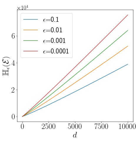
 

Refer to caption
Figure 4: We plot the rate-distortion upper bound from Theorem 23 for θ∼𝒩⁡(0,Id)\theta\sim\mathcal{N}(0,I_{d}) and W∼𝒩⁡(0,0.1)W\sim\mathcal{N}(0,0.1) as a function of the dimension dd for various levels of distortion ϵ\epsilon. The plots suggest that ℍϵ​(ℰ)=𝒪~​(d)\mathbb{H}_{\epsilon}(\mathcal{E})=\tilde{\mathcal{O}}(d) and that rate increases as the distortion decreases. Note that since the y-axis is in log scale, the graph also suggests that the rate-distortion function has a logarithmic dependence on 1ϵ\frac{1}{\epsilon}

.

Now, these results suggest the following sample complexity bounds for linear regression:

Theorem 26.

(subgaussian linear regression sample complexity bounds) For all d∈ℤ+⁣+d\in\mathbb{Z}_{++} s.t. d>2d>2, σ2≥0\sigma^{2}\geq 0, ϵ∈[0,12​(4​d+σ2)]\epsilon\in\left[0,\frac{1}{2(4d+\sigma^{2})}\right], and random vectors θ:Ω↦ℜd\theta:\Omega\mapsto\Re^{d} consisting of iid components that are each 11-subgaussian and symmetric, if for all tt, ℙ(Xt∈⋅)∼𝒩(0,Id)\mathbb{P}(X_{t}\in\cdot)\sim\mathcal{N}(0,I_{d}), and if for all x∈ℜdx\in\Re^{d}, ℰ(⋅|x)∼𝒩(θ⊤x,σ2)\mathcal{E}(\cdot|x)\sim\mathcal{N}(\theta^{\top}x,\sigma^{2}), then

d2​ϵ​ln⁡(d2​(4​d+σ2)​ϵ)≤Tϵ≤dϵ​ln⁡(dσ2​ϵ)\frac{d}{2\epsilon}\ln\left(\frac{d}{2(4d+\sigma^{2})\epsilon}\right)\ \leq\ T_{\epsilon}\ \leq\ \frac{d}{\epsilon}\ln\left(\frac{d}{\sigma^{2}\epsilon}\right)

Proof The result follows from Theorems 23, 25, and 15.  

6.3 Linear Regression with a Misspecified Model

In this section, we will study two instances of linear regression in which the model used by the agent is misspecified. We first study the case in which the agent’s prior over the environment has an incorrect mean. As one may expect, in this case, with enough data, the agent will still be able to arrive at the correct model. In the second instance, the agent’s prior will be missing a feature. In this instance, we will show that an irreducible error will linger even as T→∞T\rightarrow\infty.

Both of these instances will hinge upon the following result.

Corollary 27.

(misspecified/suboptimal prediction) For all t≥0t\geq 0 and π\pi,

𝔼[𝐝KL(Pt∗∥Pt)|Ht]=𝔼[𝐝KL(Pt∗∥P^t)|Ht]+𝔼[𝐝KL(P^t∥Pt)|Ht],\mathbb{E}[\mathbf{d}_{\mathrm{KL}}(P_{t}^{*}\|P_{t})\ |\ H_{t}]=\mathbb{E}[\mathbf{d}_{\mathrm{KL}}(P^{*}_{t}\|\hat{P}_{t})\ |\ H_{t}]+\mathbb{E}[\mathbf{d}_{\mathrm{KL}}(\hat{P}_{t}\|P_{t})\ |\ H_{t}],

where Pt=π⁡(Ht,Zt)P_{t}=\pi(H_{t},Z_{t}).

The first term on the RHS of Corollary 27 is the error of the correctly specified optimal learner. To study the shortfall, we will bound the behavior of the second term 𝔼[𝐝KL(P^t∥Pt)|Ht]\mathbb{E}[\mathbf{d}_{\mathrm{KL}}(\hat{P}_{t}\|P_{t})|H_{t}] in the two aforementioned problem instances. Proofs for these results may be found in Appendix B.

6.3.1 Prior with Incorrect Mean

Let the data generating process be the same as in Section 6.2. However, let the agent’s prior ℙ(θ∈⋅)∼𝒩(μ,Id)\mathbb{P}(\theta\in\cdot)\sim\mathcal{N}(\mu,I_{d}) for some μ∈ℜd\mu\in\Re^{d}. Note that when μ=0\mu=0 the prior is correctly specified. We will study the regret and sample complexity of this agent.

Theorem 28.

(incremental error of mean-misspecified agent) For all d,t∈ℤ+⁣+d,t\in\mathbb{Z}_{++} and μ∈ℜd\mu\in\Re^{d}, if t≥4​dt\geq 4d, then

𝔼[𝐝KL(P^t∥Pt)]≤d∥μ∥22(2t2+12​σ2e−(12​t−d)22),\mathbb{E}[\mathbf{d}_{\mathrm{KL}}(\hat{P}_{t}\|P_{t})]\leq d\|\mu\|_{2}^{2}\left(\frac{2}{t^{2}}+\frac{1}{2\sigma^{2}}e^{-\frac{\left(\frac{1}{2}\sqrt{t}-\sqrt{d}\right)^{2}}{2}}\right),

where PtP_{t} is the posterior distribution ℙ⁡(Yt+1|Ht)\mathbb{P}(Y_{t+1}|H_{t}) with misspecified prior ℙ⁡(θ)∼𝒩⁡(μ,Id)\mathbb{P}(\theta)\sim\mathcal{N}(\mu,I_{d}).

Refer to caption
Figure 5: Here we plot 𝔼[𝐝KL(Pt∗∥Pt)]\mathbb{E}[\mathbf{d}_{\mathrm{KL}}(P^{*}_{t}\|P_{t})] for the mean-misspecified agent using Corollary 27 and Theorem 28. We take d=100,σ2=0.01d=100,\sigma^{2}=0.01, and ‖μ‖22=1\|\mu\|^{2}_{2}=1. We observe that the error incurred by misspecification rapidly decays to 0.

The proof can be found in Appendix B. If we analyze Theorem 28 and Figure 5, we see that despite having a misspecified model, the excess error 𝔼[𝐝KL(P^t∥Pt)]\mathbb{E}[\mathbf{d}_{\mathrm{KL}}(\hat{P}_{t}\|P_{t})] goes to 00 at a rate of 1t2\frac{1}{t^{2}}. Also as expected, models with μ\mu larger in magnitude (and hence greater misspecification) require more samples to wash out. With Theorem 28 and similar techniques, one can derive regret/sample complexity bounds for suboptimal agents.

6.3.2 Prior with Missing Feature

We will now study another instance of misspecification under our framework for which the excess error does not decay to 00 as t→∞t\rightarrow\infty. Let the data generating process be the same as in Section 6.2. For i∈{1,…,d}i\in\{1,\ldots,d\}, let θi\theta_{i} denote the iith element of θ\theta. Let the agent’s prior be correctly specified for i∈{1,…,d−1}i\in\{1,\ldots,d-1\} (ℙ(θi∈⋅)∼𝒩(0,1)\mathbb{P}(\theta_{i}\in\cdot)\sim\mathcal{N}(0,1)), but suppose the final element’s prior is incorrectly ℙ(θd∈⋅)=𝟙[θd=0]\mathbb{P}(\theta_{d}\in\cdot)=\mathbbm{1}[\theta_{d}=0]. We will study the regret and sample complexity of this agent.

Theorem 29.

(incremental error of missing feature agent) For all d,t∈ℤ+⁣+d,t\in\mathbb{Z}_{++} and μ∈ℜd\mu\in\Re^{d}, if Pt​(Yt|Ht)P_{t}(Y_{t}|H_{t}) is the postersior distribution of YtY_{t} conditioned on HtH_{t} with the incorrect prior ℙ(θd∈⋅)∼𝟙[θd=0]\mathbb{P}(\theta_{d}\in\cdot)\sim\mathbbm{1}[\theta_{d}=0], then

limt→∞𝔼[𝐝KL(P^t∥Pt)]=12𝔼[ln(1+Xt,d2σ2)],\lim_{t\rightarrow\infty}\mathbb{E}\left[\mathbf{d}_{\mathrm{KL}}(\hat{P}_{t}\|P_{t})\right]=\frac{1}{2}\mathbb{E}\left[\ln\left(1+\frac{X^{2}_{t,d}}{\sigma^{2}}\right)\right],

where Xt,dX_{t,d} denotes the ddth component of XtX_{t}.

Theorem 29 suggests that for an agent that is oblivious to one of the features, the incremental error will never go below 12​𝔼​[ln⁡(1+Xt,d2σ2)]\frac{1}{2}\mathbb{E}\left[\ln\left(1+\frac{X^{2}_{t,d}}{\sigma^{2}}\right)\right] in expectation. This is intuitive as the true label YY depends on the omitted feature. By ignoring that feature, the agent always leaves a bit of performance at the table.

7 Deep Neural Network Environments

In this section, we will focus on characterizing the rate-distortion function, and hence the sample complexity, of different deep neural network environments. As seen in the previous section, for the analysis of rate-distortion, it suffices to restrict attention to a representative input-output pair rather than a sequence, i.e., the distortion depends on one representative input-output pair and not the sequence ((Xt,Yt+1):t∈ℤ+)((X_{t},Y_{t+1}):t\in\mathbb{Z}_{+}). We will denote this representative pair by (X,Y)(X,Y). The input XX is distributed ℙ(X∈⋅)∼𝒩(0,I)\mathbb{P}(X\in\cdot)\sim\mathcal{N}(0,I), while the conditional distribution of the output is ℙ(Y∈⋅|ℰ,X)=ℰ(⋅|X)\mathbb{P}(Y\in\cdot|\mathcal{E},X)=\mathcal{E}(\cdot|X).

For environments we consider in this section, XX takes values in ℜd\Re^{d} and YY take values in ℜ\Re, and Y=f⁡(X)+WY=f(X)+W for a random function ff and random variable W∼𝒩⁡(0,σ2​Id)W\sim\mathcal{N}(0,\sigma^{2}I_{d}). We assume XX, ff, and WW are independent. The environment is produced by composing KK independent and identically distributed random functions: f=fK∘⋯∘f1f=f_{K}\circ\cdots\circ f_{1}. In this sense, the environment is multilayer, with each kkth layer represented by a function fkf_{k}. We denote inputs and outputs of these functions by U0=XU_{0}=X and Uk=fk​(Uk−1)U_{k}=f_{k}(U_{k-1}) for k=1,…,Kk=1,\ldots,K. Hence, Y=UK+WY=U_{K}+W. Figure 6 illustrates the structure of such an environment.

Figure 6: A multilayer environment.

Our analysis will relate the rate-distortion function ℍϵ​(ℰ)\mathbb{H}_{\epsilon}(\mathcal{E}) of the multilayer environment to that of KK single-layer environments. Each such single-layer environment, which we denote by ℰk\mathcal{E}_{k}, takes the form ℰk(⋅|u)∼𝒩(fk(u),σ2Id)\mathcal{E}_{k}(\cdot|u)\sim\mathcal{N}(f_{k}(u),\sigma^{2}I_{d}). In other words, conditioned on ℰk\mathcal{E}_{k} and the input Uk−1U_{k-1}, the output of ℰk\mathcal{E}_{k} is distributed according to Uk+WU_{k}+W.

To frame our our results, we define a class of proxies that decompose independently accross layers. Recall that an environment proxy of an environment ℰ\mathcal{E} is a random variable ℰ~\tilde{\mathcal{E}} for which ℰ~⟂H∞|ℰ\tilde{\mathcal{E}}\perp H_{\infty}|\mathcal{E}. Similarly, an environment proxy of ℰk\mathcal{E}_{k} is a random variable ℰ~k\tilde{\mathcal{E}}_{k} for which ℰ~k⟂H∞|ℰk\tilde{\mathcal{E}}_{k}\perp H_{\infty}|\mathcal{E}_{k}. This definition allows for dependence between the proxies across layers even though we have assumed environments to be iid across layers. To restrict attention to independent single-layer proxies, we define a multilayer proxy to be a tuple ℰ~=(ℰ~1,…,ℰ~K)\tilde{\mathcal{E}}=(\tilde{\mathcal{E}}_{1},\ldots,\tilde{\mathcal{E}}_{K}) such that ℰ~k⟂(ℰ¬k,ℰ~¬k,H∞)|ℰk\tilde{\mathcal{E}}_{k}\perp(\mathcal{E}_{\lnot k},\tilde{\mathcal{E}}_{\lnot k},H_{\infty})|\mathcal{E}_{k}, where ℰ¬k\mathcal{E}_{\lnot k} and ℰ~¬k\tilde{\mathcal{E}}_{\lnot k} denote tuples of single-layer environments and proxies, with the kkth omitted.

7.1 Prototypical Neural Network Environment

In this section, we present two multilayer neural network environment for which we will eventually study the sample complexity of. We will see that the choice of prior will influence the types of bounds that are possible to derive. We hope that these examples give the reader a wide enough breadth of techniques to analyze their own interesting multilayer environments.

Figure 7: Prototypical Neural Network Environment

Our first prototypical neural network environment mirrors is a fully-connected feed-forward neural network with ReLU activations (Figure 7). Let

U1=f1​(U0)=ReLU⁡(A(1)​U0),U_{1}=f_{1}(U_{0})={\rm ReLU}(A^{(1)}U_{0}),

where A(1)∈ℜN×dA^{(1)}\in\Re^{N\times d}. For k∈{2,…,K−1}k\in\{2,\ldots,K-1\}, let

Uk=fk​(Uk−1)=ReLU⁡(A(k)​Uk−1),U_{k}=f_{k}(U_{k-1})={\rm ReLU}(A^{(k)}U_{k-1}),

where A(k)∈ℜN×N∈ℜNA^{(k)}\in\Re^{N\times N}\in\Re^{N}. For the final layer, let

UK=fK​(UK−1)=A(K)⊤​UK−1,U_{K}=f_{K}(U_{K-1})=A^{(K)\top}U_{K-1},

where A(K)∈ℜNA^{(K)}\in\Re^{N}. In this environment, ℰk\mathcal{E}_{k} is identified by (A(k))(A^{(k)}) for k∈{1,…,K−1}k\in\{1,\ldots,K-1\} and ℰK\mathcal{E}_{K} is identified by A(K)A^{(K)}.

Note that this model can trivially incorporate biases by appending a dimension to UiU_{i} that is constant with value 11. All results in this paper can incorporate this extension as well but we use the above formulation for notational simplicity. We will now introduce a prior distribution on the weight matrices that we will analyze.

7.2 Independent Prior

The first prior distribution we consider involves weights that are independent from one another. Formally:

∀k∈{1,…,K},Ai,j(k)⟂Al,m(k)​ for ​(i,j)≠(l,m).\forall k\in\{1,\ldots,K\},\quad A^{(k)}_{i,j}\perp A^{(k)}_{l,m}\text{ for }(i,j)\neq(l,m).

Furthermore, for normalization purposes, we impose the following further constraints:

∀k∈{1,…,K},𝔼⁡[Ai,j(k)]=0;𝕍⁡[Ai,j(k)]={1d,if ​k=11N,if ​k≠1}.\forall k\in\{1,\ldots,K\},\quad\mathbb{E}\left[A_{i,j}^{(k)}\right]=0;\quad\mathbb{V}\left[A_{i,j}^{(k)}\right]=\left\{\begin{array}[]{lr}\frac{1}{d},&\text{if }k=1\\ \frac{1}{N},&\text{if }k\neq 1\end{array}\right\}.

We will refer to this prior as the independent prior since each weight in the neural network is independent.

7.3 Dirichlet Prior

Figure 8: Dirichlet weights neural network environment. We let dd denote the input dimension, KK denote the depth, and NN denote the (potentially infinite) width. Note that despite the infinite width, structure is assumed via a Dirichlet prior which induces a sparsity-like effect.

The other distribution we will consider is the following. Each layer kk consists of two matrices: A(k)∈ℜM×d,B(k)∈ℜd×MA^{(k)}\in\Re^{M\times d},B^{(k)}\in\Re^{d\times M}. For all k∈{1,…,K}k\in\{1,\ldots,K\},

A(k)=[−A1(k)⊤−−AM(k)⊤−],A^{(k)}=\begin{bmatrix}-&A_{1}^{(k)\top}&-\\ \vdots&\vdots&\vdots\\ -&A_{M}^{(k)\top}&-\\ \end{bmatrix},

where for all ii, Ai(k)∼𝒩⁡(0,Id/d)A_{i}^{(k)}\sim\mathcal{N}(0,I_{d}/d). Meanwhile, for all k∈{1,…,K−1}k\in\{1,\ldots,K-1\}

B(k)=[−M​B1(k)⊤−−M​Bd(k)⊤−],B^{(k)}=\begin{bmatrix}-&\sqrt{M}B_{1}^{(k)\top}&-\\ \vdots&\vdots&\vdots\\ -&\sqrt{M}B_{d}^{(k)\top}&-\\ \end{bmatrix},

where for all ii, B¯i(k)∼Dirichlet⁡(M/N,…,M/N)\bar{B}_{i}^{(k)}\sim{\rm Dirichlet}(M/N,\ldots,M/N) and

Bi(k)={B¯i(k)w.p. ​0.5−B¯i(k)w.p. ​0.5.B_{i}^{(k)}=\begin{cases}\bar{B}_{i}^{(k)}&\text{w.p. }0.5\\ -\bar{B}_{i}^{(k)}&\text{w.p. }0.5\\ \end{cases}.

Meanwhile, we let B(K)∈ℜNB^{(K)}\in\Re^{N} have output dimension 11. B(K)B^{(K)} is also distributed Dirichlet with the same parameters. For all k∈{1,…,K−1}k\in\{1,\ldots,K-1\}, conditioned on A(k)A^{(k)} and B(k)B^{(k)}, we have that

Uk=ReLU⁡(B(k)​ReLU​(A(k)​Uk−1)).U_{k}={\rm ReLU}(B^{(k)}{\rm ReLU}(A^{(k)}U_{k-1})).

Finally, for the output layer, we have that

UK=B(K)⊤​ReLU​(A(K)​UK−1).U_{K}=B^{(K)\top}{\rm ReLU}(A^{(K)}U_{K-1}).

For this prior, we will assume that M≪NM\ll N. We will refer to this prior as the dirichlet prior. This data generating process is effectively nonparametric, as NN can be taken to be arbitrarily large. We will show that despite this, the complexity of the environment is bounded by the scale parameter MM and entirely independent of the width of the network (N)(N). In the following section, we will formalize the above by deriving single-layer rate-distortion bounds that are independent of the width NN.

7.4 Width-Independence in Rate Distortion Bounds

In this section, we demonstrate that the prior on the weights of the network can dramatically impact the rate-distortion function of a single layer. Notably, we can derive rate-distortion bounds that are dictated mainly by matrix norms and are width independent. This is an important characteristic that researchers have been exploring i.e moving beyond parameter-count based bounds to better explain the empirical behavior of large-scale neural networks which may be very wide. Proofs may be found in Appendix C

We begin by presenting a simple parameter-count based rate-distortion bound for a single-layer relu neural network.

Theorem 30.

(independent single-layer rate-distortion bound) For all d,N∈ℤ+⁣+d,N\in\mathbb{Z}_{++} and σ2,ϵ≥0\sigma^{2},\epsilon\geq 0, if ℰ\mathcal{E} is a single-layer neural network with the independent prior, then

ℍϵ​(ℰ)≤d​N2​ln⁡(N2​σ2​ϵ).\mathbb{H}_{\epsilon}(\mathcal{E})\leq\frac{dN}{2}\ln\left(\frac{N}{2\sigma^{2}\epsilon}\right).

With the independent prior, we cannot escape the linear width NN dependence in the rate-distortion function. However, when we consider different priors with dependence between weights, for example the dirichlet prior, we can provide a rate-distortion bound that is independent of NN.

Theorem 31.

(dirichlet single-layer rate-distortion bound) For all d,M,N∈ℤ+⁣+d,M,N\in\mathbb{Z}_{++} and σ2,ϵ≥0\sigma^{2},\epsilon\geq 0, if ℰ\mathcal{E} is a single-layer neural network environment with the dirichlet prior, then

ℍϵ​(ℰ)≤d2​M​ln2⁡(3​dσ2​ϵ).\mathbb{H}_{\epsilon}(\mathcal{E})\leq d^{2}M\ln^{2}\left(\frac{3d}{\sigma^{2}\epsilon}\right).

The rate-distortion bound is able to capture the fact that while NN could be infinite, the sparsity-like effect induced by the dirichlet prior fundamentally limits the complexity of learning. The bound instead depends only linearly on d2d^{2}, MM and logarithmically in the tolerance ϵ\epsilon.

7.5 Avoiding Width Dependence with only Linear Depth Dependence

While the flavor of results in section 7.4 have been heavily studied, a shortcoming of these results is that when adapting width-independent bounds to deep neural networks, the eventual sample complexity becomes exponential in the depth. Meanwhile classical VC-dimension parameter count results provide sample complexity bounds that are 𝒪⁡(K2​N)\mathcal{O}(K^{2}N) where KK and NN are the depth and width respectively. While the depth dependence is much better than exponential, the width dependence is considered problematic by the research community.

A sample complexity bound that simultaneously provides good depth and width dependence has been illusive. While there are results such as those of Wei and Ma 2019 which provide “polynomial” dependence on depth and input dimension, further dependence is hidden in so-called data-dependent quantities that are difficult to analyze and understand. Furthermore even high-order polynomial dependence on depth and width are prohibitive in the regime of modern deep learning.

7.6 Decomposing the Error of Multilayer Environments

In this section, we provide sample complexity bounds that exhibit both favorable depth and width dependence. We are able to achieve this by leveraging an average-case framework and information-theoretic tools.

Figure 9: The error incurred by a multilayer proxy ℰ~K:1\tilde{\mathcal{E}}_{K:1} measures the difference between true output YY and the prediction Y~\tilde{Y} (shown in red box). This difference is the result of error that builds up through layers of the environment (denoted by red dotted outline).

For multilayer environments, it becomes apparent that error is more cumbersome to reason about. Figure 9 depicts the error incurred by using a multilayer proxy ℰK:1\mathcal{E}_{K:1} to approximate multilayer environment ℰK:1\mathcal{E}_{K:1}. Evidently, it seems tricky to reason about the error propagation through the layers of the environment. Many existing lines of analysis struggle on this front and result in sample complexity bounds that are exponential in the depth of the network Bartlett et al. 2017, Golowich et al. 2018. The techniques in these papers consider a worst-case reasoning under which an ϵ\epsilon error between the first outputs U1U_{1} and U~1\tilde{U}_{1} may blow up to a λK​ϵ\lambda^{K}\epsilon error when passed through remaining layers of the network (where λ\lambda is a spectral radius).

Figure 10: A much easier system to analyze is one in which we measure the incremental error at each stage of the multilayer environment. If each layer incurs an error of ϵK\frac{\epsilon}{K}, the total error incurred will be ϵ\epsilon. Note that the inputs to each layer are correctly specified in this system. We show that in many cases, analyzing the error of this system upper bounds the error of the system in Figure 9.

It would be much simpler to instead independently analyze the incremental error incurred at each stage of the network. Figure 10 depicts this. We consider that at each layer, we know the true input Uk−1U_{k-1} and simply measure the immediate error incurred at the output UkU_{k} as opposed to the error incurred at the final output of the network YY.

Mathematically, the error incurred by the full system from using proxy ℰ~K:1\tilde{\mathcal{E}}_{K:1} can be expressed as 𝕀(Y;ℰK:1|ℰ~K:1,X)\mathbb{I}(Y;\mathcal{E}_{K:1}|\tilde{\mathcal{E}}_{K:1},X). By the chain rule, this error decomposes into:

𝕀(Y;ℰK:1|ℰ~K:1,X)=∑k=1K𝕀(Y;ℰk|ℰK:k+1,ℰ~k:1,X).\mathbb{I}(Y;\mathcal{E}_{K:1}|\tilde{\mathcal{E}}_{K:1},X)=\sum_{k=1}^{K}\mathbb{I}(Y;\mathcal{E}_{k}|\mathcal{E}_{K:k+1},\tilde{\mathcal{E}}_{k:1},X). (2)

Therefore, the error incurred from layer kk can be expressed as 𝕀(Y;ℰk|ℰK:k+1,ℰ~k:1,X)\mathbb{I}(Y;\mathcal{E}_{k}|\mathcal{E}_{K:k+1},\tilde{\mathcal{E}}_{k:1},X). This is cumbersome as we are not given the true input Uk−1U_{k-1} but rather an approximation from input XX and ℰ~k−1:1\tilde{\mathcal{E}}_{k-1:1}. Furthermore, we are measuring the error in the final output YY as opposed to the immediate output UkU_{k}. It would be much more simple to analyze something like the following:

∑k=1K𝕀(Uk+W;ℰk|ℰ~k,Uk−1),\sum_{k=1}^{K}\mathbb{I}(U_{k}+W;\mathcal{E}_{k}|\tilde{\mathcal{E}}_{k},U_{k-1}), (3)

where WW is independent 00-mean gaussian noise with variance σ2\sigma^{2} in each dimension. This sum is much easier to work with because the kkth term only depends on ℰk,ℰ~k,Uk−1,\mathcal{E}_{k},\tilde{\mathcal{E}}_{k},U_{k-1}, and UkU_{k}. There is no inter-layer dependence.

7.6.1 Sufficient Conditions to Avoid Inter-Layer Dependence

The key insight is that in our deep neural network environment, something akin to the following will hold:

𝕀(Y;ℰk|ℰK:k+1,ℰ~k:1,X)≤𝕀(Uk+W;ℰk|ℰ~k,Uk−1).\mathbb{I}(Y;\mathcal{E}_{k}|\mathcal{E}_{K:k+1},\tilde{\mathcal{E}}_{k:1},X)\leq\mathbb{I}(U_{k}+W;\mathcal{E}_{k}|\tilde{\mathcal{E}}_{k},U_{k-1}). (4)

As a result, the cumbersome sum 2 will be upper bounded by the amenable sum 3.

The condition in inequality 4 involves two parts:

  1. 1.

    𝕀(Y;ℰk|ℰK:k+1,ℰ~k:1,X)≤𝕀(Y;ℰk|ℰK:k+1,ℰ~k,Uk−1)\mathbb{I}(Y;\mathcal{E}_{k}|\mathcal{E}_{K:k+1},\tilde{\mathcal{E}}_{k:1},X)\leq\mathbb{I}(Y;\mathcal{E}_{k}|\mathcal{E}_{K:k+1},\tilde{\mathcal{E}}_{k},U_{k-1})

    • •

      Conditioning on the true input Uk−1U_{k-1} provides more information about ℰk\mathcal{E}_{k} than conditioning on an approximation (ℰ~k−1:1,X)(\tilde{\mathcal{E}}_{k-1:1},X).

  2. 2.

    𝕀(Y;ℰk|ℰK:k+1,ℰ~k,Uk−1)≤𝕀(Uk+W;ℰk|ℰ~k,Uk−1)\mathbb{I}(Y;\mathcal{E}_{k}|\mathcal{E}_{K:k+1},\tilde{\mathcal{E}}_{k},U_{k-1})\leq\mathbb{I}(U_{k}+W;\mathcal{E}_{k}|\tilde{\mathcal{E}}_{k},U_{k-1})

    • •

      The immediate output Uk+WU_{k}+W provides more information about ℰk\mathcal{E}_{k} than the final output YY does.

OPEN1)1) holds for all proxies of the form ℰ~=(ℰ~1,…,ℰ~K)\tilde{\mathcal{E}}=(\tilde{\mathcal{E}}_{1},\ldots,\tilde{\mathcal{E}}_{K}) where ℰ~i⟂ℰ~j\tilde{\mathcal{E}}_{i}\perp\tilde{\mathcal{E}}_{j} for i≠ji\neq j. We prove this result explicitly in Lemma 33. It is rather intuitive that the pristine data pair (Uk−1,Y)(U_{k-1},Y) would provide more information about ℰk\mathcal{E}_{k} than (U0,ℰ~k−1:1,Y)(U_{0},\tilde{\mathcal{E}}_{k-1:1},Y) would as some information ought to be lost through the imperfect reconstruction of Uk−1U_{k-1} from U0U_{0} and ℰ~k−1:1\tilde{\mathcal{E}}_{k-1:1}.

OPEN2)2) will not hold exactly for our environments. However, a slightly modified result of similar spirit will be shown. 𝕀(Y;ℰk|ℰK:k+1,Uk−1)\mathbb{I}(Y;\mathcal{E}_{k}|\mathcal{E}_{K:k+1},U_{k-1}) will be ≤\leq an upper bound of 𝕀(Uk+W,ℰk|ℰk,Uk−1)\mathbb{I}(U_{k}+W,\mathcal{E}_{k}|\mathcal{E}_{k},U_{k-1}) which was already used to upper bound the distortion function in the single-layer results. We leave the details to Lemma 37.

The impact of inequality 4 on the eventual sample-complexity bounds can be seen through the following result:

Lemma 32.

If ℰK:1\mathcal{E}_{K:1} is such that for all k∈[K]k\in[K] and multilayer-proxies ℰ~=(ℰ~1,…,ℰ~K)\tilde{\mathcal{E}}=(\tilde{\mathcal{E}}_{1},\ldots,\tilde{\mathcal{E}}_{K}),

𝕀(Y;ℰk|ℰK:k+1,ℰ~k,Uk−1)≤𝕀(Uk+W;ℰk|ℰ~k,Uk−1),\mathbb{I}(Y;\mathcal{E}_{k}|\mathcal{E}_{K:k+1},\tilde{\mathcal{E}}_{k},U_{k-1})\leq\mathbb{I}(U_{k}+W;\mathcal{E}_{k}|\tilde{\mathcal{E}}_{k},U_{k-1}),

then for all ϵ≥0\epsilon\geq 0,

ℍϵ(ℰK:1)≤∑k=1KℍϵK(ℰk).\mathbb{H}_{\epsilon}(\mathcal{E}_{K:1})\leq\sum_{k=1}^{K}\mathbb{H}_{\frac{\epsilon}{K}}(\mathcal{E}_{k}).

This result suggests that the rate-distortion (and hence sample complexity) of the full multilayer system is linear in the depth KK and the rate-distortion function of the single layer environment at distortion level ϵK\frac{\epsilon}{K}. Since in section 7.4, we established that the single-layer rate-distortion function had favorable width dependence and at most logarithmic dependence on 1ϵ\frac{1}{\epsilon}, we are able to (and eventually will) establish sample complexity bounds that simultaneously exhibit negligible width dependence and at most quadratic depth dependence.

7.7 Establishing the Conditions for Favorable Depth Dependence

In this section, we formally prove the properties from section 7.6.1 in the context of our prototypical neural network environment. We begin by establishing property OPEN1)1).

Lemma 33.

(more is learned with the true input) Let ℰ~K:1\tilde{\mathcal{E}}_{K:1} be a multilayer proxy. Then, for all k∈{1,…,K}k\in\{1,\ldots,K\},

𝕀(Y;ℰk|ℰK:k+1,ℰ~k:1,X)≤𝕀(Y;ℰk|ℰK:k+1,ℰ~k,Uk−1).\mathbb{I}(Y;\mathcal{E}_{k}|\mathcal{E}_{K:k+1},\tilde{\mathcal{E}}_{k:1},X)\leq\mathbb{I}(Y;\mathcal{E}_{k}|\mathcal{E}_{K:k+1},\tilde{\mathcal{E}}_{k},U_{k-1}).

Proof

𝕀(ℰk;Y|ℰK:k+1,ℰ~k:1,X)\displaystyle\mathbb{I}(\mathcal{E}_{k};Y|\mathcal{E}_{K:k+1},\tilde{\mathcal{E}}_{k:1},X)
=𝕀(ℰk;ℰ~k−1:1,X,Y|ℰK:k+1,ℰ~k)−𝕀(ℰk;ℰ~k−1:1,X|ℰK:k+1,ℰ~k)\displaystyle=\mathbb{I}(\mathcal{E}_{k};\tilde{\mathcal{E}}_{k-1:1},X,Y|\mathcal{E}_{K:k+1},\tilde{\mathcal{E}}_{k})-\mathbb{I}(\mathcal{E}_{k};\tilde{\mathcal{E}}_{k-1:1},X|\mathcal{E}_{K:k+1},\tilde{\mathcal{E}}_{k})
=𝕀(ℰk;ℰ~j−1:1,X,Y|ℰK:k+1,ℰ~k)\displaystyle=\mathbb{I}(\mathcal{E}_{k};\tilde{\mathcal{E}}_{j-1:1},X,Y|\mathcal{E}_{K:k+1},\tilde{\mathcal{E}}_{k})
=𝕀(ℰk;Y|ℰK:k+1,ℰ~k)+𝕀(ℰk;ℰ~k−1:1,X|ℰK:k+1,ℰ~k,Y)\displaystyle=\mathbb{I}(\mathcal{E}_{k};Y|\mathcal{E}_{K:k+1},\tilde{\mathcal{E}}_{k})+\mathbb{I}(\mathcal{E}_{k};\tilde{\mathcal{E}}_{k-1:1},X|\mathcal{E}_{K:k+1},\tilde{\mathcal{E}}_{k},Y)
≤(a)𝕀(ℰk;Y|ℰK:k+1,ℰ~k)+𝕀(ℰk;ℰk−1:1,X|ℰK:k+1,ℰ~k,Y)\displaystyle\overset{(a)}{\leq}\mathbb{I}(\mathcal{E}_{k};Y|\mathcal{E}_{K:k+1},\tilde{\mathcal{E}}_{k})+\mathbb{I}(\mathcal{E}_{k};\mathcal{E}_{k-1:1},X|\mathcal{E}_{K:k+1},\tilde{\mathcal{E}}_{k},Y)
=𝕀(ℰk;ℰk−1,1,X,Y|ℰK:k+1,ℰ~k)\displaystyle=\mathbb{I}(\mathcal{E}_{k};\mathcal{E}_{k-1,1},X,Y|\mathcal{E}_{K:k+1},\tilde{\mathcal{E}}_{k})
=(b)𝕀(ℰk;Y|ℰK:k+1,ℰ~k,ℰk−1:1,X)\displaystyle\overset{(b)}{=}\mathbb{I}(\mathcal{E}_{k};Y|\mathcal{E}_{K:k+1},\tilde{\mathcal{E}}_{k},\mathcal{E}_{k-1:1},X)
=(c)𝕀(ℰk;Y|ℰK:k+1,ℰ~k,Uk−1),\displaystyle\overset{(c)}{=}\mathbb{I}(\mathcal{E}_{k};Y|\mathcal{E}_{K:k+1},\tilde{\mathcal{E}}_{k},U_{k-1}),

where (a)(a) follows from the fact that ℰk⟂ℰ~k−1:1|(X,Y,ℰk−1:1)\mathcal{E}_{k}\perp\tilde{\mathcal{E}}_{k-1:1}|(X,Y,\mathcal{E}_{k-1:1}) and the data processing inequality, (b)(b) follows from the fact that 𝕀(ℰk;ℰk−1:1,X|ℰK:k+1,ℰ~k)=0\mathbb{I}(\mathcal{E}_{k};\mathcal{E}_{k-1:1},X|\mathcal{E}_{K:k+1},\tilde{\mathcal{E}}_{k})=0, and (c)(c) follows from the fact that Y⟂(ℰk−1:1,X)|Uk−1Y\perp(\mathcal{E}_{k-1:1},X)|U_{k-1}.  

Lemma 33 states that we learn more information about ℰk\mathcal{E}_{k} when we are given the true input Uk−1U_{k-1} than when we are given (X,ℰ~k−1:1)(X,\tilde{\mathcal{E}}_{k-1:1}) and have to infer Uk−1U_{k-1}. This is intuitive as we should be able to recover more about ℰk\mathcal{E}_{k} when we observe its input exactly.

We now show a suitable alternative to property OPEN2)2). Intuitively, the immediate output Uk+WU_{k}+W will provide more information about ℰk\mathcal{E}_{k} than the final output YY so long as in expectation, the layers fk+1,…,fKf_{k+1},\ldots,f_{K} don’t amplify the scale of the output. If they were to amplify the scale, then the signal to noise ratio of YY would look larger than that of Uk+WU_{k}+W, leading to potentially more information. To express this idea mathematically, our results will rely on the following quantity for each layer k∈[K]k\in[K]:

L(k)=supx,y𝔼[‖f(k)​(x)−f(k)​(y)‖22‖x−y‖22|x=x,y=y].L^{(k)}=\sup_{x,y}\mathbb{E}\left[\frac{\|f^{(k)}(x)-f^{(k)}(y)\|^{2}_{2}}{\|x-y\|^{2}_{2}}\Big|x=x,y=y\right].

L(k)L^{(k)} is the expected squared lipschitz constant (averaged over the randomness in f(k)f^{(k)}) of the function at layer kk. So long as the product ∏i=kKL(i)≤1\prod_{i=k}^{K}L^{(i)}\leq 1 for each k∈[K]k\in[K], we will effectively have property OPEN2)2).

The following result expresses LL concretely for a single layer of the prototypical neural network we study in this work.

Lemma 34.

(relu neural network layer stability) For all N,M∈ℤ+⁣+N,M\in\mathbb{Z}_{++}, if A∈ℜM×NA\in\Re^{M\times N} is a random matrix and f⁡(x)=ReLU⁡(A​x)f(x)={\rm ReLU}(Ax) for x∈ℜNx\in\Re^{N}, then

L=supx,y∈ℜN𝔼[‖f⁡(x)−f⁡(y)‖22‖x−y‖22|x=x,y=y]=‖𝔼[A⊤A]‖σ,L=\sup_{x,y\in\Re^{N}}\mathbb{E}\left[\frac{\|f(x)-f(y)\|^{2}_{2}}{\|x-y\|^{2}_{2}}\Big|x=x,y=y\right]=\left\|\mathbb{E}\left[A^{\top}A\right]\right\|_{\sigma},

where ∥⋅∥σ\|\cdot\|_{\sigma} denotes the operator norm.

Proof

L\displaystyle L =supx,y∈ℜN𝔼[‖f⁡(x)−f⁡(y)‖22‖x−y‖22|x=x,y=y]\displaystyle=\sup_{x,y\in\Re^{N}}\mathbb{E}\left[\frac{\|f(x)-f(y)\|^{2}_{2}}{\|x-y\|^{2}_{2}}\Big|x=x,y=y\right]
=supx,y∈ℜN𝔼[‖ReLU⁡(A​x)−ReLU⁡(A​y)‖22‖x−y‖22|x=x,y=y]\displaystyle=\sup_{x,y\in\Re^{N}}\mathbb{E}\left[\frac{\|{\rm ReLU}(Ax)-{\rm ReLU}(Ay)\|^{2}_{2}}{\|x-y\|^{2}_{2}}\Big|x=x,y=y\right]
≤(a)supx,y∈ℜN𝔼[‖A⁡(x−y)‖22‖x−y‖22|x=x,y=y]\displaystyle\overset{(a)}{\leq}\sup_{x,y\in\Re^{N}}\mathbb{E}\left[\frac{\|A(x-y)\|^{2}_{2}}{\|x-y\|^{2}_{2}}\Big|x=x,y=y\right]
=supx,y∈ℜN𝔼[(x−y)⊤​A⊤​A​(x−y)‖x−y‖22|x=x,y=y]\displaystyle=\sup_{x,y\in\Re^{N}}\mathbb{E}\left[\frac{(x-y)^{\top}A^{\top}A(x-y)}{\|x-y\|^{2}_{2}}\Big|x=x,y=y\right]
=supx,y∈ℜN(x−y)⊤​𝔼​[A⊤​A]​(x−y)‖x−y‖22\displaystyle=\sup_{x,y\in\Re^{N}}\frac{(x-y)^{\top}\mathbb{E}\left[A^{\top}A\right](x-y)}{\|x-y\|^{2}_{2}}
=‖𝔼⁡[A⊤​A]‖σ,\displaystyle=\left\|\mathbb{E}\left[A^{\top}A\right]\right\|_{\sigma},

where (a)(a) follows from the fact that for all xx and yy, (ReLU⁡(x)−ReLU⁡(y))2≤(x−y)2({\rm ReLU}(x)-{\rm ReLU}(y))^{2}\leq(x-y)^{2}.  

Evidently LL will depend on the data generating process’s weight distribution. For independent prior, we have the following upper bound for LL:

Lemma 35.

(independent stability) For all di​n,do​u​t∈ℤ+⁣+d_{in},d_{out}\in\mathbb{Z}_{++}, if random matrix A∈ℜdo​u​t×di​nA\in\Re^{d_{out}\times d_{in}} consists of independent elements with mean 00 and variance 1di​n\frac{1}{d_{in}} and f⁡(X)=ReLU⁡(A​X)f(X)={\rm ReLU}(AX) for X∈ℜdi​nX\in\Re^{d_{in}}, then

L=supx,y∈ℜdi​n𝔼[‖f⁡(x)−f⁡(y)‖22‖x−y‖22|x=x,y=y]≤do​u​tdi​n.L=\sup_{x,y\in\Re^{d_{in}}}\mathbb{E}\left[\frac{\|f(x)-f(y)\|^{2}_{2}}{\|x-y\|^{2}_{2}}\Big|x=x,y=y\right]\leq\frac{d_{out}}{d_{in}}.

Proof

L\displaystyle L =(a)​‖𝔼⁡[A⊤​A]‖σ\displaystyle\overset{(a)}{=}\left\|\mathbb{E}\left[A^{\top}A\right]\right\|_{\sigma}
=‖do​u​tdi​n​Idi​n‖σ\displaystyle=\left\|\frac{d_{out}}{d_{in}}I_{d_{in}}\right\|_{\sigma}
=do​u​tdi​n,\displaystyle=\frac{d_{out}}{d_{in}},

where (a)(a) follows from Lemma 34.  

Meanwhile, for the dirichlet prior, we have the following result:

Lemma 36.

(dirichlet stability) For all N,M,di​n,do​u​t∈ℤ+⁣+N,M,d_{in},d_{out}\in\mathbb{Z}_{++}, if random matrices (A∈ℜN×di​n,B∈ℜdo​u​t,N)(A\in\Re^{N\times d_{in}},B\in\Re^{d_{out},N}) are distributed according to the dirichlet prior with M≤NM\leq\sqrt{N} and f⁡(X)=ReLU⁡(B​ReLU​(A​X))f(X)={\rm ReLU}(B\ {\rm ReLU}(AX)), then

L=supx,y∈ℜN𝔼[‖f⁡(x)−f⁡(y)‖22‖x−y‖22|x=x,y=y]≤do​u​tdi​n.L=\sup_{x,y\in\Re^{N}}\mathbb{E}\left[\frac{\|f(x)-f(y)\|^{2}_{2}}{\|x-y\|^{2}_{2}}\Big|x=x,y=y\right]\leq\frac{d_{out}}{d_{in}}.

Proof

L\displaystyle L ≤(a)​‖𝔼⁡[(A​B)⊤​(A​B)]‖σ\displaystyle\overset{(a)}{\leq}\left\|\mathbb{E}\left[(AB)^{\top}(AB)\right]\right\|_{\sigma}
=​‖𝔼⁡[A⊤​(do​u​t​M​(N+M)(M+1)​N2​IM)​A]‖σ\displaystyle\overset{}{=}\left\|\mathbb{E}\left[A^{\top}\left(\frac{d_{out}M(N+M)}{(M+1)N^{2}}I_{M}\right)A\right]\right\|_{\sigma}
=​(do​u​t​M​(N+M)(M+1)​N2​IM)​‖𝔼⁡[A⊤​A]‖σ\displaystyle\overset{}{=}\left(\frac{d_{out}M(N+M)}{(M+1)N^{2}}I_{M}\right)\left\|\mathbb{E}\left[A^{\top}A\right]\right\|_{\sigma}
=​(do​u​t​M​(N+M)(M+1)​N2​IM)​‖Ndi​n​Idi​n‖σ\displaystyle\overset{}{=}\left(\frac{d_{out}M(N+M)}{(M+1)N^{2}}I_{M}\right)\left\|\frac{N}{d_{in}}I_{d_{in}}\right\|_{\sigma}
=do​u​tdi​n​MM+1​N+MN\displaystyle=\frac{d_{out}}{d_{in}}\frac{M}{M+1}\frac{N+M}{N}
≤(b)​do​u​tdi​n,\displaystyle\overset{(b)}{\leq}\frac{d_{out}}{d_{in}},

where (a)(a) follows from the fact that for all xx and yy, (ReLU⁡(x)−ReLU⁡(y))2≤(x−y)2({\rm ReLU}(x)-{\rm ReLU}(y))^{2}\leq(x-y)^{2} and Lemma 34, and (b)(b) follows from the fact that M≤NM\leq\sqrt{N}.  

Since we assume that M≪NM\ll N, the above condition will hold for the data generating processes we are interested in. With these results in place, we now present a general bound for the distortion 𝕀(Y;ℰk|ℰ~k,ℰK:k+1,Uk−1)\mathbb{I}(Y;\mathcal{E}_{k}|\tilde{\mathcal{E}}_{k},\mathcal{E}_{K:k+1},U_{k-1}) in a multilayer environment.

Lemma 37.

(multilayer distortion bound) For all k,K∈ℤ+⁣+k,K\in\mathbb{Z}_{++}, intermediate layer dimensions (N0,N1,…,NK)∈ℤ+⁣+K+1(N_{0},N_{1},\ldots,N_{K})\in\mathbb{Z}_{++}^{K+1}, and σ2≥0\sigma^{2}\geq 0, if NK=1N_{K}=1, and multilayer environment ℰK:1\mathcal{E}_{K:1} consists of single-layer environments ℰk\mathcal{E}_{k} that are each identified by a random function f(k):ℜNk−1↦ℜNkf^{(k)}:\Re^{N_{k-1}}\mapsto\Re^{N_{k}}, then for any proxy ℰ~k\tilde{\mathcal{E}}_{k},

𝕀(Y;ℰk|ℰ~k,ℰK:k+1,Uk−1)≤12ln(1+(∏i=k+1KL(i))⋅𝔼[∥Uk−𝔼[Uk|ℰ~k,Uk−1]∥22]σ2),\mathbb{I}(Y;\mathcal{E}_{k}|\tilde{\mathcal{E}}_{k},\mathcal{E}_{K:k+1},U_{k-1})\leq\frac{1}{2}\ln\left(1+\frac{\left(\prod_{i=k+1}^{K}L^{(i)}\right)\cdot\mathbb{E}\left[\|U_{k}-\mathbb{E}[U_{k}|\tilde{\mathcal{E}}_{k},U_{k-1}]\|^{2}_{2}\right]}{\sigma^{2}}\right),

where

L(k)=supx,y∈ℜNk−1𝔼[‖f(k)​(x)−f(k)​(y)‖22‖x−y‖22|x=x,y=y].L^{(k)}=\sup_{x,y\in\Re^{N_{k-1}}}\mathbb{E}\left[\frac{\|f^{(k)}(x)-f^{(k)}(y)\|^{2}_{2}}{\|x-y\|^{2}_{2}}\Big|x=x,y=y\right].

Proof

𝕀(Y;ℰk|ℰ~k,ℰK:k+1,Uk−1)\displaystyle\mathbb{I}(Y;\mathcal{E}_{k}|\tilde{\mathcal{E}}_{k},\mathcal{E}_{K:k+1},U_{k-1})
=𝐡(Y|ℰ~k,ℰK:k+1,Uk−1)−𝐡(Y|ℰK:k,Uk−1)\displaystyle=\mathbf{h}(Y|\tilde{\mathcal{E}}_{k},\mathcal{E}_{K:k+1},U_{k-1})-\mathbf{h}(Y|\mathcal{E}_{K}:k,U_{k-1})
=𝐡(Y|ℰ~k,ℰK:k+1,Uk−1)−𝐡(W)\displaystyle=\mathbf{h}(Y|\tilde{\mathcal{E}}_{k},\mathcal{E}_{K:k+1},U_{k-1})-\mathbf{h}(W)
=𝐡(Y−(fK∘…∘fk+1)(𝔼[Uk|ℰ~k,Uk−1])|ℰ~k,ℰK:k+1,Uk−1)−𝐡(W)\displaystyle=\mathbf{h}\left(Y-(f_{K}\circ\ldots\circ f_{k+1})(\mathbb{E}[U_{k}|\tilde{\mathcal{E}}_{k},U_{k-1}])|\tilde{\mathcal{E}}_{k},\mathcal{E}_{K:k+1},U_{k-1}\right)-\mathbf{h}(W)
≤𝐡(Y−(fK∘…∘fk+1)(𝔼[Uk|ℰ~k,Uk−1]))−𝐡(W)\displaystyle\leq\mathbf{h}\left(Y-(f_{K}\circ\ldots\circ f_{k+1})(\mathbb{E}[U_{k}|\tilde{\mathcal{E}}_{k},U_{k-1}])\right)-\mathbf{h}(W)
≤12​ln⁡(1+𝕍[UK−(fK∘…∘fk+1)(𝔼[Uk|ℰ~k,Uk−1])]σ2)\displaystyle\leq\frac{1}{2}\ln\left(1+\frac{\mathbb{V}\left[U_{K}-(f_{K}\circ\ldots\circ f_{k+1})(\mathbb{E}[U_{k}|\tilde{\mathcal{E}}_{k},U_{k-1}])\right]}{\sigma^{2}}\right)
≤12​ln⁡(1+𝔼[(UK−(fK∘…∘fk+1)(𝔼[Uk|ℰ~k,Uk−1]))2]σ2)\displaystyle\leq\frac{1}{2}\ln\left(1+\frac{\mathbb{E}\left[(U_{K}-(f_{K}\circ\ldots\circ f_{k+1})(\mathbb{E}[U_{k}|\tilde{\mathcal{E}}_{k},U_{k-1}]))^{2}\right]}{\sigma^{2}}\right)
≤12​ln⁡(1+𝔼[∏i=k+1KL(i)‖Uk−𝔼[Uk|ℰ~k,Uk−1]‖2]σ2)\displaystyle\leq\frac{1}{2}\ln\left(1+\frac{\mathbb{E}\left[\prod_{i=k+1}^{K}L^{(i)}\left\|U_{k}-\mathbb{E}[U_{k}|\tilde{\mathcal{E}}_{k},U_{k-1}]\right\|^{2}\right]}{\sigma^{2}}\right)
 

While the term ∏i=k+1KL(i)\prod_{i=k+1}^{K}L^{(i)} at the surface may look problematic, a quick inspection of the result with Lemmas 35 and 36 show that this term is ≤1\leq 1 under very mild assumptions. For example, for both deep neural networks with independent zero-mean weights of variance 1N\frac{1}{N} and the dirichlet prior,

∏i=k+1KL(i)=1Nk,\prod_{i=k+1}^{K}L^{(i)}=\frac{1}{N_{k}},

where NkN_{k} is the input dimension to layer k+1k+1.

We are able to escape exponential depth-dependence by adopting an average-case framework. For many reasonable data generating processes (such as the two described above),

∏i=0KL(i)=𝒪⁡(1).\prod_{i=0}^{K}L^{(i)}=\mathcal{O}(1).

This is a much weaker condition than 11-lipschitzness of f(k)f^{(k)} for all k∈{1,…,K}k\in\{1,\ldots,K\}, which is where many worst-case bounds falter. For example, the bounds in Bartlett et al. 2017 involve the product ∏k=1K‖A(k)‖σ\prod_{k=1}^{K}\|A^{(k)}\|_{\sigma}. If we were to assume that A(k)A^{(k)} consisted of iid gaussian elements with variance 1N\frac{1}{N}, then random matrix theory (Vershynin 2010) would suggest that ‖A(k)‖σ=2+o⁡(1)\sqrt{\|A^{(k)}\|_{\sigma}}=2+o(1). The product ∏k=1K‖A(k)‖σ\prod_{k=1}^{K}\|A^{(k)}\|_{\sigma} would then be 𝒪⁡(4K)\mathcal{O}(4^{K}), exponential in the depth.

7.8 Sample Complexity Bounds for Multilayer Environments

With the results established in the previous sections, we can now present the main rate-distortion and sample-complexity results for our neural network environment under the independent and dirichlet priors.

We first present rate-distortion and sample complexity bounds for the independent prior.

Theorem 38.

(independent network rate-distortion and sample complexity bounds) For all d,N,K∈ℤ+⁣+d,N,K\in\mathbb{Z}_{++} and σ2,ϵ≥0\sigma^{2},\epsilon\geq 0, if multilayer environment ℰK:1\mathcal{E}_{K:1} is the deep ReLU network with the independent prior and input X:Ω↦ℜdX:\Omega\mapsto\Re^{d} s.t. 𝔼⁡[Xi2]≤1\mathbb{E}[X_{i}^{2}]\leq 1 for all i∈[d]i\in[d] and output Y∼𝒩⁡(UK,σ2)Y\sim\mathcal{N}(U_{K},\sigma^{2}), then

ℍϵ(ℰK:1)≤(K​N2+d​N2)ln(K2​σ2​ϵ),Tϵ=(K​N2+d​Nϵ)ln(Kσ2​ϵ).\mathbb{H}_{\epsilon}(\mathcal{E}_{K:1})\leq\left(\frac{KN^{2}+dN}{2}\right)\ln\left(\frac{K}{2\sigma^{2}\epsilon}\right),\quad T_{\epsilon}=\left(\frac{KN^{2}+dN}{\epsilon}\right)\ln\left(\frac{K}{\sigma^{2}\epsilon}\right).

Proof By Lemmas 35 and 37 and Theorem 53, for

Δ⁡(ℰk,ℰ~k,Uk−1)=12​ln⁡(1+𝔼[∥Uk−𝔼[Uk|ℰ~k,Uk−1]∥22]N​σ2),\Delta(\mathcal{E}_{k},\tilde{\mathcal{E}}_{k},U_{k-1})=\frac{1}{2}\ln\left(1+\frac{\mathbb{E}[\|U_{k}-\mathbb{E}[U_{k}|\tilde{\mathcal{E}}_{k},U_{k-1}]\|^{2}_{2}]}{N\sigma^{2}}\right),

we have that

ℍϵ(ℰK:1)≤∑k=1KℍϵK(ℰk,Δ),\mathbb{H}_{\epsilon}(\mathcal{E}_{K:1})\leq\sum_{k=1}^{K}\mathbb{H}_{\frac{\epsilon}{K}}(\mathcal{E}_{k},\Delta),

where ℍd​ϵK​(ℰk,Δ)\mathbb{H}_{\frac{d\epsilon}{K}}(\mathcal{E}_{k},\Delta) denotes the rate-distortion function for random variable ℰk\mathcal{E}_{k} under distortion function Δ⁡(ℰk,ℰ~k)\Delta(\mathcal{E}_{k},\tilde{\mathcal{E}}_{k}). As a result,

ℍϵ(ℰK:1)\displaystyle\mathbb{H}_{\epsilon}(\mathcal{E}_{K:1}) ≤∑k=1KℍϵK​(ℰk,Δ)\displaystyle\leq\sum_{k=1}^{K}\mathbb{H}_{\frac{\epsilon}{K}}(\mathcal{E}_{k},\Delta)
=(a)​(K−2)​N22​ln⁡(K2​σ2​ϵ)+d​N2​ln⁡(K2​σ2​ϵ)+N2​ln⁡(K2​σ2​ϵ)\displaystyle\overset{(a)}{=}(K-2)\frac{N^{2}}{2}\ln\left(\frac{K}{2\sigma^{2}\epsilon}\right)+\frac{dN}{2}\ln\left(\frac{K}{2\sigma^{2}\epsilon}\right)+\frac{N}{2}\ln\left(\frac{K}{2\sigma^{2}\epsilon}\right)
≤(K​N2+d​N2)​ln⁡(K2​σ2​ϵ).\displaystyle\leq\left(\frac{KN^{2}+dN}{2}\right)\ln\left(\frac{K}{2\sigma^{2}\epsilon}\right).

where (a)(a) follows from the same proof techniques found in Theorem 30. The sample complexity result follows from applying Theorem 15.  
These sample complexity bounds show that in order to incur ϵ\epsilon error, the optimal posterior predictive will need at most 𝒪⁡(K​N2​ln⁡(N​Kϵ))\mathcal{O}\left(KN^{2}\ln\left(\frac{NK}{\epsilon}\right)\right) samples on average. This improves upon the prior results of (Bartlett et al. 1998; Harvey et al. 2017) which prescribe an O~​(K2​N2)\tilde{O}\left(K^{2}N^{2}\right) dependence.

Finally, we have the rate-distortion and sample complexity bounds for deep neural networks with the dirichlet prior.

Theorem 39.

(dirichlet network rate-distortion and sample complexity bounds) For all d,N,M,K∈ℤ+⁣+d,N,M,K\in\mathbb{Z}_{++}, σ2,ϵ≥0\sigma^{2},\epsilon\geq 0, if multilayer environment ℰK:1\mathcal{E}_{K:1} is the deep ReLU network with the dirichlet prior and input X:Ω↦ℜdX:\Omega\mapsto\Re^{d} satisfies 𝔼⁡[Xi2]≤1\mathbb{E}\left[X_{i}^{2}\right]\leq 1 for all i∈[d]i\in[d], and output Y∼𝒩⁡(UK,σ2)Y\sim\mathcal{N}(U_{K},\sigma^{2}), then

ℍϵ(ℰK:1)≤d2MKln2(3​Kσ2​ϵ),Tϵ≤2​d2​M​Kϵln(6​Kσ2​ϵ).\mathbb{H}_{\epsilon}(\mathcal{E}_{K:1})\leq d^{2}MK\ln^{2}\left(\frac{3K}{\sigma^{2}\epsilon}\right),\quad T_{\epsilon}\leq\frac{2d^{2}MK}{\epsilon}\ln\left(\frac{6K}{\sigma^{2}\epsilon}\right).

Proof By Lemmas 36 and 37 and Theorem 53, for

Δ⁡(ℰk,ℰ~k,Uk−1)=12​ln⁡(1+𝔼[∥Uk−𝔼[Uk|ℰ~k,Uk−1]∥22]d​σ2),\Delta(\mathcal{E}_{k},\tilde{\mathcal{E}}_{k},U_{k-1})=\frac{1}{2}\ln\left(1+\frac{\mathbb{E}[\|U_{k}-\mathbb{E}[U_{k}|\tilde{\mathcal{E}}_{k},U_{k-1}]\|^{2}_{2}]}{d\sigma^{2}}\right),

we have that

ℍϵ(ℰK:1)≤∑k=1KℍϵK(ℰk,Δ),\mathbb{H}_{\epsilon}(\mathcal{E}_{K:1})\leq\sum_{k=1}^{K}\mathbb{H}_{\frac{\epsilon}{K}}(\mathcal{E}_{k},\Delta),

where ℍd​ϵK​(ℰk,Δ)\mathbb{H}_{\frac{d\epsilon}{K}}(\mathcal{E}_{k},\Delta) denotes the rate-distortion function for random variable ℰk\mathcal{E}_{k} under distortion function Δ⁡(ℰk,ℰ~k)\Delta(\mathcal{E}_{k},\tilde{\mathcal{E}}_{k}). As a result,

ℍϵ(ℰK:1)\displaystyle\mathbb{H}_{\epsilon}(\mathcal{E}_{K:1}) ≤∑k=1KℍϵK​(ℰk,Δ)\displaystyle\leq\sum_{k=1}^{K}\mathbb{H}_{\frac{\epsilon}{K}}(\mathcal{E}_{k},\Delta)
=(a)​(∑k=1K−1d2​M​ln2⁡(3​Kσ2​ϵ))+d​M​ln2⁡(3​Kσ2​ϵ)\displaystyle\overset{(a)}{=}\left(\sum_{k=1}^{K-1}d^{2}M\ln^{2}\left(\frac{3K}{\sigma^{2}\epsilon}\right)\right)+dM\ln^{2}\left(\frac{3K}{\sigma^{2}\epsilon}\right)
≤d2​M​K​ln2⁡(3​Kσ2​ϵ),\displaystyle\leq d^{2}MK\ln^{2}\left(\frac{3K}{\sigma^{2}\epsilon}\right),

where (a)(a) follows from Theorem 31 and the definition of Δ\Delta. The sample complexity result follows from applying Theorem 15.  
We see that the sample complexity is independent of NN and is instead linear in the scale parameter MM. This satisfies the favorable width dependence property i.e. regardless of how large NN may be, sample complexity is controlled by the finite scale parameter MM. Furthermore, the dependence on depth KK is only 𝒪⁡(K​ln⁡K)\mathcal{O}(K\ln K), so with our information-theoretic framework, we have delivered a bound on neural network sample complexity that simultaneously delivers favorable width and depth dependence.

8 Empirical Analysis of the Sample Complexity of Gradient Descent

The results derived in the previous section all upper bound the performance of an optimal Bayesian learner. A natural question to ask is: to what degree do these results hold for a practical agent? In this section, we empirically demonstrate that stochastic gradient descent on neural networks nearly achieves the sample complexity rates prescribed for perfect Bayesian learners with data generated by single-layer networks with priors described in Sections 7.2 and 7.3. The main results are described below, and readers are referred to Appendix E for further details.

8.1 Experimental Setup

8.1.1 Teacher Network

We consider a supervised learning setting where a set of TT i.i.d samples is generated by a single-layer neural network environment described in section 7. In particular, we set K=1K=1 and assume that

f⁡(X)=B​ReLU​(A​X).f(X)=B{\rm ReLU}(AX).

We further restrict ourselves to 11-dimensional outputs, i.e., B∈ℝ1×NB\in\mathbb{R}^{1\times N}, where NN is the width of the teacher network. We consider two priors for AA and BB, the independent prior (Appendix E.1.1) and the non-parametric prior (Appendix E.1.2). These are single-layer instances of the data generating processes we studied in section 7, but we defer concrete description of the prior to the appendix.

8.1.2 Error

In this setting, we fix the data set and assess the performance of an agent on the final error, 𝐝KL(PT∗∥PT)\mathbf{d}_{\mathrm{KL}}(P^{*}_{T}\|P_{T}), instead of cumulative error (regret). As discussed in section 2.6, we assume that PTP_{T} is also a Gaussian with variance σ2\sigma^{2}, and KL-divergence simplifies to mean squared error (example 2):

𝐝KL(PT∗∥PT)=𝔼[(f^T(X)−f(X))2|f,HT]2​σ2,\mathbf{d}_{\mathrm{KL}}(P^{*}_{T}\|P_{T})=\frac{\mathbb{E}\left[\left(\hat{f}_{T}(X)-f(X)\right)^{2}|f,H_{T}\right]}{2\sigma^{2}}, (5)

where fT^\hat{f_{T}} is a neural network trained on HTH_{T}. This is just the L2 error with respect to the noiseless teacher network scaled inversely by the noise.

8.1.3 Sample Complexity

We adapt the definition of sample complexity in 6 to this setting:

for any ϵ>0\epsilon>0, the sample complexity TϵT_{\epsilon} of a training procedure is defined as the minimal number of samples TT such that after training on TT samples, the incremental expected error is at most ϵ\epsilon:

Tϵ=min⁡{T:𝔼⁡[(f^T​(X)−f⁡(X))2]2​σ2≤ϵ}.T_{\epsilon}=\min\left\{T:\frac{\mathbb{E}\left[\left(\hat{f}_{T}(X)-f(X)\right)^{2}\right]}{2\sigma^{2}}\leq\epsilon\right\}.

By Lemma 9, the error decreases at each time step. Hence, this TϵT_{\epsilon} is a lower bound on the theoretical sample complexity defined with respect to cumulative error. For non-degenerate problems, we expect the two notions of sample complexity not to differ significantly.

8.1.4 Training

For different parameters of the teacher network and different number of samples TT, we train single-hidden-layer neural networks with automatic width selection, and measure the final test error.

See Appendix E.2.3 for details.

8.2 Results

Refer to captionRefer to caption
Figure 11: For the independent Gaussian prior, the sample complexity is almost linear in d​Nϵ\frac{dN}{\epsilon} for a wide range of dd, NN, and ϵ\epsilon. dd is the input dimension, ϵ\epsilon is the average test error, NN is the width of the hidden layer, and TϵT_{\epsilon} is the corresponding sample size. Here the noise σ=0.1\sigma=0.1. The reference lines correspond to ϵ​Tϵ=1.79​d​N\epsilon T_{\epsilon}=1.79dN. All vertical and horizontal axes are in the log scale, with equal aspect ratio. A unit slope reference is provided to indicate a linear relationship in the log scale. The confidence intervals on the right are generated by bootstrap resampling of two-thirds of the data.
Refer to captionRefer to caption
Figure 12: For the dirichlet prior, the sample complexity is almost linear in d​Mϵ\frac{dM}{\epsilon} for a wide range of dd, MM, and ϵ\epsilon. dd is the input dimension, ϵ\epsilon is the average test error, MM is the sparsity, and TϵT_{\epsilon} is the corresponding sample size. Here the noise σ=0.1\sigma=0.1. The reference lines correspond to ϵ​Tϵ=3.92​d​M\epsilon T_{\epsilon}=3.92dM. All vertical and horizontal axes are in the log scale, with equal aspect ratio. A unit slope reference is provided to indicate a linear relationship in the log scale. The confidence intervals on the right are generated by bootstrap resampling of two-thirds of the data.

In Figures 11 and 12, we show the sample complexity of single-hidden-layer neural networks when the noise σ=0.1\sigma=0.1. For the independent Gaussian prior (Figure 11), we plot ϵ​Tϵ\epsilon T_{\epsilon} against d​NdN and Tϵd​N\frac{T_{\epsilon}}{dN} against ϵ−1\epsilon^{-1}. For the dirichlet prior (Figure 12), we plot ϵ​Tϵ\epsilon T_{\epsilon} against d​MdM and Tϵd​M\frac{T_{\epsilon}}{dM} against ϵ−1\epsilon^{-1}.

In these plots, dd is the input dimension, ϵ\epsilon is the average test error, NN is the width of the hidden layer, MM is the sparsity, and TϵT_{\epsilon} is the corresponding number of samples provided. Both the horizontal axis and the vertical axis are drawn in log scale, with equal aspect ratio. In all plots, we included a scatter plot of the points, and a reference line of unit slope in the log plot, which corresponds to a linear fit of the data. In the plots for ϵ​Tϵ\epsilon T_{\epsilon} versus d​NdN and d​MdM, we also plotted lines corresponding to the median, the mean, and the 9595 and 55 percentiles. In the plots for Tϵd​N\frac{T_{\epsilon}}{dN} and Tϵd​M\frac{T_{\epsilon}}{dM} versus ϵ−1\epsilon^{-1}, we use locally weighted smoothing (Cleveland 1979) to estimate the trend, and the 95%95\% confidence interval is produced by bootstrap resampling two-thirds of the data.

As we can see in the plots, for a wide range of dd, MM, NN, and ϵ\epsilon, for the independent Gaussian prior, ϵ​Tϵ\epsilon T_{\epsilon} is almost proportional to d​NdN; and for the dirichlet prior, ϵ​Tϵ\epsilon T_{\epsilon} is almost proportional to d​MdM. These matches the theoretical sample complexity implied by Theorems 30 and 50. So our results indicate that SGD on neural networks (with automatic width selection) can achieve the theoretical sample complexity of “optimal” learners in the case of single-hidden-layer teacher network.

We note that while the dependence of TϵT_{\epsilon} on d​NdN and d​MdM is very close to linear, the dependence of TϵT_{\epsilon} on ϵ−1\epsilon^{-1} is noticeably worse than linear for very small ϵ\epsilon. We have discovered that the result is independent of noise. Additional plots can be found in Appendix E.

9 Closing Remarks

We have introduced a novel and elegant information-theoretic framework for analyzing the sample complexity of data generating processes. We demonstrate its usefulness by proving a sample complexity bound that with simultaneously favorable width and depth dependence. These results suggests that it is indeed possible to learn efficiently from data generated by deep neural networks. Lastly, we verify that for single-layer data generating processes, the rates prescribed by our sample complexity bounds for an optimal learner are achieved by Adam optimizer with automated width selection. This suggests that while the analysis is limited to an idealized learner, it may provide useful insight into the performance of practical algorithms.

Beyond the scope of this paper, we believe that the flexibility and simplicity of our framework will allow for the analysis of machine learning systems such as semi-supervised learning, multitask learning, bandits and reinforcement learning. We also believe that many of the nuances of empirical deep learning such as batch-normalization, pooling, and structured input distributions can be analyzed through the average-case nature of information theory and powerful tools such as the data processing inequality. Additionally, the advances in uncertainty quantification for neural networks (see, e.g., (Osband et al. 2021)) may provide a practical algorithm that can be analyzed under our framework.

Acknowledgements

This research was supported by the Army Research Office (ARO) grant W911NF2010055.

References

  • Arora et al. (2018) Sanjeev Arora, Rong Ge, Behnam Neyshabur, and Yi Zhang. Stronger generalization bounds for deep nets via a compression approach. In International Conference on Machine Learning, pages 254–263. PMLR, 2018.
  • Bartlett et al. (2017) Peter Bartlett, Dylan Foster, and Matus Telgarsky. Spectrally-normalized margin bounds for neural networks. Advances in Neural Information Processing Systems, 30:6241–6250, 2017.
  • Bartlett et al. (1998) Peter L Bartlett, Vitaly Maiorov, and Ron Meir. Almost linear vc-dimension bounds for piecewise polynomial networks. Neural computation, 10(8):2159–2173, 1998.
  • Cleveland (1979) William S Cleveland. Robust locally weighted regression and smoothing scatterplots. Journal of the American statistical association, 74(368):829–836, 1979.
  • Cover and Thomas (2006) Thomas M. Cover and Joy A. Thomas. Elements of Information Theory (Wiley Series in Telecommunications and Signal Processing). Wiley-Interscience, USA, 2006. ISBN 0471241954.
  • Diakonikolas et al. (2020) Ilias Diakonikolas, Daniel M. Kane, Vasilis Kontonis, and Nikos Zarifis. Algorithms and SQ lower bounds for PAC learning one-hidden-layer ReLU networks. CoRR, abs/2006.12476, 2020. URL https://arxiv.org/abs/2006.12476.
  • Dziugaite and Roy (2017) Gintare Karolina Dziugaite and Daniel M Roy. Computing nonvacuous generalization bounds for deep (stochastic) neural networks with many more parameters than training data. arXiv preprint arXiv:1703.11008, 2017.
  • Fu et al. (2020) Haoyu Fu, Yuejie Chi, and Yingbin Liang. Guaranteed recovery of one-hidden-layer neural networks via cross entropy. IEEE Transactions on Signal Processing, 68:3225–3235, 2020. doi: 10.1109/TSP.2020.2993153.
  • Ge et al. (2017) Rong Ge, Jason D Lee, and Tengyu Ma. Learning one-hidden-layer neural networks with landscape design. arXiv preprint arXiv:1711.00501, 2017.
  • Goel et al. (2020) Surbhi Goel, Aravind Gollakota, Zhihan Jin, Sushrut Karmalkar, and Adam Klivans. Superpolynomial lower bounds for learning one-layer neural networks using gradient descent, 2020. URL https://arxiv.org/abs/2006.12011.
  • Golowich et al. (2018) Noah Golowich, Alexander Rakhlin, and Ohad Shamir. Size-independent sample complexity of neural networks. In Sébastien Bubeck, Vianney Perchet, and Philippe Rigollet, editors, Proceedings of the 31st Conference On Learning Theory, volume 75 of Proceedings of Machine Learning Research, pages 297–299. PMLR, 06–09 Jul 2018. URL https://proceedings.mlr.press/v75/golowich18a.html.
  • Harvey et al. (2017) Nick Harvey, Christopher Liaw, and Abbas Mehrabian. Nearly-tight VC-dimension bounds for piecewise linear neural networks. In Satyen Kale and Ohad Shamir, editors, Proceedings of the 2017 Conference on Learning Theory, volume 65 of Proceedings of Machine Learning Research, pages 1064–1068. PMLR, 07–10 Jul 2017. URL https://proceedings.mlr.press/v65/harvey17a.html.
  • Haussler (1992) David Haussler. Decision theoretic generalizations of the pac model for neural net and other learning applications. Information and Computation, 100(1):78–150, 1992. ISSN 0890-5401. doi: https://doi.org/10.1016/0890-5401(92)90010-D. URL https://www.sciencedirect.com/science/article/pii/089054019290010D.
  • Haussler et al. (1994) David Haussler, Michael Kearns, and Robert E Schapire. Bounds on the sample complexity of Bayesian learning using information theory and the VC dimension. Machine learning, 14(1):83–113, 1994.
  • Janzamin et al. (2015) Majid Janzamin, Hanie Sedghi, and Anima Anandkumar. Generalization bounds for neural networks through tensor factorization. CoRR, abs/1506.08473, 2015. URL http://arxiv.org/abs/1506.08473.
  • Jonschkowski et al. (2015) Rico Jonschkowski, Sebastian Höfer, and Oliver Brock. Patterns for learning with side information. arXiv preprint arXiv:1511.06429, 2015.
  • Keskar et al. (2017) Nitish Shirish Keskar, Dheevatsa Mudigere, Jorge Nocedal, Mikhail Smelyanskiy, and Ping Tak Peter Tang. On large-batch training for deep learning: Generalization gap and sharp minima. In International Conference on Learning Representations, 2017. URL https://openreview.net/forum?id=H1oyRlYgg.
  • Kingma and Ba (2015) Diederik P. Kingma and Jimmy Ba. Adam: A method for stochastic optimization. In ICLR (Poster), 2015. URL http://arxiv.org/abs/1412.6980.
  • Livni et al. (2014) Roi Livni, Shai Shalev-Shwartz, and Ohad Shamir. On the computational efficiency of training neural networks. Advances in neural information processing systems, 27, 2014.
  • Lu et al. (2021) Xiuyuan Lu, Benjamin Van Roy, Vikranth Dwaracherla, Morteza Ibrahimi, Ian Osband, and Zheng Wen. Reinforcement learning, bit by bit. arXiv preprint arXiv:2103.04047, 2021.
  • Nagarajan and Kolter (2018) Vaishnavh Nagarajan and Zico Kolter. Deterministic PAC-Bayesian generalization bounds for deep networks via generalizing noise-resilience. In International Conference on Learning Representations, 2018.
  • Neyshabur et al. (2014) Behnam Neyshabur, Ryota Tomioka, and Nathan Srebro. In search of the real inductive bias: On the role of implicit regularization in deep learning. arXiv preprint arXiv:1412.6614, 2014.
  • Neyshabur et al. (2015) Behnam Neyshabur, Ryota Tomioka, and Nathan Srebro. Norm-based capacity control in neural networks. In Conference on Learning Theory, pages 1376–1401. PMLR, 2015.
  • Neyshabur et al. (2018a) Behnam Neyshabur, Srinadh Bhojanapalli, and Nathan Srebro. A PAC-Bayesian approach to spectrally-normalized margin bounds for neural networks. In International Conference on Learning Representations, 2018a.
  • Neyshabur et al. (2018b) Behnam Neyshabur, Zhiyuan Li, Srinadh Bhojanapalli, Yann LeCun, and Nathan Srebro. Towards understanding the role of over-parametrization in generalization of neural networks. arXiv preprint arXiv:1805.12076, 2018b.
  • Nokleby et al. (2016) Matthew Nokleby, Ahmad Beirami, and Robert Calderbank. Rate-distortion bounds on bayes risk in supervised learning. In 2016 IEEE International Symposium on Information Theory (ISIT), pages 2099–2103, 2016. doi: 10.1109/ISIT.2016.7541669.
  • Osband et al. (2021) Ian Osband, Zheng Wen, Mohammad Asghari, Morteza Ibrahimi, Xiyuan Lu, and Benjamin Van Roy. Epistemic neural networks. arXiv preprint arXiv:2107.08924, 2021.
  • Russo and Zou (2019) Daniel Russo and James Zou. How much does your data exploration overfit? controlling bias via information usage. IEEE Transactions on Information Theory, 66(1):302–323, 2019.
  • Shwartz-Ziv and Tishby (2017) Ravid Shwartz-Ziv and Naftali Tishby. Opening the black box of deep neural networks via information. arXiv preprint arXiv:1703.00810, 2017.
  • Smith (2017) Leslie N. Smith. Cyclical learning rates for training neural networks. In 2017 IEEE Winter Conference on Applications of Computer Vision (WACV), pages 464–472, 2017. doi: 10.1109/WACV.2017.58.
  • Sutton and Barto (2018) Richard S Sutton and Andrew G Barto. Reinforcement learning: An introduction. MIT press, 2018.
  • Tishby et al. (2000) Naftali Tishby, Fernando C Pereira, and William Bialek. The information bottleneck method. arXiv preprint physics/0004057, 2000.
  • Vershynin (2010) Roman Vershynin. Introduction to the non-asymptotic analysis of random matrices. arXiv preprint arXiv:1011.3027, 2010. doi: 10.48550/ARXIV.1011.3027. URL https://arxiv.org/abs/1011.3027.
  • Wei and Ma (2019) Colin Wei and Tengyu Ma. Data-dependent sample complexity of deep neural networks via lipschitz augmentation. In H. Wallach, H. Larochelle, A. Beygelzimer, F. d'Alché-Buc, E. Fox, and R. Garnett, editors, Advances in Neural Information Processing Systems, volume 32. Curran Associates, Inc., 2019. URL https://proceedings.neurips.cc/paper/2019/file/0e79548081b4bd0df3c77c5ba2c23289-Paper.pdf.
  • Xu and Raginsky (2017) Aolin Xu and Maxim Raginsky. Information-theoretic analysis of generalization capability of learning algorithms. arXiv preprint arXiv:1705.07809, 2017.
  • Zhong et al. (2017) Kai Zhong, Zhao Song, Prateek Jain, Peter L Bartlett, and Inderjit S Dhillon. Recovery guarantees for one-hidden-layer neural networks. In International conference on machine learning, pages 4140–4149. PMLR, 2017.

Appendix A Proofs of linear regression rate-distortion lower bounds

We now introduce a lemma relating expected KL divergence to mean-squared error, a distortion measure that is prevalent in the literature. This relation will allow us to derive a lower bound for the rate-distortion function in the Gaussian linear regression setting.

Lemma 40.

For all d∈ℤ+⁣+d\in\mathbb{Z}_{++} and σ2≥0\sigma^{2}\geq 0, if θ:Ω↦ℜd\theta:\Omega\mapsto\Re^{d} has iid components that are each ν2\nu^{2}-subgaussian and symmetric, X∼𝒩⁡(0,Id)X\sim\mathcal{N}(0,I_{d}), and Y∼𝒩⁡(θ⊤​X,σ2)Y\sim\mathcal{N}(\theta^{\top}X,\sigma^{2}), then for all proxies θ~∈Θ~\tilde{\theta}\in\tilde{\Theta}, Y−𝔼[Y|θ~,X]Y-\mathbb{E}[Y|\tilde{\theta},X] is 4​ν2​‖X‖22+σ24\nu^{2}\|X\|^{2}_{2}+\sigma^{2}-subgaussian conditioned on XX.

Proof

𝔼[eλ(Y−𝔼[Y|θ~,X])|X]\displaystyle\mathbb{E}\left[e^{\lambda(Y-\mathbb{E}[Y|\tilde{\theta},X])}\big|X\right] =(a)𝔼[eλ(Y−𝔼[Y|θ,X])|X]⋅𝔼[eλ(𝔼[Y|θ,X]−𝔼[Y|θ~,X])|X]\displaystyle\overset{(a)}{=}\mathbb{E}\left[e^{\lambda\left(Y-\mathbb{E}[Y|\theta,X]\right)}\big|X\right]\cdot\mathbb{E}\left[e^{\lambda\left(\mathbb{E}[Y|\theta,X]-\mathbb{E}[Y|\tilde{\theta},X]\right)}\big|X\right]
=eλ2​σ22⋅𝔼⁡[eλ⁡((θ−𝔼⁡[θ|θ~])⊤​X)|X]\displaystyle=e^{\frac{\lambda^{2}\sigma^{2}}{2}}\cdot\mathbb{E}\left[e^{\lambda\left((\theta-\mathbb{E}[\theta|\tilde{\theta}])^{\top}X\right)}\big|X\right]
≤(b)eλ2​σ22⋅𝔼[e−λ⁡(θ⊤​X)⋅𝔼[e−λ⁡(θ⊤​X)|θ~,X]|X]\displaystyle\overset{(b)}{\leq}e^{\frac{\lambda^{2}\sigma^{2}}{2}}\cdot\mathbb{E}\left[e^{-\lambda(\theta^{\top}X)}\cdot\mathbb{E}\left[e^{-\lambda(\theta^{\top}X)}|\tilde{\theta},X\right]\big|X\right]
≤(c)eλ2​σ22𝔼[𝔼[e−λ⁡(θ⊤​X)|θ~,X]2|X]\displaystyle\overset{(c)}{\leq}e^{\frac{\lambda^{2}\sigma^{2}}{2}}\mathbb{E}\left[\mathbb{E}[e^{-\lambda(\theta^{\top}X)}|\tilde{\theta},X]^{2}\big|X\right]
≤eλ2​σ22𝔼[𝔼[e−2​λ​(θ⊤​X)|θ~,X]|X]\displaystyle\leq e^{\frac{\lambda^{2}\sigma^{2}}{2}}\mathbb{E}\left[\mathbb{E}[e^{-2\lambda(\theta^{\top}X)}|\tilde{\theta},X]\big|X\right]
=eλ2​σ22​𝔼​[e−2​λ​(θ⊤​X)|X]\displaystyle=e^{\frac{\lambda^{2}\sigma^{2}}{2}}\mathbb{E}\left[e^{-2\lambda(\theta^{\top}X)}\big|X\right]
=(d)​eλ2​σ22​e2​λ2​ν2​‖X‖22\displaystyle\overset{(d)}{=}e^{\frac{\lambda^{2}\sigma^{2}}{2}}e^{2\lambda^{2}\nu^{2}\|X\|^{2}_{2}}
=eλ2​(σ2+4​ν2​‖X‖22)2,\displaystyle=e^{\frac{\lambda^{2}\left(\sigma^{2}+4\nu^{2}\|X\|^{2}_{2}\right)}{2}},

where (a)(a) follows from Y−𝔼[Y|θ,X]=WY-\mathbb{E}[Y|\theta,X]=W which is independent from 𝔼[Y|θ,X]−𝔼[Y|ℰ~,X]\mathbb{E}[Y|\theta,X]-\mathbb{E}[Y|\tilde{\mathcal{E}},X], (b)(b) follows from the fact that θ⊤​X\theta^{\top}X is symmetric conditioned on XX and Jensen’s inequality, (c)(c) follows from eθ⊤​X=𝔼[eθ⊤​X|θ,θ~,X]e^{\theta^{\top}X}=\mathbb{E}[e^{\theta^{\top}X}|\theta,\tilde{\theta},X], and (d)(d) follows from the fact that the components of θ\theta are ν2\nu^{2}-subgaussian.  

Lemma 41.

If Y−𝔼[Y|θ~,X]Y-\mathbb{E}[Y|\tilde{\theta},X] is ν2\nu^{2}-subgaussian conditional on XX, then for all α>1\alpha>1, Y−𝔼[Y|θ~,X]Y-\mathbb{E}[Y|\tilde{\theta},X] is α​ν2\alpha\nu^{2}-subgaussian conditional on (θ~,X)(\tilde{\theta},X).

Proof Assume that for some α>1\alpha>1, there exists an event 𝒮\mathcal{S} s.t. ℙ⁡(θ~∈𝒮)>0\mathbb{P}(\tilde{\theta}\in\mathcal{S})>0 and θ~∈𝒮\tilde{\theta}\in\mathcal{S} implies that Y−𝔼[Y|θ~,X]Y-\mathbb{E}[Y|\tilde{\theta},X] is not α​ν2\alpha\nu^{2}-subgaussian conditioned on (θ~,X)(\tilde{\theta},X). We have that

𝔼[eλ(Y−𝔼[Y|θ~,X])|X]\displaystyle\mathbb{E}\left[e^{\lambda(Y-\mathbb{E}[Y|\tilde{\theta},X])}\big|X\right] ≥ℙ(θ~∈𝒮)⋅𝔼[eλ(Y−𝔼[Y|θ~,X])|θ~∈𝒮,X]\displaystyle\geq\mathbb{P}(\tilde{\theta}\in\mathcal{S})\cdot\mathbb{E}\left[e^{\lambda(Y-\mathbb{E}[Y|\tilde{\theta},X])}|\tilde{\theta}\in\mathcal{S},X\right]
>(a)​eln⁡ℙ⁡(θ~∈𝒮)⋅eα​λ2​ν22\displaystyle\overset{(a)}{>}e^{\ln\mathbb{P}(\tilde{\theta}\in\mathcal{S})}\cdot e^{\frac{\alpha\lambda^{2}\nu^{2}}{2}}
=eλ2​(α​ν2+2λ2​ln⁡ℙ⁡(θ~∈𝒮))2\displaystyle=e^{\frac{\lambda^{2}\left(\alpha\nu^{2}+\frac{2}{\lambda^{2}}\ln\mathbb{P}(\tilde{\theta}\in\mathcal{S})\right)}{2}}
=eλ2​(ν2+(α−1)​ν2+2λ2​ln⁡ℙ⁡(θ~∈𝒮))2,\displaystyle=e^{\frac{\lambda^{2}\left(\nu^{2}+(\alpha-1)\nu^{2}+\frac{2}{\lambda^{2}}\ln\mathbb{P}(\tilde{\theta}\in\mathcal{S})\right)}{2}},

where (a)(a) holds for all λ\lambda s.t. |λ|≥|λ∗||\lambda|\geq|\lambda^{*}| for some λ∗\lambda^{*}. Such λ∗\lambda^{*} exists because of the fact that θ~∈𝒮\tilde{\theta}\in\mathcal{S} implies that Y−𝔼[Y|θ~,X]Y-\mathbb{E}[Y|\tilde{\theta},X] is not α​ν2\alpha\nu^{2}-subgaussian conditioned on (θ~,X)(\tilde{\theta},X). As a result, for λ\lambda such that λ2>max⁡{2​ln⁡ℙ​(θ~∈𝒮)(1−α)​ν2,λ∗2}\lambda^{2}>\max\left\{\frac{2\ln\mathbb{P}(\tilde{\theta}\in\mathcal{S})}{(1-\alpha)\nu^{2}},\lambda_{*}^{2}\right\}, we have that

𝔼[eλ(Y−𝔼[Y|θ~,X])|X]>eλ2​ν22,\mathbb{E}\left[e^{\lambda(Y-\mathbb{E}[Y|\tilde{\theta},X])}\big|X\right]>e^{\frac{\lambda^{2}\nu^{2}}{2}},

which is a contradiction since Y−𝔼[Y|θ~,X]Y-\mathbb{E}[Y|\tilde{\theta},X] is ν2\nu^{2}-subgaussian conditional on XX. Therefore the assumption that there exists α>1\alpha>1 and θ~\tilde{\theta} s.t. is not α​ν2\alpha\nu^{2}-subgaussian conditional on (X,θ~)(X,\tilde{\theta}) cannot be true. The result follows.  

Lemma 42.

If Y−𝔼[Y|θ~,X]Y-\mathbb{E}[Y|\tilde{\theta},X] is ν2\nu^{2}-subgaussian conditioned on (θ~,X)(\tilde{\theta},X), then

𝔼[(𝔼[Y|θ,X]−𝔼[Y|θ~,X])22​ν2]≤𝔼[𝐝KL(ℙ(Y∈⋅|θ,X)∥ℙ(Y∈⋅|θ~,X))].\mathbb{E}\left[\frac{\left(\mathbb{E}[Y|\theta,X]-\mathbb{E}[Y|\tilde{\theta},X]\right)^{2}}{2\nu^{2}}\right]\leq\mathbb{E}\left[\mathbf{d}_{\mathrm{KL}}(\mathbb{P}(Y\in\cdot|\theta,X)\|\mathbb{P}(Y\in\cdot|\tilde{\theta},X))\right].

Proof We begin by stating a variational form of the KL-divergence. For all probability distributions PP and QQ over ℜ\Re such that PP is absolutely continuous with respect to QQ,

𝐝KL(P∥Q)=supg:ℜ→ℜ(∫y∈ℜg(y)P(dy)−ln∫y∈ℜeg⁡(y)Q(dy)),\mathbf{d}_{\mathrm{KL}}(P\|Q)=\sup_{g:\Re\rightarrow\Re}\left(\int_{y\in\Re}g(y)P(dy)-\ln\int_{y\in\Re}e^{g(y)}Q(dy)\right),

where the supremum is taken over measurable functions for which ∫y∈ℜg⁡(y)​P​(𝑑y)\int_{y\in\Re}g(y)P(dy) is well-defined and ∫y∈ℜeg⁡(y)​Q​(𝑑y)\int_{y\in\Re}e^{g(y)}Q(dy) is finite.

Let P=ℙ(Y∈⋅|θ,Xt),Q=ℙ(Y∈⋅|θ~,X),P=\mathbb{P}(Y\in\cdot|\theta,X_{t}),Q=\mathbb{P}(Y\in\cdot|\tilde{\theta},X), and Z=Y−𝔼[Y|θ~,X]Z=Y-\mathbb{E}[Y|\tilde{\theta},X]. Then, for arbitrary λ∈ℝ\lambda\in\mathbb{R}, applying the variational form of KL-divergence with g⁡(Y)=λ​Zg(Y)=\lambda Z gives us

𝐝KL(ℙ(Y∈⋅|θ,X)∥ℙ(Y∈⋅|θ~,X))\displaystyle\mathbf{d}_{\mathrm{KL}}(\mathbb{P}(Y\in\cdot|\theta,X)\|\mathbb{P}(Y\in\cdot|\tilde{\theta},X)) =(a)𝐝KL(ℙ(Y∈⋅|θ,θ~,X)∥ℙ(Y∈⋅|θ~,X))\displaystyle\overset{(a)}{=}\mathbf{d}_{\mathrm{KL}}(\mathbb{P}(Y\in\cdot|\theta,\tilde{\theta},X)\|\mathbb{P}(Y\in\cdot|\tilde{\theta},X))
≥λ𝔼[Z|θ,θ~,X]−ln𝔼[eλ​Z|θ~,X]\displaystyle\geq\lambda\mathbb{E}\left[Z|\theta,\tilde{\theta},X\right]-\ln\mathbb{E}\left[e^{\lambda Z}|\tilde{\theta},X\right]
≥(b)λ(𝔼[Y|θ,X]−𝔼[Y|θ~,X])−λ2​ν22,\displaystyle\overset{(b)}{\geq}\lambda\left(\mathbb{E}[Y|\theta,X]-\mathbb{E}[Y|\tilde{\theta},X]\right)-\frac{\lambda^{2}\nu^{2}}{2},

where (a)(a) follows from Y⟂θ~|(θ,X)Y\perp\tilde{\theta}|(\theta,X) and (b)(b) follows from ZZ being ν2\nu^{2}-subgaussian conditioned on (θ~,X)(\tilde{\theta},X). Since the above holds for arbitrary λ\lambda, maximizing the RHS w.r.t λ\lambda give us:

𝐝KL(ℙ(Y∈⋅|θ,X)∥ℙ(Y∈⋅|θ~,X))≥(𝔼[Y|θ,X]−𝔼[Y|θ~,X])22​ν2.\mathbf{d}_{\mathrm{KL}}(\mathbb{P}(Y\in\cdot|\theta,X)\|\mathbb{P}(Y\in\cdot|\tilde{\theta},X))\geq\frac{\left(\mathbb{E}[Y|\theta,X]-\mathbb{E}[Y|\tilde{\theta},X]\right)^{2}}{2\nu^{2}}.

The result follows from taking an expectation on both sides.  
We now provide the proof of Lemma 24 from the main text. See 24

Proof θ⊤​X\theta^{\top}X is ‖X‖22\|X\|_{2}^{2}-subgaussian conditioned on XX and by Lemma 40, Y−𝔼[Y|ℰ~,X]|∥X∥22Y-\mathbb{E}[Y|\tilde{\mathcal{E}},X]\ |\ \|X\|_{2}^{2} is 4​‖X‖22+σ24\|X\|_{2}^{2}+\sigma^{2}-subgaussian. Lemma 41 then states that Y−𝔼[Y|ℰ~,X]Y-\mathbb{E}[Y|\tilde{\mathcal{E}},X] is is α⁡(4​‖X‖22+σ2)\alpha(4\|X\|_{2}^{2}+\sigma^{2})-subgaussian conditioned on (ℰ~,X)(\tilde{\mathcal{E}},X) for all α>1\alpha>1. Therefore,

𝔼[𝐝KL(ℙ(Y∈⋅|θ,X)∥ℙ(Y∈⋅|ℰ~,X))]\displaystyle\mathbb{E}\left[\mathbf{d}_{\mathrm{KL}}(\mathbb{P}(Y\in\cdot|\theta,X)\|\mathbb{P}(Y\in\cdot|\tilde{\mathcal{E}},X))\right] ≥(a)​limα↓1𝔼⁡[𝔼⁡[((θ−𝔼⁡[θ|ℰ~])⊤​X)2]2​α​(4​‖X‖22+σ2)]\displaystyle\overset{(a)}{\geq}\lim_{\alpha\downarrow 1}\mathbb{E}\left[\frac{\mathbb{E}\left[\left((\theta-\mathbb{E}[\theta|\tilde{\mathcal{E}}])^{\top}X\right)^{2}\right]}{2\alpha(4\|X\|_{2}^{2}+\sigma^{2})}\right]
=(b)​𝔼​[12​(4​‖X‖22+σ2)]​𝔼​[‖θ−𝔼⁡[θ|ℰ~]‖22]\displaystyle\overset{(b)}{=}\mathbb{E}\left[\frac{1}{2(4\|X\|_{2}^{2}+\sigma^{2})}\right]\mathbb{E}\left[\|\theta-\mathbb{E}[\theta|\tilde{\mathcal{E}}]\|^{2}_{2}\right]

where (a)(a) follows from Lemma 42 and (b)(b) follows from the fact that X∼𝒩⁡(0,Id)X\sim\mathcal{N}(0,I_{d}).  

Appendix B Proofs of misspecified linear regression results.

Lemma 43.

For all t,d∈ℤ+⁣+t,d\in\mathbb{Z}_{++}, If t≥dt\geq d, then with probability at least 1−e−s221-e^{-\frac{s^{2}}{2}},

infu:‖u‖2=1u⊤(∑i=0t−1XiXi⊤)u≥(t−d−s)2.\inf_{u:\|u\|_{2}=1}u^{\top}\left(\sum_{i=0}^{t-1}X_{i}X_{i}^{\top}\right)\ u\ \geq\left(\sqrt{t}-\sqrt{d}-s\right)^{2}.

Proof The result follows directly from Corollary 5.25 of Vershynin 2010.  

Lemma 44.

(mean-misspecified error) For all d,t∈ℤ+⁣+d,t\in\mathbb{Z}_{++} and μ∈ℜd\mu\in\Re^{d}, if Pt​(Yt|Ht)P_{t}(Y_{t}|H_{t}) is the postersior distribution of YtY_{t} conditioned on HtH_{t} with the incorrect prior ℙ(θ∈⋅)∼𝒩(μ,Id)\mathbb{P}(\theta\in\cdot)\sim\mathcal{N}(\mu,I_{d}), then

𝔼[𝐝KL(P^t∥Pt)]=12𝔼[μ⊤(Σt−1−1​X​Xt⊤​Σt−1−1σ2+Xt⊤​Σt−1−1​Xt)μ],\mathbb{E}\left[\mathbf{d}_{\mathrm{KL}}(\hat{P}_{t}\|P_{t})\right]=\frac{1}{2}\mathbb{E}\left[\mu^{\top}\left(\frac{\Sigma^{-1}_{t-1}XX_{t}^{\top}\Sigma^{-1}_{t-1}}{\sigma^{2}+X_{t}^{\top}\Sigma^{-1}_{t-1}X_{t}}\right)\mu\right],

where for all tt, Σt=Id+∑i=0tXi​Xi⊤σ2\Sigma_{t}=I_{d}+\frac{\sum_{i=0}^{t}X_{i}X_{i}^{\top}}{\sigma^{2}}.

Proof For all t∈ℤ+⁣+t\in\mathbb{Z}_{++}, let

𝕐t=[Y1Y2Yt];𝕏t=[X0⊤X1⊤Xt⊤];Σt=Id+∑i=0tXi​Xi⊤σ2.\mathbb{Y}_{t}=\begin{bmatrix}Y_{1}\\ Y_{2}\\ \vdots\\ Y_{t}\end{bmatrix};\quad\mathbb{X}_{t}=\begin{bmatrix}X_{0}^{\top}\\ X_{1}^{\top}\\ \vdots\\ X_{t}^{\top}\\ \end{bmatrix};\quad\Sigma_{t}=I_{d}+\frac{\sum_{i=0}^{t}X_{i}X_{i}^{\top}}{\sigma^{2}}.

With this notation in place, we have that

𝔼[𝐝KL(P^t∥Pt)]\displaystyle\mathbb{E}\left[\mathbf{d}_{\mathrm{KL}}(\hat{P}_{t}\|P_{t})\right]
=𝔼⁡[ln⁡(P^tPt)]\displaystyle=\mathbb{E}\left[\ln\left(\frac{\hat{P}_{t}}{P_{t}}\right)\right]
=𝔼⁡[ln⁡(d​ℙ​(Yt+1|Ht)d​P​(Yt+1|Ht))]\displaystyle=\mathbb{E}\left[\ln\left(\frac{d\mathbb{P}(Y_{t+1}|H_{t})}{dP(Y_{t+1}|H_{t})}\right)\right]
=𝔼⁡[ln⁡(∫θ∈ℜdd​ℙ​(Yt|θ,Xt)​𝑑ℙ​(Ht|θ)​𝑑ℙ​(θ)​𝑑θ∫θ∈ℜdd​ℙ​(Ht|θ)​𝑑ℙ​(θ)​𝑑θ⋅∫θ∈ℜdd​ℙ​(Ht|θ)​𝑑P​(θ)​𝑑θ∫θ∈ℜdd​ℙ​(Yt|θ,Xt)​𝑑ℙ​(Ht|θ)​𝑑P​(θ)​𝑑θ)]\displaystyle=\mathbb{E}\left[\ln\left(\frac{\int_{\theta\in\Re^{d}}d\mathbb{P}(Y_{t}|\theta,X_{t})d\mathbb{P}(H_{t}|\theta)d\mathbb{P}(\theta)d\theta}{\int_{\theta\in\Re^{d}}d\mathbb{P}(H_{t}|\theta)d\mathbb{P}(\theta)d\theta}\cdot\frac{\int_{\theta\in\Re^{d}}d\mathbb{P}(H_{t}|\theta)dP(\theta)d\theta}{\int_{\theta\in\Re^{d}}d\mathbb{P}(Y_{t}|\theta,X_{t})d\mathbb{P}(H_{t}|\theta)dP(\theta)d\theta}\right)\right]
=𝔼⁡[ln⁡(∫θ∈ℜde−‖𝕐t+1−𝕏t​θ‖222​σ2⋅e−θ⊤​θ2​𝑑θ∫θ∈ℜde−‖𝕐t+1−𝕏t​θ‖222​σ2⋅e−(θ−μ)⊤​(θ−μ)2​𝑑θ⋅∫θ∈ℜde−‖𝕐t−𝕏~t−1​θ‖222​σ2⋅e−(θ−μ)⊤​(θ−μ)2​𝑑θ∫θ∈ℜde−‖𝕐t−𝕏~t−1​θ‖222​σ2⋅e−θ⊤​θ2​𝑑θ)]\displaystyle=\mathbb{E}\left[\ln\left(\frac{\int_{\theta\in\Re^{d}}e^{-\frac{\|\mathbb{Y}_{t+1}-\mathbb{X}_{t}\theta\|^{2}_{2}}{2\sigma^{2}}}\cdot e^{-\frac{\theta^{\top}\theta}{2}}d\theta}{\int_{\theta\in\Re^{d}}e^{-\frac{\|\mathbb{Y}_{t+1}-\mathbb{X}_{t}\theta\|^{2}_{2}}{2\sigma^{2}}}\cdot e^{-\frac{(\theta-\mu)^{\top}(\theta-\mu)}{2}}d\theta}\cdot\frac{\int_{\theta\in\Re^{d}}e^{-\frac{\|\mathbb{Y}_{t}-\tilde{\mathbb{X}}_{t-1}\theta\|^{2}_{2}}{2\sigma^{2}}}\cdot e^{-\frac{(\theta-\mu)^{\top}(\theta-\mu)}{2}}d\theta}{\int_{\theta\in\Re^{d}}e^{-\frac{\|\mathbb{Y}_{t}-\tilde{\mathbb{X}}_{t-1}\theta\|^{2}_{2}}{2\sigma^{2}}}\cdot e^{-\frac{\theta^{\top}\theta}{2}}d\theta}\right)\right]
=(a)​12​𝔼​[(−2​𝕐t​𝕏~t−1+μ)⊤​(Id+𝕏~t−1⊤​𝕏~t−1σ2)−1​μ−(−2​𝕐t+1​𝕏t+μ)⊤​(Id+𝕏t⊤​𝕏tσ2)−1​μ]\displaystyle\overset{(a)}{=}\frac{1}{2}\mathbb{E}\left[\left(-2\mathbb{Y}_{t}\tilde{\mathbb{X}}_{t-1}+\mu\right)^{\top}\left(I_{d}+\frac{\tilde{\mathbb{X}}_{t-1}^{\top}\tilde{\mathbb{X}}_{t-1}}{\sigma^{2}}\right)^{-1}\mu-\left(-2\mathbb{Y}_{t+1}\mathbb{X}_{t}+\mu\right)^{\top}\left(I_{d}+\frac{\mathbb{X}_{t}^{\top}\mathbb{X}_{t}}{\sigma^{2}}\right)^{-1}\mu\right]
=(b)​12​𝔼​[μ⊤​((Id+𝕏~t−1⊤​𝕏~t−1σ2)−1−(Id+𝕏t⊤​𝕏tσ2)−1)​μ]\displaystyle\overset{(b)}{=}\frac{1}{2}\mathbb{E}\left[\mu^{\top}\left(\left(I_{d}+\frac{\tilde{\mathbb{X}}_{t-1}^{\top}\tilde{\mathbb{X}}_{t-1}}{\sigma^{2}}\right)^{-1}-\left(I_{d}+\frac{\mathbb{X}_{t}^{\top}\mathbb{X}_{t}}{\sigma^{2}}\right)^{-1}\right)\mu\right]
=(c)​12​𝔼​[μ⊤​(Σt−1−1​X​Xt⊤​Σt−1−1σ2+Xt⊤​Σt−1−1​Xt)​μ],\displaystyle\overset{(c)}{=}\frac{1}{2}\mathbb{E}\left[\mu^{\top}\left(\frac{\Sigma^{-1}_{t-1}XX_{t}^{\top}\Sigma^{-1}_{t-1}}{\sigma^{2}+X_{t}^{\top}\Sigma^{-1}_{t-1}X_{t}}\right)\mu\right],

where (a)(a) follows from completing the square, (b)(b) follows from the fact that 𝔼⁡[θ]=0\mathbb{E}[\theta]=0, and (c)(c) follows from the Sherman-Morrison formula.  

See 28

Proof

𝔼[𝐝KL(P^t∥Pt)]\displaystyle\mathbb{E}\left[\mathbf{d}_{\mathrm{KL}}(\hat{P}_{t}\|P_{t})\right] =(a)​12​𝔼​[μ⊤​(Σt−1−1​X​Xt⊤​Σt−1−1σ2+Xt⊤​Σt−1−1​Xt)​μ]\displaystyle\overset{(a)}{=}\frac{1}{2}\mathbb{E}\left[\mu^{\top}\left(\frac{\Sigma^{-1}_{t-1}XX_{t}^{\top}\Sigma^{-1}_{t-1}}{\sigma^{2}+X_{t}^{\top}\Sigma^{-1}_{t-1}X_{t}}\right)\mu\right]
≤12​𝔼​[‖Σt−1−1​X​Xt⊤​Σt−1−1σ2+Xt⊤​Σt−1−1​Xt‖2]​‖μ‖22\displaystyle\leq\frac{1}{2}\mathbb{E}\left[\left\|\frac{\Sigma^{-1}_{t-1}XX_{t}^{\top}\Sigma^{-1}_{t-1}}{\sigma^{2}+X_{t}^{\top}\Sigma^{-1}_{t-1}X_{t}}\right\|_{2}\right]\|\mu\|_{2}^{2}
≤12​𝔼​[‖Σt−1−12‖2​‖Σt−1−12​X​Xt⊤​Σt−1−12‖2​‖Σt−1−12‖2σ2+Xt⊤​Σt−1−1​Xt]​‖μ‖22\displaystyle\leq\frac{1}{2}\mathbb{E}\left[\frac{\left\|\Sigma^{-\frac{1}{2}}_{t-1}\right\|_{2}\left\|\Sigma^{-\frac{1}{2}}_{t-1}XX_{t}^{\top}\Sigma^{-\frac{1}{2}}_{t-1}\right\|_{2}\left\|\Sigma^{-\frac{1}{2}}_{t-1}\right\|_{2}}{\sigma^{2}+X_{t}^{\top}\Sigma^{-1}_{t-1}X_{t}}\right]\|\mu\|_{2}^{2}
=(b)​12​𝔼​[‖Σt−1−1‖2σ2Xt⊤​Σt−1−1​Xt+1]​‖μ‖22\displaystyle\overset{(b)}{=}\frac{1}{2}\mathbb{E}\left[\frac{\left\|\Sigma^{-1}_{t-1}\right\|_{2}}{\frac{\sigma^{2}}{X_{t}^{\top}\Sigma^{-1}_{t-1}X_{t}}+1}\right]\|\mu\|^{2}_{2}
≤12​𝔼​[Trace⁡[Σt−1−1]⋅‖Σt−1−1‖2σ2]​‖μ‖22\displaystyle\leq\frac{1}{2}\mathbb{E}\left[\frac{{\rm Trace}\left[\Sigma^{-1}_{t-1}\right]\cdot\left\|\Sigma^{-1}_{t-1}\right\|_{2}}{\sigma^{2}}\right]\|\mu\|^{2}_{2}
≤(c)​d2​σ2​𝔼​[‖Σt−1−1‖22]​‖μ‖22\displaystyle\overset{(c)}{\leq}\frac{d}{2\sigma^{2}}\mathbb{E}\left[\|\Sigma^{-1}_{t-1}\|^{2}_{2}\right]\|\mu\|^{2}_{2}
=d​‖μ‖222​σ2​𝔼​[(11+λmin,t−1σ2)2]\displaystyle=\frac{d\|\mu\|^{2}_{2}}{2\sigma^{2}}\mathbb{E}\left[\left(\frac{1}{1+\frac{\lambda_{{\rm min},t-1}}{\sigma^{2}}}\right)^{2}\right]
≤(d)​d​‖μ‖222​σ2​(1(1+t4​σ2)2+e−(12​t−d)22)\displaystyle\overset{(d)}{\leq}\frac{d\|\mu\|^{2}_{2}}{2\sigma^{2}}\left(\frac{1}{\left(1+\frac{t}{4\sigma^{2}}\right)^{2}}+e^{-\frac{\left(\frac{1}{2}\sqrt{t}-\sqrt{d}\right)^{2}}{2}}\right)
≤d​‖μ‖222​σ2​(4​σ4t2+e−(12​t−d)22)\displaystyle\leq\frac{d\|\mu\|^{2}_{2}}{2\sigma^{2}}\left(\frac{4\sigma^{4}}{t^{2}}+e^{-\frac{\left(\frac{1}{2}\sqrt{t}-\sqrt{d}\right)^{2}}{2}}\right)
=d​‖μ‖22​(2t2+12​σ2​e−(12​t−d)22),\displaystyle=d\|\mu\|_{2}^{2}\left(\frac{2}{t^{2}}+\frac{1}{2\sigma^{2}}e^{-\frac{\left(\frac{1}{2}\sqrt{t}-\sqrt{d}\right)^{2}}{2}}\right),

where (a) follows from Lemma 44, (b)(b) follows from the fact that ‖Σt−1−12​X​Xt⊤​Σt−1−12‖2=Xt⊤​Σt−1−1​Xt\left\|\Sigma^{-\frac{1}{2}}_{t-1}XX_{t}^{\top}\Sigma^{-\frac{1}{2}}_{t-1}\right\|_{2}=X_{t}^{\top}\Sigma^{-1}_{t-1}X_{t} since the matrix is rank 1, (c)(c) follows from the fact that Trace⁡[Σ]≤d​‖Σ‖2{\rm Trace}[\Sigma]\leq d\|\Sigma\|_{2}, and (d)(d) follows from Lemma 43 with s=12​t−ds=\frac{1}{2}\sqrt{t}-\sqrt{d}.  

Lemma 45.

(missing feature error) For all d,t∈ℤ+⁣+d,t\in\mathbb{Z}_{++} and μ∈ℜd\mu\in\Re^{d}, if Pt​(Yt|Ht)P_{t}(Y_{t}|H_{t}) is the postersior distribution of YtY_{t} conditioned on HtH_{t} with the incorrect prior ℙ(θd∈⋅)∼𝟙[θd=0]\mathbb{P}(\theta_{d}\in\cdot)\sim\mathbbm{1}[\theta_{d}=0], then

ln⁡(P^tPt)\displaystyle\ln\left(\frac{\hat{P}_{t}}{P_{t}}\right) =ln⁡(1+Xt,d2σ2⋅∫θ∈ℜde−‖𝕐t+1−𝕏~t​θ‖222​σ2⋅e−θ⊤​θ2​𝑑θ∫θ∈ℜde−‖𝕐t−𝕏~t−1​θ‖222​σ2⋅e−θ⊤​θ2​𝑑θ)\displaystyle=\ln\left(\sqrt{1+\frac{X_{t,d}^{2}}{\sigma^{2}}}\cdot\frac{\int_{\theta\in\Re^{d}}e^{-\frac{\|\mathbb{Y}_{t+1}-\tilde{\mathbb{X}}_{t}\theta\|^{2}_{2}}{2\sigma^{2}}}\cdot e^{-\frac{\theta^{\top}\theta}{2}}d\theta}{\int_{\theta\in\Re^{d}}e^{-\frac{\|\mathbb{Y}_{t}-\tilde{\mathbb{X}}_{t-1}\theta\|^{2}_{2}}{2\sigma^{2}}}\cdot e^{-\frac{\theta^{\top}\theta}{2}}d\theta}\right)
+ln⁡(∫θ~∈ℜd−1e−∑i=0t−1(𝕐i+1−X~i​θ~)22​(σ2+Xi,d2)⋅e−θ~⊤​θ~2dθ~∫θ~∈ℜd−1e−∑i=0t(𝕐i+1−X~i​θ~)22​(σ2+Xi,d2)⋅e−θ~⊤​θ~2dθ~).\displaystyle\quad+\ln\left(\frac{\int_{\tilde{\theta}\in\Re^{d-1}}e^{-\sum_{i=0}^{t-1}\frac{(\mathbb{Y}_{i+1}-\tilde{X}_{i}\tilde{\theta})^{2}}{2(\sigma^{2}+X_{i,d}^{2})}}\cdot e^{-\frac{\tilde{\theta}^{\top}\tilde{\theta}}{2}}d\tilde{\theta}}{\int_{\tilde{\theta}\in\Re^{d-1}}e^{-\sum_{i=0}^{t}\frac{(\mathbb{Y}_{i+1}-\tilde{X}_{i}\tilde{\theta})^{2}}{2(\sigma^{2}+X_{i,d}^{2})}}\cdot e^{-\frac{\tilde{\theta}^{\top}\tilde{\theta}}{2}}d\tilde{\theta}}\right).

Proof

ln⁡(P^tPt)\displaystyle\ln\left(\frac{\hat{P}_{t}}{P_{t}}\right) =ln⁡(d​ℙ​(Yt+1|Ht)d​P​(Yt+1|Ht))\displaystyle=\ln\left(\frac{d\mathbb{P}(Y_{t+1}|H_{t})}{dP(Y_{t+1}|H_{t})}\right)
=ln⁡(∫θ∈ℜdd​ℙ​(Yt|θ,Xt)​𝑑ℙ​(Ht|θ)​𝑑ℙ​(θ)​𝑑θ∫θ∈ℜdd​ℙ​(Ht|θ)​𝑑ℙ​(θ)​𝑑θ)\displaystyle=\ln\left(\frac{\int_{\theta\in\Re^{d}}d\mathbb{P}(Y_{t}|\theta,X_{t})d\mathbb{P}(H_{t}|\theta)d\mathbb{P}(\theta)d\theta}{\int_{\theta\in\Re^{d}}d\mathbb{P}(H_{t}|\theta)d\mathbb{P}(\theta)d\theta}\right)
−ln⁡(∫θ∈ℜdd​ℙ​(Yt|θ,Xt)​𝑑ℙ​(Ht|θ)​𝑑P​(θ)​𝑑θ∫θ∈ℜdd​ℙ​(Ht|θ)​𝑑P​(θ)​𝑑θ)\displaystyle\quad-\ln\left(\frac{\int_{\theta\in\Re^{d}}d\mathbb{P}(Y_{t}|\theta,X_{t})d\mathbb{P}(H_{t}|\theta)dP(\theta)d\theta}{\int_{\theta\in\Re^{d}}d\mathbb{P}(H_{t}|\theta)dP(\theta)d\theta}\right)
=ln⁡(∫θ∈ℜde−‖𝕐t+1−𝕏~t​θ‖222​σ2(2​π​σ2)t+1⋅e−θ⊤​θ2(2​π)d​𝑑θ∫θ∈ℜde−‖𝕐t−𝕏~t−1​θ‖222​σ2(2​π​σ2)t⋅e−θ⊤​θ2(2​π)d​𝑑θ⋅∫θ~∈ℜd−1e−∑i=0t−1(𝕐i+1−X~i​θ~)22​(σ2+Xi,d2)∏i=1t−12​π​(σ2+Xi,d2)⋅e−θ~⊤​θ~2(2​π)d−1​𝑑θ~∫θ~∈ℜd−1e−∑i=0t(𝕐i+1−X~i​θ~)22​(σ2+Xi,d2)∏i=1t2​π​(σ2+Xi,d2)⋅e−θ~⊤​θ~2(2​π)d−1​𝑑θ~)\displaystyle=\ln\left(\frac{\int_{\theta\in\Re^{d}}\frac{e^{-\frac{\|\mathbb{Y}_{t+1}-\tilde{\mathbb{X}}_{t}\theta\|^{2}_{2}}{2\sigma^{2}}}}{\left(\sqrt{2\pi\sigma^{2}}\right)^{t+1}}\cdot\frac{e^{-\frac{\theta^{\top}\theta}{2}}}{\left(\sqrt{2\pi}\right)^{d}}d\theta}{\int_{\theta\in\Re^{d}}\frac{e^{-\frac{\|\mathbb{Y}_{t}-\tilde{\mathbb{X}}_{t-1}\theta\|^{2}_{2}}{2\sigma^{2}}}}{\left(\sqrt{2\pi\sigma^{2}}\right)^{t}}\cdot\frac{e^{-\frac{\theta^{\top}\theta}{2}}}{\left(\sqrt{2\pi}\right)^{d}}d\theta}\cdot\frac{\int_{\tilde{\theta}\in\Re^{d-1}}\frac{e^{-\sum_{i=0}^{t-1}\frac{(\mathbb{Y}_{i+1}-\tilde{X}_{i}\tilde{\theta})^{2}}{2(\sigma^{2}+X_{i,d}^{2})}}}{\prod_{i=1}^{t-1}\sqrt{2\pi(\sigma^{2}+X_{i,d}^{2})}}\cdot\frac{e^{-\frac{\tilde{\theta}^{\top}\tilde{\theta}}{2}}}{\left(\sqrt{2\pi}\right)^{d-1}}d\tilde{\theta}}{\int_{\tilde{\theta}\in\Re^{d-1}}\frac{e^{-\sum_{i=0}^{t}\frac{(\mathbb{Y}_{i+1}-\tilde{X}_{i}\tilde{\theta})^{2}}{2(\sigma^{2}+X_{i,d}^{2})}}}{\prod_{i=1}^{t}\sqrt{2\pi(\sigma^{2}+X_{i,d}^{2})}}\cdot\frac{e^{-\frac{\tilde{\theta}^{\top}\tilde{\theta}}{2}}}{\left(\sqrt{2\pi}\right)^{d-1}}d\tilde{\theta}}\right)
=ln⁡(1+Xt,d2σ2⋅∫θ∈ℜde−‖𝕐t+1−𝕏~t​θ‖222​σ2⋅e−θ⊤​θ2​𝑑θ∫θ∈ℜde−‖𝕐t−𝕏~t−1​θ‖222​σ2⋅e−θ⊤​θ2​𝑑θ)\displaystyle=\ln\left(\sqrt{1+\frac{X_{t,d}^{2}}{\sigma^{2}}}\cdot\frac{\int_{\theta\in\Re^{d}}e^{-\frac{\|\mathbb{Y}_{t+1}-\tilde{\mathbb{X}}_{t}\theta\|^{2}_{2}}{2\sigma^{2}}}\cdot e^{-\frac{\theta^{\top}\theta}{2}}d\theta}{\int_{\theta\in\Re^{d}}e^{-\frac{\|\mathbb{Y}_{t}-\tilde{\mathbb{X}}_{t-1}\theta\|^{2}_{2}}{2\sigma^{2}}}\cdot e^{-\frac{\theta^{\top}\theta}{2}}d\theta}\right)
+ln⁡(∫θ~∈ℜd−1e−∑i=0t−1(𝕐i+1−X~i​θ~)22​(σ2+Xi,d2)⋅e−θ~⊤​θ~2dθ~∫θ~∈ℜd−1e−∑i=0t(𝕐i+1−X~i​θ~)22​(σ2+Xi,d2)⋅e−θ~⊤​θ~2dθ~).\displaystyle\quad+\ln\left(\frac{\int_{\tilde{\theta}\in\Re^{d-1}}e^{-\sum_{i=0}^{t-1}\frac{(\mathbb{Y}_{i+1}-\tilde{X}_{i}\tilde{\theta})^{2}}{2(\sigma^{2}+X_{i,d}^{2})}}\cdot e^{-\frac{\tilde{\theta}^{\top}\tilde{\theta}}{2}}d\tilde{\theta}}{\int_{\tilde{\theta}\in\Re^{d-1}}e^{-\sum_{i=0}^{t}\frac{(\mathbb{Y}_{i+1}-\tilde{X}_{i}\tilde{\theta})^{2}}{2(\sigma^{2}+X_{i,d}^{2})}}\cdot e^{-\frac{\tilde{\theta}^{\top}\tilde{\theta}}{2}}d\tilde{\theta}}\right).
 
Lemma 46.

For all t,d∈ℤ+t,d\in\mathbb{Z}_{+}, θ∼𝒩⁡(0,Id)\theta\sim\mathcal{N}(0,I_{d}), and 𝕏t∈ℜt+1,d\mathbb{X}_{t}\in\Re^{t+1,d} with iid 𝒩⁡(0,1)\mathcal{N}(0,1) elements, if 𝕐t+1=𝕏t​θ+𝕎t+1\mathbb{Y}_{t+1}=\mathbb{X}_{t}\theta+\mathbb{W}_{t+1} where 𝕎t+1∼𝒩⁡(0,σ2​It+1)\mathbb{W}_{t+1}\sim\mathcal{N}(0,\sigma^{2}I_{t+1}), then

𝔼⁡[−Tr⁡[Σt−1​𝕏t⊤​𝕐t+1​𝕐t+1⊤​𝕏t]2​σ4]=−(t+1)​d2​σ2,\mathbb{E}\left[-\frac{{\rm Tr}[\Sigma_{t}^{-1}\mathbb{X}_{t}^{\top}\mathbb{Y}_{t+1}\mathbb{Y}_{t+1}^{\top}\mathbb{X}_{t}]}{2\sigma^{4}}\right]=-\frac{(t+1)d}{2\sigma^{2}},

where Σt−1=(Id+𝕏t⊤​𝕏tσ2)−1\Sigma^{-1}_{t}=\left(I_{d}+\frac{\mathbb{X}_{t}^{\top}\mathbb{X}_{t}}{\sigma^{2}}\right)^{-1}.

Proof

𝔼⁡[−Tr⁡[Σt−1​𝕏t⊤​𝕐t+1​𝕐t+1⊤​𝕏t]2​σ4]\displaystyle\mathbb{E}\left[-\frac{{\rm Tr}[\Sigma_{t}^{-1}\mathbb{X}_{t}^{\top}\mathbb{Y}_{t+1}\mathbb{Y}_{t+1}^{\top}\mathbb{X}_{t}]}{2\sigma^{4}}\right] =𝔼⁡[−Tr⁡[Σt−1​𝕏t⊤​(𝕏t​𝕏t⊤+𝕎t+1​𝕎t+1⊤)​𝕏t]2​σ4]\displaystyle=\mathbb{E}\left[-\frac{{\rm Tr}[\Sigma_{t}^{-1}\mathbb{X}_{t}^{\top}\left(\mathbb{X}_{t}\mathbb{X}_{t}^{\top}+\mathbb{W}_{t+1}\mathbb{W}_{t+1}^{\top}\right)\mathbb{X}_{t}]}{2\sigma^{4}}\right]
=𝔼⁡[−Tr⁡[Σt−1​𝕏t⊤​𝕏t​𝕏t⊤​𝕏t]2​σ4−Tr⁡[Σt−1​𝕏t⊤​𝕏t]2​σ2]\displaystyle=\mathbb{E}\left[-\frac{{\rm Tr}[\Sigma^{-1}_{t}\mathbb{X}_{t}^{\top}\mathbb{X}_{t}\mathbb{X}_{t}^{\top}\mathbb{X}_{t}]}{2\sigma^{4}}-\frac{{\rm Tr}[\Sigma^{-1}_{t}\mathbb{X}_{t}^{\top}\mathbb{X}_{t}]}{2\sigma^{2}}\right]
=𝔼⁡[−Tr⁡[Σt−1​(Id+𝕏t⊤​𝕏tσ2)​𝕏t⊤​𝕏t]2​σ2]\displaystyle=\mathbb{E}\left[-\frac{{\rm Tr}\left[\Sigma_{t}^{-1}\left(I_{d}+\frac{\mathbb{X}^{\top}_{t}\mathbb{X}_{t}}{\sigma^{2}}\right)\mathbb{X}_{t}^{\top}\mathbb{X}_{t}\right]}{2\sigma^{2}}\right]
=−(t+1)​d2​σ2\displaystyle=-\frac{(t+1)d}{2\sigma^{2}}
 
Lemma 47.

For all t,d∈ℤ+t,d\in\mathbb{Z}_{+}, θ∼𝒩⁡(0,Id)\theta\sim\mathcal{N}(0,I_{d}), and 𝕏t∈ℜt+1,d\mathbb{X}_{t}\in\Re^{t+1,d} with iid variance 11 elements, if 𝕐t+1=𝕏t​θ+𝕎t+1\mathbb{Y}_{t+1}=\mathbb{X}_{t}\theta+\mathbb{W}_{t+1} where 𝕎t+1∼𝒩⁡(0,σ2​It+1)\mathbb{W}_{t+1}\sim\mathcal{N}(0,\sigma^{2}I_{t+1}), then

𝔼⁡[−Tr⁡[Σt−1​𝕏~t⊤​Λt+1​𝕐t+1​𝕐t+1⊤​Λt+1​𝕏~t]2]=−(t+1)​(d−1)2​𝔼​[1σ2+(Xt,d)2],\mathbb{E}\left[-\frac{{\rm Tr}[\Sigma_{t}^{-1}\tilde{\mathbb{X}}_{t}^{\top}\Lambda_{t+1}\mathbb{Y}_{t+1}\mathbb{Y}_{t+1}^{\top}\Lambda_{t+1}\tilde{\mathbb{X}}_{t}]}{2}\right]=-\frac{(t+1)(d-1)}{2}\mathbb{E}\left[\frac{1}{\sigma^{2}+(X_{t,d})^{2}}\right],

where Σ~t−1=(Id−1+𝕏~t⊤​Λt+1​𝕏~t)−1\tilde{\Sigma}^{-1}_{t}=\left(I_{d-1}+\tilde{\mathbb{X}}_{t}^{\top}\Lambda_{t+1}\tilde{\mathbb{X}}_{t}\right)^{-1}, 𝕏~t∈ℜt+1,d−1\tilde{\mathbb{X}}_{t}\in\Re^{t+1,d-1} is 𝕏t\mathbb{X}_{t} with the final column omitted, and Λt=diag⁡[1σ2+(X0,d)2,…,1σ2+(Xt,d)2]\Lambda_{t}={\rm diag}\left[\frac{1}{\sigma^{2}+(X_{0,d})^{2}},\ldots,\frac{1}{\sigma^{2}+(X_{t,d})^{2}}\right].

Proof

𝔼⁡[−Tr⁡[Σt−1​𝕏~t⊤​Λt+1​𝕐t+1​𝕐t+1⊤​Λt+1​𝕏~t]2]\displaystyle\mathbb{E}\left[-\frac{{\rm Tr}[\Sigma_{t}^{-1}\tilde{\mathbb{X}}_{t}^{\top}\Lambda_{t+1}\mathbb{Y}_{t+1}\mathbb{Y}_{t+1}^{\top}\Lambda_{t+1}\tilde{\mathbb{X}}_{t}]}{2}\right]
=𝔼⁡[−Tr⁡[Σt−1​𝕏~t⊤​Λt+1​(𝕏t​𝕏t⊤+𝕎t+1​𝕎t+1⊤)​Λt+1​𝕏~t]2]\displaystyle=\mathbb{E}\left[-\frac{{\rm Tr}[\Sigma_{t}^{-1}\tilde{\mathbb{X}}_{t}^{\top}\Lambda_{t+1}\left(\mathbb{X}_{t}\mathbb{X}_{t}^{\top}+\mathbb{W}_{t+1}\mathbb{W}_{t+1}^{\top}\right)\Lambda_{t+1}\tilde{\mathbb{X}}_{t}]}{2}\right]
=𝔼⁡[−Tr⁡[Σt−1​𝕏~t⊤​Λt+1​𝕏~t​𝕏~t⊤​Λt+1​𝕏~t]−Tr⁡[Σt−1​𝕏~t⊤​Λt+1​(𝕏t,d​𝕏t,d⊤+𝕎t+1​𝕎t+1⊤)​Λt+1​𝕏~t]2]\displaystyle=\mathbb{E}\left[\frac{-{\rm Tr}[\Sigma^{-1}_{t}\tilde{\mathbb{X}}_{t}^{\top}\Lambda_{t+1}\tilde{\mathbb{X}}_{t}\tilde{\mathbb{X}}_{t}^{\top}\Lambda_{t+1}\tilde{\mathbb{X}}_{t}]-{\rm Tr}[\Sigma^{-1}_{t}\tilde{\mathbb{X}}_{t}^{\top}\Lambda_{t+1}\left(\mathbb{X}_{t,d}\mathbb{X}_{t,d}^{\top}+\mathbb{W}_{t+1}\mathbb{W}_{t+1}^{\top}\right)\Lambda_{t+1}\tilde{\mathbb{X}}_{t}]}{2}\right]
=𝔼⁡[−Tr⁡[Σt−1​𝕏~t⊤​Λt+1​𝕏~t​𝕏~t⊤​Λt+1​𝕏~t]−Tr⁡[Σt−1​𝕏~t⊤​Λt+1​𝕏~t]2]\displaystyle=\mathbb{E}\left[\frac{-{\rm Tr}[\Sigma^{-1}_{t}\tilde{\mathbb{X}}_{t}^{\top}\Lambda_{t+1}\tilde{\mathbb{X}}_{t}\tilde{\mathbb{X}}_{t}^{\top}\Lambda_{t+1}\tilde{\mathbb{X}}_{t}]-{\rm Tr}[\Sigma^{-1}_{t}\tilde{\mathbb{X}}_{t}^{\top}\Lambda_{t+1}\tilde{\mathbb{X}}_{t}]}{2}\right]
=𝔼⁡[−Tr⁡[Σt−1​(Id−1+𝕏~t⊤​Λt+1​𝕏~t)​𝕏~t⊤​Λt+1​𝕏~t]2]\displaystyle=\mathbb{E}\left[-\frac{{\rm Tr}\left[\Sigma_{t}^{-1}\left(I_{d-1}+\tilde{\mathbb{X}}^{\top}_{t}\Lambda_{t+1}\tilde{\mathbb{X}}_{t}\right)\tilde{\mathbb{X}}_{t}^{\top}\Lambda_{t+1}\tilde{\mathbb{X}}_{t}\right]}{2}\right]
=𝔼⁡[−𝕏~t⊤​Λt+1​𝕏~t2]\displaystyle=\mathbb{E}\left[-\frac{\tilde{\mathbb{X}}_{t}^{\top}\Lambda_{t+1}\tilde{\mathbb{X}}_{t}}{2}\right]
=−(t+1)​(d−1)2​𝔼​[1σ2+(Xt,d)2]\displaystyle=-\frac{(t+1)(d-1)}{2}\mathbb{E}\left[\frac{1}{\sigma^{2}+(X_{t,d})^{2}}\right]
 

See 29

Proof For all t∈ℤ+⁣+t\in\mathbb{Z}_{++}, let

𝕐t=[Y1Y2Yt];Xt=[Xt,1Xt,d];𝕏t=[X0⊤X1⊤Xt⊤];Σt=Id+∑i=0tXi​Xi⊤σ2.\mathbb{Y}_{t}=\begin{bmatrix}Y_{1}\\ Y_{2}\\ \vdots\\ Y_{t}\end{bmatrix};\quad X_{t}=\begin{bmatrix}X_{t,1}\\ \vdots\\ X_{t,d}\\ \end{bmatrix};\quad\mathbb{X}_{t}=\begin{bmatrix}X_{0}^{\top}\\ X_{1}^{\top}\\ \vdots\\ X_{t}^{\top}\\ \end{bmatrix};\quad\Sigma_{t}=I_{d}+\frac{\sum_{i=0}^{t}X_{i}X_{i}^{\top}}{\sigma^{2}}.

Meanwhile, let

X~t=[Xt,1Xt,d−1];𝕏~t=[X~0⊤X~t⊤];Σ~t=Id−1+𝕏~t​Λt​𝕏~t;\tilde{X}_{t}=\begin{bmatrix}X_{t,1}\\ \vdots\\ X_{t,d-1}\\ \end{bmatrix};\quad\tilde{\mathbb{X}}_{t}=\begin{bmatrix}\tilde{X}_{0}^{\top}\\ \vdots\\ \tilde{X}_{t}^{\top}\\ \end{bmatrix};\quad\tilde{\Sigma}_{t}=I_{d-1}+\tilde{\mathbb{X}}_{t}\Lambda_{t}\tilde{\mathbb{X}}_{t};
Λt=diag⁡[1σ2+(X0,d)2,…,1σ2+(Xt,d)2].\Lambda_{t}={\rm diag}\left[\frac{1}{\sigma^{2}+(X_{0,d})^{2}},\ldots,\frac{1}{\sigma^{2}+(X_{t,d})^{2}}\right].

With this notation in place, we have that

limt→∞𝔼[𝐝KL(P^t∥Pt)]\displaystyle\lim_{t\rightarrow\infty}\mathbb{E}\left[\mathbf{d}_{\mathrm{KL}}(\hat{P}_{t}\|P_{t})\right]
=limt→∞𝔼⁡[ln⁡(P^tPt)]\displaystyle=\lim_{t\rightarrow\infty}\mathbb{E}\left[\ln\left(\frac{\hat{P}_{t}}{P_{t}}\right)\right]
=limt→∞\displaystyle=\lim_{t\rightarrow\infty}
𝔼⁡[ln⁡(1+Xt,d2σ2⋅∫θ∈ℜde−‖𝕐t+1−𝕏~t​θ‖222​σ2⋅e−θ⊤​θ2​𝑑θ∫θ∈ℜde−‖𝕐t−𝕏~t−1​θ‖222​σ2⋅e−θ⊤​θ2​𝑑θ⋅∫θ~∈ℜd−1e−∑i=0t−1(𝕐i+1−X~i​θ~)22​(σ2+Xi,d2)⋅e−θ~⊤​θ~2dθ~∫θ~∈ℜd−1e−∑i=0t(𝕐i+1−X~i​θ~)22​(σ2+Xi,d2)⋅e−θ~⊤​θ~2dθ~)]\displaystyle\mathbb{E}\left[\ln\left(\sqrt{1+\frac{X_{t,d}^{2}}{\sigma^{2}}}\cdot\frac{\int_{\theta\in\Re^{d}}e^{-\frac{\|\mathbb{Y}_{t+1}-\tilde{\mathbb{X}}_{t}\theta\|^{2}_{2}}{2\sigma^{2}}}\cdot e^{-\frac{\theta^{\top}\theta}{2}}d\theta}{\int_{\theta\in\Re^{d}}e^{-\frac{\|\mathbb{Y}_{t}-\tilde{\mathbb{X}}_{t-1}\theta\|^{2}_{2}}{2\sigma^{2}}}\cdot e^{-\frac{\theta^{\top}\theta}{2}}d\theta}\cdot\frac{\int_{\tilde{\theta}\in\Re^{d-1}}e^{-\sum_{i=0}^{t-1}\frac{(\mathbb{Y}_{i+1}-\tilde{X}_{i}\tilde{\theta})^{2}}{2(\sigma^{2}+X_{i,d}^{2})}}\cdot e^{-\frac{\tilde{\theta}^{\top}\tilde{\theta}}{2}}d\tilde{\theta}}{\int_{\tilde{\theta}\in\Re^{d-1}}e^{-\sum_{i=0}^{t}\frac{(\mathbb{Y}_{i+1}-\tilde{X}_{i}\tilde{\theta})^{2}}{2(\sigma^{2}+X_{i,d}^{2})}}\cdot e^{-\frac{\tilde{\theta}^{\top}\tilde{\theta}}{2}}d\tilde{\theta}}\right)\right]
=(a)​12​𝔼​[ln⁡(1+Xt,d2σ2)]+limt→∞𝔼⁡[ln⁡(∫θ∈ℜde−‖𝕐t+1−𝕏~t​θ‖222​σ2⋅e−θ⊤​θ2​𝑑θ∫θ∈ℜde−‖𝕐t−𝕏~t−1​θ‖222​σ2⋅e−θ⊤​θ2​𝑑θ)]\displaystyle\overset{(a)}{=}\frac{1}{2}\mathbb{E}\left[\ln\left(1+\frac{X_{t,d}^{2}}{\sigma^{2}}\right)\right]+\lim_{t\rightarrow\infty}\mathbb{E}\left[\ln\left(\frac{\int_{\theta\in\Re^{d}}e^{-\frac{\|\mathbb{Y}_{t+1}-\tilde{\mathbb{X}}_{t}\theta\|^{2}_{2}}{2\sigma^{2}}}\cdot e^{-\frac{\theta^{\top}\theta}{2}}d\theta}{\int_{\theta\in\Re^{d}}e^{-\frac{\|\mathbb{Y}_{t}-\tilde{\mathbb{X}}_{t-1}\theta\|^{2}_{2}}{2\sigma^{2}}}\cdot e^{-\frac{\theta^{\top}\theta}{2}}d\theta}\right)\right]
+limt→∞𝔼[ln(∫θ~∈ℜd−1e−(𝕐t−𝕏~t−1​θ~)⊤​Λt−1​(𝕐t−𝕏~t−1​θ~)2⋅e−θ~⊤​θ~2​𝑑θ~∫θ~∈ℜd−1e−(𝕐t+1−𝕏~t​θ~)⊤​Λt​(𝕐t+1−𝕏~t​θ~)2⋅e−θ~⊤​θ~2​𝑑θ~)]\displaystyle\quad+\lim_{t\rightarrow\infty}\mathbb{E}\left[\ln\left(\frac{\int_{\tilde{\theta}\in\Re^{d-1}}e^{-\frac{(\mathbb{Y}_{t}-\tilde{\mathbb{X}}_{t-1}\tilde{\theta})^{\top}\Lambda_{t-1}(\mathbb{Y}_{t}-\tilde{\mathbb{X}}_{t-1}\tilde{\theta})}{2}}\cdot e^{-\frac{\tilde{\theta}^{\top}\tilde{\theta}}{2}}d\tilde{\theta}}{\int_{\tilde{\theta}\in\Re^{d-1}}e^{-\frac{(\mathbb{Y}_{t+1}-\tilde{\mathbb{X}}_{t}\tilde{\theta})^{\top}\Lambda_{t}(\mathbb{Y}_{t+1}-\tilde{\mathbb{X}}_{t}\tilde{\theta})}{2}}\cdot e^{-\frac{\tilde{\theta}^{\top}\tilde{\theta}}{2}}d\tilde{\theta}}\right)\right]
=(b)​12​𝔼​[ln⁡(1+Xt,d2σ2)]+limt→∞𝔼⁡[ln⁡(e−Yt−122​σ2​e𝕐t+1⊤​𝕏~t​Σt−1​𝕏~t⊤​𝕐t+12​σ4​|Σt|e𝕐t⊤​𝕏~t−1​Σt−1−1​𝕏~t−1⊤​𝕐t2​σ4​|Σt−1|)]\displaystyle\overset{(b)}{=}\frac{1}{2}\mathbb{E}\left[\ln\left(1+\frac{X_{t,d}^{2}}{\sigma^{2}}\right)\right]+\lim_{t\rightarrow\infty}\mathbb{E}\left[\ln\left(\frac{e^{-\frac{Y_{t-1}^{2}}{2\sigma^{2}}}e^{\frac{\mathbb{Y}_{t+1}^{\top}\tilde{\mathbb{X}}_{t}\Sigma_{t}^{-1}\tilde{\mathbb{X}}_{t}^{\top}\mathbb{Y}_{t+1}}{2\sigma^{4}}}\sqrt{|\Sigma_{t}|}}{e^{\frac{\mathbb{Y}_{t}^{\top}\tilde{\mathbb{X}}_{t-1}\Sigma^{-1}_{t-1}\tilde{\mathbb{X}}_{t-1}^{\top}\mathbb{Y}_{t}}{2\sigma^{4}}}\sqrt{|\Sigma_{t-1}|}}\right)\right]
+limt→∞𝔼[ln(e𝕐t⊤​Λt−1​𝕏~t−1​Σ~t−1−1​𝕏~t−1⊤​Λt−1​𝕐t2​|Σ~t−1|e−Yt+122​(σ2+Xt,d2)​e𝕐t+1⊤​Λt​𝕏~t​Σ~t−1​𝕏~t⊤​Λt​𝕐t+12​|Σ~t|)]\displaystyle\quad+\lim_{t\rightarrow\infty}\mathbb{E}\left[\ln\left(\frac{e^{\frac{\mathbb{Y}_{t}^{\top}\Lambda_{t-1}\tilde{\mathbb{X}}_{t-1}\tilde{\Sigma}^{-1}_{t-1}\tilde{\mathbb{X}}_{t-1}^{\top}\Lambda_{t-1}\mathbb{Y}_{t}}{2}}\sqrt{|\tilde{\Sigma}_{t-1}|}}{e^{-\frac{Y^{2}_{t+1}}{2(\sigma^{2}+X_{t,d}^{2})}}e^{\frac{\mathbb{Y}_{t+1}^{\top}\Lambda_{t}\tilde{\mathbb{X}}_{t}\tilde{\Sigma}^{-1}_{t}\tilde{\mathbb{X}}_{t}^{\top}\Lambda_{t}\mathbb{Y}_{t+1}}{2}}\sqrt{|\tilde{\Sigma}_{t}|}}\right)\right]
=(c)​12​𝔼​[ln⁡(1+Xt,d2σ2)]+limt→∞𝔼⁡[−Yt+122​σ2+𝕐t+1⊤​𝕏~t​Σt−1​𝕏~t⊤​𝕐t+12​σ4−𝕐t⊤​𝕏~t−1⊤​Σt−1−1​𝕏~t−1​𝕐t2​σ4]\displaystyle\overset{(c)}{=}\frac{1}{2}\mathbb{E}\left[\ln\left(1+\frac{X_{t,d}^{2}}{\sigma^{2}}\right)\right]+\lim_{t\rightarrow\infty}\mathbb{E}\left[-\frac{Y^{2}_{t+1}}{2\sigma^{2}}+\frac{\mathbb{Y}_{t+1}^{\top}\tilde{\mathbb{X}}_{t}\Sigma^{-1}_{t}\tilde{\mathbb{X}}_{t}^{\top}\mathbb{Y}_{t+1}}{2\sigma^{4}}-\frac{\mathbb{Y}_{t}^{\top}\tilde{\mathbb{X}}_{t-1}^{\top}\Sigma^{-1}_{t-1}\tilde{\mathbb{X}}_{t-1}\mathbb{Y}_{t}}{2\sigma^{4}}\right]
+limt→∞𝔼[Yt+122​(σ2+Xt,d2)−𝕐t+1⊤​Λt​𝕏~t​Σt−1​𝕏t⊤​Λt​𝕐t+12+𝕐t⊤​Λt−1​𝕏~t−1​Σt−1−1​𝕏t−1⊤​Λt−1​𝕐t2]\displaystyle\quad+\lim_{t\rightarrow\infty}\mathbb{E}\left[\frac{Y^{2}_{t+1}}{2(\sigma^{2}+X^{2}_{t,d})}-\frac{\mathbb{Y}^{\top}_{t+1}\Lambda_{t}\tilde{\mathbb{X}}_{t}\Sigma^{-1}_{t}\mathbb{X}^{\top}_{t}\Lambda_{t}\mathbb{Y}_{t+1}}{2}+\frac{\mathbb{Y}^{\top}_{t}\Lambda_{t-1}\tilde{\mathbb{X}}_{t-1}\Sigma^{-1}_{t-1}\mathbb{X}^{\top}_{t-1}\Lambda_{t-1}\mathbb{Y}_{t}}{2}\right]
=(d)​12​𝔼​[ln⁡(1+Xt,d2σ2)]+𝔼⁡[−Yt+122​σ2]+(t+1)​d2​σ2−t​d2​σ2\displaystyle\overset{(d)}{=}\frac{1}{2}\mathbb{E}\left[\ln\left(1+\frac{X_{t,d}^{2}}{\sigma^{2}}\right)\right]+\mathbb{E}\left[-\frac{Y^{2}_{t+1}}{2\sigma^{2}}\right]+\frac{(t+1)d}{2\sigma^{2}}-\frac{td}{2\sigma^{2}}
+𝔼⁡[Yt+122​(σ2+Xt,d2)]−(t+1)​(d−1)2​𝔼​[1σ2+Xt,d2]+(t)​(d−1)2​𝔼​[1σ2+Xt,d2]\displaystyle\quad+\mathbb{E}\left[\frac{Y^{2}_{t+1}}{2(\sigma^{2}+X_{t,d}^{2})}\right]-\frac{(t+1)(d-1)}{2}\mathbb{E}\left[\frac{1}{\sigma^{2}+X_{t,d}^{2}}\right]+\frac{(t)(d-1)}{2}\mathbb{E}\left[\frac{1}{\sigma^{2}+X_{t,d}^{2}}\right]
=12​𝔼​[ln⁡(1+Xt,d2σ2)]+𝔼⁡[−Yt+122​σ2]+d2​σ2+𝔼⁡[Yt+122​(σ2+Xt,d2)]−d−12​𝔼​[1σ2+Xt,d2]\displaystyle=\frac{1}{2}\mathbb{E}\left[\ln\left(1+\frac{X_{t,d}^{2}}{\sigma^{2}}\right)\right]+\mathbb{E}\left[-\frac{Y^{2}_{t+1}}{2\sigma^{2}}\right]+\frac{d}{2\sigma^{2}}+\mathbb{E}\left[\frac{Y^{2}_{t+1}}{2(\sigma^{2}+X_{t,d}^{2})}\right]-\frac{d-1}{2}\mathbb{E}\left[\frac{1}{\sigma^{2}+X^{2}_{t,d}}\right]
=12​𝔼​[ln⁡(1+Xt,d2σ2)]−12+12\displaystyle=\frac{1}{2}\mathbb{E}\left[\ln\left(1+\frac{X_{t,d}^{2}}{\sigma^{2}}\right)\right]-\frac{1}{2}+\frac{1}{2}

where (a)(a) follows from the definitions of X~t\tilde{X}_{t} and Λt\Lambda_{t}, (b)(b) follows from completing the square and evaluating the Gaussian integral, (c)(c) follows from the fact that limt→∞|Σt||Σt−1|=1\lim_{t\rightarrow\infty}\frac{|\Sigma_{t}|}{|\Sigma_{t-1}|}=1 and limt→∞|Σ~t−1||Σ~t|=1\lim_{t\rightarrow\infty}\frac{|\tilde{\Sigma}_{t-1}|}{|\tilde{\Sigma}_{t}|}=1, and (d)(d) follows from Lemmas 46 and 47. The result follows.  

Appendix C Proofs of single-layer rate-distortion bounds

See 30

Proof We use AiA_{i} to denote the iith row of AA. Let ℰ~=A~\tilde{\mathcal{E}}=\tilde{A} where A~=A+V\tilde{A}=A+V where V⟂AV\perp A and V∈ℜN×dV\in\Re^{N\times d} with elements that are iid 𝒩⁡(0,δ2)\mathcal{N}(0,\delta^{2}) where δ2=σ2​(e2​ϵN−1)d\delta^{2}=\frac{\sigma^{2}\left(e^{\frac{2\epsilon}{N}}-1\right)}{d}. We have that

𝕀⁡(ℰ,ℰ~)\displaystyle\mathbb{I}(\mathcal{E};\tilde{\mathcal{E}}) =𝕀⁡(ℰ,ℰ~)\displaystyle=\mathbb{I}(\mathcal{E};\tilde{\mathcal{E}})
=𝕀⁡(A,A~)\displaystyle=\mathbb{I}(A;\tilde{A})
≤𝐡⁡(A~)−𝐡⁡(A~|A)\displaystyle\leq\mathbf{h}(\tilde{A})-\mathbf{h}(\tilde{A}|A)
=d​N2​ln⁡(2​π​e​(δ2+1d))−𝐡⁡(V)\displaystyle=\frac{dN}{2}\ln\left(2\pi e\left(\delta^{2}+\frac{1}{d}\right)\right)-\mathbf{h}(V)
=d​N2​ln⁡(1+1d​δ2)\displaystyle=\frac{dN}{2}\ln\left(1+\frac{1}{d\delta^{2}}\right)
=d​N2​ln⁡(1+1σ2​(e2​ϵN−1))\displaystyle=\frac{dN}{2}\ln\left(1+\frac{1}{\sigma^{2}\left(e^{\frac{2\epsilon}{N}}-1\right)}\right)
≤d​N2​ln⁡(N2​σ2​ϵ).\displaystyle\leq\frac{dN}{2}\ln\left(\frac{N}{2\sigma^{2}\epsilon}\right).

We now verify that our choice of ℰ~k\tilde{\mathcal{E}}_{k} satisfies the distortion constraint:

𝕀(Y;ℰ|ℰ~,X)\displaystyle\mathbb{I}(Y;\mathcal{E}|\tilde{\mathcal{E}},X) =𝕀(Y;A|A~,S,X)\displaystyle=\mathbb{I}(Y;A|\tilde{A},S,X)
=𝐡⁡(Y|A~,S,X)−𝐡⁡(Y|A,S,X)\displaystyle=\mathbf{h}(Y|\tilde{A},S,X)-\mathbf{h}(Y|A,S,X)
=N⁡(𝐡⁡(Yi|A~,S,X)−𝐡⁡(Yi|A,S,X))\displaystyle=N\left(\mathbf{h}(Y_{i}|\tilde{A},S,X)-\mathbf{h}(Y_{i}|A,S,X)\right)
=(a)​N​(𝐡⁡(Yi|A~i,Si,X)−𝐡⁡(Wi))\displaystyle\overset{(a)}{=}N\left(\mathbf{h}(Y_{i}|\tilde{A}_{i},S_{i},X)-\mathbf{h}(W_{i})\right)
=N⁡(𝐡⁡(Yi−ReLU⁡(A~i⊤​X)|θ~i,Si,X)−𝐡⁡(Wi))\displaystyle=N\left(\mathbf{h}(Y_{i}-{\rm ReLU}(\tilde{A}_{i}^{\top}X)|\tilde{\theta}_{i},S_{i},X)-\mathbf{h}(W_{i})\right)
≤(b)​N​(𝐡⁡(Yi−ReLU⁡(A~i⊤​X)|X)−𝐡⁡(Wi))\displaystyle\overset{(b)}{\leq}N\left(\mathbf{h}(Y_{i}-{\rm ReLU}(\tilde{A}_{i}^{\top}X)|X)-\mathbf{h}(W_{i})\right)
≤(c)𝔼[N(12ln(2πe(σ2+𝕍[ReLU(Ai⊤X)−ReLU(A~i⊤X|X]))−𝐡(Wi))]\displaystyle\overset{(c)}{\leq}\mathbb{E}\left[N\left(\frac{1}{2}\ln\left(2\pi e\left(\sigma^{2}+\mathbb{V}[{\rm ReLU}(A_{i}^{\top}X)-{\rm ReLU}(\tilde{A}_{i}^{\top}X|X]\right)\right)-\mathbf{h}(W_{i})\right)\right]
≤(d)​N2​ln⁡(1+𝔼⁡[(ReLU⁡(Ai⊤​X)−ReLU⁡(A~i⊤​X))2]σ2)\displaystyle\overset{(d)}{\leq}\frac{N}{2}\ln\left(1+\frac{\mathbb{E}\left[\left({\rm ReLU}(A_{i}^{\top}X)-{\rm ReLU}(\tilde{A}_{i}^{\top}X)\right)^{2}\right]}{\sigma^{2}}\right)
≤(e)​N2​ln⁡(1+𝔼⁡[(Ai⊤​X−A~i⊤​X)2]σ2)\displaystyle\overset{(e)}{\leq}\frac{N}{2}\ln\left(1+\frac{\mathbb{E}\left[\left(A_{i}^{\top}X-\tilde{A}_{i}^{\top}X\right)^{2}\right]}{\sigma^{2}}\right)
=N2​ln⁡(1+𝔼⁡[(V⊤​X)2]σ2)\displaystyle=\frac{N}{2}\ln\left(1+\frac{\mathbb{E}\left[\left(V^{\top}X\right)^{2}\right]}{\sigma^{2}}\right)
=N2​ln⁡(1+δ2​∑i=1d𝔼⁡[Xi2]σ2)\displaystyle=\frac{N}{2}\ln\left(1+\frac{\delta^{2}\sum_{i=1}^{d}\mathbb{E}[X_{i}^{2}]}{\sigma^{2}}\right)
≤N2​ln⁡(1+d​δ2σ2)\displaystyle\leq\frac{N}{2}\ln\left(1+\frac{d\delta^{2}}{\sigma^{2}}\right)
=ϵ\displaystyle=\epsilon

where in (a)(a), Wi∼𝒩⁡(0,σ2)W_{i}\sim\mathcal{N}(0,\sigma^{2}), (b)(b) follows from the fact that conditioning reduces entropy, (c)(c) follows from Lemma 16, (d)(d) follows from Jensen’s Inequality and the law of total variance, and (e)(e) follows from the fact that for all x,y∈ℜx,y\in\Re, (ReLU⁡(x)−ReLU⁡(y))2≤(x−y)2({\rm ReLU}(x)-{\rm ReLU}(y))^{2}\leq(x-y)^{2}.  

Lemma 48.

(multinomial proxy squared error) For all r,M,N∈ℤ+⁣+r,M,N\in\mathbb{Z}_{++} and c∈ℜ+⁣+c\in\Re_{++}, if A∈ℜM×NA\in\Re^{M\times N} is a random matrix

A=[−A1−−AM−],A=\begin{bmatrix}-&A_{1}&-\\ \vdots&\vdots&\vdots\\ -&A_{M}&-\\ \end{bmatrix},

where for all i∈{1,…,M}i\in\{1,\ldots,M\},

Ai=c​δi⋅Bi,A_{i}=\sqrt{c}\delta_{i}\cdot B_{i},

for Bi​∼i​i​d​Dir​(cM,…,cM)B_{i}\overset{iid}{\sim}{\rm Dir}(\frac{c}{M},\ldots,\frac{c}{M}) and δi​∼i​i​d​Rademacher\delta_{i}\overset{iid}{\sim}{\rm Rademacher}, A~∈ℚM×N\tilde{A}\in\mathbb{Q}^{M\times N} is a random matrix

A=[−A~1−−A~M−],A=\begin{bmatrix}-&\tilde{A}_{1}&-\\ \vdots&\vdots&\vdots\\ -&\tilde{A}_{M}&-\\ \end{bmatrix},

where for all i∈{1,…,M}i\in\{1,\ldots,M\},

A~i=cr⋅sign⁡(Ai)⊙B~i,\tilde{A}_{i}=\frac{\sqrt{c}}{r}\cdot{\rm sign}(A_{i})\odot\tilde{B}_{i},

for B~i​∼i​i​d​Multi​(r,|Ai|)\tilde{B}_{i}\overset{iid}{\sim}{\rm Multi}(r,|A_{i}|), and X:Ω↦ℜNX:\Omega\mapsto\Re^{N} is a random vector, then

𝔼⁡[‖A​X−A~​X‖2]≤c​Mr​N⋅𝔼⁡[X⊤​X]\mathbb{E}\left[\|AX-\tilde{A}X\|^{2}\right]\leq\frac{\sqrt{c}M}{rN}\cdot\mathbb{E}\left[X^{\top}X\right]

Proof

𝔼⁡[‖A​X−A~​X‖2]\displaystyle\mathbb{E}\left[\left\|AX-\tilde{A}X\right\|^{2}\right] =𝔼⁡[X⊤​(A⊤​A−2​A⊤​A~+A~⊤​A~)​X]\displaystyle=\mathbb{E}\left[X^{\top}\left(A^{\top}A-2A^{\top}\tilde{A}+\tilde{A}^{\top}\tilde{A}\right)X\right]
=(a)𝔼[𝔼[X⊤(A⊤A−2A⊤A~+A~⊤A~)X|X,A]]\displaystyle\overset{(a)}{=}\mathbb{E}\left[\mathbb{E}\left[X^{\top}\left(A^{\top}A-2A^{\top}\tilde{A}+\tilde{A}^{\top}\tilde{A}\right)X|X,A\right]\right]
=𝔼[𝔼[X⊤(A~⊤A~−A⊤A)X|X,A]]\displaystyle=\mathbb{E}\left[\mathbb{E}\left[X^{\top}\left(\tilde{A}^{\top}\tilde{A}-A^{\top}A\right)X|X,A\right]\right]
=𝔼[𝔼[X⊤(∑i=1MAi~Ai~⊤−AiAi⊤)X|X,A]]\displaystyle=\mathbb{E}\left[\mathbb{E}\left[X^{\top}\left(\sum_{i=1}^{M}\tilde{A_{i}}\tilde{A_{i}}^{\top}-A_{i}A_{i}^{\top}\right)X|X,A\right]\right]
=M⋅𝔼[𝔼[X⊤(Ai~Ai~⊤−AiAi⊤)X|X,A]]\displaystyle=M\cdot\mathbb{E}\left[\mathbb{E}\left[X^{\top}\left(\tilde{A_{i}}\tilde{A_{i}}^{\top}-A_{i}A_{i}^{\top}\right)X|X,A\right]\right]
=M⋅𝔼[𝔼[X⊤(1rdiag(|Ai|)+r−1rAiAi⊤−AiAi⊤)X|X,A]]\displaystyle=M\cdot\mathbb{E}\left[\mathbb{E}\left[X^{\top}\left(\frac{1}{r}{\rm diag}(|A_{i}|)+\frac{r-1}{r}A_{i}A_{i}^{\top}-A_{i}A_{i}^{\top}\right)X|X,A\right]\right]
=Mr⋅𝔼⁡[X⊤​(diag⁡(|Ai|)−Ai​Ai⊤)​X]\displaystyle=\frac{M}{r}\cdot\mathbb{E}\left[X^{\top}\left({\rm diag}(|A_{i}|)-A_{i}A_{i}^{\top}\right)X\right]
≤(b)​Mr⋅𝔼⁡[X⊤​diag​(|Ai|)​X]\displaystyle\overset{(b)}{\leq}\frac{M}{r}\cdot\mathbb{E}\left[X^{\top}{\rm diag}(|A_{i}|)X\right]
=(c)​c​Mr​N⋅𝔼⁡[X⊤​X],\displaystyle\overset{(c)}{=}\frac{\sqrt{c}M}{rN}\cdot\mathbb{E}\left[X^{\top}X\right],

where (a)(a) follows from the tower property, (b)(b) follows from the fact that Ai​Ai⊤A_{i}A_{i}^{\top} is positive semi-definite, and (c)(c) follows from the fact that 𝔼⁡[diag⁡(|Ai|)]=cN​IN\mathbb{E}[{\rm diag}(|A_{i}|)]=\frac{\sqrt{c}}{N}I_{N}

 
Theorem 49.

(dirichlet rate distortion) For all N,M∈ℤ+⁣+N,M\in\mathbb{Z}_{++} and σ2,ϵ≥0\sigma^{2},\epsilon\geq 0, if ℰ\mathcal{E} is identified by a random matrix A∈ℜM×NA\in\Re^{M\times N} for which ‖A‖2=1\|A\|_{2}=1 and a random matrix B∈ℜd×NB\in\Re^{d\times N} for which each row is sampled from the dirichlet prior, X:Ω↦ℜNX:\Omega\mapsto\Re^{N} is a random vector for which 𝔼⁡[Xi2]≤1\mathbb{E}[X^{2}_{i}]\leq 1 for all i∈[N]i\in[N], and Y∼𝒩⁡(B​ReLU​(A​X),σ2​IM)Y\sim\mathcal{N}(B{\rm ReLU}(AX),\sigma^{2}I_{M}), then

ℍϵ​(ℰ)≤d2​K​ln2⁡(6σ2​(e2​ϵ/d−1)).\mathbb{H}_{\epsilon}(\mathcal{E})\leq d^{2}K\ln^{2}\left(\frac{6}{\sigma^{2}(e^{2\epsilon/d}-1)}\right).

Proof To upper bound the rate distortion, we establish the rate of a particular proxy that attains distortion level ϵ\epsilon. For j∈{1,…,d}j\in\{1,\ldots,d\}, consider the following random functions: v1(j),…,vn(j)v^{(j)}_{1},\ldots,v^{(j)}_{n} for which

vi(j)​∼i​i​d​{sign⁡(Bj,n)⋅ϕ^n​(x) w.p. ​|Bj,n|,v^{(j)}_{i}\overset{iid}{\sim}\begin{cases}{\rm sign}(B_{j,n})\cdot\hat{\phi}_{n}(x)&\text{ w.p. }|B_{j,n}|\\ \end{cases},

where 𝒜ϵ′\mathcal{A}_{\epsilon^{\prime}} is an ϵ′\epsilon^{\prime}-cover of 𝕊d−1\mathbb{S}^{d-1} and

ϕ^n​(x)=ReLU⁡((arg​minA^∈𝒜ϵ′⁡‖An−A^‖2)⊤​x).\hat{\phi}_{n}(x)={\rm ReLU}\left((\argmin_{\hat{A}\in\mathcal{A}_{\epsilon^{\prime}}}\|A_{n}-\hat{A}\|_{2})^{\top}x\right).

ϕ^n\hat{\phi}_{n} is a quantization of basis function ϕn\phi_{n}. Let ℰ~n,ϵ′(j)=Kn​∑i=1nvi\tilde{\mathcal{E}}^{(j)}_{n,\epsilon^{\prime}}=\frac{\sqrt{K}}{n}\sum_{i=1}^{n}v_{i} and ℰ~n,ϵ′=(ℰ~n,ϵ′(1),…,ℰ~n,ϵ′(d))\tilde{\mathcal{E}}_{n,\epsilon^{\prime}}=(\tilde{\mathcal{E}}^{(1)}_{n,\epsilon^{\prime}},\ldots,\tilde{\mathcal{E}}^{(d)}_{n,\epsilon^{\prime}}). We first bound the distortion of ℰ~n,ϵ′\tilde{\mathcal{E}}_{n,\epsilon^{\prime}}.

𝕀(Yt+1;ℰ|ℰ~n,ϵ′,Xt)\displaystyle\mathbb{I}(Y_{t+1};\mathcal{E}|\tilde{\mathcal{E}}_{n,\epsilon^{\prime}},X_{t}) =𝐡⁡(Yt+1|ℰ~n,ϵ′,Xt)−𝐡⁡(Yt+1|ℰ,Xt)\displaystyle=\mathbf{h}(Y_{t+1}|\tilde{\mathcal{E}}_{n,\epsilon^{\prime}},X_{t})-\mathbf{h}(Y_{t+1}|\mathcal{E},X_{t})
=𝐡⁡(Yt+1−ℰ~n,ϵ′​(Xt)|ℰ~n,ϵ′,Xt)−d2​ln⁡(2​π​e​σ2)\displaystyle=\mathbf{h}(Y_{t+1}-\tilde{\mathcal{E}}_{n,\epsilon^{\prime}}(X_{t})|\tilde{\mathcal{E}}_{n,\epsilon^{\prime}},X_{t})-\frac{d}{2}\ln(2\pi e\sigma^{2})
≤d2​ln⁡(2​π​e​(σ2+(Bj⊤​ϕ​(Xt)−ℰ~n,ϵ′(j)​(Xt))2)−d2​ln⁡(2​π​e​σ2)CLOSE\displaystyle\leq\frac{d}{2}\ln\left(2\pi e\left(\sigma^{2}+(B_{j}^{\top}\phi(X_{t})-\tilde{\mathcal{E}}^{(j)}_{n,\epsilon^{\prime}}(X_{t})\right)^{2}\right)-\frac{d}{2}\ln(2\pi e\sigma^{2})
=d2​ln⁡(1+(Bj⊤​ϕ​(Xt)−ℰ~n,ϵ′(j)​(Xt))2σ2)\displaystyle=\frac{d}{2}\ln\left(1+\frac{\left(B_{j}^{\top}\phi(X_{t})-\tilde{\mathcal{E}}^{(j)}_{n,\epsilon^{\prime}}(X_{t})\right)^{2}}{\sigma^{2}}\right)
≤d2​ln⁡(1+2​(Bj⊤​ϕ​(Xt)−B^j⊤​ϕ​(Xt))2+2​(B^j⊤​ϕ​(Xt)−B^j⊤​ϕ^​(Xt))2σ2)\displaystyle\leq\frac{d}{2}\ln\left(1+\frac{2\left(B_{j}^{\top}\phi(X_{t})-\hat{B}^{\top}_{j}\phi(X_{t})\right)^{2}+2\left(\hat{B}^{\top}_{j}\phi(X_{t})-\hat{B}^{\top}_{j}\hat{\phi}(X_{t})\right)^{2}}{\sigma^{2}}\right)
≤d2​ln⁡(1+2​Kn+2​ϵ′2σ2)\displaystyle\leq\frac{d}{2}\ln\left(1+\frac{\frac{2K}{n}+2\epsilon^{\prime 2}}{\sigma^{2}}\right)

We now bound the rate of ℰ~n,ϵ′\tilde{\mathcal{E}}_{n,\epsilon^{\prime}}

𝕀⁡(ℰ,ℰ~n,ϵ′)\displaystyle\mathbb{I}(\mathcal{E};\tilde{\mathcal{E}}_{n,\epsilon^{\prime}}) ≤ℍ⁡(ℰ~n,ϵ′)\displaystyle\leq\mathbb{H}(\tilde{\mathcal{E}}_{n,\epsilon^{\prime}})
≤d​ℍ​(ℰ~n,ϵ′(j))\displaystyle\leq d\mathbb{H}(\tilde{\mathcal{E}}^{(j)}_{n,\epsilon^{\prime}})
≤d​𝔼​[∑i=1N𝟙|B^j,i|>0​(ln⁡(2​n)+d​ln⁡(3ϵ′))]\displaystyle\leq d\mathbb{E}\left[\sum_{i=1}^{N}\mathbbm{1}_{|\hat{B}_{j,i}|>0}\left(\ln(2n)+d\ln\left(\frac{3}{\epsilon^{\prime}}\right)\right)\right]
≤d​K​ln⁡(1+nK)​(ln⁡(2​n)+d​ln⁡(3ϵ′))\displaystyle\leq dK\ln\left(1+\frac{n}{K}\right)\left(\ln(2n)+d\ln\left(\frac{3}{\epsilon^{\prime}}\right)\right)

Now, suppose we let ϵ′=2​Kn\epsilon^{\prime}=\sqrt{\frac{2K}{n}} and n=4​Kσ2​(e2​ϵ/d−1)n=\frac{4K}{\sigma^{2}\left(e^{2\epsilon/d}-1\right)}. Then, 𝕀(Yt+1;ℰ|ℰ~n,ϵ′,Xt)≤ϵ\mathbb{I}(Y_{t+1};\mathcal{E}|\tilde{\mathcal{E}}_{n,\epsilon^{\prime}},X_{t})\leq\epsilon and

𝕀⁡(ℰ,ℰ~n,ϵ′)≤d2​K​ln⁡(1+4σ2​(e2​ϵ/d−1))​ln⁡(6σ2​(e2​ϵ/d−1)).\mathbb{I}(\mathcal{E};\tilde{\mathcal{E}}_{n,\epsilon^{\prime}})\leq d^{2}K\ln\left(1+\frac{4}{\sigma^{2}\left(e^{2\epsilon/d}-1\right)}\right)\ln\left(\frac{6}{\sigma^{2}(e^{2\epsilon/d}-1)}\right).

The result follows.  

Corollary 50.

(teacher network dirichlet rate-distortion) For all N,M∈ℤ+⁣+N,M\in\mathbb{Z}_{++} and σ2,ϵ≥0\sigma^{2},\epsilon\geq 0, if ℰ\mathcal{E} is identified by a random matrix A∈ℜN×dA\in\Re^{N\times d} for which ‖A‖2=1\|A\|_{2}=1 and a random vector B∈ℜ1×NB\in\Re^{1\times N} distributed according to the dirichlet prior, X:Ω↦ℜdX:\Omega\mapsto\Re^{d} is a random vector for which 𝔼⁡[Xi2]≤1\mathbb{E}[X^{2}_{i}]\leq 1 for all i∈[d]i\in[d], and Y∼𝒩⁡(B​ReLU​(A​X),σ2)Y\sim\mathcal{N}(B{\rm ReLU}(AX),\sigma^{2}), then

ℍϵ​(ℰ)≤d​M​ln2⁡(3​dσ2​ϵ).\mathbb{H}_{\epsilon}(\mathcal{E})\leq dM\ln^{2}\left(\frac{3d}{\sigma^{2}\epsilon}\right).

Appendix D Proofs of multilayer data processing inequalities

Lemma 51.

For all real-valued random variables XX, 𝕍⁡[ReLU⁡(X)]≤𝕍⁡[X].\mathbb{V}[{\rm ReLU}(X)]\leq\mathbb{V}[X].

Proof

𝕍⁡[X]\displaystyle\mathbb{V}[X] =𝔼⁡[X2]−𝔼​[X]2\displaystyle=\mathbb{E}[X^{2}]-\mathbb{E}[X]^{2}
≥(a)​𝔼​[ReLU​(X)2]−𝔼​[X]2\displaystyle\overset{(a)}{\geq}\mathbb{E}[{\rm ReLU}(X)^{2}]-\mathbb{E}[X]^{2}
≥(b)​𝔼​[ReLU​(X)2]−𝔼​[ReLU⁡(X)]2\displaystyle\overset{(b)}{\geq}\mathbb{E}[{\rm ReLU}(X)^{2}]-\mathbb{E}[{\rm ReLU}(X)]^{2}
=𝕍⁡[ReLU⁡(X)]\displaystyle=\mathbb{V}[{\rm ReLU}(X)]

where (a)(a) follows from the fact that for all x∈ℜx\in\Re, x2≥ReLU​(x)2x^{2}\geq{\rm ReLU}(x)^{2} and (b)(b) follows from the fact that for all x∈ℜx\in\Re, ReLU⁡(x)≥x{\rm ReLU}(x)\geq x.  

Lemma 52.

(multilayer distortion bound) For all K∈ℤ+⁣+K\in\mathbb{Z}_{++}, if ℰK:1\mathcal{E}_{K:1} is a multilayer environment and ℰ~K:1\tilde{\mathcal{E}}_{K:1} is a multilayer proxy for which

𝕀(Y;ℰk|ℰK:k+1,ℰ~k:1,X)≤𝕀(Uk+W;ℰk|ℰ~k,Uk−1),\mathbb{I}(Y;\mathcal{E}_{k}|\mathcal{E}_{K:k+1},\tilde{\mathcal{E}}_{k:1},X)\leq\mathbb{I}(U_{k}+W;\mathcal{E}_{k}|\tilde{\mathcal{E}}_{k},U_{k-1}),

then

𝕀(Y;ℰK:1|ℰ~K:1,X)≤∑k=1K𝕀(Uk+W;ℰk|ℰ~k,Uk−1).\mathbb{I}(Y;\mathcal{E}_{K:1}|\tilde{\mathcal{E}}_{K:1},X)\leq\sum_{k=1}^{K}\mathbb{I}(U_{k}+W;\mathcal{E}_{k}|\tilde{\mathcal{E}}_{k},U_{k-1}).

Proof We have that

𝕀(Y;ℰK:1|ℰ~K:1,U0)\displaystyle\mathbb{I}(Y;\mathcal{E}_{K:1}|\tilde{\mathcal{E}}_{K:1},U_{0}) =(a)∑k=1K𝕀(Y;ℰk|ℰK:k+1,ℰ~K:1,U0)\displaystyle\overset{(a)}{=}\sum_{k=1}^{K}\mathbb{I}(Y;\mathcal{E}_{k}|\mathcal{E}_{K:k+1},\tilde{\mathcal{E}}_{K:1},U_{0})
=(b)∑k=1K𝕀(Y;ℰk|ℰK:k+1,ℰ~k:1,U0)\displaystyle\overset{(b)}{=}\sum_{k=1}^{K}\mathbb{I}(Y;\mathcal{E}_{k}|\mathcal{E}_{K:k+1},\tilde{\mathcal{E}}_{k:1},U_{0})
≤(c)∑k=1K𝕀(Y;ℰk|ℰK:k+1,ℰ~k,Uk−1),\displaystyle\overset{(c)}{\leq}\sum_{k=1}^{K}\mathbb{I}(Y;\mathcal{E}_{k}|\mathcal{E}_{K:k+1},\tilde{\mathcal{E}}_{k},U_{k-1}),
≤(d)∑k=1K𝕀(Uk+W;ℰk|ℰ~k,Uk−1),\displaystyle\overset{(d)}{\leq}\sum_{k=1}^{K}\mathbb{I}(U_{k}+W;\mathcal{E}_{k}|\tilde{\mathcal{E}}_{k},U_{k-1}),

where (a)(a) follows from the chain rule of mutual information, (b)(b) follows from the fact that (UK+W)⟂ℰ~K:k+1|(U0,ℰK:k+1)(U_{K}+W)\perp\tilde{\mathcal{E}}_{K:k+1}|(U_{0},\mathcal{E}_{K:k+1}), (c)(c) follows from Lemma 33, and (d)(d) follows the assumption of the lemma statement.  

Lemma 52 demonstrates that for the multilayer processes that we consider in this paper, the distortion incurred by multilayer proxy ℰ~K:1\tilde{\mathcal{E}}_{K:1} is upper bounded by the total distortion of each single-layer proxy conditioned on the true input.

Theorem 53.

multilayer rate-distortion bound For all K∈ℤ+⁣+K\in\mathbb{Z}_{++}, σ2,ϵ≥0\sigma^{2},\epsilon\geq 0, if ℰK:1\mathcal{E}_{K:1} is a multilayer environment such that there exists a real-valued function dd s.t. for all k∈{1,…,K}k\in\{1,\ldots,K\} and δ≥0\delta\geq 0, there exist ℰ~k\tilde{\mathcal{E}}_{k} s.t.

𝕀(Y;ℰk|ℰK:k+1,ℰ~k:1,X)≤Δ(ℰk,ℰ~k,Uk−1)≤δ,\mathbb{I}(Y;\mathcal{E}_{k}|\mathcal{E}_{K:k+1},\tilde{\mathcal{E}}_{k:1},X)\leq\Delta(\mathcal{E}_{k},\tilde{\mathcal{E}}_{k},U_{k-1})\leq\delta,

where W∼𝒩⁡(0,σ2​I)W\sim\mathcal{N}(0,\sigma^{2}I), then

ℍϵ(ℰK:1)≤∑k=1KℍϵK(ℰk,Δ),\mathbb{H}_{\epsilon}(\mathcal{E}_{K:1})\leq\sum_{k=1}^{K}\mathbb{H}_{\frac{\epsilon}{K}}(\mathcal{E}_{k},\Delta),

where ℍϵ​(ℰ,Δ)\mathbb{H}_{\epsilon}(\mathcal{E},\Delta) is the rate-distortion function for environment ℰ\mathcal{E} w.r.t distortion function Δ\Delta.

Proof Let

Θ~K:1ϵ\displaystyle\tilde{\Theta}^{K:1}_{\epsilon} ={ℰ~∈Θ~ϵ:ℰ~=(ℰ~1,…,ℰ~K);ℰ~i⟂ℰ~j∧ℰ~i⟂ℰj for i≠j},\displaystyle=\{\tilde{\mathcal{E}}\in\tilde{\Theta}_{\epsilon}:\tilde{\mathcal{E}}=(\tilde{\mathcal{E}}_{1},\ldots,\tilde{\mathcal{E}}_{K});\tilde{\mathcal{E}}_{i}\perp\tilde{\mathcal{E}}_{j}\land\tilde{\mathcal{E}}_{i}\perp\mathcal{E}_{j}\text{ for }i\neq j\},

We have that

infℰ~∈Θ~ϵ𝕀⁡(ℰ,ℰ~)\displaystyle\inf_{\tilde{\mathcal{E}}\in\tilde{\Theta}_{\epsilon}}\mathbb{I}(\mathcal{E};\tilde{\mathcal{E}}) =infℰ~∈Θ~ϵ∑k=1K𝕀(ℰk;ℰ~|ℰK:k+1)\displaystyle=\inf_{\tilde{\mathcal{E}}\in\tilde{\Theta}_{\epsilon}}\sum_{k=1}^{K}\mathbb{I}(\mathcal{E}_{k};\tilde{\mathcal{E}}|\mathcal{E}_{K:k+1})
≤(a)infℰ~∈Θ~K:1ϵ∑k=1K𝕀(ℰk;ℰ~|ℰK:k+1)\displaystyle\overset{(a)}{\leq}\inf_{\tilde{\mathcal{E}}\in\tilde{\Theta}^{K:1}_{\epsilon}}\sum_{k=1}^{K}\mathbb{I}(\mathcal{E}_{k};\tilde{\mathcal{E}}|\mathcal{E}_{K:k+1})
=(b)infℰ~∈Θ~K:1ϵ∑k=1K𝕀(ℰk;ℰ~k)\displaystyle\overset{(b)}{=}\inf_{\tilde{\mathcal{E}}\in\tilde{\Theta}^{K:1}_{\epsilon}}\sum_{k=1}^{K}\mathbb{I}(\mathcal{E}_{k};\tilde{\mathcal{E}}_{k})
≤(c)​∑k=1Kinfℰ~k∈Θ~ϵK(k)𝕀⁡(ℰk,ℰ~k)\displaystyle\overset{(c)}{\leq}\sum_{k=1}^{K}\inf_{\tilde{\mathcal{E}}_{k}\in\tilde{\Theta}^{(k)}_{\frac{\epsilon}{K}}}\mathbb{I}(\mathcal{E}_{k},\tilde{\mathcal{E}}_{k})
=∑k=1KℍϵK​(ℰk,Δ)\displaystyle=\sum_{k=1}^{K}\mathbb{H}_{\frac{\epsilon}{K}}(\mathcal{E}_{k},\Delta)

where (a)(a) follows from the fact that Θ~K:1ϵ⊂Θ~ϵ\tilde{\Theta}^{K:1}_{\epsilon}\subset\tilde{\Theta}_{\epsilon}, (b)(b) follows from the fact that for ℰ~∈Θ~ϵK:1\tilde{\mathcal{E}}\in\tilde{\Theta}_{\epsilon}^{K:1}, ℰ~i⟂ℰj\tilde{\mathcal{E}}_{i}\perp\mathcal{E}_{j} for i≠ji\neq j, and (c)(c) follows from the fact that for Θ~ϵ/K(k):={ℰ~k∈Θ~:d⁡(ℰk,ℰ~k,Uk−1)≤ϵK}\tilde{\Theta}^{(k)}_{\epsilon/K}:=\{\tilde{\mathcal{E}}_{k}\in\tilde{\Theta}:d(\mathcal{E}_{k},\tilde{\mathcal{E}}_{k},U_{k-1})\leq\frac{\epsilon}{K}\}, Θ~(1)ϵ/K×…×Θ~(K)ϵ/K⊂Θ~K:1ϵ\tilde{\Theta}^{(1)}_{\epsilon/K}\times\ldots\times\tilde{\Theta}^{(K)}_{\epsilon/K}\subset\tilde{\Theta}^{K:1}_{\epsilon} since we assumed 𝕀(Y;ℰk|ℰK:k+1,ℰ~k:1,X)≤d(ℰk,ℰ~k,Uk−1)\mathbb{I}(Y;\mathcal{E}_{k}|\mathcal{E}_{K:k+1},\tilde{\mathcal{E}}_{k:1},X)\leq d(\mathcal{E}_{k},\tilde{\mathcal{E}}_{k},U_{k-1}) for all kk and so

𝕀(Y;ℰK:1|ℰ~K:1,X)\displaystyle\mathbb{I}(Y;\mathcal{E}_{K:1}|\tilde{\mathcal{E}}_{K:1},X) =∑k=1K𝕀(Y;ℰk|ℰ~K:k+1,ℰ~k:1,X)\displaystyle=\sum_{k=1}^{K}\mathbb{I}(Y;\mathcal{E}_{k}|\tilde{\mathcal{E}}_{K:k+1},\tilde{\mathcal{E}}_{k:1},X)
≤∑k=1KΔ⁡(ℰk,ℰ~k,Uk−1)\displaystyle\leq\sum_{k=1}^{K}\Delta(\mathcal{E}_{k},\tilde{\mathcal{E}}_{k},U_{k-1})
≤∑k=1KϵK\displaystyle\leq\sum_{k=1}^{K}\frac{\epsilon}{K}
=ϵ.\displaystyle=\epsilon.
 

Appendix E Empirical Performance of SGD

E.1 Teacher Networks

We assume TT i.i.d samples are generated by a single-layer neural network environment described in section 7. In particular, we set

f⁡(X)=B​ReLU​(A​X)∈ℝ,f(X)=B{\rm ReLU}(AX)\in\mathbb{R},

where A∈ℝN×dA\in\mathbb{R}^{N\times d} and B∈ℝ1×NB\in\mathbb{R}^{1\times N} are parameters describing the teacher network. We assume that X∼𝒩⁡(0,Id)X\sim\mathcal{N}(0,I_{d}), and Y=f⁡(X)+WY=f(X)+W with W∼𝒩⁡(0,σ2)W\sim\mathcal{N}(0,\sigma^{2}). We use dd to denote the input dimension and NN, the width of the teacher network.

E.1.1 Independent Gaussian Prior

In this setting, we append a constant 11 to the last dimension of XX, making it (d+1)(d+1) dimensional. This is equivalent to adding a constant term in the teacher network. We further assume that A∼𝒩⁡(0,1d+1​IN×(d+1))A\sim\mathcal{N}(0,\frac{1}{d+1}I_{N\times(d+1)}), B∼𝒩⁡(0,1N​I1×N)B\sim\mathcal{N}(0,\frac{1}{N}I_{1\times N}), and that they are independent. The addition of the constant term does not change the asymptotic sample complexity, and by Theorem 30 and 15, the sample complexity TϵT_{\epsilon} is bounded by

Tϵ≤(d+1)​Nϵ​log⁡(Nσ2​ϵ).T_{\epsilon}\leq\frac{(d+1)N}{\epsilon}\log\left(\frac{N}{\sigma^{2}\epsilon}\right).

This is almost linear in the product of the input dimension and the number of hidden units. We denote the hyperparameters for the teacher network by γ:=(d,N,σ)\gamma:=(d,N,\sigma).

E.1.2 Dirichlet Prior

In this setting, we assume that each row of A∈N×dA\in N\times d is drawn uniformly from the unit sphere, and each row of BB is distributed according to M​Dirichlet​(M/N,…,M/N)\sqrt{M}{\rm Dirichlet}(M/N,\ldots,M/N), with independent random sign flips for each entry. By Theorem 50 and 15, the sample complexity TϵT_{\epsilon} is bounded by

Tϵ≤2​d​Mϵ​log2⁡(6​dσ2​ϵ).T_{\epsilon}\leq\frac{2dM}{\epsilon}\log^{2}\left(\frac{6d}{\sigma^{2}\epsilon}\right).

This is almost linear in the product of the input dimension and the sparsity. We denote the hyperparameters for the teacher network by γ:=(d,N,M,σ)\gamma:=(d,N,M,\sigma).

E.2 Experiment Setup

In this section we describe how the experiments are conducted. We first describe the experiment pipeline and then discuss the various components.

1: for each data generating hyperparameter γ∈Γ\gamma\in\Gamma do
2:   for each sample number T∈𝒯T\in\mathcal{T} do
3:    for i∈[num trials]i\in[\text{num trials}] do
4:      f←sample_f​(γ)f\leftarrow\text{sample\_f}(\gamma)
5:      Sample TT i.i.d. (x1,x2,…,xT)(x_{1},x_{2},...,x_{T}) according to N⁡(0,Id)N(0,I_{d})
6:      ∀j∈[T]\forall j\in[T], calculate yj​noiseless←f⁡(xj)y_{j\ \text{noiseless}}\leftarrow f(x_{j})
7:      ∀j∈[T]\forall j\in[T], calculate yj←yj​noiseless+wjy_{j}\leftarrow y_{j\ \text{noiseless}}+w_{j}, where wj​∼i​i​d​N​(0,σ2)w_{j}\overset{iid}{\sim}N(0,\sigma^{2}).
8:      Set S←{(xj,yj)|j∈[T]}S\leftarrow\{(x_{j},y_{j})|j\in[T]\}
9:      f^S←train​(γ,S)\hat{f}_{S}\leftarrow\text{train}(\gamma,S), logging the number of queries to data points Qγ,N,iQ_{\gamma,N,i}.
10:      Evaluate error according to equation 5:
errorγ,T,i←𝔼[(f^S(X)−f(X))2|f,S]2​σ2\text{error}_{\gamma,T,i}\leftarrow\frac{\mathbb{E}\left[\left(\hat{f}_{S}(X)-f(X)\right)^{2}|f,S\right]}{2\sigma^{2}}
11:    end for
12:     Average over experiments: let
errorγ,T←1num trials​∑i∈[num trials]errorγ,T,i\text{error}_{\gamma,T}\leftarrow\frac{1}{\text{num trials}}\sum_{i\in[\text{num trials}]}\text{error}_{\gamma,T,i}
and
Qγ,T←1num trials​∑i∈[num trials]Qγ,T,i.Q_{\gamma,T}\leftarrow\frac{1}{\text{num trials}}\sum_{i\in[\text{num trials}]}Q_{\gamma,T,i}.
13:   end for
14:   Calculate Tγ,ϵT_{\gamma,\epsilon}:
Tγ,ϵ←min⁡{T∈𝒯:errorγ,T≤ϵ}T_{\gamma,\epsilon}\leftarrow\min\{T\in\mathcal{T}:\text{error}_{\gamma,T}\leq\epsilon\}
15: end for
Algorithm 1 Experimental Data Generation Algorithm

E.2.1 Experiment Pipeline

The experiment pipeline is outlined in Algorithm 1, and the corresponding code is available online (Appendix F). The definition of various parameters are shown in Table 1, and the respective values chosen for the experiments are summarized in Table 2.

Parameter Descriptions
γ∈Γ\gamma\in\Gamma hyperparameters of teacher network
dd input dimension
NN number of hidden neurons
MM sparsity
σ\sigma standard deviation of noise
ϵ\epsilon target test error
T∈𝒯T\in\mathcal{T} number of samples
num trials number of trials to run for each configuration
Table 1: Summary of parameters in experiment
Parameter Values chosen Prior
γ\gamma (d,N,σ)∈Γ(d,N,\sigma)\in\Gamma independent Gaussian
(d,N,M,σ)∈Γ(d,N,M,\sigma)\in\Gamma dirichlet
dd {1,2,4,…,27=128}\{1,2,4,...,2^{7}=128\} independent Gaussian
{1,2,4,…,25=32}\{1,2,4,...,2^{5}=32\} dirichlet
NN {1,2,4,…,27=128}\{1,2,4,...,2^{7}=128\} independent Gaussian
4​max⁡(d,M)4\max(d,M) dirichlet
MM {1,2,4,…,25=32}\{1,2,4,...,2^{5}=32\} dirichlet
σ\sigma {0.1,0.2}\{0.1,0.2\} all
ϵ\epsilon
11 to 0.010.01 for d,m≤64d,m\leq 64
11 to 0.10.1 for max⁡(d,m)=128\max(d,m)=128
independent Gaussian
11 to 0.010.01 dirichlet
T∈𝒯T\in\mathcal{T} successive powers of two to reach all target ϵ\epsilon all
num trials at least 32 all
Table 2: Parameter values in experiments

To experimentally verify the dependence of sample and computational complexity on the hyperparameters of the teacher network (dd and NN for the independent Gaussian prior, and dd and MM for the dirichlet prior), we generate teacher-networks where these parameters are increasing powers of two: (d,N)∈{1,2,4,…,128}2(d,N)\in\{1,2,4,...,128\}^{2} for the independent Gaussian prior, and (d,M)∈{1,2,4,…,32}2(d,M)\in\{1,2,4,...,32\}^{2} for the dirichlet prior. Then, we estimate the sample complexity TϵT_{\epsilon} for target error ϵ\epsilon spanning two orders of magnitude (ϵ∈{1,0.1,0.01}\epsilon\in\{1,0.1,0.01\}) with a training algorithm that automatically tunes the width. We run the training algorithm on samples SS of increasing size TT until the test error is below the specified ϵ\epsilon, and set the smallest such TT as TϵT_{\epsilon}. By choosing TT to double each time, we estimate TϵT_{\epsilon} within a factor of 2. The above procedure is performed for noise σ=0.1\sigma=0.1 and σ=0.2\sigma=0.2; and for each configuration, at least 3232 trials are performed to reduce the noise in gathered data.

E.2.2 Computational Complexity

In addition to sample complexity, we also log computational complexity. We use the total number of queries to the training data points as a proxy for computational complexity, which we denote by QQ. More concretely, if the algorithm is trained on mm batches of size nn, then the number of queries to the training data points would be n​mnm. When each data point is queried, it generates a forward pass and a backward pass. So the actual computation complexity of the algorithm is the product of QQ and a scaling factor that depends on the fitting model size.

E.2.3 Training

We split the samples SS into an internal training set StS_{t} and a validation set SvS_{v} using a 80/2080/20 ratio. We train single-hidden-layer neural networks of different widths on StS_{t} using golden-section search, and select the model with the best performance on the validation set SvS_{v}. Various details are described below.

Architecture of Fitting Network

The fitting network is an single-hidden-layer ReLU network, the same as the teacher network, but with different widths (number of hidden neurons). No explicit form of regularization like dropout or weight decay is used.

To find the best width, we perform golden-section search (scipy.optimize.golden) on widths ranging from 22 to 32+8⋅max⁡(T,d​N+max⁡(d,N))32+8\cdot\max(T,\sqrt{dN}+\max(d,N)). This maximum width is chosen to allow ample over-fitting, considering either the number of provided samples, or the architecture of the teacher network. Golden-section search is performed on the logarithm (base 2) of the width, with tolerance set to 0.250.25. The motivation behind this scheme is to get close to a good width by searching few points. For example, at most 88 steps are needed to search through widths from 22 to 10001000 in this scheme (the number of steps is at most ln⁡(initial range/tolerance)ln⁡(ϕ)\frac{\ln(\text{initial range}/\text{tolerance})}{\ln(\phi)}). We believe that model performance should roughly be a unimodal function of width. So golden-section search should find widths near the optimum. The number of queries QQ is the sum of the number of queries for each searched width.

See Appendix E.5 for experiments on different fitting network architectures.

Optimization

To train the network, we use Adam (Kingma and Ba 2015) with respect to L2 loss. Aside from the learning rate, We use the default parameters from the PyTorch implementation (β1=0.9,β2=0.999\beta_{1}=0.9,\beta_{2}=0.999). As empirical evidence suggests that small batch sizes generalize better (for example, see Keskar et al. 2017), we set the batch size to 6464 for a balance between model performance and training speed.

To automatically set the initial learning rate, we adapt the method first proposed in Smith 2017. We start with a very small learning rate (1e-8) and exponentially increase it until the model starts to diverge. We adapt three methods implemented in the fastai library11 1 https://docs.fast.ai/ to estimate the best learning rate 22 2 steep, where the loss as the steepest descent; minimum, for a learning rate 1/201/20 of where the loss is the smallest; and valley, when the loss is in the middle of its longest valley, and use their medium as the initial learning rate. The queries to the data points in the phase are included in the calculation of QQ.

During training, we reduce the learning rate by a factor of 1010 when the validation loss plateaus using ReduceLROnPlateau from PyTorch (mode=‘min’ and patience=12).

We stop training whenever the best validation loss fails to decrease relatively by more than 1%1\% in 2424 epochs, and use the model corresponding to the best validation loss. For each fitting network, there is a hard cap of 1500 epochs of training, which is typically never reached.

E.3 Independent Gaussian Priors

Refer to captionRefer to caption
σ=0.1\sigma=0.1
Refer to captionRefer to caption
σ=0.2\sigma=0.2
Figure 13: For the independent Gaussian prior, the sample complexity is almost linear in d​Nϵ\frac{dN}{\epsilon} for a wide range of dd, NN, and ϵ\epsilon. dd is the input dimension, ϵ\epsilon is the average test error, NN is the width of the hidden layer, and TϵT_{\epsilon} is the corresponding sample size. All vertical and horizontal axes are in the log scale, with equal aspect ratio. A unit slope reference is provided to indicate a linear relationship in the log scale. The confidence intervals for the locally weighted smoothing curves are generated by bootstrap resampling of two-thirds of the data. For σ=0.1\sigma=0.1 (top), the reference lines correspond to ϵ​Tϵ=1.79​d​N\epsilon T_{\epsilon}=1.79dN; for σ=0.2\sigma=0.2 (bottom), the reference lines correspond to ϵ​Tϵ=1.11​d​N\epsilon T_{\epsilon}=1.11dN.

This section contains additional results on the sample and computational complexity in the case of the independent Gaussian prior.

E.3.1 Additional Plots of Sample Complexity

The sample complexity for σ=0.1\sigma=0.1 and σ=0.2\sigma=0.2 are shown in Figure 13.

We also plotted the dependence of TϵT_{\epsilon} on dd and NN for ϵ=1,0.1,0.01\epsilon=1,0.1,0.01 (see Figure 14 and 15). Both the horizontal axis and the vertical axis are drawn in log scale, with equal aspect ratio. The dependence on NN for different dd is shown on the left, and the dependence on dd for different NN is shown on the right. We use shaded areas to indicate the range from max⁡{T:𝔼⁡[(f^T​(X)−f⁡(X))2]2​σ2>ϵ}\max\left\{T:\frac{\mathbb{E}\left[\left(\hat{f}_{T}(X)-f(X)\right)^{2}\right]}{2\sigma^{2}}>\epsilon\right\} to min⁡{T:𝔼⁡[(f^T​(X)−f⁡(X))2]2​σ2≤ϵ}\min\left\{T:\frac{\mathbb{E}\left[\left(\hat{f}_{T}(X)-f(X)\right)^{2}\right]}{2\sigma^{2}}\leq\epsilon\right\}. Since we only run experiments where the sample size TT is a power of 22, these two different TTs always differ by a factor of 22.

0ptϵ=1\epsilon=1   Refer to caption 0ptϵ=0.1\epsilon=0.1   Refer to caption 0ptϵ=0.01\epsilon=0.01   Refer to caption

(a) *
(b) *
(c) *
(d) Dependence of TϵT_{\epsilon} on NN for different ϵ\epsilon and dd

0ptϵ=1\epsilon=1   Refer to caption 0ptϵ=0.1\epsilon=0.1   Refer to caption 0ptϵ=0.01\epsilon=0.01   Refer to caption

(e) *
(f) *
(g) *
(h) Dependence of TϵT_{\epsilon} on dd for different ϵ\epsilon and NN
Figure 14: Sample complexity TϵT_{\epsilon} is almost linear in dd and NN for different ϵ\epsilon when σ=0.1\sigma=0.1. All vertical and horizontal axes are in log scale, with equal aspect ratio. The shaded areas indicate that the estimate of the sample complexity TϵT_{\epsilon} is within a factor of 22.

0ptϵ=1\epsilon=1   Refer to caption 0ptϵ=0.1\epsilon=0.1   Refer to caption 0ptϵ=0.01\epsilon=0.01   Refer to caption

(a) *
(b) *
(c) *
(d) Dependence of TϵT_{\epsilon} on NN for different ϵ\epsilon and dd

0ptϵ=1\epsilon=1   Refer to caption 0ptϵ=0.1\epsilon=0.1   Refer to caption 0ptϵ=0.01\epsilon=0.01   Refer to caption

(e) *
(f) *
(g) *
(h) Dependence of TϵT_{\epsilon} on dd for different ϵ\epsilon and NN
Figure 15: Sample complexity TϵT_{\epsilon} is almost linear in dd and NN for different ϵ\epsilon when σ=0.2\sigma=0.2. All vertical and horizontal axes are in log scale, with equal aspect ratio. The shaded areas indicate that the estimate of the sample complexity TϵT_{\epsilon} is within a factor of 22.

From the plots we can see that the dependence of TϵT_{\epsilon} on dd eventually becomes linear (unit slope in our plots) for big NN. For big dd, the dependence of TϵT_{\epsilon} on NN eventually becomes slightly worse than linear, but no worse than quadratic (corresponds to slope being 22 in our plots). In addition, these observations hold for ϵ\epsilon that spans more than two orders of magnitude.

E.3.2 Computation Complexity

We plot the number of queries QQ against the number of samples TT in Figure 16. As in the previous plots, both the horizontal and vertical axis are in log scale and have equal aspect ratio. We include a reference line of unit slope in the log plot, which corresponds to a linear fit of the data.

From Figure 16 we can see that the dependence of QQ on TT is slightly less than linear and so Q=O⁡(T)Q=O(T). We already demonstrated that TϵT_{\epsilon}, the number of samples necessary to achieve test error within ϵ\epsilon tolerance, appears to be O⁡(d​Nϵ)O(\frac{dN}{\epsilon}). Therefore, TϵT_{\epsilon}, the total number of queries to datapoints to achieve ϵ\epsilon tolerance, is also approximately proportional to d​Nϵ\frac{dN}{\epsilon}. This implies that for all TT, the average number of times each single data point is queried is bounded above by a constant.

In our experiments, the width of the fitting network is O⁡(d+N)O(d+N). Since each query of a data point corresponds to at most one forward pass and one backward pass, the overall computational complexity is O⁡(T​d​(d+N))=O~​(d2​N​(d+N))O(Td(d+N))=\tilde{O}(d^{2}N(d+N)) for fixed ϵ\epsilon. We hypothesize that by tightening the upper bound on the fitting network’s width to O⁡(N)O(N), the current results would still hold, and the corresponding computational complexity could be improved to O~​(d2​N2)\tilde{O}(d^{2}N^{2}).

Refer to caption
(a) Computational complexity when σ=0.1\sigma=0.1
Refer to caption
(b) Computational complexity when σ=0.2\sigma=0.2
Figure 16: Total number of queries to datapoints is sublinear in sample size. All vertical and horizontal axes are in the log scale, with equal aspect ratio. A unit slope reference is provided to indicate a linear relationship in the log scale. For σ=0.1\sigma=0.1 (left), the reference line corresponds to Q=1940​TQ=1940T; for σ=0.2\sigma=0.2 (right), the reference line corresponds to Q=1622​TQ=1622T. The sublinear relationship indicates that the average number of times each single data point is queried is O⁡(1)O(1) for all TT.

E.4 Dirichlet Prior

Refer to captionRefer to caption
σ=0.1\sigma=0.1
Refer to captionRefer to caption
σ=0.2\sigma=0.2
Figure 17: For the dirichlet prior, the sample complexity is almost linear in d​Mϵ\frac{dM}{\epsilon} for a wide range of dd, MM, and ϵ\epsilon. dd is the input dimension, ϵ\epsilon is the average test error, MM is the sparsity, and TϵT_{\epsilon} is the corresponding sample size. All vertical and horizontal axes are in the log scale, with equal aspect ratio. A unit slope reference is provided to indicate a linear relationship in the log scale. The confidence intervals for the locally weighted smoothing curves are generated by bootstrap resampling of two-thirds of the data. For σ=0.1\sigma=0.1 (top), the reference lines correspond to ϵ​Tϵ=3.92​d​M\epsilon T_{\epsilon}=3.92dM; for σ=0.2\sigma=0.2 (bottom), the reference lines correspond to ϵ​Tϵ=2.18​d​M\epsilon T_{\epsilon}=2.18dM.

This section contains additional results on the sample and computational complexity in the case of the dirichlet prior.

E.4.1 Additional Plots of Sample Complexity

The sample complexity for σ=0.1\sigma=0.1 and σ=0.2\sigma=0.2 are shown in Figure 17.

We also plotted the dependence of TϵT_{\epsilon} on dd and MM for ϵ=1,0.1,0.01\epsilon=1,0.1,0.01 (see Figure 18 and 19). For these experiments, the width of the teacher network is chosen to be 4​max⁡(d,M)4\max(d,M) (Table 2). The figure format is the same as in Appendix E.3.1 for Figure 14 and 15.

0ptϵ=1\epsilon=1   Refer to caption 0ptϵ=0.1\epsilon=0.1   Refer to caption 0ptϵ=0.01\epsilon=0.01   Refer to caption

(a) *
(b) *
(c) *
(d) Dependence of TϵT_{\epsilon} on MM for different ϵ\epsilon and dd

0ptϵ=1\epsilon=1   Refer to caption 0ptϵ=0.1\epsilon=0.1   Refer to caption 0ptϵ=0.01\epsilon=0.01   Refer to caption

(e) *
(f) *
(g) *
(h) Dependence of TϵT_{\epsilon} on dd for different ϵ\epsilon and MM
Figure 18: Sample complexity TϵT_{\epsilon} is almost linear in dd and MM for different ϵ\epsilon when σ=0.1\sigma=0.1. All vertical and horizontal axes are in log scale, with equal aspect ratio. The shaded areas indicate that the estimate of the sample complexity TϵT_{\epsilon} is within a factor of 22.

0ptϵ=1\epsilon=1   Refer to caption 0ptϵ=0.1\epsilon=0.1   Refer to caption 0ptϵ=0.01\epsilon=0.01   Refer to caption

(a) *
(b) *
(c) *
(d) Dependence of TϵT_{\epsilon} on MM for different ϵ\epsilon and dd

0ptϵ=1\epsilon=1   Refer to caption 0ptϵ=0.1\epsilon=0.1   Refer to caption 0ptϵ=0.01\epsilon=0.01   Refer to caption

(e) *
(f) *
(g) *
(h) Dependence of TϵT_{\epsilon} on dd for different ϵ\epsilon and MM
Figure 19: Sample complexity TϵT_{\epsilon} is almost linear in dd and MM for different ϵ\epsilon when σ=0.2\sigma=0.2. All vertical and horizontal axes are in log scale, with equal aspect ratio. The shaded areas indicate that the estimate of the sample complexity TϵT_{\epsilon} is within a factor of 22.

From the plots we can see that the dependence of TϵT_{\epsilon} on MM is at most linear (unit slope in our plots) for fixed dd. The dependence of TϵT_{\epsilon} on dd eventually becomes slightly worse than linear, but no worse than quadratic (corresponds to slope being 22 in our plots). In addition, these observations hold for ϵ\epsilon that spans more than two orders of magnitude.

E.4.2 Computation Complexity

We plot the number of queries QQ against the number of samples TT in Figure 20. As in the previous plots, both the horizontal and vertical axis are in log scale and have equal aspect ratio. We include a reference line of unit slope in the log plot, which corresponds to a linear fit of the data.

From Figure 20, again we can see that the dependence of QQ on TT is slightly less than linear and so Q=O⁡(T)Q=O(T). This implies that for all TT, the average number of times each single data point is queried is bounded above by a constant.

Refer to caption
(a) Computational complexity when σ=0.1\sigma=0.1
Refer to caption
(b) Computational complexity when σ=0.2\sigma=0.2
Figure 20: Total number of queries to datapoints is sublinear in sample size. All vertical and horizontal axes are in the log scale, with equal aspect ratio. A unit slope reference is provided to indicate a linear relationship in the log scale. For σ=0.1\sigma=0.1 (left), the reference line corresponds to Q=2006​TQ=2006T; for σ=0.2\sigma=0.2 (right), the reference line corresponds to Q=2174​TQ=2174T. The sublinear relationship indicates that the average number of times each single data point is queried is O⁡(1)O(1) for all TT.

E.4.3 Independence on Width of Teacher Network

In analyzing the dirichlet prior, we assumed that M≪NM\ll N (Section 7.3), where MM is the sparsity and NN is the width of the teacher network. Under this assumption, we derived theoretical bounds on sample complexity that are independent of NN (Corollary 50). In this section, we empirically verify that the sample complexity obtained by SGD is independent of NN for large NN.

Refer to captionRefer to captionRefer to caption
σ=0.1\sigma=0.1
Refer to captionRefer to captionRefer to caption
σ=0.2\sigma=0.2
Figure 21: In the case of the dirichlet prior, the average test error eventually becomes independent of the width of the teacher network NN for fixed input dimension dd and sparsity MM. Both axes are in log scale. TT is the number of training samples, ϵ\epsilon is the final test error, and σ\sigma is the noise of the training data. The shaded regions indicate plus or minus one standard deviation.

In Figure 21, we plot the average test error ϵ\epsilon versus the width of the teacher network NN for different choices of input dimension dd, sparsity MM, and noise σ\sigma. Both axes are in log scale, and the shaded regions indicate plus or minus one standard deviation. We observe that as NN increases, the average test error ϵ\epsilon approaches a constant value. This aligns with our theoretical findings, which indicate that the sample complexity is independent of NN. This also supports our decision to use a fixed value of N=4​max⁡(d,M)N=4\max(d,M) in our other experiments.

E.5 Architecture of Fitting Network

In this section we study how different fitting network architectures influence performance. We assume the data is generated by the single hidden layer teacher network with independent Gaussian prior (Appendix E.1.1).

E.5.1 Number of layers

Our fitting algorithm searches over neural networks of depth 1,2,1,2, and 33. When the number of hidden layers is 22 or 33, we set the number of neurons in each hidden layer to be the same. In all cases, we use golden-section search to find the best width. In this search, the minimal width is 22, and the maximum widths are given in Table 3 as it will vary depending on the complexity of the data generating process and the size of the dataset. Again, the maximum width are chosen to allow ample over-fitting, considering either the number of provided samples, or the architecture of the teacher network.

Number of hidden layers Maximum width
1 32+8​min⁡(T,d​N+max⁡(d,N))32+8\min\left(T,\sqrt{dN}+\max(d,N)\right)
2 32+2​min⁡(2​T,2​d​N+2​max⁡(d,N))32+2\min\left(2\sqrt{T},2\sqrt{dN}+2\max(d,N)\right)
3 16+2​min⁡(2​T,2​d​N+2​max⁡(d,N))16+2\min\left(2\sqrt{T},2\sqrt{dN}+2\max(d,N)\right)
Table 3: Maximum widths for different number of hidden layers.
Refer to caption
    σ=0.1\sigma=0.1
Refer to caption
    σ=0.2\sigma=0.2
(a) 22-hidden-layer test error.
Refer to caption
    σ=0.1\sigma=0.1
Refer to caption
    σ=0.2\sigma=0.2
(b) 33-hidden-layer test error.
Figure 23: Fitting networks with single hidden layer perform better than those with multiple hidden layers. We plot the inverse of the test error when fitting network has multiple hidden layers (ϵ2−1\epsilon_{2}^{-1} for 2 hidden layers, and ϵ3−1\epsilon_{3}^{-1} for 3) against the inverse of the test error when fitting network has one hidden layer (ϵ1−1)\left(\epsilon_{1}^{-1}\right). All axes are in log scale, with equal aspect ratio. A reference line corresponding to equal error is plotted. The region below this line corresponds to single-hidden-layer fitting networks having superior performance. The confidence intervals are generated by bootstrap resampling of two-thirds of the data. In all cases multiple-hidden-layer fitting networks perform slightly worse than single-hidden-layer fitting networks, especially when the test error is small.
Noise Value Geometric mean Median
σ=0.1\sigma=0.1 ϵ2/ϵ1\epsilon_{2}/\epsilon_{1} 1.221.22 1.211.21
ϵ3/ϵ1\epsilon_{3}/\epsilon_{1} 1.381.38 1.391.39
σ=0.2\sigma=0.2 ϵ2/ϵ1\epsilon_{2}/\epsilon_{1} 1.141.14 1.161.16
ϵ3/ϵ1\epsilon_{3}/\epsilon_{1} 1.251.25 1.251.25
Table 4: Geometric mean and median of test error ratio

The results are plotted in Figure 23, and summary statistics are shown in Table 4. We see that on average, having only one hidden layer in the fitting network has slightly better performance than having two hidden layers, which in turn has slightly better performance than having three hidden layers. This corresponds well with the idea that the fitting network should have similar architecture as the teacher network.

E.5.2 Width of hidden layer

In this part, we fix the fitting network to have only one hidden layer and study the performance of the fitting algorithm for different widths (number of hidden neurons). We use four different schemes to select the width of the fitting network, which we describe in Table 5.

Name Description
same The width of the fitting network is NN, same as in the teacher network.
4N The width of the fitting network is 4​N4N, corresponding to 4x over-parametrization.
tune The width of the fitting network is tuned using golden-section search on the logarithm of the width. The range of widths searched is [2,32+8⋅max⁡(T,d​N+max⁡(d,N))].[2,32+8\cdot\max(T,\sqrt{dN}+\max(d,N))].
best Use the median of the widths found by the tune method across trials.
Table 5: Different schemes of selecting the fitting network width.

We set the width tuning scheme as the baseline, and plot the relative performance of the other schemes in Figure 25, with summary statistics given in Table 6.

Refer to caption
   same scheme test error.
Refer to caption
   4N scheme test error.
Refer to caption
   best scheme test error.
(a) Effect of width of fitting network when σ=0.1\sigma=0.1.
Refer to caption
   same scheme test error.
Refer to caption
   4N scheme test error.
Refer to caption
   best scheme test error.
(b) Effect of width of fitting network when σ=0.2\sigma=0.2.
Figure 25: The tune scheme has best performance, followed by the best and 4N schemes. The same scheme has worst performance. We plot the inverse of the test error when using different schemes to select the width of the fitting network (ϵsame−1,ϵ4​N−1,ϵbest−1\epsilon_{\text{same}}^{-1},\epsilon_{4N}^{-1},\epsilon_{\text{best}}^{-1}) against the inverse of the test error when fitting network automatically tunes its width (ϵtune−1\epsilon_{\text{tune}}^{-1}). All axes are in log scale, with equal aspect ratio. A reference line corresponding to equal error is plotted. The region below this line corresponds to the width tuning scheme having superior performance. The confidence intervals are generated by bootstrap resampling of two-thirds of the data.
Noise Value Geometric mean Median
σ=0.1\sigma=0.1 ϵsame/ϵtune\epsilon_{\text{same}}/\epsilon_{\text{tune}} 2.772.77 1.511.51
ϵ4​N/ϵtune\epsilon_{4N}/\epsilon_{\text{tune}} 1.481.48 1.381.38
ϵbest/ϵtune\epsilon_{\text{best}}/\epsilon_{\text{tune}} 1.591.59 1.211.21
σ=0.2\sigma=0.2 ϵsame/ϵtune\epsilon_{\text{same}}/\epsilon_{\text{tune}} 1.971.97 1.231.23
ϵ4​N/ϵtune\epsilon_{4N}/\epsilon_{\text{tune}} 1.261.26 1.181.18
ϵbest/ϵtune\epsilon_{\text{best}}/\epsilon_{\text{tune}} 1.281.28 1.101.10
Table 6: Effect of different width tuning schemes

The width tuning scheme consistently has the best performance, followed by the 4N and best schemes. The same scheme has the worst performance. These results are consistent with empirical observations that over-parametrization is essential in training neural networks (Ge et al. 2017; Livni et al. 2014; Neyshabur et al. 2018b). Perhaps surprisingly, the performance difference between tune and best also indicates that for optimal performance, the architecture of the fitting networks needs to be tuned to the particular instantiation of the teacher network, not just to its architecture and number of samples.

Appendix F Code for running experiments