Attribute Descent: Simulating Object-Centric Datasets on the Content Level and Beyond
Abstract
This article aims to use graphic engines to simulate a large number of training data that have free annotations and possibly strongly resemble to real-world data. Between synthetic and real, a two-level domain gap exists, involving content level and appearance level. While the latter is concerned with appearance style, the former problem arises from a different mechanism, i.e., content mismatch in attributes such as camera viewpoint, object placement and lighting conditions. In contrast to the widely-studied appearance-level gap, the content-level discrepancy has not been broadly studied. To address the content-level misalignment, we propose an attribute descent approach that automatically optimizes engine attributes to enable synthetic data to approximate real-world data. We verify our method on object-centric tasks, wherein an object takes up a major portion of an image. In these tasks, the search space is relatively small, and the optimization of each attribute yields sufficiently obvious supervision signals. We collect a new synthetic asset VehicleX, and reformat and reuse existing the synthetic assets ObjectX and PersonX. Extensive experiments on image classification and object re-identification confirm that adapted synthetic data can be effectively used in three scenarios: training with synthetic data only, training data augmentation and numerically understanding dataset content.
Index Terms:
Data simulation, attribute descent, object-centric datasets.I Introduction
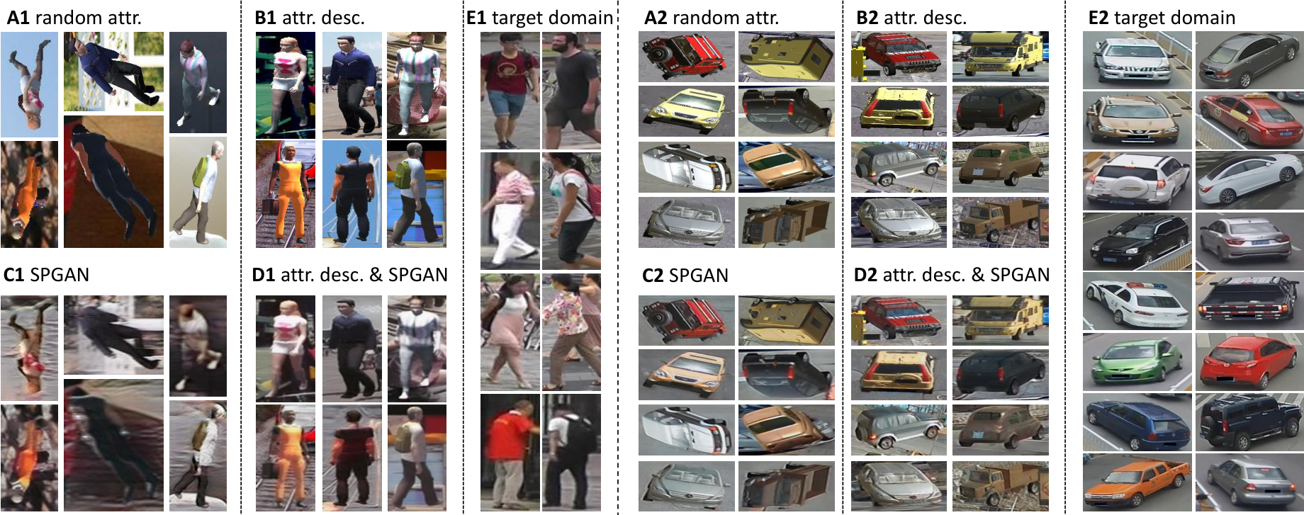
Data synthesis that can be conveniently performed in graphic engines provides invaluable convenience and flexibility for the computer vision community [1, 2, 3, 4, 5]. A large number of training data can be synthesized under different combinations of environmental factors from a small number of 3D object models. Despite this convenience, a large domain gap exists between synthetic data and real-world data, which can substantially decrease accuracy when a model trained on synthetic data is tested with real data [6, 3]. The domain gap problem can be addressed from the appearance level [6] or the content level (Fig. 1). The former often translates image style by using a neural network [7], whereas the latter modifies the image content via manipulating editable attributes directly in graphic engines.
We are motivated by the following considerations. First, collecting large-scale real-world datasets with manual labels is expensive. For example, in a multi-camera system like object re-identification (re-ID), an object must be associated across multiple different cameras to obtain ground truth labels: this process is extremely difficult and laborious because objects usually vary in appearance under different cameras. Privacy and data security concerns further add overheads to this process.
Second, the domain gap between datasets exists not only on the appearance level [7], but also on the content level [6]. Take vehicle re-ID as an example. Images in the VehicleID dataset [8] mainly exhibit car rears and fronts, whereas the VeRi-776 dataset [9] covers more diverse viewpoints. This difference in viewpoints is considered an example of content-level discrepancy between datasets. As a result, models trained on VehicleID [8] have a significant accuracy drop when tested on VeRi-776 [9]. Existing domain adaptation methods on the appearance level can alleviate this problem and improve accuracy, but are essentially incapable of handling the content differences.

Given these considerations, this article proposes an attribute descent algorithm to generate synthetic training data 1) in a large scale and inexpensive manner, 2) with a reduced content domain gap with real-world data. In a nutshell, as shown in Fig. 1 A, the proposed attribute descent algorithm can automatically configure simulator attributes, such as camera viewpoint, lighting direction, and object placement, so that the synthesized data are close to real-world data as measured by the Fréchet Inception Distance (FID) [10]. These optimized attributes are subsequently used for training set generation or augmentation, where style-level image translation can be leveraged to further reduce domain discrepancy. To make the above process happen, we define a controllable simulation environment in the graphic engine with editable object and environment attributes, allowing us to generate large training sets by varying these attributes.
We evaluate the effectiveness of synthetic data generated by attribute descent on object-centric tasks: image classification, person re-ID and vehicle re-ID. In these tasks, an image usually contains a single object of interest which is placed approximately in the image center (through either automatic detection or manual cropping). Specifically, image classification aims to distinguish different classes for an input object of interest, while object re-ID targets at differentiating object (person, vehicle) identities. For each of the tasks, we build a synthetic object-centric filming scenario, which contains an object of interest, a camera and a direct lighting source. Compared with complex-scene applications such as semantic segmentation, object-centric tasks require fewer 3D object assets and have simpler layout relationships between assets, smaller environments and fewer attributes to be controlled. These favorable properties simplify the problem addressed and enable in-depth method analysis. More discussions of the application scope of our method are provided in Section VI.
We identify three scenarios in which data synthesized by attribute descent can be effectively applied: training with adapted synthetic data only, augmenting real training data with synthetic data, and visualizing content-level dataset bias. First, after optimizing synthetic data to approximate target distribution (real world), we directly use synthetic data to train object-centric task models for recognition or re-ID. Second, we add the optimized synthetic data to real-world data to enlarge the training set, which is used for training the task model and improving accuracy. In both applications, we demonstrate that optimized synthetic data are superior to those randomly generated and that the inclusion of the former consistently enhances real-world training data. Furthermore, the two applications suggest the existence of content bias in object-centric datasets, and a third and interesting application is understanding dataset content by using obtained attribute value distributions. For example, we visualize that vehicle orientations on a normal two-way road are usually bi-modal, exhibiting two major angles, whereas those in an intersection are more diverse.
Experimentally we show that attribute descent is superior to using random attributes for training set synthesis, when the training is either with synthetic data only or has both synthetic and real data. Moreover, we compare attribute descent with existing gradient-free optimization techniques, namely Bayesian optimization, reinforcement learning, evolutionary algorithm, and random search. We observe that attribute descent leads to a consistently lower domain gap between the generated training set and target set, consequently yielding the model higher accuracy than the competing methods. Additionally, we report that attribute descent promotes more stable convergence than the competing methods. The above indicates the effectiveness of attribute descent for syn2real content-level domain adaptation.
This article is an extension of our conference publication [11]. Three major differences are presented. First, while only vehicle re-ID is studied in [11], our current system is capable of additionally improving person re-ID and image classification tasks. For these new tasks, we collect/extend new/existing 3D assets in the person and generic object domains and customize them into our pipeline. Second, comprehensive geometric modeling of object-camera placement. This introduces an additional in-plane rotation attribute that allows us to model object orientation more flexibly, particularly for generic objects. Third, by approximating real-world datasets with synthetic counterparts, we show that certain aspects of dataset content in real-world data can be numerically understood and visualized by this synthetic proxy. Interesting experimental observations are presented and discussed.
II Related Work
Realistic appearance generation and domain adaptation. Domain adaptation is often achieved by reducing the domain gaps between distributions. To date, a majority of works in this field has focused on discrepancies in appearance or feature level. For the former, a considerable body of research use the cycle generative adversarial network (CycleGAN) [12] and its variants to reduce the appearance gap [7, 13, 14, 15, 16]. The latter models the dependence between two domains by means of feature-level statistics [17], and many moment matching schemes are studied to learn a shared feature representation [18, 19, 20, 21, 22, 23]. Although these works are shown to be effective in reducing the appearance or feature domain gap, a fundamental problem remains to be solved, i.e., the content difference.
| Task | Dataset | #Models | #Classes (IDs) | Attr. |
| Image cla. | VisDA Source [24] | 1,907 | 12 | ✗ |
| ObjectX | 1,400 | 7 | ✓ | |
| Person re-ID | RandPerson [25] | 8,000 | 8,000 | ✗ |
| UnrealPerson [26] | 3,000 | 3,000 | ✗ | |
| PersonX [5] | 1,266 | 1,266 | ✓ | |
| Vehicle re-ID | PAMTRI [27] | 402 | 402 | ✓ |
| VehicleX | 1,362 | 1,362 | ✓ |
Learning from simulated 3D data. Data simulation is an inexpensive way of increasing a training set scale while providing accurate image labels, flexibility in content generation and high resolution. Learning from simulated data finds it applications in image recognition [24], re-identification [5, 27], semantic segmentation [7, 28, 29], navigation [30] and detection [6, 31]. Existing knowledge or estimation of data distribution is usually required during data synthesis in the graphic engine. Some applications directly take what is presented in existing video games such as GTA5, which have pre-defined scenes and objects [1, 32, 33, 34, 24, 35]. Others manually create their own simulation environments and objects [36, 28, 30, 37, 38], and find it is beneficial to use random attribute within a reasonable range to create random content [4, 39, 40]. However, despite being called “random”, the range of random variables still must be specified manually according to experience. Instead, we aim to learn attribute distributions more automatically or with less human experience.
Automatic 3D content creation. Many works aim to automatically create realistic 3D models [41, 42], focusing on intrinsic properties of 3D models such as backbones, geometry and surface. The studied object models include faces [43], persons [44, 45], vehicles [42] and furniture [41]. Departing from these works that mainly study object synthesis, we aim to use the optimized 3D models for downstream task training.
Content creation for task model training. Several recent studies have attempted to automatically generate 3D content for training task models [6, 46, 29, 3]. They are closest to our work. For example, Kar et al. and Devaranjan et al. simulate traffic for training vehicle detection networks [6, 46]. Xue et al. and Ruiz et al. construct street scenes for semantic segmentation model training [29, 3]. Many of these works use reinforcement learning (RL) based algorithms to optimize attributes [6, 46, 29, 3]. In our article, we find RL less effective in object-centric tasks, in which a relatively small number of attributes needed to be optimized. In this sense, our method is an alternative to existing ones and particularly effective in object-centric tasks (see comparisons in Table VIII).
In object-centric vision tasks, a single object of interest usually appears in an image, because manual cropping or detection is used to place the object approximately in the image center. Specifically, the basic image classification problem aims to distinguish different classes for an input image [47, 48, 49, 50]. Another task that we consider is object re-ID [51, 52, 9], which has many robust systems proposed recently [53, 54, 27, 55]. When experimenting on these object-centric tasks, we adopt existing architectures and loss functions with no bells and whistles.
Dataset bias is a critical reason for compromised model performance [56]. For example, many classification datasets [47, 48, 57] are collected from public user repositories, such as Flickr, which may have content bias in terms of object placement, background, rotation, occlusion, lighting conditions etc. The bias may explain why models exhibit lower accuracy on test sets that have a different content bias from the training set [58]. There are some existing approaches for dataset bias visualization. For example, t-distributed stochastic neighbor embedding (t-SNE) can exhibit feature-level data distributions [59]. In comparison, we aim to visualize bias through attributes, i.e., obtaining attribute distributions numerically and drawing them in graphs.

Similarly, depending on the camera condition, location and environment, existing object re-ID datasets usually have their own distinct characteristics or bias [5]. For example, vehicle images in the VehicleID dataset [8] are either captured from car front or back, whereas the VeRi dataset [9] includes a much wider range of viewpoints. Beyond dataset-dataset differences, large differences also exist between cameras in a single dataset [60]. For example, a camera filming a cross road naturally has more vehicles orientation than a camera on a straight road. In this article, we leverage such characteristics to learn attributes for each camera and simultaneously visualize the attribute distributions.
III Simulation Environment
Overall, we aim to build a simulation environment with editable attributes for building large-scale synthetic datasets that are close to the real world. To achieve this, we collect a large number of 3D objects (Section III-A), build a camera model in the graphic engine, define a set of editable attributes (Section III-B), and acquire synthetic images by varying these attributes (Section III-D).
III-A 3D Asset Acquisition
For object-centric tasks, we use 3D assets from three sources. Their details are provided below as well as in Table I, and sample assets are shown in Fig. 2.
We reformat ObjectX from ShapeNet-V2 [61] to simulate classification data. Similarly to ImageNet [47], ShapeNet organizes 3D shapes according to the WordNet hierarchy [62]. From ShapeNet, we select the classes that are also included in the VisDA target dataset (containing real-world images) [24], which are used as our target data. This amounts to 7 classes and 200 models which are randomly selected for each class. During pre-possessing, models in each class are aligned in the same direction and scaled to a uniform size. Table I shows the statistics of ObjectX, and Fig. 2 visualizes some 3D shapes we collected for categories airplane, bus, skateboard, train, motorcycle, and knife.
We use PersonX to simulate person re-ID data. This asset is introduced by Sun et al. [5] and has 1,266 different manually constructed person models (identities), including 547 females and 719 males. PersonX models are hand-crafted by professional 3D modelers, with a special focus on appearance diversity. To explain, the backbone models of PersonX have various ages, hairstyles, and skin colors. For each backbone model, the clothes are also chosen from a diverse range including T-shirts, skirts, jeans, shorts, pants, slacks, etc. With real-world-like textures, these clothes have good visual authenticity. Furthermore, a person can take various actions (e.g., walking, running) when being filmed. Viewpoint alignment and scaling are performed for 3D objects in PersonX.
VehicleX, introduced in our conference paper [11], is used to simulate data for the vehicle re-ID task. It has a wide range of simulated backbone models and textures and adapts well to the variance of real-world datasets. Specifically, it has 272 backbones which are hand-crafted by professional 3D modelers. The backbones include 11 mainstream vehicle types including sedan, SUV, van, hatchback, MPV, pickup, bus, truck, estate, sportscar and RV. On the basis of these backbones, we obtain 1,362 vehicle identities by adding various colored textures or accessories. A comparison of VehicleX with an existing vehicle re-ID dataset (i.e., PAMIRI [27]) is presented in Table I. VehicleX is three times larger than the synthetic dataset PAMTRI in the number of identities, and, similar to ObjectX and PersonX, can potentially render an unlimited number of images by varying the attributes. In VehicleX, similarly to PersonX, vehicle models are aligned to their frontal views and properly scaled. Note that for object (person and vehicle) re-ID, the testing procedure is retrieval; therefore, synthetic data need not to have the same classes with real-world target data. VehicleX has been used as training data in the AI city challenge in CVPR 2020 and CVPR 202111 1 https://www.aicitychallenge.org/.

III-B Camera Model
To capture 2D images of the 3D objects, we create a camera model, as illustrated in Fig. 3. Let the world coordinate system be O, in which the origin is the center of the 3D object, and the axis points toward a certain direction of each class of objects (e.g., the frontal view of airplanes). The camera coordinate system C is denoted by . To ensure that the target is filmed and to simplify the camera model, we hold a prior that the camera is always facing the 3D object, i.e., towards the center of the world coordinate system (or object center). Thus, we define the axis as pointing away from the center of the object.

We proceed to consider extrinsic and intrinsic parameters that transform the world coordinate system into the camera coordinate system. Extrinsic parameters are determined by the rotation matrix and translation vector . includes object rotation and camera rotation. Object rotation includes the azimuth and elevation, which can be represented by the function of camera height and camera distance . Camera rotation involves only in-plane rotation, because we assume that our camera always faces the object. Thus, the rotation matrix is a function of , , and , and can be written as . The translation vector is determined directly by camera height and camera distance , and thus can be written as . For intrinsic parameters, we use a fixed focus length and image resolution . For example, we set the world coordinate system to a resolution of pixels when capturing vehicle images. Given the above extrinsic parameters and intrinsic parameters, the projection matrix can be written as,
| (1) |
Thus, given focal length and resolution , the camera model has 4 remaining attributes to be configured: azimuth , camera height , camera distance and in-plane rotation . These left 4 attributes determine the diverse object-camera placement, thus allowing us to film a variety of images. This camera model is an improved version from our conference paper [11]. The additionally introduced attribute “in-plane rotation” allows us to more flexibly model objects that do not usually “stand” on the ground plane.
III-C Configurable Attributes
Our system has a total of 6 editable attributes, which are considered to be influential on the training set quality and the subsequent testing accuracy. They include azimuth, camera height, camera distance and in-plane rotation, as mentioned in Section III-B, plus two lighting attributes: light direction and light intensity. Several details regarding these attributes are provided below.
- •
Azimuth represents the horizontal viewpoint of an object and takes a value between and .
- •
In-plane rotation controls camera rotation on the axis. Its value is also between and .
- •
Camera height describes the vertical distance of the camera from the ground, from near (numerical value ) to far (numerical value ).
- •
Camera distance determines the horizontal distance between the camera and the object center. This factor, taking values from low (0) to high (100), strongly affects on the imaging resolution (the resolution of the entire camera view is set to 19201080). Imaging viewpoint is impacted by the joint effects of camera height and distance.
- •
Light direction is part of the environment settings. We assume directional parallel light, and the light direction is modeled from east () to west ().
- •
Light intensity is another a critical attribute influencing task performance by creating reflections and shadows. We manually define a reasonable range for intensity, from dark () to light ().
Note that the pre-defined ranges are broad and involves little human assumption. For example, light intensity ranges from fully light to dark. From the ranges, we aim to find their optimal values for effective training dataset construction. Moreover, these 6 attributes (examples shown in Fig. 4) are found important for the three object-centric tasks. For other tasks such as semantic segmentation and object detection, which involve complex environments and multiple objects, other influential attributes, such as object (relative) locations, are influential. In this article, we try to keep our investigation focused and in depth and leave the more complex applications for future work.
III-D Image Capturing Process
In this section, we describe how to film the 3D objects after varying these editable attributes. To establish controllability, we build a Unity-Python interface by using the Unity ML-Agents toolkit [63], which creates a data transmission path between Unity and Python. Specifically, given a list of parameters from Python, Unity accordingly sets up the camera and environment, then takes the picture and obtains the bounding box precisely according to the object size. The bounding box is then sent back to Python for further processing. Our API allows users to easily obtain rendered images without expert knowledge of Unity. The source code of this API has been released22 2 https://github.com/yorkeyao/VehicleX.
We also consider background and occlusion setups in our system. Specifically, during the attribute distribution optimization process with attribute descent, we render images with black backgrounds and no occlusions. After the optimization is complete, we generate synthetic training data using the optimized attributes while adding random background images and occlusions. For example, when synthesizing vehicle re-ID training data, we add background images from the CityFlow dataset [64], and occluders such as lamp posts, billboards and trash cans. Our preliminary experiments show this strategy increases the diversity of the synthesized training data, consequently enabling robust training of the task model. For example, when using synthetic data only and targeting vehicleID, training on synthetic images with black backgrounds and attribute descent produces 24.12% mAP. The further incorporation of random backgrounds and occlusions yields a notable increase of +11.21% mAP over the training dataset that uses black backgrounds. This strategy allows us to train models that are more robust to various backgrounds and occlusions.
IV Proposed Method
IV-A Attribute Distribution Modeling
We model the distribution of the 6 attributes (Section III-C) using Gaussian Mixture Models (GMM). The primary rationale is that for real-world datasets, these attributes usually follow specific patterns. In the image recognition task, patterns often exist with regard to specific categories. For example, photographs of the category clock are usually taken from the front, not the side or back, where the Gaussian distribution would be helpful. Likewise, in the re-ID task, the camera position is usually fixed, so that the camera height and distance of images captured by a certain camera are generally uni-modal. Moreover, pedestrians and vehicles usually move along predefined trajectories, e.g., footpaths for pedestrians and traffic lanes for vehicles. Because multiple moving directions exist on a single path, the object orientations (i.e., the azimuth) of these re-ID data exhibit multi-modal distributions. Of note, this modeling strategy has also been adopted by Ruiz et al. [65]. In addition, using Gaussians and their mixtures to model the distribution of attributes allows us to conveniently analyze and visualize datasets.

Although a GMM is parameterized by its mean and covariance, our preliminary shows that the change in covariance produces a less prominent supervision signal, i.e., has a weaker effect on task accuracy than the mean. This finding is understandable because the mean parameters encode how the majority of images appear and more directly reflect the dataset distribution gap. Although our method can optimize covariance, doing so would significantly increase the search space without notable accuracy gain. Based on the above considerations, we simplify the covariance matrix into a diagonal matrix whose diagonal elements are pre-defined.
Formally, let represent attributes discussed in Section III-C, where stands for the total number of attributes. is the random variable representing the th attribute. As discussed in Section III-C, we have , where , , , , , and denote azimuth, in-plane rotation, camera height, camera distance, light direction, and light intensity, respectively.
Let represent all the learnable parameters, where is the number of these learnable parameters, and , is a single learnable parameter (i.e., mean, as variance is fixed) of one mixture component. Thus, the can be viewed as a concatenated vector of parameters of all GMMs. Subsequently, we use to denote the overall distribution parameterized by , which consists of GMMs. For example, we define the distribution of in-plane rotation attribute using a GMM consisting of three components. For each component, it has a mean value as a learnable parameter. Formally, they are denoted as , , and . For attributes that empirically have simpler distributions, we use GMM with fewer components. For example, we define the camera distance attribute to follow a single-component Gaussian, which has only one learnable parameter .
Furthermore, to make things easier for optimization, we let represent a collection of search spaces for learnable parameters , where , is the search space of parameter . The dimension of is dependant on the attribute . For example, we have , , and are learnable parameters of attribute (in-plane rotation), and their search spaces , which is a 12-dim vector including angles between and with an increment of . A complete attribute distribution and search space description of all the learnable parameters is provided in Section V-B.
IV-B Optimization
To describe the attribute descent optimization process, we introduce the objective function, detail the proposed attribute descent algorithm and then analyze its convergence property.
Objective function. Given real-world target data, we aim to synthesize a dataset that has a minimal (content) distribution difference with it. Formally, we denote the sets of synthetic images and real images as and , respectively, where the synthetic dataset is simulated following the distribution of vector . We further write as , where is the number of images in . is the underlying rendering function of Unity using attribute vector as input and producing a synthetic image . Each attribute vector is sampled from distribution parameterized by , i.e., . We aim to optimize to minimize the distribution difference measure Fréchet Inception Distance (FID) [10] between and . Correspondingly, our objective function is written as:
| (2) |
where
| (3) |
and
| (4) |
In Eq. 4, and denote the mean and covariance matrix, respectively, of the image descriptors of the synthetic dataset , and and are those of the real-world dataset , respectively. is the dimension of the image descriptors, which are extracted by the InceptionV3 model [66] pre-trained on the ImageNet dataset [47].
The benefit of using FID as the loss function is two-fold. First, it does not require ground truths of the target real-world dataset and instead can be computed using target images only. This obviously saves human labeling efforts. Second, because the FID loss is computed between two sets of images, it is much faster to compute than existing methods using the task loss [67, 6]. The latter requires training the task model (e.g., object detection [68]) with the generated training set and uses the obtained model task performance as loss, which is time-consuming.
It is important to note that the objective function (Eq. 2, Eq. 3 and Eq. 4) is non-differentiable with respect to , primarily because the rendering function (through the 3D engine Unity) is not differentiable. As such, we cannot perform optimization by directly using gradient descent.
Attribute descent algorithm. We are motivated by coordinate descent, a classical optimization method that can work under derivative-free scenarios [69]. To find a local minimum, it selects a coordinate direction to perform a step-by-step search and iterates among coordinate directions. Compared with grid search that considers the entire search space, coordinate descent has significantly reduced search space and thus running time.
Our loss function is parameterized by which encodes the distribution of the configurable attributes. Following coordinate descent, we propose attribute descent (Alg. 1) to iteratively optimize each parameter. Specifically, we view each parameter as a coordinate in coordinate descent. In each iteration, we successively vary the value of a parameter so as to move toward a local minimum of the objective function.
Formally, to iteratively optimize the objective function (Eq. 2) with respect to , we first initialize at epoch :
| (5) |
Then at the th epoch, we get from by iteratively solving the single variable optimization problems. Specifically, at th iteration in epoch , we optimize a single parameter in , to its best value in the search space :
| (6) |
where
| (7) |
In Eq. 6 and Eq. 7, an iteration is defined as the duration for which a single parameter undergoes an optimization process (from Step 7 to Step 14 in Alg. 1). An epoch is defined as the duration for which all parameters undergo one attribute descent round.
In attribute descent, each iteration performs a greedy search for a single parameter while values of the other parameters are fixed. Therefore, each iteration finds the best value for a single parameter, and an epoch gives values for the entire parameter vector . In our experiments, the entire optimization process usually converges in 2 epochs.
Convergence characteristics. Attribute descent has the following properties in regarding model convergence.
Fast conditional updates. The problem configuration allows us to individually optimize parameters quickly. As stated in Section IV, we can update each attribute by using discrete values within a range. For example, the search space for azimuth is between and with a interval. Therefore, only 12 iterations are necessary, thus greatly decreasing the computational time. Note that, using attribute descent for complex tasks such as semantic segmentation would be result in a much slower overall procedure because these tasks have many more attributes to optimize.
Strong stability. Attribute descent can steadily converge because of its “one-at-a-time” optimization characteristics. That is, it gradually and greedily updates each parameter if and only if this update can improve the objective function. Compared with “all-at-once” algorithms like gradient descent which requires expert-level training skills to converge, attribute descent is easier to train and more stable in convergence.
Analysis and visualization of the attribute descent process. In Fig. 5, we present how task performance (re-ID accuracy) and domain discrepancy metric (FID) change during the attribute descent process. We observe that attributes are successively optimized when the FID value decreases and the re-ID accuracy mAP increases. Specifically, from the slope of the curves in Fig. 5 A, when optimizing attributes in the order of “orientation -> lighting -> camera pose”, we observe that after orientation attributes (i.e., in-plane rotation and azimuth) are optimized, a large decrease in FID occurs from 147.85 to 91.14 and a large mAP increase occurs from 12.1% to 21.94%. Subsequently, after lighting attributes are optimized, we have -7.2 FID and +10.7% mAP. The optimization of the camera attributes leads to -4.11 FID and +2.4% mAP. These observations illustrate that all the attributes are useful for improving the training data quality. In addition, in Fig. 5 B, the content of generated images becomes increasingly similar to the target real images through the optimization procedure, thus suggesting the effectiveness of attribute descent.
IV-C Application Scenarios
IV-C1 Training with Synthetic Data Only
Setting. In the first application, we use generated synthetic data to replace real-world data for task model training. Specifically, we perform attribute descent to optimize synthetic data toward target data without labels, train task model on the adapted synthetic data, and then test the models on target test sets.
Obtaining target class or camera labels. As stated in Section IV-A, attribute descent requires known class or camera labels, because we observe different attribute distributions for different categories or cameras; examples are shown in Section V-D.
In mining class or camera labels from the unlabeled target domain, we leverage pseudo labels for classification. Specifically, we use the model trained on synthetic data (i.e., ObjectX) for pseudo label assignment with random attributes. Table II shows that the classification model trained on ObjectX achieves 65.0% average top-1 accuracy on the VisDA test set; therefore, the pseudo labels are relatively reliable. After we obtain the pseudo labels for the target domain, we perform attribute descent for each class by following Alg. 1. Because ObjectX includes 7 classes, we optimize 7 attribute lists for the classification task.
For object re-ID, we simply perform attribute descent against each camera in the target domain, in order to simulate images with similar content to those from each camera. For example, we optimize 6 and 20 attribute lists for the Market and VeRi (both are target domains) training sets which have 6 and 20 cameras, respectively. Note that assuming knowledge of the camera label is a common practice in unsupervised domain adaptive re-ID [71].
IV-C2 Augmenting Target Training Data
Setting. For this application, we use synthetic data to augment real-world training data. Specifically, labels of the target data are provided in both attribute descent and task model training. We combine the adapted synthetic data and real-world data and perform two-stage joint training [72] to obtain task models.For the classification task, when labels of the target training set are given, we optimize attributes for each category directly. Likewise, for the re-ID task, when labels for each camera are given, we optimize attributes for each camera.
Two-stage training [72] is conducted in training data augmentation wherein synthetic and real-world data are both used in training. We mix synthetic data and real-world data in the first stage and finetune with real-world data only in the second stage. In CityFlow, for example, in the first stage, we train on both real and synthetic data, where we classify vehicle images into one of the 1,695 (333 real + 1,362 synthetic) identities. In the second stage, we replace the classification layer with a new classifier fine-tuned on the real dataset (333 classes). When conducting the second stage training, we have a lower learning rate than that in the first stage, with details following [72].
IV-C3 Understanding Dataset Content Numerically
Attribute descent provides a numerical way to understand (and sometimes visualize) the content of datasets. Specifically, given a certain category (or camera), we use attribute descent and synthetic models to build a proxy set, which has similar content distribution. After optimization, we can obtain the values of an attribute of interest for each image, and collectively obtain the value distribution for a dataset. We can then use either statistics or visualization tools to understand a certain aspect of the content of a dataset through the attribute. For example, we can visualize the viewpoint distribution in a 3D sphere (as shown in Section V-D). We can also use histograms to present the distribution of lighting intensity of a dataset.
V Experiment
We evaluate the effectiveness of attribute descent on image classification, person re-ID and vehicle re-ID. In all tasks, given target data (Section V-A), we use attribute descent to synthesize a training set that has similar attribute distributions.
V-A Source and Target Datasets
Image classification. We use ObjectX (described in Section III-A) as the source and the VisDA [24] target set as the target domain. The original VisDA target set has 12 classes of real-world images. Among the 12 classes, we select 7 that are also included in ShapeNet V2 [61] and thus ObjectX. A total of 33,125 images are present in the 7 classes. For each class, the ratio of the number of training images to that of testing images is 1:7 or 1:1.
Person re-ID. We use PersonX as a source, and use two real-world datasets as target: Market-1501 (denoted as Market) [51] and DukeMTMC-reID (denoted as Duke) [52]. Market has 1,501 IDs, 12,936 training images and 19,732 gallery images filmed by 6 cameras. A totoal of 751 out of 1,501 IDs are used for training and the remaining 750 are used for testing. The query set includes 3,368 bounding boxes from 750 identities. Duke contains 1,404 IDs and 36,441 images captured by 8 cameras. There are 16,522 images from 702 identities for training, 2,228 query images from another 702 identities and 17,661 gallery images for testing.
Vehicle re-ID. Apart from the synthetic VehicleX dataset, we use three real-world vehicle re-ID datasets as target domain data. VehicleID [8] contains 222,629 images of 26,328 identities. Half the identities are used for training, and the other half are used for testing. Three test splits exists: “Small”, “Medium” and “Large”, representing the number of vehicles in the test set. Specifically, “Small” has 800 vehicles and 7,332 images, “Medium” has 1,600 vehicles and 12,995 images, and “Large” has 2,400 vehicles and 20,038 images. The VeRi-776 dataset [9] contains 49,357 images of 776 vehicles captured by 20 cameras. The vehicle viewpoints and illumination cover a diverse range. The training set has 37,778 images, corresponding to 576 identities; the test set has 11,579 images of 200 identities. There are 1,678 query images. The train / test sets share the same 20 cameras. We use “VeRi” for short in what follows. CityFlow-reID [64] has more complex environments and has 40 cameras in a diverse environment where 34 of them are used in the training set. The dataset has in total 666 IDs where half are used for training and the rest for testing. We use “CityFlow” for short in the following context.
Evaluation protocol. For image classification, we report the top-1 accuracy averaged over all the categories. For object re-ID, we use mean average precision (mAP) and cumulative match curve (CMC) scores to measure system accuracy, e.g., “Rank-1” and “Rank-5”. “Rank-1” denotes the success rate of finding the true match in the first rank, and “Rank-5” means the success rate of ranking at least one true match within the top 5.
| Application | Training data | Type | Val-test split | Model | plane | bus | car | knife | mcycl | sktbrd | train | per-class |
| Synthetic Training | VisDA Source | S | 1:7 | ResNet-50 | 72.13 | 38.57 | 72.40 | 5.20 | 90.41 | 28.67 | 84.51 | 56.0 |
| OX (Ran. Attr.) | S | 1:7 | ResNet-50 | 77.96 | 48.06 | 62.33 | 40.88 | 92.11 | 57.99 | 75.63 | 65.0 | |
| DAN [19] | 81.54 | 47.40 | 64.98 | 53.33 | 80.16 | 63.36 | 79.38 | 67.2 | ||||
| ADDA [73] | 83.01 | 51.01 | 60.11 | 55.65 | 69.63 | 71.03 | 71.91 | 66.0 | ||||
| SHOT [74] | 88.43 | 64.98 | 67.24 | 66.23 | 85.35 | 78.05 | 75.66 | 72.4 | ||||
| OX (Attr. Desc.) | S | 1:7 | ResNet50 | 83.82 | 68.88 | 62.20 | 64.90 | 86.57 | 38.65 | 92.96 | 71.1 | |
| DAN [19] | 86.93 | 67.68 | 69.02 | 46.50 | 84.50 | 56.39 | 92.66 | 72.0 | ||||
| ADDA [73] | 91.88 | 69.00 | 70.26 | 34.38 | 83.67 | 64.81 | 90.69 | 72.1 | ||||
| SHOT [74] | 93.92 | 78.26 | 75.09 | 42.20 | 91.13 | 78.35 | 88.83 | 78.3 | ||||
| Data Augmentation | VisDA Target | R | 1:7 | ResNet-50 | 96.24 | 85.69 | 91.47 | 94.33 | 92.61 | 90.88 | 90.31 | 91.6 |
| VisDA Target+OX (Ran. Attr.) | R+S | 94.89 | 87.18 | 93.55 | 93.39 | 93.77 | 91.03 | 88.69 | 91.8 | |||
| VisDA Target+OX (Attr. Desc.) | R+S | 96.90 | 89.86 | 94.33 | 95.04 | 94.28 | 92.38 | 92.07 | 93.6 | |||
| VisDA Target | R | 1:1 | ResNet-50 | 98.13 | 89.38 | 95.96 | 96.82 | 95.34 | 95.44 | 93.39 | 94.9 | |
| VisDA Target+OX (Ran. Attr.) | R+S | 96.02 | 86.74 | 94.24 | 93.83 | 93.47 | 90.53 | 89.07 | 92.0 | |||
| VisDA Target+OX (Attr. Desc.) | R+S | 98.08 | 91.56 | 95.90 | 96.24 | 96.00 | 96.00 | 94.48 | 95.5 |
| Appl. | Training data | Type | Model | Rank-1 | Rank-5 | mAP |
| Syn. Training | ImageNet | R | IDE [75] | 6.38 | 14.55 | 1.92 |
| Duke | 42.31 | 61.88 | 18.07 | |||
| MSMT | 41.98 | 61.67 | 20.46 | |||
| PX (Ran. Attr.) | S | IDE [75] | 17.01 | 33.49 | 6.30 | |
| PX (Attr. Desc.) | 34.71 | 51.60 | 15.01 | |||
| Data Aug. | Market | R | IDE [75] | 85.30 | 93.82 | 67.84 |
| PCB [76] | 92.49 | 96.85 | 76.67 | |||
| CBN [77] | 94.35 | 97.91 | 83.63 | |||
| TransReid [78] | 94.72 | 98.47 | 88.03 | |||
| Mar.+PX (Ran. Attr.) | R+S | IDE [75] | 84.62 | 94.30 | 67.56 | |
| Mar.+PX (Attr. Desc.) | IDE [75] | 87.23 | 94.60 | 71.17 | ||
| Mar.+PX (Attr. Desc.) | PCB [76] | 92.58 | 97.24 | 79.99 | ||
| Mar.+PX (Attr. Desc.) | TransReid [78] | 95.24 | 98.57 | 88.76 |
| Appl. | Training data | Type | Model | Rank-1 | Rank-5 | mAP |
| ImageNet | R | IDE [75] | 4.76 | 11.09 | 1.63 | |
| Syn. Training | Market | 32.63 | 47.94 | 17.39 | ||
| MSMT | 46.50 | 64.59 | 28.04 | |||
| PX (Ran. Attr.) | S | IDE [75] | 22.17 | 38.96 | 10.09 | |
| PX (Attr. Desc.) | 30.83 | 47.80 | 15.91 | |||
| Data Aug. | Duke | R | IDE [75] | 78.14 | 88.29 | 58.93 |
| PCB [76] | 82.99 | 90.53 | 67.47 | |||
| CBN [77] | 84.82 | 92.51 | 70.13 | |||
| TransReid [78] | 89.90 | 95.74 | 81.23 | |||
| Duke+PX (Ran. Attr.) | R+S | IDE [75] | 75.99 | 87.70 | 55.77 | |
| Duke+PX (Attr. Desc.) | IDE [75] | 78.28 | 89.27 | 59.10 | ||
| Duke+PX (Attr. Desc.) | PCB [76] | 84.25 | 92.15 | 70.71 | ||
| Duke+PX (Attr. Desc.) | TransReid [78] | 90.41 | 96.03 | 81.43 |
V-B Experimental Details
Attribute descent settings. As discussed in Section IV-A, we model the distribution of the 6 attributes using GMM. Specifically, When using GMM, we set the number of Gaussian components to 3, 6, 1, 1, 1, and 1 for in-plane rotation, azimuth, light intensity, light direction, camera height, and camera distance, respectively. Meanwhile, as mentioned in Section IV-A, only means of the Gaussians are optimized, and initialized from the lowest value in the search space. For each learnable mean value in , the search space is specified in the range defined in Section III-C, and their search steps are 12, 12, 10, 6, 10, and 5 for in-plane rotation, azimuth, light intensity, light direction, camera height, and camera distance, respectively.
The covariance matrices are diagonal matrices with pre-defined diagonal elements. Specifically, the diagonal elements are (10, 10, 10), (20, 20, 20, 20, 20, 20), (0.63), (7.07), (0.4) and (0.6) for in-plane rotation, azimuth, light intensity, light direction, camera height, and camera distance, respectively. In attribute descent, the number of epochs of attribute descent is 2, which usually leads to convergence.
| Training data | Type | Model | Small | Medium | Large | ||||||
| Rank-1 | Rank-5 | mAP | Rank-1 | Rank-5 | mAP | Rank-1 | Rank-5 | mAP | |||
| VID | R | RAM [79] | 75.2 | 91.5 | - | 72.3 | 87.0 | - | 67.7 | 84.5 | - |
| AAVER [53] | 74.69 | 93.82 | - | 68.62 | 89.95 | - | 63.54 | 85.64 | - | ||
| GSTE [80] | 75.9 | 84.2 | 75.4 | 74.8 | 83.6 | 74.3 | 74.0 | 82.7 | 72.4 | ||
| VID | R | IDE [75] | 77.35 | 90.28 | 83.10 | 75.24 | 87.45 | 80.73 | 72.78 | 85.56 | 78.51 |
| VID+VX (Ran. Attr.) | R+S | 80.2 | 93.98 | 85.95 | 76.94 | 90.84 | 82.67 | 73.45 | 88.66 | 80.55 | |
| VID+VX (Attr. Desc.) | R+S | 81.50 | 94.85 | 87.33 | 77.62 | 92.20 | 83.88 | 74.87 | 89.90 | 81.35 |
| Appl. | Training data | Type | Model | Rank-1 | Rank-5 | mAP |
| Syn. Training | ImageNet | R | IDE | 30.57 | 47.85 | 8.19 |
| VehicleID [8] | 59.24 | 71.16 | 20.32 | |||
| Cityflow [64] | 69.96 | 81.35 | 26.71 | |||
| VX (Ran. Attr.) | S | IDE [75] | 43.56 | 61.98 | 18.36 | |
| VX (Attr. Desc.) | 51.25 | 67.70 | 21.29 | |||
| Data Aug. | VeRi | R | IDE [75] | 92.73 | 95.99 | 66.54 |
| VANet [81] | 89.78 | 95.99 | 66.34 | |||
| AAVER [53] | 90.17 | 94.34 | 66.35 | |||
| PCB [76] | 94.04 | 98.21 | 72.04 | |||
| VeRi+PAMTRI [27] | R+S | PAMTRI [27] | 92.86 | 96.97 | 71.88 | |
| VeRi+VX (Ran. Attr.) | IDE [75] | 93.21 | 96.20 | 69.28 | ||
| VeRi+VX (Attr. Desc.) | IDE [75] | 93.44 | 97.26 | 70.62 | ||
| VeRi+VX (Attr. Desc.) | PCB [76] | 94.34 | 97.91 | 74.51 |
| Training data | Type | Model | Rank-1 | Rank-20 | mAP |
| CityFlow | R | BA | 49.62 | 80.04 | 25.61 |
| BS | 49.05 | 78.80 | 25.57 | ||
| IDE (CE+Tri.) | 56.75 | 72.24 | 30.21 | ||
| CityFlow+PAMTRI [27] | R+S | PAMTRI [27] | 59.7 | 80.13 | 33.81 |
| CityFlow+VX (Ran. Attr.) | IDE (CE+Tri.) [75] | 63.59 | 82.60 | 35.96 | |
| CityFlow+VX (Attr. Desc.) | IDE (CE+Tri.) [75] | 64.07 | 83.27 | 37.16 |
Image style transformation. For object re-ID (both person and vehicle), we use SPGAN [14] to transfer the appearance of synthetic data to that of the target domain. For image classification, we do not use style transformation.
Task model configuration. For the classification task, we use ResNet-50 [49] to classify the 7 classes. For person re-ID, we use multiple task models, including ID-discriminative embedding (IDE) [75], the part-based convolution (PCB) [76], and TransReid [78]. Note that when implementing these task models, we use their official implementations with default hyperparameters including learning rate and training epochs. For IDE, we adopt the strategy from [82] which uses ResNet-50 [49] and adds batch normalization and removes ReLU after the final feature layer. For PCB, we use the ResNet-50 backbone and vertically partitions an image into six equal horizontal parts. For vehicle re-ID, we also use IDE and PCB. For IDE, we also use the ResNet-50 backbone. For PCB, we use the ResNet-50 backbone and horizontally divide an image into six parts.
V-C Quantitative Evaluation of Attribute Descent
Given a target set, attribute descent allows us to synthesize a dataset that has a similar distribution on the content (attribute) level. In this section, we demonstrate three application scenarios of the synthesized data in object-centric tasks: training with synthetic data only, real-synthetic data augmentation, and dataset bias visualization. In each application scenario, we compare attribute descent with several existing methods.
Effectiveness of attribute descent for synthetic-data-only training. After generating content-adapted synthetic data with attribute descent (visual examples in Fig. 6), we train the subsequent classification / re-ID models with generated synthetic data only. We mainly compare the optimized synthetic dataset with those generated with random attributes, a commonly used baseline in the community [4, 67]. Here, “random” means that attributes follow the uniform distribution, where their value ranges are the same as the search space of learned attributes. Experimental results on the VisDA target set, Market, Duke, VehicleID, VeRi and CityFlow are shown in Table II, Table III, Table IV, Table VIII, Table VI and Table VII, respectively.
From these results, we observe that when using only synthetic data for training, the data generated from learned attributes achieve much higher task accuracy than those generated from random attributes. For example, when adapting ObjectX to VisDA, attribute descent results in a +6.1% improvement in per-class accuracy over using random attributes. When adapting PersonX to Market, attribute descent yields a +7.69% improvement in Rank-1 accuracy over using random attributes. From VehicleX to VeRi, attribute descent again contributes to a +7.69% improvement in Rank-1 accuracy.
Of note, accuracy under this application scenario is usually lower than that of the state of the art or that produced by in-distribution training sets. This difference is understandable, because synthetic data have a relatively low resemblance with respect to the target data in terms of appearance.
Effectiveness of optimized synthetic data in augmenting the target training data. After optimizing attributes to mimic the target domain, we mix the generated synthetic data with the target training data (with labels) to train the recognition / re-ID models. Apart from the two-stage training strategy (see Section IV-C2), no additional training skills are employed. We again compare attribute descent with random attributes. Experimental results for the three object-centric tasks are summarized across Table II, Table III, Table IV, Table V, Table VI and Table VII. Under this application, we also observe consistent improvement brought by the additional synthetic data. For example, from ObjectX to VisDA, the improvement in learned attributes over random attributes is +1.8% in top-1 recognition accuracy. From PersonX to Market and from VehicleX to VeRi, the improvements in mAP are +2.61% and +1.23%, respectively. The improvements appear numerically smaller than those in the “training with synthetic only” setting, because the latter sits on a relatively low baseline due to its appearance discrepancy between source the target data. To summarize, the superiority of attribute descent over random attributes is also shown in Fig. 7.
In image classification, we evaluate two ratios (i.e., 1:1 and 1:7) of the number of training data to that of test data. Table II indicates that our method brings consistent superiority to training with target data only and augmentation with randomly synthesized data under both ratios. When using a 1:1 ratio, the improvement is smaller in magnitude, a finding that is understandable because using more training data would lead to higher baseline accuracy.
In object re-ID, we also demonstrate the benefit of synthetic data augmentation to a few existing models. For example, in Table III, when using IDE, PCB and TransReid architectures, augmenting the training set with optimized synthetic data is consistently beneficial compared with using real data only. Similar observations are made on the PersonX to Duke setting (Table IV) and the VehicleX to VeRi setting (Table VI).
Comparison with existing gradient-free methods. We compared the proposed attribute descent with random search, evolutionary algorithm (i.e., genetic algorithm), Bayesian optimization, and reinforcement learning (i.e., LTS). These methods have been used as a strong baseline in hyper-parameter search and neural architecture search [83], and only reinforcement learning has been previously used for content-level domain adaptation [3].
Specifically, for the random search, we randomly sample attribute values 200 times and choose the attribute list with the best FID score. For the evolutionary algorithm, we use a generic algorithm with a fitness function equal to FID [84]. For Bayesian optimization, we use the pipeline stated in [85]. For reinforcement learning, we reproduce the LTS structure [3] and replace the task loss with the FID score. When comparing these methods, we use the same distribution definition and initialization as attribute descent. For a fair comparison, we report the best results after 200 iterations of training (i.e., computing the FID score 200 times and taking the lowest FID score). Comparison results are shown in Fig. 8 and Table VIII, from which four observations are made.

son between attribute descent and existing gradient-free methods including Bayesian optimization, evolutionary algorithm and LTS. Gray regions show the error bar for loss curves.
First, under the same task network IDE [75], learned attributes (regardless of which optimization method is used) outperform random attributes in both FID and mAP, demonstrating the benefit of attribute learning for alleviating content difference. Second, random search does not perform well in a limited search time. In fact, it is shown that random search is more effective when many unimportant parameters exist [83]. But in our search space, all the attributes significantly contribute to the distribution differences as shown in Fig. 5 and Fig. 11. Third, the evolutionary algorithm, Bayesian optimization, and LTS appear to fall into an inferior local optimum and thus do not produce a lower FID score than attribute descent. To empirically understand such difference, we find that synthetic data optimized by LTS in mimicking the VehicleID dataset exhibit either the car front or rear, whereas VehicleID actually contains both car front and rear. In comparison, our method can sense both directions as it can iterate the entire search space. Fourth, shown in Fig. 8, compared with existing gradient-free methods, attribute descent has the benefit of stable convergence due to its greedy search nature. Given these benefits, attribute descent presents itself as a straightforward yet effective baseline for syn2real content-level domain adaptation.
Positioning among state-of-the-art systems. This article aims to demonstrate the consistent improvement gained through the use of optimized synthetic data, instead of focusing on achieving a new state of the art. Nevertheless, the system augmented with learned synthetic data has very competitive accuracy. Comparisons with several representative state-of-the-art methods are summarized in Table III, Table IV, Table V, Table VI and Table VII. For example, when Market is jointly trained with personX, our system outperforms TransReID [78] with real data only by +0.52% in Rank-1 accuracy. Similarly, on Duke and VehicleID (small), our system exceeds TransReID [78] and GSTE [80] by +0.51% and +5.6% in Rank-1 accuracy. On the VeRi-776 dataset, the mAP of our system using the PCB backbone is 74.51%, which is +2.63% higher than that using PAMTRI [27].
Impact of attribute order in attribute descent. In Fig. 10, we investigate the dependency among attributes by testing whether the order of attributes matters in attribute descent. Using different attribute orders in attribute descent optimization and comparing the FID scores between generated data and target data at epoch I and epoch II, yields two observations. First, after the first epoch, some orders generate lower FIDs than others. For example, the order “orientation -> lighting -> camera pose” results in lower FID than “lighting -> camera pose -> orientation”. This difference is because orientation accounts more for the discrepancy between synthetic data and real data than camera pose and lighting. Second, although different orders may give different FID values after epoch I, their FID values (and accuracy, not shown in this figure) become similar after epoch II. This property is associated with the coordinate descent algorithm, wherein the order of coordinates in the optimization does not affect final performance.
| Training data | Type | FID | Rank-1 | Rank-5 | mAP |
| VeRi | R | 45.39 | 28.00 | 41.11 | 38.59 |
| Cityflow | 75.36 | 38.23 | 53.70 | 45.57 | |
| VX (Ran. Attr.) | S | 134.75 | 18.76 | 30.11 | 22.00 |
| VX (Ran. Sear.) | 109.94 | 21.84 | 35.29 | 26.35 | |
| VX (Evo. Algo.) | 105.14 | 21.97 | 35.78 | 27.12 | |
| VX (Bay. Opti.) | 99.64 | 22.57 | 38.15 | 30.05 | |
| VX (LTS) | 95.27 | 24.03 | 38.62 | 32.21 | |
| VX (Attr. Desc.) | 77.96 | 28.04 | 41.85 | 35.33 |
Impact of different attributes. We perform ablation studies on each group of attributes: object orientation, camera pose and lighting. Results on the application of training with synthetic data only, and tasks of classification, person re-ID, and vehicle re-ID are summarized in Fig. 11. The results provide us with interesting insights regarding the importance of different attributes in these tasks. First, we observe that all three groups of attributes are necessary for good optimization results, where omitting any of them would decrease the accuracy. For example, when we use random values for orientation attributes, task accuracy drops by 15.7% and 9.95% in top-1 recognition rate and mAP on classification and person re-ID task, respectively. Second, we find that attributes have different importance. Specifically, orientation attributes are the most important. For example, in the vehicle re-ID task, not optimizing vehicle orientation leads to a -10.52% drop in mAP, while is much more than the drop caused by omitting camera pose (-3.54%) and lighting (-1.6%).


V-D Numerically Understanding Dataset Content
This section uses viewpoint as an example to showcase the application of attribute descent in numerically understanding dataset content. As shown in Fig. 9 and Fig. 12, after performing attribute descent on the corresponding synthetic assets, we plot obtained viewpoint value distributions on the unit sphere, where each point on the unit sphere represents a camera pointing toward the center of sphere.The blue points show in-plane rotation of . The orange points indicate in-plane rotation of .
Viewpoint distribution and bias for various classes in VisDA. In Fig. 9 (right) and Fig. 12 A, we observe a significant viewpoint bias in the five categories. For example, we find that airplane, car and bus are usually filmed vertically (in a normal erect position), because the in-plane rotation angles learned for the three class are usually less than 30 degrees. In contrast, knife and skateboard are often filmed from a certain oblique angle with significant in-plane rotations. Moreover, when capturing airplane, bus and skateboard images, the camera is usually at the same height as the object, but for knife, it is usually as either a higher or lower position.
Viewpoint distribution and bias for different cameras in re-ID datasets. In Fig. 12 B-E, we observe very different viewpoint patterns of different cameras. On the Market dataset, the viewpoint distribution for camera 2 is distinct from that for camera 3. Specifically, we observe that camera 2 is higher than camera 3 and the azimuth of camera 2 covers a broader range than that of camera 3. Likewise, on the Duke dataset, camera 4 mainly films people from front or rear angles, whereas camera 7 films from nearly all directions of the azimuth. Similar phenomena are also observed in vehicle re-ID datasets. In VeRi, for example, in contrast to camera 8, which films only car fronts and car rears, camera 7 mainly films vehicles from the side. In summary, significant viewpoint bias exist for different cameras in re-ID datasets. Such bias comes from the fact that camera positions are usually fixed and that objects (person or vehicle) regularly follow predefined lanes. Bias among cameras inevitably leads to bias between datasets, and potentially decrease accuracy when deploying models.
VI Discussion
Optimization under non-differentiable simulation functions. Our system is non-differentiable because of the Unity rendering function. Under this circumstance, the gradient can be estimated by a few existing methods such as finite-difference [6] and reinforcement learning [3]. These methods are best applied in scenarios with a relatively large number of parameters (at least hundreds or thousands) to optimize. However, in object-centric tasks, far fewer attributes to optimize, so we instead propose a stable and efficient optimization approach.
The relationship between distribution shift and task accuracy has been examines in several recent studies. Deng et al. assume a fixed training set and quantitatively measure the strong negative correlation between accuracy and distribution shift of the test set in image classification [86, 87]. In comparison, we assume a fixed test set instead and use the negative correlation in method design: a better training set would have a smaller distribution shift from the test set. This assumption is verified in both object classification and re-ID, which complements [86, 87] from both the assumption and application perspectives.
Can we use metrics other than FID to provide supervision signals? Two other methods could potentially be used to measure distribution gaps: building a discriminator with an adversarial loss or training a task network with the task loss. However, in our preliminary experiment, the discriminator method is prone to detecting the large difference between synthetic and real data and thus continually tells the generator that its generated data have poor quality. This problem breaks the Nash equilibrium between the generator and discriminator, thus hindering us from obtaining an effective generator. On the other hand, a task network can provide accurate supervision signals but is infeasible when target domain labels are not provided. Furthermore, for object re-ID which is evaluated across cameras, the overall supervision provided by the task network does not reflect the training data quality in single cameras and thus poses difficulty in synthesizing data in each camera. As a result, we focus on the difference between features, using FID [10] to quantitatively measure the distribution difference between two datasets.
Application scope. To demonstrate the effectiveness of attribute descent, this article focuses on object-centric tasks, which are either fundamental or have very important applications in the real world, and a relatively small number of attributes are involved. Under these scenarios, attribute descent has quicker convergence and superior performance compared with existing gradient-free optimization methods. As such, the attribute decent serves as an effective baseline for object-centric content-level domain adaptation.
Beyond object-centric tasks, we experimentally show that attribute descent is also useful in the semantic segmentation task where the street scenes have more complex distributions. For this application, we use the 3D assets (i.e., SceneX) collected in our previous work [29], where 23 controllable attributes are defined, including scene layout, illumination, etc. This is significantly more than the 6 attributes defined in the object-centric tasks. Using the Cityscapes dataset [88] as target and DeepLab-v2 segmentation model [89], we present quantitative results in Fig.13. In spite of the more challenging setup, we find that our method still maintains its superiority to random attributes. For example, under synthetic only training, attribute descent yields +6.42% improvement in mean intersection over union (mIoU) over the use of random attributes. That said, inheriting from coordinate descent, attribute descent may have lower running efficiency in a complex scenario [90], where we speculate that global optimization algorithms like reinforcement learning will be good alternatives.
VII Conclusion
This article studies how to improve training data quality from the perspective of reducing the domain gap between synthetic data and real data on the content level. Specifically, we propose an attribute descent algorithm that can automatically edit the source domain (synthetic) image content in a graphic engine to generate training data with a good resemblance to the target domain (real world). We evaluate this method on object-centric tasks, in which the usage of object bounding boxes decreases the number of attributes to be optimized. Fewer attributes of interest allow us to optimize attributes individually using the proposed attribute descent approach. We show that data synthesized from learned attributes improve task accuracy in two application scenarios: training with synthetic data only and augmenting target data with synthetic data. In addition, using viewpoint as an example, we show that attribute descent enables understanding of the dataset content by computing the attribute distribution of given categories or cameras. This article demonstrates the benefit of training data engineering, and in the future, more investigations will be performed to understand training data quality.
Acknowledgement
This work was supported in part by the ARC Discovery Early Career Researcher Award (DE200101283) and the ARC Discovery Project (DP210102801).
References
- [1] S. R. Richter, V. Vineet, S. Roth, and V. Koltun, “Playing for data: Ground truth from computer games,” in European Conference on Computer Vision, 2016.
- [2] C. Sakaridis, D. Dai, and L. Van Gool, “Semantic foggy scene understanding with synthetic data,” International Journal of Computer Vision, pp. 1–20, 2018.
- [3] N. Ruiz, S. Schulter, and M. Chandraker, “Learning to simulate,” in Proceedings of the International Conference on Learning Representations, 2019.
- [4] J. Tremblay, A. Prakash, D. Acuna, M. Brophy, V. Jampani, C. Anil, T. To, E. Cameracci, S. Boochoon, and S. Birchfield, “Training deep networks with synthetic data: Bridging the reality gap by domain randomization,” in Proceedings of the IEEE/CVF Conference on Computer Vision and Pattern Recognition Workshops, 2018.
- [5] X. Sun and L. Zheng, “Dissecting person re-identification from the viewpoint of viewpoint,” in Proceedings of the IEEE/CVF Conference on Computer Vision and Pattern Recognition, 2019.
- [6] A. Kar, A. Prakash, M.-Y. Liu, E. Cameracci, J. Yuan, M. Rusiniak, D. Acuna, A. Torralba, and S. Fidler, “Meta-sim: Learning to generate synthetic datasets,” in Proceedings of the IEEE International Conference on Computer Vision, 2019.
- [7] J. Hoffman, E. Tzeng, T. Park, J.-Y. Zhu, P. Isola, K. Saenko, A. Efros, and T. Darrell, “Cycada: Cycle-consistent adversarial domain adaptation,” in International Conference on Machine Learning, 2018.
- [8] H. Liu, Y. Tian, Y. Yang, L. Pang, and T. Huang, “Deep relative distance learning: Tell the difference between similar vehicles,” in Proceedings of the IEEE/CVF Conference on Computer Vision and Pattern Recognition, 2016.
- [9] X. Liu, W. Liu, H. Ma, and H. Fu, “Large-scale vehicle re-identification in urban surveillance videos,” in The IEEE International Conference on Multimedia and Expo, 2016.
- [10] M. Heusel, H. Ramsauer, T. Unterthiner, B. Nessler, and S. Hochreiter, “Gans trained by a two time-scale update rule converge to a local nash equilibrium,” in Advances in neural information processing systems, 2017.
- [11] Y. Yao, L. Zheng, X. Yang, M. Naphade, and T. Gedeon, “Simulating content consistent vehicle datasets with attribute descent,” in Proceedings of the European Conference on Computer Vision, 2020.
- [12] J.-Y. Zhu, T. Park, P. Isola, and A. A. Efros, “Unpaired image-to-image translation using cycle-consistent adversarial networks,” in Proceedings of the IEEE/CVF Conference on Computer Vision and Pattern Recognition, 2017.
- [13] A. Shrivastava, T. Pfister, O. Tuzel, J. Susskind, W. Wang, and R. Webb, “Learning from simulated and unsupervised images through adversarial training,” in Proceedings of the IEEE/CVF Conference on Computer Vision and Pattern Recognition, 2017.
- [14] W. Deng, L. Zheng, Q. Ye, G. Kang, Y. Yang, and J. Jiao, “Image-image domain adaptation with preserved self-similarity and domain-dissimilarity for person re-identification,” in Proceedings of the IEEE/CVF Conference on Computer Vision and Pattern Recognition, 2018.
- [15] Y. Li, L. Yuan, and N. Vasconcelos, “Bidirectional learning for domain adaptation of semantic segmentation,” in Proceedings of the IEEE/CVF Conference on Computer Vision and Pattern Recognition, 2019, pp. 6936–6945.
- [16] Y.-C. Chen, Y.-Y. Lin, M.-H. Yang, and J.-B. Huang, “Crdoco: Pixel-level domain transfer with cross-domain consistency,” in Proceedings of the IEEE/CVF Conference on Computer Vision and Pattern Recognition, 2019, pp. 1791–1800.
- [17] W. M. Kouw, L. J. Van Der Maaten, J. H. Krijthe, and M. Loog, “Feature-level domain adaptation,” The Journal of Machine Learning Research, vol. 17, no. 1, pp. 5943–5974, 2016.
- [18] B. Sun, J. Feng, and K. Saenko, “Return of frustratingly easy domain adaptation,” in Proceedings of the AAAI Conference on Artificial Intelligence, vol. 30, no. 1, 2016.
- [19] M. Long, Y. Cao, J. Wang, and M. Jordan, “Learning transferable features with deep adaptation networks,” in Proceedings of International Conference on Machine Learning, 2015, pp. 97–105.
- [20] E. Tzeng, J. Hoffman, N. Zhang, K. Saenko, and T. Darrell, “Deep domain confusion: Maximizing for domain invariance,” arXiv preprint arXiv:1412.3474, 2014.
- [21] X. Peng, Q. Bai, X. Xia, Z. Huang, K. Saenko, and B. Wang, “Moment matching for multi-source domain adaptation,” in Proceedings of the IEEE/CVF International Conference on Computer Vision, 2019, pp. 1406–1415.
- [22] Z. Zhang, M. Wang, Y. Huang, and A. Nehorai, “Aligning infinite-dimensional covariance matrices in reproducing kernel hilbert spaces for domain adaptation,” in Proceedings of the IEEE/CVF Conference on Computer Vision and Pattern Recognition, 2018, pp. 3437–3445.
- [23] Y. Zou, X. Yang, Z. Yu, V. Kumar, and J. Kautz, “Joint disentangling and adaptation for cross-domain person re-identification,” in European Conference on Computer Vision, 2020.
- [24] X. Peng, B. Usman, N. Kaushik, J. Hoffman, D. Wang, and K. Saenko, “Visda: The visual domain adaptation challenge,” arXiv preprint arXiv:1710.06924, 2017.
- [25] Y. Wang, S. Liao, and L. Shao, “Surpassing real-world source training data: Random 3d characters for generalizable person re-identification,” in Proceedings of the 28th ACM International Conference on Multimedia, 2020, pp. 3422–3430.
- [26] T. Zhang, L. Xie, L. Wei, Z. Zhuang, Y. Zhang, B. Li, and Q. Tian, “Unrealperson: An adaptive pipeline towards costless person re-identification,” in Proceedings of the IEEE/CVF Conference on Computer Vision and Pattern Recognition, 2021, pp. 11 506–11 515.
- [27] Z. Tang, M. Naphade, S. Birchfield, J. Tremblay, W. Hodge, R. Kumar, S. Wang, and X. Yang, “Pamtri: Pose-aware multi-task learning for vehicle re-identification using highly randomized synthetic data,” in Proceedings of the IEEE International Conference on Computer Vision, 2019.
- [28] A. Gaidon, Q. Wang, Y. Cabon, and E. Vig, “Virtual worlds as proxy for multi-object tracking analysis,” in Proceedings of the IEEE/CVF Conference on Computer Vision and Pattern Recognition, 2016.
- [29] Z. Xue, W. Mao, and L. Zheng, “Learning to simulate complex scenes for street scene segmentation,” IEEE Transactions on Multimedia, 2021.
- [30] E. Kolve, R. Mottaghi, D. Gordon, Y. Zhu, A. Gupta, and A. Farhadi, “Ai2-thor: An interactive 3d environment for visual ai,” arXiv preprint arXiv:1712.05474, 2017.
- [31] Y. Hou, L. Zheng, and S. Gould, “Multiview detection with feature perspective transformation,” in Proceedings of the European Conference on Computer Vision, 2020.
- [32] S. Xiang, Y. Fu, G. You, and T. Liu, “Unsupervised domain adaptation through synthesis for person re-identification,” in Proceedings of the IEEE International Conference on Multimedia and Expo, 2020, pp. 1–6.
- [33] Y.-T. Hu, H.-S. Chen, K. Hui, J.-B. Huang, and A. G. Schwing, “Sail-vos: Semantic amodal instance level video object segmentation-a synthetic dataset and baselines,” in Proceedings of the IEEE/CVF Conference on Computer Vision and Pattern Recognition, 2019.
- [34] Q. Wang, J. Gao, W. Lin, and Y. Yuan, “Learning from synthetic data for crowd counting in the wild,” in Proceedings of the IEEE/CVF Conference on Computer Vision and Pattern Recognition, 2019, pp. 8198–8207.
- [35] A.-D. Doan, A. M. Jawaid, T.-T. Do, and T.-J. Chin, “G2d: from gta to data,” arXiv preprint arXiv:1806.07381, 2018.
- [36] A. Dosovitskiy, G. Ros, F. Codevilla, A. Lopez, and V. Koltun, “Carla: An open urban driving simulator,” arXiv preprint arXiv:1711.03938, 2017.
- [37] M. Deitke, W. Han, A. Herrasti, A. Kembhavi, E. Kolve, R. Mottaghi, J. Salvador, D. Schwenk, E. VanderBilt, M. Wallingford et al., “Robothor: An open simulation-to-real embodied ai platform,” in Proceedings of the IEEE/CVF Conference on Computer Vision and Pattern Recognition, 2020, pp. 3164–3174.
- [38] M. Mueller, V. Casser, J. Lahoud, N. Smith, and B. Ghanem, “Sim4cv: A photo-realistic simulator for computer vision applications,” International Journal of Computer Vision, 08 2017.
- [39] J. Tobin, R. Fong, A. Ray, J. Schneider, W. Zaremba, and P. Abbeel, “Domain randomization for transferring deep neural networks from simulation to the real world,” in 2017 IEEE/RSJ international conference on intelligent robots and systems (IROS). IEEE, 2017, pp. 23–30.
- [40] M. Mozifian, A. Zhang, J. Pineau, and D. Meger, “Intervention design for effective sim2real transfer,” arXiv preprint arXiv:2012.02055, 2020.
- [41] R. K. Jones, T. Barton, X. Xu, K. Wang, E. Jiang, P. Guerrero, N. J. Mitra, and D. Ritchie, “Shapeassembly: Learning to generate programs for 3d shape structure synthesis,” ACM Transactions on Graphics (TOG), vol. 39, no. 6, pp. 1–20, 2020.
- [42] K. Yin, J. Gao, M. Shugrina, S. Khamis, and S. Fidler, “3dstylenet: Creating 3d shapes with geometric and texture style variations,” in Proceedings of the IEEE/CVF International Conference on Computer Vision, 2021, pp. 12 456–12 465.
- [43] T. Shi, Y. Yuan, C. Fan, Z. Zou, Z. Shi, and Y. Liu, “Face-to-parameter translation for game character auto-creation,” in Proceedings of the IEEE/CVF International Conference on Computer Vision, 2019, pp. 161–170.
- [44] Y. Zhang, M. Hassan, H. Neumann, M. J. Black, and S. Tang, “Generating 3d people in scenes without people,” in Proceedings of the IEEE/CVF Conference on Computer Vision and Pattern Recognition, 2020, pp. 6194–6204.
- [45] D. Paschalidou, A. Katharopoulos, A. Geiger, and S. Fidler, “Neural parts: Learning expressive 3d shape abstractions with invertible neural networks,” in Proceedings of the IEEE/CVF Conference on Computer Vision and Pattern Recognition, 2021, pp. 3204–3215.
- [46] J. Devaranjan, A. Kar, and S. Fidler, “Meta-sim2: Unsupervised learning of scene structure for synthetic data generation,” in European Conference on Computer Vision. Springer, 2020, pp. 715–733.
- [47] J. Deng, W. Dong, R. Socher, L.-J. Li, K. Li, and L. Fei-Fei, “Imagenet: A large-scale hierarchical image database,” in Proceedings of the IEEE/CVF Conference on Computer Vision and Pattern Recognition, 2009.
- [48] T.-Y. Lin, M. Maire, S. Belongie, J. Hays, P. Perona, D. Ramanan, P. Dollár, and C. L. Zitnick, “Microsoft coco: Common objects in context,” in European conference on computer vision. Springer, 2014, pp. 740–755.
- [49] K. He, X. Zhang, S. Ren, and J. Sun, “Deep residual learning for image recognition,” in Proceedings of the IEEE/CVF Conference on Computer Vision and Pattern Recognition, 2016, pp. 770–778.
- [50] K. Simonyan and A. Zisserman, “Very deep convolutional networks for large-scale image recognition,” arXiv preprint arXiv:1409.1556, 2014.
- [51] L. Zheng, L. Shen, L. Tian, S. Wang, J. Wang, and Q. Tian, “Scalable person re-identification: A benchmark,” in Proceedings of the IEEE International Conference on Computer Vision, 2015.
- [52] E. Ristani, F. Solera, R. Zou, R. Cucchiara, and C. Tomasi, “Performance measures and a data set for multi-target, multi-camera tracking,” in European Conference on Computer Vision workshop on Benchmarking Multi-Target Tracking, 2016.
- [53] P. Khorramshahi, A. Kumar, N. Peri, S. S. Rambhatla, J.-C. Chen, and R. Chellappa, “A dual path modelwith adaptive attention for vehicle re-identification,” in Proceedings of the IEEE International Conference on Computer Vision, 2019.
- [54] Z. Wang, L. Tang, X. Liu, Z. Yao, S. Yi, J. Shao, J. Yan, S. Wang, H. Li, and X. Wang, “Orientation invariant feature embedding and spatial temporal regularization for vehicle re-identification,” in Proceedings of the IEEE International Conference on Computer Vision, 2017.
- [55] Y. Zhou and L. Shao, “Aware attentive multi-view inference for vehicle re-identification,” in Proceedings of the IEEE/CVF Conference on Computer Vision and Pattern Recognition, 2018.
- [56] A. Torralba and A. A. Efros, “Unbiased look at dataset bias,” in Proceedings of the European Conference on Computer Vision, 2011.
- [57] A. Kuznetsova, H. Rom, N. Alldrin, J. Uijlings, I. Krasin, J. Pont-Tuset, S. Kamali, S. Popov, M. Malloci, A. Kolesnikov et al., “The open images dataset v4,” International Journal of Computer Vision, vol. 128, no. 7, pp. 1956–1981, 2020.
- [58] A. Barbu, D. Mayo, J. Alverio, W. Luo, C. Wang, D. Gutfreund, J. Tenenbaum, and B. Katz, “Objectnet: A large-scale bias-controlled dataset for pushing the limits of object recognition models,” in Advances in Neural Information Processing Systems, 2019.
- [59] L. Van der Maaten and G. Hinton, “Visualizing data using t-sne.” Journal of machine learning research, vol. 9, no. 11, 2008.
- [60] Z. Zhong, L. Zheng, Z. Zheng, S. Li, and Y. Yang, “Camstyle: A novel data augmentation method for person re-identification,” IEEE Transactions on Image Processing, vol. 28, no. 3, pp. 1176–1190, 2018.
- [61] A. X. Chang, T. Funkhouser, L. Guibas, P. Hanrahan, Q. Huang, Z. Li, S. Savarese, M. Savva, S. Song, H. Su et al., “Shapenet: An information-rich 3d model repository,” arXiv preprint arXiv:1512.03012, 2015.
- [62] G. A. Miller, “Wordnet: a lexical database for english,” Communications of the ACM, vol. 38, no. 11, pp. 39–41, 1995.
- [63] A. Juliani, V.-P. Berges, E. Vckay, Y. Gao, H. Henry, M. Mattar, and D. Lange, “Unity: A general platform for intelligent agents,” arXiv preprint arXiv:1809.02627, 2018.
- [64] Z. Tang, M. Naphade, M.-Y. Liu, X. Yang, S. Birchfield, S. Wang, R. Kumar, D. Anastasiu, and J.-N. Hwang, “Cityflow: A city-scale benchmark for multi-target multi-camera vehicle tracking and re-identification,” in Proceedings of the IEEE/CVF Conference on Computer Vision and Pattern Recognition, 2019.
- [65] N. Ruiz, S. Schulter, and M. Chandraker, “Learning to simulate,” in Proceedings of the International Conference on Learning Representations, 2018.
- [66] C. Szegedy, V. Vanhoucke, S. Ioffe, J. Shlens, and Z. Wojna, “Rethinking the inception architecture for computer vision,” in Proceedings of the IEEE/CVF Conference on Computer Vision and Pattern Recognition, 2016.
- [67] T. Kim, M. Cha, H. Kim, J. K. Lee, and J. Kim, “Learning to discover cross-domain relations with generative adversarial networks,” in International Conference on Machine Learning, 2017.
- [68] R. Girshick, “Fast r-cnn,” in Proceedings of the IEEE international conference on computer vision, 2015, pp. 1440–1448.
- [69] S. J. Wright, “Coordinate descent algorithms,” Mathematical Programming, vol. 151, no. 1, pp. 3–34, 2015.
- [70] W. Deng, L. Zheng, Q. Ye, Y. Yang, and J. Jiao, “Similarity-preserving image-image domain adaptation for person re-identification,” arXiv preprint arXiv:1811.10551, 2018.
- [71] Z. Zhong, L. Zheng, Z. Zheng, S. Li, and Y. Yang, “Camstyle: A novel data augmentation method for person re-identification,” IEEE Transactions on Image Processing, vol. 28, no. 3, pp. 1176–1190, 2019.
- [72] Z. Zheng, T. Ruan, Y. Wei, and Y. Yang, “Vehiclenet: Learning robust feature representation for vehicle re-identification,” in Proceedings of the IEEE/CVF Conference on Computer Vision and Pattern Recognition Workshops, 2019.
- [73] E. Tzeng, J. Hoffman, K. Saenko, and T. Darrell, “Adversarial discriminative domain adaptation,” in Proceedings of the IEEE International Conference on Computer Vision, 2017.
- [74] J. Liang, D. Hu, and J. Feng, “Do we really need to access the source data? source hypothesis transfer for unsupervised domain adaptation,” in International Conference on Machine Learning. PMLR, 2020, pp. 6028–6039.
- [75] L. Zheng, Z. Bie, Y. Sun, J. Wang, C. Su, S. Wang, and Q. Tian, “Mars: A video benchmark for large-scale person re-identification,” in European Conference on Computer Vision, 2016.
- [76] Y. Sun, L. Zheng, Y. Yang, Q. Tian, and S. Wang, “Beyond part models: Person retrieval with refined part pooling (and a strong convolutional baseline),” in European Conference on Computer Vision, 2018.
- [77] Z. Zhuang, L. Wei, L. Xie, T. Zhang, H. Zhang, H. Wu, H. Ai, and Q. Tian, “Rethinking the distribution gap of person re-identification with camera-based batch normalization,” in European Conference on Computer Vision. Springer, 2020, pp. 140–157.
- [78] S. He, H. Luo, P. Wang, F. Wang, H. Li, and W. Jiang, “Transreid: Transformer-based object re-identification,” in Proceedings of the IEEE International Conference on Computer Vision, 2021.
- [79] X. Liu, S. Zhang, Q. Huang, and W. Gao, “Ram: a region-aware deep model for vehicle re-identification,” in The IEEE International Conference on Multimedia and Expo, 2018.
- [80] Y. Bai, Y. Lou, F. Gao, S. Wang, Y. Wu, and L.-Y. Duan, “Group-sensitive triplet embedding for vehicle reidentification,” IEEE Transactions on Multimedia, vol. 20, no. 9, pp. 2385–2399, 2018.
- [81] R. Chu, Y. Sun, Y. Li, Z. Liu, C. Zhang, and Y. Wei, “Vehicle re-identification with viewpoint-aware metric learning,” in Proceedings of the IEEE International Conference on Computer Vision, 2019.
- [82] H. Luo, Y. Gu, X. Liao, S. Lai, and W. Jiang, “Bag of tricks and a strong baseline for deep person re-identification,” in Proceedings of the IEEE/CVF Conference on Computer Vision and Pattern Recognition Workshops, 2019.
- [83] J. Bergstra and Y. Bengio, “Random search for hyper-parameter optimization,” Journal of machine learning research, vol. 13, no. Feb, pp. 281–305, 2012.
- [84] L. Xie and A. Yuille, “Genetic cnn,” in Proceedings of the IEEE international conference on computer vision, 2017, pp. 1379–1388.
- [85] B. Shahriari, K. Swersky, Z. Wang, R. P. Adams, and N. De Freitas, “Taking the human out of the loop: A review of bayesian optimization,” Proceedings of the IEEE, vol. 104, no. 1, pp. 148–175, 2015.
- [86] W. Deng and L. Zheng, “Are labels always necessary for classifier accuracy evaluation?” in Proceedings of the IEEE/CVF Conference on Computer Vision and Pattern Recognition, 2021, pp. 15 069–15 078.
- [87] W. Deng, S. Gould, and L. Zheng, “What does rotation prediction tell us about classifier accuracy under varying testing environments?” in International Conference on Machine Learning, 2021.
- [88] M. Cordts, M. Omran, S. Ramos, T. Rehfeld, M. Enzweiler, R. Benenson, U. Franke, S. Roth, and B. Schiele, “The cityscapes dataset for semantic urban scene understanding,” in Proceedings of the IEEE Computer Vision and Pattern Recognition, 2016, pp. 3213–3223.
- [89] L.-C. Chen, G. Papandreou, I. Kokkinos, K. Murphy, and A. L. Yuille, “Deeplab: Semantic image segmentation with deep convolutional nets, atrous convolution, and fully connected crfs,” IEEE Transactions on Pattern Analysis and Machine Intelligence, 2018.
- [90] Y. Nesterov, “Efficiency of coordinate descent methods on huge-scale optimization problems,” SIAM Journal on Optimization, vol. 22, no. 2, pp. 341–362, 2012.
![[Uncaptioned image]](2202.14034v2/Yue.jpg) |
Yue Yao is a Research Officer at the School of Computing, Australian National University. Before that, he studied as a Ph.D. student at the Australian National University. He completed the degree of Bachelor of Advanced Computing at the Australian National University in 2018. His research interests include training set optimization, data synthesis and brain-computer interface. |
![[Uncaptioned image]](2202.14034v2/Liang.jpg) |
Liang Zheng is an Associate Professor at the School of Computing, Australian National University. He received the Ph.D. degree in Electronic Engineering from Tsinghua University, China, in 2015, and the B.E. degree in Life Science from Tsinghua University, China, in 2010. He was a postdoc researcher at the Center for Artificial Intelligence, University of Technology Sydney, Australia (2016 - 2018). His research interests include object re-identification, domain adaptation, deep learning and data synthesis. |
![[Uncaptioned image]](2202.14034v2/Xiaodong-Yang.png) |
Xiaodong Yang is the Head of Machine Learning at QCraft. Previously, he was a Senior Research Scientist at NVIDIA Research. He received the B.S. degree from Huazhong University of Science and Technology, China, in 2009, and the Ph.D. degree from City University of New York, USA, in 2015. His research interests include autonomous driving, image and video understanding, activity and gesture recognition, facial analytics, object re-identification, deep generative modeling, etc. |
![[Uncaptioned image]](2202.14034v2/milind.png) |
Milind Napthade is the Senior Vice President in Capital One. Previously he led the technology and innovation strategy and engineering execution for NVIDIA’s Metropolis platform. He previously served as the program director in the Smarter City Services Group at the IBM T.J. Watson Research Center in Hawthorne, New York, and leader of the Smarter Sustainable Dubuque living lab. Naphade received a Ph.D. in electrical engineering from the University of Illinois at Urbana-Champaign. |
![[Uncaptioned image]](2202.14034v2/TomGedeon-st-rect.jpg) |
Tom Gedeon is the Human-Centric Advancements Chair in AI and Head of the Human-Centric Advancements group in Artificial Intelligence at Curtin University. He is an international Research Professor at Obuda University in Hungary. He is an Honorary Professor at the Australian National University, where he was formerly Deputy Dean and Head of Computer Science. His B.Sc and Ph.D. are from the University of Western Australia, and Grad Dip Management from UNSW. He is twice a former President of the Asia-Pacific Neural Network Assembly, and former President of the Computing Research and Education Association of Australasia. He is an associate editor of the IEEE Transactions on Fuzzy Systems, and the INNS/Elsevier journal Neural Networks. His research interests are in responsive AI and responsible AI. |