Data-driven simulation of Fisher-Kolmogorov tumor growth models using Dynamic Mode Decomposition

The Fisher-Kolmogorov model consists of a second-order reaction-diffusion PDE that describes the propagation of wavefronts in a nonlinear system (see Eq. (1) below). This model has been applied in a myriad of different settings, including population dynamics [45, 44, 5, 16, 20], epidemiology [31, 10], and propagation of domain walls in liquid crystals [22], among others. In the present work, we are most interested in its application to the modeling of untreated solid tumor growth [44, 38, 36, 28, 25, 42, 55, 54]. In this context, the Fisher-Kolmogorov equation describes the spatiotemporal dynamics of the tumor cell density $\phi(\boldsymbol{x},t)$ (cells/mm³) as a combination of two driving mechanisms: the tumor cell mobility, which is represented by the diffusion operator, and the tumor cell net proliferation, which is modeled via the nonlinear logistic reaction term. Denoting the spatial domain by $\Omega\in\mathbb{R}^{n_{d}}$, $n_{d}=1,\,2,\,3$ and the time horizon by $T$, the usual formulation of the model reads as

	$\displaystyle\frac{\partial\phi}{\partial t}$	$\displaystyle=\nabla\cdot\left(D\nabla\phi\right)+\rho\phi\left(1-\frac{\phi}{\theta}\right)\qquad$	$\displaystyle\text{ in }\Omega\times[0,\,T],$		(1)
	$\displaystyle\nabla\phi\cdot\boldsymbol{n}$	$\displaystyle=0\qquad$	$\displaystyle\text{ on }\partial\Omega\times[0,\,T],$		(2)
	$\displaystyle\phi(0,\boldsymbol{x})$	$\displaystyle=\phi_{0}(\boldsymbol{x})\qquad$	$\displaystyle\text{ at }t=0.$		(3)

In Eq. (1), $D$ denotes the diffusion coefficient (mm${}^{n_{d}}$/days), $\rho$ represents the net tumor cell proliferation rate (days^-1), and $\theta$ is the tissue carrying capacity (i.e., the maximum admissible tumor cell density). In general, these parameters may be defined pointwise and over time (i.e., $D=D(\boldsymbol{x},t)$, $\rho=\rho(\boldsymbol{x},t)$, and $\theta=\theta(\boldsymbol{x},t)$), for example, to account for preferential directions of growth, mechanical inhibition of tumor cell mobility and proliferation, the existence of a vascular network supporting tumor development, as well as the local and transient effect of therapies on the mechanisms in the model [44, 38, 36, 28, 25, 42, 55, 54]. However, we will adopt constant values for $D$, $\rho$, and $\theta$ for the sake of simplicity in this initial study on DMD reconstruction of the Fisher-Kolmogorov solutions for tumor forecasting applications. Additionally, we will henceforth set $\theta=1$ in Eq. (1), which is equivalent to assume that $\phi(\boldsymbol{x},t)$ represents the normalized tumor cell density (i.e., such that $0\leq\phi(\boldsymbol{x},t)\leq 1$). Finally, Eq. (2) introduces no-flux boundary conditions, assuming that the tumor grows confined within the considered tissue or organ domain defined by $\Omega$ ($\boldsymbol{n}$ is the outward unit vector normal to $\partial\Omega$) , while Eq. (3) defines the initial conditions.

Eq. (1)-(3) constitute the strong form of the organ-confined untreated solid tumor growth problem. By choosing a test function $v$ in a suitable function space $\mathcal{V}$, we obtain the variational form of (1)-(3) as follows: Find $\phi\in\mathcal{V}$ such that, for all $v\in\mathcal{V}$,

$\displaystyle\int_{\Omega}\frac{\partial\phi}{\partial t}v\,d\Omega+\int_{\Omega}D\nabla\phi\cdot\nabla v\,d\Omega-\int_{\Omega}\rho\phi\left(1-\frac{\phi}{\theta}\right)v\,d\Omega$

$\displaystyle=0,$

(4)

where the Neumann boundary condition (2) makes the boundary integral term arising from the integration-by-parts to vanish. The variational problem (4) is known to admit a unique solution $\phi$, which tends to either the trivial steady state of 0 or a non-trivial, non-negative steady state as $t\to\infty$ [23, 4]. Furthermore, provided $0\leq\phi_{0}\leq 1$, then $0\leq\phi\leq 1$ for all $t$ [4].

DMD is an equation-free data-driven method that extracts the most dynamically relevant structures on data containing spatial and temporal structures based on little to no assumptions on data. These structures are often described as DMD modes and are associated with frequency, and amplification/damping terms [33]. It is known that the considered dataset, even if containing data from nonlinear phenomena, can be reconstructed from a significant smaller portion of DMD modes without compromising accuracy. For instance, a turbulent and highly nonlinear flow containing thousands of DMD modes can be properly reconstructed using only the first one hundred DMD modes [8]. Besides of efficiently reconstructing accurate solutions with a significantly smaller quantity of information, DMD has been applied on a wide range of applications, from model order reduction [3], to control [18], temporal inference [8], and modal analysis [50]. Despite of several variations for specific applications, herein we make use of standard DMD, which we briefly describe below.

For this study, we consider the dataset generated by the numerical simulation of the Fisher-Kolmogorov model described on Section 2.3. Each snapshot $\mathbf{x}_{i}$ - the solution vector obtained each time step $i$ from the numerical simulation - is stacked vertically on a matrix of dimensions $n\times(m+1)$, where $n$ is the number of degrees of freedom of the problem and $m+1$ is the number of time steps for which the solution is computed. This matrix, $\mathbf{X}$, is called Snapshot Matrix. The next step is to split $\mathbf{X}$ into $\mathbf{X}_{1}$ and $\mathbf{X}_{2}$ such that $\mathbf{X}_{1}=[\mathbf{x}_{0}\dotsc\mathbf{x}_{m}]\in\mathbb{R}^{n\times m}$ and $\mathbf{X}_{2}=[\mathbf{x}_{1}\dotsc\mathbf{x}_{m+1}]\in\mathbb{R}^{n\times m}$. The two matrices can be linearly mapped as

$$\mathbf{X}_{2}=\mathbf{A}\mathbf{X}_{1},$$

(5)

where $\mathbf{A}$ maps the dynamics of the evolution in time of the data. Although not being computationally efficient, the computation of $\mathbf{A}$ could be done directly by multiplying $\mathbf{X}_{2}$ to the Moore-Penrose pseudoinverse of $\mathbf{X}_{1}$. This approach is described as the exact DMD and can be formulated as the optimization problem

$$\mathbf{A}=\argmin_{\mathbf{A}}||\mathbf{X}_{2}-\mathbf{A}\mathbf{X}_{1}||_{F}$$

(6)

where $||\cdot||$ is the Frobenius norm. Instead, the pseudoinverse can be approximated by applying the Singular Value Decomposition (SVD) factorization into $\mathbf{X}_{1}$ and preserving the first $r$ singular values and vectors, where $r$ must be carefully chosen to preserve the structures of the matrix. That is:

$$\mathbf{X}_{1}=\mathbf{U}\mathbf{\Sigma}\mathbf{V}^{T},$$

(7)

where $\mathbf{\Sigma}$ are the singular values and $\mathbf{U}$ and $\mathbf{V}$ are the left and right singular vectors, respectively. This approach dramatically reduces the algorithmic complexity of this operation while improving the conditioning of the resulting matrix. However, due to this approximation, the computation of $\mathbf{A}$ is replaced by the computation of $\mathbf{\tilde{A}}$, which is a $r\times r$ projection of $\mathbf{A}$. From this point, the dynamics of the system can be interpreted from the eigenvectors and eigenvalues of $\mathbf{\tilde{A}}$. The DMD modes can be obtained as:

$$\mathbf{\Psi}=\mathbf{X}_{2}\mathbf{V}_{r}\mathbf{\Sigma}^{-1}_{r}\mathbf{W},$$

(8)

where $\mathbf{W}$ are the eigenvectors of $\mathbf{\tilde{A}}$ and the subscript $r$ indicates that $\mathbf{V}$ has been truncated to the first $r$ vectors. Then, the solution of the Fisher-Kolmogorov equation can be reconstructed and extrapolated as:

$$\mathbf{x}(t)\approx\tilde{\mathbf{x}}(t)=\mathbf{\Psi}\exp(\mathbf{\Omega}_{eig}t)\mathbf{b},$$

(9)

with $\mathbf{b}$ being the vector containing the projected initial conditions such that $\mathbf{b}=\mathbf{\Psi^{\dagger}}\mathbf{x}_{0}$, and $\mathbf{\Omega}_{eig}$ is a diagonal matrix whose entries are the continuous eigenvalues $\omega_{i}=\ln(\lambda_{i})/\Delta t_{o}$, where $\Delta t_{o}$ is the time step size between the DMD snapshots.

In this work, we perform a computational study to analyze the numerical performance of our DMD implementation in 2D and 3D test scenarios leveraging clinically-relevant parameter values from the literature [54, 40, 39, 36, 27, 15]. The objectives of the 2D simulation study are to evaluate the ability of DMD to learn and reproduce the dynamics of the Fisher-Kolmogorov tumor growth model, to investigate the potential relationship between the quality of the DMD reconstruction and the model parameters (i.e., $D$ and $\rho$), and to determine whether DMD shows an acceptable performance for any parameter choice or a subregion of the parameter space (i.e., a subset of tumor types). Then, we proceed to assess whether 3D DMD reconstructions obtained for parameter values in this subregion also exhibit a satisfactory performance, which would ultimately support the use of our approach in patient-specific, organ-scale scenarios.

In 2D, we consider an elliptical tumor with diameter lengths of 3 and 5 millimeters that is centered in a square tissue domain of 50$\times$50 millimeters, as shown in Fig. 1. Similarly, in 3D, we study an ellipsoidal tumor with diameter lengths of 5, 3, and 3 millimeters that is centered in a cubic tissue domain of 20$\times$20$\times$20 millimeters (Figure 2). We construct these initial conditions using a hyperbolic tangent hill function that yields $\phi=0.5$ inside the tumor and $\phi=0$ outside:

$$\phi(\boldsymbol{x},0)=\frac{1}{4}-\frac{1}{4}\tanh\left(\frac{100}{\sqrt{2}}\left(\sqrt{\sum_{i=1}^{n_{d}}\frac{\left(x_{i}-c_{i}\right)^{2}}{d_{i}^{2}}}-1\right)\right),$$

(10)

where $\boldsymbol{x}=\{x_{i}\}_{i=1}^{n_{d}}$ is the position vector, $\mathbf{c}=\{c_{i}\}_{i=1}^{n_{d}}$ denotes the center of the domain, and $\{d_{i}\}_{i=1}^{n_{d}}$ are the principal diameters of the tumor initial geometry in $\mathbb{R}^{n_{d}}$.

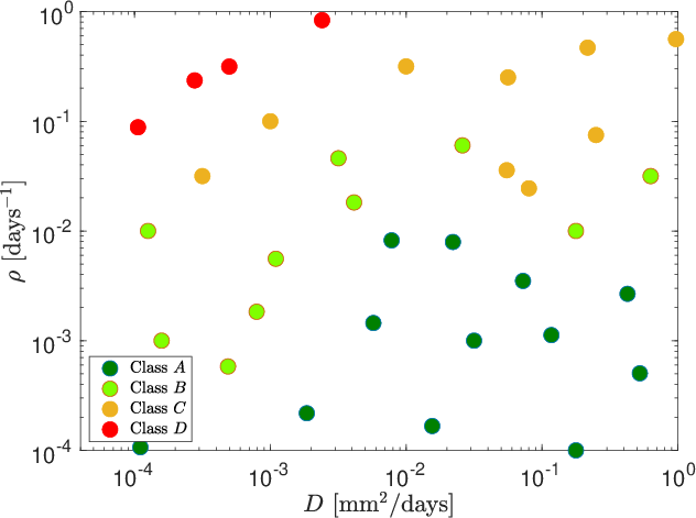
We construct the parameter space by leveraging values of $D$ from 10^-4 to 1 mm²/days and values of $\rho$ from 10^-4 to 1 days^-1. This broad parameter ranges include a wide array of clinically-relevant scenarios as reported in previous computational oncology studies [54, 36, 27]. To explore the performance of our DMD implementation over this parameter space, we sparsely and randomly sample 35 parameter value pairs $\{D,\rho\}$ using Latin hypercube sampling, as shown in Fig. 1 (for numerical data, see Appendix). For the 3D simulation, we let $D=0.00186$ mm³/days, and $\rho=0.00022$ days^-1, which correspond to those used in case 23 in the 2D study. We note that the units of $D$ are now changed to reflect the shift to three spatial dimensions.

The reference simulations of the model are carried out using the libMesh finite element library [32]. In 2D, we discretize the computational domain using 125,000 linear triangular elements. In 3D, we use an adaptive mesh refinement/coarsening scheme (AMR/C). The mesh has initially $10\times 10\times 10$ cells, with each cell divided into 6 linear tetrahedra. We refine the initial region where the tumor is located into four levels and, after the refinement, the smallest element has a size of 0.125 mm. The adaptive mesh refinement is based on the flux jump of the of tumor cell density function error, in which the maximum level of refinement is equal to four. We apply the AMR/C every 20 time steps. Details about the AMR/C procedure may be found in [49, 21]. We output the projected solution to a fixed grid to enable the use of DMD [8]. The projected mesh comprises 288,597 linear tetrahedra elements, with an element size of 0.25 mm. We integrate in time using the second order backward differentiation formula (BDF2) scheme with a constant time step of 0.25 days [27, 28]. The resulting linear systems are solved utilizing the GMRES algorithm with a ILU(0) preconditioner. For both the 2D and the 3D case, we output the solution every 4 time steps.

The DMD method is implemented by leveraging the PADMe¹¹ 1 https://github.com/gf-barros/padme library [9]. We consider 20 modes in our DMD reconstructions, since we empirically observed that they are typically enough to yield sufficient reconstruction capability after preliminary sensitivity analyses of the SVD (see, e.g., [8]). Ideally, we would like DMD computations to provide reasonable approximations for long-term model predictions with minimal-to-moderate training. In such a case, DMD would enable the rapid evaluation of different tumor growth scenarios by requiring the resolution of only a relatively small number of time steps. Thus, in order to evaluate the efficacy of DMD, we compare the performance achieved when leveraging training periods of 20, 50, 100, and 200 days within a fixed time horizon of 365 days. To this end, we evaluate the relative error in $L^{2}$ norm $e_{DMD}^{n}(t)$ at a given instance $t$ as:

$\displaystyle e_{DMD}^{n}(t)$

$\displaystyle=\sqrt{\frac{\displaystyle\int_{\Omega}(\phi_{r}(t)-\phi_{DMD}^{n}(t))^{2}d\Omega}{\displaystyle\int_{\Omega}\phi_{r}(t)^{2}d\Omega}}.$

(11)

where $\phi_{r}$ denotes the value of $\phi$ computed in the reference simulation and $\phi_{DMD}^{n}$ represents the corresponding DMD reconstruction over $n$ training days. We further construct a grading system to characterize the performance of DMD based on $e_{DMD}^{n}(t)$ over the whole time domain and at specific timepoints representing short-to-long-term predictions:

• •

  Class $A$: If a case is such that

  $$\frac{1}{365}\int_{0}^{365}e_{DMD}^{50}(t)dt<0.1,\,\,\text{ and }e_{DMD}^{50}(365)<0.2,$$

  implying that a short training period provides an accurate reconstruction over the whole time interval.

• •

  Class $B$: Cases not in Class $A$ such that:

  $$e_{DMD}^{50}(100)<0.1,\,\,e_{DMD}^{100}(150)<0.1,\,\,e_{DMD}^{200}(250)<0.1,$$

  signifying cases that do not necessarily have good long-term error performance, but are accurate over the medium-to-short term.

• •

  Class $C$: Cases not in Class $A$ or $B$ such that:

  $$e_{DMD}^{200}(250)<1,$$

  meaning cases for which the DMD reconstruction is not necessarily accurate but for which the error remains bounded.

• •

  Class $D$: All other cases, i.e., instances in which DMD does not produce helpful long- or short-term extrapolations, and for which the error may blow up.

We acknowledge that, like all scoring/classification systems, our grading system is to some extent arbitrary. However, we feel that our rigorous criteria provide a reasonable indicators for the qualitative error behaviors which we seek to identify.

Of our 35 cases, we obtained numerical results for 34, with the reference solution of one of the cases (case 17) failing to converge. This case has been classified as a D. In Fig. 3, we show the error performance of one case from each class: case 31 (A), case 11 (B), case 9 (C) and case 13 (D). These give an illustration of the general performance behavior that the classes are designed to indicate. Complete plots of all 34 converged cases cases are shown in Fig. A1-A12. Note these figures have been placed at the end of the manuscript for reasons of readability. We note that the vertical lines mark the end of each training period for the correspondingly-colored DMD reconstruction. We immediately note that DMD works very well for some cases, across all training levels and time intervals, and less well for others.

Applying our grading system to the results, we visualize the classes according to $\rho$ and $D$ in Fig. 4. We see a clear and definite pattern to the results, and the classes form clusters in the parameter space. For moderate to high values of $D$ coupled with low to moderate values of $\rho$, we expect DMD to perform best. In such cases (Class $A$), the long-term accuracy of DMD remains high, even for short training periods. For cases in which the values of $\rho$ and $D$ are both low, we see a deterioration of the long-term error behavior, while the short-term error behavior remains nonetheless strong (Class $B$). Cases in which both $\rho$ and $D$ are high tended to yield less accurate results, while, in cases in which $\rho$ was high but $D$ was low, the DMD reconstructions tend to fail.

We then examined the influence of the maximum real part of the DMD eigenvalues for each case. Given the expression (9), one observes that, if some $\lambda_{i}$ have large real parts, we can expect the DMD performance to deteriorate, particularly for larger $t$. In Fig. 5, we plot max $\text{Re}(\lambda)$ for each case, and analyze its relationship with the ratio $D/\rho$ (left), $D$ (center), and $\rho$ (right). The first thing we note is that max Re($\lambda$) is, as expected, a reliable predictor of the overall DMD performance. The higher-class cases are lower on the vertical axis representing max $\text{Re}(\lambda)$, with lower-class cases towards the higher end. In terms of relationship with the problem parameters, we see moderately strong relationships between Re($\lambda)$ and $D/\rho$, $\rho$, with the relationship less strong between Re($\lambda)$ and $D$. Quantitatively, the log-correlation coefficients are 0.574 between Re($\lambda$) and $D/\rho$, -0.208 between Re($\lambda$) and $D$, and 0.626 between Re($\lambda$) and $\rho$. Consequently, $D/\rho$ and $\rho$ are promising predictors of DMD performance according to max Re($\lambda$).

From a physical point of view, the results from our 2D parameter study shown in Figs. 4 and 5 suggest that DMD may be well-suited to reproduce tumors with low to moderate proliferation activity, which exhibit class A and B according to our grading system across the investigated range of $D$ values. For instance, this parameter subregion can represent breast cancer [27] as well as some brain tumors [54]. Conversely, our results suggest that a DMD reconstruction cannot accurately represent highly proliferative tumors irregardless of their estimated tumor cell diffusion coefficient, since the DMD reconstruction only reaches grade C at best. For example, this parameter subregion would correspond to many cases of high-grade gliomas, including glioblastoma multiforme [36, 54]. In particular, DMD fails to reconstruct (class D) highly-proliferative tumors with low tumor cell diffusion coefficient (i.e., with low $D/\rho$ ratio), which would correspond, for example, to nodular high-grade gliomas [7].

The 3D simulation correspond to those used in case 23 in the 2D study. We recall that an important distinction from the 2D simulations is that we employ adaptive mesh refinement and coarsening during the computation; at each time step, the solutions computed on the adapted meshes are projected onto a reference mesh, sufficiently fine to resolve all relevant dynamics (see Section 2.3). This process is depicted in Figs. 6(a) and 6(b). Further details can be found in [8].

In Fig. 7, we plot the error behavior of the 3D test case. We note that it is in line with the performance of the analogous two-dimensional case (case 23). This suggests that the observed performance of DMD in two dimensions will remain similar when applied to large-scale, three-dimensional problems of this type.

We display qualitative agreement of the DMD and the reference solutions in Fig. 8. We show the tumor density plotted over the line centered at $(10,10)$ and extending from $z=0$ to $z=20$ at $t=100,\,150,\,250,\,350$ for the 20-, 50-, 100-, and 200-day training periods respectively. In each case, the solution is extrapolated far beyond the conclusion of the training period; nonetheless, we observe strong agreement in each case, with the key solution characteristics reproduced successfully.

We note that the DMD algorithm applied to this problem required tens of seconds on a standard workstation, compared to hours for the full-order numerical simulation. Given the reasonable error performance, especially for short to medium-term, and even longer-term extrapolations, the ability to use DMD while maintaining sufficiently accurate solutions may offer a pathway for potentially large reductions in the numerical simulation cost of personalized tumor forecasts informed by routine clinical and imaging data.

References

- [1] A. Agosti, C. Giverso, E. Faggiano, A. Stamm, and P. Ciarletta. A personalized mathematical tool for neuro-oncology: A clinical case study. International Journal of Non-Linear Mechanics, 107:170–181, 2018.
- [2] A. Alla, C. Balzotti, M. Briani, and E. Cristiani. Understanding mass transfer directions via data-driven models with application to mobile phone data. SIAM Journal on Applied Dynamical Systems, 19(2):1372–1391, 2020.
- [3] A. Alla and J. N. Kutz. Nonlinear model order reduction via dynamic mode decomposition. SIAM Journal on Scientific Computing, 39(5):B778–B796, 2017.
- [4] D. G. Aronson and H. F. Weinberger. Multidimensional nonlinear diffusion arising in population genetics. Advances in Mathematics, 30(1):33–76, 1978.
- [5] W. Artiles, P. Carvalho, and R. A. Kraenkel. Patch-size and isolation effects in the Fisher–Kolmogorov equation. Journal of Mathematical Biology, 57(4):521–535, 2008.
- [6] L. E. Ayala-Hernández, A. Gallegos, P. Schucht, M. Murek, L. Pérez-Romasanta, J. Belmonte-Beitia, and V. M. Pérez-García. Optimal combinations of chemotherapy and radiotherapy in low-grade gliomas: A mathematical approach. Journal of Personalized Medicine, 11(10):1036, 2021.
- [7] A. L. Baldock, S. Ahn, R. Rockne, S. Johnston, M. Neal, D. Corwin, K. Clark-Swanson, G. Sterin, A. D. Trister, H. Malone, et al. Patient-specific metrics of invasiveness reveal significant prognostic benefit of resection in a predictable subset of gliomas. PLoS One, 9(10):e99057, 2014.
- [8] G. F. Barros, M. Grave, A. Viguerie, A. Reali, and A. L. Coutinho. Dynamic mode decomposition in adaptive mesh refinement and coarsening simulations. Engineering with Computers, 2021.
- [9] G. F. Barros, M. Grave, A. Viguerie, A. Reali, and A. L. Coutinho. Enhancing dynamic mode decomposition data pipeline. RAMSES: Reduced order models, Approximation theory, Machine learning; Surrogates, Emulators and Simulators, 2021.
- [10] R. Beneduci, E. Bilotta, and P. Pantano. A unifying nonlinear probabilistic epidemic model in space and time. Scientific Reports, 11(1):1–11, 2021.
- [11] R. Brady-Nicholls, J. D. Nagy, T. A. Gerke, T. Zhang, A. Z. Wang, J. Zhang, R. A. Gatenby, and H. Enderling. Prostate-specific antigen dynamics predict individual responses to intermittent androgen deprivation. Nature Communications, 11(1):1750, 2020.
- [12] S. C. Brüningk, J. Peacock, C. J. Whelan, R. Brady-Nicholls, M. Y. Hsiang-Hsuan, S. Sahebjam, and H. Enderling. Intermittent radiotherapy as alternative treatment for recurrent high grade glioma: A modeling study based on longitudinal tumor measurements. Scientific Reports, 11:20219, 2021.
- [13] H. Calmet, D. Pastrana, O. Lehmkuhl, T. Yamamoto, Y. Kobayashi, K. Tomoda, G. Houzeaux, and M. Vázquez. Dynamic Mode Decomposition Analysis of High-Fidelity CFD Simulations of the Sinus Ventilation. Flow, Turbulence and Combustion, 105(3):699–713, 2020.
- [14] X. Chen, R. M. Summers, and J. Yao. Kidney tumor growth prediction by coupling reaction–diffusion and biomechanical model. IEEE Transactions on Biomedical Engineering, 60(1):169–173, 2013.
- [15] P. Colli, H. Gomez, G. Lorenzo, G. Marinoschi, A. Reali, and E. Rocca. Optimal control of cytotoxic and antiangiogenic therapies on prostate cancer growth. Mathematical Models and Methods in Applied Sciences, 31(07):1419–1468, 2021.
- [16] M. El-Hachem, S. W. McCue, W. Jin, Y. Du, and M. J. Simpson. Revisiting the Fisher–Kolmogorov–Petrovsky–Piskunov equation to interpret the spreading–extinction dichotomy. Proceedings of the Royal Society A, 475(2229):20190378, 2019.
- [17] J. Ferlay, M. Colombet, I. Soerjomataram, D. M. Parkin, M. Piñeros, A. Znaor, and F. Bray. Cancer statistics for the year 2020: An overview. International Journal of Cancer, 149(4):778–789, 2021.
- [18] N. Fonzi, S. L. Brunton, and U. Fasel. Data-driven nonlinear aeroelastic models of morphing wings for control: Data-driven nonlinear aeroelastic models. Proceedings of the Royal Society A: Mathematical, Physical and Engineering Sciences, 476(2239), 2020.
- [19] Z. Gao, Y. Lin, X. Sun, and X. Zeng. A reduced order method for nonlinear parameterized partial differential equations using dynamic mode decomposition coupled with k-nearest-neighbors regression. Journal of Computational Physics, 452:110907, 2022.
- [20] A. Giometto, A. Rinaldo, F. Carrara, and F. Altermatt. Emerging predictable features of replicated biological invasion fronts. Proceedings of the National Academy of Sciences, 111(1):297–301, 2014.
- [21] M. Grave, J. J. Camata, and A. L. Coutinho. A new convected level-set method for gas bubble dynamics. Computers & Fluids, 209:104667, 2020.
- [22] Z. Guozhen. Experiments on director waves in nematic liquid crystals. Physical Review Letters, 49(18):1332, 1982.
- [23] D. Henry. Geometric theory of semilinear parabolic equations, volume 840. Springer, 2006.
- [24] M. W. Hess, A. Quaini, and G. Rozza. A data-driven surrogate modeling approach for time-dependent incompressible navier-stokes equations with dynamic mode decomposition and manifold interpolation. arXiv preprint arXiv:2201.10872, 2022.
- [25] D. A. Hormuth, K. A. Al Feghali, A. M. Elliott, T. E. Yankeelov, and C. Chung. Image-based personalization of computational models for predicting response of high-grade glioma to chemoradiation. Scientific Reports, 11(1):8520, 2021.
- [26] M. Jamal-Hanjani, S. A. Quezada, J. Larkin, and C. Swanton. Translational implications of tumor heterogeneity. Clinical Cancer Research, 21(6):1258–1266, 2015.
- [27] A. M. Jarrett, D. A. Hormuth, S. L. Barnes, X. Feng, W. Huang, and T. E. Yankeelov. Incorporating drug delivery into an imaging-driven, mechanics-coupled reaction diffusion model for predicting the response of breast cancer to neoadjuvant chemotherapy: theory and preliminary clinical results. Physics in Medicine & Biology, 63(10):105015, 2018.
- [28] A. M. Jarrett, D. A. Hormuth, C. Wu, A. S. Kazerouni, D. A. Ekrut, J. Virostko, A. G. Sorace, J. C. DiCarlo, J. Kowalski, D. Patt, B. Goodgame, S. Avery, and T. E. Yankeelov. Evaluating patient-specific neoadjuvant regimens for breast cancer via a mathematical model constrained by quantitative magnetic resonance imaging data. Neoplasia, 22(12):820–830, 2020.
- [29] A. Karolak, D. A. Markov, L. J. McCawley, and K. A. Rejniak. Towards personalized computational oncology: from spatial models of tumour spheroids, to organoids, to tissues. Journal of the Royal Society Interface, 15(138):20170703, 2018.
- [30] A. S. Kazerouni, M. Gadde, A. Gardner, D. A. Hormuth, A. M. Jarrett, K. E. Johnson, E. A. F. Lima, G. Lorenzo, C. Phillips, A. Brock, and T. E. Yankeelov. Integrating quantitative assays with biologically based mathematical modeling for predictive oncology. iScience, 23(12):101807, 2020.
- [31] J. P. Keller, L. Gerardo-Giorda, and A. Veneziani. Numerical simulation of a susceptible–exposed–infectious space-continuous model for the spread of rabies in raccoons across a realistic landscape. Journal of Biological Dynamics, 7(sup1):31–46, 2013.
- [32] B. S. Kirk, J. W. Peterson, R. H. Stogner, and G. F. Carey. libmesh: a C++ library for parallel adaptive mesh refinement/coarsening simulations. Journal Engineering with Computers, 22(3):237–254, 2006.
- [33] J. N. Kutz, S. L. Brunton, B. W. Brunton, and J. L. Proctor. Dynamic mode decomposition: data-driven modeling of complex systems. SIAM, 2016.
- [34] J. N. Kutz, X. Fu, and S. L. Brunton. Multiresolution dynamic mode decomposition. SIAM Journal on Applied Dynamical Systems, 15(2):713–735, 2016.
- [35] E. Lima, J. Oden, D. Hormuth, T. Yankeelov, and R. Almeida. Selection, calibration, and validation of models of tumor growth. Mathematical Models and Methods in Applied Sciences, 26(12):2341–2368, 2016.
- [36] J. Lipková, P. Angelikopoulos, S. Wu, E. Alberts, B. Wiestler, C. Diehl, C. Preibisch, T. Pyka, S. E. Combs, P. Hadjidoukas, K. Van Leemput, P. Koumoutsakos, J. Lowengrub, and B. Menze. Personalized radiotherapy design for glioblastoma: Integrating mathematical tumor models, multimodal scans, and Bayesian inference. IEEE Transactions on Medical Imaging, 38(8):1875–1884, 2019.
- [37] M. S. Litwin and H.-J. Tan. The Diagnosis and Treatment of Prostate Cancer: A Review. JAMA, 317(24):2532–2542, 2017.
- [38] G. Lorenzo, D. A. Hormuth II, A. M. Jarrett, E. A. Lima, S. Subramanian, G. Biros, J. Oden, T. J. Hughes, and T. Yankeelov. Quantitative in vivo imaging to enable tumor forecasting and treatment optimization. arXiv, page 2102.12602, 2021.
- [39] G. Lorenzo, T. J. R. Hughes, P. Dominguez-Frojan, A. Reali, and H. Gomez. Computer simulations suggest that prostate enlargement due to benign prostatic hyperplasia mechanically impedes prostate cancer growth. Proceedings of the National Academy of Sciences of the United States of America, 116(4):1152–1161, 2019.
- [40] G. Lorenzo, V. M. Pérez-García, A. Mariño, L. A. Pérez-Romasanta, A. Reali, and H. Gomez. Mechanistic modelling of prostate-specific antigen dynamics shows potential for personalized prediction of radiation therapy outcome. Journal of The Royal Society Interface, 16(157):20190195, 2019.
- [41] G. Lorenzo, M. A. Scott, K. Tew, T. J. R. Hughes, Y. J. Zhang, L. Liu, G. Vilanova, and H. Gomez. Tissue-scale, personalized modeling and simulation of prostate cancer growth. Proceedings of the National Academy of Sciences of the United States of America, 113(48):E7663–E7671, 2016.
- [42] A. Mang, S. Bakas, S. Subramanian, C. Davatzikos, and G. Biros. Integrated biophysical modeling and image analysis: Application to neuro-oncology. Annual Review of Biomedical Engineering, 22(1):309–341, 2020.
- [43] A. Marusyk and K. Polyak. Tumor heterogeneity: Causes and consequences. Biochimica et Biophysica Acta (BBA) - Reviews on Cancer, 1805(1):105–117, 2010.
- [44] J. Murray. Mathematical Biology II: Spatial Models and Biomedical Application. Springer, 3 edition, 2003.
- [45] J. Murray. Mathematical Biology I: An Introduction. Springer, 3 edition, 2007.
- [46] A. Omuro and L. M. DeAngelis. Glioblastoma and Other Malignant Gliomas: A Clinical Review. JAMA, 310(17):1842–1850, 2013.
- [47] J. L. Proctor and P. A. Eckhoff. Discovering dynamic patterns from infectious disease data using dynamic mode decomposition. International Health, 7(2):139–145, 2015.
- [48] R. C. Rockne, A. Hawkins-Daarud, K. R. Swanson, J. P. Sluka, J. A. Glazier, P. Macklin, D. A. Hormuth, A. M. Jarrett, E. A. B. F. Lima, J. T. Oden, G. Biros, T. E. Yankeelov, K. Curtius, I. A. Bakir, D. Wodarz, N. Komarova, L. Aparicio, M. Bordyuh, R. Rabadan, S. D. Finley, H. Enderling, J. Caudell, E. G. Moros, A. R. A. Anderson, R. A. Gatenby, A. Kaznatcheev, P. Jeavons, N. Krishnan, J. Pelesko, R. R. Wadhwa, N. Yoon, D. Nichol, A. Marusyk, M. Hinczewski, and J. G. Scott. The 2019 mathematical oncology roadmap. Physical Biology, 16(4):041005, 2019.
- [49] A. L. Rossa and A. L. Coutinho. Parallel adaptive simulation of gravity currents on the lock-exchange problem. Computers & Fluids, 88:782–794, 2013.
- [50] K. Taira, S. L. Brunton, S. T. Dawson, C. W. Rowley, T. Colonius, B. J. McKeon, O. T. Schmidt, S. Gordeyev, V. Theofilis, and L. S. Ukeiley. Modal analysis of fluid flows: An overview. AIAA Journal, 55(12):4013–4041, 2017.
- [51] V. Vavourakis, B. Eiben, J. H. Hipwell, N. R. Williams, M. Keshtgar, and D. J. Hawkes. Multiscale mechano-biological finite element modelling of oncoplastic breast surgery—numerical study towards surgical planning and cosmetic outcome prediction. PLOS One, 11(7):e0159766, 2016.
- [52] A. Viguerie, G. F. Barros, M. Grave, A. Reali, and A. L. Coutinho. Coupled and uncoupled dynamic mode decomposition in multi-compartmental systems with applications to epidemiological and additive manufacturing problems. Computer Methods in Applied Mechanics and Engineering, 391:114600, 2022.
- [53] A. G. Waks and E. P. Winer. Breast Cancer Treatment: A Review. JAMA, 321(3):288–300, 2019.
- [54] C. H. Wang, J. K. Rockhill, M. Mrugala, D. L. Peacock, A. Lai, K. Jusenius, J. M. Wardlaw, T. Cloughesy, A. M. Spence, R. Rockne, E. C. Alvord, and K. R. Swanson. Prognostic significance of growth kinetics in newly diagnosed glioblastomas revealed by combining serial imaging with a novel biomathematical model. Cancer Research, 69(23):9133–9140, 2009.
- [55] K. C. L. Wong, R. M. Summers, E. Kebebew, and J. Yao. Pancreatic tumor growth prediction with elastic-growth decomposition, image-derived motion, and FDM-FEM coupling. IEEE Transactions on Medical Imaging, 36(1):111–123, 2017.
- [56] T. E. Yankeelov, N. Atuegwu, D. Hormuth, J. A. Weis, S. L. Barnes, M. I. Miga, E. C. Rericha, and V. Quaranta. Clinically relevant modeling of tumor growth and treatment response. Science Translational Medicine, 5(187):187ps9, 2013.
- [57] M. U. Zahid, N. Mohsin, A. S. Mohamed, J. J. Caudell, L. B. Harrison, C. D. Fuller, E. G. Moros, and H. Enderling. Forecasting individual patient response to radiation therapy in head and neck cancer with a dynamic carrying capacity model. International Journal of Radiation Oncology, Biology, Physics, 111(3):693–704, 2021.