Convexity and uncertainty in
operational quantum foundations

A thesis presented by
Ryo Takakura
in partial fulfillment of the requirements for the degree of Doctor of Philosophy (Engineering) in the Affiliation: Department of Nuclear Engineering
Kyoto University [Uncaptioned image]

January 2022

Abstract

To find the essential nature of quantum theory has been an important problem for not only theoretical interest but also applications to quantum technologies. In those studies on quantum foundations, the notion of uncertainty, which appears in many situations, plays a primary role among several stunning features of quantum theory. The purpose of this thesis is to investigate fundamental aspects of uncertainty. In particular, we address this problem focusing on convexity, which has an operational origin.

We first try to reveal why in quantum theory similar bounds are often obtained for two types of uncertainty relations, namely, preparation and measurement uncertainty relations. In order to do this, we consider uncertainty relations in the most general framework of physics called generalized probabilistic theories (GPTs). It is proven that some geometric structures of states connect those two types of uncertainty relations in GPTs in terms of several expressions such as entropic one. From this result, we can find what is essential for the close relation between those uncertainty relations.

Then we consider a broader expression of uncertainty in quantum theory called quantum incompatibility. Motivated by an operational intuition, we propose and investigate new quantifications of incompatibility which are related directly to the convexity of states. It is also demonstrated that there can be observed a notable phenomenon for those quantities even in the simplest incompatibility, i.e., incompatibility for a pair of mutually unbiased qubit observables.

Finally, we study thermodynamical entropy of mixing in quantum theory, which also can be seen as a quantification of uncertainty. Similarly to the previous approach, we consider its operationally natural extension to GPTs, and then try to characterize how specific the entropy in quantum theory is. It is shown that the operationally natural entropy is allowed to exist only in classical and quantum-like theories among a class of GPTs called regular polygon theories.

List of papers

This thesis is based on the following papers:

1.

(Reproduced from [1], with the permission of AIP Publishing)
Ryo Takakura, Takayuki Miyadera, “Preparation Uncertainty Implies Measurement Uncertainty in a Class of Generalized Probabilistic Theories”, Journal of Mathematical Physics, 61, 082203 (2020);
2.

([2])
Ryo Takakura, Takayuki Miyadera, “Entropic uncertainty relations in a class of generalized probabilistic theories”, Journal of Physics A: Mathematical and Theoretical, 54, 315302 (2021);
3.

([3])
Teiko Heinosaari, Takayuki Miyadera, Ryo Takakura, “Testing incompatibility of quantum devices with few states”, Physical Review A, 104, 032228 (2021);
4.

([4])
Ryo Takakura, “Entropy of mixing exists only for classical and quantum-like theories among the regular polygon theories”, Journal of Physics A: Mathematical and Theoretical, 52, 465302 (2019).

Chapter 1 Introduction

Since its birth about a hundred years ago, quantum theory has been crucial in modern physics because of its more accurate description of nature than classical theory; in addition, it was particularly revealed that there are many differences between the mathematical formulations of classical and quantum theories [5]. Then it is natural to ask the following questions. What is physically the most significant difference between them? Why is nature described by quantum theory? Since the dawn of quantum theory, they have remained central questions, and much effort has been devoted to finding an answer to form the frontier of physics called quantum foundations [6, 7]. Many significant results have been obtained in that field, and for results of particular importance such as uncertainty relations [8] and the violation of Bell inequality [9, 10], active studies are still ongoing. While studies on quantum foundations are motivated by the theoretical interest of exploring the root of nature, it should be emphasized that pursuing fundamental aspects of quantum theory also contributes to the development of its applications, i.e., quantum technologies. For example, the original ideas of quantum cryptography (quantum key distribution) were derived using uncertainty relations and Bell nonlocality [11, 12]. Quantum foundations are valuable research objects from both theoretical and practical perspectives.

In this thesis, we are engaged in further developing of quantum foundations. To elucidate how “special” quantum theory is, we focus on its convexity. In quantum theory, convexity is one of the most fundamental ingredients, and appears in many situations. A basic example that exhibits convexity is the set of all states (the state space) for some quantum system, which is in fact closed under operationally natural convex combinations [5]. There is one noteworthy approach to quantum foundations concentrating on this primitive convexity, which we call the convexity approach [13]. The main aim of the convexity approach is to find what is needed to derive quantum theory besides the convexity, i.e., to distinguish quantum theory from other convex theories. Its mathematical formulation and physical motivation are today succeeded to the framework called generalized probabilistic theories (GPTs). As was seen above or will be seen in detail in subsequent chapters, GPTs are operationally the broadest framework to describe nature, and have been studied actively in recent years in the context of quantum foundations, followed by the intuition that seeing quantum theory from a broader perspective will contribute to elucidating its essence. While this primitive convexity for states is focused in the study of GPTs, there are studies about quantum foundations based on other types of convexity such as convexity for separable states [14, 15] or compatibility [16, 17]. Considering the above facts, in this thesis we regard convexity as a significant concept for the research on quantum foundations, and demonstrate the results of several attempts to capture the essential nature of quantum theory via convexity. In particular, we focus on “uncertainty”, which is one of the most critical features in quantum theory, and try to reveal its essence. We have to mention that all results are obtained for operational convexity, which means that every type of convexity considered in this thesis has an operational origin. By means of the operational descriptions, our results are easier to understand physically, and thus may contribute more to the theoretical insights of quantum theory and technological applications.

In Chapter 2, we review the mathematical foundations of GPTs. In recent studies, GPTs are usually introduced in a mathematically refined manner such as “a state space is a compact convex set in a finite-dimensional Euclidean space.” We try to give a detailed explanation of how those expressions are derived from physically abstract notions. More precisely, we demonstrate how the operational convexity associated with probability mixtures of states or effects (observables) is expressed in terms of ordered Banach spaces. There are also introduced additional topics for GPTs with physical or mathematical motivations such as the descriptions of composite system and transformations or the notions of transitivity and self-duality.

Based on the mathematical foundations of GPTs, in Chapter 3 we extend the concept of uncertainty relations, which is one of the most astonishing consequences in quantum theory, to GPTs, and investigate how specific the quantum uncertainty is. It is explained that two types of uncertainty, preparation uncertainty and measurement uncertainty, can also be naturally considered in GPTs, and how they are related is examined under various expressions such as entropic uncertainty relations. Following the quantum results [18, 19], we prove that there is a quantitatively close connection between the two types of uncertainty in GPTs with the assumptions of transitivity and self-duality. We also present numerical evaluations of uncertainty for GPTs called regular polygon theories from which we can observe how quantum uncertainty for a single qubit system is specific in regular polygon theories.

In Chapter 4, we focus on another fundamental concept for quantum foundations called quantum incompatibility. It is known that many astonishing results in quantum theory, such as the no-cloning theorem [20] and uncertainty relations, are examples of quantum incompatibility [21]. In this way, quantum incompatibility provides such a unified framework to describe what is impossible or what becomes uncertain in quantum theory that it plays an essential role in the field of quantum foundations. Further, we consider the operational convexity of quantum incompatibility, which is derived from that of states and effects. There are introduced new quantifications of incompatibility called compatibility dimension and incompatibility dimension from a very operational perspective, and properties of those quantities are examined for several cases. In particular, for a pair of incompatible qubit observables, we demonstrate that there is a difference of interest between these quantities. We note that similar quantities can also be defined in GPTs because they are introduced based on the convexity for states and effects, but we only concentrate on quantum incompatibility.

Finally, in Chapter 5, we revisit GPTs, and consider thermodynamical entropy there. We introduce operationally natural entropy which can be defined in every theory of GPTs but is required to satisfy some operational convexity for families of perfectly distinguishable states. Then it is proven that the only theories that admit the existence of the natural entropy are classical and a quantum-like theories among regular polygon theories.

Chapter 2 Generalized Probabilistic Theories

Quantum theory is the most successful theory that describes nature: it does explain phenomena that cannot be recognized if we live in the classical world. The existence of superposition or entanglement is an instance of those remarkable phenomena, but probably the most drastic one is that nature is probabilistic: even if we conduct a “perfect” preparation of a physical system and measurement, we do not always obtain one determined outcome. Generalized probabilistic theories (GPTs) are the framework that focuses on those probabilistic behaviors of nature. The only requirement for GPTs is the convexity for primitive notions of states and effects, and there are in general not assumed any Hilbert space structures or operator algebraic properties. In this sense, GPTs are a more general framework than quantum theory and classical theory, and play an active role in the study of quantum foundations [22, 23, 24, 25, 26, 27, 28, 29, 30, 31]¹¹ 1 Recent results on GPTs are summarized briefly in [30, 31]. after their initial proposition and development in the 1960s and 1970s [32, 33, 34, 35, 36, 37].²² 2 For historical review of GPTs, we recommend [30, 38]. In this chapter, we explore the mathematical foundations of GPTs in detail to show how they give the most intuitive and fundamental description of nature.

This chapter is organized as follows. In Section 1, we give the two most fundamental notions of GPTs, namely, states and effects. They are introduced in a conceptual and operational way, and mathematically embedded into a vector space and its dual (more generally, a Banach space and its Banach dual) respectively. These embeddings form the mathematical foundations of GPTs. In fact, thanks to this embedding theorem, studies on GPTs usually begin with the assumption that a state space is a compact convex set in a finite-dimensional vector space (more generally, a closed base of a base norm Banach space). After giving the descriptions of states and effects, we explain other basic but somewhat more advanced topics, composite systems and transformations in GPTs, in Section 2 and Section 3. It is found that the previously introduced embeddings into vector spaces make it mathematically convenient to discuss those concepts. In Section 4, we introduce the notions of transitivity and self-duality. These additional notions often appear in the field of GPTs, and our main results in the following chapter are also obtained based on them. In Section 5, we illustrate some examples of GPTs including classical and quantum theories with finite levels and other important theories often considered in the study of quantum foundations. Throughout this chapter, explicit proofs of mathematical matters are given in principle, but some of them are omitted when they are too technical or lengthy.

1 States and effects

A physical experiment is described by three procedures: to prepare an object system, to perform a measurement, and to obtain an outcome. However, in general, even if the same preparations are conducted and the same measurements are performed, each outcome obtained is different, and we can only predict from the preparation and measurement how frequently each outcome is obtained, i.e., the probabilities [39, 40, 41, 42].³³ 3 In [38], this primitive assumption of physics is called the statistical causality. Let us give a concrete description. For a preparation procedure $\mathsf{P}$ , measurement apparatus $\mathsf{A}$ , and a measurable set $(X,\mathcal{A})$ , where $X$ is the nonempty set of outcomes associated with $\mathsf{A}$ and $\mathcal{A}$ is a $\sigma$ -algebra of subsets of $X$ , we denote by $\mu(\mathsf{A},\mathsf{P})(U)$ the probability of obtaining an outcome in $U\in\mathcal{A}$ when measuring $\mathsf{A}$ on $\mathsf{P}$ . Then each pair $(\mathsf{A},U)$ reflects whether a measurement of $\mathsf{A}$ yields a result in the set $U$ or not. We regard such “yes-no measurements” as a more fundamental notion than the original measurement apparatus because the latter is an assemblage of the former.

Refer to caption — Figure 1: Description of physical experiments.

In this section, we shall demonstrate how to describe two fundamental concepts of physics, preparations and measurements, in mathematical language. As explained above, we focus mainly on yes-no measurements, and write a yes-no measurement and the probability $\mu(\mathsf{A},\mathsf{P})(U)$ simply as $\mathsf{M}$ and $\mu(\mathsf{M},\mathsf{P})$ respectively. It will be shown that they are reduced to the notions of states and effects, and are embedded naturally into some vector space and its dual space respectively. The embedding theorem enables us to treat abstract concepts of preparations and measurements as mathematically well-defined objects, which is the very starting point for GPTs. After their investigations, we will go back to descriptions of general measurement apparatuses to obtain the notion of observables. This section is mainly in accord with [30, 31, 41, 43, 44, 45].

1.1 Axiomatic description

Let Prep and Meas be the set of all procedures of preparations and yes-no measurements for some physical experiment respectively. For example, in the experiment of detecting the spin of an electron, each element of Prep represents an apparatus that emits an electron, and each element of Meas represents a value of the meter of some measurement apparatus or the corresponding yes-no apparatus itself. What is specific to this description is that apparatuses with different physical implementations are distinguished. In the previous example, an apparatus that emits randomly (i.e., with probabilities $\tfrac{1}{2}$ and $\tfrac{1}{2}$ ) electrons with $x+$ spin and $x-$ spin, and apparatus that emits randomly electrons with $z+$ spin and $z-$ spin are different elements of Prep, even though they describe the same quantum state $\frac{\mathbbm{1}}{2}$ . In the field of GPTs, we do not pay attention to those differences of “context” [46] for both preparations and measurements, but only focus on the statistics: if we have two apparatuses that are different but output the same statistics, then we identify those two apparatuses in our framework (see Figure 2).

Let us present its mathematical expression. Preparation procedures $\mathsf{P_{1},P_{2}}\in\mathsf{Prep}$ are called operationally equivalent (denoted by $\mathsf{P_{1}}\sim_{P}\mathsf{P_{2}}$ ) if $\mu(\mathsf{M},\mathsf{P_{1}})=\mu(\mathsf{M},\mathsf{P_{2}})$ holds for all $\mathsf{M}\in\mathsf{Meas}$ . In a similar way, measurement procedures $\mathsf{M_{1},M_{2}}\in\mathsf{Meas}$ are called operationally equivalent (denoted by $\mathsf{M_{1}}\sim_{M}\mathsf{M_{2}}$ ) if $\mu(\mathsf{M_{1}},\mathsf{P})=\mu(\mathsf{M_{2}},\mathsf{P})$ for all $\mathsf{P}\in\mathsf{Prep}$ . The binary relations $\sim_{P}$ and $\sim_{M}$ define equivalence relations, and thus we can introduce the corresponding quotient sets $\tilde{\Omega}:=\mathsf{Prep}/\hskip-4.2679pt\sim_{P}$ and $\tilde{\mathcal{E}}:=\mathsf{Meas}/\hskip-4.2679pt\sim_{M}$ . These two sets $\tilde{\Omega}$ and $\tilde{\mathcal{E}}$ are called the state space and effect space respectively, and each element of $\tilde{\Omega}$ and $\tilde{\mathcal{E}}$ are called a state and an effect respectively [33, 34, 39, 43]. Here, we express those descriptions above as an axiom.

Axiom 1 (Separation principle).

States and effects separate each other. That is, for any distinct $\tilde{\omega}_{1},\tilde{\omega}_{2}\in\tilde{\Omega}$ , there exists an effect $\tilde{e}\in\tilde{\mathcal{E}}$ such that $\mu(\tilde{e},\tilde{\omega}_{1})\neq\mu(\tilde{e},\tilde{\omega}_{2})$ , and also, for any distinct $\tilde{e}_{1},\tilde{e}_{2}\in\tilde{\mathcal{E}}$ , there exists a state $\tilde{\omega}\in\tilde{\Omega}$ such that $\mu(\tilde{e}_{1},\tilde{\omega})\neq\mu(\tilde{e}_{2},\tilde{\omega})$ .

We note that in the statement above we regard the function $\mu(\cdot,\cdot)$ on $\mathsf{Meas}\times\mathsf{Prep}$ as on $\tilde{\mathcal{E}}\times\tilde{\Omega}$ in an well-defined way. States and effects are two primitive notions in GPTs.

Next, we focus on another fundamental concept, probabilistic mixtures. It is operationally natural to assume that if we can prepare states $\tilde{\omega}_{1},\tilde{\omega}_{2},\ldots,\tilde{\omega}_{n}$ , then we can also prepare a state through the probabilistic mixture of $\tilde{\omega}_{1},\tilde{\omega}_{2},$ $\ldots,\tilde{\omega}_{n}$ with respective probabilities $\lambda_{1},\lambda_{2},\ldots,\lambda_{n}$ , where $\lambda_{i}\geq 0$ and $\sum_{i=1}^{n}\lambda_{i}=1$ .⁴⁴ 4 From an operational viewpoint, it seems unnatural to consider mixtures with irrational ratios because we can only conduct a finite number of experiments. However, in this thesis, we focus on theories with the completeness assumption (see Mathematical assumption 1), so at this point admit those irrational mixtures. We denote the newly introduced state by $\left\langle{\lambda_{1},\lambda_{2},\ldots,\lambda_{n};\tilde{\omega}_{1},\tilde{\omega}_{2},\ldots,\tilde{\omega}_{n}}\right\rangle_{\tilde{\Omega}}$ . The notion of probabilistic mixtures should be considered also for effects, and we denote the effect obtained through the mixture of effects $\{\tilde{e}_{j}\}_{j=1}^{m}\subset\tilde{\mathcal{E}}$ with a probability weight $\{\sigma_{j}\}_{j=1}^{m}$ by $\left\langle{\sigma_{1},\sigma_{2},\ldots,\sigma_{m};\tilde{e}_{1},\tilde{e}_{2},\ldots,\tilde{e}_{m}}\right\rangle_{\tilde{\mathcal{E}}}$ . Then the nature of probabilistic mixtures motivates us to give the following axiom.

Axiom 2 (Probabilistic mixtures).

For any finite set of states $\{\tilde{\omega}_{i}\}_{i=1}^{n}\subset\tilde{\Omega}$ and probability weight $\{\lambda_{i}\}_{i=1}^{n}$ ( $\lambda_{i}\geq 0$ and $\sum_{i}\lambda_{i}=1$ ), there exists a state $\left\langle{\lambda_{1},\lambda_{2},\ldots,\lambda_{n};\tilde{\omega}_{1},\tilde{\omega}_{2},\ldots,\tilde{\omega}_{n}}\right\rangle_{\tilde{\Omega}}\in\tilde{\Omega}$ satisfying

\mu\left(\tilde{e},\left\langle{\lambda_{1},\lambda_{2},\ldots,\lambda_{n};\tilde{\omega}_{1},\tilde{\omega}_{2},\ldots,\tilde{\omega}_{n}}\right\rangle_{\tilde{\Omega}}\right)=\sum_{i=1}^{n}\lambda_{i}\mu(\tilde{e},\tilde{\omega}_{i})

(2.1)

for all $\tilde{e}\in\tilde{\mathcal{E}}$ . Similarly, for any finite set of effects $\{\tilde{e}_{j}\}_{j=1}^{m}\subset\tilde{\mathcal{E}}$ and probability weight $\{\sigma_{j}\}_{j=1}^{m}$ , there exists an effect $\left\langle{\sigma_{1},\sigma_{2},\ldots,\sigma_{m};\tilde{e}_{1},\tilde{e}_{2},\ldots,\tilde{e}_{m}}\right\rangle_{\tilde{\mathcal{E}}}\in\tilde{\mathcal{E}}$ satisfying

\mu\left(\left\langle{\sigma_{1},\sigma_{2},\ldots,\sigma_{m};\tilde{e}_{1},\tilde{e}_{2},\ldots,\tilde{e}_{m}}\right\rangle_{\tilde{\mathcal{E}}},\tilde{\omega}\right)=\sum_{j=1}^{m}\sigma_{j}\mu(\tilde{e}_{j},\tilde{\omega})

(2.2)

for all $\tilde{\omega}\in\tilde{\Omega}$ . From Axiom 1, they are uniquely determined.

Axiom 1 and Axiom 2 ensure that, in addition to (2.1), several properties that probabilistic mixtures should satisfy hold successfully for the state $\left\langle{\lambda_{1},\lambda_{2},\ldots,\lambda_{n};\tilde{\omega}_{1},\tilde{\omega}_{2},\ldots,\tilde{\omega}_{n}}\right\rangle_{\tilde{\Omega}}$ . For example, we can derive easily that

\left\langle{\lambda_{1},\lambda_{2},\ldots,\lambda_{n};\tilde{\omega}_{1},\tilde{\omega}_{2},\ldots,\tilde{\omega}_{n}}\right\rangle_{\tilde{\Omega}}=\left\langle{\lambda_{2},\lambda_{1},\ldots,\lambda_{n};\tilde{\omega}_{2},\tilde{\omega}_{1},\ldots,\tilde{\omega}_{n}}\right\rangle_{\tilde{\Omega}}

holds, i.e., the mixture does not depend on the “order” of the states and probabilities (similar observations also can be obtained for effects).

We require additional conditions for $\tilde{\mathcal{E}}$ according to [30, 47, 48]. The first requirement is that $\tilde{\mathcal{E}}$ includes the unit effect $\tilde{u}$ satisfying $\mu(\tilde{u},\tilde{\omega})=1$ for all $\tilde{\omega}\in\tilde{\Omega}$ . In other words, we suppose the existence of a yes-no measurement apparatus that always outputs “yes”, and this seems to be an operationally natural condition. We note that such $\tilde{u}$ is unique due to Axiom 1. The second one is that if $\tilde{e}$ is an element of $\tilde{\mathcal{E}}$ , then the complement effect $\tilde{e}^{\perp}$ such that $\mu(\tilde{e}^{\perp},\tilde{\omega})=1-\mu(\tilde{e},\tilde{\omega})$ for all $\tilde{\omega}\in\tilde{\Omega}$ is also an element of $\tilde{\mathcal{E}}$ . This condition comes from an operationally natural intuition that if we admit a certain yes-no measurement apparatus, then we should also admit the apparatus constituted by exchanging the “yes” and “no” of the original one. We remark similarly that such $\tilde{e}^{\perp}$ is unique. For the complement of the unit effect $\tilde{u}$ , we sometimes denote it by $\tilde{0}$ in this thesis. These conditions are summarized as follows.

Axiom 3 (Existence of unit and complement effects).

(i) There exists the unit effect $\tilde{u}$ in $\tilde{\mathcal{E}}$ such that $\mu(\tilde{u},\tilde{\omega})=1$ for all $\tilde{\omega}\in\tilde{\Omega}$ .
(ii) If $\tilde{e}\in\tilde{\mathcal{E}}$ , then its complement $\tilde{e}^{\perp}\in\tilde{\mathcal{E}}$ such that $\mu(\tilde{e}^{\perp},\tilde{\omega})=1-\mu(\tilde{e},\tilde{\omega})$ for all $\tilde{\omega}\in\tilde{\Omega}$ .

We note that the effects $\tilde{u}$ and $\tilde{e}^{\perp}$ in Axiom 3 are consistent with Axiom 2.

Now we can give the definition of a GPT.

Definition 2.1 (Generalized probabilistic theories).

A triple $(\tilde{\Omega},\tilde{\mathcal{E}},\mu)$ of two sets $\tilde{\Omega}$ and $\tilde{\mathcal{E}}$ , and a function $\mu\colon\tilde{\Omega}\times\tilde{\mathcal{E}}\to[0,1]$ satisfying Axiom 1, Axiom 2, and Axiom 3 is called a generalized probabilistic theory (a GPT for short). The set $\tilde{\Omega}$ and its element are called the state space and a state of the theory, and $\tilde{\mathcal{E}}$ and its element are called the effect space and an effect of the theory respectively.

Let us consider infinite countable mixtures for states.⁵⁵ 5 For infinite countable mixtures of effects, see footnote 20. In the following, we denote mixtures of two states $\left\langle{\lambda,1-\lambda;\tilde{\omega}_{1},\tilde{\omega}_{2}}\right\rangle_{\tilde{\Omega}}$ simply by $\left\langle{\lambda;\tilde{\omega}_{1},\tilde{\omega}_{2}}\right\rangle$ . In order to treat infinite limits, some topological structure should be introduced into $\tilde{\Omega}$ . Here we define a topology on $\tilde{\Omega}$ in line with Gudder [43]. We suppose that if states $\tilde{\omega}_{1}$ and $\tilde{\omega}_{2}$ are “close”, then

\left\langle{\lambda;\tilde{\omega}_{1}^{\prime},\tilde{\omega}_{1}}\right\rangle=\left\langle{\lambda;\tilde{\omega}_{2}^{\prime},\tilde{\omega}_{2}}\right\rangle

with small $\lambda$ holds for some $\tilde{\omega}_{1}^{\prime},\tilde{\omega}_{2}^{\prime}\in\tilde{\Omega}$ . That is, the closeness between $\tilde{\omega}_{1}$ and $\tilde{\omega}_{2}$ should be evaluated by

	$\displaystyle\tilde{d}(\tilde{\omega}_{1},\tilde{\omega}_{2}):=\inf\{0<\lambda\leq 1\mid$	$\displaystyle\left\langle{\lambda;\tilde{\omega}_{1}^{\prime},\tilde{\omega}_{1}}\right\rangle=\left\langle{\lambda;\tilde{\omega}_{2}^{\prime},\tilde{\omega}_{2}}\right\rangle$		(2.3)
		$\displaystyle\mbox{for some $\tilde{\omega}_{1}^{\prime},\tilde{\omega}_{2}^{\prime}\in\tilde{\Omega}$}\}.$		(2.3)

We note that (2.3) always can be defined since $\left\langle{\tfrac{1}{2};\tilde{\omega}_{2},\tilde{\omega}_{1}}\right\rangle=\left\langle{\tfrac{1}{2};\tilde{\omega}_{1},\tilde{\omega}_{2}}\right\rangle$ holds due to Axiom 1. We assume that infinite countable mixtures are allowed in our framework. It is described in the following form.

Mathematical assumption 1 (Completeness).

If $\tilde{d}$ defined in (2.3) satisfies $\lim_{n,m\to\infty}\tilde{d}(\tilde{\omega}_{n},\tilde{\omega}_{m})=0$ for a family of states $\{\tilde{\omega}_{n}\}_{n=1}^{\infty}\subset\tilde{\Omega}$ , then there exists a unique $\tilde{\omega}\in\tilde{\Omega}$ such that $\lim_{n\to\infty}\tilde{d}(\tilde{\omega}_{n},\tilde{\omega})=0$ .

There are two things to remark on Mathematical assumption 1. The first one is about the notion of completeness. In fact, we can prove that the function $\tilde{d}$ is a metric function on $\tilde{\Omega}$ (see Subsection 1.2), and thus Mathematical assumption 1 is equivalent to the requirement that $(\tilde{\Omega},\tilde{d})$ is a complete metric space, which especially admits infinite countable mixtures. The other remark is about the terminology “Mathematical assumption”. In the field of GPTs, the assumption of closedness or completeness for a state space with respect to some physically natural topology is a common one [31]. That is, if we can prepare states that are very “close” to some fixed state, then it is usually assumed that the fixed state can also be prepared. This seems to be a natural, but at the same time more artificial assumption than the previous ones, so in this thesis we regard it as a mathematical assumption rather than an axiom.

1.2 Convex structures and embedding theorems

In the previous section, we presented the primitive descriptions of states and effects from a physical perspective. We can rephrase them via the mathematical notion of convex structures [36, 43].

Definition 2.2.

(i) A set $S$ with a map $\left\langle{\cdot;\cdot}\right\rangle$ such that

1.

$\left\langle{\lambda_{1},\lambda_{2},\ldots,\lambda_{n};s_{1},s_{2},\ldots,s_{n}}\right\rangle$ defines a unique element of $S$ for any finite $s_{1},s_{2},\ldots,s_{n}\in S$ and probability weight $\{\lambda_{1},\lambda_{2},\ldots,\lambda_{n}\}$ (i.e., each $\lambda_{i}\geq 0$ and $\sum_{i=1}^{n}\lambda_{i}=1$ );
2.

$\left\langle{\lambda_{1},\lambda_{2},\ldots,\lambda_{n};s,s,\ldots,s}\right\rangle=s$

is called a convex (pre-)structure. Elements of the form $\left\langle{\lambda,1-\lambda;s,t}\right\rangle$ are denoted simply by $\left\langle{\lambda;s,t}\right\rangle$ .
(ii) Let $S$ and $T$ be convex structures. A map $F\colon S\to T$ is called affine if

		$\displaystyle F\left(\left\langle{\lambda_{1},\lambda_{2},\ldots,\lambda_{n};s_{1},s_{2},\ldots,s_{n}}\right\rangle\right)$		(2.4)
		$\displaystyle=\left\langle{\lambda_{1},\lambda_{2},\ldots,\lambda_{n};F(s_{1}),F(s_{2}),\ldots,F(s_{n})}\right\rangle,$		(2.4)

and the set of all affine maps from $S$ to $T$ is denoted by $\mathit{Aff}(S,T)$ . If there exists an affine bijection $J\colon S\to T$ , then $S$ and $T$ are called affinely isomorphic, and $J$ is called an affine isomorphism.
(iii) Because a convex subset of a vector space is naturally a convex structure with usual convex combinations⁶⁶ 6 A subset $A$ of a vector space $L$ is called convex if $\lambda x+(1-\lambda)y\in A$ whenever $x,y\in A$ and $\lambda\in(0,1)$ , and a vector sum $\sum_{i=1}^{n}\lambda_{i}x_{i}$ for $x_{1},\ldots,x_{n}\in A$ is called a convex combination if $\{\lambda_{1},\ldots,\lambda_{n}\}$ is a probability weight. For a more detailed description of convex sets, see [49, 50]: $\left\langle{\lambda_{1},\lambda_{2},\ldots,\lambda_{n};s_{1},s_{2},\ldots,s_{n}}\right\rangle=\sum_{i=1}^{n}\lambda_{i}s_{i}$ , we can define successfully the set $\mathit{Aff}(S,\mathbb{R})$ for a convex structure $S$ , and call its element an affine functional on $S$ . In particular, the set of all $f\in\mathit{Aff}(S,\mathbb{R})$ such that $f(s)\in[0,1]$ for all $s\in S$ is denoted by $\tilde{\mathcal{E}}_{S}$ . We regard $\mathit{Aff}(S,\mathbb{R})$ as a real vector space in a natural way.
(iv) A convex structure $(S,\left\langle{\cdot;\cdot}\right\rangle)$ is called a total convex structure if

$S$ is equipped with a function $\tilde{d}\colon S\times S\to\mathbb{R}$ defined as

	$\displaystyle\tilde{d}(s_{1},s_{2}):=\inf\{0<\lambda\leq 1\mid$	$\displaystyle\left\langle{\lambda;s_{1}^{\prime},s_{1}}\right\rangle=\left\langle{\lambda;s_{2}^{\prime},s_{2}}\right\rangle$		(2.5)
		$\displaystyle\mbox{for some $s_{1}^{\prime},s_{2}^{\prime}\in S$}\},$		(2.5)

and for every family $\{s_{n}\}_{n}\subset S$ satisfying $\lim_{n,m\to\infty}\tilde{d}(s_{n},s_{m})=0$ , there exists a unique $s\in S$ such that $\lim_{n\to\infty}\tilde{d}(s_{n},s)=0$ ;

2.

$f(s)=f(t)$ for every $f\in\tilde{\mathcal{E}}_{S}$ implies $s=t$ .

Let us consider a GPT with a state space $\tilde{\Omega}$ and effect space $\tilde{\mathcal{E}}$ . Clearly, $\tilde{\Omega}$ satisfies conditions (i)-1, (i)-2, (iv)-1, and (iv)-2 in Definition 2.2, and thus is a total convex structure. On the other hand, it is easy to see that the functional $\tilde{e}^{\circ}$ defined for $\tilde{e}\in\tilde{\mathcal{E}}$ as $\tilde{e}^{\circ}\colon\tilde{\omega}\mapsto\mu(\tilde{e},\tilde{\omega})$ is an affine functional on $\tilde{\Omega}$ due to Axiom 2. Because we are interested only in probabilities, it is not problematic to identify the effect $\tilde{e}$ representing the associated yes-no apparatus with the affine functional $\tilde{e}^{\circ}$ , and we also call the latter an effect.⁷⁷ 7 In [38], $\tilde{e}$ is called an experimental proposition, while the term “effect” (also called experimental function) is used for the induced affine functional $\tilde{e}^{\circ}$ . In other words, if we define the map $\circ\colon\tilde{e}\mapsto\tilde{e}^{\circ}$ , then it is an injection from $\tilde{\mathcal{E}}$ to $\tilde{\mathcal{E}}_{\tilde{\Omega}}$ because of Axiom 1, and thus $\tilde{\mathcal{E}}$ and $\tilde{\mathcal{E}}^{\circ}\subset\tilde{\mathcal{E}}_{\tilde{\Omega}}$ can be identified with each other. Moreover, we can observe from Axiom 2 that the notion of mixtures is represented mathematically as

\left\langle{\sigma_{1},\sigma_{2},\ldots,\sigma_{m};\tilde{e}_{1},\tilde{e}_{2},\ldots,\tilde{e}_{m}}\right\rangle_{\tilde{\mathcal{E}}}^{\circ}=\sum_{j=1}^{m}\sigma_{j}\tilde{e}^{\circ}_{j},

(2.6)

and from Axiom 3 that $\tilde{\mathcal{E}}^{\circ}$ includes a special effect $\tilde{u}^{\circ}$ such that $\tilde{u}^{\circ}(\tilde{\omega})=1$ for all $\tilde{\omega}\in\tilde{\Omega}$ and $\tilde{e}^{\perp}\hskip 0.28453pt{}^{\circ}=\tilde{u}^{\circ}-\tilde{e}^{\circ}\in\tilde{\mathcal{E}}^{\circ}$ holds whenever $\tilde{e}^{\circ}\in\tilde{\mathcal{E}}^{\circ}$ . We note that $\tilde{\mathcal{E}}^{\circ}$ is a convex subset of the vector space $\mathit{Aff}(\tilde{\Omega},\mathbb{R})$ due to (2.6). In this way, we regard the effect space $\tilde{\mathcal{E}}^{\circ}$ as a convex subset of $\tilde{\mathcal{E}}_{\tilde{\Omega}}$ : $\tilde{\mathcal{E}}^{\circ}\subset\tilde{\mathcal{E}}_{\tilde{\Omega}}$ . In this thesis, we require that the converse inclusion also holds, which is called the no-restriction hypothesis [26].

Mathematical assumption 2 (No-restriction hypothesis).

Any affine functional $\tilde{e}^{\circ}$ on $\tilde{\Omega}$ with $\tilde{e}^{\circ}(\tilde{\omega})\in[0,1]$ for all $\tilde{\omega}\in\tilde{\Omega}$ is an effect. That is, $\tilde{\mathcal{E}}^{\circ}=\tilde{\mathcal{E}}_{\tilde{\Omega}}$ .

The no-restriction hypothesis means that any mathematically valid affine functional is also physically valid. There is no physical background for this assumption, and GPTs without assuming it were investigated for example in [47, 48, 51, 52]. However, in this thesis, we suppose that all theories satisfy the no-restriction hypothesis based on the fact that it is satisfied both in classical and quantum theory. Now we can conclude the following.

Proposition 2.3.

A GPT is identified with $(\tilde{\Omega},\tilde{\mathcal{E}}_{\tilde{\Omega}})$ , where $\tilde{\Omega}$ is a total convex structure and $\tilde{\mathcal{E}}_{\tilde{\Omega}}$ is the set of all affine functionals on it whose values lie in $[0,1]$ .

Example 2.4 (Examples of convex structures).

(i) Let $S$ be the convex structure of the closed interval $[0,1]$ of $\mathbb{R}$ . If we consider its elements $s_{1}=0$ and $s_{2}=k$ $(0<k\leq 1)$ , then an easy calculation shows $\tilde{d}(s_{1},s_{2})=1-\frac{1}{1+k}$ , which is an increasing function of $k$ . This observation indicates that the function $\tilde{d}$ is a valid measure to represent how close two states are. We can also prove that $S$ is a total convex structure.
(ii) Let $S=\mathbb{R}$ , which is naturally a convex structure. We can find easily that $\tilde{d}(s_{1},s_{2})=0$ for all $s_{1},s_{2}\in S$ , and thus this $S$ is not a total convex structure.

The above examples show that under Mathematical assumption 1, the state space $\tilde{\Omega}$ is “closed” and “bounded”, and the function $\tilde{d}$ defined in (2.3) represents properly the closeness between two states in $\tilde{\Omega}$ . In subsequent parts, we will give the mathematically rigorous verification of these observations.

It is known that a total convex structure can be embedded into a certain Banach space. In order to show this, we need the following lemma.

Lemma 2.5.

Let $(S,\left\langle{\cdot;\cdot}\right\rangle)$ be a total convex structure with a “metric” $\tilde{d}$ defined in (2.5).
(i) If a family of elements $\{s_{n}\}_{n=1}^{\infty}$ satisfies $\lim_{n\to\infty}\tilde{d}(s_{n},s)=0$ with some $s\in S$ , then $\lim_{n\to\infty}f(s_{n})=f(s)$ holds for all $f\in\tilde{\mathcal{E}}_{S}$ .
(ii) Let $(T,\left\langle{\cdot;\cdot}\right\rangle_{T})$ be another total convex structure equipped with a similar “metric” $\tilde{d}_{T}$ . For all $s_{1},s_{2}\in S$ and $F\in\mathit{Aff}(S,T)$ , it holds that $\tilde{d}_{T}(F(s_{1}),F(s_{2}))\leq\tilde{d}(s_{1},s_{2})$ . If $F$ is bijective, then $\tilde{d}_{T}(F(s_{1}),F(s_{2}))=\tilde{d}(s_{1},s_{2})$ .

Proof.

(i) Because $\lim_{n\to\infty}\tilde{d}(s_{n},s)=0$ holds, there exists $N\in\mathbb{N}$ for any $\varepsilon>0$ such that $\tilde{d}(s_{n},s)<\frac{\varepsilon}{\varepsilon+2}$ holds whenever $n>N$ . It implies that there are $\lambda\in(0,\frac{\varepsilon}{\varepsilon+2})$ and $t_{1},t_{2}\in S$ satisfying $\left\langle{\lambda;t_{1},s_{n}}\right\rangle=\left\langle{\lambda;t_{2},s}\right\rangle$ , which results in

\lambda f(t_{1})+(1-\lambda)f(s_{n})=\lambda f(t_{2})+(1-\lambda)f(s)

for $f\in\tilde{\mathcal{E}}_{S}$ . It follows that

|f(s_{n})-f(s)|=\frac{\lambda}{1-\lambda}|f(t_{2})-f(t_{1})|\leq\frac{2\lambda}{1-\lambda},

and thus $|f(s_{n})-f(s)|<\varepsilon$ holds because

\frac{2\lambda}{1-\lambda}<\left.\frac{2\lambda}{1-\lambda}\right|_{\lambda\to\frac{\varepsilon}{\varepsilon+2}}=\varepsilon.

(ii) It holds from the definition of $\tilde{d}$ that

	$\displaystyle\tilde{d}_{T}(F(s_{1}),F(s_{2}))$	$\displaystyle=\inf\{0<\lambda\leq 1\mid$
		$\displaystyle\qquad\qquad\left\langle{\lambda;t_{1},F(s_{1})}\right\rangle_{T}=\left\langle{\lambda;t_{2},F(s_{2})}\right\rangle_{T},\ t_{1},t_{2}\in T\}$
		$\displaystyle\leq\inf\{0<\lambda\leq 1\mid$
		$\displaystyle\qquad\qquad\left\langle{\lambda;F(s),F(s_{1})}\right\rangle_{T}=\left\langle{\lambda;F(s^{\prime}),F(s_{2})}\right\rangle_{T},\ s,s^{\prime}\in S\}$
		$\displaystyle=\inf\{0<\lambda\leq 1\mid F(\left\langle{\lambda;s,s_{1}}\right\rangle)=F(\left\langle{\lambda;s^{\prime},s_{2}}\right\rangle),\ s,s^{\prime}\in S\}$
		$\displaystyle\leq\inf\{0<\lambda\leq 1\mid\left\langle{\lambda;s,s_{1}}\right\rangle=\left\langle{\lambda;s^{\prime},s_{2}}\right\rangle,\ s,s^{\prime}\in S\}$
		$\displaystyle=\tilde{d}(s_{1},s_{2}).$

If $F$ is bijective, then the two “ $\leq$ ” in the above consideration become “ $=$ ”, and thus $\tilde{d}_{T}(F(s_{1}),F(s_{2}))=\tilde{d}(s_{1},s_{2})$ holds.

We remember that $\mathit{Aff}(S,\mathbb{R})$ is a real vector space for a convex structure $S$ . The set $\mathit{Aff}(S,\mathbb{R})^{\prime}:=\{\alpha\mid\alpha\colon\mathit{Aff}(S,\mathbb{R})\to\mathbb{R},\ \mbox{linear}\}$ is naturally a vector space called the algebraic dual of $\mathit{Aff}(S,\mathbb{R})$ . Then there is a standard embedding $J$ of $S$ into $\mathit{Aff}(S,\mathbb{R})^{\prime}$ such that each element $J(s)\in\mathit{Aff}(S,\mathbb{R})^{\prime}\ (s\in S)$ is defined as

\displaystyle[J(s)](f)=f(s)\quad(f\in\mathit{Aff}(S,\mathbb{R})).

(2.7)

We can prove the following proposition.

Proposition 2.6.

Let $(S,\left\langle{\cdot;\cdot}\right\rangle)$ be a total convex structure with a “metric” $\tilde{d}$ defined in (2.3).
(i) The standard embedding $J\colon S\to\mathit{Aff}(S,\mathbb{R})^{\prime}$ defined via (2.7) is an affine isomorphism between $S$ and the convex subset $J(S)$ of $\mathit{Aff}(S,\mathbb{R})^{\prime}$ .
(ii) If there is an affine isomorphism $\eta$ between $S$ and a convex subset $S_{0}$ of some real vector space $V_{0}$ such that $\mathit{aff}(S_{0})$ does not include the origin $0$ of $V_{0}$ , then there is a linear bijection $\Phi\colon\mathit{span}(S_{0})\to\mathit{span}(J(S))$ satisfying $\Phi(S_{0})=J(S)$ .⁸⁸ 8 For a subset $A$ of a vector space $W$ , its affine hull $\mathit{aff}(A)$ and linear span $\mathit{span}(A)$ are defined as $\mathit{aff}(A):=\{\sum_{i=1}^{n}\lambda_{i}a_{i}\mid a_{i}\in A,\ \lambda_{i}\in\mathbb{R},\ \sum_{i}\lambda_{i}=1,\ \mbox{$n$: finite}\}$ and $\mathit{span}(A):=\{\sum_{i=1}^{n}\lambda_{i}a_{i}\mid a_{i}\in A,\ \lambda_{i}\in\mathbb{R},\ \mbox{$n$: finite}\}$ respectively.
(iii) $(S,\tilde{d})$ is a complete metric space.

The claims (i) and (ii) demonstrate that the total convex structure $S$ can be identified with a convex set in some vector space in an essentially unique way via the standard embedding $J$ . We note that the functional $0\in\mathit{Aff}(S,\mathbb{R})^{\prime}$ defined as $0(f)=0$ for all $f\in\mathit{Aff}(S,\mathbb{R})$ , which is the origin of the vector space $\mathit{Aff}(S,\mathbb{R})^{\prime}$ , does not belong to $J(S)$ because $0\in J(S)$ contradicts the existence of the unit effect. On the other hand, the claim (iii) shows that $\tilde{d}$ is indeed a metric (see Mathematical assumption 1).

Proof (proof of Proposition 2.6).

(i) It is easy to see that $J$ is an affine map from $S$ to $\mathit{Aff}(S,\mathbb{R})^{\prime}$ and $J(S)$ is a convex set in $\mathit{Aff}(S,\mathbb{R})^{\prime}$ . Since $S$ is total (see (iv)-2 in Definition 2.2), for $s,t\in S$ with $s\neq t$ , there exists an affine functional $f\in\mathit{Aff}(S,\mathbb{R})$ such that $f(s)\neq f(t)$ , i.e., $[J(s)](f)\neq[J(t)](f)$ . This implies $J(s)\neq J(t)$ .
(ii) Let us introduce a subset $K:=\{\sum_{i=1}^{n}\lambda_{i}x_{i}\mid\lambda_{i}\geq 0,\ x_{i}\in S_{0},\ n:\mbox{finite}\}$ , i.e., the conic hull of $S_{0}$ (see Definition 2.7). Then any $y\in K\setminus\{0\}$ can be represented as $y=\lambda x$ with $\lambda>0$ and $x\in S_{0}$ in a unique way. To see this, assume that $y\in K\setminus\{0\}$ satisfies $y=\lambda x=\lambda^{\prime}x^{\prime}$ with $\lambda,\lambda^{\prime}>0$ and $x,x^{\prime}\in J(S)$ . If $\lambda\neq\lambda^{\prime}$ , then it holds that

0=\lambda x-\lambda^{\prime}x^{\prime}=(\lambda-\lambda^{\prime})\left(\frac{\lambda}{\lambda-\lambda^{\prime}}x-\frac{\lambda^{\prime}}{\lambda-\lambda^{\prime}}x^{\prime}\right).

Because $0\notin\mathit{aff}(S_{0})$ , the above equation implies $\lambda=\lambda^{\prime}$ , which is a contradiction. Thus we can conclude $\lambda=\lambda^{\prime}$ and $x=x^{\prime}$ . Now let us construct the linear bijection $\Phi$ from the affine isomorphism $\eta$ . First, we define an affine bijection $\phi_{0}\colon S_{0}\to J(S)$ by $\phi_{0}=J\circ\eta^{-1}$ (note that $J$ is a bijection between $S$ and $J(S)$ ). From the above consideration, we can extend this $\phi_{0}$ successfully to a bijection $\phi$ from $K$ to the conic hull of $J(S)$ : $\phi(y)=\lambda\phi_{0}(x)$ for $y=\lambda x$ with $y\in K$ , $x\in S_{0}$ , and $\lambda\geq 0$ . It is easy to verify that $\phi(\lambda y+\mu z)=\lambda\phi(y)+\mu\phi(z)$ holds for $y,z\in K$ and $\lambda,\mu\geq 0$ . Since any $y\in\mathit{span}(S_{0})$ such that $y=\sum_{i=1}^{n}\lambda_{i}x_{i}$ with $x_{i}\in S_{0}$ , $\lambda_{i}\in\mathbb{R}$ , and a finite $n$ can be expressed as $y=u-v$ , where $u,v\in K$ , we can consider the extension of $\phi$ to a map $\Phi$ from $\mathit{span}(S_{0})$ to $\mathit{span}(J(S))$ by $\Phi(y)=\phi(u)-\phi(v)$ for $y=u-v$ with $y\in\mathit{span}(S_{0})$ and $u,v\in K$ . We note that this $\Phi$ is well-defined: if $y=u_{1}-v_{1}=u_{2}-v_{2}$ with $u_{1},u_{2},v_{1},v_{2}\in K$ holds, then $u_{1}+v_{2}=u_{2}+v_{1}$ holds, and thus $\Phi(u_{1}+v_{2})=\Phi(u_{2}+v_{1})$ , i.e., $\Phi(u_{1})+\Phi(v_{2})=\Phi(u_{2})+\Phi(v_{1})$ follows, which implies $\Phi(u_{1})-\Phi(u_{2})=\Phi(v_{1})-\Phi(v_{2})$ . It is easy to confirm that $\Phi\colon\mathit{span}(S_{0})\to\mathit{span}(J(S))$ is linear and bijective.
(iii) It is trivial that $\tilde{d}(s,t)\geq 0$ and $\tilde{d}(s,t)=\tilde{d}(t,s)$ holds for all $s,t\in S$ . Let $\tilde{d}(s,t)=0$ . Then there exist a family of positive numbers $\{\lambda_{i}\}_{i}$ with $\lim_{i\to\infty}\lambda_{i}=0$ and families $\{s_{i}\}_{i}$ and $\{t_{i}\}_{i}$ of elements of $S$ such that $\left\langle{\lambda_{i};s_{i},s}\right\rangle=\left\langle{\lambda_{i};t_{i},t}\right\rangle$ . It follows that

\lambda_{i}f(s_{i})+(1-\lambda_{i})f(s)=\lambda_{i}f(t_{i})+(1-\lambda_{i})f(t)

holds for all $f\in\tilde{\mathcal{E}}_{S}$ . Because $0\leq f(s_{i}),f(t_{i})\leq 1$ holds, taking $i\to\infty$ in the above equation, we obtain $f(s)=f(t)$ for all $f\in\tilde{\mathcal{E}}_{S}$ . By the assumption of totality, we can conclude $s=t$ . To verify the triangle inequality for $\tilde{d}$ , it is enough to prove that $\tilde{d}^{\prime}\colon J(S)\times J(S)\to\mathbb{R}$ defined on $J(S)$ in a similar way to $\tilde{d}$ satisfies it. This is because $\tilde{d}^{\prime}(J(s),J(t))=\tilde{d}(s,t)$ holds for all $s,t\in S$ as we have seen in Lemma 2.5. For the evaluation of $\tilde{d}^{\prime}(p,r)+\tilde{d}^{\prime}(r,q)$ with $p,q,r\in J(S)$ , let us assume that $\lambda_{1},\lambda_{2}\in(0,1)$ satisfy

		$\displaystyle\lambda_{1}p_{1}+(1-\lambda_{1})p=\lambda_{1}r_{1}+(1-\lambda_{1})r,$
		$\displaystyle\lambda_{2}r_{2}+(1-\lambda_{2})r=\lambda_{2}q_{1}+(1-\lambda_{2})q$

for $p_{1},q_{1},r_{1},r_{2}\in J(S)$ . We obtain from these equations

	$\displaystyle\lambda_{1}(1-\lambda_{2})p_{1}$	$\displaystyle+\lambda_{2}(1-\lambda_{1})r_{2}+(1-\lambda_{1})(1-\lambda_{2})p$
		$\displaystyle=\lambda_{2}(1-\lambda_{1})q_{1}+\lambda_{1}(1-\lambda_{2})r_{1}+(1-\lambda_{1})(1-\lambda_{2})q.$

It can be rewritten as

\displaystyle\lambda_{0}p_{2}+(1-\lambda_{0})p=\lambda_{0}q_{2}+(1-\lambda_{0})q,

(2.8)

where

\displaystyle\lambda_{0}=\frac{\lambda_{1}(1-\lambda_{2})+\lambda_{2}(1-\lambda_{1})}{\lambda_{1}(1-\lambda_{2})+\lambda_{2}(1-\lambda_{1})+(1-\lambda_{1})(1-\lambda_{2})}=\frac{\lambda_{1}+\lambda_{2}-2\lambda_{1}\lambda_{2}}{1-\lambda_{1}\lambda_{2}}

and

		$\displaystyle p_{2}=\frac{\lambda_{1}(1-\lambda_{2})}{\lambda_{1}(1-\lambda_{2})+\lambda_{2}(1-\lambda_{1})}p_{1}+\frac{\lambda_{2}(1-\lambda_{1})}{\lambda_{1}(1-\lambda_{2})+\lambda_{2}(1-\lambda_{1})}r_{2},$
		$\displaystyle q_{2}=\frac{\lambda_{2}(1-\lambda_{1})}{\lambda_{1}(1-\lambda_{2})+\lambda_{2}(1-\lambda_{1})}q_{1}+\frac{\lambda_{1}(1-\lambda_{2})}{\lambda_{1}(1-\lambda_{2})+\lambda_{2}(1-\lambda_{1})}r_{1}.$

Because $\lambda_{0}\leq\lambda_{1}+\lambda_{2}$ , we can see from (2.8) that

\tilde{d}^{\prime}(p,q)\leq\tilde{d}^{\prime}(p,r)+\tilde{d}^{\prime}(r,q)

holds, and thus we can conclude that $(S,\tilde{d})$ is a metric space. The completeness clearly holds due to (iv)-1 in Definition 2.2.

We note that we can prove the same claim as (iii) also for the function $\tilde{d}_{0}$ defined as

\displaystyle\tilde{d}_{0}(s,t)=\frac{\tilde{d}(s,t)}{1-\tilde{d}(s,t)}.

(2.9)

In fact, it was shown in [36] that this $\tilde{d}_{0}$ is a metric on $S$ , and the completeness holds similarly. Before proceeding to the main theorem of this section, we introduce the notion of convex cones [50, 53, 54].

Definition 2.7.

Let $L$ be a vector space and $0\in L$ be its origin.
(i) A subset $C$ of $L$ is called a cone of vertex $0$ if $\lambda C\subset C$ for all $\lambda>0$ . A cone of vertex $x_{0}$ is a set of the form $x_{0}+C$ , where $C$ is a cone of vertex 0. In this thesis, the vertex of a cone is always assumed to be $0$ .
(ii) A cone $C\subset L$ is called

1.

convex if it is convex, i.e., satisfies $C+C\subset C$ ;
2.

pointed if $C\cap-C=\{0\}$ ;
3.

generating (or spanning) if $\mathit{span}(C)=L$ , i.e., $C-C=L$ .

(iii) The conic hull of a subset $A$ of $L$ is defined as $\mathit{cone}(A):=\{\sum_{i=1}^{n}\lambda_{i}a_{i}\mid\lambda_{i}\geq 0,\ a_{i}\in A,\ n:\mbox{finite}\}$ . It is easy to see that $\mathit{cone}(A)$ is a convex cone.

Let us write $\mathit{cone}(J(S))$ and $\mathit{span}(J(S))$ generated by $J(S)$ simply as $K$ and $V$ respectively. It is easy to see that $K$ is a convex, pointed, and generating cone for $V$ , and thus any $v\in V$ is written in the form $v=k_{+}-k_{-}=\alpha p-\beta q$ , where $k_{\pm}\in K$ , $p,q\in J(S)$ , and $\alpha,\beta\geq 0$ . It follows that we can introduce the following quantity for $v\in V$ :

\|v\|=\inf\{\alpha+\beta\mid v=\alpha p-\beta q,\ \alpha,\beta\geq 0,\ p,q\in J(S)\}.

(2.10)

Now we can present an embedding theorem for a total convex structure as follows. We shall omit the proof, but it is given in [43] (see the proofs of Theorem 4.11 and Theorem 4.12 there).

Theorem 2.8.

Let $S$ be a total convex structure, and $K$ and $V$ be the cone and the real vector space generated by the standard embedding $J(S)$ of $S$ into $\mathit{Aff}(S,\mathbb{R})^{\prime}$ (see (2.7)) respectively.
(i) The function $\|\cdot\|$ on $V$ defined in (2.10) is a norm on $V$ satisfying $\|J(s)-J(t)\|=2\tilde{d}_{0}(s,t)$ for all $s,t\in S$ and $\|J(s)\|=1$ for all $s\in S$ . Moreover, $(V,\|\cdot\|)$ is a real Banach space, and $K$ is closed.
(ii) Let $f\in\mathit{Aff}(S,\mathbb{R})$ . Then the affine functional $f\circ J^{-1}\colon J(S)\to\mathbb{R}$ on $J(S)$ has a unique linear extension $\check{f}\colon V\to\mathbb{R}$ .
(iii) If we let $e\colon V\to\mathbb{R}$ be the unique linear extension of $\tilde{e}^{\circ}\in\tilde{\mathcal{E}}_{S}\subset\mathit{Aff}(S,\mathbb{R})$ described in (ii) above, then $e$ is continuous, and thus belongs to the Banach dual $V^{*}:=\{f\mid f\colon V\to\mathbb{R},\ \mbox{linear, bounded (continuous)}\}$ of $V$ . In particular, the linear extension $u$ of the unit effect $\tilde{u}^{\circ}$ such that $u(J(s))=1$ for all $J(s)\in J(S)$ satisfies $u\in V^{*}$ .

Let us consider a GPT $(\tilde{\Omega},\tilde{\mathcal{E}}_{\tilde{\Omega}})$ (see Proposition 2.3). By setting $S=\tilde{\Omega}$ in Theorem 2.8, we can identify the state space $\tilde{\Omega}$ with a convex set $\Omega:=J(\tilde{\Omega})$ ⁹⁹ 9 It will be shown in the following part that $\Omega$ is in fact a closed convex set in $V$ inheriting the closedness of $K$ . in a Banach space $V=\mathit{span}(\Omega)$ equipped with the norm $\|\cdot\|$ in (2.10) called the base norm, and the effect space $\tilde{\mathcal{E}}_{\tilde{\Omega}}$ with a subset $\mathcal{E}_{\Omega}:=\{e\in V^{*}\mid e(\omega)\in[0,1]\ \mbox{for all $\omega\in\Omega$}\}$ of the Banach dual $V^{*}$ . We also call $\Omega$ and $\mathcal{E}_{\Omega}$ the state space and the effect space of the GPT respectively. In the next part, we give further explanations about the Banach space $V$ and its Banach dual $V^{*}$ .

1.3 Ordered Banach spaces

The vector spaces $V$ and $V^{*}$ introduced in the previous part are equipped with both order and Banach space structures, that is, they are ordered Banach spaces. In this subsection, we make a brief review of ordered Banach spaces. Mathematical terms shown in this subsection are according mainly to [30, 31, 44, 50, 53, 55, 56]. Also, there can be found the technical proofs of some theorems which we omit. We begin with the definition of an ordered vector space.

Definition 2.9.

A real vector space $L$ equipped with a partial ordering¹⁰¹⁰ 10 A binary relation $\leq$ on a set $X$ is called a preorder if it is reflexive, i.e., $x\leq x\ (x\in X)$ , and transitive, i.e., $x\leq y$ and $y\leq z$ implies $x\leq z\ (x,y,z\in X)$ . A preorder $\leq$ is called a partial order if it is antisymmetric, i.e., $x\leq y$ and $y\leq x$ implies $x=y$ ( $x,y\in X$ ). We remark that some authors use the term “partial order” to represent a preorder here [57]. $\leq$ is called an ordered vector space if it satisfies
(i) $x\leq y$ implies $x+z\leq y+z$ for all $x,y,z\in L$ ;
(ii) $x\leq y$ implies $\lambda x\leq\lambda y$ for all $x,y\in L$ and $\lambda\geq 0$ .

We can prove easily the following (recall Definition 2.7).

Proposition 2.10.

Let $L$ be an ordered vector space and $\leq$ be its ordering.
(i) $L_{+}:=\{x\in L\mid x\geq 0\}$ is a convex and pointed cone.
(ii) If $(L,\leq)$ is directed, i,e, for every $x,y\in L$ there is $z\in L$ such that $x\leq z,y\leq z$ , then $L_{+}$ in (i) is also generating.

Proof.

(i) For $x\geq 0$ , it holds clearly that $\lambda x\geq 0$ ( $\lambda\geq 0$ ), and thus $L_{+}$ is a cone. Because, for $x,y\geq 0$ , both $px\geq 0$ and $(1-p)y\geq 0$ ( $0\leq p\leq 1$ ) hold, $px+(1-p)y\geq 0$ follows, which implies $L_{+}$ is convex. The claim that $L_{+}$ is pointed follows from the observation that $x\geq 0$ and $x\leq 0$ implies $x=0$ .
(ii) Because $L$ is directed, for any $x\in L$ , there exists $z\in L$ such that $x\leq z$ and $-x\leq z$ , equivalently, $z-x\geq 0$ and $z+x\geq 0$ hold. Because $\tfrac{1}{2}(z-x)\geq 0$ and $\tfrac{1}{2}(z+x)\geq 0$ , the expression $x=\tfrac{1}{2}(z+x)-\tfrac{1}{2}(z-x)$ implies that $L_{+}$ is generating.

Definition 2.11.

Let $L$ be an ordered vector space and $\leq$ be its ordering.
(i) The cone $L_{+}:=\{x\in L\mid x\geq 0\}$ is called the positive cone of $L$ .
(ii) For the positive cone $L_{+}$ of $L$ , its order dual cone $L^{\Diamond}_{+}$ is defined as the set of all “positive” functionals on $L_{+}$ , i.e., $L^{\Diamond}_{+}:=\{f\in L^{\prime}\mid f(x)\geq 0\ \mbox{for all $x\in L_{+}$}\}$ . It is clear that $L^{\Diamond}_{+}$ is a convex cone in the algebraic dual $L^{\prime}$ of $L$ and in the subspace $L^{\Diamond}:=L^{\Diamond}_{+}-L^{\Diamond}_{+}=\mathit{span}(L^{\Diamond}_{+})$ called the order dual of $L$ . Moreover, we can find that $L^{\Diamond}_{+}$ is pointed in $L^{\prime}$ and $L^{\Diamond}$ if $L_{+}$ is generating.

We have proven in Proposition 2.10 that a positive cone can be introduced through an order vector space. Conversely, we can construct an order structure for a vector space when there is a convex cone.

Proposition 2.12.

Let $C$ be a convex and pointed cone in a real vector space $L$ .
(i) If we define a binary relation $\leq$ as $x\leq y\iff y-x\in C$ for $x,y\in V$ , then the relation $\leq$ is a partial ordering, and $L$ is an ordered vector space with its ordering given by $\leq$ .
(ii) The positive cone $L_{+}$ for $L$ defined via the order $\leq$ in (i) is identical to $C$ , i.e., $L_{+}=C$ .
(iii) If $C$ is in addition generating, then $(L,\leq)$ is directed.

Proof.

(i) Because $C$ is pointed, $x-x=0\in C$ , and $y-x\in C$ and $x-y\in C$ imply $y-x=0$ , i.e., $x=y$ for $x,y\in L$ . Moreover, if $y-x\in C$ and $z-y\in C$ ( $z,y,z\in L$ ), then $z-x=(z-y)+(y-x)\in C$ . Therefore, we can conclude that $\leq$ is a partial ordering. On the other hand, because $y-x=(y+z)-(x+z)$ ( $x,y,z\in L$ ), $x+z\leq y+z$ holds when $x\leq y$ . Since $C$ is a cone, $y-x\in C$ ( $x,y\in L$ ) implies $\lambda(y-x)=\lambda y-\lambda x\in C$ ( $\lambda\geq 0$ ), i.e., $\lambda x\leq\lambda y$ when $x\leq y$ .
(ii) The claim $L_{+}=C$ is trivial since $x\geq 0$ is equivalent to $x\in C$ .
(iii) For $x,y\in L$ , because $C$ is generating, there exist $x_{1},x_{2},y_{1},y_{2}\in C$ such that $x=x_{1}-x_{2}$ and $y=y_{1}-y_{2}$ . Defining $z=x_{1}+y_{1}$ , we have $z-x=y_{1}+x_{2}\in C$ and $z-y=x_{1}+y_{2}\in C$ , which means that $(L,\leq)$ is directed.

It follows from these propositions that a positive cone and a convex and pointed cone can be identified naturally with each other.

Next, we give descriptions of ordered Banach spaces. An ordered vector space $L$ is called an ordered Banach space if $L$ is also a Banach space (see [58] for a review of Banach space). There are two important types of ordered Banach space in the field of GPTs: base norm Banach spaces and order unit Banach spaces, which are related with state spaces and effect spaces respectively. Let us first introduce base norm Banach spaces.

Definition 2.13.

Let $L$ be an ordered vector space with its positive cone $L_{+}$ . A convex subset $B\subset L_{+}$ is called a base of $L_{+}$ if for any $x\in L_{+}$ there exists a unique $\lambda\geq 0$ such that $x\in\lambda B$ .

The following lemma is important.

Lemma 2.14.

Let $L$ be an ordered vector space with its positive cone $L_{+}$ , and let $B$ be its base. Then $\mathit{aff}(B)$ does not contain the origin $0$ of $L$ .

Proof.

Suppose $0\in\mathit{aff}(B)$ . Then there exist real numbers $\{\lambda_{i}\}_{i=1}^{n}$ with $\sum_{i=1}^{n}\lambda_{i}=1$ and elements $\{x_{i}\}_{i=1}^{n}$ of $B$ such that $\sum_{i=1}^{n}\lambda_{i}x_{i}=0$ . Dividing $\{\lambda_{i}\}_{i=1}^{n}$ into positive and negative parts, we obtain

\sum_{j}\lambda_{j}^{+}x_{j}^{+}=\sum_{k}\lambda_{k}^{-}x_{k}^{-},

where $\{x_{j}^{+}\}_{j}$ and $\{x_{k}^{-}\}_{k}$ are subsets of $\{x_{i}\}_{i=1}^{n}$ , and $\{\lambda_{j}^{+}\}_{j}$ and $\{\lambda_{k}^{-}\}_{k}$ are positive numbers satisfying $\sum_{j}\lambda_{j}^{+}-\sum_{k}\lambda_{k}^{-}=1$ . If we suppose $K:=\sum_{k}\lambda_{k}^{-}\neq 0$ , then we can rewrite the above equation as

\frac{K+1}{K}\cdot\frac{1}{K+1}\sum_{j}\lambda_{j}^{+}x_{j}^{+}=\frac{1}{K}\sum_{k}\lambda_{k}^{-}x_{k}^{-}.

Because $y:=\frac{1}{K+1}\sum_{j}\lambda_{j}^{+}x_{j}^{+}$ and $y^{\prime}:=\frac{1}{K}\sum_{k}\lambda_{k}^{-}x_{k}^{-}$ are convex combinations of elements of $B$ , they belong to $B$ . Then the above equation $\frac{K+1}{K}y=y^{\prime}$ contradicts the uniqueness condition in the definition of the base $B$ , and thus we obtain $K=0$ . It implies $0\in B$ , but this also contradicts the uniqueness condition because any positive number $\lambda$ satisfy $\lambda 0=0$ .

By means of this lemma, we can associate a base of a positive cone with a linear functional in the following way [30, 56].

Proposition 2.15.

Let $L$ and $L_{+}$ be an ordered vector space and its positive cone respectively. The positive cone $L_{+}$ has a base $B$ if and only if there exists a strictly positive functional $e_{B}$ (i.e., $e_{B}\in L^{\Diamond}$ and satisfies $e_{B}(x)>0$ for all nonzero $x\in L_{+}$ ) such that

B=\{x\in L_{+}\mid e_{B}(x)=1\}.

(2.11)

Proof.

The if part is easy, so we prove the only if part. Let $B$ be a base of $L_{+}$ . Applying Zorn’s lemma to the set $A$ of all affine sets that include $\mathit{aff}(B)$ but not $\{0\}$ , we obtain the maximal affine set $H$ in $A$ . It can be shown [59] that this $H$ is a hyperplane in $L$ , and thus there exists a linear functional $e_{B}$ such that $e_{B}(x)=1$ for all $x\in H$ . This functional $e_{B}$ is easily found to be strictly positive because $B$ is a base.

We call the functional $e_{B}$ the intensity functional for the base $B$ [38].

Lemma 2.16.

Let $L$ be an ordered vector space and $L_{+}$ be its positive cone, and assume that $L_{+}$ is generating. For a base $B\subset L_{+}$ of $L_{+}$ , the set $D:=\mathit{conv}(B\cup-B)$ is a radial, circled, and convex subset of $L$ .¹¹¹¹ 11 A subset $U$ of a vector space $L$ (assumed to be on the field $F=\mathbb{R}$ or $\mathbb{C}$ ) is radial if for any $x\in L$ there exists $\lambda_{0}\in F$ such that $|\lambda|\geq|\lambda_{0}|$ implies $x\in\lambda U$ , and is circled if $\lambda U\subset U$ for any $\lambda$ with $|\lambda|\leq 1$ [50].

Proof.

The convexity is clear. It is easy to see $0\in D$ , and thus $D$ is circled. Because $L_{+}$ is generating, any $x\in L$ can be written as $x=\lambda_{+}x_{+}+\lambda_{-}x_{-}$ with $\lambda_{\pm}\geq 0$ and $x_{+}\in B,x_{-}\in-B$ . Let $\lambda_{0}=\lambda_{+}+\lambda_{-}$ . For $\lambda\geq\lambda_{0}$ , the vector $x$ can be rewritten as

x=\lambda\cdot\frac{\lambda_{+}+\lambda_{-}}{\lambda}\left(\frac{\lambda_{+}}{\lambda_{+}+\lambda_{-}}x_{+}+\frac{\lambda_{-}}{\lambda_{+}+\lambda_{-}}x_{-}\right).

Because $D$ is circled, $\frac{\lambda_{+}+\lambda_{-}}{\lambda}\left(\frac{\lambda_{+}}{\lambda_{+}+\lambda_{-}}x_{+}+\frac{\lambda_{-}}{\lambda_{+}+\lambda_{-}}x_{-}\right)\in D$ is obtained. It implies $x\in\lambda D$ , and thus $D$ is radial.

According to Lemma 2.16, if $L_{+}$ is generating, then the Minkowski functional of $D=\mathit{conv}(B\cup-B)$ defined as

\displaystyle p_{D}(x):=\inf\{\lambda>0\mid x\in\lambda D\}\quad(x\in L)

(2.12)

is a seminorm on $L$ [50]. It is not difficult to see that, with $e_{B}$ introduced in Proposition 2.15, the function $p_{D}$ satisfies

\displaystyle p_{D}(x)=\inf\{e_{B}(x_{+})+e_{B}(x_{-})\mid x=x_{+}-x_{-},\ x_{\pm}\in L_{+}\}\quad(x\in L),

(2.13)

or equivalently

\displaystyle p_{D}(x)=\inf\{\alpha+\beta\mid x=\alpha b_{+}-\beta b_{-},\ \alpha,\beta\geq 0,\ b_{\pm}\in B\}\quad(x\in L)

(2.14)

since it holds that $p_{D}(x_{+})=e_{B}(x_{+})$ for all $x_{+}\in L_{+}$ . Now we can give the definition of a base norm space.

Definition 2.17.

Let $L$ be an ordered vector space with its positive cone $L_{+}$ generating, and let $B$ be a base of $L_{+}$ . If the function $p_{D}$ defined in (2.12)-(2.14) through the base $B$ is a norm on $L$ , then $(L,B)$ is called a base norm space. In this case, we write $p_{D}(\cdot)$ as $\|\cdot\|_{B}$ and call it the base norm. A base norm space $(L,B)$ is called a base norm Banach space if $L$ is complete with respect to the base norm $\|\cdot\|_{B}$ .

Remark 2.18.

If we set $L=\mathbb{R}^{2}$ and $L_{+}=\{(u,v)\mid v>0\}\cup(0,0)$ with a base $B=\{(u,v)\mid v=1\}$ , then the function $p_{D}$ satisfies $p_{D}((u,0))=0$ for all $u\in\mathbb{R}$ , and thus it is not a norm in $L$ . In fact, it can be shown that $p_{D}$ is a norm if and only if $D=\mathit{conv}(B\cup-B)$ is linearly bounded, i.e., $M\cap D$ is a bounded subset of $L$ whenever $M$ is a one-dimensional subspace [56] (in the example, $M\cap D$ is not bounded for $M=\{(u,0)\mid u\in\mathbb{R}\}$ ).

In this thesis, for a Banach space $X$ , we denote its Banach dual by $X^{*}=\{f\mid f\colon X\to\mathbb{R},\ \mbox{linear, bounded}\}$ . When $X$ is in addition an ordered vector space (i.e., an ordered Banach space) and $X_{+}$ is its positive cone, we define a subset $X^{*}_{+}$ of $X^{*}$ as $X^{*}_{+}:=\{f\in X^{*}\mid f(x)\geq 0\ \mbox{for all $x\in X_{+}$}\}$ , and call it the Banach dual cone for $X_{+}$ . It is verified easily that $X^{*}_{+}$ is a convex and closed (in the weak*¹²¹² 12 For a Banach space $X$ and its Banach dual $X^{*}$ , the weak topology of $X$ often dented by $\sigma(X,X^{*})$ is the weakest topology on $X$ which makes all $f\in X^{*}$ continuous, and the weak* topology of $X^{*}$ often dented by $\sigma(X^{*},X)$ is the weakest topology on $X^{*}$ which makes all $x\in X\subset X^{**}$ continuous [50, 58]. and norm topologies) cone in $X^{*}$ ,¹³¹³ 13 Clearly, $X^{*}_{+}$ satisfies $X^{*}_{+}=\bigcap_{x\in X_{+}}\{f\in X^{*}\mid f(x)\geq 0\}$ , and thus is weakly* and norm closed. and is in addition pointed if $X_{+}$ is generating.

We present miscellaneous facts about base norm Banach spaces.

Proposition 2.19.

Let $(L,B)$ be a base norm Banach space, and $L_{+}$ be the positive cone of $L$ . For a subset $A$ of $L$ , we denote its norm closure by $\overline{A}$ .
(i) The intensity functional $e_{B}$ for the base $B$ (see Proposition 2.15) is continuous, i.e., $e_{B}\in L^{*}$ .
(ii) $B$ is closed if and only if $L_{+}$ is closed.
(iii) The closed unit ball of $L$ is given by $\overline{D}=\overline{\mathit{conv}(B\cup-B)}$ .
(iv) The dual norm $\|\cdot\|^{*}$ on the Banach dual $L^{*}$ defined as $\|f\|^{*}:=\sup\{|f(x)|\mid\|x\|_{B}\leq 1\}$ satisfies $\|f\|^{*}=\sup\{|f(x)|\mid x\in B\}$ .
(v) $\overline{L_{+}}$ is a convex, pointed, and generating cone in $L$ , and $\overline{B}$ is a base of $\overline{L_{+}}$ with its intensity functional identical with that of the original base $B$ : $\overline{B}=\overline{L_{+}}\cap e_{B}^{-1}(1)$ . Moreover, the base norm induced by $\overline{B}$ coincides with the original one by $B$ .
(vi) If $L_{+}$ is closed, then the Banach dual and order dual coincide with each other: $L^{*}=L^{\Diamond}$ .

Proof.

(i) Representing $x\in L$ as $x=x_{+}-x_{-}$ ( $x_{\pm}\in L_{+}$ ), we have

\displaystyle|e_{B}(x)|=|e_{B}(x_{+})-e_{B}(x_{-})|\leq e_{B}(x_{+})+e_{B}(x_{-}).

It implies $|e_{B}(x)|\leq\|x\|_{B}$ , i.e., $e_{B}$ is bounded.
(ii) Let $e_{B}$ be the intensity functional for $B$ , which is continuous. When $L_{+}$ is closed, its base $B=L_{+}\cap\{x\in L\mid e_{B}(x)=1\}$ is also closed. Assume conversely that $B$ is closed. Since $L$ is complete, for a Cauchy sequence $\{\alpha_{i}x_{i}\}_{i}$ in $L_{+}$ such that $\alpha_{i}\geq 0$ and $x_{i}\in B$ , there exists $v_{*}\in L$ to which $\{\alpha_{i}x_{i}\}_{i}$ converges. From the continuity of $e_{B}$ , we obtain $\alpha_{i}=e_{B}(\alpha_{i}x_{i})\underset{i\to\infty}{\longrightarrow}e_{B}(v_{*})$ (remember that $e_{B}(x_{i})=1$ holds for every $x_{i}\in B$ ). If $e_{B}(v_{*})=0$ , then $\alpha_{i}\underset{i\to\infty}{\longrightarrow}0$ holds. Since each $\alpha_{i}x_{i}$ is an element of $L_{+}$ , we have $\alpha_{i}=e_{B}(\alpha_{i}x_{i})=\|\alpha_{i}x_{i}\|_{B}$ , and thus $\|\alpha_{i}x_{i}\|_{B}\underset{i\to\infty}{\longrightarrow}0$ , i.e., $v_{*}=\lim_{i}\alpha_{i}x_{i}=0$ . This observation implies $v_{*}\in L_{+}$ because $L_{+}$ is pointed and thus $0\in L_{+}$ (see Proposition 2.10). If $e_{B}(v_{*})\neq 0$ , then

	$\displaystyle e_{B}(v_{*})\\|x_{i}-x_{j}\\|_{B}$	$\displaystyle\leq\\|e_{B}(v_{})x_{i}-v_{}\\|_{B}+\\|v_{}-e_{B}(v_{})x_{j}\\|_{B}$
		$\displaystyle\leq\\|e_{B}(v_{})x_{i}-\alpha_{i}x_{i}\\|_{B}+\\|\alpha_{i}x_{i}-v_{}\\|_{B}$
		$\displaystyle\qquad\qquad\quad+\\|v_{}-\alpha_{j}x_{j}\\|_{B}+\\|\alpha_{j}x_{j}-e_{B}(v_{})x_{j}\\|_{B}$
		$\displaystyle=\|e_{B}(v_{})-\alpha_{i}\|+\\|\alpha_{i}x_{i}-v_{}\\|_{B}$
		$\displaystyle\qquad\qquad\quad+\\|v_{}-\alpha_{j}x_{j}\\|_{B}+\|\alpha_{j}-e_{B}(v_{})\|.$

The last equation converges to $0$ as $i,j\to\infty$ , and thus $\{x_{i}\}_{i}$ is a Cauchy sequence. Because $B$ is closed, $\{x_{i}\}_{i}$ converges to $x_{*}\in B$ . Therefore, we obtain $\lim_{i}\alpha_{i}x_{i}=e_{B}(v_{*})x_{*}\in L_{+}$ .
(iii) This claim follows directly from the definition of $\|\cdot\|_{B}$ as the Minkowski functional of $D$ .
(iv) It can be found that

	$\displaystyle\\|f\\|^{*}$	$\displaystyle=\sup\{\|f(x)\|\mid\\|x\\|_{B}\leq 1\}$
		$\displaystyle=\sup\{\|f(x)\|\mid x\in\overline{D}\}$
		$\displaystyle=\sup\{\|f(x)\|\mid x\in D\}$
		$\displaystyle=\sup\{\|f(x)\|\mid x\in B\}.$

For the proofs of (v) and (vi), see Proposition 1.40 in [30].

Roughly speaking, the base norm and the intensity functional considered above correspond to the trace norm and the identity operator in the usual formulation of quantum theory respectively. In fact, if we let $L$ be the set $\mathcal{L}_{S}(\mathcal{H})$ of all self-adjoint operators on a finite-dimensional Hilbert space $\mathcal{H}$ , then any $x\in L$ is decomposed as $x=x_{+}-x_{-}$ with $x_{\pm}\geq 0$ in the usual ordering for self-adjoint operators, and thus the trace norm $\|x\|_{\mathrm{Tr}}$ of $x$ is given via the identity operator $\mathbbm{1}$ by $\|x\|_{\mathrm{Tr}}=\mathrm{Tr}[x_{+}]+\mathrm{Tr}[x_{-}]=\mathrm{Tr}[\mathbbm{1}x_{+}]+\mathrm{Tr}[\mathbbm{1}x_{-}]$ , which corresponds to (2.13).

Let us move to the introduction of order unit Banach spaces.

Definition 2.20.

Let $L$ be an ordered vector space equipped with an ordering $\leq$ .
(i) $L$ is called Archimedean if $x\leq 0$ whenever there exists $y\in L$ such that $nx\leq y$ for all $n\in\mathbb{N}$ .
(ii) $L$ is called almost Archimedean if $x=0$ whenever there exists $y\in L$ such that $-y\leq nx\leq y$ for all $n\in\mathbb{N}$ .
(iii) A positive element $u$ of $L$ is called an order unit if for any $x\in L$ there exists some $n\in\mathbb{N}$ such that $-nu\leq x\leq nu$ .

It is clear that if $L$ is Archimedean, then it is almost Archimedean. For $a,b\in L$ , we define the order interval $[a,b]$ as $[a,b]:=\{x\in L\mid a\leq x\leq b\}$ . The following lemma is important.

Lemma 2.21.

Let $L$ be an ordered vector space with an ordering $\leq$ , and let $u$ be an order unit associated with the ordering $\leq$ .
(i) The order interval $\Delta:=[-u,u]$ is a radial, circled, and convex subset of $L$ .
(ii) The Minkowski functional of $\Delta$ defined as

\displaystyle p_{\Delta}(x)=\inf\{\lambda>0\mid x\in\lambda\Delta\}\quad(x\in L)

(2.15)

is a norm on $L$ if and only if $L$ is almost Archimedean.

Proof.

It is easy to see that (i) holds due to the definition of the order unit $u$ , and thus the Minkowski functional $p_{\Delta}$ is a seminorm on $L$ . Assume that $p_{\Delta}$ is a norm and $x\in L$ satisfies $-y\leq nx\leq y$ for all $n\in\mathbb{N}$ and some $y\in L$ . Since there exists $m\in\mathbb{N}$ such that $-mu\leq y\leq mu$ , we obtain $-mu\leq nx\leq mu$ , or $-\frac{m}{n}u\leq x\leq\frac{m}{n}u$ for all $n\in\mathbb{N}$ . Thus $\inf\{\lambda>0\mid-\lambda u\leq x\leq\lambda u\}=0$ holds, and we can conclude $x=0$ because $\|\cdot\|_{u}$ is a norm. Conversely, assume that $L$ is almost Archimedean and $x\in L$ satisfies $p_{\Delta}(x)=0$ . Then $-u\leq\frac{1}{\lambda}x\leq u$ holds for arbitrary small $\lambda$ , and thus $x=0$ follows from the assumption that $L$ is almost Archimedean, which concludes (ii).

We can give the definition of an order unit Banach space.

Definition 2.22.

Let $L$ be an ordered vector space with an order unit $u\in L$ associated with the ordering of $L$ . $(L,u)$ is called an order unit Banach space if $L$ is Archimedean and complete with respect to the norm $p_{\Delta}$ defined in (2.15). In this case, we write $p_{\Delta}(\cdot)$ as $\|\cdot\|_{u}$ , and call it the order unit norm.

We present miscellaneous facts about order unit Banach spaces according mainly to [30, 55].

Proposition 2.23.

Let $(L,u)$ be an order unit Banach space and $\leq$ be the ordering of $L$ .
(i) The positive cone $L_{+}$ of $L$ is generating and closed.
(ii) The closed unit ball of $L$ is given by $\Delta=[-u,u]$ .
(iii) If $f$ is a positive functional on $L$ , then $f$ is bounded, and its dual norm $\|f\|^{*}$ on the Banach dual $L^{*}$ is given by $\|f\|^{*}=f(u)$ . Conversely, if a linear functional $f\colon L\to\mathbb{R}$ satisfies $\|f\|^{*}=f(u)$ , then $f$ is positive.
(iv) If we define $B_{u}:=\{f\in L^{*}_{+}\mid f(u)=1\}$ , then $B_{u}$ is a base for the Banach dual cone $L^{*}_{+}$ .
(v) The Banach dual and order dual coincide with each other: $L^{*}=L^{\Diamond}$ .

Proof.

(i) For $x\in L$ , there exists $n\in\mathbb{N}$ such that $-nu\leq x\leq nu$ . Then $x=nu+(x-nu)$ shows $x\in L_{+}-L_{+}$ , i.e., $L_{+}$ is generating. Let $\{x_{i}\}_{i}$ be a Cauchy sequence in $L_{+}$ and converge to $x_{\star}\in L$ . For any $n\in\mathbb{N}$ , we have $\|x_{\star}-x_{i}\|_{u}\leq\frac{1}{n}$ for sufficiently large $i$ . It implies $-\frac{1}{n}u\leq x_{\star}-x_{i}\leq\frac{1}{n}u$ , and thus $-nx_{\star}\leq u$ . Since this holds for all $n\in\mathbb{N}$ and $L$ is Archimedean, we obtain $-x_{\star}\leq 0$ , i.e., $x\in L_{+}$ .
(ii) Because $\Delta=[-u,u]=(u-L_{+})\cap(-u+L_{+})$ and $L_{+}$ is closed, we can observe that $\Delta$ is closed. Then the definition of $\|\cdot\|_{u}$ as the Minkowski functional of $\Delta$ proves the claim.
(iii) Assume that $f$ is positive. For $x\in\Delta$ , we have $-f(u)\leq f(x)\leq f(u)$ , i.e., $\|f\|^{*}\leq f(u)$ . The equality clearly holds for $x=u$ , and thus we obtain $\|f\|^{*}=f(u)$ (in particular, $f$ is bounded). Assume conversely that $\|f\|^{*}=f(u)$ . For $x\in L_{+}$ with $\|x\|_{u}=1$ , we have $0\leq x\leq u$ , or $0\leq u-x\leq u$ . It follows that $\|u-x\|_{u}\leq 1$ , and because $\|f\|^{*}=f(u)$ , we obtain $|f(u)-f(x)|\leq f(u)$ , which implies $f(x)\geq 0$ .
(iv) It can be seen from (iii) that every $f\in L_{+}^{*}$ satisfies $\|f\|^{*}=f(u)$ , and thus, when considered as an element of $L^{**}:=(L^{*})^{*}$ , the functional $u$ is strictly positive on $L_{+}^{*}$ . Then, applying Proposition 2.15, we obtain the claim.
(v) See Proposition 1.29 in [30].

It can be verified easily that the order unit norm corresponds to the usual operator norm in the formulation of quantum theory.

Now we can give the most general description of GPTs in terms of base norm Banach spaces and order unit Banach spaces. We present first of all a fundamental theorem for our description on a close relationship between base norm Banach spaces and order unit Banach spaces (see [30, 55, 56] for the proof).

Theorem 2.24.

(i) Let $(L,B)$ be a base norm Banach space whose positive cone is $L_{+}$ , and let $e_{B}$ be the intensity functional for $B$ satisfying $B=\{x\in L_{+}\mid e_{B}(x)=1\}$ . Then $(L^{*},e_{B})$ is an order unit Banach space, and $L^{*}_{+}:=\{f\in L^{*}\mid f(x)\geq 0\ \mbox{for all $x\in L_{+}$}\}$ is its positive cone. Moreover, the order unit norm coincides with the usual Banach dual norm in $L^{*}$ .
(ii) Let $(L,u)$ be an order unit Banach space whose positive cone is $L_{+}$ , and let $B_{u}:=\{f\in L^{*}_{+}\mid f(u)=1\}$ . Then $(L^{*},B_{u})$ is a base norm Banach space, and $L^{*}_{+}:=\{f\in L^{*}\mid f(x)\geq 0\ \mbox{for all $x\in L_{+}$}\}$ is its positive cone. Moreover, the base norm coincides with the usual Banach dual norm in $L^{*}$ , and $B_{u}$ is a weakly* compact subset of $L^{*}$ .

We can also find that the converse of Theorem 2.24 holds (see [30, 56, 60] for the proof)

Theorem 2.25.

Let $L$ be a Banach space that has a predual $L_{*}$ .¹⁴¹⁴ 14 Let $X$ be a Banach space. If there exists a Banach space $X_{*}$ such that its Banach dual $(X_{*})^{*}$ satisfies $(X_{*})^{*}=X$ , then $X_{*}$ is called a predual of $X$ [44].
(i) If $L$ is an order unit Banach space with $L_{+}$ its positive cone and $u\in L_{+}$ its order unit, then $L_{*}$ is a base norm Banach space whose positive cone and base are given by $L_{*+}=\{x\in L_{*}\mid f(x)\geq 0\ \mbox{for all $f\in L_{+}$}\}$ and $B_{*u}=\{x\in L_{*+}\mid u(x)=1\}$ respectively. Moreover, the base norm coincides with the original Banach norm in $L_{*}$ .
(ii) If $L$ is a base norm Banach space with $L_{+}$ its positive cone and $B$ an weakly* compact base of $L_{+}$ , then there exists $e_{*B}\in L_{*}$ such that $f(e_{*B})=1$ for all $f\in B$ , and $L_{*}$ is an order unit Banach space whose positive cone and order unit are given by $L_{*+}=\{x\in L_{*}\mid f(x)\geq 0\ \mbox{for all $f\in L_{+}$}\}$ and $e_{*B}$ respectively. Moreover, the order unit norm coincides with the original Banach norm in $L_{*}$ .

In the next subsection, we interpret these theorems in the language of GPTs and present the most standard formulation of GPTs based on them.

1.4 Standard formulations of GPTs

We adopt Theorem 2.24 (i) to our expression of GPTs. To do this, we recall that in Subsection 1.2 (Theorem 2.8) the state space of a GPT was shown to be represented as a convex subset $\Omega$ of some Banach space $V$ (note that $0\notin\Omega$ by its construction). We presented that the embedding vector space $V$ is constructed by $V=\mathit{span}(\Omega)$ , and there is a convex, pointed, and generating cone $K$ in $V$ given by $K=\mathit{cone}(\Omega)$ . Moreover, we defined a norm in $V$ by

\|v\|=\inf\{\alpha+\beta\mid v=\alpha p-\beta q,\ \alpha,\beta\geq 0,\ p,q\in\Omega\}\quad(v\in V)

(see (2.10)), and found that $V$ is a Banach space and $K$ is closed with respect to the norm. These observations can be interpreted in the language of ordered Banach spaces. That is, $V$ is a base norm Banach space whose positive cone and base are given by $V_{+}=K=\mathit{cone}(\Omega)$ and $\Omega$ respectively. The positive cone $V_{+}$ is closed and generating, and the base $\Omega$ is closed (see Proposition 2.19 (ii)). On the other hand, it follows from Proposition 2.15 that there exists a strictly positive functional $e_{\Omega}$ such that $e_{\Omega}(\omega)=1$ for all $\omega\in\Omega$ . Then Proposition 2.19 (i) and Theorem 2.24 (i) result in that this $e_{\Omega}$ is an element of the Banach dual $V^{*}$ , and in fact is an order unit of $V^{*}$ ordered via the Banach dual cone $V_{+}^{*}$ . Since $V=\mathit{span}(\Omega)$ , we can find that the order unit $e_{B}$ coincides with the unit effect $u\in V^{*}$ (see Theorem 2.8 (iii)). Overall, we have obtained the following observation.

Theorem 2.26.

A GPT is given by $(\Omega,\mathcal{E}_{\Omega})$ , where

1.

the state space $\Omega$ is a closed base of the closed positive cone $V_{+}$ in a base norm Banach space $V$ such that $V_{+}=\mathit{cone}(\Omega)$ and $V=\mathit{span}(\Omega)$ ;
2.

the effect space $\mathcal{E}_{\Omega}$ is a subset $[0,u]=\{e\in V^{*}\mid 0\leq e\leq u\}$ of the order unit Banach space $V^{*}$ dual to $V$ with $V^{*}_{+}:=\{f\in V^{*}\mid f(x)\geq 0\ \mbox{for all $x\in L_{+}$}\}$ its positive cone and $u\in V^{*}$ its order unit determined by $u(\omega)=1$ for all $\omega\in\Omega$ .

The contents of Theorem 2.26 are the most general formulation of GPTs. In this thesis, the vector space $V$ in the theorem is called the standard embedding vector space of the state space $\Omega$ . We remark that the positive cone $V_{+}$ represents the set of all “unnormalized” states, which are not necessarily mapped to 1 by the unit effect $u$ , and that $\mathcal{E}_{\Omega}$ spans $V^{*}$ because $V_{+}^{*}$ is generating. We define another primitive notion of observables based on this representation.¹⁵¹⁵ 15 Observables can be introduced also in terms of the abstract description of convex structures [43], but in this thesis we present the definition of observables after embedding them into vector spaces for simplicity.

Definition 2.27.

Let $(\Omega,\mathcal{E}_{\Omega})$ be a GPT. An observable whose outcome space is given by a measurable space $(X,\mathcal{A})$ is defined as a normalized effect-valued measure $E$ on $(X,\mathcal{A})$ , i.e., $E\colon\mathcal{A}\to\mathcal{E}_{\Omega}$ such that
(i) $E(X)=u$ ;
(ii) $E(\bigcup_{i}U_{i})=\sum_{i}E(U_{i})$ for any countable family $\{U_{i}\}_{i}$ of pairwise disjoint sets in $\mathcal{A}$ (the sum converges in the weak* topology on $V^{*}$ ).

When the outcome set $X$ of an observable $E$ is finite, we often describe it as $E=\{e_{x}\}_{x\in X}$ with $e_{x}=E(\{x\})$ representing the yes-no measurement corresponding to the outcome $x\in X$ . We also use the notation $E=\{e_{i}\}_{i=1}^{l}$ when $|X|=l$ $(l<\infty)$ , where $e_{i}$ represents the $i$ th yes-no measurement. We note that $\sum_{x\in X}e_{x}=u$ and $\sum_{i=1}^{l}e_{i}=u$ hold. In this thesis, we assume that observables are composed of a finite number of nonzero effects, and the trivial observable $\{u\}$ is not considered.

Although those descriptions above are of the most general form including theories with $\dim V=\infty$ , we are interested only in finite-dimensional cases in this thesis. We present explicitly this assumption as follows.

Mathematical assumption 3 (Finite dimensionality).

For a GPT $(\Omega,\mathcal{E}_{\Omega})$ , the standard embedding vector space $V$ of $\Omega$ is a finite-dimensional Euclidean space.

We note that any Hausdorff topological vector space of finite dimension is isomorphic linearly and topologically to the Euclidean space with the same dimension, and the norm, weak, and weak* topologies on a Banach space and its dual are Hausdorff (thus these topologies coincide with each other to be Euclidean in finite-dimensional cases) [50, 58]. It should be also noted that a finite-dimensional vector space is isomorphic to its dual. If a GPT satisfies Mathematical assumption 3, then we call it a finite-dimensional GPT. Let us develop how we can simplify the formulation of GPTs shown in Theorem 2.26 when dealing with finite-dimensional theories. The following facts derived for the standard Euclidean topology are useful [30, 50, 61].

Proposition 2.28.

Let $L=\mathbb{R}^{d}$ be a finite-dimensional ordered vector space (in particular, an ordered Banach space with respect to the Euclidean norm) whose positive cone $L_{+}$ is generating.
(i) The condition that $L_{+}$ is generating is equivalent to the condition that $L_{+}$ has an interior point.
(ii) $L_{+}$ is closed if and only if $L$ is Archimedean.
(iii) If $L_{+}$ is closed, then the following statements for $e\in L^{*}_{+}$ are equivalent (remember that $L^{*}_{+}$ is defined as $L^{*}_{+}=\{f\in L^{*}\mid f(x)\geq 0\ \mbox{for all $x\in L_{+}$}\}$ , and the Banach dual $L^{*}$ of $L$ is an ordered Banach space with $L_{+}^{*}$ its positive cone because $L_{+}$ is generating):

1.

$e$ is strictly positive, i.e., $e(x)>0$ for all $x\in L_{+}\backslash\{0\}$ ;
2.

$e$ is an interior point of $L_{+}^{*}$ ;
3.

$e$ is an order unit in $L^{*}$ .

(iv) If $L_{+}$ is closed and $B$ is a base of $L_{+}$ , then $B$ is bounded.
(v) If $L_{+}$ is closed, then $L_{+}$ admits a bounded base, i.e., there exists a bounded base for $L_{+}$ .
(vi) If $L_{+}$ is closed, then all types of dual $L^{\prime}$ , $L^{\Diamond}$ , and $L^{*}$ coincide with each other.

Proof.

In this proof, we denote the ordering of $L$ by $\leq$ (thus, $x\geq 0$ if and only if $x\in L_{+}$ ).
(i) Let $u$ be an interior point of $L_{+}$ . Then there exists an open ball $C$ in $L$ such that $u+C\subset L_{+}$ . For $v\in C$ , because $C$ is a ball and thus $-v\in C$ , we have $u\pm v\geq 0$ , i.e., $-u\leq v\leq u$ . Thus we obtain $C\subset[-u,u]$ , i.e., $u$ is an order unit, which implies that $L_{+}$ is generating (see the proof of Proposition 2.23 (i)). Assume conversely that $L_{+}$ is generating. It is not difficult to see that the maximal set $\{v_{i}\}_{i=1}^{k}$ of linearly independent elements in $L_{+}$ is a basis of $L$ (and thus $k=d$ ). Let us consider a subset $U:=\{v\in L\mid v=\sum_{i=1}^{d}\lambda_{i}v_{i}\ \mbox{with}\ \sum_{i=1}^{d}|\lambda_{i}|<1\}$ of $L$ . Because a map $\|\cdot\|^{\prime}$ on $L$ given by $\|\sum_{i=1}^{d}\lambda_{i}v_{i}\|^{\prime}=\sum_{i=1}^{d}|\lambda_{i}|$ defines a norm on $L$ , the above $U$ is an open subset in $L$ (remember that all norm topologies are equivalent to each other in finite-dimensional cases). Defining $v_{\star}:=\sum_{i=1}^{d}v_{i}\in L_{+}$ , we can see that for any $v=\sum_{i=1}^{d}\lambda_{i}v_{i}\in U$ , it holds that $v_{\star}+v=\sum_{i=1}^{d}(1+\lambda_{i})v_{i}\in L_{+}$ because $v_{i}\in L_{+}$ and $1+\lambda_{i}>0$ . This implies $v_{\star}+U\subset L_{+}$ , and thus $v_{\star}$ is an interior point of $L_{+}$ .
(ii) Suppose that $L_{+}$ is closed. If $x,y\in L$ satisfy $nx\leq y$ for all $n\in\mathbb{N}$ , then a sequence $\{\frac{1}{n}y-x\}_{n}$ in $L_{+}$ converges to $-x\in L_{+}$ , and thus we have $x\leq 0$ .
Conversely, suppose that $L$ is Archimedean and consider $x\in\overline{L_{+}}$ , where $\overline{L_{+}}$ is the norm closure of $L_{+}$ . Because the interior of $L_{+}$ denoted by $\mathrm{int}(L_{+})$ is nonempty (see (i)), there exists $y\in\mathrm{int}(L_{+})$ , and we can see that $\frac{1}{n+1}y+(1-\frac{1}{n+1})x\in\mathrm{int}(L_{+})$ holds for any $n\in\mathbb{N}$ [50]. It follows that $y+nx\in\mathrm{int}(L_{+})\subset L_{+}$ , and thus $-nx\leq y$ for all $n\in\mathbb{N}$ . Since $L$ is Archimedean, we obtain $x\geq 0$ , which means $\overline{L_{+}}\subset L_{+}$ .
(iii) (1 $\rightarrow$ 2) Let $e\in L^{*}$ be strictly positive, and consider a closed unit ball $C:=\{x\in L\mid\|x\|\leq 1\}$ and a unit sphere $D:=\{f\in L\mid\|x\|=1\}$ in $L$ , where $\|\cdot\|$ is the Euclidean norm. Because $L_{+}$ is closed and $L=\mathbb{R}^{d}$ is finite-dimensional, $S:=L_{+}\cap D$ is a compact subset of $L$ . It implies that there exists a minimum value $M>0$ for the strictly positive and continuous functional $e$ on $S$ . On the other hand, if we define a closed unit ball $C^{*}:=\{f\in L^{*}\mid\|f\|^{*}\leq 1\}$ in $L^{*}$ with the Banach dual norm $\|\cdot\|^{*}$ (which is equivalent to Euclidean norm in this finite-dimensional case), then, for $f\in C^{*}$ , we have $\|f\|^{*}=\sup_{y\in D}|f(y)|$ [58], and thus $-1\leq f(y)\leq 1$ holds for all $y\in S$ . It follows that if we take $0<\varepsilon<M$ , then the functional $e+\varepsilon f$ satisfies $(e+\varepsilon f)(y)>0$ for all $y\in S$ . Since this holds for every $f\in C^{*}$ and any $x\in L_{+}$ can be represented as $x=\lambda y$ with $\lambda=\|x\|\geq 0$ and $y\in S$ , we can conclude that $e+\varepsilon C^{*}\subset L_{+}^{*}$ , i.e., $e$ is an internal point of $L_{+}^{*}$ .
(2 $\rightarrow$ 3) Because $e$ is an interior point of $L_{+}^{*}$ , there exist $\alpha,\beta>0$ for every $f\in L^{*}$ such that $e+\alpha f\in L_{+}^{*}$ and $e+\beta(-f)\in L_{+}^{*}$ . It can be rewritten as $-\frac{1}{\alpha}e\leq f\leq\frac{1}{\beta}e$ , and thus we can conclude that $e$ is an order unit in $L^{*}$ .
(3 $\rightarrow$ 1) Suppose that there exists $x_{0}\in L_{+}\backslash\{0\}$ such that $e(x_{0})=0$ . Since $e$ is an order unit, for $f\in L^{*}$ , there exists $n\in\mathbb{N}$ such that $-ne\leq f\leq ne$ , i.e., $f(x_{0})=0$ . Because this holds for all $f\in L^{*}$ , we obtain $x_{0}=0$ , which is a contradiction.
(iv) Let $e_{B}$ be the intensity functional for $B$ , which is strictly positive according to Proposition 2.15. Since any linear functional is continuous in a finite dimensional topological vector space (see Theorem 3.4 in [50]), we obtain $e_{B}\in L^{*}_{+}$ . It follows from (iii) that $e_{B}$ is an order unit in $L^{*}$ , and thus, for $f\in L^{*}$ , there exists $n\in\mathbb{N}$ such that $-ne_{B}\leq f\leq ne_{B}$ . We obtain $|f(x)|\leq n$ for all $x\in B$ , and because $f\in L^{*}$ is arbitrary, we can conclude that $B$ is bounded.
(v) For the unit sphere $D$ in $L$ introduced above, consider $T:=L_{+}\cap D$ and its convex hull $T^{\prime}:=\mathit{conv}(T)$ . Clearly, $T^{\prime}$ does not include $0$ , and we can find that $T^{\prime}$ is compact because $T$ is compact (see Theorem 10.2 in [50]). Thus there exists $x_{0}\in T^{\prime}$ such that the continuous norm function $\|\cdot\|$ takes its minimum in $T^{\prime}$ . It follows that any $x^{\prime}\in T^{\prime}$ satisfies $\|x_{0}\|\leq\|x_{0}-t(x_{0}-x^{\prime})\|$ for $0\leq t\leq 1$ because $x_{0}-t(x_{0}-x^{\prime})=(1-t)x_{0}+tx^{\prime}\in T^{\prime}$ . It can be rewritten as $t^{2}\|x_{0}-x^{\prime}\|^{2}-2t(x_{0},x_{0}-x^{\prime})_{E}\geq 0$ , where $(\cdot,\cdot)_{E}$ is the Euclidean inner product in $L=\mathbb{R}^{d}$ . Since this holds for all $0\leq t\leq 1$ , it must hold that $(x_{0},x_{0}-x^{\prime})_{E}\leq 0$ , that is, any $x^{\prime}\in T^{\prime}$ satisfies $(x_{0},x^{\prime})_{E}\geq(x_{0},x_{0})_{E}>0$ . On the other hand, any $x\in L_{+}$ can be written as $x=\|x\|y$ with $y\in D$ (in particular, $y\in T^{\prime}$ ). Hence we obtain $(x_{0},x)_{E}>0$ for all $x\in L_{+}\backslash\{0\}$ . By means of the Riesz representation theorem [58], we can identify the inner product $(x_{0},\cdot)_{E}$ as an element $f_{0}\in L^{*}$ such that $f_{0}(x)=(x_{0},x)_{E}$ . This $f_{0}$ is a strictly positive functional for $L_{+}$ , and thus defines a base, which is bounded as shown in (iv).
(vi) As we have seen in (iv) above, any linear functional on $L=\mathbb{R}^{d}$ is continuous, and thus we obtain $L^{*}=L^{\prime}$ (and $L_{+}^{*}=L^{\Diamond}_{+}$ ). On the other hand, it follows from (v) above that there are a base $B$ in $L$ and a strictly positive functional $e_{B}\in L_{+}^{*}$ associated with $B$ . Then (iii) and (i) imply that the Banach dual cone $L_{+}^{*}$ generates the Banach dual $L^{*}$ , and because $L_{+}^{*}=L^{\Diamond}_{+}$ , we can conclude the claim (remember that the order dual $L^{\Diamond}$ is given by $L^{\Diamond}=\mathit{span}(L^{\Diamond}_{+})$ ).

Remark 2.29.

The claim (iii)-(vi) in Proposition 2.28 do not necessarily hold when $L_{+}$ is not closed. To confirm this, let us consider the case where $L=\mathbb{R}^{2}$ and $L_{+}=\{(x,y)\in\mathbb{R}^{2}\mid y>0\}\cup(0,0)$ . It is easy to see that $L_{+}$ defines a convex, pointed, and generating cone, but we cannot find a bounded base for this $L_{+}$ or verify $L^{*}=L^{\Diamond}$ .

Theorem 2.26 now can be rewritten as follows.

Corollary 2.30.

A GPT is given by $(\Omega,\mathcal{E}_{\Omega})$ , where

1.

the state space $\Omega$ is a compact convex set of some finite-dimensional Euclidean space $V=\mathbb{R}^{N+1}$ $(N<\infty)$ such that $\mathit{span}(\Omega)=V$ and $0\notin\mathit{aff}(\Omega)$ (in particular, $\dim\mathit{aff}(\Omega)=N$ holds¹⁶¹⁶ 16 For an affine set $A$ of a finite-dimensional vector space $L$ , its dimension $\dim A$ is defined as the dimension of the set $A-a_{0}(a_{0}\in A)$ as a vector subspace of $L$ .);
2.

the effect space $\mathcal{E}_{\Omega}$ is a subset $[0,u]=\{e\in V^{*}\mid 0\leq e\leq u\}$ of the dual space $V^{*}$ of $V$ with $u\in V^{*}$ satisfying $u(\omega)=1$ for all $\omega\in\Omega$ .¹⁷¹⁷ 17 Although the dual space $V^{*}$ of $V$ is isomorphic to $\mathbb{R}^{N+1}$ , we do not identify them here (see Subsection 4.2).

The mathematical expression given in Corollary 2.30 is the standard formulation of GPTs in this thesis, and all observations on GPTs are based on this description. We note that order structures similar to the ones described in Theorem 2.26 can be introduced for these finite-dimensional $V$ and $V^{*}$ . In fact, in Corollary 2.30, we can verify easily that an order structure can be introduced for $V$ by a generating cone $V_{+}:=\mathit{cone}(\Omega)$ , and $\Omega$ is a compact (thus closed) base for $V_{+}$ with which $V$ is a base norm Banach space. There we can also find that $V^{*}$ can be ordered via a generating cone $V^{*}_{+}:=\{f\in V^{*}\mid f(x)\geq 0\ \mbox{for all $x\in L_{+}$}\}$ , and the functional $u$ , which is the intensity functional for the base $\Omega$ , is an order unit with which $V^{*}$ is an order unit Banach space.¹⁸¹⁸ 18 A triple $(V,V_{+},u)$ , where $V$ is a finite-dimensional ordered vector space with a closed positive cone $V_{+}$ and $u\in V^{*}$ is a strictly positive functional on $V$ , is sometimes called an abstract state space [29] The subset $V_{+}\cap u^{-1}(1)$ in this formulation corresponds to a state space in our formulation.

Let us further introduce several notions about finite-dimensional GPTs. For a state space $\Omega$ , we can consider its extreme points,¹⁹¹⁹ 19 For a convex subset $C$ in a vector space, $x\in C$ is called an extreme point of $C$ if $x=\lambda y+(1-\lambda)z$ with $y,z\in C$ and $0<\lambda<1$ implies $y=z=x$ . and denote the set of all extreme points of $\Omega$ by $\Omega^{\mathrm{ext}}=\{\omega_{i}^{\mathrm{ext}}\}_{i\in\mathcal{I}}$ , where $\mathcal{I}$ is an index set. Because $\Omega$ is a compact convex set in $\mathbb{R}^{N+1}$ , thanks to the Krein-Milman theorem, $\Omega^{\mathrm{ext}}$ is not empty and $\Omega=\mathit{conv}(\Omega^{\mathrm{ext}})$ [49, 50, 58]. Similar arguments also hold for the corresponding effect space $\mathcal{E}_{\Omega}$ since $\mathcal{E}_{\Omega}=V_{+}^{*}\cap(u-V_{+}^{*})$ and Proposition 2.23 (ii) imply $\mathcal{E}_{\Omega}$ is closed and bounded, i.e., compact.²⁰²⁰ 20 Therefore, the effect space $\mathcal{E}_{\Omega}$ is closed under infinite countable mixtures.

Definition 2.31.

(i) An extreme point of $\Omega$ is called a pure state, and a state that is not pure is called a mixed state.
(ii) An extreme point of $\mathcal{E}_{\Omega}$ is called a pure effect, and an effect that is not pure is called a mixed effect.
(iii) An effect $e$ is called indecomposable if $e\neq 0$ and a decomposition $e=e_{1}+e_{2}$ , where $e_{1},e_{2}\in\mathcal{E}_{\Omega}$ , implies that both $e_{1}$ and $e_{2}$ are scalar multiples of $e$ . We denote the set of all pure and indecomposable effects (shown to be nonempty [62]) by $\mathcal{E}^{\mathrm{ext}}_{\Omega}=\{e_{j}^{\mathrm{ext}}\}_{j\in\mathcal{J}}$ , where $\mathcal{J}$ is an index set.

It is easy to see that the unit effect $u$ is pure and $e^{\perp}:=u-e\in\mathcal{E}_{\Omega}$ is pure whenever $e\in\mathcal{E}_{\Omega}$ is pure. It can be also observed that pure and indecomposable effects correspond to rank-1 projections in quantum theory (see Subsection 5.2), and that $e\in\mathcal{E}_{\Omega}$ is indecomposable if and only if $e$ is on an extremal ray of $V^{*}_{+}$ .²¹²¹ 21 A ray $P\subset V_{+}^{*}$ is called an extremal ray of $V^{*}_{+}$ if $x\in P$ and $x=y+z$ with $y,z\in V^{*}_{+}$ imply $y,z\in P$ . We call two GPTs $(\Omega_{1},\mathcal{E}_{\Omega_{1}})$ and $(\Omega_{2},\mathcal{E}_{\Omega_{2}})$ equivalent if there exists an affine bijection (affine isomorphism) $\psi$ such that $\psi(\Omega_{1})=\Omega_{2}$ . In this case, we can find easily that $\mathcal{E}_{\Omega_{2}}=\mathcal{E}_{\Omega_{1}}\circ\psi^{-1}$ , and thus physical predictions are covariant (equivalent), which can be regarded as a physical expression of Proposition 2.6 (ii). We remark that the affine isomorphism $\psi$ is indeed a linear isomorphism on the underlying vector spaces $V_{1}=\mathit{span}(\Omega_{1})$ and $V_{2}=\mathit{span}(\Omega_{2})$ (see the proof of Proposition 2.6 (ii)). A set of $m$ states $\{\omega_{1},\omega_{2},\cdots,\omega_{m}\}$ is called ${\it perfectly}$ ${\it distinguishable}$ if there exists an observable $\{e_{1},e_{2},\cdots,e_{m}\}$ such that $e_{i}(\omega_{j})=\delta_{ij}$ $(i,j=1,\ 2,\ \cdots,\ m)$ . In general, we can not identify the state of a system by a single measurement. However, for perfectly distinguishable states, there exists a measurement by which we can detect perfectly in which state the system is prepared.

Remark 2.32.

There is a physical interpretation for the mathematical assumption of finite dimensionality. In [22], Hardy assumed that any state is determined by a finite set of effects named fiducial measurements. If we denote those fiducial measurements by $\{e^{\mathrm{fid}}_{i}\}_{i=0}^{N}$ $(N<\infty)$ , then a state $\omega$ can be identified with a vector

\displaystyle\omega=\left(\begin{array}[]{c}a_{0}\\ a_{1}\\ \vdots\\ a_{N}\end{array}\right),

where the $i$ th row $a_{i}$ represents the probability $e^{\mathrm{fid}}_{i}(\omega)$ . It is easy to see that Hardy’s formulation is consistent with ours: the state space $\Omega$ composed by $\omega$ of the form (2.32) is a compact (or closed and bounded) convex set in $\mathbb{R}^{N+1}$ (by requiring completeness), and the normalization $u(\omega)=1$ for the unit effect $u$ yields the condition $\dim\mathit{aff}(\Omega)=N$ . We note that similar formulations for infinite-dimensional cases are given in [40]. That is, a state $\omega$ is regarded as an element of the product set $[0,1]^{\mathcal{E}}$ with a set of effects $\mathcal{E}$ similarly to (2.32), and the state space is a subset of $[0,1]^{\mathcal{E}}$ which is compact with respect to the pointwise convergence topology corresponding to the weak* topology (see also Theorem 2.24 (ii)).

Remark 2.33.

In our formulation, effects are constructed from states in the way how a state space is given first as a closed base of a base norm Banach space and then effects are given in its dual (see Theorem 2.26 and Corollary 2.30). On the other hand, as in the operator algebraic formulation of quantum theory [40, 63, 64, 65], it should be allowed to construct theories starting with effects. In fact, for a finite-dimensional GPT $(\Omega,\mathcal{E}_{\Omega})$ , if we consider the set $\Theta:=\{x\in V^{**}_{+}\mid x(u)=1\}$ in $V^{**}$ , where $V^{**}$ is the double Banach dual of $V$ or the Banach dual of $V^{*}$ , i.e., $V^{**}=(V^{*})^{*}$ , then by means of the canonical identification of $V$ with $V^{**}$ it holds that $\Theta=\Omega$ . This can be proven in a similar way to Proposition 2.6 (i) by just regarding $\Omega$ as $S$ (an explicit proof is given in [31]). The equation $\Theta=\Omega$ holds also in an infinite-dimensional case²²²² 22 It may be useful to understand the present descriptions from the perspective of the operator algebraic quantum theory. Consider a concrete von Neumann algebra $\mathfrak{M}$ as representing observables (for the review of operator algebras, see [63, 66, 67]). Then the sets $\Omega$ and $\Theta$ given here represent respectively the set of all normal states, which are equivalent to the usual quantum states represented by density operators, and the set of all states on $\mathfrak{M}$ . In particular, $\Omega$ is a subset of the predual $\mathfrak{M}_{*}$ of $\mathfrak{M}$ while $\Theta$ is a subset of the Banach dual $\mathfrak{M}^{*}$ of $\mathfrak{M}$ (see also Theorem 2.24 and Theorem 2.25). when $\Omega$ is weakly compact, which is identical to the reflexivity of the underlying base norm Banach space $V$ (Lemma 8.71 in [68]).

There is also an axiomatic way of deriving our expression of GPTs from effects. As was proven that states represented by a total convex structure can be embedded into a base norm Banach space, one can show that an abstract expression of effects called a convex effect algebra (with some completeness) can be embedded into an order unit Banach space [69, 70, 71]. Then, due to Theorem 2.24 and the above argument, we can obtain successfully the corresponding state space in a base norm Banach space.

2 Composite systems

In the previous section, we have presented the mathematical formulation of single systems in GPTs. Then it is natural to ask how a system composed of several single systems, a composite system, is described mathematically in GPTs. This is also motivated by another physical reason that it is in general difficult to isolate perfectly a system from environments: a composite system of the target system and its environments emerges naturally [41]. In this part, we establish the mathematical formulation of composite systems in GPTs based on that of single systems. We note that we only study theories for bipartite systems in this thesis. Our description may seem to be only for limited cases and not general, but it is in fact an essential one also for multipartite cases,²³²³ 23 For the description of multipartite systems, see [29, 31]. and we can develop sufficiently interesting observations for this simplest scenario.

Let us consider a composite system composed of two single systems characterized by GPTs $(\Omega_{A},\mathcal{E}_{\Omega_{A}})$ and $(\Omega_{B},\mathcal{E}_{\Omega_{B}})$ . By convention, we suppose that the two subsystems are controlled by Alice and Bob respectively. A fundamental assumption that is usually assumed implicitly is that the total system is also expressed by a GPT. In the following, we follow this assumption, and denote the GPT for the total system by $(\Omega_{AB},\mathcal{E}_{\Omega_{AB}})$ . Similarly to the previous section, we write the standard embedding vector spaces of $\Omega_{A}$ , $\Omega_{B}$ , and $\Omega_{AB}$ as $V_{A}$ , $V_{B}$ , and $V_{AB}$ respectively (thus $\mathcal{E}_{\Omega_{A}}$ is embedded into the dual vector space $V_{A}^{*}$ , for example). For the joint system, it is natural to require that every individual and independent preparation or measurement by Alice and Bob is a valid preparation or measurement in the bipartite system respectively. It is also reasonable to assume that if such an independent preparation by Alice or Bob is probabilistic with some probability weight, then the total preparation is also probabilistic with the same probability weight (similarly for independent measurements). Its mathematical expression is given as follows [30].

Axiom 4 (Validity of individual preparations and measurements).

There exist biaffine maps²⁴²⁴ 24 Let $X,Y,Z$ be convex sets. A map $f\colon X\times Y\to Z$ is called biaffine if $f(x,\cdot)$ is an affine map from $Y$ to $Z$ for every $x\in X$ and $f(\cdot,y)$ is an affine map from $X$ to $Z$ for every $y\in Y$ . $\phi\colon\Omega_{A}\times\Omega_{B}\to\Omega_{AB}$ and $\psi\colon\mathcal{E}_{\Omega_{A}}\times\mathcal{E}_{\Omega_{B}}\to\mathcal{E}_{\Omega_{AB}}$ such that

\displaystyle[\psi(e_{A},e_{B})]\left(\phi(\omega_{A},\omega_{B})\right)=e_{A}(\omega_{A})\cdot e_{B}(\omega_{B})

(2.20)

for all $\omega_{A}\in\Omega_{A}$ , $\omega_{B}\in\Omega_{B}$ and $e_{A}\in\mathcal{E}_{\Omega_{A}}$ , $e_{B}\in\mathcal{E}_{\Omega_{B}}$ . Each $\phi(\omega_{A},\omega_{B})$ and $\psi(e_{A},e_{B})$ are called a product state and product effect respectively.

In the assumption, each product state $\phi(\omega_{A},\omega_{B})$ represents the individual preparation of $\omega_{A}$ and $\omega_{B}$ by Alice and Bob, and the individual convexity is reflected via the notion of biaffinity of the map $\phi$ (similarly for each product effect $\psi(e_{A},e_{B})$ and the map $\psi$ ). We also require that if Alice and Bob measure their respective unit effects $u_{A}$ and $u_{B}$ individually on any joint state (not necessarily a product state), then the observed probability is 1. In other words, the unit effect of the total system is $\psi(u_{A},u_{B})$ .

Axiom 5 (Unit effect of the total system).

The unit effect $u_{AB}$ of the joint system is given by the product effect $\psi(u_{A},u_{B})$ of each unit effect $u_{A}$ and $u_{B}$ of Alice and Bob respectively.

Let us give an easy consequence of these axioms according mainly to [30].

Lemma 2.34.

Assume Axiom 4 and Axiom 5. There are linear injections $\Phi\colon V_{A}\otimes V_{B}\to V_{AB}$ and $\Psi\colon V_{A}^{*}\otimes V_{B}^{*}\to V_{AB}^{*}$ such that
(i) $\Phi(\omega_{A}\otimes\omega_{B})=\phi(\omega_{A},\omega_{B})$ for all $\omega_{A}\in\Omega_{A}$ and $\omega_{B}\in\Omega_{B}$ ;
(ii) $\Psi(e_{A}\otimes e_{B})=\psi(e_{A},e_{B})$ for all $e_{A}\in\mathcal{E}_{\Omega_{A}}$ and $e_{B}\in\mathcal{E}_{\Omega_{B}}$ ;
(iii) $u_{AB}=\Psi(u_{A}\otimes u_{B})$ .

Proof.

Let us first construct a bilinear extension $\Phi^{\prime}$ on $V_{A}\times V_{B}$ of the biaffine map $\phi$ on $\Omega_{A}\times\Omega_{B}$ . Due to the assumption of the biaffinity, $\phi(\omega_{A},\cdot)$ defines an affine map from $\Omega_{B}$ to $\Omega_{AB}$ for a fixed $\omega_{A}\in\Omega_{A}$ , and it can be extended (uniquely) to a linear map $[\phi^{\prime}({\omega_{A}})](\cdot)$ from $\mathit{span}(\Omega_{B})=V_{B}$ to $\mathit{span}(\Omega_{AB})=V_{AB}$ such that $[\phi^{\prime}({\omega_{A}})](\omega_{B})=\phi(\omega_{A},\omega_{B})$ for all $\omega_{B}\in\Omega_{B}$ (see the proof of Proposition 2.6 (ii)). In this way, we obtain a map $P\colon\Omega_{A}\to\mathcal{L}(V_{B},V_{AB})$ , where $\mathcal{L}(V_{B},V_{AB})$ is the set of all linear operators from $V_{B}$ to $V_{AB}$ . It is easy to see that $P$ is affine, and thus, similarly to the above argument, it has a unique linear extension $P\colon V_{A}\to\mathcal{L}(V_{B},V_{AB})$ such that $[P(\omega_{A})](\cdot)=[\phi^{\prime}({\omega_{A}})](\cdot)$ for all $\omega_{A}\in\Omega_{A}$ . The bilinear extension $\Phi^{\prime}$ of $\phi$ is now obtained by $\Phi^{\prime}(v_{A},v_{B})=[P(v_{A})](v_{B})$ for $v_{A}\in V_{A},v_{B}\in V_{B}$ . Then the existence of the linear map $\Phi\colon V_{A}\otimes V_{B}\to V_{AB}$ satisfying $\Phi(v_{A}\otimes v_{B})=\Phi^{\prime}(v_{A},v_{B})$ for all $v_{A}\in V_{A},v_{B}\in V_{B}$ (in particular (i)) follows immediately from the universal property of tensor product [72]. The existence of $\Psi$ satisfying (ii) is proved similarly, and (iii) is an easy consequence of Axiom 5.

The remaining problem is to show the injectivity of $\Phi$ . Because $\Omega_{A}$ and $\Omega_{B}$ span $V_{A}$ and $V_{B}$ respectively, any $v_{A}\otimes v_{B}\in V_{A}\otimes V_{B}$ with $v_{A}\in V_{A},v_{B}\in V_{B}$ is expressed as $v_{A}\otimes v_{B}\in V_{AB}=\sum_{i,j}a_{ij}\omega_{A}^{i}\otimes\omega_{B}^{j}$ with $a_{ij}\in\mathbb{R}$ and $\omega_{A}^{i}\in\Omega_{A},\omega_{B}^{j}\in\Omega_{B}$ . Similarly, any $w_{A}\otimes w_{B}\in V^{*}_{A}\otimes V^{*}_{B}$ with $w_{A}\in V_{A}^{*},w_{B}\in V^{*}_{B}$ is expressed as $w_{A}\otimes w_{B}=\sum_{k,l}b_{kl}e_{A}^{k}\otimes e_{B}^{l}$ with $b_{kl}\in\mathbb{R}$ and $e_{A}^{k}\in\mathcal{E}_{\Omega_{A}},e_{B}^{l}\in\mathcal{E}_{\Omega_{B}}$ . Thus we can observe from the linearity of $\Phi$ and $\Psi$ that

[\Psi(w_{A}\otimes w_{B})](\Phi(v_{A}\otimes v_{B}))=w_{A}(v_{A})\cdot w_{B}(v_{B}).

Let $v_{AB}\in V_{A}\otimes V_{B}$ satisfy $\Phi(v_{AB})=0$ . Since $v_{AB}$ is expressed by $v_{AB}=\sum_{i}v_{A}^{i}\otimes v_{B}^{i}$ with $v_{A}^{i}\in V_{A},v_{B}^{i}\in V_{B}$ , it holds for all $w_{A}\in V_{A}^{*},w_{B}\in V^{*}_{B}$ that

\displaystyle[w_{A}\otimes w_{B}](v_{AB})

\displaystyle=\sum_{i}w_{A}(v_{A}^{i})\cdot w_{B}(v_{B}^{i})=[\Psi(w_{A}\otimes w_{B})](\Phi(v_{AB}))=0.

Because $\{w_{A}\otimes w_{B}\mid w_{A}\in V_{A}^{*},w_{B}\in V^{*}_{B}\}$ spans $V_{A}^{*}\otimes V_{B}^{*}=(V_{A}\otimes V_{B})^{*}$ , we can conclude $v_{AB}=0$ , which means that $\Phi$ is injective. The injectivity of $\Psi$ can be proved similarly.

Remark 2.35.

It seems to be assumed implicitly in Axiom 4 and Axiom 5 that Alice’s actions do not influence Bob, and vice versa. For example, there we require that Alice and Bob can prepare individually their states and effects without influencing each other, or we can see from the biaffinity (bilinearity) of $\psi$ that the statistics observed by Alice alone are independent of Bob’s measurements: for any joint state $\omega_{AB}$ , the probability of Alice observing $e_{A}\in\mathcal{E}_{\Omega_{A}}$ does not depend on Bob’s observable $\{f_{B}^{\prime\hskip 1.42262pti}\}_{i}$ because it holds that

\sum_{i}[\psi(e_{A},f_{B}^{\prime\hskip 1.42262pti})](\omega_{AB})=[\psi(e_{A},u_{B})](\omega_{AB}).

In fact, Axiom 4 and Axiom 5 can be rephrased in terms of the so-called no-signaling principle [24, 73, 74],²⁵²⁵ 25 How the no-signaling principle is formulated in GPTs is explained in detail in [74]. or the requirement of causality [26, 27].

There is another important requirement for bipartite systems. We require that every joint state can be determined by local measurements. This claim called the tomographic locality for states [22, 24, 75] is described mathematically as follows.

Axiom 6 (Tomographic locality for states).

If $\omega_{AB},\omega^{\prime}_{AB}\in\Omega_{AB}$ satisfy $[\psi(e_{A},e_{B})](\omega_{AB})=[\psi(e_{A},e_{B})](\omega^{\prime}_{AB})$ for all $e_{A}\in\mathcal{E}_{\Omega_{A}}$ and $e_{B}\in\mathcal{E}_{\Omega_{B}}$ , then $\omega_{AB}=\omega^{\prime}_{AB}$ .

Lemma 2.36.

Assume Axiom 4, Axiom 5, and Axiom 6. The linear injections $\Phi$ and $\Psi$ in Lemma 2.34 are also surjective, that is, $\Phi$ is a linear bijection between $V_{A}\otimes V_{B}$ and $V_{AB}$ , and $\Psi$ between $V_{A}^{*}\otimes V_{B}^{*}$ and $V_{AB}^{*}$ .

Proof.

Suppose that $V_{AB}^{*}\backslash\Psi(V_{A}^{*}\otimes V_{B}^{*})$ is nonempty, and $w_{AB}^{\prime}\in V_{AB}^{*}\backslash\Psi(V_{A}^{*}\otimes V_{B}^{*})$ . Because $w_{AB}^{\prime}$ and a basis of $\Psi(V_{A}^{*}\otimes V_{B}^{*})$ are linearly independent, we can construct an element $v_{AB}^{\prime}$ of $V_{AB}^{**}$ such that $v_{AB}^{\prime}(w_{AB}^{\prime})=1$ and $v_{AB}^{\prime}(w_{AB})=0$ for all $w_{AB}\in\Psi(V_{A}^{*}\otimes V_{B}^{*})$ . We note that $V_{AB}^{**}=V_{AB}$ holds due to the assumption of finite dimensionality, and thus $v_{AB}^{\prime}$ above can be regarded as an element of $V_{AB}$ . It follows that if we define $M:=\{v_{AB}\in V_{AB}\mid w_{AB}(v_{AB})=0\ \mbox{for all $w_{AB}\in\Psi(V_{A}^{*}\otimes V_{B}^{*})$}\}$ , then $M\backslash\{0\}$ is nonempty. In the following, we prove that $M=\{0\}$ , which implies $V_{AB}^{*}=\Psi(V_{A}^{*}\otimes V_{B}^{*})$ . Let $v_{AB}^{\star}\in M$ . For a state $\omega_{AB}\in\mathit{int}(V_{AB+})$ , where $\mathit{int}(V_{AB+})$ is the interior of the positive cone $V_{AB+}$ of $V_{AB}$ generated by $\Omega_{AB}$ (see Proposition 2.28), we can make $\omega_{AB}^{\star}:=\omega_{AB}+\varepsilon v_{AB}^{\star}$ belong to $V_{AB+}$ if we take sufficiently small $\varepsilon>0$ . Because $u_{AB}=\Psi(u_{A}\otimes u_{B})$ , it holds from the definition of $M$ that $u_{AB}(\omega_{AB}^{\star})=u_{AB}(\omega_{AB})=1$ , i.e., $\omega_{AB}^{\star}\in\Omega_{AB}$ . Moreover, we can find in a similar way that $[\Psi(e_{A}\otimes e_{B})](\omega_{AB}^{\star})=[\Psi(e_{A}\otimes e_{B})](\omega_{AB})$ holds for all $e_{A}\in\mathcal{E}_{\Omega_{A}},e_{B}\in\mathcal{E}_{\Omega_{B}}$ , and thus, from Axiom 6, $\omega_{AB}^{\star}=\omega_{AB}$ holds. This implies $v_{AB}^{\star}=0$ , which means $M=\{0\}$ and $V_{AB}^{*}=\Psi(V_{A}^{*}\otimes V_{B}^{*})$ . Therefore, we can conclude $\Psi$ is surjective (i.e., bijective). Then it is easy to derive $\dim V_{AB}=\dim V_{A}\otimes V_{B}=\dim V_{A}\cdot\dim V_{B}$ , and the surjectivity (bijectivity) of $\Phi$ follows from this observation.

We assume Axiom 4, Axiom 5, and Axiom 6 (thus Lemma 2.36) in this thesis. Then it does not cause any problem to identify the subsets $\Phi^{-1}(\Omega_{AB})$ and $\Psi^{-1}(\mathcal{E}_{\Omega_{AB}})$ of $V_{A}\otimes V_{B}$ and $V_{A}^{*}\otimes V_{B}^{*}=(V_{A}\otimes V_{B})^{*}$ with the state space and effect space of the joint system respectively (see the argument above Remark 2.32). We hereafter write $\Phi^{-1}(\Omega_{AB})$ simply as $\Omega_{AB}$ , and $\Psi^{-1}(\mathcal{E}_{\Omega_{AB}})$ as $\mathcal{E}_{\Omega_{AB}}$ , and work with these expressions of states and effects, where product states and effects are represented as $\omega_{A}\otimes\omega_{B}$ and $e_{A}\otimes e_{B}$ ( $\omega_{A}\in\Omega_{A},\omega_{B}\in\Omega_{B}$ and $e_{A}\in\mathcal{E}_{\Omega_{A}},e_{B}\in\mathcal{E}_{\Omega_{B}}$ ) respectively.

Remark 2.37.

One may consider Axiom 5 to be more artificial when compared to the other axioms. In [30], it was explained that $u_{AB}=u_{A}\otimes u_{B}$ holds if the tomographic locality for effects is imposed together with Axiom 4 and Axiom 6.

Let us give more detailed specifications of bipartite systems. For GPTs $(\Omega_{A},\mathcal{E}_{\Omega_{A}})$ and $(\Omega_{B},\mathcal{E}_{\Omega_{B}})$ of local systems, we define the following classes of convex sets [76, 77].

Definition 2.38.

Let $(\Omega_{A},\mathcal{E}_{\Omega_{A}})$ and $(\Omega_{B},\mathcal{E}_{\Omega_{B}})$ be GPTs.
(i) The convex subset $\Omega_{A}\otimes_{min}\Omega_{B}$ of $V_{A}\otimes V_{B}$ defined as

\Omega_{A}\otimes_{min}\Omega_{B}:=\left\{\sum_{i}p_{i}\omega_{A}^{i}\otimes\omega_{B}^{i}\mid p_{i}\geq 0,\ \sum_{i}p_{i}=1,\ \omega_{A}^{i}\in\Omega_{A},\ \omega_{B}^{i}\in\Omega_{B}\right\}

is called the minimal tensor product of $\Omega_{A}$ and $\Omega_{B}$ . The minimal tensor product $\mathcal{E}_{\Omega_{A}}\otimes_{min}\mathcal{E}_{\Omega_{B}}$ of the effect spaces $\mathcal{E}_{\Omega_{A}}$ and $\mathcal{E}_{\Omega_{B}}$ is defined in the same way.
(ii) The convex subset $\Omega_{A}\otimes_{max}\Omega_{B}$ of $V_{A}\otimes V_{B}$ defined as

	$\displaystyle\Omega_{A}\otimes_{max}\Omega_{B}:=\{\omega_{AB}\in V_{A}\otimes$	$\displaystyle V_{B}\mid(e_{A}\otimes e_{B})(\omega_{AB})\in[0,1],$
		$\displaystyle\qquad e_{A}\in\mathcal{E}_{\Omega_{A}},\ e_{B}\in\mathcal{E}_{\Omega_{B}},\ (u_{A}\otimes u_{B})(\omega_{AB})=1\}$

is called the maximal tensor product of $\Omega_{A}$ and $\Omega_{B}$ . The maximal tensor product $\mathcal{E}_{\Omega_{A}}\otimes_{max}\mathcal{E}_{\Omega_{B}}$ of the effect spaces $\mathcal{E}_{\Omega_{A}}$ and $\mathcal{E}_{\Omega_{B}}$ is defined in the same way.

It is verified easily that the minimal and maximal tensor products are dual to each other in the sense that $\mathcal{E}_{\Omega_{A}\otimes_{min}\Omega_{B}}=\mathcal{E}_{\Omega_{A}}\otimes_{max}\mathcal{E}_{\Omega_{B}}$ and $\mathcal{E}_{\Omega_{A}\otimes_{max}\Omega_{B}}=\mathcal{E}_{\Omega_{A}}\otimes_{min}\mathcal{E}_{\Omega_{B}}$ hold. A similar observation can be obtained if we start from effects (see Remark 2.33). We also note that $\Omega_{A}\otimes_{min}\Omega_{B}\subset\Omega_{A}\otimes_{max}\Omega_{B}$ clearly holds.

By means of the axioms introduced so far, we can specify the joint state space $\Omega_{AB}$ in the following way. First, it can be found that $\Omega_{AB}$ must include $\Omega_{A}\otimes_{min}\Omega_{B}$ because product states and probabilistic mixtures are required to exist. Similarly, the existence of product effects are imposed, and it follows that $\Omega_{AB}$ is included in $\Omega_{A}\otimes_{max}\Omega_{B}$ . We have now obtained the following description for bipartite systems.

Theorem 2.39.

Let $(\Omega_{AB},\mathcal{E}_{\Omega_{AB}})$ be a GPT describing a bipartite system composed of two subsystems $(\Omega_{A},\mathcal{E}_{\Omega_{A}})$ and $(\Omega_{B},\mathcal{E}_{\Omega_{B}})$ . Then

\displaystyle\Omega_{A}\otimes_{min}\Omega_{B}\subset\Omega_{AB}\subset\Omega_{A}\otimes_{max}\Omega_{B}

(2.21)

holds. Dually,

\displaystyle\mathcal{E}_{\Omega_{A}}\otimes_{min}\mathcal{E}_{\Omega_{B}}\subset\mathcal{E}_{\Omega_{AB}}\subset\mathcal{E}_{\Omega_{A}}\otimes_{max}\mathcal{E}_{\Omega_{B}}

(2.22)

holds.

It can be found that when a bipartite system $(\Omega_{AB},\mathcal{E}_{\Omega_{AB}})$ composed of $(\Omega_{A},\mathcal{E}_{\Omega_{A}})$ and $(\Omega_{B},\mathcal{E}_{\Omega_{B}})$ satisfies both (2.21) and (2.22), then Axiom 4, Axiom 5, and Axiom 6 hold conversely. In fact, Axiom 4 and Axiom 5 clearly hold, and because any element of $V_{AB}^{*}$ can be written as a linear combination of effects of the form $e_{A}\otimes e_{B}$ (remember that $\mathcal{E}_{\Omega_{A}}$ and $\mathcal{E}_{\Omega_{B}}$ span $V_{A}^{*}$ and $V_{B}^{*}$ respectively), Axiom 6 also can be verified.

Definition 2.40.

Each element of $\Omega_{A}\otimes_{min}\Omega_{B}$ is called a separable state, and an element of the form $\omega_{A}\otimes\omega_{B}$ is particularly called a product state. Each element of $\Omega_{A}\otimes_{max}\Omega_{B}\backslash\Omega_{A}\otimes_{min}\Omega_{B}$ is called an entangled state. Separable effects, product effects, and entangled effects are defined in the same way.

It should be noted that entangled states exist unless either theory is classical. More precisely, it was shown in [78] that $\Omega_{A}\otimes_{min}\Omega_{B}=\Omega_{A}\otimes_{min}\Omega_{B}$ holds if and only if either $\Omega_{A}$ or $\Omega_{B}$ is a simplex (i.e., a classical theory).

Example 2.41 (Quantum theory over a real Hilbert space).

Let $\mathcal{K}=\mathbb{R}^{d}$ ( $d<\infty$ ) be a finite-dimensional real Hilbert space. We can consider a GPT whose state space is given by $\Omega_{\mathrm{rQT}}(\mathcal{K})=\{\rho\in\mathcal{L}_{S}(\mathcal{K})\mid\rho\geq 0,\ \mathrm{Tr}[\rho]=1\}$ with $\mathcal{L}_{S}(\mathcal{K})$ the set of all self-adjoint operators on $\mathcal{K}$ . The real quantum theory described by $\Omega_{\mathrm{rQT}}(\mathcal{K})$ often appears in the field of GPTs when deriving the standard quantum theory (i.e., complex quantum theory) from physical principles [22, 51]. It is easy to see that $\mathit{aff}(\Omega_{\mathrm{rQT}}(\mathcal{K}))$ and the standard embedding vector space $V(\mathcal{K})$ are given by $\mathit{aff}(\Omega_{\mathrm{rQT}}(\mathcal{K}))=\{\rho\in\mathcal{L}_{S}(\mathcal{K})\mid\mathrm{Tr}[\rho]=1\}$ and $V(\mathcal{K})=\mathcal{L}_{S}(\mathcal{K})$ respectively. We can also observe that $\dim\mathit{aff}(\Omega_{\mathrm{rQT}}(\mathcal{K}))=\tfrac{1}{2}(d^{2}+d)-1$ and $\dim V(\mathcal{K})=\tfrac{1}{2}(d^{2}+d)$ hold (in particular, $\dim V(\mathcal{K})=\dim\mathit{aff}(\Omega_{\mathrm{rQT}}(\mathcal{K}))+1$ holds). Suppose in analogy with the formulation of a finite-dimensional quantum theory over a complex Hilbert space that the state space of the composite system composed of two identical state spaces $\Omega_{\mathrm{rQT}}(\mathcal{K})$ is given by $\Omega_{\mathrm{rQT}}(\mathcal{K}\otimes\mathcal{K})=\{\rho\in\mathcal{L}_{S}(\mathcal{K}\otimes\mathcal{K})\mid\rho\geq 0,\ \mathrm{Tr}[\rho]=1\}$ . Then we can derive

\dim V_{A}\cdot\dim V_{B}=[\tfrac{1}{2}\left(d^{2}+d\right)]^{2},\ \ \dim V_{AB}=\tfrac{1}{2}\left(d^{4}+d^{2}\right),

where $V_{A}=V_{B}=V(\mathcal{K})$ and $V_{AB}=V(\mathcal{K}\otimes\mathcal{K})$ are the standard embedding vector spaces of the individual and total state spaces respectively. The equations imply $\dim V_{A}\cdot\dim V_{B}<\dim V_{AB}$ , i.e., $V_{A}\otimes V_{B}=V_{AB}$ does not hold. Thus we can conclude that the tomographic locality is not satisfied in a finite-dimensional quantum theory over a real Hilbert space (it is not difficult to see that Axiom 4 and Axiom 5 hold in this case).²⁶²⁶ 26 We can also eliminate a finite-dimensional quantum theory over a quaternionic Hilbert space by a similar observation [79].

3 Transformations

In this section, we explain how transformations between systems are formulated in GPTs, which completes our review for basic notions on GPTs. It is found that not only state changes such as time evolution but also measurements can be described in terms of transformations or their more refined form channels. We also introduce the notions of compatibility and incompatibility for channels, which play a key role in the following chapters.

3.1 Channels in GPTs

In quantum theory, transformations of systems are described via the notion of channels [41, 80]. In this part, we explain how channels are generalized in GPTs according mainly to [31, 81].

Definition 2.42.

Let $(\Omega_{1},\mathcal{E}_{\Omega_{1}})$ and $(\Omega_{2},\mathcal{E}_{\Omega_{2}})$ be GPTs. An affine map $T\colon\Omega_{1}\to\Omega_{2}$ is called a channel from $\Omega_{1}$ to $\Omega_{2}$ . A linear map $T\colon V_{1}\to V_{2}$ , where $V_{1}$ and $V_{2}$ are the embedding vector spaces of $\Omega_{1}$ and $\Omega_{2}$ respectively, is equivalently called a channel from $\Omega_{1}$ to $\Omega_{2}$ if $T(\Omega_{1})\subset\Omega_{2}$ (thus it is positive in the sense that $T((V_{1})_{+})\subset T((V_{2})_{+})$ ²⁷²⁷ 27 It is sometimes more convenient to consider a linear map $T\colon V_{1}\to V_{2}$ satisfying $T((V_{1})_{+})\subset T((V_{2})_{+})$ and $u_{2}(T(\omega))\leq 1$ ( $\omega\in\Omega_{1}$ ), where $u_{2}$ is the unit effect for $\Omega_{2}$ , as representing a transformation of states. Such positive and normalization-nonincreasing maps in GPTs correspond to the notion of operations in quantum theory [82], although operations in quantum theory are sometimes assumed also to be completely positive [80].). We denote the set of all channels from $\Omega_{1}$ to $\Omega_{2}$ by $\mathcal{C}(\Omega_{1},\Omega_{2})$ , and denote the set $\mathcal{C}(\Omega_{1},\Omega_{1})$ simply by $\mathcal{C}(\Omega_{1})$

A channel $T\colon V_{1}\to V_{2}$ in the above definition induces a map $T^{\prime}\colon V_{2}^{*}\to V_{1}^{*}$ such that $[T^{\prime}e](\omega)=e(T\omega)$ for all $e\in\mathcal{E}_{\Omega_{2}}$ and $\omega\in\Omega_{1}$ . In this way, we can focus on transformations between effects instead of transformations between states. However, in this thesis, when channels are considered, they always represent transformations between states, that is, the Schrodinger picture is adopted although similar arguments can be developed with channels considered as transformations between effects (the Heisenberg picture).

It is easy to obtain the following observations.

Proposition 2.43.

Let $(\Omega_{1},\mathcal{E}_{\Omega_{1}})$ , $(\Omega_{2},\mathcal{E}_{\Omega_{2}})$ , and $(\Omega_{3},\mathcal{E}_{\Omega_{3}})$ be GPTs.
(i) For $T,T^{\prime}\in\mathcal{C}(\Omega_{1},\Omega_{2})$ , if we define $\lambda T+(1-\lambda)T^{\prime}$ as $[\lambda T+(1-\lambda)T^{\prime}](\omega_{1})=\lambda T(\omega_{1})+(1-\lambda)T^{\prime}(\omega_{1})$ $(0\leq\lambda\leq 1)$ , then $\lambda T+(1-\lambda)T^{\prime}\in\mathcal{C}(\Omega_{1},\Omega_{2})$
(ii) If $S\in\mathcal{C}(\Omega_{1},\Omega_{2})$ and $T\in\mathcal{C}(\Omega_{2},\Omega_{3})$ , then $T\circ S\in\mathcal{C}(\Omega_{1},\Omega_{3})$ .

Let us give several examples of channels.

Example 2.44 (Basic examples of channels).

Let $(\Omega_{1},\mathcal{E}_{\Omega_{1}})$ , $(\Omega_{2},\mathcal{E}_{\Omega_{2}})$ be GPTs, and $V_{1}$ and $V_{2}$ be the standard embedding vector spaces of $\Omega_{1}$ and $\Omega_{2}$ respectively.
(i) If we define a map $id_{\Omega_{1}}\colon\Omega_{1}\to\Omega_{1}$ by $id_{\Omega_{1}}(\omega_{1})=\omega_{1}$ for all $\omega_{1}\in\Omega_{1}$ , then $id_{\Omega_{1}}\in\mathcal{C}(\Omega_{1})$ . We call $id_{\Omega_{1}}$ the identity channel on $\Omega_{1}$ .
(ii) Let $\omega^{*}\in\Omega_{2}$ . If we define a map $T_{\omega^{*}}\colon\Omega_{1}\to\Omega_{2}$ by $T_{\omega^{*}}(\omega_{1})=\omega^{*}$ for all $\omega_{1}\in\Omega_{1}$ , then $T_{\omega^{*}}\in\mathcal{C}(\Omega_{1},\Omega_{2})$ .
(iii) Consider a bipartite system $(\Omega_{12},\mathcal{E}_{\Omega_{12}})$ composed of $(\Omega_{1},\mathcal{E}_{\Omega_{1}})$ , $(\Omega_{2},\mathcal{E}_{\Omega_{2}})$ . For the linear maps $id_{\Omega_{1}}\colon V_{1}\to V_{1}$ and $u_{2}\colon V_{2}\to\mathbb{R}$ , where $id_{\Omega_{1}}$ is the identity channel on $\Omega_{1}$ and $u_{2}$ is the unit effect on $\Omega_{2}$ , we define their tensor product $id_{\Omega_{1}}\otimes u_{2}$ . Then $id_{\Omega_{1}}\otimes u_{2}$ as a linear map from $V_{1}\otimes V_{2}$ to $V_{1}$ is a channel from $\Omega_{12}$ to $\Omega_{1}$ , and called the partial trace.

We can demonstrate that even the fundamental notions of states and observables can be represented in terms of channels. To show this, we need to define the following convex sets.

Definition 2.45.

Let $\{x_{i}\}_{i=1}^{n+1}$ be a set of affinely independent²⁸²⁸ 28 Vectors $v_{0},\ v_{1},\ \ldots,\ v_{n}$ in a vector space $V$ are called affinely independent if the vectors $v_{1}-v_{0},\ \ldots,\ v_{n}-v_{0}$ are linearly independent. vectors in $\mathbb{R}^{d}$ $(n\leq d)$ . The convex set $conv(\{x_{i}\}_{i=1}^{n+1})$ is called an $n$ -dimensional simplex [49]. In particular, we denote the simplex generated by orthonormal vectors $\{p_{i}\}_{i=1}^{n+1}$ with $p_{1}=(1,0,\ldots,0)$ , $p_{2}=(0,1,0,\ldots,0),\ldots$ simply by $\Delta_{n}$ , and call it the $n$ -dimensinoal standard simplex. It is trivial that any $n$ -dimensional simplex is isomorphic to $\Delta_{n}$ .

Example 2.46 (States, observables, and instruments as channels).

Let $(\Omega_{1},\mathcal{E}_{\Omega_{1}}),(\Omega_{2},\mathcal{E}_{\Omega_{2}})$ be GPTs, and let us follow similar notations in Definition 2.45 above.
(i) A state $\omega\in\Omega_{1}$ is equivalent to a channel from $\Delta_{1}$ to $\Omega_{1}$ by the identification of $\omega$ with a channel $P_{\omega}\colon\Delta_{1}\to\Omega_{1}$ defined as $P_{\omega}(p_{1})=\omega$ . Similarly, we can introduce a conditional preparation channel $P_{\{\omega_{i}\}_{i=1}^{n+1}}\in\mathcal{C}(\Delta_{n},\Omega_{1})$ by $P_{\{\omega_{i}\}_{i=1}^{n+1}}(v)=\sum_{i=1}^{n+1}v_{i}\omega_{i}$ , where $v_{i}$ is the $i$ th element of the vector $v\in\mathbb{R}^{n+1}$ . The channel $P_{\{\omega_{i}\}_{i=1}^{n+1}}$ represents an apparatus that outputs the states $\{\omega_{i}\}_{i=1}^{n+1}$ according to the proportion determined by a classical input $v=(v_{1},\ldots,v_{n+1})$ .
(ii) An observable $E=\{e_{i}\}_{i=1}^{n+1}$ on $\Omega_{1}$ with $(n+1)$ outcomes is equivalent to a channel from $\Omega_{1}$ to $\Delta_{n}$ by the identification of $E$ with a channel $M_{E}\colon\Omega_{1}\to\Delta_{n}$ defined as $M_{E}(\omega)=(e_{1}(\omega),\ldots,e_{n+1}(\omega))=\sum_{i=1}^{n+1}e_{i}(\omega)p_{i}$ .
(iii) For a conditional preparation channel $P_{\{\omega_{i}\}_{i=1}^{n+1}}\in\mathcal{C}(\Delta_{n},\Omega_{2})$ and a measurement channel $M_{E}\colon\Omega_{1}\to\Delta_{n}$ , the composition $P_{\{\omega_{i}\}_{i=1}^{n+1}}\circ M_{E}\in\mathcal{C}(\Omega_{1},\Omega_{2})$ is called a measure-and prepare channel. Preparation channels or measurement channels in (i) or (ii) above respectively are examples of measure-and prepare channels (see [31] for other examples).
(iv) A channel from $\Omega_{1}$ to $\Omega_{1}\otimes_{min}\Delta_{n}$ is called an instrument. It outputs the measurement outcomes of an observable and the ensemble of the post measurement states.

Remark 2.47.

In this part, we introduce channels in GPTs as positive and normalization-preserving maps, while in quantum theory channels are defined as trace-preserving (normalization-preserving) and completely positive maps [41, 80, 83]. The notion of complete positivity can be introduced also in GPTs based on the above formulation of bipartite systems [31]. However, completely positive maps do not always correspond to physical processes in GPTs. This is because, while in quantum theory all completely positive maps are physically valid transformations in the sense that their physical implementations exist via the Steinspring’s theorem [84], there is in general not ensured the existence of such physical implementations in GPTs.

3.2 Compatibility and incompatibility for channels

In quantum theory, we cannot always obtain simultaneously statistics for a pair of observables such as position and momentum, or cannot always duplicate a family of states [20]. These impossibilities are essential ingredients of quantum theory: for example, without them, the violation of Bell inequality or the security of quantum cryptography never occurs. Those impossibilities can be described by the notion of incompatibility in a unified way [21]. In this part, we demonstrate that the notion of incompatibility can be introduced successfully also in GPTs.

Definition 2.48.

Let $(\Omega_{1},\mathcal{E}_{\Omega_{1}})$ , $(\Omega_{2},\mathcal{E}_{\Omega_{2}})$ , and $(\Omega_{3},\mathcal{E}_{\Omega_{3}})$ be GPTs, and $(\Omega_{23},\mathcal{E}_{\Omega_{23}})$ be a GPT that describes a joint system of $(\Omega_{2},\mathcal{E}_{\Omega_{2}})$ and $(\Omega_{3},\mathcal{E}_{\Omega_{3}})$ . Channels $S\in\mathcal{C}(\Omega_{1},\Omega_{2})$ and $T\in\mathcal{C}(\Omega_{1},\Omega_{3})$ are called compatible if there exists a channel $R\in\mathcal{C}(\Omega_{1},\Omega_{23})$ called a joint channel of $S$ and $T$ such that the marginal actions of $R$ reproduce each action of $S$ and $T$ , that is,

		$\displaystyle(id_{\Omega_{2}}\otimes u_{3})\circ R=S,$
		$\displaystyle(u_{2}\otimes id_{\Omega_{3}})\circ R=T,$

where $id_{\Omega_{2}}\otimes u_{3}$ and $u_{2}\otimes id_{\Omega_{3}}$ are the partial traces in $\Omega_{23}$ (see Example 2.44). If $S$ and $T$ are not compatible, then they are called incompatible

This definition of incompatibility applies to cases when three or more channels are considered. For incompatibility of observables, we can derive a simpler expression.

Proposition 2.49.

Let $(\Omega,\mathcal{E}_{\Omega})$ be a GPT, and $M_{E}$ and $M_{F}$ be the measurement channels associated with observables $E=\{e_{i}\}_{i=1}^{l}$ and $F=\{f_{j}\}_{j=1}^{m}$ on $\Omega$ respectively (see Example 2.46 (ii)). Then $M_{E}$ and $M_{F}$ are compatible if and only if there exists an observable (called a joint observable) $G=\{g_{ij}\}_{i=1,j=1}^{l,m}$ on $\Omega$ such that

\sum_{j=1}^{m}g_{ij}=e_{i},\qquad\sum_{i=1}^{l}g_{ij}=f_{j}.

Proof.

If there exists an observable $G=\{g_{ij}\}_{i=1,j=1}^{l,m}$ on $\Omega$ such that

\sum_{j=1}^{m}g_{ij}=e_{i},\qquad\sum_{i=1}^{l}g_{ij}=f_{j},

then it is easy to see that the measurement channel $M_{G}\in\mathcal{C}(\Omega,\Delta_{l-1}\otimes_{min}\Delta_{m-1})$ defined as $M_{G}(\omega)=(m_{11}(\omega),\ldots,m_{lm}(\omega))=\sum_{i,j}m_{ij}(\omega)p_{i}\otimes p_{j}$ , where $p_{1}=(1,0,0,\ldots)$ , $p_{2}=(0,1,0,\ldots)$ , (see Definition 2.45), is a joint channel of $M_{E}$ and $M_{F}$ . We note that the composite of two simplices is always given by their minimal tensor product. Conversely, if there exists a joint channel $M\in\mathcal{C}(\Omega,\Delta_{l-1}\otimes_{min}\Delta_{m-1})$ of $M_{E}$ and $M_{F}$ , then, representing $M(\omega)\in\Delta_{l-1}\otimes_{min}\Delta_{m-1}$ as $M(\omega)=\sum M(\omega)_{ij}p_{i}\otimes p_{j}$ ( $M(\omega)_{ij}\in[0,1]$ ), we obtain $\sum_{j}M(\omega)_{ij}=e_{i}(\omega)$ and $\sum_{i}M(\omega)_{ij}=f_{j}(\omega)$ . We can naturally introduce effects $m_{ij}\colon\Omega\to[0,1]$ by $m_{ij}(\omega)=M(\omega)_{ij}$ , and it is easy to verify that $\sum_{j}m_{ij}=e_{i}$ and $\sum_{i}m_{ij}=f_{j}$ (and thus $\sum_{i,j}m_{ij}=u$ , i.e., $\{m_{ij}\}_{i,j}$ is an observable).

In [85], it was shown that there exists an incompatible pair of observables in every finite-dimensional GPT unless it is classical. We can present the existence of another type of incompatibility.

Example 2.50 (Generalized no-broadcasting theorem).

Let $(\Omega,\mathcal{E}_{\Omega})$ be a GPT, and let $(\Omega_{12},\mathcal{E}_{\Omega_{12}})$ be a GPT describing a composite system of $(\Omega_{1},\mathcal{E}_{\Omega_{1}})$ and $(\Omega_{2},\mathcal{E}_{\Omega_{2}})$ , where $\Omega_{1}=\Omega_{2}=\Omega$ . A set of states $\{\omega_{i}\}_{i}\subset\Omega$ is called broadcastable if there exists a channel $T\in\mathcal{C}(\Omega,\Omega_{12})$ such that $(id_{\Omega_{1}}\otimes u_{2})(T(\omega_{i}))=\omega_{i}$ and $(u_{1}\otimes id_{\Omega_{2}})(T(\omega_{i}))=\omega_{i}$ hold for all $i$ . It was shown in [23, 25] (see also [31]) that $\{\omega_{i}\}_{i}\subset\Omega$ is broadcastable if and only if it lies in a simplex. In other words, the identity channels $id_{\Omega_{1}}$ and $id_{\Omega_{2}}$ are compatible if and only if $\Omega_{1}=\Omega_{2}=\Omega$ is a simplex (i.e., the theory is classical).

These results on GPTs manifest interesting facts that properties once thought to be specific to quantum theory are in fact more universal ones.

4 Additional notions

So far we have reviewed fundamental notions in GPTs especially focusing on states and effects. It was shown that states and effects are represented in terms of ordered Banach spaces, and under the assumption of finite dimensionality, they are reduced to elements of Euclidean spaces. In this part, based on those descriptions, we develop additional notions on states and effects that will play significant roles in demonstrating several results of this thesis. To do this, we follow the notations that have been used so far. That is, a GPT is given by a pair $(\Omega,\mathcal{E}_{\Omega})$ of a state space and the corresponding effect space such that $\Omega\subset V=\mathbb{R}^{N+1}$ with $\mathit{span}(\Omega)=V$ and $0\notin\Omega$ and $\mathcal{E}_{\Omega}\subset V^{*}$ . We should also recall that the set of all pure states is denoted by $\Omega^{\mathrm{ext}}$ , and the set of all pure and indecomposable effects by $\mathcal{E}_{\Omega}^{\mathrm{ext}}$ .

4.1 Physical equivalence of pure states

It is known that in quantum theory all pure states are physically equivalent via unitary (and antiunitary) transformations [41]. A similar notion to this physical equivalence of pure states can be introduced also in GPTs.

Let $\Omega$ be a state space. A map $T\colon\Omega\to\Omega$ is called a state automorphism on $\Omega$ if $T$ is an affine bijection. We denote the set of all state automorphisms on $\Omega$ by $GL(\Omega)$ , and say that a state $\omega_{1}\in\Omega$ is physically equivalent to a state $\omega_{2}\in\Omega$ if there exists a $T\in GL(\Omega)$ such that $T\omega_{1}=\omega_{2}$ . It was shown in [45] that the physical equivalence of $\omega_{1},\omega_{2}\in\Omega$ is equal to the existence of some unit-preserving affine bijection $T^{\prime}\colon\mathcal{E}_{\Omega}\to\mathcal{E}_{\Omega}$ satisfying $e(\omega_{1})=T^{\prime}(e)(\omega_{2})$ for all $e\in\mathcal{E}_{\Omega}$ , which means that $\omega_{1}$ and $\omega_{2}$ have the same physical contents on measurements. Because any affine map on $\Omega$ can be extended uniquely to a linear map on $V$ , it holds that $GL(\Omega)=\{T\colon V\to V\mid T:\mbox{linear, bijective},\ T(\Omega)=\Omega\}$ . It is clear that $GL(\Omega)$ forms a group, and we can represent the notion of physical equivalence of pure states by means of the transitive action of $GL(\Omega)$ on $\Omega^{\mathrm{ext}}$ .

Definition 2.51 (Transitive state space).

A state space $\Omega$ is called transitive if $GL(\Omega)$ acts transitively on $\Omega^{\mathrm{ext}}$ , that is, for any pair of pure states $\omega_{i}^{\mathrm{ext}},\omega_{j}^{\mathrm{ext}}\in\Omega^{\mathrm{ext}}$ there exists an affine bijection $T_{ji}\in GL(\Omega)$ such that $\omega_{j}^{\mathrm{ext}}=T_{ji}\omega_{i}^{\mathrm{ext}}$ .

We remark that the equivalence of pure states does not depend on how the theory is expressed. In fact, when $\Omega$ is a transitive state space and $\Omega^{\prime}:=\psi(\Omega)$ is equivalent to $\Omega$ with a linear bijection $\psi$ , it is easy to check that $GL(\Omega^{\prime})=\psi\circ GL(\Omega)\circ\psi^{-1}$ and $\Omega^{\prime}$ is also transitive.

In the remaining of this subsection, we let $\Omega$ be a transitive state space. In a transitive state space, we can introduce successfully the maximally mixed state as a unique invariant state with respect to every state automorphism [86].

Proposition 2.52.

For a transitive state space $\Omega$ , there exists a unique state $\omega_{M}\in\Omega$ (which we call the maximally mixed state) such that $T\omega_{M}=\omega_{M}$ for all $T\in GL(\Omega)$ . The unique maximally mixed state $\omega_{M}$ is given by

\omega_{M}=\int_{GL(\Omega)}T\omega^{\mathrm{ext}}\ d\mu(T),

where $\omega^{\mathrm{ext}}$ is an arbitrary pure state and $\mu$ is the normalized two-sided invariant Haar measure on $GL(\Omega)$ .

Note in Proposition 2.52 that the transitivity of $\Omega$ guarantees the independence of $\omega_{M}$ on the choice of $\omega^{\mathrm{ext}}$ . When $\Omega^{\mathrm{ext}}$ is finite and $\Omega^{\mathrm{ext}}=\{\omega_{i}^{\mathrm{ext}}\}_{i=1}^{n}$ , the maximally mixed state $\omega_{M}$ has a simpler form

\omega_{M}=\frac{1}{n}\sum_{i=1}^{n}\omega_{i}^{\mathrm{ext}}.

We should recall that the action of the linear bijection $\eta:=\frac{1}{\|\omega_{M}\|_{E}}\mathbbm{1}_{V}$ on $\Omega$ does not change the theory, where $\|\omega_{M}\|_{E}=(\omega_{M},\omega_{M})^{1/2}_{E}$ with the standard Euclidean inner product $(\cdot,\cdot)_{E}$ and $\mathbbm{1}_{V}$ is the identity map on $V$ . Since $\eta T\eta^{-1}=T$ holds for all $T\in GL(\Omega)$ , the set $GL(\Omega)$ is invariant under the rescaling of $\Omega$ by $\eta$ , i.e., $GL(\eta(\Omega))=GL(\Omega)$ . It follows that the unique maximally mixed state of the rescaled state space $\eta(\Omega)$ is $\frac{1}{\|\omega_{M}\|_{E}}\omega_{M}$ . In the remaining of this thesis, when a transitive state space is discussed, we apply this rescaling and assume that $\|\omega_{M}\|_{E}=1$ holds. This assumption makes it easy to prove our main theorems in Chapter 3 via Proposition 2.53 introduced in the following.

The Haar measure $\mu$ on $GL(\Omega)$ makes it possible for us to construct a convenient representation of the theory. First of all, we define an inner product $\langle\cdot,\cdot\rangle_{GL(\Omega)}$ on $V$ as

\langle x,y\rangle_{GL(\Omega)}:=\int_{GL(\Omega)}(Tx,Ty)_{E}\ d\mu(T)\quad(x,y\in V).

Remark that in this thesis we adopt $(\cdot,\cdot)_{E}$ as the reference inner product of $\langle\cdot,\cdot\rangle_{GL(\Omega)}$ although the following discussion still holds even if it is not $(\cdot,\cdot)_{E}$ . Thanks to the properties of the Haar measure $\mu$ , it holds that

\langle Tx,Ty\rangle_{GL(\Omega)}=\langle x,y\rangle_{GL(\Omega)}\quad\ ^{\forall}T\in GL(\Omega),

which proves that any $T\in GL(\Omega)$ to be an orthogonal transformation on $V$ with respect to the inner product $\langle\cdot,\cdot\rangle_{GL(\Omega)}$ . Therefore, together with the transitivity of $\Omega$ , we can see that all pure states of $\Omega$ are of equal norm, that is,

$\displaystyle\\|\omega_{i}^{\mathrm{ext}}\\|_{GL(\Omega)}$	$\displaystyle=\langle\omega_{i}^{\mathrm{ext}},\omega_{i}^{\mathrm{ext}}\rangle^{1/2}_{GL(\Omega)}$	(2.23)
	$\displaystyle=\langle T_{i0}\omega_{0}^{\mathrm{ext}},T_{i0}\omega_{0}^{\mathrm{ext}}\rangle^{1/2}_{GL(\Omega)}$
	$\displaystyle=\langle\omega_{0}^{\mathrm{ext}},\omega_{0}^{\mathrm{ext}}\rangle^{1/2}_{GL(\Omega)}$
	$\displaystyle=\\|\omega_{0}^{\mathrm{ext}}\\|_{GL(\Omega)}$

holds for all $\omega_{i}^{\mathrm{ext}}\in\Omega^{\mathrm{ext}}$ , where $\omega_{0}^{\mathrm{ext}}$ is an arbitrary reference pure state. We remark that when $\|\omega_{M}\|_{E}=1$ , we can obtain from the invariance of $\omega_{M}$ for $GL(\Omega)$

	$\displaystyle\\|\omega_{M}\\|_{GL(\Omega)}^{2}$	$\displaystyle=\int_{GL(\Omega)}(T\omega_{M},T\omega_{M})_{E}\ d\mu(T)$
		$\displaystyle=\int_{GL(\Omega)}(\omega_{M},\omega_{M})_{E}\ d\mu(T)$
		$\displaystyle=\\|\omega_{M}\\|_{E}^{2}\int_{GL(\Omega)}\ d\mu(T)$
		$\displaystyle=\\|\omega_{M}\\|_{E}^{2},$

and thus $\|\omega_{M}\|_{GL(\Omega)}=1$ . The next proposition allows us to give a useful representation of the theory (the proof is given in Appendix A).

Proposition 2.53.

For a transitive state space $\Omega$ , there exists a basis $\{v_{l}\}_{l=1}^{N+1}$ of $V$ orthonormal with respect to the inner product $\langle\cdot,\cdot\rangle_{GL(\Omega)}$ such that $v_{N+1}=\omega_{M}$ and

x\in\mathit{aff}(\Omega)\iff x=\sum_{l=1}^{N}a_{l}v_{l}+v_{N+1}=\sum_{l=1}^{N}a_{l}v_{l}+\omega_{M}\ (a_{1},\cdots,a_{N}\in\mathbb{R}).

By employing the representation shown in Proposition 2.53, an arbitrary $x\in\mathit{aff}(\Omega)$ can be written as a vector form that

x=\left(\begin{array}[]{c}\bm{x}\\ 1\end{array}\right)\quad\mbox{with}\quad\omega_{M}=\left(\begin{array}[]{c}\bm{0}\\ 1\end{array}\right),

(2.24)

where the vector $\bm{x}$ is sometimes called the Bloch vector [87, 88] corresponding to $x$ .

4.2 Self-duality

In this part, we introduce the notion of self-duality, which also plays an important role in our work.

Let $V_{+}$ be the positive cone generated by a state space $\Omega$ . We define the internal dual cone of $V_{+}$ relative to an inner product $(\cdot,\cdot)$ on $V$ as $V^{*int}_{+(\cdot,\cdot)}:=\{y\in V\mid(x,y)\geq 0,\ ^{\forall}x\in V_{+}\}$ , which is isomorphic to the dual cone $V^{*}_{+}$ because of the Riesz representation theorem [58].²⁹²⁹ 29 In the field of GPTs, effects are often defined as elements of $V=\mathbb{R}^{N+1}$ through the identification $V^{*}=V^{*int}_{+(\cdot,\cdot)}$ , and the action of effects on states is represented via the inner product $(\cdot,\cdot)$ . The self-duality of $V_{+}$ can be defined as follows.

Definition 2.54 (Self-duality).

$V_{+}$ is called self-dual if there exists an inner product $(\cdot,\cdot)$ on $V$ such that $V_{+}=V^{*int}_{+(\cdot,\cdot)}$ .

We remark similarly to Definition 2.51 that if $V_{+}$ generated by a state space $\Omega$ is self-dual, then the cone $V^{\prime}_{+}$ generated by $\Omega^{\prime}:=\psi(\Omega)$ with a linear bijection $\psi$ (i.e. $V^{\prime}_{+}=\psi(V_{+})$ ) is also self-dual. In fact, we can confirm that if $V_{+}=V^{*int}_{+(\cdot,\cdot)}$ holds for some inner product $(\cdot,\cdot)$ , then $V^{\prime}_{+}=V^{{}^{\prime}*int}_{+(\cdot,\cdot)^{\prime}}$ holds, where the inner product $(\cdot,\cdot)^{\prime}$ is defined as $(x,y)^{\prime}=(\psi^{-1}x,\ \psi^{-1}y)\ \ (x,y\in V)$ .

Let us consider the case where $\Omega$ is transitive and $V_{+}$ is self-dual with respect to the inner product $\langle\cdot,\cdot\rangle_{GL(\Omega)}$ . Since $V_{+}=V^{*int}_{+\langle\cdot,\cdot\rangle_{GL(\Omega)}}$ , we can regard $V_{+}$ also as the set of unnormalized effects. In particular, every pure state $\omega_{i}^{\mathrm{ext}}\in\Omega^{\mathrm{ext}}$ can be considered as an unnormalized effect, and if we define

e_{i}:=\frac{\omega_{i}^{\mathrm{ext}}}{\|\omega_{i}^{\mathrm{ext}}\|_{GL(\Omega)}^{2}}=\frac{\omega_{i}^{\mathrm{ext}}}{\|\omega_{0}^{\mathrm{ext}}\|_{GL(\Omega)}^{2}},

(2.25)

then from Cauchy-Schwarz inequality

\displaystyle\langle e_{i},\omega_{k}^{\mathrm{ext}}\rangle_{GL(\Omega)}

\displaystyle\leq\|e_{i}\|_{GL(\Omega)}\|\omega_{k}^{\mathrm{ext}}\|_{GL(\Omega)}=1

holds for any pure state $\omega_{k}^{\mathrm{ext}}\in\Omega^{\mathrm{ext}}$ (thus $e_{i}$ is indeed an effect). The equality holds if and only if $\omega_{k}^{\mathrm{ext}}$ is parallel to $e_{i}$ , i.e. $\omega_{k}^{\mathrm{ext}}=\omega_{i}^{\mathrm{ext}}$ , and we can also conclude that an effect is pure and indecomposable if and only if it is of the form defined as (2.25) together with the fact that effects on the extremal rays of $V^{*int}_{+\langle\cdot,\cdot\rangle_{GL(\Omega)}}=V_{+}$ are indecomposable (for more details see [62]):

e_{i}=\frac{\omega_{i}^{\mathrm{ext}}}{\|\omega_{i}^{\mathrm{ext}}\|_{GL(\Omega)}^{2}}=\frac{\omega_{i}^{\mathrm{ext}}}{\|\omega_{0}^{\mathrm{ext}}\|_{GL(\Omega)}^{2}}\equiv e_{i}^{\mathrm{ext}}\in\mathcal{E}^{\mathrm{ext}}(\Omega).

(2.26)

When $|\Omega^{\mathrm{ext}}|<\infty$ , it is sufficient for the discussion above that $\Omega$ is transitive and self-dual with respect to an arbitrary inner product.

Proposition 2.55.

Let $\Omega$ be transitive with $|\Omega^{\mathrm{ext}}|<\infty$ and $V_{+}$ be self-dual with respect to some inner product. There exists a linear bijection $\Xi\colon V\to V$ such that $\Omega^{\prime}:=\Xi\Omega$ is transitive and the generating positive cone $V^{\prime}_{+}$ is self-dual with respect to $\langle\cdot,\cdot\rangle_{GL(\Omega^{\prime})}$ , i.e. $V^{{}^{\prime}}_{+}=V_{+\langle\cdot,\cdot\rangle_{GL(\Omega^{\prime})}}^{{}^{\prime}*int}$ .

The proof is given in Appendix 6.B. Proposition 2.55 reveals that if a theory with finite pure states is transitive and self-dual, then the theory can be expressed in the way it is self-dual with respect to $\langle\cdot,\cdot\rangle_{GL(\Omega)}$ .

5 Examples of GPTs

In this section, we present some examples of GPTs with relevant structures to transitivity or self-duality.

5.1 Classical theories with finite levels

Let us denote by $\Omega_{\mathrm{CT}}$ the state space of a classical system with a finite level. $\Omega_{\mathrm{CT}}$ can be represented by means of some finite $N\in\mathbb{N}$ as the set of all probability distributions (probability vectors) $\{\mathbf{p}=(p_{1},\ \cdots,\ p_{N+1})\}\subset V=\mathbb{R}^{N+1}$ on some sample space $\{a_{1},\ \cdots,\ a_{N+1}\}$ , i.e., $\Omega_{\mathrm{CT}}$ is the $N$ -dimensional standard simplex $\Delta_{N}$ . It is easy to justify that the set of all pure states $\Omega_{\mathrm{CT}}^{\mathrm{ext}}$ is given by $\Omega_{\mathrm{CT}}^{\mathrm{ext}}=\{\mathbf{p}_{i}^{\mathrm{ext}}\}_{i=1}^{N+1}$ , where $\mathbf{p}_{i}^{\mathrm{ext}}$ is the probability distribution satisfying $(\mathbf{p}_{i}^{\mathrm{ext}})_{j}=\delta_{ij}$ , and the positive cone $V_{+}$ by $V_{+}=\{\sigma=(\sigma_{1},\cdots,\sigma_{N+1})\in V\mid\sigma_{i}\geq 0,\ ^{\forall}i\}$ . Remark that the set

\{\mathbf{p}_{i}^{\mathrm{ext}}\}_{i=1}^{N+1}=\{(1,0,\cdots,0),(0,1,\cdots,0),\cdots,(0,0,\cdots,1)\}

forms a standard orthonormal basis of $V$ . Since any state automorphism maps pure states to pure states, it can be seen that the set $GL(\Omega_{\mathrm{CT}})$ of all state automorphisms on $\Omega_{\mathrm{CT}}$ is exactly the set of all permutation matrices with respect to the orthonormal basis $\{\mathbf{p}_{i}^{\mathrm{ext}}\}_{i=1}^{N+1}$ of $V$ . Therefore, $\Omega_{\mathrm{CT}}$ is a transitive state space, and any $T\in GL(\Omega_{\mathrm{CT}})$ is orthogonal, which results in

$\displaystyle\langle x,y\rangle_{GL(\Omega_{\mathrm{CT}})}$	$\displaystyle=\int_{GL(\Omega_{\mathrm{CT}})}(Tx,Ty)_{E}\ d\mu(T)$
	$\displaystyle=\int_{GL(\Omega_{\mathrm{CT}})}(x,y)_{E}\ d\mu(T)$
	$\displaystyle=(x,y)_{E}\int_{GL(\Omega_{\mathrm{CT}})}d\mu(T)$
	$\displaystyle=(x,y)_{E}.$	(2.27)

The set of all positive linear functionals on $\Omega_{\mathrm{CT}}$ can be identified with the internal dual cone $V^{*int}_{+(\cdot,\cdot)_{E}}$ , and every $h\in V^{*int}_{+(\cdot,\cdot)_{E}}$ can be identified with $h=(h(\mathbf{p}_{1}^{\mathrm{ext}}),\ \cdots,\ h(\mathbf{p}_{N+1}^{\mathrm{ext}}))$ with all entries nonnegative since

h(\mathbf{p}_{i}^{\mathrm{ext}})=(h,\mathbf{p}_{i}^{\mathrm{ext}})_{E}=(h)_{i}\geq 0

holds for all $i$ . Therefore, we can conclude together with (5.1) $V_{+}=V^{*int}_{+(\cdot,\cdot)_{E}}=V^{*int}_{+\langle\cdot,\cdot\rangle_{GL(\Omega_{\mathrm{CT}})}}$ . Note that we can find the representation (2.24) to be valid for this situation by taking a proper basis of $V=\mathbb{R}^{N+1}$ and normalization.

5.2 Quantum theories with finite levels

The state space of a quantum system with a finite level denoted by $\Omega_{\mathrm{QT}}$ is the set of all density operators on $N$ -dimensional Hilbert space $\mathcal{H}$ ( $N<\infty$ ), that is, $\Omega_{\mathrm{QT}}:=\{\rho\in\mathcal{L}_{S}(\mathcal{H})\mid\rho\geq 0,\mathrm{Tr}[\rho]=1\}$ , where $\mathcal{L}_{S}(\mathcal{H})$ is the set of all self-adjoint operators on $\mathcal{H}$ . The set of all pure states $\Omega_{\mathrm{QT}}^{\mathrm{ext}}$ is given by the rank-1 projections: $\Omega_{\mathrm{QT}}^{\mathrm{ext}}=\{\ket{\psi}\hskip-2.5pt\bra{\psi}\mid\ket{\psi}\in\mathcal{H},\braket{\psi|\psi}=1\}$ . It has been demonstrated in [89] that with the identity operator $\mathbbm{1}_{N}$ on $\mathcal{H}$ and the generators $\{\sigma_{i}\}_{i=1}^{N^{2}-1}$ of $SU(N)$ satisfying

\sigma_{i}\in\mathcal{L}_{S}(\mathcal{H}),\ \ \mathrm{Tr}[\sigma_{i}]=0,\ \ \mathrm{Tr}[\sigma_{i}\sigma_{j}]=2\delta_{ij},

(2.28)

any $A\in\mathcal{L}_{S}(\mathcal{H})$ can be represented as

A=c_{0}\mathbbm{1}_{N}+\sum_{i=1}^{N^{2}-1}c_{i}\sigma_{i}\quad(c_{0},c_{1},\cdots,c_{N^{2}-1}\in\mathbb{R})

(2.29)

and any $B\in\mathit{aff}(\Omega_{\mathrm{QT}})$ as

B=\frac{1}{N}\mathbbm{1}_{N}+\sum_{i=1}^{N^{2}-1}c_{i}\sigma_{i}\quad(c_{1},\cdots,c_{N^{2}-1}\in\mathbb{R}).

(2.30)

Since (2.28) implies that $\{\mathbbm{1}_{N},\sigma_{1},\cdots,\sigma_{N^{2}-1}\}$ forms an orthogonal basis of $\mathcal{L}_{S}(\mathcal{H})$ with respect to the Hilbert-Schmidt inner product $(\cdot,\cdot)_{HS}$ defined by

(X,Y)_{HS}=\mathrm{Tr}[X^{\dagger}Y],

and (2.29) and (2.30) prove $\mathrm{dim}(\mathcal{L}_{S}(\mathcal{H}))=\mathrm{dim}(\mathit{aff}(\Omega_{\mathrm{QT}}))+1$ , it seems natural to consider $\Omega_{\mathrm{QT}}$ to be embedded in $V=\mathcal{L}_{S}(\mathcal{H})$ equipped with $(\cdot,\cdot)_{HS}$ . Because it holds that

	$\displaystyle\mathcal{E}(\Omega_{\mathrm{QT}})$	$\displaystyle=\{E\in\mathcal{L}_{S}(\mathcal{H})\mid 0\leq\mathrm{Tr}[E\rho]\leq 1,\ ^{\forall}\rho\in\Omega_{\mathrm{QT}}\}$
		$\displaystyle=\{E\in\mathcal{L}_{S}(\mathcal{H})\mid 0\leq E\leq\mathbbm{1}_{N}\},$

we can see $V_{+}=V^{*int}_{+(\cdot,\cdot)_{HS}}=\{A\in\mathcal{L}_{S}(\mathcal{H})\mid A\geq 0\}$ , and rank-1 projections are pure and indecomposable effects in quantum theories. We note that while higher dimensional classical theories are represented by simplices as shown in the previous example, higher dimensional quantum theories have more complicated structures [89, 90]: we cannot represent them with higher dimensional balls just generalizing the three dimensional ball for the qubit case (the Bloch ball).

On the other hand, it is known that in quantum theory any state automorphism is either a unitary or antiunitary transformation [41], and for any pair of pure states one can find a unitary operator that links them. Thus, $\Omega_{\mathrm{QT}}$ is transitive, and any state automorphism is of the form

\rho\mapsto U\rho U^{\dagger}\quad\ {}^{\forall}\rho\in\Omega_{\mathrm{QT}},

where $U$ is unitary or antiunitary. Considering that

	$\displaystyle(UXU^{\dagger},UYU^{\dagger})_{HS}$	$\displaystyle=\mathrm{Tr}\left[UX^{\dagger}U^{\dagger}UYU^{\dagger}\right]$
		$\displaystyle=\mathrm{Tr}[X^{\dagger}Y]$
		$\displaystyle=(X,Y)_{HS}$

holds for any unitary or antiunitary operator $U$ , we can obtain in a similar way to (5.1)

\displaystyle\langle X,Y\rangle_{GL(\Omega_{\mathrm{QT}})}=(X,Y)_{HS}.

(2.31)

Therefore, we can conclude $V_{+}=V^{*int}_{+(\cdot,\cdot)_{HS}}=V^{*int}_{+\langle\cdot,\cdot\rangle_{GL(\Omega_{\mathrm{QT}})}}$ . We remark similarly to the classical cases that we may rewrite (2.30) as (2.24) by taking a suitable normalization and considering that $\omega_{M}=\mathbbm{1}_{N}/N$ .

5.3 Regular polygon theories

If the state space of a GPT is in the shape of a regular polygon with $n(\geq 3)$ sides, then we call it a regular polygon theory and denote the state space by $\Omega_{n}$ . We set $V=\mathbb{R}^{3}$ when considering regular polygon theories, and it can be seen in [91] that the pure states of $\Omega_{n}$ are described as

\Omega^{\mathrm{ext}}_{n}=\{\omega^{n}_{i}\}_{i=0}^{n-1}

with

\displaystyle\omega^{n}_{i}=\left(\begin{array}[]{c}r_{n}\cos({\frac{2\pi i}{n}})\\ r_{n}\sin({\frac{2\pi i}{n}})\\ 1\end{array}\right),\ \

\displaystyle r_{n}=\sqrt{\frac{1}{\cos({\frac{\pi}{n}})}}

when $n$ is finite, and when $n=\infty$ (the state space $\Omega_{\infty}$ is a disc),

\Omega_{\infty}^{\mathrm{ext}}=\{\omega^{\infty}_{\theta}\}_{\theta\in[0,2\pi)}

with

\displaystyle\omega^{\infty}_{\theta}=\left(\begin{array}[]{c}\cos\theta\\ \sin\theta\\ 1\end{array}\right).

The state space $\Omega_{3}$ represents a classical trit system (the 2-dimensional standard simplex), while $\Omega_{\infty}$ represents a qubit system with real coefficients (the unit disc can be considered as an equatorial plane of the Bloch ball). Regular polygon theories can be regarded as intermediate theories of those theories.

The state space of the regular polygon theory with $n$ sides (including $n=\infty$ ) defines its positive cone $V_{+}$ , and it is also shown in [91] that the corresponding internal dual cone $V^{*int}_{+(\cdot,\cdot)_{E}}\subset\mathbb{R}^{3}$ is given by the conic hull of the following extreme effects (in fact, those effects are also indecomposable)

		$\displaystyle e^{n}_{i}=\frac{1}{2}\left(\begin{array}[]{c}r_{n}\cos({\frac{(2i-1)\pi}{n}})\\ r_{n}\sin({\frac{(2i-1)\pi}{n}})\\ 1\end{array}\right),\ \ i=0,1,\cdots,n-1\ \ (n:\mbox{even})\ ;$		(2.38)
		$\displaystyle e^{n}_{i}=\frac{1}{1+r_{n}^{2}}\left(\begin{array}[]{c}r_{n}\cos({\frac{2i\pi}{n}})\\ r_{n}\sin({\frac{2i\pi}{n}})\\ 1\end{array}\right),\ \ i=0,1,\cdots,n-1\ \ (n:\mbox{odd})\ ;$
		$\displaystyle e^{\infty}_{\theta}=\frac{1}{2}\left(\begin{array}[]{c}\cos\theta\\ \sin\theta\\ 1\end{array}\right),\ \ \theta\in[0,2\pi)\ \ \ (n=\infty).$

Moreover, for finite $n$ , we can see that the group $GL(\Omega_{n})$ (named the dihedral group) is composed of orthogonal transformations with respect to $(\cdot,\cdot)_{E}$ [92], which also holds for $n=\infty$ . Similar calculations to (5.1) or (2.31) demonstrate $(\cdot,\cdot)_{E}=\langle\cdot,\cdot\rangle_{GL(\Omega_{n})}$ for $n=3,4,\cdots,\infty$ . Therefore, from (5.3) - (2.38), we can conclude that $V_{+}$ is self-dual, i.e. $V_{+}=V^{*int}_{+(\cdot,\cdot)_{E}}=V^{*int}_{+\langle\cdot,\cdot\rangle_{GL(\Omega_{n})}}$ , when $n$ is odd or $\infty$ , while $V_{+}$ is not identical but only isomorphic to $V^{*int}_{+\langle\cdot,\cdot\rangle_{GL(\Omega_{n})}}$ when $n$ is even (in that case, $V_{+}$ is called weakly self-dual [29, 91]).

Among regular polygon theories, the square theory described by the state space $\Omega_{4}$ is physically of particular importance, and is often called a gbit (generalized bit) system [24]. It can be observed that the so-called PR-box [73] is represented by a pure entangled state of the composite system $\Omega_{4}\otimes_{max}\Omega_{4}$ [24], and thus can violate the CHSH inequality maximally in the sense that it attains the value 4 for that entangled state [91]. The square theory is also known for its interesting behavior on incompatibility. It was demonstrated in [93] that a pair of two-outcome observables for $\Omega_{4}$ exhibits maximal incompatibility, which means that we need maximal noise to make them compatible (see also Example 3.8).

Chapter 3 Preparation uncertainty implies measurement uncertainty in a class of GPTs

Since it was propounded by Heisenberg [8], the existence of uncertainty relations, which is not observed in classical theory, has been regarded as one of the most significant features of quantum theory. The importance of uncertainty relations lies not only in their conceptual aspects but also in practical use such as the security proof of quantum key distribution [11, 94]. There have been researches to capture and formulate the notion of “uncertainty” in several ways. One of the most outstanding works was given by Robertson [95]. There was shown an uncertainty relation in terms of standard derivation which stated that the probability distributions obtained by the measurements of a pair of noncommutative observables cannot be simultaneously sharp. While this type of uncertainty (called preparation uncertainty) has been studied also in a more direct way [96, 97, 98] or the entropic way [99, 100, 101, 102, 103, 104], another type of uncertainty called measurement uncertainty is known to exist in quantum theory [41]. It describes that when we consider measuring jointly a pair of noncommutative observables, there must exist measurement error for the joint measurement, that is, we can only conduct their approximate joint measurement. There have been researches on measurement uncertainty with measurement error formulated in terms of standard derivation [105, 106, 107] or entropy [19]. Their measurement uncertainty relations were proven by using preparation uncertainty relations. It implies that there may be a close connection between those two kinds of uncertainty. From this perspective, in [18], simple inequalities were proven which demonstrate in a more explicit way than other previous studies that preparation uncertainty indicates measurement uncertainty and the bound derived from the former also bounds the latter. The main results of [18] were obtained with preparation uncertainty quantified by overall widths and minimum localization error, and measurement uncertainty by error bar widths, Werner’s measure, and $l_{\infty}$ distance [108, 109, 110, 111]. Concerning about uncertainty, both preparation and measurement uncertainty can be introduced naturally also in GPTs. For example, both types of uncertainty for GPTs analogical with a qubit system were investigated in [112], and there are also researches on joint measurability of observables [85, 113, 114, 115, 116], which are related with measurement uncertainty, in GPTs. It is of interest to give further research on how two types of generalized uncertainty are related with each other.

In this part, we study the relations between two kinds of uncertainty in GPTs. We focus on a class of GPTs that are transitive and self-dual including finite-dimensional classical and quantum theories, and demonstrate similar results to [18] in the GPTs: preparation uncertainty relations indicate measurement uncertainty relations. More precisely, it is proven in a certain class of GPTs that if a preparation uncertainty relation gives some bound, then it is also a bound on the corresponding measurement uncertainty relation with the quantifications of uncertainty in [18] generalized to GPTs. We also prove its entropic expression by generalizing the quantum results in [19] to those GPTs. Our results manifest that the close connections between two kinds of uncertainty exhibited in quantum theory are more universal ones. We also present, as an illustration, concrete expressions of our uncertainty relations in regular polygon theories.

This part is organized as follows. In Section 6, we introduce measures that quantify the width of a probability distribution. These measures are used for considering whether it is possible to localize jointly two probability distributions obtained by two kinds of measurement on one certain state, that is, they are used for describing preparation uncertainty. We also introduce measures quantifying measurement error by means of which we can formulate measurement uncertainty resulting from approximate joint measurements of two incompatible observables. After the introductions of those quantifications, we present the main theorems and their proofs. In Section 7, we demonstrate that similar contents of those theorems can be also expressed in an entropic way. In Section 8, we investigate uncertainty relations in regular polygon theories.

6 Preparation uncertainty and measurement uncertainty in GPTs

In this section, our main results on the relations between preparation uncertainty and measurement uncertainty are given in GPTs with transitivity and self-duality with respect to $\langle\cdot,\cdot\rangle_{GL(\Omega)}$ (see Section 4). Measures quantifying the width of a probability distribution or measurement error are also given to describe those results. Throughout this section, we consider observables whose sample spaces are finite metric spaces.

6.1 Widths of probability distributions

In this subsection, we give two kinds of measure to quantify how concentrated a probability distribution is.

Let $A$ be a finite metric space equipped with a metric function $d_{A}$ , and $O_{d_{A}}(a;\,w)$ be the ball defined by $O_{d_{A}}(a;\,w):=\{x\in A\mid d_{A}(x,a)\leq w/2\}$ . For $\epsilon\in[0,1]$ and a probability distribution $\mathbf{p}$ on $A$ , we define the overall width (at confidence level $1-\epsilon$ ) [18, 108] as

W_{\epsilon}(\mathbf{p}):=\inf\{w>0\mid\exists a\in A:\mathbf{p}(O_{d_{A}}(a;\,w))\geq 1-\epsilon\}.

(3.1)

We can give another formulation for the width of $\mathbf{p}$ . We define the minimum localization error [18] of $\mathbf{p}$ as

LE(\mathbf{p}):=1-\underset{a\in A}{\max}\ p(a).

(3.2)

Both (3.1) and (3.2) can be applied to probability distributions observed in physical experiments. Let us consider a GPT with $\Omega$ its state space. For a state $\omega\in\Omega$ and an observable $F=\{f_{a}\}_{a\in A}$ on $A$ , we denote by $\omega^{F}$ the probability distribution obtained by the measurements of $F$ on $\omega$ , i.e.

\omega^{F}:=\{f_{a}(\omega)\}_{a\in A}.

The overall width and minimum localization error for $\omega^{F}$ can be defined as

W_{\epsilon}(\omega^{F}):=\inf\{w>0\mid\exists a\in A:\sum_{a^{\prime}\in O_{d_{A}}(a;\,w)}f_{a^{\prime}}(\omega)\geq 1-\epsilon\}

(3.3)

and

LE(\omega^{F}):=1-\underset{a\in A}{\max}\ f_{a}(\omega)

(3.4)

respectively. Note that as in [18, 108], overall widths can be defined properly even if the sample spaces of probability distributions are infinite. For example, overall widths are considered in [108] for probability measures on $\mathbb{R}$ derived from the measurement of position or momentum of a particle.

Those two measures above are used for the mathematical description of preparation uncertainty relations (PURs). As a simple example, we consider a qubit system with Hilbert space $\mathcal{H}=\mathbb{C}^{2}$ . For two projection-valued measures (PVMs) $Z=\{\ket{0}\hskip-2.5pt\bra{0},\ket{1}\hskip-2.5pt\bra{1}\}$ and $X=\{\ket{+}\hskip-2.5pt\bra{+},\ket{-}\hskip-2.5pt\bra{-}\}$ , where $\{\ket{0},\ket{1}\}$ and $\{\ket{+},\ket{-}\}=\{\frac{1}{\sqrt{2}}(\ket{0}+\ket{1}),\frac{1}{\sqrt{2}}(\ket{0}-\ket{1})\}$ are the $z$ -basis and $x$ -basis of $\mathcal{H}$ respectively, it holds from [97, 103] that

LE(\rho^{Z})+LE(\rho^{X})\geq 1-\frac{1}{\sqrt{2}}>0

(3.5)

for any state $\rho$ (see also (3.34)). The inequality (3.5) shows that there is no state $\rho$ which makes both $LE(\rho^{Z})$ and $LE(\rho^{X})$ zero, that is, $\rho^{Z}$ and $\rho^{X}$ cannot be localized simultaneously even if the observables are ideal ones (PVMs). PURs in terms of overall widths were also discussed in [108] for the position and momentum observables.

6.2 Measurement error

In this part, we introduce the concept of measurement error in GPTs, which derives from joint measurement problems, and describe how to quantify it.

Let us consider a GPT with its state space $\Omega$ , and two observables $F=\{f_{a}\}_{a\in A}$ and $G=\{g_{b}\}_{b\in B}$ on $\Omega$ . Although general descriptions of (in)compatibility was already given in Subsection 3.2, here we show the definition again. We call $F$ and $G$ are compatible or jointly measurable if there exists a joint observable $M^{FG}=\{m^{FG}_{ab}\}_{(a,b)\in A\times B}$ of $F$ and $G$ satisfying

		$\displaystyle\sum_{b\in B}m^{FG}_{ab}=f_{a}\ \ \mbox{for all $a\in A$},$
		$\displaystyle\sum_{a\in A}m^{FG}_{ab}=g_{b}\ \ \mbox{for all $b\in B$},$

and if $F$ and $G$ are not jointly measurable, then they are called incompatible [21, 114]. As was mentioned in Subsection 3.2, there exist pairs of observables that are incompatible in all non-classical GPTs, but we can nevertheless conduct their approximate joint measurements allowing measurement error. Assume that $F$ and $G$ are incompatible. It is known that one way to compose their approximate joint measurement is adding some trivial noise to them. To see this, we consider as a simple example the incompatible pair of observables $Z=\{\ket{0}\hskip-2.5pt\bra{0},\ket{1}\hskip-2.5pt\bra{1}\}$ and $X=\{\ket{+}\hskip-2.5pt\bra{+},\ket{-}\hskip-2.5pt\bra{-}\}$ in a qubit system described in the last subsection. It was demonstrated in [117] that the observables

$\displaystyle\widetilde{Z}^{\lambda}:$	$\displaystyle=\lambda Z+(1-\lambda)I$	(3.6)
	$\displaystyle=\left\{\lambda\ket{0}\hskip-2.5pt\bra{0}+\frac{1-\lambda}{2}\mathbbm{1}_{2},\ \lambda\ket{1}\hskip-2.5pt\bra{1}+\frac{1-\lambda}{2}\mathbbm{1}_{2}\right\},$
$\displaystyle\widetilde{X}^{\lambda}:$	$\displaystyle=\lambda X+(1-\lambda)I,$
	$\displaystyle=\left\{\lambda\ket{+}\hskip-2.5pt\bra{+}+\frac{1-\lambda}{2}\mathbbm{1}_{2},\ \lambda\ket{-}\hskip-2.5pt\bra{-}+\frac{1-\lambda}{2}\mathbbm{1}_{2}\right\}$

are jointly measurable for $0\leq\lambda\leq\frac{1}{\sqrt{2}}$ , where $I:=\{\mathbbm{1}_{2}/2,\mathbbm{1}_{2}/2\}$ with $\mathbbm{1}_{2}$ the identity operator on $\mathcal{H}=\mathbb{C}^{2}$ is a trivial observable. The joint measurablity of (3.6) implies that the addition of trivial noise described by a trivial observable makes incompatible observables compatible in an approximate way. In fact, it is observed also in GPTs that adding trivial noise results in approximate joint measurements of incompatible observables [114, 115, 117].

Because the notion of measurement error derives from the difference between ideal and approximate observables as discussed above, we have to define ideal observables in GPTs to quantify measurement error. In this chapter, they are defined in an analogical way with the ones in finite-dimensional quantum theories, where PVMs are considered to be ideal [41]. If we denote a PVM by $E=\{P_{a}\}_{a}$ , then each effect is of the form

P_{a}=\sum_{i_{(a)}}\ket{\psi_{i_{(a)}}}\hskip-2.5pt\bra{\psi_{i_{(a)}}}.

In particular, every effect is a sum of pure and indecomposable effects, and we call in a similar way an observable $F=\{f_{a}\}_{a\in A}$ on $\Omega$ ideal if each effect $f_{a}$ satisfies

f_{a}=\sum_{i_{(a)}}e_{i_{(a)}}^{\mathrm{ext}},\quad\mbox{or}\quad f_{a}=u-\sum_{i_{(a)}}e_{i_{(a)}}^{\mathrm{ext}},

(3.7)

where we should recall that the set of all pure and indecomposable effects is denoted by $\{e_{i}^{\mathrm{ext}}\}_{i}$ and we do not consider the trivial observable $F=\{u\}$ . It is easy to see that observables defined as (3.7) result in PVMs in finite-dimensional quantum theories. This type of observable was considered also in [51].

The introduction of ideal observables makes it possible for us to quantify measurement error. Consider an ideal observable $F=\{f_{a}\}_{a}$ and a general observable $\widetilde{F}=\{\widetilde{f}_{a}\}_{a}$ , and suppose similarly to the previous subsection that $A$ is a finite metric space with a metric $d_{A}$ . $F$ may be understood as the measurement intended to be measured, while $\widetilde{F}$ as a measurement conducted actually. Taking into consideration the fact that for each nonzero pure effect there exists at least one state which is mapped to 1 (an “eigenstate” [62]), we can define for $\epsilon\in[0,1]$ the error bar width of $\widetilde{F}$ relative to $F$ [18, 108] as

	$\displaystyle\mathcal{W}_{\epsilon}(\widetilde{F},F)$	$\displaystyle=\inf\{w>0\mid\ ^{\forall}a\in A,\ ^{\forall}\omega\in\Omega:$		(3.8)
		$\displaystyle f_{a}(\omega)=1\Rightarrow\sum_{a^{\prime}\in O_{d_{A}}(a;\,w)}\widetilde{f}_{a^{\prime}}(\omega)\geq 1-\epsilon\}.$		(3.8)

$\mathcal{W}_{\epsilon}(\widetilde{F},F)$ represents the spread of probabilities around the “eigenvalues” of $F$ observed when the corresponding “eigenstates” of $F$ are measured by $\widetilde{F}$ , and thus it can be thought to be one of the quantifications of measurement error. Note that although error bar widths in general (not necessarily finite) metric spaces were defined in [108], we consider only finite metric spaces in this chapter, so we employ their convenient forms (3.8) in finite metric spaces shown in [18]. Another measure is the one given by Werner [111] as the difference of expectation values of “slowly varying functions” on the probability distributions obtained when $F$ and $\widetilde{F}$ are measured. It is defined as

D_{W}(\widetilde{F},F):=\underset{\omega\in\Omega}{\sup}\ \underset{h\in\Lambda}{\sup}\left|(\tilde{F}[h])(\omega)-(F[h])(\omega)\right|,

(3.9)

where

\Lambda:=\{h\colon A\to\mathbb{R}\mid|h(a_{1})-h(a_{2})|\leq d_{A}(a_{1},a_{2}),\ ^{\forall}a_{1},a_{2}\in A\}

is the set of all “slowly varying functions” (called the Lipshitz ball of $(A,d_{A})$ ) and

F[h]:=\sum_{a\in A}h(a)f_{a}

is a map which gives the expectation value of $h\in\Lambda$ when $F$ is measured on a state $\omega$ (similarly for $\widetilde{F}[h]$ ). There is known a simple relation between (3.8) and (3.9).

Proposition 3.1 ([18, 108]).

Let $(A,d_{A})$ be a finite metric space, and $F=\{f_{a}\}_{a\in A}$ and $\widetilde{F}=\{\widetilde{f}_{a}\}_{a\in A}$ be an ideal and general observable respectively. Then

\mathcal{W}_{\epsilon}(\widetilde{F},F)\leq\frac{2}{\epsilon}D_{W}(\tilde{F},F)

holds for $\epsilon\in(0,1].$

Proof.

Let us define $n:=\frac{D_{W}(\tilde{F},F)}{\epsilon}$ for $\epsilon\in(0,1]$ , and consider for $a\in A$ a state $\omega\in\Omega$ satisfying $f_{a}(\omega)=1$ . Remember that such state does exist for every $a\in A$ because $F$ is ideal. We also define a function $h_{n}$ on $A$ as

\displaystyle h_{n}(x):=\left\{\begin{aligned} &n-d_{A}(x,a)&&(d(x,a)\leq n)\\ &0&&(d(x,a)>n).\end{aligned}\right.

It can be seen that

|h_{n}(x_{1})-h_{n}(x_{2})|\leq d_{A}(x_{1},x_{2})

holds for $x_{1},x_{2}\in A$ , and thus we can obtain from the definition of $D_{W}(\tilde{F},F)$ (3.9)

\left|(\tilde{F}[h_{n}])(\omega)-(F[h_{n}])(\omega)\right|\leq D_{W}(\tilde{F},F).

It results in

\left|(\tilde{F}[g_{n}])(\omega)-(F[g_{n}])(\omega)\right|\leq\frac{D_{W}(\tilde{F},F)}{n}=\epsilon,

(3.10)

where we set $g_{n}:=h_{n}/n$ . Since it holds that $g_{n}(x)\leq\chi_{O_{d_{A}}(a;\ 2n)}(x)\leq 1$ for all $x\in A$ , where $\chi_{O_{d_{A}}(a;\ 2n)}$ is the indicator function of the ball $O_{d_{A}}(a;\ 2n)=\{x\in A\mid d_{A}(x,a)\leq n\}$ , and

(F[g_{n}])(\omega)=\sum_{x\in A}g_{n}(x)f_{x}(\omega)=g_{n}(a)f_{a}(\omega)=1

because $f_{a}(\omega)=1$ , (3.10) can be rewritten as

1-(\tilde{F}[\chi_{O_{d_{A}}(a;\ 2n)}])(\omega)\leq\epsilon,

that is,

\sum_{x\in O_{d_{A}}(a;\ 2n)}\widetilde{f}_{x}(\omega)\geq 1-\epsilon.

(3.11)

(3.11) holds for all $a\in A$ and all $\omega\in\Omega$ such that $f_{a}(\omega)=1$ , and thus

2n=\frac{2}{\epsilon}D_{W}(\tilde{F},F)\geq\mathcal{W}_{\epsilon}(\widetilde{F},F)

is concluded (see the definition of $\mathcal{W}_{\epsilon}(\widetilde{F},F)$ (3.8)).

On the other hand, there can be introduced a more intuitive quantification of measurement error called $l_{\infty}$ distance [110]:

D_{\infty}(\widetilde{F},F):=\underset{\omega\in\Omega}{\sup}\ \underset{a\in A}{\max}\left|\widetilde{f}_{a}(\omega)-f_{a}(\omega)\right|.

(3.12)

By means of those quantifications of measurement error above, we can formulate measurement uncertainty relations (MURs). As an illustration, we again consider the joint measurement problem of incompatible observables $Z$ and $X$ in a qubit system. Suppose that $\widetilde{M}^{ZX}$ is an approximate joint observable of $Z$ and $X$ , and $\widetilde{M}^{Z}$ and $\widetilde{M}^{X}$ are its marginal observables corresponding to $Z$ and $X$ respectively. It was proven in [110] that

D_{\infty}(\widetilde{M}^{Z},Z)+D_{\infty}(\widetilde{M}^{X},X)\geq 1-\frac{1}{\sqrt{2}}>0.

(3.13)

(3.13) gives a quantitative representation of the incompatibility of $Z$ and $X$ that $D_{\infty}(\widetilde{M}^{Z},Z)$ and $D_{\infty}(\widetilde{M}^{X},X)$ cannot be simultaneously zero, that is, measurement error must occur when conducting any approximate joint measurement of $Z$ and $X$ (see [109] for another inequality). MURs for the position and momentum observables were given in [108] and [111] in terms of (3.8) and (3.9) respectively.

6.3 Relations between preparation uncertainty and measurement uncertainty in a class of GPTs

In the previous subsections, we have introduced several measures to review two kinds of uncertainty, preparation uncertainty and measurement uncertainty. In this part, we shall manifest as our main results how they are related with each other in GPTs, which is a generalization of the quantum ones in [18].

Before demonstrating our main theorems, we confirm the physical settings and mathematical assumptions to state them. In the following, we focus on a GPT with a state space $\Omega$ , and suppose that $\Omega$ is transitive and the positive cone $V_{+}$ is self-dual with respect to $\langle\cdot,\cdot\rangle_{GL(\Omega)}$ (see Section 4). While our assumptions may seem curious, it can be observed in [88] that those two conditions are satisfied simultaneously if the state space is bit-symmetric. There are also researches where they are derived from certain conditions possible to be interpreted physically [51, 118]. In addition, we consider ideal observables $F=\{f_{a}\}_{a\in A}$ and $G=\{g_{b}\}_{b\in B}$ on $\Omega$ , whose sample spaces are finite metric spaces $(A,d_{A})$ and $(B,d_{B})$ respectively, and consider an observable $\widetilde{M}^{FG}:=\{\widetilde{m}_{ab}^{FG}\}_{(a,b)\in A\times B}$ as an approximate joint observable of $F$ and $G$ , whose marginal observables are given by

		$\displaystyle\widetilde{M}^{F}:=\{\widetilde{m}_{a}^{F}\}_{a},\quad\widetilde{m}_{a}^{F}:=\sum_{b\in B}\widetilde{m}_{ab}^{FG};$
		$\displaystyle\widetilde{M}^{G}:=\{\widetilde{m}_{b}^{G}\}_{b},\quad\widetilde{m}_{b}^{G}:=\sum_{a\in A}\widetilde{m}_{ab}^{FG}.$

Remember that, as shown in Subsection 6.2, the ideal observable $F=\{f_{a}\}_{a}$ satisfies

f_{a}=\sum_{i_{(a)}}e_{i_{(a)}}^{\mathrm{ext}},\quad\mbox{or}\quad f_{a}=u-\sum_{i_{(a)}}e_{i_{(a)}}^{\mathrm{ext}}

(3.14)

in terms of the pure and indecomposable effects $\{e_{i}^{\mathrm{ext}}\}_{i}$ shown in (2.26) (similarly for $G=\{g_{b}\}_{b}$ ). The following lemmas are needed to prove our main results.

Lemma 3.2.

If $\Omega$ is transitive, then the unit effect $u\in V^{*int}_{+\langle\cdot,\cdot\rangle_{GL(\Omega)}}\subset V$ is identical to the maximally mixed state $\omega_{M}$ , i.e. $u=\omega_{M}$ .

Proof.

It is an easy consequence of Proposition 2.53. In fact, (2.24) gives

u=\omega_{M}=\left(\begin{array}[]{c}\bm{0}\\ 1\end{array}\right).

Lemma 3.3.

If $\Omega$ is a transitive state space and its positive cone $V_{+}$ is self-dual with respect to $\langle\cdot,\cdot\rangle_{GL(\Omega)}$ , then for any effect $e\in\mathcal{E}(\Omega)$ on $\Omega$ it holds that

\frac{e}{\langle u,e\rangle}_{GL(\Omega)}\in\Omega,

(3.15)

and for any ideal observable $F=\{f_{a}\}_{a\in A}$ on $\Omega$ it holds that

\left\langle f_{a},\ \frac{f_{a}}{\langle u,f_{a}\rangle_{GL(\Omega)}}\right\rangle_{GL(\Omega)}=1

(3.16)

for all $a\in A$ . In particular, each $f_{a}/\langle u,f_{a}\rangle_{GL(\Omega)}$ is an “eigenstate” of $F$ .

Proof.

In this proof, we denote the inner product $\langle\cdot,\cdot\rangle_{GL(\Omega)}$ and the norm $\|\cdot\|_{GL(\Omega)}$ simply by $\langle\cdot,\cdot\rangle$ and $\|\cdot\|$ respectively.

For any element $e\in V^{*\mathrm{int}}_{+\langle\cdot,\cdot\rangle}$ , the vector $e/\langle u,e\rangle$ defines a state because $\left\langle u,\ e/\langle u,e\rangle\right\rangle=1$ and $e\in V_{+}$ due to the the self-duality: $V_{+}=V^{*\mathrm{int}}_{+\langle\cdot,\cdot\rangle}$ , which proves (3.15). To prove (3.16), we focus on the fact that $f_{a}$ in (3.14) is an effect (thus $u-f_{a}$ is also an effect), that is, $\sum_{i_{(a)}}e_{i_{(a)}}^{\mathrm{ext}}$ is an effect and it satisfies $0\leq\langle\sum_{i_{(a)}}e_{i_{(a)}}^{\mathrm{ext}},\ \omega\rangle\leq 1$ for any state $\omega\in\Omega$ . However, if we act $\sum_{i_{(a)}}e_{i_{(a)}}^{\mathrm{ext}}$ on the pure state $\omega_{j_{(a)}}^{\mathrm{ext}}$ , then (2.26) shows that $\langle e_{j_{(a)}}^{\mathrm{ext}},\ \omega_{j_{(a)}}^{\mathrm{ext}}\rangle=1$ , and thus we have

\langle e_{i_{(a)}}^{\mathrm{ext}},\ \omega_{j_{(a)}}^{\mathrm{ext}}\rangle=0\quad\mbox{for $i_{(a)}\neq j_{(a)}$},

that is,

\langle e_{i_{(a)}}^{\mathrm{ext}},\ e_{j_{(a)}}^{\mathrm{ext}}\rangle=0\quad\mbox{for $i_{(a)}\neq j_{(a)}$}.

(3.17)

Because

\displaystyle\langle e_{i_{(a)}}^{\mathrm{ext}},\ e_{i_{(a)}}^{\mathrm{ext}}\rangle=\frac{1}{\|\omega_{0}^{\mathrm{ext}}\|^{2}}\quad\mbox{and}\quad\langle u,\ e_{i_{(a)}}^{\mathrm{ext}}\rangle=\frac{1}{\|\omega_{0}^{\mathrm{ext}}\|^{2}}

hold from (2.26), we obtain together with (3.17)

	$\displaystyle\langle\sum_{i_{(a)}}e_{i_{(a)}}^{\mathrm{ext}},\ \sum_{i_{(a)}}e_{i_{(a)}}^{\mathrm{ext}}\rangle=\frac{(\#i_{(a)})}{\\|\omega_{0}^{\mathrm{ext}}\\|^{2}},$	$\displaystyle\langle u,\ \sum_{i_{(a)}}e_{i_{(a)}}^{\mathrm{ext}}\rangle=\frac{(\#i_{(a)})}{\\|\omega_{0}^{\mathrm{ext}}\\|^{2}},$		(3.18)
	$\displaystyle\langle u-\sum_{i_{(a)}}e_{i_{(a)}}^{\mathrm{ext}},\ u-\sum_{i_{(a)}}e_{i_{(a)}}^{\mathrm{ext}}\rangle=1-\frac{(\#i_{(a)})}{\\|\omega_{0}^{\mathrm{ext}}\\|^{2}},$	$\displaystyle\langle u,\ u-\sum_{i_{(a)}}e_{i_{(a)}}^{\mathrm{ext}}\rangle=1-\frac{(\#i_{(a)})}{\\|\omega_{0}^{\mathrm{ext}}\\|^{2}},$		(3.18)

where $(\#i_{(a)})$ is the number of elements of the index set $\{i_{(a)}\}$ and we use $\langle u,u\rangle=\langle u,\omega_{M}\rangle=1$ (Lemma 3.2). Therefore, we can conclude that every effect $f_{a}=\sum_{i_{(a)}}e_{i_{(a)}}^{\mathrm{ext}}\ \mbox{or}\ u-\sum_{i_{(a)}}e_{i_{(a)}}^{\mathrm{ext}}$ composing $F$ satisfies

\left\langle f_{a},\ \frac{f_{a}}{\langle u,f_{a}\rangle}\right\rangle=1.

Now, we can state our main theorems connecting PURs and MURs. Similar results to ours were proven [18] for finite-dimensional quantum theories. Because GPTs shown above include those theories, our theorems can be considered to demonstrate that the relations between PURs and MURs introduced in [18] are more general ones.

Theorem 3.4.

Let $\Omega$ be a transitive state space and its positive cone $V_{+}$ be self-dual with respect to $\langle\cdot,\cdot\rangle_{GL(\Omega)}$ , and let $(F,G)$ be a pair of ideal observables on $\Omega$ . For an arbitrary approximate joint observable $\widetilde{M}^{FG}$ of $(F,G)$ and $\epsilon_{1},\epsilon_{2}\in[0,1]$ satisfying $\epsilon_{1}+\epsilon_{2}\leq 1$ , there exists a state $\omega\in\Omega$ such that

		$\displaystyle\mathcal{W}_{\epsilon_{1}}(\widetilde{M}^{F},F)\geq W_{\epsilon_{1}+\epsilon_{2}}(\omega^{F}),$
		$\displaystyle\mathcal{W}_{\epsilon_{2}}(\widetilde{M}^{G},G)\geq W_{\epsilon_{1}+\epsilon_{2}}(\omega^{G}).$

Theorem 3.4 manifests that if one cannot make both $W_{\epsilon_{1}+\epsilon_{2}}(\omega^{F})$ and $W_{\epsilon_{1}+\epsilon_{2}}(\omega^{G})$ vanish, then one also cannot make both $\mathcal{W}_{\epsilon_{1}}(\widetilde{M}^{F},F)$ and $\mathcal{W}_{\epsilon_{2}}(\widetilde{M}^{G},G)$ vanish. That is, if there exists a PUR, then there also exists a MUR. Moreover, Theorem 3.4 also demonstrates that bounds for MURs in terms of error bar widths can be given by ones for PURs described by overall widths.

Proof (Proof of Theorem 3.4).

In this proof, we denote again the inner product $\langle\cdot,\cdot\rangle_{GL(\Omega)}$ and the norm $\|\cdot\|_{GL(\Omega)}$ simply by $\langle\cdot,\cdot\rangle$ and $\|\cdot\|$ respectively.

From Lemma 3.3 and the definition of $\mathcal{W}_{\epsilon_{1}}(\widetilde{M}^{F},F)$ (3.8), for any $w_{1}\geq\mathcal{W}_{\epsilon_{1}}(\widetilde{M}^{F},F)$ we have

\sum_{a^{\prime}\in O_{d_{A}}(a;\,w_{1})}\left\langle\widetilde{m}_{a^{\prime}}^{F},\ \frac{f_{a}}{\langle u,f_{a}\rangle}\right\rangle\geq 1-\epsilon_{1},

equivalently,

\sum_{b^{\prime}\in B}\sum_{a^{\prime}\in O_{d_{A}}(a;\,w_{1})}\left\langle\widetilde{m}_{a^{\prime}b^{\prime}}^{FG},\ \frac{f_{a}}{\langle u,f_{a}\rangle}\right\rangle\geq 1-\epsilon_{1}

for all $a\in A$ . Multiplying both sides by $\langle u,f_{a}\rangle=\langle\omega_{M},f_{a}\rangle(>0)$ (Lemma 3.2) and taking the summation over $a$ yield

\sum_{a\in A}\sum_{b^{\prime}\in B}\sum_{a^{\prime}\in O_{d_{A}}(a;\,w_{1})}\left\langle\widetilde{m}_{a^{\prime}b^{\prime}}^{FG},\ f_{a}\right\rangle\geq 1-\epsilon_{1},

(3.19)

where we use the relation $\sum_{a\in A}\langle u,f_{a}\rangle=\langle u,u\rangle=\langle u,\omega_{M}\rangle=1$ . Defining a function $\chi_{[d_{A},w_{1}]}$ on $A\times A$ such that

\chi_{[d_{A},w_{1}]}(a,a^{\prime})=\left\{\begin{aligned} &\ 1\qquad(d_{A}(a,a^{\prime})\leq\frac{w_{1}}{2})\\ &\ 0\qquad(d_{A}(a,a^{\prime})>\frac{w_{1}}{2}),\end{aligned}\right.

it holds that

	$\displaystyle\sum_{a\in A}\sum_{a^{\prime}\in O_{d_{A}}(a;\,w_{1})}\left\langle\widetilde{m}_{a^{\prime}b^{\prime}}^{FG},\ f_{a}\right\rangle$	$\displaystyle=\sum_{(a,a^{\prime})\in A\times A}\chi_{[d_{A},w_{1}]}(a,a^{\prime})\left\langle\widetilde{m}_{a^{\prime}b^{\prime}}^{FG},\ f_{a}\right\rangle$
		$\displaystyle=\sum_{a^{\prime}\in A}\sum_{a\in O_{d_{A}}(a^{\prime};\,w_{1})}\left\langle\widetilde{m}_{a^{\prime}b^{\prime}}^{FG},\ f_{a}\right\rangle$

because of the symmetric action of $\chi_{[d_{A},w_{1}]}$ on $a$ and $a^{\prime}$ . Therefore, (3.19) can be rewritten as

\sum_{a^{\prime}\in A}\sum_{b^{\prime}\in B}\sum_{a\in O_{d_{A}}(a^{\prime};\,w_{1})}\left\langle\widetilde{m}_{a^{\prime}b^{\prime}}^{FG},\ f_{a}\right\rangle\geq 1-\epsilon_{1}.

Overall, we obtain

\sum_{a^{\prime}\in A}\sum_{b^{\prime}\in B}\sum_{a\in O_{d_{A}}(a^{\prime};\,w_{1})}\langle u,\widetilde{m}_{a^{\prime}b^{\prime}}^{FG}\rangle\left\langle f_{a},\ \frac{\widetilde{m}_{a^{\prime}b^{\prime}}^{FG}}{\langle u,\widetilde{m}_{a^{\prime}b^{\prime}}^{FG}\rangle}\right\rangle\geq 1-\epsilon_{1}.

(3.20)

Similar calculations show that for any $w_{2}\geq\mathcal{W}_{\epsilon_{2}}(\widetilde{M}^{G},G)$

\sum_{a^{\prime}\in A}\sum_{b^{\prime}\in B}\sum_{b\in O_{d_{B}}(b^{\prime};\,w_{2})}\langle u,\widetilde{m}_{a^{\prime}b^{\prime}}^{FG}\rangle\left\langle g_{b},\ \frac{\widetilde{m}_{a^{\prime}b^{\prime}}^{FG}}{\langle u,\widetilde{m}_{a^{\prime}b^{\prime}}^{FG}\rangle}\right\rangle\geq 1-\epsilon_{2}

(3.21)

holds. We obtain from (3.20) and (3.21)

	$\displaystyle\sum_{a^{\prime}\in A}\sum_{b^{\prime}\in B}\langle u,\widetilde{m}_{a^{\prime}b^{\prime}}^{FG}\rangle\left[\left(\sum_{a\in O_{d_{A}}(a^{\prime};\,w_{1})}\left\langle f_{a},\ \frac{\widetilde{m}_{a^{\prime}b^{\prime}}^{FG}}{\langle u,\widetilde{m}_{a^{\prime}b^{\prime}}^{FG}\rangle}\right\rangle\right)\right.$
	$\displaystyle+\left.\left(\sum_{b\in O_{d_{B}}(b^{\prime};\,w_{2})}\left\langle g_{b},\ \frac{\widetilde{m}_{a^{\prime}b^{\prime}}^{FG}}{\langle u,\widetilde{m}_{a^{\prime}b^{\prime}}^{FG}\rangle}\right\rangle\right)\right]\geq 2-\epsilon_{1}-\epsilon_{2},$

which implies that there exists a $(a^{\prime}_{0},b^{\prime}_{0})\in A\times B$ such that

	$\displaystyle\left(\sum_{a\in O_{d_{A}}(a^{\prime}_{0};\,w_{1})}\left\langle f_{a},\ \frac{\widetilde{m}_{a^{\prime}_{0}b^{\prime}_{0}}^{FG}}{\langle u,\widetilde{m}_{a^{\prime}_{0}b^{\prime}_{0}}^{FG}\rangle}\right\rangle\right)$		(3.22)
	$\displaystyle+\left(\sum_{b\in O_{d_{B}}(b^{\prime}_{0};\,w_{2})}\left\langle g_{b},\ \frac{\widetilde{m}_{a^{\prime}_{0}b^{\prime}_{0}}^{FG}}{\langle u,\widetilde{m}_{a^{\prime}_{0}b^{\prime}_{0}}^{FG}\rangle}\right\rangle\right)\geq 2-\epsilon_{1}-\epsilon_{2}$		(3.22)

since $\sum_{a^{\prime}\in A}\sum_{b^{\prime}\in B}\langle u,\widetilde{m}_{a^{\prime}b^{\prime}}^{FG}\rangle=\langle u,u\rangle=1$ and $0\leq\langle u,\widetilde{m}_{a^{\prime}b^{\prime}}^{FG}\rangle\leq 1$ for all $(a^{\prime},b^{\prime})\in A\times B$ . We can see from (3.22) that

$\displaystyle\sum_{a\in O_{d_{A}}(a^{\prime}_{0};\,w_{1})}\left\langle f_{a},\ \frac{\widetilde{m}_{a^{\prime}_{0}b^{\prime}_{0}}^{FG}}{\langle u,\widetilde{m}_{a^{\prime}_{0}b^{\prime}_{0}}^{FG}\rangle}\right\rangle$	$\displaystyle\geq 1-\epsilon_{1}-\epsilon_{2}$
	$\displaystyle\qquad+\left(1-\sum_{b\in O_{d_{B}}(b^{\prime}_{0};\,w_{2})}\left\langle g_{b},\ \frac{\widetilde{m}_{a^{\prime}_{0}b^{\prime}_{0}}^{FG}}{\langle u,\widetilde{m}_{a^{\prime}_{0}b^{\prime}_{0}}^{FG}\rangle}\right\rangle\right)$
	$\displaystyle\geq 1-\epsilon_{1}-\epsilon_{2}$	(3.23)

holds for an arbitrary $w_{1}\geq\mathcal{W}_{\epsilon_{1}}(\widetilde{M}^{F},F)$ , where we use

\sum_{b\in O_{d_{B}}(b^{\prime}_{0};\,w_{2})}\left\langle g_{b},\ \frac{\widetilde{m}_{a^{\prime}_{0}b^{\prime}_{0}}^{FG}}{\langle u,\widetilde{m}_{a^{\prime}_{0}b^{\prime}_{0}}^{FG}\rangle}\right\rangle\leq\sum_{b\in B}\left\langle g_{b},\ \frac{\widetilde{m}_{a^{\prime}_{0}b^{\prime}_{0}}^{FG}}{\langle u,\widetilde{m}_{a^{\prime}_{0}b^{\prime}_{0}}^{FG}\rangle}\right\rangle=1,

and similarly

\displaystyle\sum_{b\in O_{d_{B}}(b^{\prime}_{0};\,w_{2})}\left\langle g_{b},\ \frac{\widetilde{m}_{a^{\prime}_{0}b^{\prime}_{0}}^{FG}}{\langle u,\widetilde{m}_{a^{\prime}_{0}b^{\prime}_{0}}^{FG}\rangle}\right\rangle\geq 1-\epsilon_{1}-\epsilon_{2}

(3.24)

holds for an arbitrary $w_{2}\geq\mathcal{W}_{\epsilon_{2}}(\widetilde{M}^{G},G)$ . Because

\omega^{\prime}_{0}:=\frac{\widetilde{m}_{a^{\prime}_{0}b^{\prime}_{0}}^{FG}}{\langle u,\widetilde{m}_{a^{\prime}_{0}b^{\prime}_{0}}^{FG}\rangle}

defines a state ((3.15) in Lemma 3.3), (3.23) and (3.24) together with the definition of the overall width (3.3) result in

		$\displaystyle w_{1}\geq W_{\epsilon_{1}+\epsilon_{2}}({\omega^{\prime}}_{0}^{F}),$
		$\displaystyle w_{2}\geq W_{\epsilon_{1}+\epsilon_{2}}({\omega^{\prime}}_{0}^{G}).$

These equations hold for any $w_{1}\geq\mathcal{W}_{\epsilon_{1}}(\widetilde{M}^{F},F)$ and $w_{2}\geq\mathcal{W}_{\epsilon_{2}}(\widetilde{M}^{G},G)$ , so we finally obtain

		$\displaystyle\mathcal{W}_{\epsilon_{1}}(\widetilde{M}^{F},F)\geq W_{\epsilon_{1}+\epsilon_{2}}({\omega^{\prime}}_{0}^{F})$
		$\displaystyle\mathcal{W}_{\epsilon_{2}}(\widetilde{M}^{G},G)\geq W_{\epsilon_{1}+\epsilon_{2}}({\omega^{\prime}}_{0}^{G}).$

The next corollary results immediately from Proposition 3.1. It describes a similar content to Theorem 3.4 in terms of another measure.

Corollary 3.5.

Let $\Omega$ be a transitive state space and its positive cone $V_{+}$ be self-dual with respect to $\langle\cdot,\cdot\rangle_{GL(\Omega)}$ , and let $(F,G)$ be a pair of ideal observables on $\Omega$ . For an arbitrary approximate joint observable $\widetilde{M}^{FG}$ of $(F,G)$ and $\epsilon_{1},\epsilon_{2}\in(0,1]$ satisfying $\epsilon_{1}+\epsilon_{2}\leq 1$ , there exists a state $\omega\in\Omega$ such that

		$\displaystyle D_{W}(\widetilde{M}^{F},F)\geq\frac{\epsilon_{1}}{2}\ W_{\epsilon_{1}+\epsilon_{2}}(\omega^{F}),$
		$\displaystyle D_{W}(\widetilde{M}^{G},G)\geq\frac{\epsilon_{2}}{2}\ W_{\epsilon_{1}+\epsilon_{2}}(\omega^{G}).$

There is also another formulation by means of minimum localization error and $l_{\infty}$ distance.

Theorem 3.6.

D_{\infty}(\widetilde{M}^{F},F)+D_{\infty}(\widetilde{M}^{G},G)\geq LE(\omega^{F})+LE(\omega^{G}).

Proof.

We can see from (3.16) in Lemma 3.3 and the definition of the $l_{\infty}$ distance (3.12) that

\left|\left\langle f_{a},\ \frac{f_{a}}{\langle u,f_{a}\rangle}\right\rangle-\left\langle\widetilde{m}^{F}_{a},\ \frac{f_{a}}{\langle u,f_{a}\rangle}\right\rangle\right|\leq D_{\infty}(\widetilde{M}^{F},F)

holds for all $a\in A$ , which can be rewritten as

1-\sum_{b\in B}\left\langle\widetilde{m}^{FG}_{ab},\ \frac{f_{a}}{\langle u,f_{a}\rangle}\right\rangle\leq D_{\infty}(\widetilde{M}^{F},F),

for all $a\in A$ . Multiplying both sides by $\langle u,f_{a}\rangle$ and taking the summation over $a$ , we have

1-\sum_{a\in A}\sum_{b\in B}\left\langle\widetilde{m}^{FG}_{ab},f_{a}\right\rangle\leq D_{\infty}(\widetilde{M}^{F},F),

namely

1-\sum_{a^{\prime}\in A}\sum_{b^{\prime}\in B}\langle u,\widetilde{m}_{a^{\prime}b^{\prime}}^{FG}\rangle\left\langle f_{a^{\prime}},\ \frac{\widetilde{m}_{a^{\prime}b^{\prime}}^{FG}}{\langle u,\widetilde{m}_{a^{\prime}b^{\prime}}^{FG}\rangle}\right\rangle\leq D_{\infty}(\widetilde{M}^{F},F)

(3.25)

In a similar way, we also have

1-\sum_{a^{\prime}\in A}\sum_{b^{\prime}\in B}\langle u,\widetilde{m}_{a^{\prime}b^{\prime}}^{FG}\rangle\left\langle g_{b^{\prime}},\ \frac{\widetilde{m}_{a^{\prime}b^{\prime}}^{FG}}{\langle u,\widetilde{m}_{a^{\prime}b^{\prime}}^{FG}\rangle}\right\rangle\leq D_{\infty}(\widetilde{M}^{G},G).

(3.26)

Since $\sum_{a^{\prime}\in A}\sum_{b^{\prime}\in B}\langle u,\widetilde{m}_{a^{\prime}b^{\prime}}^{FG}\rangle=1$ , (3.25) and (3.26) give

	$\displaystyle\sum_{a^{\prime}\in A}\sum_{b^{\prime}\in B}\langle u,\widetilde{m}_{a^{\prime}b^{\prime}}^{FG}\rangle\left[\left(1-\left\langle f_{a^{\prime}},\ \frac{\widetilde{m}_{a^{\prime}b^{\prime}}^{FG}}{\langle u,\widetilde{m}_{a^{\prime}b^{\prime}}^{FG}\rangle}\right\rangle\right)\right.+\left.\left(1-\left\langle g_{b^{\prime}},\ \frac{\widetilde{m}_{a^{\prime}b^{\prime}}^{FG}}{\langle u,\widetilde{m}_{a^{\prime}b^{\prime}}^{FG}\rangle}\right\rangle\right)\right]$
	$\displaystyle\leq D_{\infty}(\widetilde{M}^{F},F)+D_{\infty}(\widetilde{M}^{G},G),$

which indicates that there exists a $(a^{\prime}_{0},b^{\prime}_{0})\in A\times B$ satisfying

	$\displaystyle\left(1-\left\langle f_{a^{\prime}_{0}},\ \frac{\widetilde{m}_{a^{\prime}_{0}b^{\prime}_{0}}^{FG}}{\langle u,\widetilde{m}_{a^{\prime}_{0}b^{\prime}_{0}}^{FG}\rangle}\right\rangle\right)+\left(1-\left\langle g_{b^{\prime}_{0}},\ \frac{\widetilde{m}_{a^{\prime}_{0}b^{\prime}_{0}}^{FG}}{\langle u,\widetilde{m}_{a^{\prime}_{0}b^{\prime}_{0}}^{FG}\rangle}\right\rangle\right)\qquad\qquad$
	$\displaystyle\leq D_{\infty}(\widetilde{M}^{F},F)+D_{\infty}(\widetilde{M}^{G},G).$		(3.27)

Because

\omega^{\prime}_{0}:=\frac{\widetilde{m}_{a^{\prime}_{0}b^{\prime}_{0}}^{FG}}{\langle u,\widetilde{m}_{a^{\prime}_{0}b^{\prime}_{0}}^{FG}\rangle}

is a state ((3.15) in Lemma 3.3), we can conclude from (3.27) and the definition of the minimum localization error (3.4) that

LE({\omega^{\prime}}_{0}^{F})+LE({\omega^{\prime}}_{0}^{G})\leq D_{\infty}(\widetilde{M}^{F},F)+D_{\infty}(\widetilde{M}^{G},G),

which proves the theorem.

It is easy to see from the proofs that our theorems can be generalized to the case where three or more observables are considered.

Remark 3.7.

It was claimed in [112] similarly to our theorems that PURs imply MURs in GPTs. However, the result in [112] was obtained for a pair of binary (i.e. two-outcome), extreme, sharp, and postprocessing clean [119] observables. It is known that any effect of a sharp and postprocessing clean observable is pure and indecomposable, and such observables do not always exist for a GPT [119, 62]. The only finite-dimensional quantum theory admitting those observables is a qubit system (remember that pure and indecomposable effects correspond to rank-1 projections in finite-dimensional quantum theories). On the other hand, although our GPTs are assumed to be transitive and self-dual, or regular polygon theories, our theorems are obtained for more general forms of observables (3.7) always possible to be defined.

Theorem 3.6 (and Theorem 3.12) has an application to evaluate the degree of incompatibility [114, 115, 117] of a GPT.

Example 3.8 (Evaluation of degree of incompatibility).

Suppose that $\Omega$ is an arbitrary state space, and $F$ and $G$ are two-outcome observables on $\Omega$ , namely $F=\{f_{0},f_{1}\}$ and $G=\{g_{0},g_{1}\}$ , and consider similarly to (3.6) their “fuzzy” versions

	$\displaystyle\widetilde{F}^{\lambda}:$	$\displaystyle=\lambda F+(1-\lambda)\left\{\frac{u}{2},\ \frac{u}{2}\right\}=\left\{\lambda f_{0}+\frac{1-\lambda}{2}u,\ \lambda f_{1}+\frac{1-\lambda}{2}u\right\},$		(3.28)
	$\displaystyle\widetilde{G}^{\lambda}:$	$\displaystyle=\lambda G+(1-\lambda)\left\{\frac{u}{2},\ \frac{u}{2}\right\}=\left\{\lambda g_{0}+\frac{1-\lambda}{2}u,\ \lambda g_{1}+\frac{1-\lambda}{2}u\right\}$		(3.28)

for $\lambda\in[0,1]$ . It is known that we can find a $\lambda_{F,G}\geq\frac{1}{2}$ such that the distorted observables $\widetilde{F}^{\lambda}$ and $\widetilde{G}^{\lambda}$ in (3.28) are jointly measurable for any $\lambda\in[0,\lambda_{F,G}]$ , and $\lambda_{\mathrm{opt}}:=\inf_{F,G}\lambda_{F,G}$ can be thought describing the degree of incompatibility of the theory. $\lambda_{\mathrm{opt}}$ has been calculated in various theories: for example, $\lambda_{\mathrm{opt}}=\frac{1}{\sqrt{2}}$ in finite-dimensional quantum theories [117], and $\lambda_{\mathrm{opt}}=\frac{1}{2}$ in the square theory (a regular polygon theory with $n=4$ ) [93].

To see how Theorem 3.6 contributes to the degree of incompatibility, we consider the situations in Theorem 3.6 (and Theorem 3.12) with the marginals $\widetilde{M}^{F}$ and $\widetilde{M}^{G}$ of the approximate joint observable being $\widetilde{F}^{\lambda}$ and $\widetilde{G}^{\lambda}$ in (3.28) for $\lambda\in[0,\lambda_{F,G}]$ respectively. In this case, we can represent the measurement error $D_{\infty}(\widetilde{F}^{\lambda},F)$ in a more explicit way:

$\displaystyle D_{\infty}(\widetilde{F}^{\lambda},F)$	$\displaystyle=\underset{\omega\in\Omega}{\sup}\ \underset{i\in\{0,1\}}{\max}\left\|\left(\lambda f_{i}+\frac{1-\lambda}{2}u\right)(\omega)-f_{i}(\omega)\right\|$
	$\displaystyle=(1-\lambda)\ \underset{\omega\in\Omega}{\sup}\ \underset{i\in\{0,1\}}{\max}\left\|f_{i}(\omega)-\frac{1}{2}\right\|$
	$\displaystyle=\frac{1-\lambda}{2},$	(3.29)

where we use the relation

\left|f_{0}(\omega)-\frac{1}{2}\right|=\left|(u-f_{1})(\omega)-\frac{1}{2}\right|=\left|f_{1}(\omega)-\frac{1}{2}\right|

and the fact that there is an “eigenstate” $\omega_{i}$ for each ideal effect $f_{i}$ satisfying $f_{i}(\omega_{i})=1$ as we have seen in (3.16) or (3.63). Therefore, we can conclude from Theorem 3.6 (and Theorem 3.12) that for any $\lambda\in[0,\lambda_{F,G}]$ and for some state $\omega_{0}$

\displaystyle 1-\lambda\geq\left(1-\underset{i\in\{0,1\}}{\max}f_{i}(\omega_{0})\right)+\left(1-\underset{j\in\{0,1\}}{\max}g_{j}(\omega_{0})\right)

holds, that is,

\displaystyle\lambda_{F,G}\leq\underset{\omega\in\Omega}{\max}\left(\underset{i\in\{0,1\}}{\max}f_{i}(\omega)+\underset{j\in\{0,1\}}{\max}g_{j}(\omega)\right)-1

(3.30)

holds, and $\lambda_{\mathrm{opt}}$ can be evaluated by taking the infimum of both sides of (3.30) over all two-outcome observables. We remark that the maximum value in the right hand side of (3.30) does exist due to the compactness of $\Omega$ . The concrete value of the right hand side of (3.30) for regular polygon theories will be given in Subsection 8.2.

7 Entropic uncertainty relations in a class of GPTs

Entropic uncertainty relations have the advantages of their compatibility with information theory and independence from the structure of the sample spaces. They indeed have been applied to the field of quantum information in various ways [120]. In this section, we present our main results on two types of entropic uncertainty in a certain class of GPTs. While our results reproduce entropic uncertainty relations obtained in finite-dimensional quantum theories, they indicate that similar relations hold also in a broader class of physical theories.

7.1 Entropic PURs

We continue following the notations in the previous section. Let us consider a GPT with its state space $\Omega$ , and two ideal observables (see (3.7)) $F=\{f_{a}\}_{a\in A}$ and $G=\{g_{b}\}_{b\in B}$ on $\Omega$ . Here we do not assume that $A$ and $B$ are metric spaces but assume that they are finite sets. For the probability distribution $\omega^{F}=\{f_{a}(\omega)\}_{a}$ obtained in the measurement of $F$ on a state $\omega\in\Omega$ (and similarly for $\{g_{b}(\omega)\}_{b}$ ), its Shannon entropy is defined as

\displaystyle H\left(\omega^{F}\right)=-\sum_{a\in A}f_{a}(\omega)\log{f_{a}(\omega)}.

(3.31)

Note that $H\left(\omega^{F}\right)\geq 0$ and $H\left(\omega^{F}\right)=0$ if and only if $\omega^{F}$ is definite, i.e. $f_{a^{*}}(\omega)=1$ for some $a^{*}$ and $f_{a}(\omega)=0$ for $a\neq a^{*}$ . If there exists a relation such as

\displaystyle H\left(\omega^{F}\right)+H\left(\omega^{G}\right)\geq\Gamma_{F,G}\quad\ ^{\forall}\omega\in\Omega

with a constant $\Gamma_{F,G}>0$ , then it is called an entropic PUR because it demonstrates that we cannot prepare a state which makes simultaneously $H\left(\omega^{F}\right)$ and $H\left(\omega^{G}\right)$ vanish, or $\omega^{F}$ and $\omega^{G}$ definite. One way to obtain an entropic PUR is to consider the Landau-Pollak-type relation [96, 97, 98]:

\displaystyle\max_{a\in A}f_{a}(\omega)+\max_{b\in B}g_{b}(\omega)\leq\gamma_{F,G}\quad\ ^{\forall}\omega\in\Omega

(3.32)

with a constant $\gamma_{F,G}\in(0,2]$ . Remark that relations of the form (3.32) always can be found for any pair of observables. It is known [103, 121] that $\max_{a\in A}f_{a}(\omega)$ is related with $H\left(\omega^{F}\right)$ by

\exp\left[-H\left(\omega^{F}\right)\right]\leq\max_{a\in A}f_{a}(\omega),

and thus we can observe from (3.32)

\displaystyle\exp\left[-H\left(\omega^{F}\right)\right]+\exp\left[-H\left(\omega^{G}\right)\right]\leq\gamma_{F,G}.

Considering that

\displaystyle\exp\left[-H\left(\omega^{F}\right)\right]+\exp\left[-H\left(\omega^{G}\right)\right]\geq 2\exp\left[\frac{-H\left(\omega^{F}\right)-H\left(\omega^{G}\right)}{2}\right]

holds, we can finally obtain an entropic relation

\displaystyle H\left(\omega^{F}\right)+H\left(\omega^{G}\right)\geq-2\log\frac{\gamma_{F,G}}{2}\quad\ ^{\forall}\omega\in\Omega.

(3.33)

If $\gamma_{F,G}<2$ , then (3.33) gives an entropic PUR because it indicates that it is impossible to prepare a state which makes both $H\left(\omega^{F}\right)$ and $H\left(\omega^{G}\right)$ zero, that is, there is no state preparation on which $F$ and $G$ take simultaneously definite values (note that (3.32) also gives a PUR if $\gamma_{F,G}<2$ ). In a finite-dimensional quantum theory with its state space $\Omega_{\mathrm{QT}}$ , it can be shown that

\displaystyle\max_{a}f_{a}(\omega)+\max_{b}g_{b}(\omega)\leq 1+\max_{a,b}|\braket{f_{a}|g_{b}}|\quad\ ^{\forall}\omega\in\Omega_{\mathrm{QT}},

(3.34)

where $F=\{\ket{f_{a}}\hskip-2.5pt\bra{f_{a}}\}_{a}$ and $B=\{\ket{g_{b}}\hskip-2.5pt\bra{g_{b}}\}_{b}$ are rank-1 PVMs. In that case, (3.33) can be rewritten as

\displaystyle H\left(\omega^{F}\right)+H\left(\omega^{G}\right)\geq 2\log\frac{2}{1+\underset{a,b}{\max}|\braket{f_{a}|g_{b}}|}\quad\ ^{\forall}\omega\in\Omega_{\mathrm{QT}},

(3.35)

which is the entropic PUR proven by Deutsch [102]. There have been studies to find a better bound [103] or generalization [104] of (3.35).

Remark 3.9.

Entropic PURs in quantum theory can be derived also by means of majorization [122, 123, 124, 125, 126, 127]. This method of majorization can be also applied to GPTs. To see this, let us introduce probability vectors $\mathbf{f}(\omega)$ and $\mathbf{g}(\omega)$ defined simply through $\omega^{F}=\{f_{a}(\omega)\}_{a}$ and $\omega^{G}=\{g_{b}(\omega)\}_{b}$ respectively. By adding outcomes to either $A$ or $B$ , we can assume without loss of generality that their cardinalities are equal: $|A|=|B|=d$ , and $\mathbf{f}(\omega)$ and $\mathbf{g}(\omega)$ are $d$ -dimensional vectors. If $d$ -dimensional probability vectors $\mathbf{p}=(p_{i})_{i}$ and $\mathbf{q}=(q_{i})_{i}$ satisfy

\sum_{j=1}^{k}p_{j}^{\downarrow}\leq\sum_{j=1}^{k}q_{j}^{\downarrow}\quad{}^{\forall}k=1,2,\cdots,d,

where $p_{j}^{\downarrow}$ ’s are obtained thorough ordering the components of $\mathbf{p}$ in decreasing order: $\{p_{j}^{\downarrow}\}_{j}=\{p_{i}\}_{i}$ and $p_{1}^{\downarrow}\geq p_{2}^{\downarrow}\geq p_{3}^{\downarrow}\geq\cdots$ (similarly for $q_{j}^{\downarrow}$ ’s), then $\mathbf{p}$ is called majorized by $\mathbf{q}$ and we write $\mathbf{p}\prec\mathbf{q}$ . For $\mathbf{f}(\omega)$ and $\mathbf{g}(\omega)$ , a relation of the form

\displaystyle\mathbf{f}(\omega)\otimes\mathbf{g}(\omega)\prec\mathbf{r}\quad\ ^{\forall}\omega\in\Omega,

(3.36)

where $\mathbf{r}=(r_{i})_{i}$ is a $d^{2}$ -dimensional probability vector defined below, was proven in [123]. The vector $\mathbf{r}$ was given by

\displaystyle\mathbf{r}=(R_{1},R_{2}-R_{1},\cdots,R_{d}-R_{d-1},0,0,\cdots,0)

with

\left\{\begin{aligned} &R_{k}=\max_{\mathcal{I}_{k}}\max_{\omega\in\Omega}\sum_{(x,y)\in\mathcal{I}_{k}}f_{a}(\omega)g_{b}(\omega)\\ &\mathcal{I}_{k}=\{(a_{1},b_{1}),\cdots,(a_{k},b_{k})\mid(a_{i},b_{i})\in A\times B,\ (a_{i},b_{i})\neq(a_{j},b_{j})\ \mbox{for $i\neq j$}\}\end{aligned}\right.

(thus we can see $R_{k}=1$ for $d\leq k\leq d^{2}$ because $F$ and $G$ are ideal). From (3.36), we can derive [122]

\displaystyle H\left(\omega^{F}\right)+H\left(\omega^{G}\right)\geq H(\{r_{i}\}_{i})\quad\ ^{\forall}\omega\in\Omega,

(3.37)

which gives a similar entropic relation to (3.33). Note that when $F$ and $G$ are binary, the vector $\mathbf{r}$ is completely determined by

R_{1}=\max_{(a,b)}f_{a}(\omega)g_{b}(\omega).

In [123], $R_{1}$ was evaluated as

\displaystyle R_{1}=\max_{(a,b)}f_{a}(\omega)g_{b}(\omega)\leq\frac{\gamma^{2}}{4}

with

\gamma=\max_{(a,b)}\ (f_{a}+g_{b})(\omega),

and it was shown that in quantum theory the equality holds:

R_{1}=\max_{(a,b)}f_{a}(\omega)g_{b}(\omega)=\frac{\gamma^{2}}{4}.

We will consider in Subsection 8.2 similar cases when $R_{1}=\frac{\gamma^{2}}{4}$ holds, and give concrete value of $\gamma$ .

7.2 Entropic MURs

Let $\Omega$ be a state space which is transitive and its positive cone $V_{+}$ satisfy $V_{+}=V^{*int}_{+\langle\cdot,\cdot\rangle_{GL(\Omega)}}$ , and we hereafter denote the inner product $\langle\cdot,\cdot\rangle_{GL(\Omega)}$ simply by $\langle\cdot,\cdot\rangle$ as in the previous section. There can be defined measurement error in terms of entropy in the identical way with the quantum one by Buscemi et al. [19]. Let in the GPT $E=\{e_{x}\}_{x\in X}$ be an ideal observable and $M=\{m_{\hat{x}}\}_{\hat{x}\in\hat{X}}$ be an observable with finite outcome sets $X,\hat{X}$ . Since

\displaystyle\left\langle e_{x^{\prime}},\ \frac{e_{x}}{\langle u,e_{x}\rangle}\right\rangle=\delta_{x^{\prime}x}

(3.38)

holds for all $x,x^{\prime}\in X$ , and

	$\displaystyle\omega_{M}=u$	$\displaystyle=\sum_{x}e_{x}$		(3.39)
		$\displaystyle=\sum_{x}\langle u,e_{x}\rangle\frac{e_{x}}{\langle u,e_{x}\rangle}$		(3.39)

holds from Lemma 3.2 and Lemma 3.3, the joint probability distribution

\{p(x,\hat{x})\}_{x,\hat{x}}=\{\langle e_{x},m_{\hat{x}}\rangle\}_{x,\hat{x}}=\left\{\langle u,e_{x}\rangle\left\langle\frac{e_{x}}{\langle u,e_{x}\rangle},\ m_{\hat{x}}\right\rangle\right\}_{x,\hat{x}}

(3.40)

is considered to be obtained in the measurement of $M$ on the “eigenstates” $\{e_{x}/\langle u,e_{x}\rangle\}_{x}$ of $E$ (see (3.38)) with the initial distribution

\displaystyle\left\{p(x)\right\}_{x}=\left\{\langle u,e_{x}\rangle\right\}_{x}.

(3.41)

According to [19], the conditional entropy

$\displaystyle\mathsf{N}(M;E):$	$\displaystyle=H(E\|M)$	(3.42)
	$\displaystyle=\sum_{\hat{x}}p(\hat{x})H\left(\{p(x\|\hat{x})\}_{x}\right)$
	$\displaystyle=\sum_{\hat{x}}\left\langle{u,m_{\hat{x}}}\right\rangle H\left(\left\{\left\langle{e_{x},\ \frac{m_{\hat{x}}}{\left\langle{u,m_{\hat{x}}}\right\rangle}}\right\rangle\right\}_{x}\right)$

calculated via (3.40) describes how inaccurately the actual observable $\mathcal{M}$ can estimate the input eigenstates of the ideal observable $E$ . In fact, if we consider measuring $\mathcal{M}$ on $e_{x}/\langle u,e_{x}\rangle$ and estimating the input state from the output probability distribution

\{p(\hat{x}|x)\}_{\hat{x}}=\left\{\left\langle m_{\hat{x}},\ \frac{e_{x}}{\langle u,e_{x}\rangle}\right\rangle\right\}_{\hat{x}}

by means of a guessing function $f:\hat{X}\to X$ , then the error probability $p_{\mathrm{error}}^{f}(x)$ is given by

p_{\mathrm{error}}^{f}(x)=1-\sum_{\hat{x}:f(\hat{x})=x}p(\hat{x}|x)=\sum_{\hat{x}:f(\hat{x})\neq x}p(\hat{x}|x).

When similar procedures are conducted for all $x\in X$ with the probability distribution $\{p(x)\}_{x}$ in (3.41), the total error probability $p_{\mathrm{error}}^{f}$ is

\displaystyle p_{\mathrm{error}}^{f}=\sum_{x}p(x)\ p_{\mathrm{error}}^{f}(x)=\sum_{x\in X}\sum_{\hat{x}:f(\hat{x})\neq x}p(x,\hat{x}),

(3.43)

and it was shown in [19] that

\min_{f}p_{\mathrm{error}}^{f}\to 0\quad\iff\quad\mathsf{N}(M;E)=H(E|M)\to 0.

We can conclude from the consideration above that the entropic quantity (3.42) represents the difference between $E$ to be measured ideally and $\mathcal{M}$ measured actually, and thus we can define their entropic measurement error as (3.42).

We are now in the position to derive a similar entropic relation to [19] with the generalized entropic measurement error (3.42). We continue focusing on a GPT with its state space $\Omega$ being transitive and $V_{+}$ being self-dual with respect to the inner product $\langle\cdot,\cdot\rangle_{GL(\Omega)}\equiv\langle\cdot,\cdot\rangle$ , that is, $V_{+}=V^{*int}_{+\langle\cdot,\cdot\rangle}$ . Let $F=\{f_{a}\}_{a\in A}$ and $G=\{g_{b}\}_{b\in B}$ be a pair of ideal observables defined in (3.7), and consider their approximate joint observable $\widetilde{M}^{FG}:=\{\widetilde{m}_{ab}^{FG}\}_{(a,b)\in A\times B}$ and its marginals

		$\displaystyle\widetilde{M}^{F}:=\{\widetilde{m}_{a}^{F}\}_{a},\quad\widetilde{m}_{a}^{F}:=\sum_{b\in B}\widetilde{m}_{ab}^{FG};$
		$\displaystyle\widetilde{M}^{G}:=\{\widetilde{m}_{b}^{G}\}_{b},\quad\widetilde{m}_{b}^{G}:=\sum_{a\in A}\widetilde{m}_{ab}^{FG}.$

as in the previous section. We can prove the following theorem.

Theorem 3.10.

Suppose that $\Omega$ is a transitive state space with its positive cone $V_{+}$ being self-dual with respect to $\langle\cdot,\cdot\rangle_{GL(\Omega)}\equiv\langle\cdot,\cdot\rangle$ , $F=\{f_{a}\}_{a}$ and $G=\{g_{b}\}_{b}$ are ideal observables on $\Omega$ , and $\widetilde{M}^{FG}$ is an arbitrary approximate joint observable of $(F,G)$ with its marginals $\widetilde{M}^{F}$ and $\widetilde{M}^{G}$ . If there exists a relation

\displaystyle H\left(\omega^{F}\right)+H\left(\omega^{G}\right)\geq\Gamma_{F,G}\quad\ ^{\forall}\omega\in\Omega

with a constant $\Gamma_{F,G}$ , then it also holds that

\displaystyle\mathsf{N}(\widetilde{M}^{F};F)+\mathsf{N}(\widetilde{M}^{G};G)\geq\Gamma_{F,G}.

Proof.

Since for every $\hat{a}\in A$ and $\hat{b}\in B$ $\omega_{\hat{a}\hat{b}}:=\widetilde{m}^{FG}_{\hat{a}\hat{b}}/\langle u,\widetilde{m}_{\hat{a}\hat{b}}\rangle$ is a state due to the self-duality, it holds that

H\left(\omega_{\hat{a}\hat{b}}^{F}\right)+H\left(\omega_{\hat{a}\hat{b}}^{G}\right)\geq\Gamma_{F,G}

for all $\hat{a}\in A$ and $\hat{b}\in B$ . Therefore, taking into consideration that $\langle u,\widetilde{m}^{FG}_{\hat{a}\hat{b}}\rangle\geq 0$ for all $\hat{a},\hat{b}$ and $\sum_{\hat{a}\hat{b}}\langle u,\widetilde{m}^{FG}_{\hat{a}\hat{b}}\rangle=\langle u,u\rangle=\langle u,\omega_{M}\rangle=1$ , we have

\sum_{\hat{a}\in A}\sum_{\hat{b}\in B}\langle u,\widetilde{m}^{FG}_{\hat{a}\hat{b}}\rangle\left[H\left(\omega_{\hat{a}\hat{b}}^{F}\right)+H\left(\omega_{\hat{a}\hat{b}}^{G}\right)\right]\geq\Gamma_{A,B},

or equivalently (see (3.42))

\displaystyle H(A\mid\widetilde{M}^{FG})+H(B\mid\widetilde{M}^{FG})\geq\Gamma_{F,G}.

(3.44)

Note that the conditional entropy $H(A\mid\widetilde{M}^{FG})$ is obtained through a joint probability distribution $\{p(a,\hat{a},\hat{b})\}_{a,\hat{a},\hat{b}}:=\{\langle f_{a},\widetilde{m}^{FG}_{\hat{a}\hat{b}}\rangle\}$ , and we can also obtain $H(A\mid\widetilde{M}^{F})$ from its marginal distribution $\{p(a,\hat{a})\}_{a,\hat{a}}=\{\langle f_{a},\widetilde{m}^{F}_{\hat{a}}\rangle\}$ . The quantity

H(A\mid\widetilde{M}^{F})-H(A\mid\widetilde{M}^{FG})

defined from those two conditional entropies is called the (classical) conditional mutual information, and it is known [128] to be nonnegative:

H(A\mid\widetilde{M}^{F})-H(A\mid\widetilde{M}^{FG})\geq 0.

A similar relation holds also for $H(G\mid\widetilde{M}^{FG})$ and $H(G\mid\widetilde{M}^{G})$ , and thus, together with (3.44), we can conclude that

H(F\mid\widetilde{M}^{F})+H(G\mid\widetilde{M}^{G})\geq\Gamma_{F,G}

holds, which proves the theorem.

Theorem 3.10 is a generalization of the quantum result [19] to a class of GPTs. In fact, when we consider a finite-dimensional quantum theory and a pair of rank-1 PVMs $F=\{\ket{f_{a}}\hskip-2.5pt\bra{f_{a}}\}_{a}$ and $G=\{\ket{g_{b}}\hskip-2.5pt\bra{g_{b}}\}_{b}$ , our theorem results in the one in [19] with the quantum bound $\Gamma_{F,G}=-2\log\max_{a,b}|\braket{f_{a}|g_{b}}|$ by Maassen and Uffink [103]. Theorem 3.10 demonstrates that if there is an entropic PUR, i.e. $\Gamma_{F,G}>0$ , then there is also an entropic MUR which shows that we cannot make both $\mathsf{N}(\widetilde{M}^{F};F)$ and $\mathsf{N}(\widetilde{M}^{G};G)$ vanish. It is again easy to prove that this theorem holds for three or more observables.

Remark 3.11.

There is another type of entropic uncertainty relation on successive measurements in quantum theory [129, 130, 131, 132]. With a suitable introduction of transformations associated with ideal observables, we can derive similar entropic relations also in GPTs considered above. For an ideal observable $E=\{e_{x}\}_{x\in X}$ , we define the corresponding (Schrödinger) channel $\Phi_{E}$ , which gives the post-measurement states as

\displaystyle\Phi_{E}\colon\Omega\to\Omega\colon\omega\mapsto\sum_{x}\langle e_{x},\omega\rangle\frac{e_{x}}{\langle u,e_{x}\rangle}

(3.45)

in analogy with the channel associated with a rank-1 projective measurement (Lüders measurement [41] for a rank-1 PVM) in quantum theory (remember (3.38)). Note that this channel is found easily to be a measure-and-prepare channel (see Example 2.46). In the Heisenberg picture, it becomes

\displaystyle\Phi_{E}^{*}\colon\mathcal{E}_{\Omega}\to\mathcal{E}_{\Omega}\colon e\mapsto\sum_{x}\left\langle e,\frac{e_{x}}{\langle u,e_{x}\rangle}\right\rangle e_{x}.

(3.46)

Let $F=\{f_{a}\}_{a}$ and $G=\{g_{b}\}_{b}$ be ideal observables associated with the channel defined in (3.45) (or (3.46)). It is easy to see that

\displaystyle H\left(\omega^{F}\right)+H\left(\omega^{G}\right)\geq\Gamma_{F,G}\quad\ ^{\forall}\omega\in\Omega

with

\Gamma_{F,G}:=\inf_{\omega}\left[H\left(\omega^{F}\right)+H\left(\omega^{G}\right)\right]

holds. We consider measuring successively $F$ and $G$ on a state $\omega$ : measuring $F$ first, and then $G$ . The observed statistics are $\omega^{F}=\{f_{a}(\omega)\}_{a}$ and $\Phi_{F}(\omega)^{G}=\{g_{b}(\Phi_{F}(\omega))\}_{b}$ , and we can derive

\displaystyle H\left(\omega^{F}\right)+H\left(\Phi_{F}(\omega)^{G}\right)\geq\Gamma^{\prime}_{F,G}

(3.47)

with

	$\displaystyle\Gamma^{\prime}_{F,G}:$	$\displaystyle=\inf_{\Phi_{F}(\omega)}\left[H\left(\omega^{F}\right)+H\left(\Phi_{F}(\omega)^{G}\right)\right]$		(3.48)
		$\displaystyle=\inf_{\Phi_{A}(\omega)}\left[H\left(\Phi_{F}(\omega)^{F}\right)+H\left(\Phi_{F}(\omega)^{G}\right)\right]$		(3.49)

because $f_{a}(\omega)=f_{a}(\Phi_{F}(\omega))$ . We can see that $\Gamma^{\prime}_{F,G}\geq\Gamma_{F,G}$ holds, and thus there is more uncertainty in the successive measurement than the individual measurements of $F$ and $G$ . The entropic relation(3.47) together with (3.48) can be considered as a generalization of the quantum result [129]. Note that similarly to [129] we can present another bound for (3.47) in terms of the joint entropy. In fact, considering that $\{f_{a}\}_{a}$ and $\{\Phi_{F}^{*}(g_{b})\}$ are jointly measurable ( $\left\{\left\langle g_{b},\frac{f_{a}}{\langle u,f_{a}\rangle}\right\rangle f_{a}\right\}_{ab}$ is the joint observable), that is, the probability distributions $\{f_{a}(\omega)\}_{a}$ and $\{g_{b}(\Phi_{F}(\omega))\}_{b}$ are obtained from the joint distribution $\left\{\left\langle g_{b},\frac{f_{a}}{\langle u,f_{a}\rangle}\right\rangle\langle f_{a},\omega\rangle\right\}_{ab}$ , it can be shown [128] that

H\left(\omega^{F}\right)+H\left(\Phi_{F}(\omega)^{G}\right)\geq H\left(\left\{\left\langle g_{b},\frac{f_{a}}{\langle u,f_{a}\rangle}\right\rangle\langle f_{a},\omega\rangle\right\}_{ab}\right).

It is easy to see that the right hand side is also greater than or equal to $\Gamma_{F,G}$ .

8 Uncertainty relations in regular polygon theories

In this section, we restrict ourselves to regular polygon theories, and consider similar situations to the previous sections.

8.1 Extensions of previous theorems

Our theorems in Section 6 and Section 7 have been proven only for a class of theories such as finite-dimensional classical and quantum theories, and regular polygon theories with odd sides (see Section 5). What is essential to the proofs of the theorems is that we can see effects as states (the self-duality), and that every effect of an ideal observable is an “eigenstate” of itself (Lemma 3.3). In fact, taking those points into consideration, although it may be a minor generalization, we can demonstrate similar theorems for even-sided regular polygon theories.

Theorem 3.12.

Theorem 3.4, Corollary 3.5, Theorem 3.6, and Theorem 3.10 hold for every regular polygon theory.

Proof.

We only need to prove the claim for even-sided regular polygon theories. The proof is done by confirming that the claim of Lemma 3.3 holds for even-sided regular polygon theories with modified parametrizations. We again denote the inner product $\langle\cdot,\cdot\rangle_{GL(\Omega_{n})}$ by $\langle\cdot,\cdot\rangle$ in this proof.

In the $n$ -sided regular polygon theory with even $n$ , if $F=\{f_{a}\}_{a}$ is an ideal observable, then it is of the form

F=\{f_{0},f_{1}\}

(3.50)

with

f_{0}=e_{i}^{n}\quad\mbox{and}\quad f_{1}=u-e_{i}^{n}=e_{i+\frac{n}{2}}^{n}

(3.51)

for some $i$ (remember that we do not consider the trivial observable $F=\{u\}$ ). Let us introduce an affine bijection

\displaystyle\psi:=\left(\begin{array}[]{ccc}r_{n}&0&0\\ 0&r_{n}&0\\ 0&0&1\end{array}\right)

on $\mathbb{R}^{3}$ . Because $(e,\omega)_{E}=(\psi^{-1}(e),\psi(\omega))_{E}$ holds for any $\omega\in\Omega_{n}$ and $e\in\mathcal{E}(\Omega_{n})$ , we can consider an equivalent expression of the theory with $\psi\left(\Omega_{n}\right)=:\widehat{\Omega}_{n}$ and $\psi^{-1}\left(\mathcal{E}(\Omega_{n})\right)$ being its state and effect space respectively (remember that $(\cdot,\cdot)_{E}$ is the standard Euclidean inner product). The pure states (5.3) and the extreme effects (2.38) shown in Subsection 5.3 are modified as

	$\displaystyle\omega_{i}^{n}$	$\displaystyle\ \rightarrow\ \hat{\omega}_{i}^{n}:=\psi\left(\omega_{i}^{n}\right)=\left(\begin{array}[]{c}r_{n}^{2}\cos({\frac{2\pi i}{n}})\\ r_{n}^{2}\sin({\frac{2\pi i}{n}})\\ 1\end{array}\right);$
	$\displaystyle e_{i}^{n}$	$\displaystyle\ \rightarrow\ \check{e}_{i}^{n}:=\psi^{-1}\left(e_{i}^{n}\right)=\frac{1}{2}\left(\begin{array}[]{c}\cos({\frac{(2i-1)\pi}{n}})\\ \sin({\frac{(2i-1)\pi}{n}})\\ 1\end{array}\right)$

respectively, and their conic hull (the positive cone and the internal dual cone) as

	$\displaystyle V_{+}$	$\displaystyle\ \rightarrow\ \widehat{V}_{+}:=\psi\left(V_{+}\right);$
	$\displaystyle V^{*int}_{+\langle\cdot,\cdot\rangle}$	$\displaystyle\ \rightarrow\ \widecheck{V}^{int}_{+\langle\cdot,\cdot\rangle}:=\psi^{-1}\left(V^{int}_{+\langle\cdot,\cdot\rangle}\right),$

respectively. Note in the equations above that $GL(\Omega_{n})=GL(\widehat{\Omega}_{n})$ and $(\cdot,\cdot)_{E}=\langle\cdot,\cdot\rangle_{GL(\Omega_{n})}=\langle\cdot,\cdot\rangle_{GL(\widehat{\Omega}_{n})}=\langle\cdot,\cdot\rangle$ hold, and $\omega_{M}=u=\ ^{t}(0,0,1)$ is invariant for $\psi$ (and $\psi^{-1}$ ). We can also find that an observable $E=\{e_{a}\}_{a}$ in the original expression is rewritten as $\widecheck{E}:=\{\check{e}_{a}\}_{a}$ with $\check{e}_{a}:=\psi^{-1}(e_{a})$ , and that an ideal observable $F$ in (3.50) and (3.51) gives

\widecheck{F}=\{\check{f}_{0},\check{f}_{1}\}

(3.61)

with

\check{f}_{0}=\check{e}_{i}^{n}\quad\mbox{and}\quad\check{f}_{1}=u-\check{e}_{i}^{n}=\check{e}_{i+\frac{n}{2}}^{n}

(3.62)

which is also ideal in the rewritten theory. Since

\left\langle\check{e}_{i}^{n},\ \frac{\check{e}_{i}^{n}}{\langle u,\check{e}_{i}^{n}\rangle}\right\rangle=1

(3.63)

holds for any $i$ (see (Proof)), we can conclude together with (3.61) and (3.62) that any ideal observables $\widecheck{F}=\{\check{f}_{k}\}_{k=0,1}$ satisfies

\left\langle\check{f}_{k},\ \frac{\check{f}_{k}}{\langle u,\check{f}_{k}\rangle}\right\rangle=1.

(3.64)

On the other hand, it can be seen from (Proof) and (Proof) that $\widehat{V}_{+}$ generated by (Proof) includes $\widecheck{V}^{*int}_{+\langle\cdot,\cdot\rangle}$ generated by (Proof), i.e. $\widecheck{V}^{*int}_{+\langle\cdot,\cdot\rangle}\subset\widehat{V}_{+}$ (see FIG 3).

Therefore,

\frac{\check{e}}{\langle u,\check{e}\rangle}\in\widehat{\Omega}_{n}

(3.65)

holds for any effect $\check{e}\in\widecheck{V}^{*int}_{+\langle\cdot,\cdot\rangle}$ . It follows from (3.64) and (3.65) that the claim of Lemma 3.3 holds also for even-sided regular polygon theories in a rewritten expression (Proof) and (Proof).

We also need to confirm that all of our measures (3.3), (3.4), (3.8), (3.9), (3.12), (3.31), and (3.42) depend only on probabilities, and thus they are invariant for the modification above. For example, for a pair of observables $M=\{m_{a}\}_{a}$ and $F=\{f_{a}\}_{a}$ on the original state space $\Omega_{n}$ , we can see easily from (3.4) and (3.12) that

	$\displaystyle LE(\omega^{F})$	$\displaystyle=1-\underset{a\in A}{\max}\ f_{a}(\omega)$
		$\displaystyle=1-\underset{a\in A}{\max}\ \check{f}_{a}(\hat{\omega})$
		$\displaystyle=LE(\hat{\omega}^{\widecheck{F}})$

and

	$\displaystyle D_{\infty}(M,F)$	$\displaystyle=\underset{\omega\in\Omega_{n}}{\sup}\ \underset{a\in A}{\max}\left\|m_{a}(\omega)-f_{a}(\omega)\right\|$
		$\displaystyle=\underset{\hat{\omega}\in\widehat{\Omega}_{n}}{\sup}\ \underset{a\in A}{\max}\left\|\check{m}_{a}(\hat{\omega})-\check{f}_{a}(\hat{\omega})\right\|$
		$\displaystyle=D_{\infty}(\widecheck{M},\widecheck{F})$

respectively. It results in that if Theorem 3.6 holds in the modified theory, then it holds also in the original theory. In fact, by virtue of (3.64) and (3.65) (the “generalized version of Lemma 3.3”), we can repeat the same calculations as in Theorem 3.6, and obtain a similar result to it in the modified theory. Similar considerations can be adapted also for the other measures, and it proves Theorem 3.12.

8.2 Concrete values for Landau-Pollak-type bounds

In this part, we shall concentrate on the Landau-Pollak-type relation (see (3.34)) for the $n$ -sided regular polygon theory of the form

\displaystyle\max_{a}f_{a}(\omega)+\max_{b}g_{b}(\omega)\leq\Gamma_{F,G}(n)\quad\ ^{\forall}\omega\in\Omega_{n},

(3.66)

where $F=\{f_{a}\}_{a}$ and $G=\{g_{b}\}_{b}$ are ideal observables as usual, and show a concrete calculation for the bound $\Gamma_{F,G}(n)$ of uncertainty.

Let us focus on the state space $\Omega_{n}$ . Any nontrivial ideal observable is of the form $\{e_{i}^{n},u-e_{i}^{n}\}$ (see (2.38)). Note that although $\{e_{i}^{n}\}_{i=0,1,2}$ is also an ideal observable when $n=3$ (a classical trit system), we focus only on ideal observables with two outcomes in this subsection. Thus if we consider a pair of ideal observables $F$ and $G$ , then we can suppose that they are binary: $F=F_{i}\equiv\{f_{i}^{0},f_{i}^{1}\}$ and $G=G_{j}\equiv\{g_{j}^{0},g_{j}^{1}\}$ with $f_{i}^{0}=e_{i}^{n}$ and $g_{j}^{0}=e_{j}^{n}$ for $i,j\in\{0,1,\cdots,n-1\}$ (or $i,j\in[0,2\pi)$ when $n=\infty$ ). On the other hand, it holds that

	$\displaystyle\max_{x=0,1}f_{i}^{x}(\omega)+\max_{y=0,1}g_{j}^{y}(\omega)$	$\displaystyle\leq\sup_{\omega\in\Omega_{n}}\max_{(x,y)\in\{0,1\}^{2}}[(f_{i}^{x}+g_{j}^{y})(\omega)]$		(3.67)
		$\displaystyle=\max_{\omega\in\Omega_{n}^{\mathrm{ext}}}\max_{(x,y)\in\{0,1\}^{2}}[(f_{i}^{x}+g_{j}^{y})(\omega)]$		(3.67)

because $\Omega_{n}$ is a compact set and any state can be represented as a convex combination of pure states. Therefore, if we let $\omega^{n}_{k}$ be a pure state ((5.3) and (5.3)), then the value

\displaystyle\gamma^{n}_{F_{i},G_{j}}:=\max_{k}\max_{(x,y)\in\{0,1\}^{2}}[(f_{i}^{x}+g_{j}^{y})(\omega^{n}_{k})]

(3.68)

gives a Landau-Pollak-type relation

\max_{x=0,1}f_{i}^{x}(\omega)+\max_{y=0,1}g_{j}^{y}(\omega)\leq\gamma^{n}_{A^{i},B^{j}}\quad\ {}^{\forall}\omega\in\Omega_{n}.

(3.69)

From this inequality, we can derive, for example, entropic relations

\displaystyle H\left(\omega^{F}\right)+H\left(\omega^{G}\right)\geq-2\log\frac{\gamma^{n}_{F_{i},G_{j}}}{2}\quad\ ^{\forall}\omega\in\Omega_{n}

(3.70)

and

\displaystyle\mathsf{N}(\widetilde{M}^{F};F)+\mathsf{N}(\widetilde{M}^{G};G)\geq-2\log\frac{\gamma^{n}_{F_{i},G_{j}}}{2}.

(3.71)

Table 1: The value

(f_{i}^{x}+g_{j}^{y})(\omega^{n}_{k})

when

n

is even.

$\theta_{i}=\frac{2i-1}{n}\pi,\ \theta_{j}=\frac{2j-1}{n}\pi,\ \phi_{k}=\frac{2k}{n}\pi\quad(i,j,k=0,1,\cdots,n-1)$
$x=0,y=0$	$1+r_{n}^{2}\cos\left[\frac{\theta_{i}+\theta_{j}}{2}-\phi_{k}\right]\cos\left[\frac{\theta_{i}-\theta_{j}}{2}\right]$
$x=1,y=0$	$1+r_{n}^{2}\sin\left[\frac{\theta_{i}+\theta_{j}}{2}-\phi_{k}\right]\sin\left[\frac{\theta_{i}-\theta_{j}}{2}\right]$
$x=0,y=1$	( $i\longleftrightarrow j$ in the case of $x=1,y=0$ )
$x=1,y=1$	$1-r_{n}^{2}\cos\left[\frac{\theta_{i}+\theta_{j}}{2}-\phi_{k}\right]\cos\left[\frac{\theta_{i}-\theta_{j}}{2}\right]$

Table 2: The value

(f_{i}^{x}+g_{j}^{y})(\omega^{n}_{k})

when

n

is odd.

$\theta_{i}=\frac{2i}{n}\pi,\ \theta_{j}=\frac{2j}{n}\pi,\ \phi_{k}=\frac{2k}{n}\pi\quad(i,j,k=0,1,\cdots,n-1)$
$x=0,y=0$	$\frac{2}{1+r_{n}^{2}}+\frac{2r_{n}^{2}}{1+r_{n}^{2}}\cos\left[\frac{\theta_{i}+\theta_{j}}{2}-\phi_{k}\right]\cos\left[\frac{\theta_{i}-\theta_{j}}{2}\right]$
$x=1,y=0$	$1+\frac{2r_{n}^{2}}{1+r_{n}^{2}}\sin\left[\frac{\theta_{i}+\theta_{j}}{2}-\phi_{k}\right]\sin\left[\frac{\theta_{i}-\theta_{j}}{2}\right]$
$x=0,y=1$	( $i\longleftrightarrow j$ in the case of $x=1,y=0$ )
$x=1,y=1$	$\frac{2r_{n}^{2}}{1+r_{n}^{2}}-\frac{2r_{n}^{2}}{1+r_{n}^{2}}\cos\left[\frac{\theta_{i}+\theta_{j}}{2}-\phi_{k}\right]\cos\left[\frac{\theta_{i}-\theta_{j}}{2}\right]$

Table 3: The value

(f_{i}^{x}+g_{j}^{y})(\omega^{n}_{k})

when

n

\infty

$\theta_{i}=i,\ \theta_{j}=j,\ \phi_{k}=k\quad(0\leq i,j,k<2\pi)$
$x=0,y=0$	$1+\cos\left[\frac{\theta_{i}+\theta_{j}}{2}-\phi_{k}\right]\cos\left[\frac{\theta_{i}-\theta_{j}}{2}\right]$
$x=1,y=0$	$1+\sin\left[\frac{\theta_{i}+\theta_{j}}{2}-\phi_{k}\right]\sin\left[\frac{\theta_{i}-\theta_{j}}{2}\right]$
$x=0,y=1$	( $i\longleftrightarrow j$ in the case of $x=1,y=0$ )
$x=1,y=1$	$1-\cos\left[\frac{\theta_{i}+\theta_{j}}{2}-\phi_{k}\right]\cos\left[\frac{\theta_{i}-\theta_{j}}{2}\right]$

Table 1 - Table 3 show the value of $(f_{i}^{x}+g_{j}^{y})(\omega^{n}_{k})$ in terms of the angles $\theta_{i}$ , $\theta_{j}$ , and $\phi_{k}$ between the $x$ -axis and the effects $f_{i}^{0}=e^{n}_{i}$ , $g_{j}^{0}=e^{n}_{j}$ , and the state $\omega^{n}_{k}$ respectively when viewed from the $z$ -axis (see (5.3) - (2.38) in Subsection 5.3). Maximizing the values in those tables over all pure states, we can obtain the optimal bound $\gamma^{n}_{F_{i},G_{j}}$ in (3.68) for each regular polygon theory. Note that focusing only on the case where $j=0$ and $0<i<\frac{n}{2}$ ( $0<i<\pi$ when $n=\infty$ ) is sufficient for the universal description of $\gamma^{n}_{F_{i},G_{j}}$ due to the geometric symmetry of the regular polygon theories. $\gamma^{n}_{F_{i},G_{0}}$ for the regular polygon theory with $n(<\infty)$ sides is exhibited in Table 4 and Table 5, and $\gamma^{n}_{F_{i},G_{0}}$ for the disc theory (the regular polygon theory with $n=\infty$ sides) can be calculated from Table 3 as

\gamma^{n}_{F_{i},G_{0}}=\max\left\{1+\cos\frac{\theta^{\prime}_{i}}{2},\ 1+\sin\frac{\theta^{\prime}_{i}}{2}\right\},

(3.72)

where $\theta^{\prime}_{i}=\theta_{i}-\theta_{0}=\theta_{i}$ similarly to Table 4 and Table 5. (3.72) can be regarded as giving the quantum bound in (3.34) for a qubit system in terms of the usual Bloch representation. Note that when $n$ is even or $\infty$ , due to the geometric symmetry, $(f_{i}^{x}+g_{j}^{y})(\omega^{n}_{k})$ takes its maximum where $\omega^{n}_{k}$ lies just “halfway” between the effects $f_{i}^{x}$ and $g_{j}^{y}$ , that is, $f_{i}^{x}(\omega)=g_{j}^{y}(\omega)$ and thus $f_{i}^{x}(\omega)g_{j}^{y}(\omega)=\frac{1}{4}(f_{i}^{x}(\omega)+g_{j}^{y}(\omega))^{2}$ holds (see Remark 3.9), while this does not hold generally when $n$ is odd. From Table 4, Table 5 and (3.72), we can obtain the corresponding entropic inequalities (3.70) (also (3.37)) and (3.71) for an arbitrary regular polygon theory. We should recall that the value $\gamma^{n}_{F_{i},G_{0}}$ can be used also to evaluate the nonlocality of the theory via its degree of incompatibility (see Example 3.8).

Table 4: The value

\gamma^{n}_{F_{i},G_{0}}

when

n

is even.

$\theta^{\prime}_{i}=\frac{2i}{n}\pi=\theta_{i}-\theta_{0}$
$n\equiv 0$ (mod 4), $i$ : even	$\max\left\{1+\cos\frac{\theta^{\prime}_{i}}{2},\ 1+\sin\frac{\theta^{\prime}_{i}}{2}\right\}$
$n\equiv 0$ (mod 4), $i$ : odd	$\max\left\{1+r_{n}^{2}\cos\frac{\theta^{\prime}_{i}}{2},\ 1+r_{n}^{2}\sin\frac{\theta^{\prime}_{i}}{2}\right\}$
$n\equiv 2$ (mod 4), $i$ : even	$\max\left\{1+\cos\frac{\theta^{\prime}_{i}}{2},\ 1+r_{n}^{2}\sin\frac{\theta^{\prime}_{i}}{2}\right\}$
$n\equiv 2$ (mod 4), $i$ : odd	$\max\left\{1+r_{n}^{2}\cos\frac{\theta^{\prime}_{i}}{2},\ 1+\sin\frac{\theta^{\prime}_{i}}{2}\right\}$

Table 5: The value

\gamma^{n}_{F_{i},G_{0}}

when

n

is odd.

$\theta^{\prime}_{i}=\frac{2i}{n}\pi=\theta_{i}-\theta_{0}=\theta_{i}$
$i$ : even	$\max\left\{\frac{2r_{n}^{2}}{1+r_{n}^{2}}+\frac{2}{1+r_{n}^{2}}\cos\frac{\theta^{\prime}_{i}}{2},\ 1+\frac{1}{\cos\frac{\pi}{2n}}\sin\frac{\theta^{\prime}_{i}}{2}\right\}$
$i$ : odd	$\max\left\{\frac{2r_{n}^{2}}{1+r_{n}^{2}}+\frac{2r_{n}^{2}}{1+r_{n}^{2}}\cos\frac{\theta^{\prime}_{i}}{2},\ 1+\frac{1}{\cos\frac{\pi}{2n}}\sin\frac{\theta^{\prime}_{i}}{2}\right\}$

Remark 3.13.

With the angle $\theta^{\prime}_{i}$ fixed, we can see from Table 4, Table 5, and (3.72) that $\gamma^{n}_{F_{i},G_{0}}\geq\gamma^{\infty}_{F_{i},G_{0}}$ holds for all $n$ . In fact, if we assume, for example, $n$ is odd and $i$ is even, then

\gamma^{n}_{F_{i},G_{0}}=\max\left\{\frac{2r_{n}^{2}}{1+r_{n}^{2}}+\frac{2}{1+r_{n}^{2}}\cos\frac{\theta^{\prime}_{i}}{2},\ 1+\frac{1}{\cos\frac{\pi}{2n}}\sin\frac{\theta^{\prime}_{i}}{2}\right\}

(see Table 5), and it can be easily shown that

	$\displaystyle\frac{2r_{n}^{2}}{1+r_{n}^{2}}+\frac{2}{1+r_{n}^{2}}\cos\frac{\theta^{\prime}_{i}}{2}$	$\displaystyle\geq 1+\cos\frac{\theta^{\prime}_{i}}{2},$
	$\displaystyle 1+\frac{1}{\cos\frac{\pi}{2n}}\sin\frac{\theta^{\prime}_{i}}{2}$	$\displaystyle\geq 1+\sin\frac{\theta^{\prime}_{i}}{2}$

hold for $0<i<\frac{n}{2}$ (or $0<\theta^{\prime}_{i}<\frac{\pi}{2}$ ).

Thus we can conclude $\gamma^{n}_{F_{i},G_{0}}\geq\gamma^{\infty}_{F_{i},G_{0}}$ .

To see this in a more explicit way, let us consider, as an illustration, regular polygon theories with $n=3m$ ( $m=1,2,\cdots$ ), and let the angle $\theta^{\prime}_{i}$ be $\theta^{\prime}_{i}=\frac{2\pi}{3}$ (i.e. $i=m$ ). We can calculate the corresponding optimal bound $\gamma^{\ n}_{2\pi/3}\equiv\gamma^{\ 3m}_{2\pi/3}$ for any $m$ from Table 4, Table 5 and (3.72), and describe its behavior as a function of $m$ in Figure 4. There can be observed that theories with $m=1,2$ ( $n=3,6$ ) admit $\gamma^{\ 3m}_{2\pi/3}=2$ , that is, there is a state on which both $F_{i}=F_{m}$ and $G_{0}$ take simultaneously exact values when $m=1,2$ . It exhibits that when $m\geq 3$ , there exists preparation uncertainty for this $(F_{i},G_{0})$ . Hence it follows from our theorems that there also exists measurement uncertainty for $(F_{i},G_{0})$ , and their entropic representations (entropic PUR and MUR) are given by similar inequalities with the same bound. Also, it can be observed that $\gamma^{\ 3m}_{2\pi/3}\geq\gamma^{\ \infty}_{2\pi/3}=1+\frac{\sqrt{3}}{2}$ holds for all $m$ , which has been shown in the argument above. Note that we can derive easily an observable-independent relation

\min_{i}\gamma^{n}_{F_{i},G_{0}}\geq\min_{i}\gamma^{\infty}_{F_{i},G_{0}}.

In other words, the disc theory shows the “maximum uncertainty” in terms of the Landau-Pollak-type formulation.

Chapter 4 Testing incompatibility of quantum devices with few states

Quantum information processing, including the exciting fields of quantum communication and quantum computation, is ultimately based on the fact that there are new types of resources that can be utilized in carefully designed information processing protocols. The best-known feature of quantum information is that quantum systems can be in superposition and entangled states, and these resources lead to applications such as superdense coding and quantum teleportation. While superposition and entanglement are attributes of quantum states, quantum measurements have also features that can power a new type of applications. The best known and most studied property is the incompatibility of pairs (or collections) of quantum measurements [21]. It is crucial e.g. in the BB84 quantum key distribution protocol [11] that the used measurements are incompatible.

From the resource perspective, it is important to quantify the incompatibility. There have been several studies on incompatibility robustness, i.e., how incompatibility is affected by noise. This is motivated by the fact that noise is unavoidable in any actual implementation of quantum devices and similar to other quantum properties (e.g. entanglement), large amount of noise destroys incompatibility. Earlier studies have mostly focused on quantifying noise [133] and finding those pairs or collections of measurements that are most robust to certain types of noise [134], or to find conditions under which all incompatibility is completely erased [135]. In this work, we introduce quantifications of incompatibility which are motivated by an operational aspect of testing whether a collection of devices is incompatible or not. We focus on two integer valued quantifications of incompatibility, called compatibility dimension and incompatibilility dimension. We formulate these concepts for arbitrary collections of devices. Roughly speaking, the first one quantifies how many states we minimally need to use to detect incompatibility if we choose the test states carefully, whereas the second one quantifies how many (affinely independent) states we may have to use if we cannot control their choice. We study some of the basic properties of these quantifications of incompatibility and we present several examples to demonstrate their behaviour.

This part is organized as follows. In Section 9, we introduce the notion of compatibility and incompatibility dimension, which reflects operationally how easy it is to detect the incompatibility of quantum devices considered. We also give brief reviews on related studies recently reported in [136, 137, 138, 139] for the case of quantum observables, and explain the interconnections of these studies to ours. In Section 10, we show that incompatibility dimension is related with the concept of incompatibility witness [16, 17, 116]. We also derive a useful bound for incompatibility dimension by means from the relation between them. In Section 11, we give a particular analysis for compatibility and incompatibility dimensions of a pair of mutually unbiased qubit observables. We show that, remarkably, even for the standard example of noisy orthogonal qubit observables the incompatibility dimension has a jump in a point where all noise robustness measures are continuous and indicate nothing special to happen. More precisely, the noise parameter has a threshold value where the number of needed test states to reveal incompatibility shifts from 2 to 3. This means that even in this simple class of incompatible pairs of qubit observables there is a qualitative difference in the incompatibility of less noisy and more noisy pairs of observables. An interesting additional fact is that the compatibility dimension of these pairs of observables does not depend on the noise parameter.

For simplicity and clarity, we will restrict to finite-dimensional Hilbert spaces and observables with a finite number of outcomes. Our definitions apply not only to quantum theory but also to any GPT. However, for the sake of concreteness, we keep the discussion in the realm of quantum theory. The main definitions work in any GPT without any changes. We expect that similar findings as the aforementioned result on noisy orthogonal qubit observables can be made in subsequent studies on other collections of devices.

9 (In)compatibility on a subset of states

In this section, we introduce the notion of incompatibility dimension and compatibility dimension as quantifications of incompatibility. We again mention that we focus on compatibility and incompatibility in quantum theory in this chapter, but those quantities can be defined naturally also in GPTs.

9.1 (In)compatibility for quantum devices

We start with presenting explicit descriptions of compatibility and incompatibility for quantum observables, although we have already given their definitions in the general framework of GPTs (see Definition 2.48 and Proposition 2.49). A quantum observable is mathematically described as a positive operator valued measure (POVM) [80]. A quantum observable with finite number of outcomes is hence a map $x\mapsto\mathsf{A}(x)$ from the outcome set to the set of linear operators on a Hilbert space. The compatibility of quantum observables $\mathsf{A}_{1},\ldots,\mathsf{A}_{n}$ with outcome sets $X_{1},\ldots,X_{n}$ means that there exists an observable $\mathsf{G}$ , called joint observable, defined on the product outcome set $X_{1}\times\cdots\times X_{n}$ such that from an outcome $(x_{1},\ldots,x_{n})$ of $\mathsf{G}$ , one can infer outcomes for every $\mathsf{A}_{1},\ldots,\mathsf{A}_{n}$ by ignoring the other outcomes. More precisely, the requirement is that

\begin{split}&\mathsf{A}_{1}(x_{1})=\sum_{x_{2},\ldots,x_{n}}\mathsf{G}(x_{1},x_{2},\ldots,x_{n}),\\ &\mathsf{A}_{2}(x_{2})=\sum_{x_{1},x_{3}\ldots,x_{n}}\mathsf{G}(x_{1},x_{2},\ldots,x_{n}),\\ &\quad\vdots\\ &\mathsf{A}_{n}(x_{n})=\sum_{x_{1},\ldots,x_{n-1}}\mathsf{G}(x_{1},x_{2},\ldots,x_{n}).\\ \end{split}

(4.1)

If $\mathsf{A}_{1},\ldots,\mathsf{A}_{n}$ are not compatible, then they are called incompatible.

Example 4.1.

(Unbiased qubit observables) We recall a standard example to fix the notation that we will use in later examples. An unbiased qubit observable is a dichotomic observable with outcomes $\pm$ and determined by a vector $\mathbf{a}\in\mathbb{R}^{3}$ , $|\mathbf{a}|\leq 1$ via

\mathsf{A}^{\mathbf{a}}(\pm)=\tfrac{1}{2}(\mathbbm{1}\pm\mathbf{a}\cdot\mathbf{\sigma})\,,

where $\mathbf{a}\cdot\mathbf{\sigma}=a_{1}\sigma_{1}+a_{2}\sigma_{2}+a_{3}\sigma_{3}$ and $\sigma_{i}$ , $i=1,2,3$ , are the Pauli matrices. The Euclidean norm $|\mathbf{a}|$ of $\mathbf{a}$ reflects the noise in $\mathsf{A}^{\mathbf{a}}$ ; in the extreme case of $|\mathbf{a}|=1$ the operators $\mathsf{A}^{\mathbf{a}}(\pm)$ are projections and the observable is called sharp. As shown in [140], two unbiased qubit observables $\mathsf{A}^{\mathbf{a}}$ and $\mathsf{A}^{\mathbf{b}}$ are compatible if and only if

|\mathbf{a}+\mathbf{b}|+|\mathbf{a}-\mathbf{b}|\leq 2\,.

(4.2)

There are two extreme cases. Firstly, if $\mathsf{A}^{\mathbf{a}}$ is sharp then it is compatible with some $\mathsf{A}^{\mathbf{b}}$ if and only if $\mathbf{b}=r\mathbf{a}$ for some $-1\leq r\leq 1$ . Secondly, if $|\mathbf{a}|=0$ , then $\mathsf{A}^{\mathbf{a}}(\pm)=\tfrac{1}{2}\mathbbm{1}$ and it is called a trivial qubit observable, in which case it is compatible with all other qubit observables.

How can we test if a given family of observables is compatible or incompatible? From the operational point of view, the existence of an observable $\mathsf{G}$ satisfying (4.1) is equivalent to the existence of $\mathsf{G}$ such that for any state $\varrho$ the equation

\mathrm{Tr}[\varrho\mathsf{A}_{1}(x_{1})]=\sum_{x_{2},\ldots,x_{n}}\mathrm{Tr}[\varrho\mathsf{G}(x_{1},x_{2},\ldots,x_{n})]

(4.3)

holds. Before contemplating into these questions, we recall that analogous definitions of quantum compatibility and incompatibility make sense for other types of quantum devices, in particular, for instruments and channels [21, 141, 142, 143, 144, 145, 146]. We denote by $\mathcal{S}(\mathcal{H})$ the set of all density operators on a Hilbert space $\mathcal{H}$ . The input space of all types of devices must be $\mathcal{S}(\mathcal{H}_{in})$ on the same Hilbert space $\mathcal{H}_{in}$ as the devices operate on a same system. We denote $\mathcal{S}(\mathcal{H}_{in})$ simply by $\mathcal{S}$ . A device is a completely positive map and the “type” of the device is characterized by its output space. Output spaces for the three basic types of devices are:

•

observable: $P(X):=\{p=\{p(x)\}_{x\in X}\mid 0\leq p(x)\leq 1,\ \sum_{x}p(x)=1\}$ ,
•

channel: $\mathcal{S}(\mathcal{H}_{out})$ ,
•

instrument: $\mathcal{S}(\mathcal{H}_{out})\otimes P(X)$ .

In this classification, an observable $\mathsf{A}$ is identified with a map $\varrho\mapsto\mathrm{Tr}[\varrho\mathsf{A}(x)]$ from $\mathcal{S}(\mathcal{H}_{in})$ to $P(X)$ . We limit our investigation to the cases where the number of outcomes in $X$ is finite and the output Hilbert space $\mathcal{H}_{out}$ is finite-dimensional. Regarding $P(X)\subset\mathcal{S}(\mathbb{C}^{|X|})$ as the set of all diagonal density operators, we can summarize that quantum devices are normalized completely positive maps to different type of output spaces.

Devices $\mathsf{D}_{1},\ldots,\mathsf{D}_{n}$ are compatible if there exists a device $\mathsf{D}$ that can simulate $\mathsf{D}_{1},\ldots,\mathsf{D}_{n}$ simultaneously, meaning that by ignoring disjoint parts of the output of $\mathsf{D}$ we get the same actions as $\mathsf{D}_{1},\ldots,\mathsf{D}_{n}$ (see [21]). This kind of device is called a joint device of $\mathsf{D}_{1},\ldots,\mathsf{D}_{n}$ . The input space of $\mathsf{D}$ is the same as for $\mathsf{D}_{1},\ldots,\mathsf{D}_{n}$ , but the output space is the tensor product of their output spaces. As an illustration, let $\mathsf{D}_{j}\colon\mathcal{S}(\mathcal{H}_{in})\to\mathcal{S}(\mathcal{H}_{j})$ $(j=1,\ldots,n)$ be quantum channels. They are compatible iff there exists a channel $\mathsf{D}\colon\mathcal{S}(\mathcal{H}_{in})\to\mathcal{S}(\bigotimes_{j=1}^{n}\mathcal{H}_{j})$ satisfying

\begin{split}&\mathsf{D}_{1}(\varrho)=\mathrm{tr}_{\mathcal{H}_{2},\ldots,\mathcal{H}_{n}}\mathsf{D}(\varrho),\\ &\mathsf{D}_{2}(\varrho)=\mathrm{tr}_{\mathcal{H}_{1},\mathcal{H}_{3},\ldots,\mathcal{H}_{n}}\mathsf{D}(\varrho),\\ &\quad\vdots\\ &\mathsf{D}_{n}(\varrho)=\mathrm{tr}_{\mathcal{H}_{1},\ldots,\mathcal{H}_{n-1}}\mathsf{D}(\varrho)\\ \end{split}

for all $\varrho\in\mathcal{S}(\mathcal{H}_{in})$ (see (4.1)). If $\mathsf{D}_{1},\ldots,\mathsf{D}_{n}$ are not compatible, then they are incompatible. We recall a qubit example to exemplify the general definition.

Example 4.2.

(Unbiased qubit observable and partially depolarizing noise) A measurement of an unbiased qubit observable $\mathsf{A}^{\mathbf{a}}$ necessarily disturbs the system. This trade-off is mathematically described by the compatibility relation between observables and channels. Let us consider partially depolarizing qubit channels, which have the form

\Gamma_{p}(\varrho)=p\varrho+(1-p)\tfrac{1}{2}\mathbbm{1}

(4.4)

for $0\leq p\leq 1$ . A joint device for a channel and observable is an instrument. Hence, $\mathsf{A}^{\mathbf{a}}$ and $\Gamma_{p}$ are compatible if there exists an instrument $x\mapsto\Phi_{x}$ such that

\sum_{x}\Phi_{x}(\varrho)=\Gamma_{p}(\varrho)\quad\textrm{and}\quad\mathrm{Tr}[\Phi_{x}(\varrho)]=\mathrm{Tr}[\varrho\mathsf{A}^{\mathbf{a}}(x)]

for all states $\varrho$ and outcomes $x$ . It has been proven in [144] that $\mathsf{A}^{\mathbf{a}}$ and $\Gamma_{p}$ are compatible if and only if

|\mathbf{a}|\leq\frac{1}{2}\left(1-p+\sqrt{(1-p)(1+3p)}\right)\,.

(4.5)

This shows that higher is the norm $|\mathbf{a}|$ , smaller must $p$ be.

9.2 (In)compatibility dimension of devices

To test the incompatibility we should hence check the validity of (4.3) in a subset of states that spans the whole state space. An obvious question is then if we really need all those states, or if a smaller number of test states is enough. Further, does the number of needed test states depend on the given family of observables? How does noise affect the number of needed test states? The earlier discussion motivates the following definition, which is central to our investigation.

Definition 4.3.

Let $\mathcal{S}_{0}\subset\mathcal{S}$ . Devices $\mathsf{D}_{1},\ldots,\mathsf{D}_{n}$ are $\mathcal{S}_{0}$ -compatible if there exist compatible devices $\mathsf{D}^{\prime}_{1},\ldots,\mathsf{D}^{\prime}_{n}$ of the same type such that

\mathsf{D}^{\prime}_{j}(\varrho)=\mathsf{D}_{j}(\varrho)

(4.6)

for all $j=1,\ldots,n$ and states $\varrho\in\mathcal{S}_{0}$ . Otherwise, $\mathsf{D}_{1},\ldots,\mathsf{D}_{n}$ are $\mathcal{S}_{0}$ -incompatible.

The definition is obviously interesting only when $\mathsf{D}_{1},\ldots,\mathsf{D}_{n}$ are incompatible in the usual sense, i.e., with respect to the full state space. In that case the definition means that if devices $\mathsf{D}_{1},\ldots,\mathsf{D}_{n}$ are $\mathcal{S}_{0}$ -compatible, their incompatibility cannot be verified by taking test states from $\mathcal{S}_{0}$ only, and vice versa, if devices $\mathsf{D}_{1},\ldots,\mathsf{D}_{n}$ are $\mathcal{S}_{0}$ -incompatible, their actions on $\mathcal{S}_{0}$ cannot be simulated by any collection of compatible devices and therefore their incompatibility should be able to be observed in some way.

The $\mathcal{S}_{0}$ -compatibility depends not only on the size of $\mathcal{S}_{0}$ but also on its structure. We start with a simple example showing that there exist sets $\mathcal{S}_{0}$ such that an arbitrary family of devices is $\mathcal{S}_{0}$ -compatible.

Example 4.4.

Any set of devices $\mathsf{D}_{1},\ldots,\mathsf{D}_{n}$ is $\mathcal{S}_{0}$ -compatible if $\mathcal{S}_{0}=\{\varrho_{1},\ldots,\varrho_{k}\}$ consists of perfectly distinguishable states. In fact, one may construct a device $\mathsf{D}_{k}^{\prime}$ which outputs $\mathsf{D}_{k}(\varrho_{j})$ after confirming an input state is $\varrho_{j}$ by measuring an observable that distinguishes the states in $\mathcal{S}_{0}$ . It is easy to see that the devices $\mathsf{D}_{1}^{\prime},\ldots,\mathsf{D}_{n}^{\prime}$ are compatible. The same argument works for devices in general probabilistic theories and one can use the same reasoning for a subset $\mathcal{S}_{0}$ that is broadcastable [25]. (We recall that a subset $\mathcal{S}_{0}$ is broadcastable if there exists a channel $B:\mathcal{S}\to\mathcal{S}\otimes\mathcal{S}$ such that the bipartite state $B(\varrho)$ has marginals equal to $\varrho$ for all $\varrho\in\mathcal{S}_{0}$ .) For instance, two qubit states $\mathbbm{1}/2$ and $|0\rangle\langle 0|$ are broadcastable even though not distinguishable. Any pair of qubit channels $\Lambda_{1}$ and $\Lambda_{2}$ is $\mathcal{S}_{0}$ -compatible for $\mathcal{S}_{0}=\{\mathbbm{1}/2,|0\rangle\langle 0|\}$ as we can define $\Lambda^{\prime}_{j}(\varrho)=\sum_{i=0}^{1}\langle i|\varrho|i\rangle\Lambda_{j}(|i\rangle\langle i|)$ for $j=1,2$ . The channel $\Lambda^{\prime}_{j}$ has clearly the same action as $\Lambda_{j}$ on $\mathcal{S}_{0}$ . A joint channel $\Lambda$ for $\Lambda^{\prime}_{1}$ and $\Lambda^{\prime}_{2}$ is given as

\displaystyle\Lambda(\varrho)=\sum_{i=0}^{1}\langle i|\varrho|i\rangle\,\Lambda_{1}(|i\rangle\langle i|)\otimes\Lambda_{2}(|i\rangle\langle i|),

and it is clear that, in fact, $\mathrm{Tr}_{2}[\Lambda(\varrho)]=\Lambda_{1}(\varrho)$ and $\mathrm{Tr}_{1}[\Lambda(\varrho)]=\Lambda_{2}(\varrho)$ .

For a subset $\mathcal{S}_{0}\subset\mathcal{S}$ , we denote by $\bar{\mathcal{S}}_{0}$ the intersection of the linear hull of $\mathcal{S}_{0}$ with $\mathcal{S}$ , i.e.,

\displaystyle\bar{\mathcal{S}}_{0}=\{\varrho\in\mathcal{S}\mid\textrm{$\varrho=\sum_{i=1}^{l}c_{i}\varrho_{i}$ for some $c_{i}\in\mathbb{C}$ and $\varrho_{i}\in\mathcal{S}_{0}$}\}

In this definition we can assume without restriction that $c_{i}\in\mathbb{R}$ and $\sum_{i}c_{i}=1$ as they follow from the positivity and unit-trace of states. Since the condition (4.6) is linear in $\varrho$ , we conclude that devices $\mathsf{D}_{1},\ldots,\mathsf{D}_{n}$ are $\mathcal{S}_{0}$ -compatible if and only if they are $\bar{\mathcal{S}}_{0}$ -compatible. This makes sense: if we can simulate the action of devices for states in $\mathcal{S}_{0}$ , we can simply calculate the action for all states that are linear combinations of those states. This observation also shows that a reasonable way to quantify the size of a subset $\mathcal{S}_{0}$ for the task in question is the number of affinely independent states. We consider the following questions. Given a collection of incompatible devices $\mathsf{D}_{1},\ldots,\mathsf{D}_{n}$ ,

(a)

what is the smallest subset $\mathcal{S}_{0}$ such that $\mathsf{D}_{1},\ldots,\mathsf{D}_{n}$ are $\mathcal{S}_{0}$ -incompatible?
(b)

what is the largest subset $\mathcal{S}_{0}$ such that $\mathsf{D}_{1},\ldots,\mathsf{D}_{n}$ are $\mathcal{S}_{0}$ -compatible?

Smallest and largest here mean the number of affinely independent states in $\bar{\mathcal{S}}_{0}$ . It agrees with the linear dimension of the linear hull of $\mathcal{S}_{0}$ , or $\mathrm{dim}\mathit{aff}\mathcal{S}_{0}+1$ , where $\mathrm{dim}\mathit{aff}\mathcal{S}_{0}$ is the affine dimension of the affine hull $\mathit{aff}\mathcal{S}_{0}$ of $\mathcal{S}_{0}$ [49, 54]. The answer to (a) quantifies how many states we need to use to detect incompatibility if we choose them carefully, whereas the answer to (b) quantifies how many (affinely independent) states we may have to use if we cannot control their choice. Hence for both of these quantities lower number means more incompatibility in the sense of easier detection. The precise mathematical definitions read as follows.

Definition 4.5.

For a collection of incompatible devices $\mathsf{D}_{1},\ldots,\mathsf{D}_{n}$ , we denote

\displaystyle\chi_{incomp}(\mathsf{D}_{1},\ldots,\mathsf{D}_{n})=\min_{\mathcal{S}_{0}\subset\mathcal{S}}\{\mathrm{dim}\mathit{aff}\mathcal{S}_{0}+1\mid\mbox{$\mathsf{D}_{1},\ldots,\mathsf{D}_{n}$: $\mathcal{S}_{0}$-incompatible}\}

and

\displaystyle\chi_{comp}(\mathsf{D}_{1},\ldots,\mathsf{D}_{n})=\max_{\mathcal{S}_{0}\subset\mathcal{S}}\{\mathrm{dim}\mathit{aff}\mathcal{S}_{0}+1\mid\mbox{$\mathsf{D}_{1},\ldots,\mathsf{D}_{n}$: $\mathcal{S}_{0}$-compatible}\}.

We call these numbers the incompatibility dimension and compatibility dimension of $\mathsf{D}_{1},\ldots,\mathsf{D}_{n}$ respectively.

From Example 4.4 and the fact that the linear dimension of the linear hull of $\mathcal{S}$ is $d^{2}$ we conclude that

2\leq\chi_{incomp}(\mathsf{D}_{1},\ldots,\mathsf{D}_{n})\leq d^{2}

(4.7)

and

d\leq\chi_{comp}(\mathsf{D}_{1},\ldots,\mathsf{D}_{n})\leq d^{2}-1\,.

(4.8)

Further, from the definitions of these quantities it directly follows that

\chi_{incomp}(\mathsf{D}_{1},\ldots,\mathsf{D}_{n})\leq\chi_{comp}(\mathsf{D}_{1},\ldots,\mathsf{D}_{n})+1\,.

(4.9)

We note that based on their definitions, both $\chi_{incomp}$ and $\chi_{comp}$ are expected to be smaller for collections of devices that are more incompatible. The following monotonicity property of $\chi_{incomp}$ and $\chi_{comp}$ under pre-processing is a basic property that any quantification of incompatibility is expected to satisfy.

Proposition 4.6.

Let $\Lambda:\mathcal{S}\to\mathcal{S}$ be a quantum channel and let $\widetilde{\mathsf{D}}_{j}$ be a pre-processing of $\mathsf{D}_{j}$ with $\Lambda$ for each $j=1,\ldots,n$ , i.e., $\widetilde{\mathsf{D}}_{j}(\varrho)=\mathsf{D}_{j}(\Lambda(\varrho)))$ . If $\widetilde{\mathsf{D}}_{j}$ ’s are incompatible, then also $\mathsf{D}_{j}$ ’s are incompatible and

\chi_{incomp}(\widetilde{\mathsf{D}}_{1},\ldots,\widetilde{\mathsf{D}}_{n})\geq\chi_{incomp}(\mathsf{D}_{1},\ldots,\mathsf{D}_{n})

(4.10)

and

\chi_{comp}(\widetilde{\mathsf{D}}_{1},\ldots,\widetilde{\mathsf{D}}_{n})\geq\chi_{comp}(\mathsf{D}_{1},\ldots,\mathsf{D}_{n})\,.

(4.11)

Proof.

Suppose that $\mathsf{D}_{1},\ldots,\mathsf{D}_{n}$ are $\mathcal{S}_{0}$ -compatible for some subset $\mathcal{S}_{0}$ . Let $\mathsf{D}^{\prime}$ be a device that gives devices $\mathsf{D}^{\prime}_{1},\ldots,\mathsf{D}^{\prime}_{n}$ as marginals and these marginals satisfy (4.6) in $\mathcal{S}_{0}$ . Then the pre-processing of $\mathsf{D}^{\prime}$ with $\Lambda$ gives $\widetilde{\mathsf{D}}_{1},\ldots,\widetilde{\mathsf{D}}_{n}$ as marginals in $\mathcal{S}_{0}$ . The claimed inequalities then follow.

The post-processing map of a device $\mathsf{D}$ depends on type of the device. For instance, the output set of an observable is $P(X)$ and post-processing is then described as a stochastic matrix [147]. We formulate and prove the following monotonicity property of $\chi_{incomp}$ and $\chi_{comp}$ under post-processing only for observables. The formulation is analogous for other types of devices.

Proposition 4.7.

Let $\widetilde{\mathsf{A}}_{j}$ be a post-processing of $\mathsf{A}_{j}$ (i.e. $\widetilde{\mathsf{A}}_{j}(x^{\prime})=\sum_{x}\nu_{j}(x^{\prime},x)\mathsf{A}_{j}(x)$ for some stochastic matrix $\nu_{j}$ ) for each $j=1,\ldots,n$ . If $\widetilde{\mathsf{A}}_{j}$ ’s are $\mathcal{S}_{0}$ -incompatible, then also $\mathsf{A}_{j}$ ’s are $\mathcal{S}_{0}$ -incompatible and

\chi_{incomp}(\widetilde{\mathsf{A}}_{1},\ldots,\widetilde{\mathsf{A}}_{n})\geq\chi_{incomp}(\mathsf{A}_{1},\ldots,\mathsf{A}_{n})

(4.12)

and

\chi_{comp}(\widetilde{\mathsf{A}}_{1},\ldots,\widetilde{\mathsf{A}}_{n})\geq\chi_{comp}(\mathsf{A}_{1},\ldots,\mathsf{A}_{n})\,.

(4.13)

Proof.

Suppose that $\mathsf{A}_{1},\ldots,\mathsf{A}_{n}$ are $\mathcal{S}_{0}$ -compatible for some subset $\mathcal{S}_{0}$ . This means that there exists an observable $\mathsf{G}$ satisfying for all $\varrho\in\mathcal{S}_{0}$ , any $j$ and $x_{j}$ ,

\mathrm{Tr}[\varrho\mathsf{A}_{j}(x_{j})]=\sum_{l\neq j}\sum_{x_{l}}\mathrm{Tr}[\varrho\mathsf{G}(x_{1},\ldots,x_{n})]\,.

(4.14)

We define an observable $\widetilde{\mathsf{G}}$

\widetilde{\mathsf{G}}(x^{\prime}_{1},\ldots,x^{\prime}_{n})=\sum_{x_{1},\ldots,x_{n}}\nu(x^{\prime}_{1}|x_{1})\cdots\nu(x^{\prime}_{n}|x_{n})\mathsf{G}(x_{1},\ldots,x_{n}),

and it then satisfies

\displaystyle\mathrm{Tr}[\varrho\widetilde{\mathsf{A}}_{j}(x^{\prime}_{j})]=\sum_{l\neq j}\sum_{x^{\prime}_{l}}\mathrm{Tr}[\varrho\widetilde{\mathsf{G}}(x^{\prime}_{1},\ldots,x^{\prime}_{n})]

(4.15)

for all $\varrho\in\mathcal{S}_{0}$ , any $j$ and $x^{\prime}_{j}$ . This shows that $\widetilde{\mathsf{A}}_{1},\ldots,\widetilde{\mathsf{A}}_{n}$ are $\mathcal{S}_{0}$ -compatible. The claimed inequalities then follow.

We will now have some examples to demonstrate the values of $\chi_{incomp}$ and $\chi_{comp}$ in some standard cases.

Example 4.8.

Let us consider the identity channel $\mbox{id}:\mathcal{S}(\mathbb{C}^{d})\to\mathcal{S}(\mathbb{C}^{d})$ . It follows from the definitions that two identity channels are $\mathcal{S}_{0}$ -compatible if and only if $\mathcal{S}_{0}$ is a broadcastable set. It is known that a subset of states is broadcastable only if the states commute with each other [148], and for this reason the pair of two identity channels is $\mathcal{S}_{0}$ -incompatible whenever $\mathcal{S}_{0}$ contains two noncommuting states. Therefore, we have $\chi_{incomp}(\mbox{id},\mbox{id})=2$ . On the other hand, $\mathcal{S}_{0}$ consisting of distinguishable states makes the identity channels $\mathcal{S}_{0}$ -compatible. As $\mathcal{S}_{0}$ consisting of commutative states has at most $d$ affinely independent states, we conclude that $\chi_{comp}(\mbox{id},\mbox{id})=d$ .

A comparison of the results of Example 4.8 to the bounds (4.7) and (4.8) shows that the pair of identity channels has the smallest possible incompatibility and compatibility dimensions. This is quite expectable as that pair is consider to be the most incompatible pair - any device can be post-processed from the identity channel. Perhaps surprisingly, the lower bound of $\chi_{incomp}$ can be attained already with a pair of dichotomic observables; this is shown in the next example.

Example 4.9.

Let $P$ and $Q$ be two noncommuting one-dimensional projections in a $d$ -dimensional Hilbert space $\mathcal{H}$ . We define two dichotomic observables $\mathsf{A}$ and $\mathsf{B}$ as

\displaystyle\mathsf{A}(1)=P\,,\mathsf{A}(0)=\mathbbm{1}-P\,,\quad\mathsf{B}(1)=Q\,,\mathsf{B}(0)=\mathbbm{1}-Q\,.

Let us then consider a subset consisting of two states,

\mathcal{S}_{0}=\{\varrho^{P},\varrho^{Q}\}:=\{\tfrac{1}{d-1}(\mathbbm{1}-P),\tfrac{1}{d-1}(\mathbbm{1}-Q)\}\,.

We find that the dichotomic observables $\mathsf{A}$ and $\mathsf{B}$ are $\mathcal{S}_{0}$ -incompatible. To see this, let us make a counter assumption that $\mathsf{A}$ and $\mathsf{B}$ are $\mathcal{S}_{0}$ -compatible, in which case there exists $\mathsf{G}$ such that the marginal condition (4.3) holds for both observables and for all $\varrho\in\mathcal{S}_{0}$ . We have $\mathrm{Tr}[\varrho^{P}\mathsf{A}(1)]=0$ and therefore

\displaystyle 0=\mathrm{Tr}[(\mathbbm{1}-P)\mathsf{G}(1,1)]=\mathrm{Tr}[(\mathbbm{1}-P)\mathsf{G}(1,0)].

It follows that $\mathsf{G}(1,1)=\alpha P$ and $\mathsf{G}(1,0)=\beta P$ . Further, $\mathrm{Tr}[P\mathsf{A}(1)]=1$ and hence $\alpha+\beta=1$ . In a similar way we obtain $\mathsf{G}(1,1)=\gamma Q$ and $\mathsf{G}(0,1)=\delta Q$ with $\gamma+\delta=1$ . It follows that $\alpha=\gamma=0$ and $\beta=\delta=1$ . But $\mathsf{G}(1,0)+\mathsf{G}(0,1)=P+Q$ contradicts $\mathsf{G}(1,0)+\mathsf{G}(0,1)\leq\mathbbm{1}$ . Thus we conclude $\chi_{incomp}(\mathsf{A},\mathsf{B})=2$ .

For two incompatible sharp qubit observables (Example 4.1) the previous example gives a concrete subset of two states such that the observables are incompatible and proves that $\chi_{incomp}(\mathsf{A}^{\mathbf{a}},\mathsf{A}^{\mathbf{b}})=2$ for such a pair. The incompatibility dimension for unsharp qubit observables is more complicated and will be treated in Section 11.

Example 4.10.

Let us consider two observables $\mathsf{A}$ and $\mathsf{B}$ . Fix a state $\varrho_{0}\in\mathcal{S}$ and define

\mathcal{S}_{0}=\{\varrho\in\mathcal{S}:\mathrm{Tr}[\varrho\mathsf{A}(x)]=\mathrm{Tr}[\varrho_{0}\mathsf{A}(x)]\ \forall x\}\,.

Then $\mathsf{A}$ and $\mathsf{B}$ are $\mathcal{S}_{0}$ -compatible. To see this, we define an observable $\mathsf{G}$ as

\mathsf{G}(x,y)=\mathrm{Tr}[\varrho_{0}\mathsf{A}(x)]\mathsf{B}(y)\,.

It is then straightforward to verify that (4.3) holds for all $\varrho\in\mathcal{S}_{0}$ . As a special instance of this construction, let $\mathsf{A}^{\mathbf{a}}$ be a qubit observable and $\mathbf{a}\neq 0$ (see Example 4.1). We choose $\mathcal{S}_{0}=\{\varrho\in\mathcal{S}\mid\mathrm{Tr}[\varrho\mathsf{A}^{\mathbf{a}}(+)]=\tfrac{1}{2}\}$ . We then have $\mathcal{S}_{0}=\{\tfrac{1}{2}(\mathbbm{1}+\mathbf{r}\cdot\mathbf{\sigma})\mid\mathbf{r}\cdot\mathbf{a}=0\}$ and hence $\mathrm{dim}\mathit{aff}\mathcal{S}_{0}=2$ . Based on the previous argument, $\mathsf{A}^{\mathbf{a}}$ is $\mathcal{S}_{0}$ -compatible with any $\mathsf{A}^{\mathbf{b}}$ . Therefore, $\chi_{comp}(\mathsf{A}^{\mathbf{a}},\mathsf{A}^{\mathbf{b}})=3$ for all incompatible qubit observables $\mathsf{A}^{\mathbf{a}}$ and $\mathsf{A}^{\mathbf{b}}$ .

9.3 Remarks on other formulations of incompatibility dimension

The notion of $\mathcal{S}_{0}$ -compatibility for quantum observables has been introduced in [136] and in that particular case (i.e. quantum observables) it is equivalent to Definition 4.3. In the current investigation, our focus is on the largest or smallest $\mathcal{S}_{0}$ on which devices $\mathsf{D}_{1},\ldots,\mathsf{D}_{n}$ are compatible or incompatible, and this has some differences to the earlier approaches. In [138], the term “compatibility dimension” was introduced and for observables $\mathsf{A}_{1},\ldots,\mathsf{A}_{n}$ on a $d$ -dimensional Hilbert space $\mathcal{H}=\mathbb{C}^{d}$ : it is given by

	$\displaystyle R(\mathsf{A}_{1},\ldots,\mathsf{A}_{n})$	$\displaystyle=\max\{r\leq d\mid\exists V\colon\mathbb{C}^{r}\to\mathbb{C}^{d}\ isometry\$
		$\displaystyle\qquad\qquad\qquad s.t.\ V^{}\mathsf{A}_{1}V,,\ldots,V^{}\mathsf{A}_{n}V\ are\ compatible\},$

Evaluations of $R(\mathsf{A}_{1},\ldots,\mathsf{A}_{n})$ in various cases such as $n=2$ and $\mathsf{A}_{1}$ and $\mathsf{A}_{2}$ are rank-1 were presented in [138]. To describe it in our notions, let us denote $\mathbb{C}^{r}$ by $\mathcal{K}$ , and define $\mathcal{S}_{\mathcal{H}}$ and $\mathcal{S}_{\mathcal{K}}$ as the set of all density operator on $\mathcal{H}$ and $\mathcal{K}$ respectively. We also introduce $\mathcal{S}_{V\mathcal{K}}$ as

\displaystyle\mathcal{S}_{V\mathcal{K}}:=\{\varrho\in\mathcal{S}\mid\mathrm{supp}\varrho\subset V\mathcal{K}\}=V\mathcal{S}_{\mathcal{K}}V^{*}\subset\mathcal{S}_{\mathcal{H}}.

Then we can see that the $\mathcal{S}_{\mathcal{K}}$ -compatibility of $V^{*}\mathsf{A}_{1}V,,\ldots,V^{*}\mathsf{A}_{n}V$ is equivalent to the $\mathcal{S}_{V\mathcal{K}}$ -compatibility of $\mathsf{A}_{1},\ldots,\mathsf{A}_{n}$ . Therefore, if we focus only on sets of states such as $\mathcal{S}_{V\mathcal{K}}$ (i.e. states with fixed support), then there is no essential difference between our compatibility dimension and the previous one: $R(\mathsf{A}_{1},\ldots,\mathsf{A}_{n})=r$ iff $\chi_{comp}(\mathsf{A}_{1},\ldots,\mathsf{A}_{n})=r^{2}$ . In [138] also the concept of “strong compatibility dimension” was defined as

	$\displaystyle\overline{R}(\mathsf{A}_{1},\ldots,\mathsf{A}_{n})=$	$\displaystyle\max\{r\leq d\mid\forall V\colon\mathbb{C}^{r}\to\mathbb{C}^{d}\ isometry\$
		$\displaystyle\qquad\qquad\qquad s.t.\ V^{}\mathsf{A}_{1}V,,\ldots,V^{}\mathsf{A}_{n}V\ are\ compatible\}.$

It is related to our notion of incompatibility dimension. In fact, if we only admit sets of states such as $\mathcal{S}_{V\mathcal{K}}$ , then $\overline{R}(\mathsf{A}_{1},\ldots,\mathsf{A}_{n})$ and $\chi_{incomp}(\mathsf{A}_{1},\ldots,\mathsf{A}_{n})$ are essentially the same: $\overline{R}(\mathsf{A}_{1},\ldots,\mathsf{A}_{n})=r$ iff $\chi_{incomp}(\mathsf{A}_{1},\ldots,\mathsf{A}_{n})=(r+1)^{2}$ .

Similar notions have been introduced and investigated also in [137, 139]. As in [138], these works focus on quantum observables and on subsets of states that are lower dimensional subspaces of the original state space. Therefore, the notions are not directly applicable in GPTs. In [139] incompatibility is classified into three types. They are explained exactly in terms of [138] as
(i) incompressive incompatibility: $(\mathsf{A}_{1},\ldots,\mathsf{A}_{n})$ are $\mathcal{S}_{V\mathcal{K}}$ -compatible for all $\mathcal{K}$ and $V$
(ii) fully compressive incompatibility: $(\mathsf{A}_{1},\ldots,\mathsf{A}_{n})$ are $\mathcal{S}_{V\mathcal{K}}$ -incompatible for all nontrivial $\mathcal{K}$ and $V$
(iii) partly compressive incompatibility: there is a $V$ and $\mathcal{K}$ such that $(\mathsf{A}_{1},\ldots,\mathsf{A}_{n})$ are $\mathcal{S}_{V\mathcal{K}}$ -compatible, and some $V^{\prime}$ and $\mathcal{K}^{\prime}$ such that $(\mathsf{A}_{1},\ldots,\mathsf{A}_{n})$ are $\mathcal{S}_{V^{\prime}\mathcal{K}^{\prime}}$ -incompatible.
In [139] concrete constructions of these three types of incompatible observables were given.

10 Incompatibility dimension and incompatibility witness

In this section we show how the notion of incompatibility dimension is related to the notion of incompatibility witness.

10.1 Relation between incompatibility dimension and incompatibility witness for observables

An incompatibility witness is an affine functional $\xi$ defined on $n$ -tuples of observables such that $\xi$ takes non-negative values on all compatible $n$ -tuples and a negative value at least for some incompatible $n$ -tuple [16, 17, 116]. Every incompatibility witness $\xi$ is of the form

\displaystyle\xi(\oplus_{j=1}^{n}\mathsf{A}_{j})=\delta-f(\oplus_{j=1}^{n}\mathsf{A}_{j}),

(4.16)

where $\delta\in\mathbb{R}$ and $f$ is a linear functional on $\oplus_{j=1}^{n}\mathcal{L}_{s}(\mathcal{H})^{m_{j}}$ with $\mathcal{L}_{s}(\mathcal{H})$ being the set of all self-adjoint operators on $\mathcal{H}$ and $m_{j}$ the number of outcomes of $\mathsf{A}_{j}$ . It can be written also in the form

\xi(\mathsf{A}_{1},\ldots,\mathsf{A}_{n})=\delta-\sum_{j=1}^{n}\sum_{x_{j}=1}^{m_{j}}c_{j,x_{j}}\mathrm{Tr}[\varrho_{j,x_{j}}\mathsf{A}_{j}(x_{j})],

(4.17)

where $c_{j,x_{j}}$ ’s are real numbers, and $\varrho_{j,x_{j}}$ ’s are states. This result has been proven in [17] for incompatibility witnesses acting on pairs of observables and the generalization to $n$ -tuples is straightforward. A witness $\xi$ detects the incompatibility of observables $\mathsf{A}_{1},\ldots,\mathsf{A}_{n}$ if $\xi(\mathsf{A}_{1},\ldots,\mathsf{A}_{n})<0$ . The following proposition gives a simple relation between incompatibility dimension and incompatibility witness.

Proposition 4.11.

Assume that an incompatibility witness $\xi$ has the form (4.17) and it detects the incompatibility of observables $\mathsf{A}_{1},\ldots,\mathsf{A}_{n}$ . Then $\mathsf{A}_{1},\ldots,\mathsf{A}_{n}$ are $\mathcal{S}_{0}$ -incompatible for $\mathcal{S}_{0}=\{\varrho_{j,x_{j}}\mid j=1,\ldots,n,x_{j}=1,\ldots,m_{j}\}$ .

Proof.

Let $\mathsf{A}_{1},\ldots,\mathsf{A}_{n}$ be $\mathcal{S}_{0}$ -compatible. Then we have compatible observables $\widetilde{\mathsf{A}}_{1},\ldots,\widetilde{\mathsf{A}}_{n}$ such that $\mathrm{Tr}[\varrho\mathsf{A}_{j}(x_{j})]=\mathrm{Tr}[\varrho\widetilde{\mathsf{A}}_{j}(x_{j})]$ for all $\varrho\in\mathcal{S}_{0}$ . This implies that

\xi(\mathsf{A}_{1},\ldots,\mathsf{A}_{n})=\xi(\widetilde{\mathsf{A}}_{1},\ldots,\widetilde{\mathsf{A}}_{n})\geq 0\,,

which contradicts the assumption that $\xi$ detects the incompatibility of observables $\mathsf{A}_{1},\ldots,\mathsf{A}_{n}$ .

It has been shown in [17] that any incompatible pair of observables is detected by some incompatibility witness of the form (4.17). The proof is straightforward to generalize to $n$ -tuples of observables, and thus, together with Proposition 4.11, we can obtain

\chi_{incomp}(\mathsf{A}_{1},\ldots,\mathsf{A}_{n})\leq m_{1}+\cdots+m_{n}.

(4.18)

That is, the incompatibility dimension of $\mathsf{A}_{1},\ldots,\mathsf{A}_{n}$ can be evaluated via their incompatibility witness (we will derive a better upper bound later in this section). We can further prove the following proposition.

Proposition 4.12.

The statements (i) and (ii) for a set of incompatible observables $\{\mathsf{A}_{1},\ldots,\mathsf{A}_{n}\}$ are equivalent:

(i)

$\chi_{incomp}(\mathsf{A}_{1},\ldots,\mathsf{A}_{n})\leq N$

(ii)

There exist a family of linearly independent states $\{\varrho_{1},\ldots,\varrho_{N}\}$ and real numbers $\delta$ and $\{c_{l,j,x_{j}}\}_{l,j,x_{j}}$ $(l=1,\ldots,N,j=1,\ldots,n,x_{j}=1,\ldots,m_{j})$ such that the incompatibility witness $\xi$ defined by

\displaystyle\xi(\mathsf{B}_{1},\ldots,\mathsf{B}_{n})=\delta-\sum_{l=1}^{N}\sum_{j=1}^{n}\sum_{x_{j}=1}^{m_{j}}c_{l,j,x_{j}}\mbox{tr}[\varrho_{l}\mathsf{B}_{j}(x_{j})]

detects the incompatibility of $\{\mathsf{A}_{1},\ldots,\mathsf{A}_{n}\}$ .

The claim $\mathit{(i)}\Rightarrow\mathit{(ii)}$ may be regarded as the converse of the previous argument to obtain (4.18). It manifests that we can find an incompatibility witness detecting the incompatibility of $\{\mathsf{A}_{1},\ldots,\mathsf{A}_{n}\}$ reflecting their incompatibility dimension.

Proof.

$\mathit{(ii)}\Rightarrow\mathit{(i)}$ can be proven in the same way as Proposition 4.11. Thus we focus on proving $\mathit{(i)}\Rightarrow\mathit{(ii)}$ . Suppose that a family of observables $\{\mathsf{A}_{1},\ldots,\mathsf{A}_{n}\}$ satisfies $\chi_{incomp}(\mathsf{A}_{1},\ldots,\mathsf{A}_{n})=N$ . Then there exists a family of linearly independent states $\{\varrho_{1},\varrho_{2},\ldots,\varrho_{N}\}$ in $\mathcal{L}_{s}(\mathcal{H})$ on which $\{\mathsf{A}_{1},\ldots,\mathsf{A}_{n}\}$ are incompatible. We can regard the family $\{\mathsf{A}_{1},\ldots,\mathsf{A}_{n}\}$ as an element of a vector space $\mathcal{L}$ defined as $\mathcal{L}:=\oplus_{j=1}^{n}\mathcal{L}_{s}(\mathcal{H})^{m_{j}}$ , that is, $\mathsf{A}:=\oplus_{j=1}^{n}\mathsf{A}_{j}\in\mathcal{L}$ . For each $l=1,\ldots,N$ , $j=1,\ldots,n$ , and $x_{j}=1,\ldots,m_{j}$ , let us define a subset $K(\mathsf{A},\varrho_{l},j,x_{j})$ of $\mathcal{L}$ as

\displaystyle\begin{aligned} K(\mathsf{A},\varrho_{l},j,x_{j}):=\{\mathsf{B}\in\mathcal{L}\mid\langle\varrho_{l}|\mathsf{B}_{j}(x_{j})\rangle_{HS}=\langle\varrho_{l}|\mathsf{A}_{j}(x_{j})\rangle_{HS}\},\end{aligned}

(4.19)

where $\langle\varrho_{l}|\mathsf{A}_{j}(x_{j})\rangle_{HS}:=\mbox{tr}[\varrho_{l}\mathsf{A}_{j}(x_{j})]$ is the Hilbert-Schmidt inner product on $\mathcal{L}_{s}(\mathcal{H})$ . Note that this inner product can be naturally extended to an inner product $\langle\langle\cdot|\cdot\rangle\rangle$ on $\mathcal{L}$ :

\displaystyle\langle\langle\mathsf{A}|\mathsf{B}\rangle\rangle=\sum_{j=1}^{n}\sum_{x_{j}=1}^{m_{j}}\langle\mathsf{A}_{j}(x_{j})|\mathsf{B}_{j}(x_{j})\rangle_{HS}\,.

Embedding $\varrho_{l}$ into $\mathcal{L}$ by $\hat{\varrho}_{l}^{j,x_{j}}=\oplus_{i=1}^{n}\oplus_{y=1}^{m_{i}}\delta_{ij}\delta_{yx_{j}}\varrho_{l}$ for each $j,x_{j}$ and $l$ , we obtain another representation of (4.19) as

\displaystyle K(\mathsf{A},\varrho_{l},j,x_{j})=\{\mathsf{B}\mid\langle\langle\hat{\varrho}_{l}^{j,x}|\mathsf{B}\rangle\rangle=\langle\langle\hat{\varrho}_{l}^{j,x_{j}}|\mathsf{A}\rangle\rangle\}\,.

(4.20)

Thus this set is a hyperplane in $\mathcal{L}$ . Note that $\{\hat{\varrho}_{l}^{j,x}\}_{l,j,x_{j}}$ is a linearly independent set in $\mathcal{L}$ . Consider an affine set $K:=\cap_{l=1}^{N}\cap_{j=1}^{n}\cap_{x_{j}=1}^{m_{j}}K(\mathsf{A},\varrho_{l},j,x_{j})$ . Because $\{\mathsf{A}_{1},\ldots,\mathsf{A}_{n}\}$ is incompatible in $\{\varrho_{1},\cdots,\varrho_{N}\}$ , it satisfies

\displaystyle K\cap C=\emptyset,

(4.21)

where $C:=\{\mathsf{C}\in\mathcal{L}\mid\mbox{$\{\mathsf{C}_{1},\ldots\mathsf{C}_{n}\}$ is compatible}\}$ . Thus, by the separating hyperplane theorem [49], there exists a hyperplane in $\mathcal{L}$ which separates strongly the (closed) convex sets $K$ and $C$ . In the following, we will show that one of those separating hyperplanes can be constructed from $\{\hat{\varrho}_{l}^{j,x}\}_{l,j,x_{j}}$ .

Let us extend a family of linearly independent vectors $\{\hat{\varrho}_{l}^{j,x_{j}}\}_{l,j,x_{j}}$ to form a basis of $\mathcal{L}$ . That is, we introduce a basis $\{v_{b}\}_{b=1,\ldots,\dim\mathcal{L}}$ of $\mathcal{L}$ satisfying $\{v_{a}\}_{a=1,\ldots,N(\sum_{j}m_{j})}=\{\hat{\varrho}_{l}^{j,x_{j}}\}_{l,j,x_{j}}$ . We introduce its dual basis $\{w_{b}\}_{b=1,2,\ldots,\dim\mathcal{L}}$ satisfying $\langle\langle v_{a}|w_{b}\rangle\rangle=\delta_{ab}$ . Because $K$ can be written as

\displaystyle K=\{\mathsf{B}\mid\langle\langle\hat{\varrho}_{l}^{j,x_{j}}|(\mathsf{B}-\mathsf{A})\rangle\rangle=0,\forall l,j,x_{j}\},

it is represented in terms this (dual) basis as

\displaystyle K=\mathsf{A}+K_{0},

where $K_{0}$ is an affine set defined by

\displaystyle K_{0}:

\displaystyle=\{\sum_{a=N(\sum_{j}m_{j})+1}^{\dim\mathcal{L}}c_{a}w_{a}\mid c_{a}\in\mathbb{R}\}

(4.22)

Now we can construct a hyperplane separating $K$ and $C$ . To do this, let us focus on the convex sets $K_{0}$ and $C^{\prime}:=C-\mathsf{A}$ instead of $K$ and $C$ , which satisfy $K_{0}\cap C^{\prime}=\emptyset$ because of (4.21). We can apply the separating hyperplane theorem (Theorem 11.2 in [49]) for the affine set $K_{0}$ and convex set $C^{\prime}$ . There exists a hyperplane $H_{0}$ in $\mathcal{L}$ such that $K_{0}$ and $C^{\prime}$ are contained by $H_{0}$ and one of its associating open half-spaces respectively. That is, there exists $h\in\mathcal{L}$ satisfying

\displaystyle H_{0}=\{\mathsf{B}\in\mathcal{L}\mid\langle\langle\mathsf{B}|h\rangle\rangle=0\}

with $K_{0}\subset H_{0}$ , and $\langle\langle\mathsf{C}^{\prime}|h\rangle\rangle<0$ for all $\mathsf{C}^{\prime}\in C^{\prime}$ . Let us examine the vector $h$ . It satisfies

\langle\langle w_{a}|h\rangle\rangle=0\ \ \mbox{for all $a=N(\sum_{j}m_{j})+1,\ldots,\dim\mathcal{L}$}

because $K_{0}\subset H_{0}$ (see (4.22)). Thus if we write $h$ as $h=\sum_{a=1}^{\dim\mathcal{L}}c_{a}v_{a}$ , then we can find that $c_{a}=0$ holds for all $a=N(\sum_{j}m_{j})+1,\ldots,\dim\mathcal{L}$ . It follows that

\displaystyle h=\sum_{a=1}^{N(\sum_{j}m_{j})}c_{a}v_{a}=\sum_{l}\sum_{j}\sum_{x_{j}}c_{l,j,x_{j}}\hat{\varrho}_{l}^{j,x_{j}}

holds, and the hyperplane $H_{0}$ can be written as

\displaystyle H_{0}=\{\mathsf{B}\in\mathcal{L}\mid\sum_{l}\sum_{j}\sum_{x_{j}}c_{l,j,x_{j}}\mathrm{Tr}[\varrho_{l}\mathsf{B}_{j}(x_{j})]=0\}.

Then the hyperplane $H^{\prime}:=\mathsf{A}+H_{0}$ , a translation of $H_{0}$ , of the form

H^{\prime}=\{\mathsf{B}\in\mathcal{L}\mid\sum_{l}\sum_{j}\sum_{x_{j}}c_{l,j,x_{j}}\mathrm{Tr}[\varrho_{l}\mathsf{B}_{j}(x_{j})]=\delta^{\prime}\}

contains the original sets $K$ , and satisfy

\sum_{l}\sum_{j}\sum_{x_{j}}c_{l,j,x_{j}}\mathrm{Tr}[\varrho_{l}\mathsf{C}_{j}(x_{j})]<\delta^{\prime}

for all $\mathsf{C}\in C$ . We can displace $H^{\prime}$ slightly in the direction of $C$ to obtain a hyperplane $H$ defined as

H=\{\mathsf{B}\in\mathcal{L}\mid\sum_{l}\sum_{j}\sum_{x_{j}}c_{l,j,x_{j}}\mathrm{Tr}[\rho_{l}\mathsf{B}_{j}(x_{j})]=\delta\},

which (strongly) separates $H^{\prime}$ (in particular $K$ ) and $C$ because $H^{\prime}$ is closed and $C$ is compact (see Corollary 11.4.2 in [49]). The claim now follows as $\mathsf{A}\in K$ .

10.2 An upper bound on the incompatibility dimension of observables via incompatibility witness

We can give a better upper bound than (4.18) for the incompatibiliy dimension by slightly modifing the previous argument in [17] on incompatibility witness.

Proposition 4.13.

Let $\mathsf{A}_{1},\ldots,\mathsf{A}_{n}$ be incompatible observables with $m_{1},\ldots,m_{n}$ outcomes, respectively. Then

\displaystyle\chi_{incomp}(\mathsf{A}_{1},\ldots,\mathsf{A}_{n})\leq\sum_{j=1}^{n}m_{j}-n+1.

Proof.

We continue following the same notations as the proof of Proposition 4.12. Let us assume that the incompatibility of $\mathsf{A}_{1},\ldots,\mathsf{A}_{n}$ is detected by an incompatibility witness $\xi$ . The functional $\xi$ is of the form

\displaystyle\xi(\mathsf{A})=\delta-f(\mathsf{A})

with a real number $\delta$ and a functional $f$ on $\mathcal{L}$ (see (4.16)). Then Riesz representation theorem shows that the functional $f$ can be represented as

\displaystyle f(\mathsf{A})

\displaystyle=\sum_{j=1}^{n}\sum_{x_{j}}^{m_{j}}\langle F_{j}(x_{j})|\mathsf{A}_{j}(x_{j})\rangle_{HS}

with some $F_{j}(x_{j})\in\mathcal{L}_{s}(\mathcal{H})$ $(j=1,\ldots,n,\ x_{j}=1,\ldots,m_{j})$ . If we define $F^{\prime}_{j}(x_{j})=F_{j}(x_{j})+\epsilon_{j}\mathbbm{1}$ , then we find

\displaystyle\xi(\mathsf{A})=\delta+d\sum_{j}\epsilon_{j}-\sum_{j=1}^{n}\sum_{x_{j}=1}^{m_{j}}\langle F^{\prime}_{j}(x_{j})|\mathsf{A}_{j}(x_{j})\rangle_{HS}.

We choose $\epsilon_{j}$ so that

\sum_{x_{j}}\mbox{tr}[F^{\prime}_{j}(x_{j})]=\sum_{x_{j}}\langle F^{\prime}_{j}(x_{j})|\mathbbm{1}\rangle_{HS}=0

holds. The choice of $\{F^{\prime}_{j}(x_{j})\}_{j,x_{j}}$ has still some freedom. Each $F^{\prime}_{j}(x_{j})$ can be replaced with $F^{\prime\prime}_{j}(x_{j})=F^{\prime}_{j}(x_{j})+T_{j}$ , where $T_{j}\in\mathcal{L}_{s}(\mathcal{H})$ satisfies $\mbox{tr}[T_{j}]=\langle T_{j}|\mathbbm{1}\rangle_{HS}=0$ . In fact, it holds that

	$\displaystyle\sum_{x_{j}}\langle F^{\prime\prime}_{j}(x_{j})\|\mathsf{A}_{j}(x_{j})\rangle_{HS}$	$\displaystyle=\sum_{x_{j}}\langle F^{\prime}_{j}(x_{j})\|\mathsf{A}_{j}(x_{j})\rangle_{HS}+\sum_{x_{j}}\langle T_{j}\|\mathsf{A}_{j}(x_{j})\rangle_{HS}$
		$\displaystyle=\sum_{x_{j}}\langle F^{\prime}_{j}(x_{j})\|\mathsf{A}_{j}(x_{j})\rangle_{HS}+\langle T_{j}\|\mathbbm{1}\rangle_{HS}$
		$\displaystyle=\sum_{x_{j}}\langle F^{\prime}_{j}(x_{j})\|\mathsf{A}_{j}(x_{j})\rangle_{HS}.$

We choose $T_{j}$ as $m_{j}T_{j}=-\sum_{x_{j}=1}^{m_{j}}F^{\prime}_{j}(x_{j})$ which indeed satisfies

m_{j}\langle T_{j}|\mathbbm{1}\rangle_{HS}=-\sum_{x_{j}=1}^{m_{j}}\langle F^{\prime}_{j}(x_{j})|\mathbbm{1}\rangle_{HS}=0,

i.e., $\mathrm{Tr}[T_{j}]=0$ , to obtain

\displaystyle\sum_{x_{j}}F^{\prime\prime}_{j}(x_{j})=0.

We further choose large numbers $\alpha_{j}\geq 0$ so that $G_{j}(x_{j}):=F^{\prime\prime}_{j}(x_{j})+\alpha_{j}\mathbbm{1}\geq 0$ for all $j$ and $x_{j}$ . Now we obtain a representation of the witness which is equivalent to $\xi$ for $n$ -tuples of observables as

\displaystyle\xi^{*}(\mathsf{A})=\delta+d\sum_{j}(\epsilon_{j}+\alpha_{j})-\sum_{j}\sum_{x_{j}}\langle G_{j}(x_{j})|\mathsf{A}_{j}(x_{j})\rangle_{HS},

where positive operators $G_{j}(x_{j})$ ’s satisfy $\sum_{x_{j}}G_{j}(x_{j})=m_{j}\alpha_{j}\mathbbm{1}$ . Defining density operators $\varrho_{j}(x_{j})$ by $\varrho_{j}(x_{j})=\frac{G_{j}(x_{j})}{\mbox{tr}[G_{j}(x_{j})]}$ , we obtain yet another representation

\displaystyle\xi^{*}(\mathsf{A})=\delta+d\sum_{j}(\epsilon_{j}+\alpha_{j})-\sum_{j}\sum_{x_{j}}\mbox{tr}[G_{j}(x_{j})]\mbox{tr}[\varrho_{j}(x_{j})\mathsf{A}_{j}(x_{j})]

with $\varrho_{j}(x_{j})$ ’s satisfying constraints

\displaystyle\sum_{x_{j}}\mbox{tr}[G_{j}(x_{j})]\varrho_{j}(x_{j})=m_{j}\alpha_{j}\mathbbm{1}.

(4.23)

Thus, according to Proposition 4.11, $\mathsf{A}_{1},\ldots,\mathsf{A}_{n}$ are $\mathcal{S}_{0}$ -incompatible with $\mathcal{S}_{0}=\{\varrho_{j}(x_{j})\}_{j,x_{j}}$ . To evaluate $\mathrm{dim}\mathit{aff}\mathcal{S}_{0}$ , we focus on the condition (4.23). Introducing parameters $p_{j}(x_{j}):=\mbox{tr}[G_{j}(x_{j})]/dm_{j}\alpha_{j}$ such that $\sum_{x_{j}}p_{j}(x_{j})=1$ , we obtain

\sum_{x_{j}}p_{j}(x_{j})\varrho_{j}(x_{j})=\frac{1}{d}\mathbbm{1},

\sum_{x_{j}}p_{j}(x_{j})\tilde{\varrho_{j}}(x_{j})=0,

where $\tilde{\varrho_{j}}(x_{j}):=\varrho_{j}(x_{j})-\frac{1}{d}\mathbbm{1}$ . It follows that $\{\tilde{\varrho_{j}}(x_{j})\}_{x_{j}}$ are linearly dependent, and thus

\mathrm{dim}\mathit{span}\{\tilde{\varrho_{j}}(x_{j})\}_{x_{j}}\leq m_{1}-1.

Similar arguments for the other $j$ ’s result in

\mathrm{dim}\mathit{span}\{\tilde{\varrho_{j}}(x_{j})\}_{j,x_{j}}\leq\sum_{j}(m_{j}-1)=\sum_{j}m_{j}-n.

Considering that

\mathrm{dim}\mathit{span}\{\tilde{\varrho_{j}}(x_{j})\}_{j,x_{j}}=\mathrm{dim}\mathit{aff}\{\varrho_{j}(x_{j})\}_{j,x_{j}}

holds, we can obtain the claim of the proposition.

The bound in Proposition 4.13 is not tight in general since the right-hand side of the inequality can exceed the bound obtained in (4.7). However, for small $n$ and $m_{j}$ ’s, the bound can be tight. In fact, while for $n=2$ and $m_{1}=m_{2}=2$ it gives $\chi_{incomp}(\mathsf{A}_{1},\mathsf{A}_{2})\leq 3$ , we will construct an example which attains this upper bound in the next section.

11 (In)compatibility dimension for mutually unbiased qubit observables

In this section we study the incompatibility dimension of pairs of unbiased qubit observables introduced in Example 4.1. We concentrate on pairs that are mutually unbiased, i.e., $\mathrm{Tr}[\mathsf{A}^{\mathbf{a}}(\pm)\mathsf{A}^{\mathbf{b}}(\pm)]=1/2$ (this terminology originates from the fact that if the observables are sharp, then the respective orthonormal bases are mutually unbiased. In the previously written form the definition makes sense also for unsharp observables [149]). The condition of mutual unbiasedness is invariant under a global unitary transformation, hence it is enough to fix the basis $\mathbf{x}=(1,0,0)$ , $\mathbf{y}=(0,1,0)$ , $\mathbf{z}=(0,0,1)$ in $\mathbb{R}^{3}$ and choose two of these unit vectors. We will study the observables $\mathsf{A}^{t\mathbf{x}}$ and $\mathsf{A}^{t\mathbf{y}}$ , where $0\leq t\leq 1$ . The observables are written explicitly as

\displaystyle\mathsf{A}^{t\mathbf{x}}(\pm)=\frac{1}{2}(\mathbbm{1}\pm t\sigma_{1})\,,\quad\mathsf{A}^{t\mathbf{y}}(\pm)=\frac{1}{2}(\mathbbm{1}\pm t\sigma_{2}).

The condition (4.2) shows that $\mathsf{A}^{t\mathbf{x}}$ and $\mathsf{A}^{t\mathbf{y}}$ are incompatible if and only if $1/\sqrt{2}<t\leq 1$ . The choice of having mutually unbiased observables as well as using a single noise parameter instead of two is to simplify the calculations.

We have seen in Example 4.10 that $\chi_{comp}(\mathsf{A}^{t\mathbf{x}},\mathsf{A}^{t\mathbf{y}})=3$ for all values $t$ for which the pair is incompatible. We have further seen (discussion after Example 4.9) that $\chi_{incomp}(\mathsf{A}^{\mathbf{x}},\mathsf{A}^{\mathbf{y}})=2$ , and from Prop. 4.13 follows that $\chi_{incomp}(\mathsf{A}^{t\mathbf{x}},\mathsf{A}^{t\mathbf{y}})\leq 3$ for all $1/\sqrt{2}<t\leq 1$ . The remaining question is then about the exact value of $\chi_{incomp}(\mathsf{A}^{t\mathbf{x}},\mathsf{A}^{t\mathbf{y}})$ , which can depend on the noise parameter $t$ and will be in our focus in this section (see Table 6).

\chi_{incomp}(\mathsf{A}^{t\mathbf{x}},\mathsf{A}^{t\mathbf{y}})

\chi_{comp}(\mathsf{A}^{t\mathbf{x}},\mathsf{A}^{t\mathbf{y}})

t\leq\frac{1}{\sqrt{2}}

\frac{1}{\sqrt{2}}<t<1

2 or 3

(Proposition 4.14)

3 (Example 4.10)

t=1

(Example 4.9)

Table 6:

\chi_{incomp}

and

\chi_{comp}

for

(\mathsf{A}^{t\mathbf{x}},\mathsf{A}^{t\mathbf{y}})

with

0\leq t\leq 1

. For

t\leq 1/\sqrt{2}

the observables

\mathsf{A}^{t\mathbf{x}}

and

\mathsf{A}^{t\mathbf{y}}

are compatible and

\chi_{incomp}

and

\chi_{comp}

are not defined.

Let us first make a simple observation that follows from Prop. 4.7. Considering that $\mathsf{A}^{s\mathbf{x}}$ is obtained as a post-processing of $\mathsf{A}^{t\mathbf{x}}$ if and only if $s\leq t$ , we conclude that

\displaystyle\chi_{incomp}(\mathsf{A}^{s\mathbf{x}},\mathsf{A}^{s\mathbf{y}})=2\ \Rightarrow\ \chi_{incomp}(\mathsf{A}^{t\mathbf{x}},\mathsf{A}^{t\mathbf{y}})=2\quad\textrm{for $\frac{1}{\sqrt{2}}<s\leq t$}\,,

and

\displaystyle\chi_{incomp}(\mathsf{A}^{s^{\prime}\mathbf{x}},\mathsf{A}^{s^{\prime}\mathbf{y}})=3\ \Rightarrow\ \chi_{incomp}(\mathsf{A}^{t^{\prime}\mathbf{x}},\mathsf{A}^{t^{\prime}\mathbf{y}})=3\quad\textrm{for $s^{\prime}\geq t^{\prime}>\frac{1}{\sqrt{2}}$}\,.

Interestingly, there is a threshold value $t_{0}$ where the value of $\chi_{incomp}(\mathsf{A}^{t\mathbf{x}},\mathsf{A}^{t\mathbf{y}})$ changes; this is the content of the following proposition.

Proposition 4.14.

There exists $1/\sqrt{2}<t_{0}<1$ such that $\chi_{incomp}(\mathsf{A}^{t\mathbf{x}},\mathsf{A}^{t\mathbf{y}})=3$ for $1/\sqrt{2}<t\leq t_{0}$ and $\chi_{incomp}(\mathsf{A}^{t\mathbf{x}},\mathsf{A}^{t\mathbf{y}})=2$ for $t_{0}<t\leq 1$ .

The main line of the lengthy proof of Proposition 4.14 is the following. Defining two subsets $L$ and $M$ of $(\frac{1}{\sqrt{2}},1]$ as

\displaystyle\begin{aligned} L:=\{t\mid\chi_{incomp}(\mathsf{A}^{t\mathbf{x}},\mathsf{A}^{t\mathbf{y}})=2\},\ \ M:=\{t\mid\chi_{incomp}(\mathsf{A}^{t\mathbf{x}},\mathsf{A}^{t\mathbf{y}})=3\},\end{aligned}

(4.24)

we see that

\displaystyle\inf L=\sup M(=:t_{0}^{\prime})

(4.25)

holds unless $L$ and $M$ are empty. By its definition, the number $t_{0}^{\prime}$ satisfies

\displaystyle\chi_{incomp}(\mathsf{A}^{t\mathbf{x}},\mathsf{A}^{t\mathbf{y}})=2\ \ \mbox{for\ $t>t_{0}^{\prime}$},\ \ \chi_{incomp}(\mathsf{A}^{t\mathbf{x}},\mathsf{A}^{t\mathbf{y}})=3\ \ \mbox{for\ $t<t_{0}^{\prime}$}.

Based on the considerations above, the proof of Proposition 4.14 proceeds as follows. First, in Part 1 - 3 (Subsection 11.1 - 11.3), we prove that $M$ is nonempty while $L$ has already been shown to be nonempty as $t=1\in L$ . It will be found that $\chi_{incomp}(\mathsf{A}^{t\mathbf{x}},\mathsf{A}^{t\mathbf{y}})=3$ for $t$ sufficiently close to $\frac{1}{\sqrt{2}}$ , and thus $t_{0}^{\prime}$ introduced above can be defined successfully. Then we demonstrate in Part 4 (Subsection 11.4) that $\sup M=\max M$ , i.e. $t_{0}^{\prime}$ is equal to $t_{0}$ in the claim of Prop. 4.14.

Remark 4.15.

In [136] a similar problem to ours was considered. While in that work the focus was on several affine sets, and a threshold value $t_{0}$ was given for each of them by means of their semidefinite programs where observables $\{\mathsf{A}^{t\mathbf{x}},\mathsf{A}^{t\mathbf{y}},\mathsf{A}^{t\mathbf{z}}\}$ become compatible, we are considereding all affine sets with dimension 2.

11.1 Proof of Proposition 4.14 : Part 1

In order to prove that $M$ is nonempty, let us introduce some relevant notions:

		$\displaystyle D:=\{\mathbf{v}\mid\|\mathbf{v}\|\leq 1,\ v_{z}=0\}\subset B:=\{\mathbf{v}\mid\|\mathbf{v}\|\leq 1\},$
		$\displaystyle\mathcal{S}_{D}:=\{\varrho^{\mathbf{v}}\mid\mathbf{v}\in D\}\subset\mathcal{S}=\{\varrho^{\mathbf{v}}\mid\mathbf{v}\in B\},$

where $\mathbf{v}=v_{\mathrm{x}}\mathbf{x}+v_{\mathrm{y}}\mathbf{y}+v_{\mathrm{z}}\mathbf{z}\in\mathbb{R}^{3}$ , and $\varrho^{\mathbf{v}}:=\frac{1}{2}(\mathbbm{1}+\mathbf{v}\cdot\sigma)$ . Since $\mathcal{S}_{D}$ is a convex set, we can treat $\mathcal{S}_{D}$ almost like a quantum system. In the following, we will do it without giving precise definitions because they are obvious. For an observable $\mathsf{E}$ on $\mathcal{S}$ with effects $\{\mathsf{E}(x)\}_{x}$ , we write its restriction to $\mathcal{S}_{D}$ as $\mathsf{E}|_{D}$ with effects $\{\mathsf{E}(x)|_{D}\}_{x}$ , which is an observable on $\mathcal{S}_{D}$ . It is easy to obtain the following Lemma.

Lemma 4.16.

The followings are equivalent:

(i)

$\mathsf{A}^{t\mathbf{x}}$ and $\mathsf{A}^{t\mathbf{y}}$ are incompatible (thus $\frac{1}{\sqrt{2}}<t\leq 1$ ).
(ii)

$\mathsf{A}^{t\mathbf{x}}$ and $\mathsf{A}^{t\mathbf{y}}$ are $\mathcal{S}_{D}$ -incompatible.
(iii)

$\mathsf{A}^{t\mathbf{x}}|_{D}$ and $\mathsf{A}^{t\mathbf{y}}|_{D}$ are incompatible as observables on $\mathcal{S}_{D}$ .

Proof.

(i) $\Rightarrow$ (iii). Suppose that $\mathsf{A}^{t\mathbf{x}}|_{D}$ and $\mathsf{A}^{t\mathbf{y}}|_{D}$ are compatible in $\mathcal{S}_{D}$ . There exists an observable $\mathsf{M}$ on $\mathcal{S}_{D}$ whose marginals coincide with $\mathsf{A}^{t\mathbf{x}}|_{D}$ and $\mathsf{A}^{t\mathbf{y}}|_{D}$ . One can extend this $\mathsf{M}$ to the whole $\mathcal{S}$ so that it does not depend on $\mathrm{z}$ (for example, one can simply regard its effect $c_{0}\mathbbm{1}+c_{1}\sigma_{1}+c_{2}\sigma_{2}$ as an effect on $\mathcal{S}$ ). Since both $\mathsf{A}^{t\mathbf{x}}|_{D}$ and $\mathsf{A}^{t\mathbf{y}}|_{D}$ also do not depend on $\mathrm{z}$ , the extension of $\mathsf{M}$ gives a joint observable of $\mathsf{A}^{t\mathbf{x}}$ and $\mathsf{A}^{t\mathbf{x}}$ .
(iii) $\Rightarrow$ (ii). Suppose that $\mathsf{A}^{t\mathbf{x}}$ and $\mathsf{A}^{t\mathbf{y}}$ are $\mathcal{S}_{D}$ -compatible. There exists an observable $\mathsf{M}$ on $\mathcal{S}$ whose marginals coincide with $\mathsf{A}^{t\mathbf{x}}$ and $\mathsf{A}^{t\mathbf{y}}$ in $\mathcal{S}_{D}$ . The restriction of $\mathsf{M}$ on $\mathcal{S}_{D}$ proves that (iii) is false.
(ii) $\Rightarrow$ (i). Suppose that $\mathsf{A}^{t\mathbf{x}}$ and $\mathsf{A}^{t\mathbf{y}}$ are compatible, then they are $\mathcal{S}_{D}$ -compatible.

This lemma demonstrates that the incompatibility of $\mathsf{A}^{t\mathbf{x}}$ and $\mathsf{A}^{t\mathbf{y}}$ means the incompatibility of $\mathsf{A}^{t\mathbf{x}}|_{D}$ and $\mathsf{A}^{t\mathbf{y}}|_{D}$ . We can present further observations.

Lemma 4.17.

Let us consider two pure states $\varrho^{\mathbf{r}_{1}}$ and $\varrho^{\mathbf{r}_{2}}$ ( $\mathbf{r}_{1},\mathbf{r}_{2}\in\partial B$ , $\mathbf{r}_{1}\neq\mathbf{r}_{2}$ ), and a convex subset $\mathcal{S}_{0}$ of $\mathcal{S}$ generated by them: $\mathcal{S}_{0}:=\{p\varrho^{\mathbf{r}_{1}}+(1-p)\varrho^{\mathbf{r}_{2}}\mid 0\leq p\leq 1\}$ . We also introduce an affine projection $P$ by $P\varrho^{\mathbf{v}}=\varrho_{\mathsf{P}\mathbf{v}}$ , where $\varrho^{\mathbf{v}}\in\mathcal{S}$ with $\mathbf{v}=v_{x}\mathbf{x}+v_{y}\mathbf{y}+v_{z}\mathbf{z}$ and $\mathsf{P}\mathbf{v}=v_{x}\mathbf{x}+v_{y}\mathbf{y}$ , and extend it affinely. The affine hull of $\mathcal{S}_{0}$ is projected to $\mathcal{S}_{D}$ as

\displaystyle P\mathcal{S}_{0}:=\{\lambda P\varrho^{\mathbf{r}_{1}}+(1-\lambda)P\varrho^{\mathbf{r}_{2}}\mid\lambda\in\mathbf{R}\}\cap\mathcal{S}_{D}.

(4.26)

If $\mathsf{A}^{t\mathbf{x}}$ and $\mathsf{A}^{t\mathbf{y}}$ are $\mathcal{S}_{0}$ -incompatible, then their restrictions $\mathsf{A}^{t\mathbf{x}}|_{D}$ and $\mathsf{A}^{t\mathbf{y}}|_{D}$ are $P\mathcal{S}_{0}$ -incompatible.

Proof.

Suppose that $\mathsf{A}^{t\mathbf{x}}$ and $\mathsf{A}^{t\mathbf{y}}$ are $\mathcal{S}_{0}$ -incompatible. It implies $\mathsf{P}\mathbf{r}_{1}\neq\mathsf{P}\mathbf{r}_{2}$ , i.e., $P\varrho^{\mathbf{r}_{1}}\neq P\varrho^{\mathbf{r}_{2}}$ (see Example 4.10), and thus $P\mathcal{S}_{0}$ is a segment in $\mathcal{S}_{D}$ . If $\mathsf{A}^{t\mathbf{x}}|_{D}$ and $\mathsf{A}^{t\mathbf{y}}|_{D}$ are $P\mathcal{S}_{0}$ -compatible, then there exists a joint observable $\mathsf{M}$ on $\mathcal{S}_{D}$ such that its marginals coincide with $\mathsf{A}^{t\mathbf{x}}|_{D}$ and $\mathsf{A}^{t\mathbf{y}}|_{D}$ on $P\mathcal{S}_{0}\subset\mathcal{S}_{D}$ . This $\mathsf{M}$ can be extended to an observable on $\mathcal{S}$ so that the extension does not depend on $\mathrm{z}$ . Because

		$\displaystyle\mathrm{Tr}[\mathsf{A}^{t\mathbf{x}}(\pm)P\varrho^{\mathbf{r}_{1}}]=\mathrm{Tr}[\mathsf{A}^{t\mathbf{x}}(\pm)\varrho^{\mathbf{r}_{1}}],$
		$\displaystyle\mathrm{Tr}[\mathsf{A}^{t\mathbf{x}}(\pm)P\varrho^{\mathbf{r}_{2}}]=\mathrm{Tr}[\mathsf{A}^{t\mathbf{x}}(\pm)\varrho^{\mathbf{r}_{2}}]$

(and their $\mathbf{y}$ -counterparts) hold due to the independence of $\mathsf{A}^{t\mathbf{x}}(\pm)$ from $\sigma_{3}$ , the marginals of $\mathsf{M}$ coincide with $\mathsf{A}^{t\mathbf{x}}$ and $\mathsf{A}^{t\mathbf{y}}$ on $\mathcal{S}_{0}$ . It results in the $\mathcal{S}_{0}$ -compatibility of $\mathsf{A}^{t\mathbf{x}}$ and $\mathsf{A}^{t\mathbf{y}}$ , which is a contradiction.

It follows from this lemma that $\chi_{incomp}(\mathsf{A}^{t\mathbf{x}}|_{D},\mathsf{A}^{t\mathbf{y}}|_{D})$ is two when $\chi_{incomp}(\mathsf{A}^{t\mathbf{x}},\mathsf{A}^{t\mathbf{y}})$ is two, equivalently $\chi_{incomp}(\mathsf{A}^{t\mathbf{x}},\mathsf{A}^{t\mathbf{y}})$ is three when $\chi_{incomp}(\mathsf{A}^{t\mathbf{x}}|_{D},\mathsf{A}^{t\mathbf{y}}|_{D})$ is three (remember that $\chi_{incomp}(\mathsf{A}^{t\mathbf{x}},\mathsf{A}^{t\mathbf{y}})\leq 3$ ). In fact, the converse also holds.

Lemma 4.18.

$\chi_{incomp}(\mathsf{A}^{t\mathbf{x}}|_{D},\mathsf{A}^{t\mathbf{y}}|_{D})$ is three when $\chi_{incomp}(\mathsf{A}^{t\mathbf{x}},\mathsf{A}^{t\mathbf{y}})$ is three.

Proof.

Let $\chi_{incomp}(\mathsf{A}^{t\mathbf{x}},\mathsf{A}^{t\mathbf{y}})=3$ . It follows that $\mathsf{A}^{t\mathbf{x}}$ and $\mathsf{A}^{t\mathbf{y}}$ are $S$ -compatible for any line $S\subset\mathcal{S}$ . In particular, $\mathsf{A}^{t\mathbf{x}}$ and $\mathsf{A}^{t\mathbf{y}}$ are $S^{\prime}$ -compatible for any line $S^{\prime}$ in $\mathcal{S}_{D}$ , and thus there is an observable $\mathsf{M}$ such that its marginals coincide with $\mathsf{A}^{t\mathbf{x}}$ and $\mathsf{A}^{t\mathbf{y}}$ on $S^{\prime}$ . It is easy to see that the marginals of $\mathsf{M}|_{D}$ coincide with $\mathsf{A}^{t\mathbf{x}}|_{D}$ and $\mathsf{A}^{t\mathbf{y}}|_{D}$ on $S^{\prime}$ , which results in the $S^{\prime}$ -compatibility of $\mathsf{A}^{t\mathbf{x}}|_{D}$ and $\mathsf{A}^{t\mathbf{y}}|_{D}$ . Because $S^{\prime}$ is arbitrary, we can conclude $\chi_{incomp}(\mathsf{A}^{t\mathbf{x}}|_{D},\mathsf{A}^{t\mathbf{y}}|_{D})=3$ .

The lemmas above manifest that if $\mathsf{A}^{t\mathbf{x}}$ and $\mathsf{A}^{t\mathbf{y}}$ are incompatible, then $\mathsf{A}^{t\mathbf{x}}|_{D}$ and $\mathsf{A}^{t\mathbf{y}}|_{D}$ are also incompatible and

\chi_{incomp}(\mathsf{A}^{t\mathbf{x}},\mathsf{A}^{t\mathbf{y}})=\chi_{incomp}(\mathsf{A}^{t\mathbf{x}}|_{D},\mathsf{A}^{t\mathbf{y}}|_{D}).

Therefore, in the following, we denote $\mathsf{A}^{t\mathbf{x}}|_{D}$ and $\mathsf{A}^{t\mathbf{y}}|_{D}$ simply by $\mathsf{A}^{t\mathbf{x}}_{D}$ and $\mathsf{A}^{t\mathbf{y}}_{D}$ respectively, and focus on the quantity $\chi_{incomp}(\mathsf{A}^{t\mathbf{x}}_{D},\mathsf{A}^{t\mathbf{y}}_{D})$ instead of the original $\chi_{incomp}(\mathsf{A}^{t\mathbf{x}},\mathsf{A}^{t\mathbf{y}})$ .

Before proceeding to the next step, let us confirm our strategy in the following parts. In Part 2 (Subsection 11.2), we will consider a line (segment) $\mathcal{S}_{1}$ in $\mathcal{S}_{D}$ , and consider for $0<t<1$ all pairs of observables $(\widetilde{\mathsf{A}}_{1}^{t},\widetilde{\mathsf{A}}_{2}^{t})$ on $\mathcal{S}_{D}$ that coincide with $(\mathsf{A}^{t\mathbf{x}}_{D},\mathsf{A}^{t\mathbf{y}}_{D})$ on $\mathcal{S}_{1}$ . Then we will investigate the (in)compatibility of those $\widetilde{\mathsf{A}}_{1}^{t}$ and $\widetilde{\mathsf{A}}_{2}^{t}$ in order to obtain $\chi_{incomp}(\mathsf{A}^{t\mathbf{x}}_{D},\mathsf{A}^{t\mathbf{y}}_{D})$ in Part 3 (Subsection 11.3). It will be shown that when $t$ is sufficiently small, there exists a compatible pair $(\widetilde{\mathsf{A}}_{1}^{t},\widetilde{\mathsf{A}}_{2}^{t})$ for any $\mathcal{S}_{1}$ , that is, $\mathsf{A}^{t\mathbf{x}}_{D}$ and $\mathsf{A}^{t\mathbf{y}}_{D}$ are $\mathcal{S}_{1}$ -compatible for any line $\mathcal{S}_{1}$ . It results in $\chi_{incomp}(\mathsf{A}^{t\mathbf{x}}_{D},\mathsf{A}^{t\mathbf{y}}_{D})=3$ , and thus $M\neq\emptyset$ .

11.2 Proof of Proposition 4.14 : Part 2

Let us consider two pure states $\varrho^{\mathbf{r}_{1}}$ and $\varrho^{\mathbf{r}_{2}}$ with $\mathbf{r}_{1},\mathbf{r}_{2}\in\partial D$ ( $\mathbf{r}_{1}\neq\mathbf{r}_{2}$ ), and a convex set $\mathcal{S}_{1}:=\{p\varrho^{\mathbf{r}_{1}}+(1-p)\varrho^{\mathbf{r}_{2}}\mid 0\leq p\leq 1\}$ . We set parameters $\varphi_{1}$ and $\varphi_{2}$ as

		$\displaystyle\mathbf{r}_{1}=\cos\varphi_{1}\mathbf{x}+\sin\varphi_{1}\mathbf{y},$		(4.27)
		$\displaystyle\mathbf{r}_{2}=\cos\varphi_{2}\mathbf{x}+\sin\varphi_{2}\mathbf{y},$		(4.28)

where $-\pi\leq\varphi_{1}<\varphi_{2}<\pi$ . By exchanging $\pm$ properly, without loss of generality we can assume the line connecting $\mathbf{r}_{1}$ and $\mathbf{r}_{2}$ passes through above the origin (instead of below). In this case, from geometric consideration, we have

		$\displaystyle 0<\varphi_{2}-\varphi_{1}\leq\pi,$		(4.29)
		$\displaystyle 0\leq\frac{\varphi_{1}+\varphi_{2}}{2}\leq\frac{\pi}{2}.$		(4.29)

Note that when $\varphi_{2}-\varphi_{1}=\pi$ , the states $\varrho^{\mathbf{r}_{1}}$ and $\varrho^{\mathbf{r}_{2}}$ are perfectly distinguishable, which results in the $\mathcal{S}_{1}$ -compatibility of $\mathsf{A}^{t\mathbf{x}}_{D}$ and $\mathsf{A}^{t\mathbf{y}}_{D}$ (see Example 4.4). On the other hand, when $\frac{\varphi_{1}+\varphi_{2}}{2}=0$ or $\frac{\pi}{2}$ , $\mathrm{Tr}[\varrho\mathsf{A}^{t\mathbf{x}}_{D}(+)]$ or $\mathrm{Tr}[\varrho\mathsf{A}^{t\mathbf{y}}_{D}(+)]$ is constant for $\varrho\in\mathcal{S}_{1}$ respectively, so $\mathsf{A}^{t\mathbf{x}}_{D}$ and $\mathsf{A}^{t\mathbf{y}}_{D}$ are $\mathcal{S}_{1}$ -compatible (see Example 4.10). Thus, instead of (4.29), we hereafter assume

		$\displaystyle 0<\frac{\varphi_{2}-\varphi_{1}}{2}<\frac{\pi}{2},$		(4.30)
		$\displaystyle 0<\frac{\varphi_{1}+\varphi_{2}}{2}<\frac{\pi}{2}.$		(4.30)

Next, we consider a binary observable $\widetilde{\mathsf{A}}_{1}^{t}$ on $\mathcal{S}_{D}$ that coincides with $\mathsf{A}^{t\mathbf{x}}_{D}$ on $\mathcal{S}_{1}\subset\mathcal{S}_{D}$ . There are many possible $\widetilde{\mathsf{A}}_{1}^{t}$ , and each $\widetilde{\mathsf{A}}_{1}^{t}$ is determined completely by its effect $\widetilde{\mathsf{A}}_{1}^{t}(+)$ corresponding to the outcome ‘+’ because it is binary. The effect $\widetilde{\mathsf{A}}_{1}^{t}(+)$ is associated with a vector $\mathbf{v}_{1}\in D$ defined as

\displaystyle\mathbf{v}_{1}:=argmax_{\mathbf{v}\in D}\mbox{tr}[\varrho_{\mathbf{v}}\widetilde{\mathsf{A}}_{1}^{t}(+)].

(4.31)

Let us introduce a parameter $\xi_{1}\in[-\pi,\pi)$ by

\displaystyle\mathbf{v}_{1}=\cos\xi_{1}\mathbf{x}+\sin\xi_{1}\mathbf{y},

(4.32)

and express $\widetilde{\mathsf{A}}_{1}^{t}(+)$ as

\displaystyle\widetilde{\mathsf{A}}_{1}^{t}(+)=\frac{1}{2}\left((1+w(\xi_{1}))\mathbbm{1}+\mathbf{m}_{1}(\xi_{1})\cdot\mathbf{\sigma}\right),

(4.33)

where we set

\mathbf{m}_{1}(\xi_{1})=C_{1}(\xi_{1})\mathbf{v}_{1}\quad\mbox{with}\quad 0\leq C_{1}(\xi_{1})\leq 1.

(4.34)

Because

		$\displaystyle\mathrm{Tr}[\varrho^{\mathbf{r}_{1}}\mathsf{A}^{t\mathbf{x}}_{D}(+)]=\mathrm{Tr}[\varrho^{\mathbf{r}_{1}}\widetilde{\mathsf{A}}_{1}^{t}(+)],$
		$\displaystyle\mathrm{Tr}[\varrho^{\mathbf{r}_{2}}\mathsf{A}^{t\mathbf{y}}_{D}(+)]=\mathrm{Tr}[\varrho^{\mathbf{r}_{2}}\widetilde{\mathsf{A}}_{1}^{t}(+)],$

namely

		$\displaystyle\frac{1}{2}+\frac{t}{2}\cos\varphi_{1}=\frac{1+w_{1}(\xi_{1})}{2}+\frac{C_{1}(\xi_{1})}{2}\cos(\varphi_{1}-\xi_{1}),$		(4.35)
		$\displaystyle\frac{1}{2}+\frac{t}{2}\cos\varphi_{2}=\frac{1+w_{1}(\xi_{1})}{2}+\frac{C_{1}(\xi_{1})}{2}\cos(\varphi_{2}-\xi_{1}),$		(4.35)

hold, we can obtain

	$\displaystyle C_{1}(\xi_{1})$	$\displaystyle=\frac{t(\cos\varphi_{1}-\cos\varphi_{2})}{\cos(\varphi_{1}-\xi_{1})-\cos(\varphi_{2}-\xi_{1})}=\frac{t\sin\varphi_{0}}{\sin(\varphi_{0}-\xi_{1})},$		(4.36)
	$\displaystyle w_{1}(\xi_{1})$	$\displaystyle=-t\left(\frac{\sin(\varphi_{1}-\varphi_{2})}{2\sin(\frac{\varphi_{1}-\varphi_{2}}{2})}\right)\cdot\left(\frac{\sin\xi_{1}}{\sin(\varphi_{0}-\xi_{1})}\right)=\frac{-t\cos\psi_{0}\sin\xi_{1}}{\sin(\varphi_{0}-\xi_{1})},$		(4.37)

where we set $\varphi_{0}:=\frac{\varphi_{1}+\varphi_{2}}{2}$ and $\psi_{0}:=\frac{\varphi_{2}-\varphi_{1}}{2}$ ( $0<\varphi_{0}<\frac{\pi}{2}$ , $0<\psi_{0}<\frac{\pi}{2}$ ). Note that if $\sin(\varphi_{0}-\xi_{1})=0$ or $\cos(\varphi_{1}-\xi_{1})-\cos(\varphi_{2}-\xi_{1})=0$ holds, then $\cos\varphi_{1}-\cos\varphi_{2}=0$ holds (see (4.36)). It means $\varphi_{0}=0$ , which is a contradiction, and thus $\sin(\varphi_{0}-\xi_{1})\neq 0$ (that is, $C_{1}(\xi_{1})$ and $w_{1}(\xi_{1})$ in (4.36), (4.37) are well-defined). Moreover, because $C_{1}(\xi_{1})\geq 0$ , we can see from (4.36) that $\sin(\varphi_{0}-\xi_{1})>0$ holds, which results in

\displaystyle 0\leq\xi_{1}<\varphi_{0},

(4.38)

\displaystyle-\pi+\varphi_{0}<\xi_{1}\leq 0.

(4.39)

In addition, $\xi_{1}$ is restricted also by the condition that $\widetilde{\mathsf{A}}_{1}^{t}(\pm)$ are positive. Since the eigenvalues of $\widetilde{\mathsf{A}}_{1}^{t}(\pm)$ are $\frac{1}{2}((1+w_{1}(\xi_{1}))\pm C_{1}(\xi_{1}))$ , the restriction comes from both

		$\displaystyle 1+w_{1}(\xi_{1})+C_{1}(\xi_{1})\leq 2,$		(4.40)
		$\displaystyle 1+w_{1}(\xi_{1})-C_{1}(\xi_{1})\geq 0,$		(4.40)

equivalently

		$\displaystyle 1-w_{1}(\xi_{1})\geq C_{1}(\xi_{1}),$		(4.41)
		$\displaystyle 1+w_{1}(\xi_{1})\geq C_{1}(\xi_{1}).$		(4.42)

When (4.39) (i.e. $\sin\xi_{1}\leq 0$ ) holds, $w_{1}(\xi_{1})\geq 0$ holds, and thus (4.41) is sufficient. It is written explicitly as

\displaystyle\sin\left(\varphi_{0}-\xi_{1}\right)+t\sin\xi_{1}\cos\psi_{0}\geq t\sin\varphi_{0},

\displaystyle\frac{1}{t}\cos\xi_{1}+\frac{1}{t\sin\varphi_{0}}\left(t\cos\psi_{0}-\cos\varphi_{0}\right)\sin\xi_{1}\geq 1.

(4.43)

In order to investigate (4.43), we adopt a geometric method here while it can be solved in an analytic way. Let us define

h_{1}(t,\varphi_{0},\psi_{0})=\frac{1}{t\sin\varphi_{0}}\left(t\cos\psi_{0}-\cos\varphi_{0}\right).

(4.44)

Then we can rewrite (4.43) as

(\cos\xi_{1},\sin\xi_{1})\cdot\left[\left(\frac{1}{t},h_{1}\right)-(\cos\xi_{1},\sin\xi_{1})\right]\geq 0.

(4.45)

In fact, it can be verified easily that $\left(\frac{1}{t},h_{1}\right)$ is the intersection of the line $l_{1}:=\{\lambda\mathbf{r}_{1}+(1-\lambda)\mathbf{r}_{2}\mid\lambda\in\mathbb{R}\}$ and the line $x=\frac{1}{t}$ in $\mathbb{R}^{2}$ . Considering this fact, we can find that $\xi_{1}$ satisfies (4.45) if and only if

\xi_{1}^{min}(t,\varphi_{0},\psi_{0})\leq\xi_{1}\leq 0,

(4.46)

where $\xi_{1}^{min}(t,\varphi_{0},\psi_{0})$ is determined by the condition

\displaystyle\left[\left(\frac{1}{t},h_{1}\right)-(\cos\xi_{1}^{min},\sin\xi_{1}^{min})\right]\perp(\cos\xi_{1}^{min},\sin\xi_{1}^{min})

(4.47)

(see FIG. 5).

Analytically, it corresponds to the case where the equality of (4.43) holds:

\displaystyle\frac{1}{t}\cos\xi_{1}^{min}+\frac{1}{t\sin\varphi_{0}}\left(t\cos\psi_{0}-\cos\varphi_{0}\right)\sin\xi_{1}^{min}=1,

(4.48)

1-w_{1}(\xi_{1}^{min})=C_{1}(\xi_{1}^{min}).

It can be represented explicitly as

		$\displaystyle\left(t^{2}\cos^{2}\psi_{0}-2t\cos\varphi_{0}\cos\psi_{0}+1\right)\sin^{2}\xi_{1}^{min}$		(4.49)
		$\displaystyle-2t\sin\varphi_{0}\left(t\cos\psi_{0}-\cos\varphi_{0}\right)\sin\xi_{1}^{min}+(t^{2}-1)\sin^{2}\varphi_{0}=0,$		(4.49)

and $\sin\xi_{1}^{min}$ is obtained as its negative solution. Note that since the coefficient $(t^{2}\cos^{2}\psi_{0}-2t\cos\varphi_{0}\cos\psi_{0}+1)$ is strictly positive, the solutions do not show any singular behavior. In summary, we have obtained

\xi_{1}^{min}(t,\varphi_{0},\psi_{0})\leq\xi_{1}\leq 0

(4.50)

with $\xi_{1}^{min}(t,\varphi_{0},\psi_{0})$ uniquely determined for $t$ , $\varphi_{0}$ , and $\psi_{0}$ by

\displaystyle\left\{\begin{aligned} &-\pi+\varphi_{0}<\xi_{1}^{min}(t,\varphi_{0},\psi_{0})\leq 0,\\ &1-w_{1}(\xi_{1}^{min}(t,\varphi_{0},\psi_{0}))=C_{1}(\xi_{1}^{min}(t,\varphi_{0},\psi_{0})).\end{aligned}\right.

(4.51)

On the other hand, when (4.38) (i.e. $\sin\xi_{1}\geq 0$ ) holds, (4.42) is sufficient. It results in a tight condition for $\xi_{1}$ :

\displaystyle 0\leq\xi_{1}\leq\xi_{1}^{max}(t,\varphi_{0},\psi_{0}),

(4.52)

where $\xi_{1}^{max}(t,\varphi_{0},\psi_{0})$ is a constant uniquely determined for $\varphi_{0}$ and $\psi_{0}$ by

\displaystyle\left\{\begin{aligned} &0\leq\xi_{1}^{max}(t,\varphi_{0},\psi_{0})<\varphi_{0}\\ &1+w_{1}(\xi_{1}^{max}(t,\varphi_{0},\psi_{0}))=C_{1}(\xi_{1}^{max}(t,\varphi_{0},\psi_{0})).\end{aligned}\right.

(4.53)

We remark that this can be obtained by a similar geometric method to the previous case: consider the intersection of the line $l_{1}$ and the line $x=-\frac{1}{t}$ in turn (see FIG. 6).

Overall, we have demonstrated that $\xi_{1}$ for $\widetilde{\mathsf{A}}_{1}^{t}$ satisfies

\displaystyle\xi_{1}^{min}(t,\varphi_{0},\psi_{0})\leq\xi_{1}\leq\xi_{1}^{max}(t,\varphi_{0},\psi_{0}),

(4.54)

where $\xi_{1}^{min}(t,\varphi_{0},\psi_{0})$ and $\xi_{1}^{max}(t,\varphi_{0},\psi_{0})$ are obtained thorough (4.51) and (4.53) respectively. Note that $\xi_{1}^{min}(t,\varphi_{0},\psi_{0})$ and $\xi_{1}^{max}(t,\varphi_{0},\psi_{0})$ depend continuously on $t$ (and $\varphi_{1},\varphi_{2}$ through $\varphi_{0}$ and $\psi_{0}$ ).

Similarly, we consider a binary observable $\widetilde{\mathsf{A}}_{2}^{t}$ on $\mathcal{S}_{D}$ which coincides with $\mathsf{A}_{D}^{t\mathbf{y}}$ in $\mathcal{S}_{1}$ , and focus on its effect $\widetilde{\mathsf{A}}_{2}^{t}(+)$ . We define parameters $\mathbf{v}_{2}\in D$ and $\xi_{2}\in[-\pi,\pi)$ as

\displaystyle\mathbf{v}_{2}=\sin\xi_{2}\mathbf{x}+\cos\xi_{2}\mathbf{y}=argmax_{\mathbf{v}\in D}\mbox{tr}[\widetilde{\mathsf{A}}_{2}^{t}(+)\varrho_{\mathbf{v}}].

(4.55)

$\widetilde{\mathsf{A}}_{2}^{t}(+)$ is represented as

\displaystyle\widetilde{\mathsf{A}}_{2}^{t}(+)=\frac{1}{2}\left((1+w_{2}(\xi_{2}))\mathbbm{1}+\mathbf{m}_{2}(\xi_{2})\right)

(4.56)

with

\mathbf{m}_{2}(\xi_{2})=C_{2}(\xi_{2})\mathbf{v}_{2}\quad(0\leq C_{2}(\xi_{2})\leq 1).

(4.35) becomes

		$\displaystyle\frac{1}{2}+\frac{t}{2}\cos\left(\frac{\pi}{2}-\varphi_{1}\right)=\frac{1+x_{2}(\xi_{2})}{2}+\frac{C_{2}(\xi_{2})}{2}\cos\left(\frac{\pi}{2}-\varphi_{1}-\xi_{1}\right),$		(4.57)
		$\displaystyle\frac{1}{2}+\frac{t}{2}\cos\left(\frac{\pi}{2}-\varphi_{2}\right)=\frac{1+x_{2}(\xi_{2})}{2}+\frac{C_{2}(\xi_{2})}{2}\cos\left(\frac{\pi}{2}-\varphi_{2}-\xi_{1}\right),$		(4.57)

so defining $\overline{\varphi_{1}}:=\frac{\pi}{2}-\varphi_{1}$ and $\overline{\varphi_{2}}:=\frac{\pi}{2}-\varphi_{2}$ , we can obtain similarly to (4.36) and (4.37)

		$\displaystyle C_{2}(\xi_{2})=\frac{t\sin\overline{\varphi_{0}}}{\sin(\overline{\varphi_{0}}-\xi_{1})},$		(4.58)
		$\displaystyle w_{2}(\xi_{2})=\frac{-t\cos\psi_{0}\sin\xi_{2}}{\sin(\overline{\varphi_{0}}-\xi_{2})},$		(4.59)

where $\overline{\varphi_{0}}:=\frac{\overline{\varphi_{1}}+\overline{\varphi_{2}}}{2}=\frac{\pi}{2}-\varphi_{0}$ . It follows that properties of $\widetilde{\mathsf{A}}_{2}^{t}$ can be obtained just by replacing $\xi_{1}$ and $\varphi_{0}$ exhibited in the argument for $\widetilde{\mathsf{A}}_{1}^{t}$ by $\xi_{2}$ and $\overline{\varphi_{0}}$ respectively. Remark that $0<\overline{\varphi_{0}}<\frac{\pi}{2}$ holds similarly to $\varphi_{0}$ , and that the change $\psi_{0}\rightarrow\overline{\psi_{0}}:=\frac{\overline{\varphi_{2}}-\overline{\varphi_{1}}}{2}=-\psi_{0}$ does not affect the equations above, so we dismiss it. From (4.58) and (4.59), we have

\displaystyle\xi_{2}^{min}(t,\varphi_{0},\psi_{0})\leq\xi_{2}\leq\xi_{2}^{max}(t,\varphi_{0},\psi_{0}),

(4.60)

where

\displaystyle\xi_{2}^{min}(t,\varphi_{0},\psi_{0})=\xi_{1}^{min}(t,\overline{\varphi_{0}},\psi_{0})=\xi_{1}^{min}\left(t,\frac{\pi}{2}-\varphi_{0},\psi_{0}\right),

(4.61)

and

\displaystyle\xi_{2}^{max}(t,\varphi_{0},\psi_{0})=\xi_{1}^{max}(t,\overline{\varphi_{0}},\psi_{0})=\xi_{1}^{max}\left(t,\frac{\pi}{2}-\varphi_{0},\psi_{0}\right),

(4.62)

which satisfy

\displaystyle\left\{\begin{aligned} &-\frac{\pi}{2}+\varphi_{0}<\xi_{2}^{min}(t,\varphi_{0},\psi_{0})\leq 0\\ &1-w_{2}(\xi_{2}^{min}(t,\varphi_{0},\psi_{0}))=C_{2}(\xi_{2}^{min}(t,\varphi_{0},\psi_{0}))\end{aligned}\right.

(4.63)

and

\displaystyle\left\{\begin{aligned} &0\leq\xi_{2}^{max}(t,\varphi_{0},\psi_{0})<\frac{\pi}{2}-\varphi_{0}\\ &1+w_{2}(\xi_{2}^{max}(t,\varphi_{0},\psi_{0}))=C_{2}(\xi_{2}^{max}(t,\varphi_{0},\psi_{0}))\end{aligned}\right.

(4.64)

respectively.

11.3 Proof of Proposition 4.14 : Part 3

In this part, we shall consider the (in)compatibility of the observables $\widetilde{\mathsf{A}}_{1}^{t}$ and $\widetilde{\mathsf{A}}_{2}^{t}$ defined in (a) for $t$ close to $\frac{1}{\sqrt{2}}$ ( $t\sim\frac{1}{\sqrt{2}}$ ). It is related directly with the $\mathcal{S}_{1}$ -(in)compatibility of $\mathsf{A}^{t\mathbf{x}}_{D}$ and $\mathsf{A}^{t\mathbf{y}}_{D}$ as we have shown in the beginning of this section. Let us examine the behavior of $\xi_{1}^{min}(t,\varphi_{0},\psi_{0})$ for $t\sim\frac{1}{\sqrt{2}}$ . We denote $\xi_{1}^{min}(t=\frac{1}{\sqrt{2}},\varphi_{0},\psi_{0})$ and $h_{1}(t=\frac{1}{\sqrt{2}},\varphi_{0},\psi_{0})$ simply by $\widehat{\xi}_{1}^{min}(\varphi_{0},\psi_{0})$ and $\widehat{h}_{1}(\varphi_{0},\psi_{0})$ respectively. The following lemma is useful.

Lemma 4.19.

With $\varphi_{0}$ fixed, $\widehat{\xi}_{1}^{min}$ is a strictly decreasing function of $\psi_{0}$ .

Proof.

The claim can be observed to hold by a geometric consideration in terms of FIG. 5. In fact, increasing $\psi_{0}$ with $\varphi_{0}$ fixed corresponds to moving the line $l_{1}$ down with its inclination fixed. The movement makes $h_{1}$ (or $\widehat{h}_{1}$ ) and hence $\xi_{1}^{min}$ (or $\widehat{\xi}_{1}^{min}$ ) smaller, which proves the claim. Here we show an analytic proof of this fact. We can see from (4.44) and (4.48) that

\displaystyle\sqrt{2}\cos\widehat{\xi}_{1}^{min}+\widehat{h}_{1}\sin\widehat{\xi}_{1}^{min}=1,

(4.65)

i.e.

\widehat{h}_{1}=\frac{1}{\sin\widehat{\xi}_{1}^{min}}\left(1-\sqrt{2}\cos\widehat{\xi}_{1}^{min}\right)

holds (note that $\sin\widehat{\xi}_{1}^{min}\neq 0$ because $\sin\widehat{\xi}_{1}^{min}=0$ contradicts (4.65)). Then the claim follows from the observation that

\frac{d\widehat{h}_{1}}{d\widehat{\xi}_{1}^{min}}=\frac{1}{(\sin\widehat{\xi}_{1}^{min})^{2}}\left(\sqrt{2}-\cos\widehat{\xi}_{1}^{min}\right)>0,

and $\widehat{h}_{1}=\frac{1}{\sin\varphi_{0}}\left(\cos\psi_{0}-\sqrt{2}\cos\varphi_{0}\right)$ is a decreasing function of $\psi_{0}$ .

From this lemma, it follows that

\displaystyle\widehat{\xi}_{1}^{min}(\varphi_{0},\psi_{0})<\lim_{\psi_{0}\rightarrow+0}\widehat{\xi}_{1}^{min}(\varphi_{0},\psi_{0})=:{\Xi}_{1}^{min}(\varphi_{0}),

(4.66)

and

\displaystyle\widehat{\xi}_{2}^{min}(\varphi_{0},\psi_{0})<{\Xi}_{2}^{min}(\varphi_{0})

(4.67)

hold for all $\varphi_{0}\in(0,\frac{\pi}{2})$ and $\psi_{0}\in(0,\frac{\pi}{2})$ , where

		$\displaystyle\widehat{\xi}_{2}^{min}(\varphi_{0},\psi_{0}):=\xi_{2}^{min}\left(t=\frac{1}{\sqrt{2}},\varphi_{0},\psi_{0}\right)\left(=\widehat{\xi}_{1}^{min}\left(\frac{\pi}{2}-\varphi_{0},\psi_{0}\right)\right),$		(4.68)
		$\displaystyle{\displaystyle\Xi}_{2}^{min}(\varphi_{0}):=\lim_{\psi_{0}\rightarrow+0}\widehat{\xi}_{2}^{min}(\varphi_{0},\psi_{0})\left(=\Xi_{1}^{min}\left(\frac{\pi}{2}-\varphi_{0}\right)\right).$		(4.68)

We can prove the following lemma.

Lemma 4.20.

\Xi_{1}^{min}(\varphi_{0})+\Xi_{2}^{min}(\varphi_{0})\leq-\frac{\pi}{2}

holds for all $0<\varphi_{0}<\frac{\pi}{2}$ .

Proof.

Let us define

	$\displaystyle H_{1}(\varphi_{0}):=\lim_{\psi_{0}\rightarrow+0}\widehat{h}_{1}(\varphi_{0},\psi_{0})$	$\displaystyle=\lim_{\psi_{0}\rightarrow+0}h_{1}\left(t=\frac{1}{\sqrt{2}},\varphi_{0},\psi_{0}\right)$
		$\displaystyle=\frac{1}{\sin\varphi_{0}}\left(1-\sqrt{2}\cos\varphi_{0}\right).$

It holds similarly to (4.65) that

\displaystyle\sqrt{2}\cos\Xi_{1}^{min}+H_{1}\sin\Xi_{1}^{min}=1.

(4.69)

Hence, together with $\sin^{2}\Xi_{1}^{min}+\cos^{2}\Xi_{1}^{min}=1$ , we can obtain

\displaystyle\cos\Xi_{1}^{min}=\frac{1}{\sqrt{2}}\cdot\frac{2+H_{1}\sqrt{2H_{1}^{2}+2}}{H_{1}^{2}+2},

(4.70)

or its more explicit form

\displaystyle\cos\Xi_{1}^{min}=\frac{1}{\sqrt{2}}\cdot\frac{4-3\sqrt{2}\cos\varphi_{0}}{3-2\sqrt{2}\cos\varphi_{0}}.

(4.71)

It results in

\displaystyle\Xi_{1}^{min}(\varphi_{0})=-\arccos\left(\frac{1}{\sqrt{2}}\cdot\frac{4-3\sqrt{2}\cos\varphi_{0}}{3-2\sqrt{2}\cos\varphi_{0}}\right),

(4.72)

where we follow the convention that $\arccos\colon[-1,1]\to[0,\pi]$ , and thus ${\Xi}_{1}^{min}\in(-\pi+\varphi_{0},0]$ is obtained through $-\arccos\colon[-1,1]\to[-\pi,0]$ . Because

\frac{d}{d\varphi_{0}}\left(\frac{1}{\sqrt{2}}\cdot\frac{4-3\sqrt{2}\cos\varphi_{0}}{3-2\sqrt{2}\cos\varphi_{0}}\right)=\frac{\sin\varphi_{0}}{(3-2\sqrt{2}\cos\varphi_{0})^{2}},

and

\displaystyle\sqrt{1-\left(\frac{1}{\sqrt{2}}\cdot\frac{4-3\sqrt{2}\cos\varphi_{0}}{3-2\sqrt{2}\cos\varphi_{0}}\right)^{2}}=\sqrt{\left(\frac{\sin\varphi_{0}}{3-2\sqrt{2}\cos\varphi_{0}}\right)^{2}}=\frac{\sin\varphi_{0}}{3-2\sqrt{2}\cos\varphi_{0}},

we can observe that

\displaystyle\frac{d\Xi_{1}^{min}}{d\varphi_{0}}=\left(\frac{\sin\varphi_{0}}{3-2\sqrt{2}\cos\varphi_{0}}\right)^{-1}\cdot\frac{\sin\varphi_{0}}{(3-2\sqrt{2}\cos\varphi_{0})^{2}}=\frac{1}{3-2\sqrt{2}\cos\varphi_{0}},

and

\displaystyle\frac{d^{2}\Xi_{1}^{min}}{d\varphi_{0}^{2}}=\frac{-2\sqrt{2}\sin\varphi_{0}}{(3-2\sqrt{2}\cos\varphi_{0})^{2}}<0,

(4.73)

which means $\Xi_{1}^{min}$ is concave. Therefore, for any $\varphi_{0}\in(0,\frac{\pi}{2})$ , the concavity results in

	$\displaystyle\frac{1}{2}\Xi_{1}^{min}(\varphi_{0})+\frac{1}{2}\Xi_{2}^{min}(\varphi_{0})$	$\displaystyle=\frac{1}{2}\Xi_{1}^{min}(\varphi_{0})+\frac{1}{2}\Xi_{1}^{min}\left(\frac{\pi}{2}-\varphi_{0}\right)$
		$\displaystyle\leq\Xi_{1}^{min}\left(\frac{1}{2}\varphi_{0}+\frac{1}{2}\left(\frac{\pi}{2}-\varphi_{0}\right)\right)$
		$\displaystyle=\Xi_{1}^{min}\left(\frac{\pi}{4}\right).$

Since we can see form (4.72) that $\Xi_{1}^{min}\left(\frac{\pi}{4}\right)=-\frac{\pi}{4}$ ,

\Xi_{1}^{min}(\varphi_{0})+\Xi_{2}^{min}(\varphi_{0})\leq-\frac{\pi}{2}

holds for any $\varphi_{0}\in(0,\frac{\pi}{2})$ .

According to Lemma 4.19 and Lemma 4.20,

\displaystyle\widehat{\xi}_{1}^{min}(\varphi_{0},\psi_{0})+\widehat{\xi}_{2}^{min}(\varphi_{0},\psi_{0})

\displaystyle<\Xi_{1}^{min}(\varphi_{0})+\Xi_{2}^{min}(\varphi_{0})\leq-\frac{\pi}{2},

that is,

\displaystyle\xi_{1}^{min}\left(\hskip-0.42677ptt\hskip-0.42677pt=\hskip-0.42677pt\frac{1}{\sqrt{2}},\varphi_{0},\psi_{0}\right)+\xi_{2}^{min}\left(\hskip-0.42677ptt\hskip-0.42677pt=\hskip-0.42677pt\frac{1}{\sqrt{2}},\varphi_{0},\psi_{0}\right)<-\frac{\pi}{2}

holds for any $\varphi_{0}$ and $\psi_{0}$ (i.e. for any $\varphi_{1}$ and $\varphi_{2}$ ). However, we cannot conclude that

\displaystyle\xi_{1}^{min}\left(t,\varphi_{0},\psi_{0}\right)+\xi_{2}^{min}\left(t,\varphi_{0},\psi_{0}\right)\leq-\frac{\pi}{2}

(4.74)

holds for $t\sim\frac{1}{\sqrt{2}}$ : it may fail when

\displaystyle\sup_{\varphi_{0},\psi_{0}}\left[\xi_{1}^{min}\left(\hskip-0.42677ptt\hskip-0.42677pt=\hskip-0.42677pt\frac{1}{\sqrt{2}},\varphi_{0},\psi_{0}\right)+\xi_{2}^{min}\left(\hskip-0.42677ptt\hskip-0.42677pt=\hskip-0.42677pt\frac{1}{\sqrt{2}},\varphi_{0},\psi_{0}\right)\right]=-\frac{\pi}{2}.

On the other hand, because we can observe similarly to Lemma 4.19 that $\xi_{1}^{min}$ is a strictly decreasing function of $\psi_{0}$ , it is anticipated that (4.74) holds for $t\sim\frac{1}{\sqrt{2}}$ and for $\psi_{0}$ sufficiently close to $\frac{\pi}{2}$ . In fact, for $\psi_{0}\in[\frac{\pi}{4},\frac{\pi}{2})$ , we can prove the following proposition.

Proposition 4.21.

There exists a constant $C<-\frac{\pi}{2}$ such that

\displaystyle\widehat{\xi}_{1}^{min}(\varphi_{0},\psi_{0})+\widehat{\xi}_{2}^{min}(\varphi_{0},\psi_{0})<C,

i.e.

\displaystyle\xi_{1}^{min}\left(t=\frac{1}{\sqrt{2}},\varphi_{0},\psi_{0}\right)+\xi_{2}^{min}\left(t=\frac{1}{\sqrt{2}},\varphi_{0},\psi_{0}\right)<C,

holds for all $\psi_{0}\in[\frac{\pi}{4},\frac{\pi}{2})$ and $\varphi_{0}\in(0,\frac{\pi}{2})$ .

Proof.

Because

\displaystyle\widehat{\xi}_{1}^{min}(\varphi_{0},\psi_{0})+\widehat{\xi}_{2}^{min}(\varphi_{0},\psi_{0})=\widehat{\xi}_{1}^{min}(\varphi_{0},\psi_{0})+\widehat{\xi}_{1}^{min}\left(\frac{\pi}{2}-\varphi_{0},\psi_{0}\right),

we can assume without loss of generality that $0<\varphi_{0}\leq\frac{\pi}{4}$ . Due to Lemma 4.19, it holds for any $\psi_{0}\in[\frac{\pi}{4},\frac{\pi}{2})$ that

		$\displaystyle\widehat{\xi}_{1}^{min}(\varphi_{0},\psi_{0})\leq\widehat{\xi}_{1}^{min}\left(\varphi_{0},\psi_{0}=\frac{\pi}{4}\right),$		(4.75)
		$\displaystyle\widehat{\xi}_{1}^{min}\left(\frac{\pi}{2}-\varphi_{0},\psi_{0}\right)\leq\widehat{\xi}_{1}^{min}\left(\frac{\pi}{2}-\varphi_{0},\psi_{0}=\frac{\pi}{4}\right).$		(4.75)

Let us denote $\widehat{\xi}_{1}^{min}\left(\varphi_{0},\psi_{0}=\frac{\pi}{4}\right)$ simply by $\widetilde{{\Xi}}_{1}^{min}\left(\varphi_{0}\right)$ . In order to investigate $\widetilde{{\Xi}}_{1}^{min}\left(\varphi_{0}\right)$ and $\widetilde{{\Xi}}_{1}^{min}\left(\frac{\pi}{2}-\varphi_{0}\right)$ , we have to recall (4.65). Similarly to (4.69) and (4.70) in the proof of Lemma 4.20, it results in

\displaystyle\cos\widetilde{{\Xi}}_{1}^{min}=\frac{1}{\sqrt{2}}\cdot\frac{2+\widetilde{H}_{1}\sqrt{2\widetilde{H}_{1}^{2}+2}}{\widetilde{H}_{1}^{2}+2},

(4.76)

where

\displaystyle\widetilde{H}_{1}\left(\varphi_{0}\right)=\widehat{h}_{1}\left(\varphi_{0},\psi_{0}=\frac{\pi}{4}\right)=\frac{1}{\sin\varphi_{0}}\left(\frac{1}{\sqrt{2}}-\sqrt{2}\cos\varphi_{0}\right).

(4.77)

Note that in this case we cannot apply a similar method to the one in Lemma 4.20 because $\widetilde{\Xi}_{1}^{min}$ does not have a clear form like (4.72). Alternatively, we focus on the following monotone relations between $\widetilde{\Xi}_{1}^{min}$ , $\widetilde{H}_{1}$ , and $\varphi_{0}$ (referring to the proof of Lemma 4.19 may be helpful):

\displaystyle\frac{d\widetilde{\Xi}_{1}^{min}}{d\widetilde{H}_{1}}>0,\quad\frac{d\widetilde{H}_{1}}{d\varphi_{0}}>0\quad\left(\mbox{thus}\ \ \frac{d\widetilde{\Xi}_{1}^{min}}{d\varphi_{0}}>0\right).

(4.78)

From these relations, it can be seen that our restriction $0<\varphi_{0}\leq\frac{\pi}{4}$ is equivalent to the condition $\widetilde{H}_{1}\leq 1-\sqrt{2}$ since $\widetilde{H}_{1}\left(0\right)=-\infty$ and $\widetilde{H}_{1}\left(\frac{\pi}{4}\right)=1-\sqrt{2}$ . The claim of the proposition can be shown easily when $\widetilde{H}_{1}\leq-1$ (or $0<\varphi_{0}\leq\varphi^{*}:=\arccos\frac{2+\sqrt{10}}{6}$ , where $\widetilde{H}_{1}(\varphi^{*})=-1$ ).

In fact,

\displaystyle\widetilde{\Xi}_{1}^{min}(\varphi_{0})\leq\widetilde{\Xi}_{1}^{min}\left(\varphi^{*}\right)=-\frac{\pi}{2}

and

\displaystyle\widetilde{\Xi}_{1}^{min}\left(\frac{\pi}{2}-\varphi_{0}\right)<\widetilde{\Xi}_{1}^{min}\left(\frac{\pi}{2}\right)=-\arccos\frac{2\sqrt{2}+\sqrt{3}}{5}

hold (see FIG. 7 and (4.76)), and thus we can conclude

\widetilde{\Xi}_{1}^{min}(\varphi_{0})+\widetilde{\Xi}_{1}^{min}\left(\frac{\pi}{2}-\varphi_{0}\right)<C_{1},

where

C_{1}=-\frac{\pi}{2}-\arccos\frac{2\sqrt{2}+\sqrt{3}}{5}\left(<-\frac{\pi}{2}\right).

When $-1<\widetilde{H}_{1}\leq 1-\sqrt{2}$ (or $\varphi^{*}<\varphi_{0}\leq\frac{\pi}{4}$ ), we need a bit complicated evaluations. It holds similarly to the previous calculations that

		$\displaystyle\widetilde{\Xi}_{1}^{min}(\varphi_{0})\leq\widetilde{\Xi}_{1}^{min}\left(\frac{\pi}{4}\right),$
		$\displaystyle\widetilde{\Xi}_{1}^{min}\left(\frac{\pi}{2}-\varphi_{0}\right)<\widetilde{\Xi}_{1}^{min}\left(\frac{\pi}{2}-\varphi^{*}\right).$

Since

\widetilde{\Xi}_{1}^{min}=-\frac{\pi}{4}\iff\widetilde{H}_{1}=0\iff\varphi_{0}=\frac{\pi}{3},

$\widetilde{\Xi}_{1}^{min}(\frac{\pi}{4})<-\frac{\pi}{4}=\widetilde{\Xi}_{1}^{min}(\frac{\pi}{3})$ holds due to the monotone relations (4.78). On the other hand, we have

\displaystyle\cos\varphi^{*}-\cos\frac{\pi}{6}=\frac{2+\sqrt{10}}{6}-\frac{\sqrt{3}}{2}=-0.0056...<0,

that is,

\varphi^{*}>\frac{\pi}{6}.

It follows that $\frac{\pi}{2}-\varphi^{*}<\frac{\pi}{3}$ , and thus $\widetilde{\Xi}_{1}^{min}\left(\frac{\pi}{2}-\varphi_{0}\right)<-\frac{\pi}{4}$ . Therefore, we can conclude also in this case

\widetilde{\Xi}_{1}^{min}(\varphi_{0})+\widetilde{\Xi}_{1}^{min}\left(\frac{\pi}{2}-\varphi_{0}\right)<C_{2},

where

C_{2}=\widetilde{\Xi}_{1}^{min}\left(\frac{\pi}{4}\right)+\widetilde{\Xi}_{1}^{min}\left(\frac{\pi}{2}-\varphi^{*}\right)\left(<-\frac{\pi}{2}\right).

Overall, we have obtained

\widetilde{\Xi}_{1}^{min}(\varphi_{0},\psi_{0})+\widetilde{\Xi}_{2}^{min}\left(\varphi_{0},\psi_{0}\right)<\max\{C_{1},C_{2}\}\left(<-\frac{\pi}{2}\right)

for all $\varphi_{0}\in(0,\frac{\pi}{2})$ and $\psi_{0}\in[\frac{\pi}{4},\frac{\pi}{2})$ .

By virtue of this proposition, for $t$ sufficiently close to $\frac{1}{\sqrt{2}}$ ,

\displaystyle\xi_{1}^{min}\left(t,\varphi_{0},\psi_{0}\right)+\xi_{2}^{min}\left(t,\varphi_{0},\psi_{0}\right)\leq-\frac{\pi}{2}

follows from the continuity of $\xi_{1}^{min}$ and $\xi_{2}^{min}$ with respect to $t$ when $\frac{\pi}{4}\leq\psi_{0}<\frac{\pi}{2}$ . It means that there always exist $\xi_{1}^{\star}\geq\xi_{1}^{min}$ and $\xi_{2}^{\star}\geq\xi_{2}^{min}$ for such $t$ and for any $\varphi_{1}$ and $\varphi_{2}$ satisfying $\xi_{1}^{\star}+\xi_{2}^{\star}=-\frac{\pi}{2}.$ For these $\xi_{1}^{\star}$ and $\xi_{2}^{\star}$ , it holds that $\mathbf{v}_{1}=-\mathbf{v}_{2}$ , and thus $\widetilde{\mathsf{A}}_{1}^{t}$ and $\widetilde{\mathsf{A}}_{2}^{t}$ are compatible, i.e. $\mathsf{A}_{D}^{t\mathbf{x}}$ and $\mathsf{A}_{D}^{t\mathbf{y}}$ are $\mathcal{S}_{1}$ -compatible.

On the other hand, when $0<\psi_{0}<\frac{\pi}{4}$ , it may not hold for $t\sim\frac{1}{\sqrt{2}}$ that $\xi_{1}^{min}\left(t,\varphi_{0},\psi_{0}\right)+\xi_{2}^{min}\left(t,\varphi_{0},\psi_{0}\right)\leq-\frac{\pi}{2}$ , and thus we cannot apply the same argument. Nevertheless, we can demonstrate that there exist $\xi_{1}$ and $\xi_{2}$ such that $\widetilde{\mathsf{A}}^{t}_{1}$ and $\widetilde{\mathsf{A}}^{t}_{2}$ are compatible even when $0<\psi_{0}<\frac{\pi}{4}$ . To see this, let us assume $0<\psi_{0}<\frac{\pi}{4}$ and apply the necessary and sufficient condition for (in)compatibility. According to the result proven in [150, 151, 152], $\widetilde{\mathsf{A}}^{t}_{1}$ and $\widetilde{\mathsf{A}}^{t}_{2}$ with (4.33) and (4.56) respectively are compatible if and only if

\displaystyle\begin{aligned} \left(1-F_{1}^{2}-F_{2}^{2}\right)\left(1-\frac{w_{1}^{2}}{F_{1}^{2}}-\frac{w_{2}^{2}}{F_{2}^{2}}\right)\leq\left(\mathbf{m}_{1}\cdot\mathbf{m}_{2}-w_{1}w_{2}\right)^{2}\end{aligned}

(4.79)

holds, where

	$\displaystyle F_{1}$	$\displaystyle:=\frac{1}{2}\hskip-0.7113pt\left(\sqrt{(1+w_{1})^{2}-C_{1}^{2}}+\sqrt{(1-w_{1})^{2}-C_{1}^{2}}\right),$		(4.80)
	$\displaystyle F_{2}$	$\displaystyle:=\frac{1}{2}\hskip-0.7113pt\left(\sqrt{(1+w_{2})^{2}-C_{2}^{2}}+\sqrt{(1-w_{2})^{2}-C_{2}^{2}}\right).$		(4.81)

For $\xi_{1}^{min}$ and $\xi_{2}^{min}$ , since it holds that

	$\displaystyle 1-w_{1}(\xi_{1}^{min})$	$\displaystyle=C_{1}(\xi_{1}^{min}),$		(4.82)
	$\displaystyle 1-w_{2}(\xi_{2}^{min})$	$\displaystyle=C_{2}(\xi_{2}^{min}),$		(4.83)

they become

\displaystyle F_{1}=\sqrt{w_{1}(\xi_{1}^{min})},\quad F_{2}=\sqrt{w_{2}(\xi_{2}^{min})}.

(4.84)

Therefore, (4.79) can be rewritten as

		$\displaystyle[(1\hskip-1.19995pt-\hskip-1.19995pt\sin(\xi_{1}^{min}\hskip-1.19995pt+\hskip-1.19995pt\xi_{2}^{min}))w_{1}(\xi_{1}^{min})w_{2}(\xi_{2}^{min})$		(4.85)
		$\displaystyle-(1\hskip-1.19995pt+\hskip-1.19995pt\sin(\xi_{1}^{min}+\xi_{2}^{min}))(1\hskip-1.19995pt-\hskip-1.19995ptw_{1}(\xi_{1}^{min})\hskip-1.19995pt-\hskip-1.19995ptw_{2}(\xi_{2}^{min}))]$
		$\displaystyle\cdot\left[(1-w_{1}(\xi_{1}^{min}))(1-w_{2}(\xi_{2}^{min}))(1-\sin(\xi_{1}^{min}+\xi_{2}^{min}))\right]\geq 0.$

If $1-\sin(\xi_{1}^{min}+\xi_{2}^{min})=0$ , then (4.85) holds, that is, $\widetilde{\mathsf{A}}^{t}_{1}$ and $\widetilde{\mathsf{A}}^{t}_{2}$ for $\xi_{1}^{min}$ and $\xi_{2}^{min}$ respectively are compatible. Therefore, we hereafter assume $1-\sin(\xi_{1}^{min}+\xi_{2}^{min})>0$ , and rewrite (4.85) as (note that $0<w_{1}(\xi_{1}^{min})<1$ , $0<w_{2}(\xi_{2}^{min})<1$ )

\displaystyle\begin{aligned} (1+\sin(\xi_{1}^{min}+\xi_{2}^{min}))(1-w_{1}(\xi_{1}^{min})-w_{2}(\xi_{2}^{min}))\qquad\qquad\qquad\\ \leq(1-\sin(\xi_{1}^{min}+\xi_{2}^{min}))w_{1}(\xi_{1}^{min})w_{2}(\xi_{2}^{min}).\end{aligned}

(4.86)

In other words, $\widetilde{\mathsf{A}}^{t}_{1}$ and $\widetilde{\mathsf{A}}^{t}_{2}$ with respect to $\xi^{min}_{1}$ and $\xi^{min}_{2}$ are incompatible if and only if

\displaystyle\begin{aligned} (1+\sin(\xi_{1}^{min}+\xi_{2}^{min}))(1-w_{1}(\xi_{1}^{min})-w_{2}(\xi_{2}^{min}))\qquad\qquad\qquad\\ >(1-\sin(\xi_{1}^{min}+\xi_{2}^{min}))w_{1}(\xi_{1}^{min})w_{2}(\xi_{2}^{min})\end{aligned}

(4.87)

holds. In order to investigate whether (4.87) holds, it is helpful to introduce a function $Z$ defined as

$\displaystyle Z(t,\varphi_{0},\psi_{0}):=$	$\displaystyle\left[1\hskip-1.19995pt+\hskip-1.19995pt\sin(\xi_{1}^{min}(t,\varphi_{0},\psi_{0})\hskip-1.19995pt+\hskip-1.19995pt\xi_{2}^{min}(t,\varphi_{0},\psi_{0}))\right]$	(4.88)
	$\displaystyle\left[1\hskip-1.19995pt+\hskip-1.19995ptw_{1}(\xi_{1}^{min}(t,\varphi_{0},\psi_{0}))\hskip-1.19995pt+\hskip-1.19995ptw_{2}(\xi_{2}^{min}(t,\varphi_{0},\psi_{0}))\right]$
	$\displaystyle-\left[1-\sin(\xi_{1}^{min}(t,\varphi_{0},\psi_{0})+\xi_{2}^{min}(t,\varphi_{0},\psi_{0}))\right]$
	$\displaystyle w_{1}(\xi_{1}^{min}(t,\varphi_{0},\psi_{0}))w_{2}(\xi_{2}^{min}(t,\varphi_{0},\psi_{0})).$

Because

	$\displaystyle(1+\sin(\xi_{1}^{min}+\xi_{2}^{min}))(1-w_{1}(\xi_{1}^{min})-w_{2}(\xi_{2}^{min}))\qquad\qquad\qquad\qquad$
	$\displaystyle<(1+\sin(\xi_{1}^{min}+\xi_{2}^{min}))(1+w_{1}(\xi_{1}^{min})+w_{2}(\xi_{2}^{min})),$

\displaystyle Z(t,\varphi_{0},\psi_{0})>0

(4.89)

holds if $\widetilde{\mathsf{A}}^{t}_{1}$ and $\widetilde{\mathsf{A}}^{t}_{2}$ with respect to $\xi^{min}_{1}$ and $\xi^{min}_{2}$ are incompatible. Let us focus on the case where $t=\frac{1}{\sqrt{2}}$ (i.e. $\xi_{1}^{min}=\widehat{\xi}_{1}^{min}$ ). If a pair $(\varphi_{0},\psi_{0})$ satisfies $\widehat{\xi}_{1}^{min}(\varphi_{0},\psi_{0})\leq-\frac{\pi}{2}$ or $\widehat{\xi}_{2}^{min}(\varphi_{0},\psi_{0})\leq-\frac{\pi}{2}$ , then

\displaystyle\widehat{\xi}_{1}^{min}(\varphi_{0},\psi_{0})+\widehat{\xi}_{2}^{min}(\varphi_{0},\psi_{0})<C

with

\displaystyle C

\displaystyle=-\frac{\pi}{2}+\lim_{\begin{subarray}{c}\varphi_{0}\rightarrow\frac{\pi}{2}-0\\ \psi_{0}\rightarrow+0\end{subarray}}\widehat{\xi}_{1}^{min}\left(\varphi_{0},\psi_{0}\right)=-\frac{\pi}{2}-\arccos\left(\frac{2\sqrt{2}}{3}\right)<-\frac{\pi}{2}

holds due to similar monotone relations to (4.78) between $\varphi_{0},\psi_{0},$ and $\widehat{\xi}_{1}^{min}$ (remember that $\widehat{\xi}_{2}^{min}(\varphi_{0},\psi_{0})=\widehat{\xi}_{1}^{min}\left(\frac{\pi}{2}-\varphi_{0},\psi_{0}\right)$ ). Therefore, in this case, we can apply the same argument as Proposition 4.21, which results in the compatibility of $\widetilde{\mathsf{A}}^{t}_{1}$ and $\widetilde{\mathsf{A}}^{t}_{2}$ for $t\sim\frac{1}{\sqrt{2}}$ . On the other hand, let us examine the case where $(\varphi_{0},\psi_{0})$ satisfies $\psi_{0}\in(0,\frac{\pi}{4})$ , and $\widehat{\xi}_{1}^{min}(\varphi_{0},\psi_{0})>-\frac{\pi}{2}$ and $\widehat{\xi}_{2}^{min}(\varphi_{0},\psi_{0})>-\frac{\pi}{2}$ . Because $\psi_{0}\in(0,\frac{\pi}{4})$ , we obtain for general $t$ (see (4.37))

\displaystyle\begin{aligned} w_{1}(\xi^{min}_{1})>-\frac{t}{\sqrt{2}}\frac{\sin\xi_{1}^{min}}{\sin(\varphi_{0}-\xi_{1}^{min})}\geq\frac{t}{\sqrt{2}}(-\sin\xi_{1}^{min}).\end{aligned}

(4.90)

For $t=\frac{1}{\sqrt{2}}$ , since

-\frac{\pi}{2}<\widehat{\xi}_{1}^{min}(\varphi_{0},\psi_{0})<\lim_{\begin{subarray}{c}\varphi_{0}\rightarrow\frac{\pi}{2}-0\\ \psi_{0}\rightarrow+0\end{subarray}}\widehat{\xi}_{1}^{min}\left(\varphi_{0},\psi_{0}\right),

it gives a bound

\displaystyle w_{1}(\xi_{1}^{min})>\frac{1}{2}\sin\widehat{\xi}_{0},

(4.91)

where we define

\displaystyle\widehat{\xi}_{0}=-\lim_{\begin{subarray}{c}\varphi_{0}\rightarrow\frac{\pi}{2}-0\\ \psi_{0}\rightarrow+0\end{subarray}}\widehat{\xi}_{1}^{min}\left(\varphi_{0},\psi_{0}\right)=\arccos\left(\frac{2\sqrt{2}}{3}\right).

Let $\varepsilon$ be a positive constant satisfying $\varepsilon<\frac{1}{16}(\sin\widehat{\xi}_{0})^{2}$ . Due to the continuity of sine, there exists a positive constant $\delta$ such that $\sin x\in(-1,-1+\varepsilon)$ whenever $x\in\left(-\frac{\pi}{2}-\delta,-\frac{\pi}{2}\right)$ . If $(\varphi_{0},\psi_{0})$ satisfies $\widehat{\xi}_{1}^{min}(\varphi_{0},\psi_{0})+\widehat{\xi}_{2}^{min}(\varphi_{0},\psi_{0})\leq-\frac{\pi}{2}-\delta$ , then it again leads to the same argument as Proposition 4.21, and we can see that $\widetilde{\mathsf{A}}^{t}_{1}$ and $\widetilde{\mathsf{A}}^{t}_{2}$ for this $(\varphi_{0},\psi_{0})$ are compatible. Conversely, if $(\varphi_{0},\psi_{0})$ satisfies $-\frac{\pi}{2}-\delta<\widehat{\xi}_{1}^{min}(\varphi_{0},\psi_{0})+\widehat{\xi}_{2}^{min}(\varphi_{0},\psi_{0})<-\frac{\pi}{2}$ (remember Lemma 4.20), then

-1<\sin(\widehat{\xi}_{1}^{min}(\varphi_{0},\psi_{0})+\widehat{\xi}_{2}^{min}(\varphi_{0},\psi_{0}))<-1+\varepsilon

follows from the definition of $\delta$ . Therefore, by virtue of (4.88), we have

	$\displaystyle Z\left(t=\frac{1}{\sqrt{2}},\varphi_{0},\psi_{0}\right)$	$\displaystyle=\left[1+\sin(\widehat{\xi}_{1}^{min}(\varphi_{0},\psi_{0})+\widehat{\xi}_{2}^{min}(\varphi_{0},\psi_{0}))\right]$
		$\displaystyle\qquad\qquad\qquad\left[1+w_{1}(\widehat{\xi}_{1}^{min}(\varphi_{0},\psi_{0}))+w_{2}(\widehat{\xi}_{2}^{min}(\varphi_{0},\psi_{0}))\right]$
		$\displaystyle\qquad-\left[1-\sin(\widehat{\xi}_{1}^{min}(\varphi_{0},\psi_{0})+\widehat{\xi}_{2}^{min}(\varphi_{0},\psi_{0}))\right]$
		$\displaystyle\qquad\qquad\qquad\quad w_{1}(\widehat{\xi}_{1}^{min}(\varphi_{0},\psi_{0}))w_{2}(\widehat{\xi}_{2}^{min}(\varphi_{0},\psi_{0}))$
		$\displaystyle<\varepsilon\left[1+w_{1}(\widehat{\xi}_{1}^{min}(\varphi_{0},\psi_{0}))+w_{2}(\widehat{\xi}_{2}^{min}(\varphi_{0},\psi_{0}))\right]$
		$\displaystyle\qquad\qquad\quad\quad\ -(2-\varepsilon)w_{1}(\widehat{\xi}_{1}^{min}(\varphi_{0},\psi_{0}))w_{2}(\widehat{\xi}_{2}^{min}(\varphi_{0},\psi_{0}))$
		$\displaystyle=\varepsilon\left[1+w_{1}(\widehat{\xi}_{1}^{min}(\varphi_{0},\psi_{0}))\right]\left[1+w_{2}(\widehat{\xi}_{1}^{min}(\varphi_{0},\psi_{0}))\right]$
		$\displaystyle\qquad\qquad\qquad\ -2w_{1}(\widehat{\xi}_{1}^{min}(\varphi_{0},\psi_{0}))w_{2}(\widehat{\xi}_{2}^{min}(\varphi_{0},\psi_{0}))$
		$\displaystyle<4\varepsilon-2w_{1}(\widehat{\xi}_{1}^{min}(\varphi_{0},\psi_{0}))w_{2}(\widehat{\xi}_{2}^{min}(\varphi_{0},\psi_{0})).$

Because

	$\displaystyle 4\varepsilon-2w_{1}(\widehat{\xi}_{1}^{min}(\varphi_{0},\psi_{0}))w_{2}(\widehat{\xi}_{2}^{min}(\varphi_{0},\psi_{0}))$	$\displaystyle<\frac{1}{4}(\sin\widehat{\xi}_{0})^{2}-\frac{1}{2}(\sin\widehat{\xi}_{0})^{2}$
		$\displaystyle=-\frac{1}{4}(\sin\widehat{\xi}_{0})^{2},$

it follows that

Z\left(t=\frac{1}{\sqrt{2}},\varphi_{0},\psi_{0}\right)<-\frac{1}{4}(\sin\widehat{\xi}_{0})^{2}<0.

Therefore, for $t\sim\frac{1}{\sqrt{2}}$ , it holds that $Z\left(t,\varphi_{0},\psi_{0}\right)\leq 0$ , that is, $\widetilde{\mathsf{A}}_{1}^{t}$ and $\widetilde{\mathsf{A}}_{2}^{t}$ with respect to $\xi^{min}_{1}$ and $\xi^{min}_{2}$ are compatible. Overall, we have demonstrated that when $t\sim\frac{1}{\sqrt{2}}$ , there exist compatible observables $\widetilde{\mathsf{A}}_{1}^{t}$ and $\widetilde{\mathsf{A}}_{2}^{t}$ for any line $\mathcal{S}_{1}\subset\mathcal{S}_{D}$ such that they agree with $\mathsf{A}^{t\mathbf{x}}_{D}$ and $\mathsf{A}^{t\mathbf{y}}_{D}$ on $\mathcal{S}_{1}$ respectively. That is, when $t\sim\frac{1}{\sqrt{2}}$ , the observables $\mathsf{A}^{t\mathbf{x}}_{D}$ and $\mathsf{A}^{t\mathbf{y}}_{D}$ are $\mathcal{S}_{1}$ -compatible for any line $\mathcal{S}_{1}\subset\mathcal{S}_{D}$ . Therefore, we can conclude that $\chi_{incomp}(\mathsf{A}^{t\mathbf{x}}_{D},\mathsf{A}^{t\mathbf{y}}_{D})=3$ for $t\sim\frac{1}{\sqrt{2}}$ , and thus the set $M$ in (4.24) is nonempty.

11.4 Proof of Proposition 4.14 : Part 4

In this part, we shall show that

t_{0}^{\prime}:=\inf L=\sup M\in M,

where $L$ and $M$ are defined in (4.24). In order to prove this, we will see that if $t\in L$ , then $t-\delta\in L$ for sufficiently small $\delta>0$ , that is, $t_{0}^{\prime}\notin L$ .

Let us focus again on a system described by a two-dimensional disk state space $\mathcal{S}_{D}$ . It is useful to identify this system with the system of a quantum bit with real coefficients by replacing $\{\sigma_{1},\sigma_{2}\}$ with $\{\sigma_{3},\sigma_{1}\}$ . Then, defining $\mathcal{E}_{D}$ as the set of all effects on $\mathcal{S}_{D}$ , we can see that any $E\in\mathcal{E}_{D}$ can be expressed as a real-coefficient positive matrix smaller than $\mathbbm{1}$ . We also define $O_{D}(2)\subset\mathcal{E}_{D}\times\mathcal{E}_{D}$ as the set of all binary observables on $\mathcal{S}_{D}$ , which is isomorphic naturally to $\mathcal{E}_{D}$ since a binary observable $\mathsf{A}$ is completely specified by its effect $\mathsf{A}(+)\in\mathcal{E}_{D}$ . With introducing a topology (e.g. norm topology) on $\mathcal{E}_{D}$ , it also can be observed that $O_{D}(2)$ is homeomorphic to $\mathcal{E}_{D}$ . Note that because the system is described by finite-dimensional matrices, any (natural) topology (norm topology, weak topology, etc.) coincides with each other. For a pair of states $\{\varrho^{\mathbf{r}_{1}},\varrho^{\mathbf{r}_{2}}\}$ in $\mathcal{S}_{D}$ , and a binary observable $\mathsf{A}\in O_{D}(2)$ , we define a set of observables $C(\mathsf{A}:\varrho^{\mathbf{r}_{1}},\varrho^{\mathbf{r}_{2}})$ as the set of all binary observables $\widetilde{\mathsf{A}}\in O_{D}(2)$ such that

		$\displaystyle\mathrm{Tr}[\varrho^{\mathbf{r}_{1}}\widetilde{\mathsf{A}}(\pm)]=\mathrm{Tr}[\varrho^{\mathbf{r}_{1}}\mathsf{A}(\pm)],$
		$\displaystyle\mathrm{Tr}[\varrho^{\mathbf{r}_{2}}\widetilde{\mathsf{A}}(\pm)]=\mathrm{Tr}[\varrho^{\mathbf{r}_{2}}\mathsf{A}(\pm)].$

It can be confirmed easily that $C(\mathsf{A}:\varrho^{\mathbf{r}_{1}},\varrho^{\mathbf{r}_{2}})$ is closed in $O_{D}(2)\simeq\mathcal{E}_{D}$ . Let us denote by $O_{D}(4)$ the set of all observables with four outcomes, which is a compact (i.e. bounded and closed) subset of $\mathcal{E}_{D}^{4}$ . For each $\mathsf{M}=\{\mathsf{M}(x,y)\}\in O_{D}(4)$ , we can introduce a pair of binary observables by

\pi_{1}(\mathsf{M})=\left\{\sum_{y}\mathsf{M}(x,y)\right\}_{x},\ \pi_{2}(\mathsf{M})=\left\{\sum_{x}\mathsf{M}(x,y)\right\}_{y}.

Since $\pi_{j}\colon O_{D}(4)\to O_{D}(2)$ is continuous, the set of all compatible binary observables denoted by

\displaystyle JM(2,2):=\{(\pi_{1}(\mathsf{M}),\pi_{2}(\mathsf{M}))\mid\mathsf{M}\in O_{D}(4)\}

is compact in $O_{D}(2)\times O_{D}(2)\simeq\mathcal{E}_{D}\times\mathcal{E}_{D}$ as well. As we have seen in the previous part, $\chi_{incomp}(\mathsf{A}^{t\mathbf{x}},\mathsf{A}^{t\mathbf{y}})=2$ (i.e. $\chi_{incomp}(\mathsf{A}_{D}^{t\mathbf{x}},\mathsf{A}_{D}^{t\mathbf{y}})=2$ ) if and only if there exists a pair of vectors $\mathbf{r}_{1},\mathbf{r}_{2}\in\partial D$ such that

\displaystyle\left(C(\mathsf{A}_{D}^{t\mathbf{x}}:\varrho^{\mathbf{r}_{1}},\varrho^{\mathbf{r}_{2}})\times C(\mathsf{A}^{t\mathbf{y}}_{D}:\varrho^{\mathbf{r}_{1}},\varrho^{\mathbf{r}_{2}})\right)\cap JM(2:2)=\emptyset.

Let us examine concrete representations of the sets. Each effect $E\in\mathcal{E}_{D}$ is written as $E=\frac{1}{2}(e_{0}\mathbbm{1}+\mathbf{e}\cdot\sigma)=\frac{1}{2}(e_{0}\mathbbm{1}+e_{1}\sigma_{1}+e_{2}\sigma_{2})$ with $(e_{0},\mathbf{e})=(e_{0},e_{1},e_{2})\in\mathbb{R}^{3}$ satisfying $0\leq e_{0}\pm|\mathbf{e}|\leq 2$ .

If we consider another effect $F=\frac{1}{2}(f_{0}\mathbbm{1}+\mathbf{f}\cdot\sigma)$ , the operator norm of $E-F$ is calculated as

\displaystyle\|E-F\|=\frac{1}{2}\left(|e_{0}-f_{0}|+|\mathbf{e}-\mathbf{f}|\right).

(4.92)

We may employ this norm to define a topology on $\mathcal{E}_{D}$ and $O_{D}(2)\simeq\mathcal{E}_{D}$ . On the other hand, each state in $\mathcal{S}_{D}$ is parameterized as $\varrho^{\mathbf{r}_{1}}=\frac{1}{2}(\mathbbm{1}+x_{1}\sigma_{1}+y_{1}\sigma_{2})$ , where $\mathbf{r}_{1}=(x_{1},y_{1})$ satisfies $|\mathbf{r}_{1}|\leq 1$ . For an effect $E$ and a state $\varrho^{\mathbf{r}_{1}}$ , we have $\mbox{tr}[\varrho^{\mathbf{r}_{1}}E]=\frac{1}{2}(e_{0}+\mathbf{r}_{1}\cdot\mathbf{e})$ . In particular, when considering $\mathsf{A}^{t\mathbf{x}}(\pm)=\frac{1}{2}(\mathbbm{1}\pm t\sigma_{1})$ , a binary observable $\mathsf{C}$ determined by the effect $\mathsf{C}(+)=\frac{1}{2}(c_{0}\mathbbm{1}+\mathbf{c}\cdot\mathbf{\sigma})=\frac{1}{2}(c_{0}\mathbbm{1}+c_{1}\sigma_{1}+c_{2}\sigma_{2})$ satisfies $\mathsf{C}\in C(\mathsf{A}^{t\mathbf{x}}:\varrho^{\mathbf{r}_{1}},\varrho^{\mathbf{r}_{2}})$ if and only if

		$\displaystyle\mathrm{Tr}[\varrho^{\mathbf{r}_{1}}\mathsf{A}^{t\mathbf{x}}(+)]=\mathrm{Tr}[\varrho^{\mathbf{r}_{1}}\mathsf{C}(+)],$
		$\displaystyle\mathrm{Tr}[\varrho^{\mathbf{r}_{2}}\mathsf{A}^{t\mathbf{x}}(+)]=\mathrm{Tr}[\varrho^{\mathbf{r}_{2}}\mathsf{C}(+)],$

i.e.

	$\displaystyle 1+tx_{1}$	$\displaystyle=c_{0}+\mathbf{r}_{1}\cdot\mathbf{c}=c_{0}+x_{1}c_{1}+y_{1}c_{2},$
	$\displaystyle 1+tx_{2}$	$\displaystyle=c_{0}+\mathbf{r}_{2}\cdot\mathbf{c}=c_{0}+x_{2}c_{1}+y_{2}c_{2}.$

hold, where we set $\mathbf{r}_{2}=(x_{2},y_{2})$ . The set of their solutions for $(c_{0},\mathbf{c})$ is represented as

\displaystyle(c_{0},\mathbf{c})=(1,t,0)+\lambda^{\prime}\left(-\frac{x_{1}y_{2}-y_{1}x_{2}}{x_{1}-x_{2}},\ -\frac{y_{1}-y_{2}}{x_{1}-x_{2}},\ 1\right)

with $\lambda^{\prime}\in\mathbb{R}$ . Let us define a vector $\mathbf{n}\in\mathbb{R}^{2}$ such that

(1,\mathbf{n})\cdot(1,\mathbf{r}_{1})=(1,\mathbf{n})\cdot(1,\mathbf{r}_{2})=0

(i.e. $\mathbf{n}\cdot\mathbf{r}_{1}=\mathbf{n}\cdot\mathbf{r}_{2}=-1$ ). It is easy to see that

\left(-\frac{x_{1}y_{2}-y_{1}x_{2}}{x_{1}-x_{2}},\ -\frac{y_{1}-y_{2}}{x_{1}-x_{2}},\ 1\right)\propto(1,\mathbf{n}),

and thus the set of solutions can be rewritten as

\displaystyle(c_{0},\mathbf{c})=(1,t,0)+\lambda(1,\mathbf{n})

(4.93)

with $\lambda\in\mathbb{R}$ . Note that because we are interested in the case where $\mathsf{A}_{D}^{t\mathbf{x}}$ and $\mathsf{A}_{D}^{t\mathbf{y}}$ are $\mathcal{S}_{1}$ -incompatible, we do not consider the case where $\mathbf{r}_{1}$ and $\mathbf{r}_{2}$ are parallel or when $x_{1}=x_{2}$ corresponding to $\psi_{0}=\frac{\pi}{2}$ or $\varphi_{0}=0$ in Part 1 respectively. Therefore, the vector $\mathbf{n}=(n_{x},n_{y})$ can be defined successfully, and it is easy to verify that $|\mathbf{n}|=\sqrt{n_{x}^{2}+n_{y}^{2}}>1$ .

Moreover, because $\varphi_{0}$ is supposed to be $0<\varphi_{0}<\frac{\pi}{2}$ as shown in Part 1, we can assume without loss of generality that its components $n_{x}$ and $n_{y}$ are negative (see FIG. 8). In order for $\mathsf{C}$ to be an element of $C(\mathsf{A}^{t\mathbf{x}}:\varrho^{\mathbf{r}_{1}},\varrho^{\mathbf{r}_{2}})$ , (4.93) should also satisfy

0\leq 1+\lambda\pm|(t,0)+\lambda\mathbf{n}|\leq 2,

i.e.

\displaystyle 1+\lambda-|(t,0)+\lambda\mathbf{n}|\geq 0,\quad 1+\lambda+|(t,0)+\lambda\mathbf{n}|\leq 2.

It can be reduced to

\displaystyle\lambda_{1}^{t}\leq\lambda\leq\lambda_{2}^{t}

(4.94)

with

		$\displaystyle\lambda_{1}^{t}=\frac{1-n_{x}t-\sqrt{(1-n_{x}t)^{2}+(\|\mathbf{n}\|^{2}-1)(1-t^{2})}}{\|\mathbf{n}\|^{2}-1},$		(4.95)
		$\displaystyle\lambda_{2}^{t}=\min\left\{1,\ \frac{-1-n_{x}t+\sqrt{(1+n_{x}t)^{2}+(\|\mathbf{n}\|^{2}-1)(1-t^{2})}}{\|\mathbf{n}\|^{2}-1}\right\},$		(4.95)

where we used $|\mathbf{n}|>1$ and $n_{x}<0$ (see FIG. 9). Overall, $C(\mathsf{A}^{t\mathbf{x}}_{D}:\varrho^{\mathbf{r}_{1}},\varrho^{\mathbf{r}_{2}})$ is isomorphic to the set parameterized as

\displaystyle\{(1,t,0)+\lambda(1,\mathbf{n})\mid\lambda_{1}^{t}\leq\lambda\leq\lambda_{2}^{t}\},

(4.96)

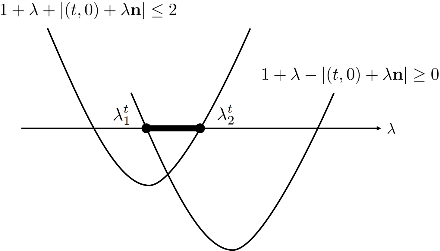
where $\lambda_{1}^{t}$ and $\lambda_{2}^{t}$ are shown in (4.95). Remark that the same argument can be applied for $C(\mathsf{A}^{t\mathbf{y}}:\varrho^{\mathbf{r}_{1}},\varrho^{\mathbf{r}_{2}})$ .

We shall now prove $t_{0}^{\prime}=\inf L\notin L$ . Suppose that $t\in L$ , i.e. $\chi_{incomp}(\mathsf{A}^{t\mathbf{x}}_{D},\mathsf{A}^{t\mathbf{y}}_{D})=2$ . It follows that there exist $\mathbf{r}_{1}$ and $\mathbf{r}_{2}$ in $\partial D$ such that

\displaystyle\left(C(\mathsf{A}_{D}^{t\mathbf{x}}:\varrho^{\mathbf{r}_{1}},\varrho^{\mathbf{r}_{2}})\times C(\mathsf{A}^{t\mathbf{y}}_{D}:\varrho^{\mathbf{r}_{1}},\varrho^{\mathbf{r}_{2}})\right)\cap JM(2:2)=\emptyset.

Denoting $C(\mathsf{A}_{D}^{t\mathbf{x}}:\varrho^{\mathbf{r}_{1}},\varrho^{\mathbf{r}_{2}})$ and $C(\mathsf{A}_{D}^{t\mathbf{y}}:\varrho^{\mathbf{r}_{1}},\varrho^{\mathbf{r}_{2}})$ simply by $X^{t}$ and $Y^{t}$ respectively, we can rewrite it as

X^{t}\times Y^{t}\cap JM(2:2)=\emptyset.

We need the following lemma.

Lemma 4.22.

Let $\delta>0$ . There exists $\Delta>0$ such that for all $\tau\in[0,\Delta]$ and for all $\mathsf{C}\in X^{t-\tau}$ , there exists $\mathsf{A}\in X^{t}$ satisfying

d(\mathsf{C},\mathsf{A}):=\|\mathsf{C}(+)-\mathsf{A}(+)\|<\delta

where $d$ is a metric on $O_{D}(2)$ defined through the operator norm $\|\cdot\|$ on $\mathcal{E}_{D}\simeq O_{D}(2)$ .

Proof.

By its definition, $X^{t}$ is a convex set of $O_{D}(2)$ , and thus for all $\mathsf{E}\in O_{D}(2)$ we can define successfully the distance between $\mathsf{E}$ and $X^{t}$ :

d(\mathsf{E},X^{t})=\min_{\mathsf{F}\in X^{t}}d(\mathsf{E},\mathsf{F}).

In particular, for $\mathsf{E}^{\prime}\in X^{t-\Delta^{\prime}}\subset O_{D}(2)$ with $\Delta^{\prime}>0$ and $\mathsf{E}^{\prime}(+)=\frac{1}{2}(e^{\prime}_{0}\mathbbm{1}+\mathbf{e}^{\prime}\cdot\sigma)$ , it becomes

\displaystyle\begin{aligned} d(\mathsf{E}^{\prime},X^{t})=\min_{\mathsf{F}\in X^{t}}d(\mathsf{E}^{\prime},\mathsf{F})=\min_{\mathsf{F}\in X^{t}}\frac{1}{2}\left(|e^{\prime}_{0}-f_{0}|+|\mathbf{e}-\mathbf{f}|\right),\end{aligned}

(4.97)

where $\mathsf{F}(+)=\frac{1}{2}(f_{0}\mathbbm{1}+\mathbf{f}\cdot\sigma)$ (see (4.92)). Since, in terms of (4.96), $\mathsf{E}^{\prime}\in X^{t-\Delta^{\prime}}$ and $\mathsf{F}\in X^{t}$ imply

(e_{0}^{\prime},\mathbf{e}^{\prime})=(1,t-\Delta^{\prime},0)+\lambda^{\prime}(1,\mathbf{n})

with $\lambda_{1}^{t-\Delta^{\prime}}\leq\lambda^{\prime}\leq\lambda_{2}^{t-\Delta^{\prime}}$ and

(f_{0},\mathbf{f})=(1,t,0)+\lambda(1,\mathbf{n})

with $\lambda_{1}^{t}\leq\lambda\leq\lambda_{2}^{t}$ respectively, (4.97) can be rewritten as

\displaystyle\begin{aligned} 2d(\mathsf{E}^{\prime},X^{t})=\min_{\lambda\in[\lambda_{1}^{t},\lambda_{2}^{t}]}\left(|\lambda^{\prime}-\lambda|+|(-\Delta^{\prime},0)+(\lambda^{\prime}-\lambda)\mathbf{n}|\right).\end{aligned}

It follows that

\displaystyle 2d(\mathsf{E}^{\prime},X^{t})\leq\Delta^{\prime}+\min_{\lambda\in[\lambda_{1}^{t},\lambda_{2}^{t}]}|\lambda^{\prime}-\lambda|(1+|\mathbf{n}|).

(4.98)

Let us evaluate its right hand side. It is easy to see that

\min_{\lambda\in[\lambda_{1}^{t},\lambda_{2}^{t}]}|\lambda^{\prime}-\lambda|=\left\{\begin{aligned} \lambda_{1}^{t}&-\lambda^{\prime}&\quad&(\lambda^{\prime}<\lambda_{1}^{t})\\ &0&\quad&(\lambda_{1}^{t}\leq\lambda^{\prime}\leq\lambda_{2}^{t})\\ \lambda^{\prime}&-\lambda_{2}^{t}&\quad&(\lambda^{\prime}>\lambda_{2}^{t})\end{aligned}\right..

Suppose that $\lambda^{\prime}<\lambda_{1}^{t}$ holds, for example. In this case, because $\lambda_{1}^{t-\Delta^{\prime}}\leq\lambda^{\prime}$ , we can obtain

\lambda_{1}^{t}-\lambda^{\prime}\leq\lambda_{1}^{t}-\lambda_{1}^{t-\Delta^{\prime}}.

In a similar way, it can be demonstrated that

\displaystyle\sup_{\lambda^{\prime}\in[\lambda_{1}^{t-\Delta^{\prime}},\lambda_{2}^{t-\Delta^{\prime}}]}\min_{\lambda\in[\lambda_{1}^{t},\lambda_{2}^{t}]}|\lambda^{\prime}-\lambda|=\max\left\{\lambda_{1}^{t}-\lambda_{1}^{t-\Delta^{\prime}},\ 0,\ \lambda_{2}^{t-\Delta^{\prime}}-\lambda_{2}^{t}\right\}.

By virtue of (4.95), the right hand side converges to 0 as $\Delta^{\prime}\rightarrow 0$ , and thus we can see from (4.98) that

\sup_{\mathsf{E}^{\prime}\in X^{t-\Delta^{\prime}}}d(\mathsf{E}^{\prime},X^{t})\underset{\Delta^{\prime}\to 0}{\longrightarrow}0

It results in that there exists $\Delta>0$ such that for all $\tau\in[0,\Delta]$ ,

\sup_{\mathsf{E}^{\prime}\in X^{t-\tau}}d(\mathsf{E}^{\prime},X^{t})<\delta

holds, that is, $d(\mathsf{C},X^{t})<\delta$ holds for any $\mathsf{C}\in X^{t-\tau}$ . Moreover, because $X^{t}$ is convex, there exists $\mathsf{A}\in X^{t}$ satisfying $d(\mathsf{C},X^{t})=d(\mathsf{C},\mathsf{A})$ , which proves the claim of the lemma.

Note that a similar statement also holds for $Y^{t}$ : there exists $\widetilde{\Delta}>0$ such that for all $\widetilde{\tau}\in[0,\widetilde{\Delta}]$ and for all $\mathsf{D}\in Y^{t-\widetilde{\tau}}$ , there exists $\mathsf{B}\in Y^{t}$ satisfying $d(\mathsf{D},\mathsf{B})<\delta$ . Let $V:=O_{D}(2)\times O_{D}(2)(\simeq\mathcal{E}_{D}\times\mathcal{E}_{D})$ and let $d_{V}$ be a product metric on $V$ defined as

\displaystyle d_{V}\left((\mathsf{A},\mathsf{B}),(\mathsf{C},\mathsf{D})\right)=\max\{d(\mathsf{A},\mathsf{C}),d(\mathsf{B},\mathsf{D})\}.

According to Lemma 4.22 and its $Y^{t}$ -counterpart, if we take $\Delta_{0}=\min\{\Delta,\widetilde{\Delta}\}(>0)$ , then there exists $(\mathsf{A},\mathsf{B})\in X^{t}\times Y^{t}$ for all $(\mathsf{C},\mathsf{D})\in X^{t-\Delta_{0}}\times Y^{t-\Delta_{0}}$ such that $d_{V}((\mathsf{A},\mathsf{B}),(\mathsf{C},\mathsf{D}))<\delta$ . On the other hand, as we have seen, it holds that

X^{t}\times Y^{t}\cap JM(2:2)=\emptyset.

Since $X^{t}\times Y^{t}$ and $JM(2:2)$ are closed in $V$ , and $V$ is a metric space, we can apply Urysohn’s Lemma [153]. It follows that there exists a continuous (in fact uniformly continuous since $V$ is compact) function $f\colon V\to[0,1]$ satisfying $f(U)=0$ for any $U\in X^{t}\times Y^{t}$ and $f(W)=1$ for any $W\in JM(2:2)$ . The uniform continuity of $f$ implies that for some $\varepsilon\in(0,1)$ , there is $\delta>0$ such that

\displaystyle\begin{aligned} d_{V}\left((\mathsf{E}^{\prime},\mathsf{F}^{\prime}),(\mathsf{E},\mathsf{F})\right)<\delta\ \Rightarrow\ \left|f\left((\mathsf{E}^{\prime},\mathsf{F}^{\prime})\right)-f\left((\mathsf{E},\mathsf{F})\right)\right|<\varepsilon\end{aligned}

(4.99)

holds for any $(\mathsf{E},\mathsf{F})\in V$ . For this $\delta$ , we can apply the argument above: we can take $\Delta_{0}>0$ such that for any $(\mathsf{C},\mathsf{D})\in X^{t-\Delta_{0}}\times Y^{t-\Delta_{0}}$ , there exists $(\mathsf{A},\mathsf{B})\in X^{t}\times Y^{t}$ satisfying $d_{V}((\mathsf{A},\mathsf{B}),(\mathsf{C},\mathsf{D}))<\delta$ . Because $f((\mathsf{A},\mathsf{B}))=0$ , we have $f((\mathsf{C},\mathsf{D}))<\varepsilon<1$ (see (4.99)), and thus $(\mathsf{C},\mathsf{D})\notin JM(2:2)$ . It indicates that $X^{t-\Delta_{0}}\times Y^{t-\Delta_{0}}\cap JM(2:2)=\emptyset$ , that is, there is $\Delta_{0}>0$ for any $t\in L$ satisfying $t-\Delta_{0}\in L$ . Therefore, $t_{0}^{\prime}=\inf L\notin L$ can be concluded.

Chapter 5 Thermodynamical entropy of mixing in regular polygon theories

The concept of entropy plays an important role in thermodynamics [154, 155]. It is possible to calculate the thermodynamical entropy of a mixture of classically different kinds of particles (such as a mixture of nitrogens and oxygens), and similar ideas were applied by von Neumann to the case where the system was composed of particles with different quantum internal states [5]. Similarly to the previous parts, it is expected that generalizing the notion of entropy to GPTs will help us to understand how entropy can affect our world. In fact, there have been researches which aim to introduce and investigate the concept of entropy in GPTs from informational perspectives [62, 156, 157, 158]. In those researches, some kinds of entropy were defined in all theories of GPTs and their information-theoretical properties were investigated. Meanwhile, there have been also researches referring to the thermodynamical entropy in terms of the microcanonical or canonical formulation in GPTs [159, 160], and researches referring to the thermodynamical entropy of mixing in GPTs [118, 161]. However, in those works, the entropy was only defined in or applied to some restricted theories of GPTs with special assumptions such as the existence of a spectral decomposition for any state into perfectly distinguishable pure states. In particular, it can be found that regular polygon theories do not always satisfy those assumptions, and thus entropy in regular polygon has never been investigated although they can be regarded as intermediate theories of a classical trit system and a qubit-like system, where entropy is defined successfully. It seems natural to ask how entropy of mixing behaves in regular polygon theories.

In this part, we consider thermodynamical entropy of mixing in regular polygon theories. It is proven that the operationally natural thermodynamical entropy of a mixture of ideal particles with different internal states described by a regular polygon theory exists if and only if the state space of theory is triangle-shaped or disc-shaped, i.e., the theory is either classical or quantum-like. More precisely, we demonstrate that the thermodynamical entropy of mixing satisfying conditions imposed in [118], where the concrete operational construction of the entropy was given as von Neumann did under the assumption of the existence of semipermeable membranes, does not exist in all the regular polygon theories except for classical and quantum-like ones.

This part is organized as follows. In Section 12, we present a generalization of thermodynamically natural entropy of mixing in GPTs. We will see that the notion of perfect distinguishability plays an important role to define entropy also in GPTs. Then we demonstrate our main theorem and its proof in Section 13.

12 Entropy of mixing in GPTs

In this section, we introduce the thermodynamically consistent definition of entropy of mixing in GPTs based on the notion of perfect distinguishability.

12.1 Perfect distinguishablity for regular polygon theories

We recall that a family of states $\{\omega_{i}\}_{i}$ is called perfectly distinguishable if there exists an observable $\{e_{i}\}_{i}$ such that $e_{i}(\omega_{j})=\delta_{ij}$ . Let us characterize perfectly distinguishable states in regular polygon theories. We first consider the regular polygon theory with $n$ sides, where $n$ is an even number greater than two. Calculating the Euclidean inner product (denoted by $(\cdot,\cdot)$ here) of pure effects and pure states in Subsection 5.3, we obtain

\displaystyle\left(e^{n}_{i},\ \omega^{n}_{i}\right)=\left(e^{n}_{i},\ \omega^{n}_{i-1}\right)=1,\ \ (e^{n}_{i},\ \omega^{n}_{i+\frac{n}{2}-1})=(e^{n}_{i},\ \omega^{n}_{i+\frac{n}{2}})=0.

These equations indicate that any state in $\Omega_{n}^{[i-1,\ i]}$ is perfectly distinguishable from any state in $\Omega_{n}^{[i+\frac{n}{2}-1,\ i+\frac{n}{2}]}$ , where we define

\displaystyle\Omega_{n}^{[k-1,\ k]}=\{\omega\in\Omega_{n}\mid\omega=p\omega^{n}_{k-1}+(1-p)\omega^{n}_{k},\ 0\leq p\leq 1\},

since the measurement $\{e^{n}_{i},\ u-e^{n}_{i}\}$ distinguishes perfectly those two states. For odd $n\ (\geq 3)$ , we obtain

\displaystyle\left(e^{n}_{i},\ \omega^{n}_{i}\right)=1,\ \ (e^{n}_{i},\ \omega^{n}_{i+\frac{n-1}{2}})=(e^{n}_{i},\ \omega^{n}_{i+\frac{n+1}{2}})=0.

Hence $\omega^{n}_{i}$ and an arbitrary state in $\Omega_{n}^{[i+\frac{n-1}{2},\ i+\frac{n+1}{2}]}$ are perfectly distinguishable. Finally, when $n=\infty$ ,

\displaystyle\left(e^{\infty}_{\theta},\ \omega^{\infty}_{\theta}\right)=1,\ \ (e^{\infty}_{\theta},\ \omega^{\infty}_{\theta+\pi})=0.

hold, so there is only one perfectly distinguishable state for each pure state (see Figure 10).

12.2 Entropy of mixing in GPTs

In this part, we consider the thermodynamical entropy of mixing in a system composed of ideal gases with different internal degrees of freedom described by a GPT. In thermodynamics, it is well known that a mixture of several classically distinct ideal gases, such like a mixture of ideal hydrogens and nitrogens, causes an increase of entropy. The amount of increase by the mixture can be calculated under the assumption of the existence of semipermeable membranes which distinguish perfectly those particles. We assume in a similar way that if the internal states $\omega_{1},\omega_{2},\cdots,\omega_{l}$ described by a GPT are perfectly distinguishable, then there exist semipermeable membranes which can identify completely a state among them without disturbing every $\omega_{j}$ $(j=1,2,\cdots,l)$ .

We consider ideal gases in thermal equilibrium with its temperature $T$ , volume $V$ , and $N$ particles, and do not focus on the mechanical part of the particles in the following. All of these $N$ particles are in the same internal state $\omega=\sum_{i=1}^{l}p_{i}\omega_{i}$ , where $\{\omega_{1},\omega_{2},\cdots,\omega_{l}\}$ is a perfectly distinguishable set of states, and $\forall i,\ p_{i}\geq 0,\ \mbox{and}\ \sum_{i=1}^{l}p_{i}=1$ , meaning that this system is composed of the mixture of $l$ different kinds of particles whose internal states are $\omega_{1},\omega_{2},\cdots,\omega_{l}$ with a probability weight $\{p_{1},p_{2},\cdots,p_{l}\}$ . We note again that in this chapter, classical species of particles are also regarded as the internal states of them. In classical thermodynamics, thermodynamical entropy is calculated by constructing concrete thermodynamical operations such as isothermal or adiabatic quasistatic operations. We follow this doctrine of thermodynamics also in GPTs that thermodynamical entropy, especially thermodynamical entropy of mixing, should be operationally-derived quantity. In fact, as shown in [118], our assumption of the existence of semipermeable membranes makes it possible to realize concrete thermodynamical operations to calculate the thermodynamical entropy of mixing of the system mentioned above in the same way as von Neumann did when the internal degrees of freedom were quantum [5]. Strictly speaking, it has been demonstrated operationally in [118] that the thermodynamical entropy of mixing in the system is

S(\omega)=\sum_{i=1}^{l}p_{i}S(\omega_{i})-\sum_{i=1}^{l}p_{i}\log p_{i}\ ,

(5.1)

where $S(\sigma)$ means the per-particle thermodynamical entropy of mixing in the system which consists of particles in the same state $\sigma$ , and we set the Boltzmann constant $k_{\mathrm{B}}=1$ (also $0\log 0=0$ ). In the process of deriving (5.2), the additivity and extensivity of the thermodynamical entropy, and the continuity of $S$ with respect to states are assumed. The latter one is needed in order to apply (5.2) to arbitrary states with an arbitrary probability weight, while its operational derivation has been given only when each $p_{i}N$ is the number of particles in the state $\omega_{i}$ and thus each $p_{i}$ is rational. We impose additional assumption that the entropy of any pure state is equal to zero, that is, $S(\sigma)=0$ whenever $\sigma$ is a pure state.

13 Main result

Our main result is in the following form.

Theorem 5.1.

Consider a system in thermal equilibrium composed of ideal gases whose internal states are described an element of the state space $\Omega_{n}$ of the regular polygon theory with $n$ sides ( $n\geq 3$ ). The (per-particle) thermodynamical entropy of mixing $S:\Omega_{n}\rightarrow\mathbb{R}$ satisfying

\displaystyle S(\omega)=\sum_{i=1}^{l}p_{i}S(\omega_{i})-\sum_{i=1}^{l}p_{i}\log p_{i},

(5.2)

where $\{\omega_{i}\}_{i}$ is a family of perfectly distinguishable states, exists if and only if $n=3\ \mbox{or}\ \infty$ , that is, the state space is classical or quantum-like.

Proof.

For $n=3$ , because it is a classical system, any $\omega\in\Omega_{3}$ is decomposed uniquely into perfectly distinguishable pure states as $\omega=p\omega_{0}^{3}+q\omega_{1}^{3}+(1-p-q)\omega_{2}^{3}$ , where $\omega_{i}^{3}\ (i=0,1,2)$ are the three pure states in $\Omega_{3}$ and $\{p,q,1-p-q\}$ is a probability weight. In this settings, we define $S$ as

\displaystyle S(\omega)=-p\log p-q\log q-(1-p-q)\log(1-p-q).

This $S$ gives the well-defined entropy satisfying (5.2). Similarly, when $n=\infty$ , any state has only one decomposition into perfectly distinguishable (pure) states except for the central state of $\Omega_{\infty}$ (the maximally mixed state). For states that are not maximally mixed, we define $S$ as

\displaystyle S(\omega)=H(p),

where we decompose a non-maximally-mixed $\omega\in\Omega_{\infty}$ as $\omega=p\omega_{\theta}^{\infty}+(1-p)\omega_{\theta+\pi}^{\infty}\ (0\leq p\leq 1)$ and $H(p)=-p\log p-(1-p)\log(1-p)$ is the 1-bit Shannon entropy. We can apply this $S$ to the maximally mixed state, for the probability weight does not depend on the way of decompositions and they are always $\{\frac{1}{2},\frac{1}{2}\}$ . Therefore, we can define successfully the thermodynamical entropy $S$ which meets (5.2) for $n=3,\infty$ . In the following, we prove the only if part.

The case when $n=4$ was proven in [118], so we only consider $n\geq 5$ . At first, we assume $n$ is an even number, and consider the state $\omega_{\mathrm{P}}$ represented in Figure 11, that is,

\displaystyle\omega_{\mathrm{P}}=\frac{y}{x+y}\omega_{i}^{n}+\frac{x}{x+y}\omega_{i+\frac{n}{2}}^{n}=\frac{t}{s+t}\omega_{i+1}^{n}+\frac{s}{s+t}\omega_{i+\frac{n}{2}+2}^{n},

where $x,y,s,t$ are all nonnegative, and $x\leq y$ and $s\leq t$ as shown in Figure 11. Note that $\{\omega_{i}^{n},\ \omega_{i+\frac{n}{2}}^{n}\}$ and $\{\omega_{i+1}^{n},\ \omega_{i+\frac{n}{2}+2}^{n}\}$ are two perfectly distinguishable pairs of pure states. From the observations in the previous section, we obtain two forms of the thermodynamical entropy of mixing:

S(\omega_{\mathrm{P}})=H\left(\frac{x}{x+y}\right)=H\left(\frac{s}{s+t}\right),

(5.3)

which means

\displaystyle\frac{x}{x+y}=\frac{s}{s+t}

because $x\leq y$ and $s\leq t$ . On the other hand, applying sine theorem to Figure 11 we can see that

\displaystyle\frac{x}{\sin(\frac{\pi}{2}-\frac{2\pi}{n})}=\frac{s}{\sin(\frac{\pi}{2}-\frac{\pi}{n})},\ \ \frac{y}{\sin(\frac{\pi}{2}-\frac{\pi}{n})}=\frac{t}{\sin(\frac{\pi}{2}-\frac{2\pi}{n})},

namely

\displaystyle\frac{s}{s+t}=\frac{x}{x+\left(\frac{\cos\frac{2\pi}{n}}{\cos\frac{\pi}{n}}\right)^{2}\ y}

holds. It follows from these two equations that

\left(\frac{\cos\frac{2\pi}{n}}{\cos\frac{\pi}{n}}\right)^{2}=1,

and because for even $n$ , this equation holds if and only if $n=\infty$ ( $\cos(\frac{\pi}{n})=1$ ), the entropy in (5.3) has been proven to be ill-defined.

Next, we consider the case where $n$ is an odd number greater than three. We define the state $\omega_{\mathrm{A}}$ as $\omega_{\mathrm{A}}=\frac{1}{2}(\omega_{i+\frac{n-1}{2}}^{n}+\omega_{i+\frac{n+1}{2}}^{n})$ , and consider two states $\omega_{\mathrm{Q}}$ and $\omega_{\mathrm{R}}$ shown in Figure 12, where $j=\frac{n+1}{4}\ \mbox{or}\ \frac{n-1}{4}$ corresponding to the case where $n\equiv 3$ or $n\equiv 1$ (mod 4) respectively.

Note that $\{\omega_{i}^{n},\ \omega_{\mathrm{A}}\}$ and $\{\omega_{i+1}^{n},\ \omega_{i+\frac{n+1}{2}}^{n}\}$ in Figure 12, and $\{\omega_{i+j}^{n},\ \omega_{i+(n-j)}^{n}\}$ in Figure 12 are perfectly distinguishable pairs of states. Then

\displaystyle S(\omega_{\mathrm{Q}})=\frac{p}{p+q}S(\omega_{\mathrm{A}})+H\left(\frac{p}{p+q}\right)=H\left(\frac{u}{u+v}\right),

and

\displaystyle S(\omega_{\mathrm{R}})=\frac{w}{w+z}S(\omega_{\mathrm{A}})+H\left(\frac{w}{w+z}\right)=H\left(\frac{1}{2}\right)

hold. We assume that the entropies of the two states $\omega_{\mathrm{Q}},\ \omega_{\mathrm{R}}$ are well-defined (so is $\omega_{\mathrm{A}}$ ). Then

	$\displaystyle S(\omega_{\mathrm{A}})$	$\displaystyle=\frac{p+q}{p}\left\{H\left(\frac{u}{u+v}\right)-H\left(\frac{p}{p+q}\right)\right\}$		(5.4)
		$\displaystyle=\frac{w+z}{w}\left\{H\left(\frac{1}{2}\right)-H\left(\frac{w}{w+z}\right)\right\}$		(5.5)

holds. Let us give the explicit expressions of (5.5). From Figure 13, we obtain

\displaystyle\frac{u}{v}=\frac{r_{n}\sin(\frac{n-2}{n}\pi)}{r_{n}\sin\frac{\pi}{n}}=\frac{\sin\frac{2\pi}{n}}{\sin\frac{\pi}{n}}=2\cos\frac{\pi}{n},

and by sine theorem,

\displaystyle\frac{p}{\sin(\frac{\pi}{2}-\frac{\pi}{2n})}=\frac{u}{\sin(\frac{\pi}{2}-\frac{\pi}{n})},\ \ q=v\cos\frac{3\pi}{2n}

hold. Therefore,

	$\displaystyle\frac{q}{p}$	$\displaystyle=\frac{v}{u}\cdot\frac{\cos\frac{\pi}{n}\cdot\cos\frac{3\pi}{2n}}{\cos\frac{\pi}{2n}}$
		$\displaystyle=\frac{\cos\frac{3\pi}{2n}}{2\cos\frac{\pi}{2n}}$
		$\displaystyle=\frac{1}{2}\left(4\cos^{2}\frac{\pi}{2n}-3\right)$
		$\displaystyle=\frac{1}{2}\left(2\cos\frac{\pi}{n}-1\right).$

On the other hand, from Figure 12, we obtain

\displaystyle\begin{aligned} \frac{z}{w}&=\frac{2r_{n}\cos^{2}\frac{\pi}{2n}-2r_{n}\cos^{2}(\frac{n-2j}{2n}\pi)}{2r_{n}\cos^{2}(\frac{n-2j}{2n}\pi)}\\ &=\frac{\cos^{2}\frac{\pi}{2n}-\sin^{2}\frac{j\pi}{n}}{\sin^{2}\frac{j\pi}{n}}\ \ \ \ \mbox{for}\ \ j=\frac{n\pm 1}{4}.\end{aligned}

(5.6)

Since

$\displaystyle\sin^{2}\frac{j\pi}{n}$	$\displaystyle=\frac{1}{2}\left(1-\cos\frac{2j\pi}{n}\right)$	(5.7)
	$\displaystyle=\frac{1}{2}\left(1-\cos\frac{(n\pm 1)\pi}{2n}\right)$
	$\displaystyle=\frac{1}{2}\left(1\pm\sin\frac{\pi}{2n}\right),$

the equation above can be written as

	$\displaystyle\frac{z}{w}$	$\displaystyle=\frac{2(1+\sin\frac{\pi}{2n})(1-\sin\frac{\pi}{2n})-(1\pm\sin\frac{\pi}{2n})}{1\pm\sin\frac{\pi}{2n}}$
		$\displaystyle=1\mp 2\sin\frac{\pi}{2n},$

where the double sign corresponds to the ones in (5.6) and (5.7), and the upper and lower sign correspond to the case of $n\equiv 3$ and $n\equiv 1$ (mod 4) respectively. Substituting these results to (5.4) and (5.5), we obtain

	$\displaystyle S(\omega_{\mathrm{A}})$	$\displaystyle=\left(\frac{2\cos\frac{\pi}{n}+1}{2}\right)\left\{H\left(\frac{1}{2\cos\frac{\pi}{n}+1}\right)-H\left(\frac{2}{2\cos\frac{\pi}{n}+1}\right)\right\}$
		$\displaystyle=\left(2\mp 2\sin\frac{\pi}{2n}\right)\left\{H\left(\frac{1}{2}\right)-H\left(\frac{1}{2\mp 2\sin\frac{\pi}{2n}}\right)\right\}.$

By letting $\alpha=\sin\frac{\pi}{2n}$ , it can be rewritten as

	$\displaystyle S(\omega_{\mathrm{A}})$	$\displaystyle=2\alpha^{2}\log 2+\frac{1-4\alpha^{2}}{2}\log(1-4\alpha^{2})-(1-2\alpha^{2})\log(1-2\alpha^{2})$		(5.8)
		$\displaystyle=(1\mp 2\alpha)\log(1\mp 2\alpha)-(2\mp 2\alpha)\log(1\mp\alpha),$		(5.9)

where the upper and lower signs correspond to the case of $n\equiv 3$ and $n\equiv 1$ (mod 4) respectively. The differences between (5.8) and (5.9) in the case of $n\equiv 3$ and $n\equiv 1$ are displayed in Figures 14 and 14 respectively, and we can see that the two forms of $S(\omega_{\mathrm{A}})$ shown in (5.8) and (5.9) do not agree with each other. In conclusion, it has been proven that if $n\neq 3,\ \infty$ , then there exists some state whose thermodynamical entropy of mixing is ill-defined.

We can see the ill-defined values of entropy become well-defined if $n=3,\ \infty$ in our proof. For example, when $n$ is an odd number, $\alpha=\sin\frac{\pi}{2n}$ is equal to $\frac{1}{2}$ or $0$ if $n$ is equal to three or infinite, respectively, and two values (5.8) and (5.9) coincide with each other in these cases (see Figure 14).

Remark 5.2.

Similar results were obtained in [118], where it was assumed that any state could be represented as a convex combination of perfectly distinguishable pure states. However, a state of a regular polygon theory is not always represented by a convex combination of perfectly distinguishable pure states. For instance, we can see from Figure 10 that the state $\omega_{\mathrm{A}}$ in Figure 12 or Figure 12 can not be decomposed into perfectly distinguishable pure states. Thus regular polygon theories generally do not satisfy the assumption in the previous study [118], and our result is the one about the exsistence of well-defined thermodynamical entropy in such a broader class of theories where “spectral decompositions” of states are not generally possible.

Chapter 6 Summary

In this thesis, we have studied the notion of uncertainty in quantum theory via convexity. We focused on three expressions of uncertainty: uncertainty relations, incompatibility, and thermodynamical entropy. Our establishments were based on the idea that to see quantum uncertainty from a broader point of view makes it possible to understand its essence. In fact, in each chapter, we considered uncertainty relations and thermodynamical entropy in a broader class of theories than quantum theory, and investigated quantum incompatibility, which is a broader notion than uncertainty.

In Chapter 2, we introduced the mathematical framework of GPTs. We saw that GPTs are constructed by requiring only primitive convexity originating from probability mixtures, and thus in this sense, they are the most general description of nature (in particular, broader than quantum theory). There were proven that GPTs can be expressed mathematically in terms of ordered Banach spaces, and that it indeed reproduce the usual formulation of quantum theory.

In Chapter 3, several generalizations of uncertainty relations such as entropic uncertainty relations were considered in a class of GPTs which can be considered as generalized theories of quantum theory. It was revealed that similar quantitative relations between preparation and measurement uncertainty to quantum case hold also in GPTs although only theories with transitivity and self-duality with respect to a certain inner product were considered. We also gave concrete calculations of our results for regular polygon theories. What is also specific to theorems is that they were obtained without considering entanglement or even composite systems while the quantum results of the previous studies were based on the “ricochet” property of maximally entangled states. It may be indicated that some of the characteristics of quantum theory can be obtained without entanglement. Future research should reveal the relations between the maximal entanglement and self-duality, which will be a key to generalizing our theorems to infinite-dimensional cases (remember that the maximally entangled states cannot be defined in infinite-dimensional quantum theories such as $\mathcal{H}=L^{2}(\mathbb{R})$ ). To find information-theoretic applications of our results is also left for future work.

In Chapter 4, we focused on incompatibility in quantum theory, and introduced the notions of compatibility and incompatibility dimensions for collections of quantum devices. They describe the minimum number of states which are needed to detect incompatibility and the maximum number of states on which incompatibility vanishes, respectively. We have not only presented general properties of those quantities but also examined concrete behaviors of them for a pair of unbiased qubit observables. We have proven that even for this simple pair of incompatible observables there exist two types of incompatibility with different incompatibility dimensions which cannot be observed if we focus only on robustness of incompatibility under noise. We expect that it is possible to apply this difference to some quantum protocols such as quantum cryptography. Future work will be needed to investigate whether similar results can be obtained for observables in higher dimensional Hilbert space or other quantum devices. As the definitions apply to devices in GPTs, an interesting task is further to see how quantum incompatibility dimension differs from incompatibility dimension in general.

In Chapter 5, we returned to GPTs and considered theremodynamical entropy in regular polygon theories. We showed that only classical and quantum-like theories (i.e. the triangle and disc theories respectively) allow the operationally natural entropy to be consistent. Further research is required to reveal if we can obtain the same results in higher dimensional cases. Moreover, the proof of our main theorem indicates that the entropy discussed above is defined successfully in other theories where the probability coefficients obtained when a state is decomposed into perfectly distinguishable states are unique even though the state space is neither classical nor quantum. This means that we need to impose additional conditions on the entropy to remove those“unreasonable” theories, which is also a future problem.

Acknowledgments

I would like to, first and foremost, thank my supervisor Takayuki Miyadera. Since I became his student in 2016, he has taught me many interesting things on quantum theory to lead me to the study of quantum foundations. Topics such as quantum uncertainty or incompatibility are examples of those things, and they are now the main interest of my research. His insightful guidance, not only as a great researcher but also as a great person, has helped and will help me a lot in my research and daily life. Nothing in my nine-year college experience makes me more proud of than being his student and able to learn from him. I also would like to thank my collaborator Teiko Heinosaari. I feel very honored to have worked with such a great person and exhibit our results in my PhD thesis. I cannot miss thanking all members of my laboratory, especially Kenzo Ogure, Ikko Hamamura, and Kazuki Yamaga, for their fruitful help in my study. This research has been supported by JSPS KAKENHI Grant Number JP21J10096, and I also acknowledge the JSPS Research Fellowship for Young Scientists.

Finally, I would like to express my thanks to my family and friends. I am grateful to my parents for giving me birth with so good a constitution that I can stay healthy in everyday life. I also thank my friends for their encouragement and support. They are all great persons, and examples for me. I have learned from them what are the most important things in life. Those things are always within my mind, and are the principles that guide my life. My deepest gratitude is expressed to my grandparents. The greatest thing in my life is that they are my grandparents. We live so far that we cannot often see each other, but I always feel their love supporting and encouraging me in my daily life. I hope that my accomplishment of this PhD study will be their pleasure.

Appendix

A Proof of Proposition 2.53

In this part, we give a proof of Proposition 2.53. We need the following proposition, which holds without the assumption of the transitivity of $\Omega$ .

Proposition A.1.

For a state space $\Omega$ , define a linear map $P_{M}\colon V\rightarrow V$ by

P_{M}x=\int_{GL(\Omega)}Tx\ d\mu(T).

Then $P_{M}$ is an orthogonal projection with respect to the inner product $\langle\cdot,\cdot\rangle_{GL(\Omega)}$ , i.e.

P_{M}=P_{M}^{2}\quad\mbox{and}\quad\langle P_{M}x,\ y\rangle_{GL(\Omega)}=\langle x,\ P_{M}y\rangle_{GL(\Omega)}\ \ \mbox{for all}\ x,y\in V.

Proof.

We denote the inner product $\langle\cdot,\cdot\rangle_{GL(\Omega)}$ simply by $\langle\cdot,\cdot\rangle$ in this proof.

Let $V_{M}:=\{x\in V\mid Tx=x\ \mbox{for all}\ T\in GL(\Omega)\}$ be the set of all fixed points with respect to $GL(\Omega)$ . Then it is easy to see that $P_{M}x_{M}=x_{M}$ for any $x_{M}\in V_{M}$ and $V_{M}=ImP_{M}$ (in particular $V_{M}$ is a subspace of $V$ ). Therefore,

P_{M}^{2}x=P_{M}(P_{M}x)=P_{M}x

holds for any $x\in V$ , and thus $P_{M}^{2}=P_{M}$ . On the other hand, we can observe

$\displaystyle\langle P_{M}x,\ y\rangle$	$\displaystyle=\int_{GL(\Omega)}d\mu(T)\ (TP_{M}x,\ Ty)_{E}$
	$\displaystyle=\int_{GL(\Omega)}d\mu(T)\ (P_{M}x,\ Ty)_{E}$
	$\displaystyle=\int_{GL(\Omega)}d\mu(T)\ \left(\int_{GL(\Omega)}d\mu(S)Sx,\ Ty\right)_{E}.$	(A.1)

Let us fix an orthonormal basis $\{w_{i}\}_{i=1}^{N+1}$ of $V$ compatible with the standard Euclidean inner product of $V$ , i.e.

(w_{i},\ w_{j})_{E}=\delta_{ij}.

We can consider representing the vector $\int_{GL(\Omega)}d\mu(S)Sx\in V$ by means of the orthonormal basis $\{w_{i}\}_{i}$ as

\int_{GL(\Omega)}d\mu(S)Sx=\sum_{i}\left(w_{i},\ \int_{GL(\Omega)}d\mu(S)Sx\right)_{E}w_{i}.

In fact, the “ $i$ th-element” $\left(w_{i},\ \int_{GL(\Omega)}d\mu(S)Sx\right)_{E}$ is given by (see [162] for more details)

\left(w_{i},\ \int_{GL(\Omega)}d\mu(S)Sx\right)_{E}=\int_{GL(\Omega)}d\mu(S)\ (w_{i},\ Sx)_{E}.

It results in

	$\displaystyle\left(\int_{GL(\Omega)}d\mu(S)Sx,\ Ty\right)_{E}$	$\displaystyle=\sum_{i}\left[\int_{GL(\Omega)}d\mu(S)(w_{i},\ Sx)_{E}\right](w_{i},Ty)_{E}$
		$\displaystyle=\int_{GL(\Omega)}d\mu(S)\left[\sum_{i}(Sx,\ w_{i})_{E}(w_{i},Ty)_{E}\right]$
		$\displaystyle=\int_{GL(\Omega)}d\mu(S)(Sx,\ Ty)_{E}.$

Therefore, we obtain

		$\displaystyle\int_{GL(\Omega)}d\mu(T)\ \left(\int_{GL(\Omega)}d\mu(S)Sx,\ Ty\right)_{E}$
		$\displaystyle\qquad\qquad\qquad\qquad=\int_{GL(\Omega)}d\mu(T)\ \left[\int_{GL(\Omega)}d\mu(S)\ (Sx,\ Ty)_{E}\right]$
		$\displaystyle\qquad\qquad\qquad\qquad=\int_{GL(\Omega)}d\mu(S)\ \left[\int_{GL(\Omega)}d\mu(T)\ (Sx,\ Ty)_{E}\right]$
		$\displaystyle\qquad\qquad\qquad\qquad=\int_{GL(\Omega)}d\mu(S)\ \left(Sx,\ \int_{GL(\Omega)}d\mu(T)Ty\right)_{E},$

where we use Fubini’s theorem for the finite Haar measure $\mu$ on $GL(\Omega)$ . We can conclude together with (A.1) that

\langle P_{M}x,\ y\rangle=\langle x,\ P_{M}y\rangle

holds. $\Box$

Proposition A.1 enables us to give an orthogonal decomposition of a vector $x\in V$ such that

x=(\mathbbm{1}-P_{M})x+P_{M}x,

(A.2)

where $(\mathbbm{1}-P_{M})x\in V_{M}^{\perp}$ and $P_{M}x\in V_{M}$ . When the transitivity of $\Omega$ is assumed, (A.2) is reduced to Proposition 2.53.

Proposition 2.53.

x\in\mathit{aff}(\Omega)\iff x=\sum_{l=1}^{N}a_{l}v_{l}+v_{N+1}=\sum_{l=1}^{N}a_{l}v_{l}+\omega_{M}\ (a_{1},\cdots,a_{N}\in\mathbb{R}).

Proof.

Since we set $\mathrm{dim}\mathit{aff}(\Omega)=N$ , there exists a set of $N$ linear independent vectors $\{v_{l}\}_{l=1}^{N}\subset[\mathit{aff}(\Omega)-\omega_{M}]$ which forms a basis of the $N$ -dimensional vector subspace $[\mathit{aff}(\Omega)-\omega_{M}]\subset V$ , and we can assume by taking an orthonormalization that they are orthonormal with respect to the inner product $\langle\cdot,\cdot\rangle$ . Hence $x\in\mathit{aff}(\Omega)$ if and only if it is represented as

x=\sum_{l=1}^{N}a_{l}v_{l}+\omega_{M}\quad(a_{1},\cdots,a_{N}\in\mathbb{R}).

(A.3)

Moreover, because of the definition of $\mathit{aff}(\Omega)$ , for every $v_{l}\in[\mathit{aff}(\Omega)-\omega_{M}]$ there exist $k\in\mathbb{N}$ , real numbers $\{b_{i}\}_{i=1}^{k}$ satisfying $\sum_{i=1}^{k}b_{i}=1$ , and states $\{\omega_{i}\}_{i=1}^{k}$ such that $v_{l}=\sum_{i=1}^{k}b_{i}\omega_{i}-\omega_{M}$ . By means of Proposition 2.52, we obtain for all $l=1,2,\cdots,N$

	$\displaystyle P_{M}v_{l}$	$\displaystyle=\sum_{i=1}^{k}b_{i}P_{M}\omega_{i}-P_{M}\omega_{M}$
		$\displaystyle=\sum_{i=1}^{k}b_{i}\omega_{M}-\omega_{M}=0.$		(A.4)

Therefore, because of Proposition A.1

	$\displaystyle\langle\omega_{M},\ v_{l}\rangle$	$\displaystyle=\langle P_{M}\omega_{M},\ v_{l}\rangle$
		$\displaystyle=\langle\omega_{M},\ P_{M}v_{l}\rangle$
		$\displaystyle=0$

holds for all $l=1,2,\cdots,N$ , and we can conclude together with the unit norm of $\omega_{M}$ that $\{v_{1},\cdots,v_{N},\omega_{M}\}$ in (A.3) forms an orthonormal basis of the $(N+1)$ -dimensional vector space $V$ with respect to $\langle\cdot,\cdot\rangle$ and Proposition 2.53 is proven (we can also find that (A.3) corresponds to (A.2)).

Appendix 6.B Proof of Proposition 2.55

In this part, we prove Proposition 2.55. As we have so far, we let $\Omega$ be a state space, $V_{+}$ be the positive cone generated by $\Omega$ , and $GL(\Omega)$ be the set of all state automorphisms on $\Omega$ in the following.

Lemma B.1.

$V_{+\langle\cdot,\cdot\rangle_{GL(\Omega)}}^{*int}$ is a $GL(\Omega)$ -invariant set. That is, $TV_{+\langle\cdot,\cdot\rangle_{GL(\Omega)}}^{*int}=V_{+\langle\cdot,\cdot\rangle_{GL(\Omega)}}^{*int}$ for all $T\in GL(\Omega)$ .

Proof.

Let $w\in V_{+\langle\cdot,\cdot\rangle_{GL(\Omega)}}^{*int}$ . It holds that $\langle w,v\rangle_{GL(\Omega)}\geq 0$ for all $v\in V_{+}$ . Because any $T\in GL(\Omega)$ is an orthogonal transformation with respect to $\langle\cdot,\cdot\rangle_{GL(\Omega)}$ , we obtain

\langle Tw,v\rangle_{GL(\Omega)}=\langle w,T^{-1}v\rangle_{GL(\Omega)}\geq 0

for all $v\in V_{+}$ . Therefore, $TV_{+\langle\cdot,\cdot\rangle_{GL(\Omega)}}^{*int}\subset V_{+\langle\cdot,\cdot\rangle_{GL(\Omega)}}^{*int}$ holds, and a similar argument for $T^{-1}\in GL(\Omega)$ proves the lemma.

Lemma B.2.

Let $(\cdot,\cdot)$ be an arbitrary inner product on $V$ . $V_{+}$ is self-dual if and only if there exists a linear map $J\colon V\to V$ such that $J$ is strictly positive with respect to $(\cdot,\cdot)$ , i.e. $(x,Jy)=(Jx,y)$ for all $x,y\in V$ and $(x,Jx)>0$ for all $x\in V$ , and $J(V_{+})=V^{*int}_{+(\cdot,\cdot)}$ .

Proof.

If part: We introduce an inner product $(\cdot,\cdot)_{J}=(\cdot,J\cdot)$ . $V_{+(\cdot,\cdot)_{J}}^{*int}$ is written as

	$\displaystyle V_{+(\cdot,\cdot)_{J}}^{*int}$	$\displaystyle=\{v\mid(v,w)_{J}\geq 0,\ ^{\forall}w\in V_{+}\}$
		$\displaystyle=\{v\mid(v,Jw)\geq 0,\ ^{\forall}w\in V_{+}\}$
		$\displaystyle=\{v\mid(Jv,w)\geq 0,\ ^{\forall}w\in V_{+}\}.$

Thus $v\in V_{+(\cdot,\cdot)_{J}}^{*int}$ is equivalent to $Jv\in V_{+(\cdot,\cdot)}^{*int}$ . It concludes $V_{+(\cdot,\cdot)_{J}}^{*int}=J^{-1}(V_{+(\cdot,\cdot)}^{*int})=V_{+}$ .
Only if part: Let $V_{+}$ be self-dual with respect to an inner product $\langle\cdot,\cdot\rangle$ . There exists some $K\colon V\to V$ strictly positive with respect to $(\cdot,\cdot)$ such that $\langle\cdot,\cdot\rangle=(\cdot,K\cdot)$ . We obtain

	$\displaystyle V_{+}=V_{+\langle\cdot,\cdot\rangle}^{*int}$	$\displaystyle=\{v\|\ \langle v,w\rangle\geq 0,\ ^{\forall}w\in V_{+}\}$
		$\displaystyle=\{v\|\ (v,Kw)\geq 0,\ ^{\forall}w\in V_{+}\}$
		$\displaystyle=\{v\|\ (Kv,w)\geq 0,\ ^{\forall}w\in V_{+}\}$

Thus $v\in V_{+}=V_{+\langle\cdot,\cdot\rangle}^{*int}$ is equivalent to $Kv\in V^{*int}_{+(\cdot,\cdot)}$ , i.e. $KV_{+}=V^{*int}_{+(\cdot,\cdot)}$ . Define $J=K$ .

In Lemma B.2, we gave a necessary and sufficient condition for $V_{+}$ with an inner product $(\cdot,\cdot)$ to be self-dual. The condition was the existence of a strictly positive map $J$ satisfying $J(V_{+})=V_{+(\cdot,\cdot)}^{*int}$ . This map $J$ may not be unique. For instance, let us consider a classical system in $\mathbb{R}^{2}$ whose extreme points are two points $(1,1)$ and $(1,-1)$ . The positive cone is a “forward lightcone” $V_{+}=\{(x_{0},x_{1})|\ x_{0}\geq 0,x_{0}^{2}-x_{1}^{2}\geq 0\}$ . It is easy to see that $V_{+}=V^{*int}_{+(\cdot,\cdot)_{E}}$ with the standard Euclidean inner product $(\cdot,\cdot)_{E}$ . However, if we choose an orthogonal basis $\{v_{0},v_{1}\}$ of $\mathbb{R}^{2}$ given by $v_{0}=(1,1)$ and $v_{1}=(1,-1)$ , then every linear map of the form

\left(\begin{aligned} &v_{0}\\ &v_{1}\end{aligned}\right)\mapsto\left(\begin{aligned} &\lambda_{0}v_{0}\\ &\lambda_{1}v_{1}\end{aligned}\right)

for $\lambda_{0},\lambda_{1}>0$ (which contains “Lorentz transformations” in $1+1$ dimension) is strictly positive and makes $V_{+}$ invariant. Nevertheless, when $|\Omega^{\mathrm{ext}}|<\infty$ , we can demonstrate that such strictly positive maps are “equivalent” to each other .

Lemma B.3.

Let $|\Omega^{\mathrm{ext}}|<\infty$ . If a linear map $J:V\to V$ is strictly positive with respect to an inner product $(\cdot,\cdot)$ , i.e. $(x,Jy)=(Jx,y)$ for all $x,y\in V$ and $(x,Jx)>0$ for all $x\in V$ , and satisfies $J(V_{+})=V_{+}$ , then for each $\omega^{\mathrm{ext}}\in\Omega^{\mathrm{ext}}$ there exists $\mu(\omega^{\mathrm{ext}})>0$ such that $J(\omega^{\mathrm{ext}})=\mu(\omega^{\mathrm{ext}})\omega^{\mathrm{ext}}$ .

Proof.

Any $\omega^{\mathrm{ext}}\in\Omega^{\mathrm{ext}}$ is represented as $\omega^{\mathrm{ext}}=c(\omega^{\mathrm{ext}})w$ with $c(\omega^{\mathrm{ext}}):=\|\omega^{\mathrm{ext}}\|=(\omega^{\mathrm{ext}},\omega^{\mathrm{ext}})^{1/2}$ and $w$ satisfying $\|w\|=1$ . Suppose that there exists a family

\{\omega_{k}^{\mathrm{ext}}\}_{k=1}^{Z}=\{c(\omega_{k}^{\mathrm{ext}})w_{k}\}_{k=1}^{Z}\subset\Omega^{\mathrm{ext}}

such that there is no $\mu(\omega_{k}^{\mathrm{ext}})>0$ for every $k=1,2,\cdots,Z$ satisfying $J(\omega_{k}^{\mathrm{ext}})=\mu(\omega_{k}^{\mathrm{ext}})\omega_{k}^{\mathrm{ext}}$ , and define $W:=\{w_{k}\}_{k=1}^{Z}$ . Since $J$ maps each extreme ray of $V_{+}$ to an extreme ray of $V_{+}$ , $J(w_{k})$ with $w_{k}\in W$ is proportional to some $\omega^{\mathrm{ext}}\in\Omega^{\mathrm{ext}}$ (remember that an extreme ray of $V_{+}$ is the set of positive scalar multiples of an extreme point of $\Omega$ ). We can see that $J(w_{k})$ is proportional to some $w_{p}\in W$ with $p\neq k$ considering that $J(J(w_{k}))=\mu J(w_{k})$ holds if and only if $J(w_{k})=\mu w_{k}$ holds.

We shall show in the following that there is a $w_{q}\in W$ such that $J(w_{q})\notin W$ despite of the argument above. To prove the claim, let us diagonalize $J$ . It is written as $J=\sum_{n=1}^{M}\tau_{n}R_{n}$ , where $\tau_{1}>\tau_{2}>\cdots>\tau_{M}>0$ and $\{R_{n}\}_{n=1}^{M}$ are orthogonal projections. We choose $w_{1}$ so that $0\neq(w_{1},R_{1}w_{1})\geq(w_{k},R_{1}w_{k})$ for all $w_{k}\in W$ . Although such $w_{1}$ may not be unique, the following argument does not depend on the choice. If it happens that $(w_{k},R_{1}w_{k})=0$ for all $w_{k}\in W$ , we choose $w_{1}$ so that $0\neq(w_{1},R_{2}w_{1})\geq(w_{k},R_{2}w_{k})$ for all $w_{k}\in W$ . If still $(w_{k},R_{2}w_{k})=0$ for all $w_{k}\in W$ , we repeat the argument for $R_{3},R_{4},\cdots$ . For simplicity, we assume hereafter that $(w_{1},R_{1}w_{1})\neq 0$ holds. The general cases can be treated similarly. Let $r_{1}:=R_{1}w_{1}/\|R_{1}w_{1}\|\neq 0$ , then $J$ is written as

\displaystyle J=\tau_{1}\ket{r_{1}}\hskip-2.5pt\bra{r_{1}}+\tau_{1}(R_{1}-\ket{r_{1}}\hskip-2.5pt\bra{r_{1}})+\sum_{n\geq 2}\tau_{n}E_{n}=\tau_{1}\hat{R}_{0}+\tau_{1}\hat{R}_{1}+\sum_{n\geq 2}\tau_{n}\hat{R}_{n},

where we define $\hat{R}_{0}:=\ket{r_{1}}\hskip-2.5pt\bra{r_{1}}$ , $\hat{R}_{1}:=R_{1}-\ket{r_{1}}\hskip-2.5pt\bra{r_{1}}$ and $\hat{R}_{n}:=R_{n}$ for $n\geq 2$ satisfying $\hat{R}_{a}\hat{R}_{b}=\delta_{ab}\hat{R}_{a}$ for $a,b=0,1,\cdots,M$ . Now we consider a vector

\displaystyle\frac{J(w_{1})}{\|J(w_{1})\|}=\frac{\tau_{1}\hat{R}_{0}w_{1}+\tau_{1}\hat{R}_{1}w_{1}+\sum_{n\geq 2}\tau_{n}\hat{R}_{n}w_{1}}{\left(\tau_{1}^{2}(w_{1},\hat{R}_{0}w_{1})+\tau_{1}^{2}(w_{1},\hat{R}_{1}w_{1})+\sum_{n\geq 2}\tau_{n}^{2}(w_{1},\hat{R}_{n}w_{1})\right)^{1/2}},

which must coincide with some $w_{p}\in W$ . Its “ $\hat{R}_{0}$ -element” can be calculated as

		$\displaystyle\left(\frac{J(w_{1})}{\\|J(w_{1})\\|},\hat{R}_{0}\frac{J(w_{1})}{\\|J(w_{1})\\|}\right)$
		$\displaystyle\qquad\qquad=\frac{\tau_{1}^{2}(w_{1},\hat{R}_{0}w_{1})}{\tau_{1}^{2}(w_{1},\hat{R}_{0}w_{1})+\tau_{1}^{2}(w_{1},\hat{R}_{1}w_{1})+\sum_{n\geq 2}\tau_{n}^{2}(w_{1},\hat{R}_{n}w_{1})}$
		$\displaystyle\qquad\qquad=\frac{(w_{1},\hat{R}_{0}w_{1})}{(w_{1},\hat{R}_{0}w_{1})+(w_{1},\hat{R}_{1}w_{1})+\sum_{n=2}^{M}\frac{\tau_{n}^{2}}{\tau_{1}^{2}}(w_{1},\hat{R}_{n}w_{1})}.$		(B.1)

On the other hand, we can obtain that

		$\displaystyle(w_{1},\hat{R}_{0}w_{1})+(w_{1},\hat{R}_{1}w_{1})+\sum_{n=2}^{M}\frac{\tau_{n}^{2}}{\tau_{1}^{2}}(w_{1},\hat{R}_{n}w_{1})$
		$\displaystyle\qquad\qquad<(w_{1},\hat{R}_{0}w_{1})+(w_{1},\hat{R}_{1}w_{1})+\sum_{n=2}^{M}(w_{1},\hat{R}_{n}w_{1})=1$

because there exists a $n\geq 2$ such that $(w_{1},\hat{R}_{n}w_{1})\neq 0$ (otherwise $w_{1}=(\hat{R}_{0}+\hat{R}_{1})w_{1}=R_{1}w_{1}$ and thus $J(w_{1})=\tau_{1}w_{1}$ hold, which contradicts $w_{1}\in W$ ). Therefore, (B.1) results in

\displaystyle\left(\frac{J(w_{1})}{\|J(w_{1})\|},\hat{R}_{0}\frac{J(w_{1})}{\|J(w_{1})\|}\right)>(w_{1},\hat{R}_{0}w_{1}).

This observation concludes a contradiction to $J(w_{1})/\|J(w_{1})\|=w_{p}\in W$ because $w_{1}$ satisfies $(w_{1},\hat{R}_{0}w_{1})\geq(w_{k},\hat{R}_{0}w_{k})$ for all $w_{k}\in W$ . Overall, we find that every $\omega^{\mathrm{ext}}\in\Omega^{\mathrm{ext}}$ has some $\mu(\omega^{\mathrm{ext}})>0$ such that $J(\omega^{\mathrm{ext}})=\mu(\omega^{\mathrm{ext}})\omega^{\mathrm{ext}}$ .

Lemma B.4.

Let $|\Omega^{\mathrm{ext}}|<\infty$ , and suppose that linear maps $J$ and $K$ strictly positive with respect to an inner product $(\cdot,\cdot)$ satisfy $J(V_{+})=K(V_{+})=V_{+(\cdot,\cdot)}^{*int}$ (in particular, $V_{+}$ is self-dual). Then there exists a $\mu(\omega^{\mathrm{ext}})>0$ for each $\omega^{\mathrm{ext}}\in\Omega^{\mathrm{ext}}$ such that $K(\omega^{\mathrm{ext}})=\mu(\omega^{\mathrm{ext}})J(\omega^{\mathrm{ext}})$ holds.

Proof.

As was seen in Lemma B.2, the inner products $(\cdot,\cdot)_{J}:=(\cdot,J\cdot)$ and $(\cdot,\cdot)_{K}:=(\cdot,K\cdot)$ satisfy $V_{+(\cdot,\cdot)_{J}}^{*int}=V_{+}$ and $V_{+(\cdot,\cdot)_{K}}^{*int}=V_{+}$ respectively. Because $(\cdot,\cdot)_{K}$ is represented as $(\cdot,\cdot)_{K}=(\cdot,L\cdot)_{J}$ with some linear map $L$ strictly positive with respect to $(\cdot,\cdot)_{J}$ , we have for arbitrary $v,w\in V$

\displaystyle(v,w)_{K}=(v,Kw)=(v,Lw)_{J}=(v,JLw),

and thus $L=J^{-1}\circ K$ holds. On the other hand, $L$ satisfies

	$\displaystyle V_{+(\cdot,\cdot)_{K}}^{*int}$	$\displaystyle=\{v\mid(v,w)_{K}\geq 0,\ ^{\forall}w\in V_{+}\}$
		$\displaystyle=\{v\mid(v,Lw)_{J}\geq 0,\ ^{\forall}w\in V_{+}\}$
		$\displaystyle=\{v\mid(Lv,w)_{J}\geq 0,\ ^{\forall}w\in V_{+}\}=L^{-1}(V^{*int}_{+(\cdot,\cdot)_{J}}).$

That is, $L(V_{+})=V_{+}$ holds. Therefore, we can apply Lemma B.3 to $L$ , and conclude that

\displaystyle L(\omega^{\mathrm{ext}})=\mu(\omega^{\mathrm{ext}})\omega^{\mathrm{ext}}=J^{-1}(K(\omega^{\mathrm{ext}})),

i.e. $K(\omega^{\mathrm{ext}})=\mu(\omega^{\mathrm{ext}})J(\omega^{\mathrm{ext}})$ holds.

Proposition 2.55.

Proof.

Because of the transitivity of $\Omega$ , we can adopt the orthogonal coordinate system of $V$ introduced in Proposition 2.53. Since $V_{+}$ is self-dual, there exists a linear map $J\colon V\to V$ strictly positive with respect to $\langle\cdot,\cdot\rangle_{GL(\Omega)}$ such that $J(V_{+})=V_{+\langle\cdot,\cdot\rangle_{GL(\Omega)}}^{*int}$ (Lemma B.2). We can assume without loss of generality that $J$ satisfies $\langle\omega_{M},J\omega_{M}\rangle_{GL(\Omega)}=1$ . Let us introduce

\Omega^{*}:=V^{*int}_{+\langle\cdot,\cdot\rangle_{GL(\Omega)}}\cap[z=1]=\{v\in V^{*int}_{+\langle\cdot,\cdot\rangle_{GL(\Omega)}}\mid\langle v,\omega_{M}\rangle_{GL(\Omega)}=1\},

where we identify the “ $\omega_{M}$ -coordinate” with “ $z$ -coordinate” in $V$ and define $[z=1]:=\{x\in V\mid\langle x,\omega_{M}\rangle_{GL(\Omega)}=1\}(=\mathit{aff}(\Omega))$ (see Proposition 2.53). Note that since both $V^{*int}_{+\langle\cdot,\cdot\rangle_{GL(\Omega)}}$ and $[z=1]$ are $GL(\Omega)$ -invariant, $\Omega^{*}$ is also $GL(\Omega)$ -invariant. It is easy to demonstrate that $\Omega^{*}$ is convex (and compact), and we denote by $\Omega^{*\mathrm{ext}}$ the set of all extreme points of $\Omega^{*}$ . We can also see that $\Omega^{*\mathrm{ext}}$ generates the extreme rays of $V^{*int}_{+\langle\cdot,\cdot\rangle_{GL(\Omega)}}$ . Because $J$ satisfying $J(V_{+})=V_{+\langle\cdot,\cdot\rangle_{GL(\Omega)}}^{*int}$ is bijective and maps extreme rays of $V_{+}$ to extreme rays of $V_{+\langle\cdot,\cdot\rangle_{GL(\Omega)}}^{*int}$ , it holds that $|\Omega^{*\mathrm{ext}}|=|\Omega^{\mathrm{ext}}|$ . Thus there exists a bijection $f\colon\Omega^{\mathrm{ext}}\to\Omega^{*\mathrm{ext}}$ and $\beta(\omega^{\mathrm{ext}})>0$ for each $\omega^{\mathrm{ext}}\in\Omega^{\mathrm{ext}}$ satisfying $J(\omega^{\mathrm{ext}})=\beta(\omega^{\mathrm{ext}})f(\omega^{\mathrm{ext}})$ .

For each $T\in GL(\Omega)$ , we introduce $J_{T}:=T^{-1}\circ J\circ T$ . It is easy to see that $J_{T}$ satisfies $J_{T}(V_{+})=V_{+\langle\cdot,\cdot\rangle_{GL(\Omega)}}^{*int}$ by virtue of Lemma B.1. Furthermore, $J_{T}$ is shown to be strictly positive with respect to $\langle\cdot,\cdot\rangle_{GL(\Omega)}$ because $T\in GL(\Omega)$ is an orthogonal transformation with respect to $\langle\cdot,\cdot\rangle_{GL(\Omega)}$ . Therefore, applying Lemma B.4 to $J$ and $J_{T}$ , there exists $\mu_{T}:\Omega^{\mathrm{ext}}\to\mathbf{R}_{>0}$ such that $J_{T}(\omega^{\mathrm{ext}})=\mu_{T}(\omega^{\mathrm{ext}})J(\omega^{\mathrm{ext}})$ for $\omega^{\mathrm{ext}}\in\Omega^{\mathrm{ext}}$ , that is,

	$\displaystyle J_{T}(\omega^{\mathrm{ext}})$	$\displaystyle=\mu_{T}(\omega^{\mathrm{ext}})J(\omega^{\mathrm{ext}})$
		$\displaystyle=\mu_{T}(\omega^{\mathrm{ext}})\beta(\omega^{\mathrm{ext}})f(\omega^{\mathrm{ext}})$
		$\displaystyle=:\beta_{T}(\omega^{\mathrm{ext}})f(\omega^{\mathrm{ext}}),$

where we define $\beta_{T}(\omega^{\mathrm{ext}}):=\mu_{T}(\omega^{\mathrm{ext}})\beta(\omega^{\mathrm{ext}})$ . We calculate this $\beta_{T}(\omega^{\mathrm{ext}})$ . It holds that

	$\displaystyle J_{T}(\omega^{\mathrm{ext}})$	$\displaystyle=T^{-1}\circ J(T\omega^{\mathrm{ext}})$
		$\displaystyle=T^{-1}(\beta(T\omega^{\mathrm{ext}})f(T\omega^{\mathrm{ext}}))$
		$\displaystyle=\beta(T\omega^{\mathrm{ext}})T^{-1}f(T\omega^{\mathrm{ext}})$
		$\displaystyle=\beta_{T}(\omega^{\mathrm{ext}})f(\omega^{\mathrm{ext}}).$

This relation shows that $T^{-1}f(T\omega^{\mathrm{ext}})$ is proportional to $f(\omega^{\mathrm{ext}})$ . Considering that the $z$ -coordinates of $f(T\omega^{\mathrm{ext}})$ and $f(\omega^{\mathrm{ext}})$ are $1$ and that $T^{-1}$ preserves $z$ -coordinates, we find that $T^{-1}f(T\omega^{\mathrm{ext}})=f(\omega^{\mathrm{ext}})$ (equivalently, $f(T\omega^{\mathrm{ext}})=Tf(\omega^{\mathrm{ext}})$ ) holds. Consequently, we obtain

\displaystyle J_{T}(\omega^{\mathrm{ext}})=\beta(T\omega^{\mathrm{ext}})f(\omega^{\mathrm{ext}}).

Now we introduce

\displaystyle J_{av}:=\frac{1}{|GL(\Omega)|}\sum_{T\in GL(\Omega)}J_{T}.

We note that $|GL(\Omega)|<\infty$ when $|\Omega^{\mathrm{ext}}|<\infty$ because $|GL(\Omega)|\leq|\Omega^{\mathrm{ext}}|\hskip 1.00006pt!$ . $J_{av}$ acts on $\omega^{\mathrm{ext}}\in\Omega^{\mathrm{ext}}$ as

\displaystyle J_{av}(\omega^{\mathrm{ext}})=\frac{1}{|GL(\Omega)|}\sum_{T\in GL(\Omega)}\beta(T\omega^{\mathrm{ext}})\cdot f(\omega^{\mathrm{ext}})=:Cf(\omega^{\mathrm{ext}}),

where $C:=\frac{1}{|GL(\Omega)|}\sum_{T\in GL(\Omega)}\beta(T\omega^{\mathrm{ext}})$ is a positive constant which does not depend on the choice of $\omega^{\mathrm{ext}}\in\Omega^{\mathrm{ext}}$ because of the transitivity of $\Omega$ . Thus the map satisfies $J_{av}(V_{+})=V_{+\langle\cdot,\cdot\rangle_{GL(\Omega)}}^{*int}$ since $J_{av}(\Omega^{\mathrm{ext}})=C\Omega^{*\mathrm{ext}}$ , and is strictly positive with respect to $\langle\cdot,\cdot\rangle_{GL(\Omega)}$ since it is a summation of the strictly positive operators $\{J_{T}\}_{T\in GL(\Omega)}$ . Moreover, it satisfies

\displaystyle J_{av}\circ T=T\circ J_{av}.

for any $T\in GL(\Omega)$ . We thus find that $J_{av}\circ P_{M}=P_{M}\circ J_{av}$ holds for the orthogonal projection $P_{M}$ introduced in Proposition A.1. In fact,

	$\displaystyle J_{av}(P_{M}x)$	$\displaystyle=\frac{1}{\|GL(\Omega)\|}J_{av}\left(\sum_{T\in GL(\Omega)}Tx\right)$
		$\displaystyle=\frac{1}{\|GL(\Omega)\|}\sum_{T\in GL(\Omega)}T(J_{av}x)$
		$\displaystyle=P_{M}(J_{av}x)$

holds for all $x\in V$ . Therefore, $J_{av}$ is decomposed into two parts as

\displaystyle J_{av}=P_{M}\circ J_{av}\circ P_{M}+P_{M}^{\perp}\circ J_{av}\circ P_{M}^{\perp},

(B.2)

where $P_{M}^{\perp}=\mathbbm{1}-P_{M}$ . We note that $V_{M}^{\perp}=ImP_{M}^{\perp}=[\mathit{aff}(\Omega)-\omega_{M}]=\mathbb{R}^{N}$ and $\mathrm{dim}\ V_{M}=\mathrm{dim}\ ImP_{M}=1$ hold by virtue of Proposition 2.53. Therefore, the first part of (B.2) is proportional to $\mathbbm{1}_{V_{M}}=\mathbbm{1}_{z}=P_{M}$ , and because we set $\langle\omega_{M},J\omega_{M}\rangle_{GL(\Omega)}=1$ and thus

	$\displaystyle\left\langle\omega_{M},\ P_{M}\circ J_{av}\circ P_{M}\omega_{M}\right\rangle_{GL(\Omega)}$	$\displaystyle=\langle\omega_{M},J_{av}\omega_{M}\rangle_{GL(\Omega)}$
		$\displaystyle=\langle\omega_{M},P_{M}J\omega_{M}\rangle_{GL(\Omega)}$
		$\displaystyle=\langle\omega_{M},J\omega_{M}\rangle_{GL(\Omega)}$
		$\displaystyle=1$
		$\displaystyle=\langle\omega_{M},P_{M}\omega_{M}\rangle_{GL(\Omega)}$

holds, it is proven that

P_{M}\circ J_{av}\circ P_{M}=P_{M}.

Let us examine the second part. Suppose that there exists a nonzero $x\in V_{M}^{\perp}$ such that $Tx=x$ for all $T\in GL(\Omega)$ . Then $P_{M}x=x\neq 0$ holds, and it contradicts (A.4). Thus we can find that $GL(\Omega)$ acts irreducibly on $V_{M}^{\perp}$ , that is, only $\{0\}$ and $V_{M}^{\perp}=\mathbb{R}^{N}$ itself are invariant subspaces. It concludes that $P_{M}^{\perp}J_{av}P_{M}^{\perp}$ , which commutes with every element in $GL(\Omega)$ , is proportional to $\mathbbm{1}_{V_{M}^{\perp}}=\mathbbm{1}_{\mathbb{R}^{N}}=P_{M}^{\perp}$ due to Schur’s lemma. Consequently, we obtain for some $\xi>0$

\displaystyle J_{av}=P_{M}+\xi P_{M}^{\perp},

and thus

\displaystyle J_{av}(V_{+})

\displaystyle=(P_{M}+\xi P_{M}^{\perp})(V_{+})=V_{+\langle\cdot,\cdot\rangle_{GL(\Omega)}}^{*int}.

(B.3)

Let us introduce a linear bijection

\Xi:=\sqrt{J_{av}}=P_{M}+\sqrt{\xi}P_{M}^{\perp},

strictly positive with respect to $\langle\cdot,\cdot\rangle_{GL(\Omega)}$ , and define $\Omega^{\prime}:=\Xi\Omega$ . It is easy to check that the positive cone $V_{+}^{\prime}$ generated by $\Omega^{\prime}$ is given by $V_{+}^{\prime}=\Xi V_{+}$ , and $GL(\Omega^{\prime})=\Xi GL(\Omega)\Xi^{-1}=GL(\Omega)$ (moreover, the unique maximally mixed state of $\Omega^{\prime}$ is still $\omega_{M}$ ). In addition, we can find that

	$\displaystyle V_{+\langle\cdot,\cdot\rangle_{GL(\Omega^{\prime})}}^{{}^{\prime}*int}$	$\displaystyle=\{v\mid\langle v,w^{\prime}\rangle_{GL(\Omega)}\geq 0,\ ^{\forall}w^{\prime}\in V^{\prime}_{+}\}$
		$\displaystyle=\{v\mid\langle v,\Xi w\rangle_{GL(\Omega)}\geq 0,\ ^{\forall}w\in V_{+}\}$
		$\displaystyle=\Xi^{-1}V_{+\langle\cdot,\cdot\rangle_{GL(\Omega)}}^{*int}.$

holds. Since (B.3) can be rewritten as

\Xi V_{+}=\Xi^{-1}V_{+\langle\cdot,\cdot\rangle_{GL(\Omega)}}^{*int},

we can conclude

V^{{}^{\prime}}_{+}=V_{+\langle\cdot,\cdot\rangle_{GL(\Omega^{\prime})}}^{{}^{\prime}*int}.

Remark.

In the case of $|\Omega^{\mathrm{ext}}|=\infty$ , there exists a counterexample of Lemma B.3. Let us consider a state space

\Omega=\{\ ^{t}(1,\bm{x})=\ ^{t}(1,x_{1},x_{2},x_{3})\in\mathbb{R}^{4}\mid|\bm{x}|^{2}=x_{1}^{2}+x_{2}^{2}+x_{3}^{2}\leq 1\}

(the Bloch ball). $\Omega$ defines a corresponding positive cone $V_{+}$ as

V_{+}=\{x\in\mathbb{R}^{4}\mid x_{0}^{2}-|\bm{x}|^{2}\geq 0,x_{0}\geq 0\},

which can be identified with a forward light cone of a Minkowski spacetime. We examine a pure Lorentz transformation $\Lambda$ defined for $\lambda\in\mathbb{R}$ as

\displaystyle\Lambda=\left[\begin{array}[]{cccc}\cosh\lambda&\sinh\lambda&0&0\\ \sinh\lambda&\cosh\lambda&0&0\\ 0&0&1&0\\ 0&0&0&1\end{array}\right].

It is easy to prove that this $\Lambda$ is strictly positive. Since the pure Lorentz transformation preserves the Minkowski metric, it satisfies $\Lambda(V_{+})=V_{+}$ . However, $\Lambda$ transforms an extreme point $x=\ ^{t}(1,0,1,0)$ to

\Lambda(x)=\ ^{t}(\cosh\lambda,\sinh\lambda,1,0),

which is not proportional to $x$ . Investigating whether Proposition 2.55 still holds when $|\Omega^{\mathrm{ext}}|=\infty$ is a future problem.

References

[1] R. Takakura and T. Miyadera, “Preparation uncertainty implies measurement uncertainty in a class of generalized probabilistic theories,” Journal of Mathematical Physics, vol. 61, no. 8, p. 082203, 2020.
[2] R. Takakura and T. Miyadera, “Entropic uncertainty relations in a class of generalized probabilistic theories,” Journal of Physics A: Mathematical and Theoretical, vol. 54, p. 315302, July 2021.
[3] T. Heinosaari, T. Miyadera, and R. Takakura, “Testing incompatibility of quantum devices with few states,” Physical Review A, vol. 104, p. 032228, Sept. 2021.
[4] R. Takakura, “Entropy of mixing exists only for classical and quantum-like theories among the regular polygon theories,” Journal of Physics A: Mathematical and Theoretical, vol. 52, p. 465302, Oct. 2019.
[5] J. Von Neumann, Mathematical Foundations of Quantum Mechanics. Princeton: Princeton University Press, 1955.
[6] L. Hardy and R. Spekkens, “Why physics needs quantum foundations,” Physics in Canada, vol. 66, no. 2, pp. 73–76, 2010.
[7] G. Chiribella and R. W. Spekkens, eds., Quantum Theory: Informational Foundations and Foils. No. 181 in Fundamental Theories of Physics, Springer, Dordrecht, 1st ed., 2016.
[8] W. Heisenberg, “Über den anschaulichen inhalt der quantentheoretischen Kinematik und Mechanik,” Zeitschrift für Physik, vol. 43, pp. 172–198, Mar. 1927.
[9] A. Einstein, B. Podolsky, and N. Rosen, “Can quantum-mechanical description of physical reality be considered complete?,” Physical Review, vol. 47, pp. 777–780, May 1935.
[10] J. S. Bell, “On the Einstein Podolsky Rosen paradox,” Physics Physique Fizika, vol. 1, pp. 195–200, Nov. 1964.
[11] C. H. Bennett and G. Brassard, “Quantum cryptography: Public key distribution and coin tossing,” in International Conference on Computers, Systems & Signal Processing, pp. 175–179, 1984.
[12] A. K. Ekert, “Quantum cryptography based on Bell’s theorem,” Physical Review Letters, vol. 67, pp. 661–663, Aug. 1991.
[13] P. J. Lahti and S. Bugajski, “Fundamental principles of quantum theory. ii. from a convexity scheme to the DHB theory,” International Journal of Theoretical Physics, vol. 24, pp. 1051–1080, 1985.
[14] M. Horodecki, P. Horodecki, and R. Horodecki, “Separability of mixed states: necessary and sufficient conditions,” Physics Letters A, vol. 223, no. 1, pp. 1–8, 1996.
[15] B. M. Terhal, “Bell inequalities and the separability criterion,” Physics Letters A, vol. 271, no. 5, pp. 319–326, 2000.
[16] C. Carmeli, T. Heinosaari, T. Miyadera, and A. Toigo, “Witnessing incompatibility of quantum channels,” Journal of Mathematical Physics, vol. 60, no. 12, p. 122202, 2019.
[17] C. Carmeli, T. Heinosaari, and A. Toigo, “Quantum incompatibility witnesses,” Physical Review Letters, vol. 122, p. 130402, Apr. 2019.
[18] T. Miyadera, “Uncertainty relations for joint localizability and joint measurability in finite-dimensional systems,” Journal of Mathematical Physics, vol. 52, no. 7, p. 072105, 2011.
[19] F. Buscemi, M. J. W. Hall, M. Ozawa, and M. M. Wilde, “Noise and disturbance in quantum measurements: An information-theoretic approach,” Physical Review Letters, vol. 112, p. 050401, Feb. 2014.
[20] W. K. Wootters and W. H. Zurek, “A single quantum cannot be cloned,” Nature, vol. 299, pp. 802–803, 1982.
[21] T. Heinosaari, T. Miyadera, and M. Ziman, “An invitation to quantum incompatibility,” Journal of Physics A: Mathematical and Theoretical, vol. 49, p. 123001, Feb. 2016.
[22] L. Hardy, “Quantum theory from five reasonable axioms,” 2001, arXiv:quant-ph/0101012.
[23] H. Barnum, J. Barrett, M. Leifer, and A. Wilce, “Cloning and broadcasting in generic probabilistic theories,” 2006, arXiv:quant-ph/0611295.
[24] J. Barrett, “Information processing in generalized probabilistic theories,” Physical Review A, vol. 75, p. 032304, Mar. 2007.
[25] H. Barnum, J. Barrett, M. Leifer, and A. Wilce, “Generalized no-broadcasting theorem,” Physical Review Letters, vol. 99, p. 240501, Dec. 2007.
[26] G. Chiribella, G. M. D’Ariano, and P. Perinotti, “Probabilistic theories with purification,” Physical Review A, vol. 81, p. 062348, June 2010.
[27] G. Chiribella, G. M. D’Ariano, and P. Perinotti, “Informational derivation of quantum theory,” Physical Review A, vol. 84, p. 012311, July 2011.
[28] L. Masanes and M. P. Müller, “A derivation of quantum theory from physical requirements,” New Journal of Physics, vol. 13, p. 063001, June 2011.
[29] H. Barnum, J. Barrett, M. Leifer, and A. Wilce, “Teleportation in general probabilistic theories,” in Proceedings of Symposia in Applied Mathematics, vol. 71, pp. 25–48, 2012.
[30] L. Lami, Non-classical correlations in quantum mechanics and beyond. PhD thesis, Universitat Autònoma de Barcelona, 2017.
[31] M. Plávala, “General probabilistic theories: An introduction,” 2021, arXiv:2103.07469.
[32] G. W. Mackey, The mathematical foundations of quantum mechanics: a lecture-note volume. New York ; Amsterdam: W.A. Benjamin, Inc., 1963.
[33] G. Ludwig, “Versuch einer axiomatischen Grundlegung der Quantenmechanik und allgemeinerer physikalischer Theorien,” Zeitschrift für Physik, vol. 181, pp. 233–260, 1964.
[34] G. Ludwig, “Attempt of an axiomatic foundation of quantum mechanics and more general theories, ii,” Communications in Mathematical Physics, vol. 4, pp. 331–348, 1967.
[35] E. B. Davies and J. T. Lewis, “An operational approach to quantum probability,” Communications in Mathematical Physics, vol. 17, pp. 239–260, Sept. 1970.
[36] S. Gudder, “Convex structures and operational quantum mechanics,” Communications in Mathematical Physics, vol. 29, no. 3, pp. 249 – 264, 1973.
[37] A. Hartkämper and H. Neumann, eds., Foundations of Quantum Mechanics and Ordered Linear Spaces: Advanced Study Institute held in Marburg 1973, vol. 29 of Lecture Notes in Physics. Springer-Verlag Berlin Heidelberg, 1st ed., 1974.
[38] G. Cassinelli and P. Lahti, “An axiomatic basis for quantum mechanics,” Foundations of Physics, vol. 46, pp. 1341–1373, 2016.
[39] K. Kraus, States, Effects, and Operations: Fundamental Notions of Quantum Theory, vol. 190 of Lecture Notes in Physics. Springer-Verlag Berlin Heidelberg, 1st ed., 1983.
[40] H. Araki, Mathematical Theory of Quantum Fields. International Series of Monographs on Physics, Oxford: Oxford University Press, 1999.
[41] P. Busch, P. J. Lahti, J.-P. Pellonpää, and K. Ylinen, Quantum Measurement. Theoretical and Mathematical Physics, Springer International Publishing, 2016.
[42] A. S. Holevo, Probabilistic and Statistical Aspects of Quantum Theory, vol. 1 of North-Holland series in statistics and probability. Amsterdam ; New York: North-Holland Pub. Co., 1982.
[43] S. P. Gudder, Stochastic Methods in Quantum Mechanics. New York: Dover, 1979.
[44] Y. Kuramochi, “Compact convex structure of measurements and its applications to simulability, incompatibility, and convex resource theory of continuous-outcome measurements,” 2020, arXiv:2002.03504.
[45] G. Kimura, K. Nuida, and H. Imai, “Physical equivalence of pure states and derivation of qubit in general probabilistic theories,” 2010, arXiv:1012.5361.
[46] R. W. Spekkens, “Contextuality for preparations, transformations, and unsharp measurements,” Physical Review A, vol. 71, p. 052108, May 2005.
[47] S. N. Filippov, S. Gudder, T. Heinosaari, and L. Leppäjärvi, “Operational restrictions in general probabilistic theories,” Foundations of Physics, vol. 50, p. 850–876, 2020.
[48] P. Janotta and R. Lal, “Generalized probabilistic theories without the no-restriction hypothesis,” Physical Review A, vol. 87, p. 052131, May 2013.
[49] R. T. Rockafellar, Convex Analysis, vol. 28 of Princeton Mathematical Series. Princeton University Press, 1970.
[50] H. H. Schaefer, Topological Vector Spaces, vol. 3 of Graduate Texts in Mathematics. Springer-Verlag New York, 2nd ed., 1999.
[51] H. Barnum, M. P. Müller, and C. Ududec, “Higher-order interference and single-system postulates characterizing quantum theory,” New Journal of Physics, vol. 16, p. 123029, Dec. 2014.
[52] A. B. Sainz, Y. Guryanova, A. Acín, and M. Navascués, “Almost-quantum correlations violate the no-restriction hypothesis,” Physical Review Letters, vol. 120, p. 200402, May 2018.
[53] N. Bourbaki, Topological Vector Spaces. Elements of Mathematics, Springer-Verlag Berlin Heidelberg, 2003. Original French edition published by Masson, Paris, France, 1981.
[54] S. Boyd and L. Vandenberghe, Convex Optimization. Cambridge University Press, 2004.
[55] E. M. Alfsen, Compact Convex Sets and Boundary Integrals, vol. 57 of Ergebnisse der Mathematik und ihrer Grenzgebiete. Springer-Verlag Berlin Heidelberg, 1971.
[56] A. J. Ellis, “The Duality of Partially Ordered Normed Linear Spaces,” Journal of the London Mathematical Society, vol. s1-39, no. 1, pp. 730–744, 1964.
[57] J. L. Kelley and I. Namioka, Linear Topological Spaces. Springer-Verlag Berlin Heidelberg, 2nd ed., 1963.
[58] J. B. Conway, A Course in Functional Analysis, vol. 96 of Graduate Texts in Mathematics. Springer-Verlag New York, 1st ed., 1985.
[59] O. Güler, Foundations of Optimization, vol. 258 of Graduate Texts in Mathematics book series (GTM, volume 258) Graduate Texts in Mathematics book series. Springer New York, 1st ed., 2010.
[60] Y. Olubummo and T. A. Cook, “The predual of an order-unit banach space,” International Journal of Theoretical Physics, vol. 38, pp. 3301–3303, 1999.
[61] C. D. Aliprantis and R. Tourky, Cones and Duality, vol. 84 of Graduate Studies in Mathematics. American Mathematica l Society, 2007.
[62] G. Kimura, K. Nuida, and H. Imai, “Distinguishability measures and entropies for general probabilistic theories,” Reports on Mathematical Physics, vol. 66, no. 2, pp. 175 – 206, 2010.
[63] O. Bratteli and D. W. Robinson, Operator Algebras and Quantum Statistical Mechanics 1: C*- and W*-Algebras Symmetry Groups Decomposition of States. Texts and Monographs in Physics, Springer-Verlag Berlin Heidelberg, 2nd ed., 1987.
[64] R. Haag, Local Quantum Physics. Texts and Monographs in Physics, Springer-Verlag Berlin Heidelberg, 2nd ed., 1996.
[65] C. J. Fewster and K. Rejzner, “Algebraic quantum field theory – an introduction,” 2019, arXiv:1904.04051.
[66] M. Takesaki, Theory of Operator Algebras I. New York: Springer, 1st ed.
[67] S. Sakai, C*-Algebras and W*-Algebras. Classics in Mathematics, Springer-Verlag Berlin Heidelberg, 1st ed., 1998.
[68] E. M. Alfsen and F. W. Shultz, Geometry of State Spaces of Operator Algebras. Mathematics: Theory & Applications, Boston: Birkhäuser, 1st ed., 2003.
[69] E. G. Beltrametti and S. Bugajski, “Effect algebras and statistical physical theories,” Journal of Mathematical Physics, vol. 38, no. 6, pp. 3020–3030, 1997.
[70] S. Gudder and S. Pulmannová, “Representation theorem for convex effect algebras,” Commentationes Mathematicae Universitatis Carolinae, vol. 39, no. 4, pp. 645–659, 1998.
[71] S. Gudder, “Convex structures and effect algebras,” International Journal of Theoretical Physics, vol. 38, pp. 3179–3187, 1999.
[72] S. Roman, Advanced Linear Algebra, vol. 135 of Graduate Texts in Mathematics. Springer-Verlag New York, 1st ed., 1992.
[73] S. Popescu and D. Rohrlich, “Quantum nonlocality as an axiom,” Foundations of Physics, vol. 24, pp. 379–385, 1994.
[74] H. Barnum and A. Wilce, “Post-classical probability theory,” 2012, arXiv:1205.3833.
[75] L. Hardy, “Reformulating and reconstructing quantum theory,” 2011, arXiv:1104.2066.
[76] A. Hulanicki and R. Phelps, “Some applications of tensor products of partially-ordered linear spaces,” Journal of Functional Analysis, vol. 2, no. 2, pp. 177–201, 1968.
[77] A. L. Peressini and D. R. Sherbert, “Ordered topological tensor products,” Proceedings of the London Mathematical Society, vol. s3-19, no. 1, pp. 177–190, 1969,
[78] G. Aubrun, L. Lami, C. Palazuelos, and M. Plávala, “Entangleability of cones,” Geometric and Functional Analysis, vol. 31, pp. 181–205, May 2021.
[79] H. Araki, “On a characterization of the state space of quantum mechanics,” Communications in Mathematical Physics, vol. 75, pp. 1–24, 1980.
[80] T. Heinosaari and M. Ziman, The Mathematical Language of Quantum Theory: From Uncertainty to Entanglement. Cambridge: Cambridge University Press, 2011.
[81] T. Heinosaari, L. Leppäjärvi, and M. Plávala, “No-free-information principle in general probabilistic theories,” Quantum, vol. 3, p. 157, July 2019.
[82] R. Haag and D. Kastler, “An algebraic approach to quantum field theory,” Journal of Mathematical Physics, vol. 5, no. 7, pp. 848–861, 1964.
[83] K. Kraus, “General state changes in quantum theory,” Annals of Physics, vol. 64, no. 2, pp. 311–335, 1971.
[84] M. Hayashi, S. Ishizaka, A. Kawachi, G. Kimura, and T. Ogawa, Introduction to Quantum Information Science. Graduate Texts in Physics, Springer-Verlag Berlin Heidelberg, 1st ed., 2015.
[85] M. Plávala, “All measurements in a probabilistic theory are compatible if and only if the state space is a simplex,” Physical Review A, vol. 94, p. 042108, Oct. 2016.
[86] E. B. Davies, “Symmetries of compact convex sets,” The Quarterly Journal of Mathematics, vol. 25, pp. 323–328, Jan. 1974.
[87] M. P. Müller, O. C. O. Dahlsten, and V. Vedral, “Unifying typical entanglement and coin tossing: on randomization in probabilistic theories,” Communications in Mathematical Physics, vol. 316, pp. 441–487, 2012.
[88] M. P. Müller and C. Ududec, “Structure of reversible computation determines the self-duality of quantum theory,” Physical Review Letters, vol. 108, p. 130401, Mar. 2012.
[89] G. Kimura, “The Bloch vector for n-level systems,” Physics Letters A, vol. 314, no. 5, pp. 339–349, 2003.
[90] I. Bengtsson, S. Weis, and K. Życzkowski, Geometry of the Set of Mixed Quantum States: An Apophatic Approach, pp. 175–197. Basel: Springer Basel, 2013.
[91] P. Janotta, C. Gogolin, J. Barrett, and N. Brunner, “Limits on nonlocal correlations from the structure of the local state space,” New Journal of Physics, vol. 13, no. 6, p. 063024, 2011.
[92] D. S. Dummit and R. M. Foote, Abstract Algebra. Hoboken, New Jersey: John Wiley & Sons, Inc., 3rd ed., 2003.
[93] A. Jenčová and M. Plávala, “Conditions on the existence of maximally incompatible two-outcome measurements in general probabilistic theory,” Physical Review A, vol. 96, p. 022113, Aug. 2017.
[94] M. Koashi, “Unconditional security of quantum key distribution and the uncertainty principle,” Journal of Physics: Conference Series, vol. 36, pp. 98–102, Apr. 2006.
[95] H. P. Robertson, “The uncertainty principle,” Physical Review, vol. 34, pp. 163–164, July 1929.
[96] J. B. M. Uffink, Measures of uncertainty and the uncertainty principle. PhD thesis, University of Utrecht, Utrecht, 1990.
[97] J. I. de Vicente and J. Sánchez-Ruiz, “Separability conditions from the Landau-Pollak uncertainty relation,” Physical Review A, vol. 71, p. 052325, May 2005.
[98] T. Miyadera and H. Imai, “Generalized Landau-Pollak uncertainty relation,” Physical Review A, vol. 76, p. 062108, Dec. 2007.
[99] I. I. Hirschman, “A note on entropy,” American Journal of Mathematics, vol. 79, no. 1, pp. 152–156, 1957.
[100] W. Beckner, “Inequalities in fourier analysis,” Annals of Mathematics, vol. 102, no. 1, pp. 159–182, 1975.
[101] I. Białynicki-Birula and J. Mycielski, “Uncertainty relations for information entropy in wave mechanics,” Communications in Mathematical Physics, vol. 44, pp. 129–132, June 1975.
[102] D. Deutsch, “Uncertainty in quantum measurements,” Physical Review Letters, vol. 50, pp. 631–633, Feb. 1983.
[103] H. Maassen and J. B. M. Uffink, “Generalized entropic uncertainty relations,” Physical Review Letters, vol. 60, pp. 1103–1106, Mar. 1988.
[104] M. Krishna and K. R. Parthasarathy, “An entropic uncertainty principle for quantum measurements,” Sankhy $\bar{{\rm a}}$ : The Indian Journal of Statistics, Series A (1961-2002), vol. 64, no. 3, pp. 842–851, 2002.
[105] E. Arthurs and M. S. Goodman, “Quantum correlations: A generalized Heisenberg uncertainty relation,” Physical Review Letters, vol. 60, pp. 2447–2449, June 1988.
[106] E. Arthurs and J. L. Kelly Jr., “On the simultaneous measurement of a pair of conjugate observables,” Bell System Technical Journal, vol. 44, no. 4, pp. 725–729, 1965,
[107] M. Ozawa, “Universally valid reformulation of the Heisenberg uncertainty principle on noise and disturbance in measurement,” Physical Review A, vol. 67, p. 042105, Apr. 2003.
[108] P. Busch and D. B. Pearson, “Universal joint-measurement uncertainty relation for error bars,” Journal of Mathematical Physics, vol. 48, no. 8, p. 082103, 2007,
[109] T. Miyadera and H. Imai, “Heisenberg’s uncertainty principle for simultaneous measurement of positive-operator-valued measures,” Physical Review A, vol. 78, p. 052119, Nov. 2008.
[110] P. Busch and T. Heinosaari, “Approximate joint measurements of qubit observables,” Quantum Information & Computation, vol. 8, p. 797–818, Sept. 2008.
[111] R. F. Werner, “The uncertainty relation for joint measurement of postion and momentum,” Quantum Information & Computation, vol. 4, p. 546–562, Dec. 2004.
[112] D. Saha, M. Oszmaniec, L. Czekaj, M. Horodecki, and R. Horodecki, “Operational foundations for complementarity and uncertainty relations,” Physical Review A, vol. 101, p. 052104, May 2020.
[113] M. M. Wolf, D. Perez-Garcia, and C. Fernandez, “Measurements incompatible in quantum theory cannot be measured jointly in any other no-signaling theory,” Physical Review Letters, vol. 103, p. 230402, Dec. 2009.
[114] P. Busch, T. Heinosaari, J. Schultz, and N. Stevens, “Comparing the degrees of incompatibility inherent in probabilistic physical theories,” Europhysics Letters, vol. 103, p. 10002, July 2013.
[115] N. Stevens and P. Busch, “Steering, incompatibility, and Bell-inequality violations in a class of probabilistic theories,” Physical Review A, vol. 89, p. 022123, Feb. 2014.
[116] A. Jenčová, “Incompatible measurements in a class of general probabilistic theories,” Physical Review A, vol. 98, p. 012133, July 2018.
[117] M. Banik, M. R. Gazi, S. Ghosh, and G. Kar, “Degree of complementarity determines the nonlocality in quantum mechanics,” Physical Review A, vol. 87, p. 052125, May 2013.
[118] M. Krumm, H. Barnum, J. Barrett, and M. P. Müller, “Thermodynamics and the structure of quantum theory,” New Journal of Physics, vol. 19, no. 4, p. 043025, 2017.
[119] S. N. Filippov, T. Heinosaari, and L. Leppäjärvi, “Simulability of observables in general probabilistic theories,” Physical Review A, vol. 97, p. 062102, June 2018.
[120] P. J. Coles, M. Berta, M. Tomamichel, and S. Wehner, “Entropic uncertainty relations and their applications,” Reviews of Modern Physics, vol. 89, p. 015002, Feb. 2017.
[121] G. H. Hardy, J. E. Littlewood, and G. Pólya, Inequalities. Cambridge: Cambridge University Press, 2nd ed., 1988.
[122] M. H. Partovi, “Majorization formulation of uncertainty in quantum mechanics,” Physical Review A, vol. 84, p. 052117, Nov. 2011.
[123] S. Friedland, V. Gheorghiu, and G. Gour, “Universal uncertainty relations,” Physical Review Letters, vol. 111, p. 230401, Dec. 2013.
[124] L. Rudnicki, Z. Puchała, and K. Życzkowski, “Strong majorization entropic uncertainty relations,” Physical Review A, vol. 89, p. 052115, May 2014.
[125] Z. Puchała, Ł. Rudnicki, and K. Życzkowski, “Majorization entropic uncertainty relations,” Journal of Physics A: Mathematical and Theoretical, vol. 46, p. 272002, June 2013.
[126] Z. Puchała, Ł. Rudnicki, A. Krawiec, and K. Życzkowski, “Majorization uncertainty relations for mixed quantum states,” Journal of Physics A: Mathematical and Theoretical, vol. 51, p. 175306, Apr. 2018.
[127] K. Baek, H. Nha, and W. Son, “Entropic uncertainty relations via direct-sum majorization relation for generalized measurements,” Entropy, vol. 21, no. 3, 2019.
[128] T. M. Cover and J. A. Thomas, Elements of Information Theory. Hoboken, New Jersey: John Wiley & Sons, Inc., 2nd ed., 2006.
[129] M. Srinivas, “Optimal entropic uncertainty relation for successive measurements in quantum information theory,” Pramana, vol. 60, pp. 1137–1152, 2003.
[130] K. Baek, T. Farrow, and W. Son, “Optimized entropic uncertainty for successive projective measurements,” Physical Review A, vol. 89, p. 032108, Mar. 2014.
[131] J. Zhang, Y. Zhang, and C.-s. Yu, “Rényi entropy uncertainty relation for successive projective measurements,” Quantum Information Processing, vol. 14, pp. 2239–2253, 2015.
[132] A. E. Rastegin, “Entropic uncertainty relations for successive measurements of canonically conjugate observables,” Annalen der Physik, vol. 528, no. 11-12, pp. 835–844, 2016.
[133] S. Designolle, M. Farkas, and J. Kaniewski, “Incompatibility robustness of quantum measurements: a unified framework,” New Journal of Physics, vol. 21, p. 113053, Nov. 2019.
[134] T. Heinosaari, J. Schultz, A. Toigo, and M. Ziman, “Maximally incompatible quantum observables,” Physics Letters A, vol. 378, no. 24, pp. 1695–1699, 2014.
[135] T. Heinosaari, J. Kiukas, D. Reitzner, and J. Schultz, “Incompatibility breaking quantum channels,” Journal of Physics A: Mathematical and Theoretical, vol. 48, p. 435301, Oct. 2015.
[136] L. Guerini, M. T. Quintino, and L. Aolita, “Distributed sampling, quantum communication witnesses, and measurement incompatibility,” Physical Review A, vol. 100, p. 042308, Oct. 2019.
[137] J. Kiukas, “Subspace constraints for joint measurability,” Journal of Physics: Conference Series, vol. 1638, p. 012003, Oct. 2020.
[138] F. Loulidi and I. Nechita, “The compatibility dimension of quantum measurements,” Journal of Mathematical Physics, vol. 62, no. 4, p. 042205, 2021,
[139] R. Uola, T. Kraft, S. Designolle, N. Miklin, A. Tavakoli, J.-P. Pellonpää, O. Gühne, and N. Brunner, “Quantum measurement incompatibility in subspaces,” Physical Review A, vol. 103, p. 022203, Feb. 2021.
[140] P. Busch, “Unsharp reality and joint measurements for spin observables,” Physical Review D, vol. 33, pp. 2253–2261, Apr. 1986.
[141] T. Heinosaari, T. Miyadera, and D. Reitzner, “Strongly incompatible quantum devices,” Foundations of Physics, vol. 44, pp. 34–57, 2014.
[142] E. Haapasalo, “Robustness of incompatibility for quantum devices,” Journal of Physics A: Mathematical and Theoretical, vol. 48, p. 255303, June 2015.
[143] T. Heinosaari and T. Miyadera, “Incompatibility of quantum channels,” Journal of Physics A: Mathematical and Theoretical, vol. 50, p. 135302, Mar. 2017.
[144] T. Heinosaari, D. Reitzner, T. c. v. Rybár, and M. Ziman, “Incompatibility of unbiased qubit observables and pauli channels,” Physical Review A, vol. 97, p. 022112, Feb. 2018.
[145] Y. Kuramochi, “Quantum incompatibility of channels with general outcome operator algebras,” Journal of Mathematical Physics, vol. 59, no. 4, p. 042203, 2018,
[146] E. Haapasalo, “Compatibility of covariant quantum channels with emphasis on Weyl symmetry,” Annales Henri Poincaré, vol. 20, p. 3163–3195, 2019.
[147] H. Martens and W. M. de Muynck, “Nonideal quantum measurements,” Foundations of Physics, vol. 20, pp. 255–281, 1990.
[148] H. Barnum, C. M. Caves, C. A. Fuchs, R. Jozsa, and B. Schumacher, “Noncommuting mixed states cannot be broadcast,” Physical Review Letters, vol. 76, pp. 2818–2821, Apr. 1996.
[149] R. Beneduci, T. J. Bullock, P. Busch, C. Carmeli, T. Heinosaari, and A. Toigo, “Operational link between mutually unbiased bases and symmetric informationally complete positive operator-valued measures,” Physical Review A, vol. 88, p. 032312, Sept. 2013.
[150] P. Stano, D. Reitzner, and T. Heinosaari, “Coexistence of qubit effects,” Physical Review A, vol. 78, p. 012315, July 2008.
[151] P. Busch and H.-J. Schmidt, “Coexistence of qubit effects,” Quantum Information Processing, vol. 9, p. 143–169, 2010.
[152] S. Yu, N.-l. Liu, L. Li, and C. H. Oh, “Joint measurement of two unsharp observables of a qubit,” Physical Review A, vol. 81, p. 062116, June 2010.
[153] J. L. Kelley, General Topology, vol. 27 of Graduate Texts in Mathematics. Springer-Verlag New York, 1st ed., 1975.
[154] H. B. Callen, Thermodynamics and an Introduction to Thermostatistics. Hoboken, New Jersey: John Wiley & Sons, Inc., 2nd ed., 1985.
[155] M. W. Zemansky and R. H. Dittman, Heat and Thermodynamics. New York: McGraw-Hill Companies, Inc., 7th ed., 1997.
[156] H. Barnum, J. Barrett, L. O. Clark, M. Leifer, R. Spekkens, N. Stepanik, A. Wilce, and R. Wilke, “Entropy and information causality in general probabilistic theories,” New Journal of Physics, vol. 12, no. 3, p. 033024, 2010.
[157] A. J. Short and S. Wehner, “Entropy in general physical theories,” New Journal of Physics, vol. 12, p. 033023, Mar. 2010.
[158] G. Kimura, J. Ishiguro, and M. Fukui, “Entropies in general probabilistic theories and their application to the holevo bound,” Physical Review A, vol. 94, p. 042113, Oct. 2016.
[159] G. Chiribella and C. M. Scandolo, “Microcanonical thermodynamics in general physical theories,” New Journal of Physics, vol. 19, p. 123043, Dec. 2017.
[160] G. Chiribella and C. M. Scandolo, “Entanglement as an axiomatic foundation for statistical mechanics,” 2016, arxiv:1608.04459.
[161] H. Barnum, J. Barrett, M. Krumm, and M. P. Müller, “Entropy, majorization and thermodynamics in general probabilistic theories,” in Proceedings of the 12th International Workshop on Quantum Physics and Logic, Oxford, U.K., July 15-17, 2015, vol. 195, pp. 43–58, Open Publishing Association, 2015.
[162] G. Kimura and K. Nuida, “On affine maps on non-compact convex sets and some characterizations of finite-dimensional solid ellipsoids,” Journal of Geometry and Physics, vol. 86, pp. 1–18, 2014.

	$\displaystyle e_{B}(v_{*})\\|x_{i}-x_{j}\\|_{B}$	$\displaystyle\leq\\|e_{B}(v_{})x_{i}-v_{}\\|_{B}+\\|v_{}-e_{B}(v_{})x_{j}\\|_{B}$
		$\displaystyle\leq\\|e_{B}(v_{})x_{i}-\alpha_{i}x_{i}\\|_{B}+\\|\alpha_{i}x_{i}-v_{}\\|_{B}$
		$\displaystyle\qquad\qquad\quad+\\|v_{}-\alpha_{j}x_{j}\\|_{B}+\\|\alpha_{j}x_{j}-e_{B}(v_{})x_{j}\\|_{B}$
		$\displaystyle=\|e_{B}(v_{})-\alpha_{i}\|+\\|\alpha_{i}x_{i}-v_{}\\|_{B}$
		$\displaystyle\qquad\qquad\quad+\\|v_{}-\alpha_{j}x_{j}\\|_{B}+\|\alpha_{j}-e_{B}(v_{})\|.$

	$\displaystyle\\|f\\|^{*}$	$\displaystyle=\sup\{\|f(x)\|\mid\\|x\\|_{B}\leq 1\}$
		$\displaystyle=\sup\{\|f(x)\|\mid x\in\overline{D}\}$
		$\displaystyle=\sup\{\|f(x)\|\mid x\in D\}$
		$\displaystyle=\sup\{\|f(x)\|\mid x\in B\}.$

	$\displaystyle\\|\omega_{M}\\|_{GL(\Omega)}^{2}$	$\displaystyle=\int_{GL(\Omega)}(T\omega_{M},T\omega_{M})_{E}\ d\mu(T)$
		$\displaystyle=\int_{GL(\Omega)}(\omega_{M},\omega_{M})_{E}\ d\mu(T)$
		$\displaystyle=\\|\omega_{M}\\|_{E}^{2}\int_{GL(\Omega)}\ d\mu(T)$
		$\displaystyle=\\|\omega_{M}\\|_{E}^{2},$

	$\displaystyle\langle\sum_{i_{(a)}}e_{i_{(a)}}^{\mathrm{ext}},\ \sum_{i_{(a)}}e_{i_{(a)}}^{\mathrm{ext}}\rangle=\frac{(\#i_{(a)})}{\\|\omega_{0}^{\mathrm{ext}}\\|^{2}},$	$\displaystyle\langle u,\ \sum_{i_{(a)}}e_{i_{(a)}}^{\mathrm{ext}}\rangle=\frac{(\#i_{(a)})}{\\|\omega_{0}^{\mathrm{ext}}\\|^{2}},$		(3.18)
	$\displaystyle\langle u-\sum_{i_{(a)}}e_{i_{(a)}}^{\mathrm{ext}},\ u-\sum_{i_{(a)}}e_{i_{(a)}}^{\mathrm{ext}}\rangle=1-\frac{(\#i_{(a)})}{\\|\omega_{0}^{\mathrm{ext}}\\|^{2}},$	$\displaystyle\langle u,\ u-\sum_{i_{(a)}}e_{i_{(a)}}^{\mathrm{ext}}\rangle=1-\frac{(\#i_{(a)})}{\\|\omega_{0}^{\mathrm{ext}}\\|^{2}},$		(3.18)

	$\displaystyle\sum_{x_{j}}\langle F^{\prime\prime}_{j}(x_{j})\|\mathsf{A}_{j}(x_{j})\rangle_{HS}$	$\displaystyle=\sum_{x_{j}}\langle F^{\prime}_{j}(x_{j})\|\mathsf{A}_{j}(x_{j})\rangle_{HS}+\sum_{x_{j}}\langle T_{j}\|\mathsf{A}_{j}(x_{j})\rangle_{HS}$
		$\displaystyle=\sum_{x_{j}}\langle F^{\prime}_{j}(x_{j})\|\mathsf{A}_{j}(x_{j})\rangle_{HS}+\langle T_{j}\|\mathbbm{1}\rangle_{HS}$
		$\displaystyle=\sum_{x_{j}}\langle F^{\prime}_{j}(x_{j})\|\mathsf{A}_{j}(x_{j})\rangle_{HS}.$

Convexity and uncertainty in operational quantum foundations

Abstract

List of papers

Chapter 1 Introduction

Chapter 2 Generalized Probabilistic Theories

1 States and effects

1.1 Axiomatic description

Axiom 1 (Separation principle).

Axiom 2 (Probabilistic mixtures).

Axiom 3 (Existence of unit and complement effects).

Definition 2.1 (Generalized probabilistic theories).

Mathematical assumption 1 (Completeness).

1.2 Convex structures and embedding theorems

Definition 2.2.

Mathematical assumption 2 (No-restriction hypothesis).

Proposition 2.3.

Example 2.4 (Examples of convex structures).

Lemma 2.5.

Proof.

Proposition 2.6.

Proof (proof of Proposition 2.6).

Definition 2.7.

Theorem 2.8.

1.3 Ordered Banach spaces

Definition 2.9.

Proposition 2.10.

Proof.

Definition 2.11.

Proposition 2.12.

Proof.

Definition 2.13.

Lemma 2.14.

Proof.

Proposition 2.15.

Proof.

Lemma 2.16.

Proof.

Definition 2.17.

Remark 2.18.

Proposition 2.19.

Proof.

Definition 2.20.

Lemma 2.21.

Proof.

Definition 2.22.

Proposition 2.23.

Proof.

Theorem 2.24.

Theorem 2.25.

1.4 Standard formulations of GPTs

Theorem 2.26.

Definition 2.27.

Mathematical assumption 3 (Finite dimensionality).

Proposition 2.28.

Proof.

Remark 2.29.

Corollary 2.30.

Definition 2.31.

Remark 2.32.

Remark 2.33.

2 Composite systems

Axiom 4 (Validity of individual preparations and measurements).

Axiom 5 (Unit effect of the total system).

Lemma 2.34.

Proof.

Remark 2.35.

Axiom 6 (Tomographic locality for states).

Lemma 2.36.

Proof.

Remark 2.37.

Definition 2.38.

Theorem 2.39.

Definition 2.40.

Example 2.41 (Quantum theory over a real Hilbert space).

3 Transformations

3.1 Channels in GPTs

Definition 2.42.

Proposition 2.43.

Example 2.44 (Basic examples of channels).

Definition 2.45.

Convexity and uncertainty in
operational quantum foundations