arXiv:2202.13820v2 [cond-mat.stat-mech] 20 May 2022
Complete Visitation Statistics of 1d Random Walks
Léo Régnier
Affiliation: Laboratoire de Physique Théorique de la Matière Condensée,
CNRS/Sorbonne University, 4 Place Jussieu, 75005 Paris, France
Maxim Dolgushev
Affiliation: Laboratoire de Physique Théorique de la Matière Condensée,
CNRS/Sorbonne University, 4 Place Jussieu, 75005 Paris, France
S. Redner
Affiliation: Santa Fe Institute, 1399 Hyde Park Road, Santa Fe, NM, USA 87501
Olivier Bénichou
Affiliation: Laboratoire de Physique Théorique de la Matière Condensée,
CNRS/Sorbonne University, 4 Place Jussieu, 75005 Paris, France
Abstract
We develop a framework to determine the complete statistical behavior of a fundamental quantity in the theory of random walks, namely, the probability that distinct sites are visited at times . From this multiple-time distribution, we show that the visitation statistics of 1d random walks are temporally correlated and we quantify the non-Markovian nature of the process. We exploit these ideas to derive unexpected results for the two-time trapping problem and also to determine the visitation statistics of two important stochastic processes, the run-and-tumble particle and the biased random walk.
For the purposes of this work, it is important to emphasize that is a single-time quantity—the distribution of at one time instant. It thus provides limited information about the full stochastic process , where the braces denote the set of values for each time step of the walk (Fig. 1). This stochastic process is generally characterized by all its multiple-time distributions, namely the probability that distinct sites are visited at times , with for any . In this Letter, we develop a methodology to determine all these multi-time distributions analytically for 1d random walks and several fundamental generalizations.
One motivation for studying multi-time visitation distributions comes from its central role in the celebrated trapping problem Rosenstock 1970; Donsker and Varadhan 1979; Grassberger and Procaccia 1982; Havlin et al. 1984.
Here, a random walk wanders on a lattice that contains a fraction of immobile and randomly distributed traps, and the walk dies whenever it encounters a trap den Hollander and Weiss 1994. The survival probability of the walk at steps, , equals , where is the number of distinct sites the walk visits up to steps (equivalently, the span of the walk in one dimension), and the angle brackets denote the average over all random-walk trajectories and all trap configurations. This average relies on the single-time distribution .
Fig. 1: (a) Space-time trajectory of a 1d discrete random walk and (b) its corresponding span . At times and (dashed lines), we are interested in the joint statistics of and .
An important extension of trapping is to the two-time trapping problem: for a walk that has survived until time , what is the probability that it survives until time ? This corresponds to the probability that the walk does not encounter any traps among its newly visited sites in the time interval . Since none of the sites is a trap, this two-time survival probability is
(1)
which thus relies on the the two-time span distribution.
This trapping probability reveals a striking aging feature: if a walk survives until time , its survival statistics at later times is strongly modified, since we now have extra information about the location of traps. From the two-time span distribution, we will show the surprising effect that the survival probability goes to a non-zero value, independent of time and trap concentration, when is a multiple of .
We finally emphasize that is not a Gaussian process (even the single-time distribution, , is not Gaussian Daniels and Smithies 1941; Kuhn 1948; Feller 1951; Rubin 1972; Weiss and Rubin 1983; Redner and Kang 1983; Hughes 1995), and thus is not fully characterized by the knowledge of its mean and covariance (partial results for the latter quantities are given in Bénichou et al. 2016; Bénichou et al. 2016; Annesi et al. 2019). Thus determining the full two-time span distribution requires new theoretical developments. We also stress that is not even a Markovian process. That is, knowledge of at time is insufficient to determine the properties of for , because the position of the random walk at time is not known. As a consequence, not only the two-time distribution but all -time distributions are needed to fully characterize the process .
II Single-time distribution
To introduce our formalism, we first show how to recover the classic asymptotic distribution of for a nearest-neighbor symmetric random walk. Our approach relies on the random variable , defined as the elapsed time between visits to the and distinct sites. Crucially, these times are independent for a 1d symmetric nearest-neighbor random walk. This independence arises because the distribution of times for a random walker to visit a new site when it starts from the edge of already visited interval depends only on the number of distinct sites already visited and nothing else.
We now relate the statistics of to that of the times by noting that
(2)
with the convention and . That is, to visit at least distinct sites by time , the walk must visit distinct sites by time or earlier. We now define the discrete Laplace transform for any function as
from which the Laplace transform of is
(3)
In the first line, the sums over and have been interchanged, the last line exploits the independence of the , and is the Laplace transform of the exit-time distribution from an interval of length , when the walk starts a unit distance from its edge Redner 2001. Here, exit from the interval corresponds to visiting a new site. We obtain the large- asymptotic distribution of from the behavior of in the limit , , with finite. In Appendix A, we show that
(4)
The logarithm of the product in Eq. (II) is then asymptotically given by
(5)
Substituting this result in (II) yields the Laplace transform of the distribution of the number of distinct sites visited:
We now generalize and determine the multiple-time distributions of , starting with the two-time distribution. Parallel to the one-time distribution, note that for and , we have
Taking the (two-variable) discrete Laplace transform, exploiting the independence of the , and noting that the upper bound of the second sum depends on the argument of the first sum (), we obtain
where the argument comes from the upper bound dependency. Using Eq. (4), we find, in the large-time (small-) limit
(9)
for . We then Laplace invert this formula to obtain the expression for the asymptotic two-time distribution that appears in Eq. (24) of Appendix A.
Fig. 2: The conditional -time distribution (simulations, blue dots; theory, red curve) and its convergence to the single-time distribution (dashed). Shown is versus with fixed and , with (a) and (b) .
Equation (III) has several important consequences:
(i) First, we may verify that the covariance of the span, obtained in Annesi et al. 2019, follows from the complete two-time distribution Eq. (III) (see Appendix A); (ii) Second, for , with and fixed for , the deviation between the two-time distribution and the product of one-time distributions reduces to
(10)
where the expression for the constant is given in Eq. (33) of Appendix A. Thus temporal correlations in the two-time distribution are long range, and statistical independence of and is recovered only in the limit with ; (iii) Third, we also obtain the conditional -time distribution
Figure 2 illustrates the slow convergence of the conditional -time distribution to the single-time distribution when .
IV -time distributions
Following our theoretical approach, the Laplace transform of the -time span distribution is given by (compare with Eq. (III))
(11)
We can derive and Laplace invert this expression to obtain the expression given by Eq. (35) of Appendix B, namely, .
We highlight the non-Markovian property of by comparing and , as shown in Fig. 3. For given and , specifying both observables can change the distribution of the span at later times compared to the distribution when only is specified. This quantifies how the distribution of visited sites at a particular time depends on previous values of .
Fig. 3: Non-Markovian property of the span . The distribution of the quantity conditioned on and (a) and (b) (blue curves). The distribution of conditioned only on is represented by the red dashed curves.
We may also use Eq. (11) to calculate the difference between the -time distribution and the product of one-time distributions, analogous to Eq. (10), for
(12)
with fixed, and where the expression for the constant is given in Eq. (39) of Appendix B. This slow temporal decay means that span correlations between time points are long range and are controlled by the largest ratio between successive times.
We emphasize that Eq. (11) fully characterizes the stochastic process in that we can compute any functional of . Two important and natural examples are general-order moments of the distribution at arbitrary time points, , and the joint statistics of the time to first visit distinct sites .
V Two-time trapping problem
We can obtain the exact two-time survival probability defined above by substituting the two-time span distribution (III) into Eq. (1). The explicit form for this two-time survival probability is given as Eq. (41) of Appendix C. Three distinct cases arise: (a) , where , (b) , where , and (c) , with a constant. While the behavior of in the first two regimes can be qualitatively inferred from the one-time span distribution, the last case is subtle and requires the knowledge of two-time quantities.
As shown in Fig. 4, the survival probability up to time goes to a non-zero value that depends only on the ratio , and not on the trap concentration. Since the typical size of the new territory explored beyond time , , diverges at large times, we would naively expect that the probability to encounter a trap among these newly visited sites will be close to 1 for . Thus the walk should be trapped with high probability at time , even when conditioned to survive to time .
In contrast, the conditional survival probability goes to a non-zero value. This behavior corresponds to the probability for the walk to not discover any new sites in the time interval , (see Eq. (44) in Appendix C). Surprisingly, this expression is concentration independent for the particular choice , and this result reveals itself only through the two-time distribution. Thus correlations between the number of distinct sites visited at different times are crucial for understanding observables that are functionals of several of these variables.
Fig. 4: Long-time limit of the two-time survival probability, (see Eq. (1)), of the 1d random walk at time knowing that it survived until time . Here is a constant, with . The black line represents the asymptotic theoretical value, Eq. (44) of Appendix C. Symbols correspond to numerical simulations, for different values of the fraction of immobile and randomly distributed traps.
VI Run-and-tumble particle
More generally, our formalism for the multiple-time span distribution can be applied to any type of random walk with: (i) a simply connected span (i.e., no “holes” in the trajectory), (ii) translation invariance (i.e., the distribution for the next step is independent of location), (iii) symmetry, so that the exit-time statistics starting from either end of the interval of visited sites are the same. An important example is the continuous run-and-tumble particle, a classical model of bacteria motility (see, e.g., Weiss 2002; Tailleur and Cates 2009; Bechinger et al. 2016; Larralde 2020). Such a particle moves ballistically at a constant speed during a flight time that is exponentially distributed with average duration (a “run”), after which the particle “tumbles”, i.e., chooses a new direction.
For this continuous-space example, the number of distinct sites visited is replaced by the length of the span. We again define as the leading contribution to for (see Eq. (4)). Equation (11) still applies, with again given by . In the SM, we show that for this process
(13)
where . Together with Eq. (11), we thus obtain the Laplace transform of the -time distribution for the span of a run-and-tumble particle. By numerical inversion of this Laplace transform, we can compute any multiple-time distribution, see Appendix F.
For times much longer than the persistence time scale, namely, , where is the set of times at which the span is sampled, the run-and-tumble walk approaches a Brownian motion with diffusion constant .
The covariance of the span is shown in Appendix D to have a relative correction that is proportional to compared to a pure symmetric random walk. This shows that the span of a run-and-tumble walk converges algebraically towards that of Brownian motion. Moreover, it is the smallest of the sampling times that controls this relative difference.
VII Biased random walk
We can generalize still further to treat a biased random walk that hops one site to the right with probability or one site to the left with probability in a single step. While the previous point (iii) about the symmetry of the exit-time statistics no longer holds, it is again possible to compute the multiple-time span distributions. There are two new issues that we need to resolve to compute these distributions: (i) the asymmetry of exit-time statistics and (ii) the dependence of random variables . For example, if the bias is to the right and a new site is reached at the right extremity of the visited region, then a small value of likely leads to a small value of .
These two difficulties can be overcome by introducing the coupled variables , where denotes the direction (left or right end of the visited interval) of the random walker when the site is first visited. We further need to replace the exit-time distributions by matrices of exit-time distributions, whose first index represents the start of the walk (left or right side of the interval), while the second index represents the exit side. The Laplace transform of the -time span distribution can now be expressed as
where is a matrix defined in Eqs. (79)-(81) of Appendix E. This general -time distribution reduces to the one-time distribution recently found in Wiese 2020. After numerical Laplace inversion (see Appendix F), it provides the -time distributions, and thus the full characterization of the span of a biased random walk.
VIII Summary
To summarize, we developed a new approach to compute the multiple-time distributions of the span of a one-dimensional random walk, which fully characterize the time evolution of the span of the walk. We showed that temporal correlations in the span decay slowly, so that the span exhibits a long-time memory. We applied our formalism to uncover unexpected behavior of the two-time trapping problem and we generalized our approach to determine the multiple-time span distribution for a run-and-tumble particle and a biased random walk.
A significant theoretical challenge is to extend our results to higher spatial dimensions. While important results are available for the single-time visitation distribution Le Gall 1986, nothing is known for the multi-time visitation distribution. Equation (2) holds generally and constitutes the starting point to determine multiple-time distributions of the number of distinct sites visited in any dimension . However, for , non-trivial correlations between the ’s arise. To deal with these correlations developing new theoretical methods is crucial.
Acknowledgements.
SRs research was supported in part by NSF grant DMR-1910736.
Appendix A The two-time span distribution
A.1 Derivation of Eq. (9) in the main text
We decompose the process of the number of distinct visited sites at a set of times by using the fact that the times between visits to new sites, , are independent. Supposing that we have
(15)
Performing the discrete Laplace transform,
,
on both the variables and gives
(16)
where is the Laplace transform of the exit-time probability from an interval of length when a diffusing particle starts a distance from the edge of the interval, see Eq. (2.2.10) of Redner 2001 (noting that as ). This probability is
(17)
where the limit and fixed is taken in the second line.
For , we obtain the Laplace transform of the distribution, , as
(18)
In the following, subscripts of the Laplace transform are precised only when the variable in subscript is the only one which has been Laplace transformed. Otherwise, all the time variables are Laplace transformed.
We now want the inverse Laplace transform of the quantity (18). First, we perform the inverse transform on the variable . We use the residue theorem to compute the complex integral coming from the inverse Laplace transform.
(19)
(20)
(21)
(22)
being a positive number such that the real part of any poles is smaller than . In the rest of the text, we will take as all poles have real parts .
Performing the inverse Laplace transform in a similar manner, we obtain
(23)
(24)
with which can be found in Wiese 2020. Thus we find for :
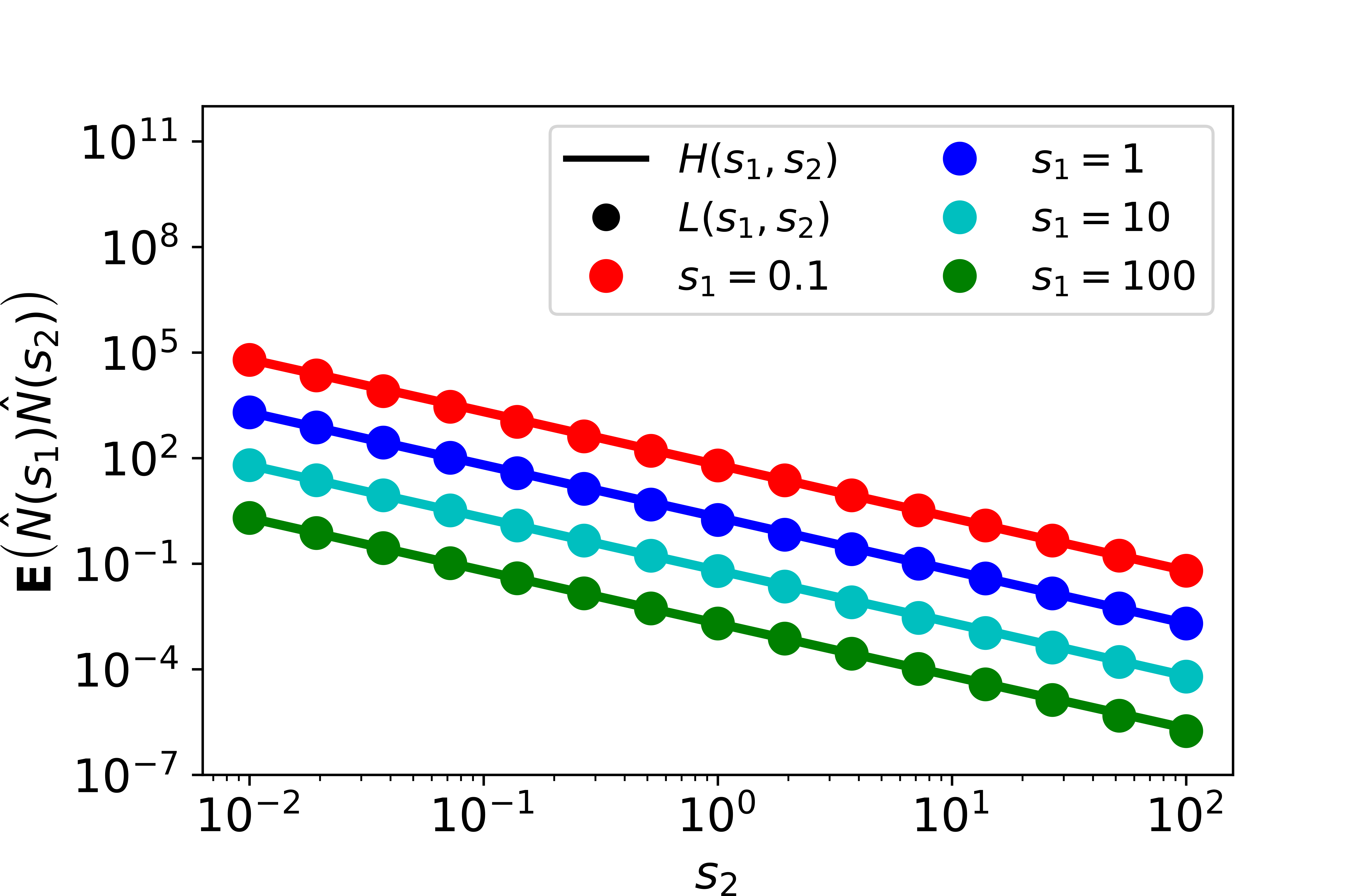
Here we show that the Laplace transform of the covariance of the span of a 1d Brownian motion obtained in Annesi et al. 2019 is retrieved in our formalism. We note the span process of the 1d Brownian motion ie the length of the visited domain at time as . We compare our result directly with the formula for the covariance as a function of time obtained in Annesi et al. 2019 (taking the diffusion coefficient ),
(28)
with
Figure S1: Comparison of the Laplace transform of the two point expectation, , obtained in Annesi et al. 2019 and the same quantity obtained using our formalism, Eq. (29).
We compare the result in Eq. (A.2) from Annesi et al. 2019 with the one obtained from our Eqs. (18) and (27) by splitting the integral into the domains , , and :
(29)
with
(30)
and
(31)
The numerically calculated functions and coincide as shown in Figure S1.
A.3 Derivation of Eq. (10) in the main text
We compute the difference between the distributions and in the limit and fixed for and , and . Starting from Eq. (25), we have
(32)
with
(33)
Appendix B -time span distributions
B.1 Derivation of Eq. (11) in the main text
For the probability distribution of the events , its multivariate Laplace transform is obtained by performing the same steps as those that led to (A.1),
(34)
The formula for the -time span distribution in the time domain is given similarly to (25) by recursively performing the inverse Laplace transforms, first on , then on , …until , (here supposing that ),
(35)
Similarly to Eq. (26), the case for any follows from Eq. (35).
Additionally, we obtain the expression for the -time span distribution for a Brownian motion with arbitrary diffusion constant by noting that the previous result pertains to the particular choice .
B.2 Derivation of Eq. (12) in the main text
We treat the limit ; i.e., . Starting from Eq. (34), with fixed, we have
(36)
Thus we obtain a result similar to the -time span distribution for the first-order correction to the product of independent one-time span distributions:
(37)
Consequently, with , and using the Tauberian theorem,
(38)
Here can be obtained either by Laplace inversion of the term of the sum, or starting directly from (35) and keeping the first order term in ,
(39)
being the span process of the Brownian motion of parameter as defined in Appendix A.2.
Appendix C Two-time trapping problem
Starting from Eq. (1) of the main text, and going to the continuum limit, we have
(40)
(41)
We now discuss the different regimes:
(a)
: In this limit, for , and is a decreasing exponential at large times (since this quantity is related to the exit probability from an interval). Thus,
(42)
where depends only on and but not on .
(b)
: From the scale invariance of Brownian motion, as the law of is the same as the one of , the term dominates. We note that corresponds to the probability of exiting an interval of unit size after a time , whose scaling behaviour is known to be , Eq. (5.219) of Weiss 1994. Thus,
(43)
(c)
: The term which dominates is still , as the integral in is decreasing (at least as a stretched exponential). Moreover, the conditional survival probability converges to a value that is neither 0 nor 1:
(44)
This limit is illustrated in Fig. 4 of the main text, as a function of .
Appendix D Run-and-tumble particle
D.1 Derivation of Eq. (13) in the main text
We consider the exit time distribution, , from the interval , for a run-and-tumble particle that starts at position with speed , respectively. This distribution obeys the following coupled differential equations
(45)
with and . Laplace transforming Eq. (45), we obtain the Laplace transform of the exit-time distribution from an interval of length when the walk starts at position :
(46)
where . Keeping only the first-order terms in the limit , we have
(47)
with
(48)
To obtain the exit time distribution in the time domain from (48) is difficult. However, in the diffusive limit ; i.e., and fixed, one can obtain simple results. By keeping the first order terms of in this limit, we get
(49)
Thus, with , and defining as the span process for a run and tumble particle and the span process for a Brownian motion,
(50)
Consequently, we have that
(51)
and differentiating this equation, we finally obtain
(52)
D.2 Comment on Eq. (13) in the main text
D.2.1 First-order correction to the covariance
We look at the -time span distribution in the limit and fixed. We do the asymptotic development up to the first relevant order
(53a)
(53b)
(53c)
(53d)
Integration of Eq. (53a) gives the product of the first moments. Eq. (53b) gives the same contribution to the covariance as the symmetric random walk. Integration of Eq. (53c) with respect to and leads to the first-order correction to the difference of the covariances. However, this integral vanishes. This means that one should compute the correction at the next order, using (53d). This leads to
(54)
D.2.2 First-order correction to the span distribution
We study the correction to the diffusive limit of the two-time span distribution in the limit ; i.e., . Keeping only the dominant terms, we have
(55)
If we focus on the behavior of this distribution for a typical realization; i.e., situations for which is fixed, with and , we have
(56)
This means that in the time domain the relative difference between the two cumulative distributions in the case where is fixed behaves as .
Appendix E Biased random walk
E.1 Derivation of Eq. (14) in the main text
First, we write the continuum limit exit-time distribution of the biased random walk of speed , see Eq. (2.2.28) of Redner 2001, when the walk starts at distance to the left boundary of the interval of size (and exits the interval either to the left or to the right side):
(57)
with . Here the superscripts refer to the left and right ends of the interval. Similarly, by reversing the direction of the velocity, we have
(58)
We use the convention , corresponding to starting with a single visited site at time 0, which is both on the left and right side of the interval of size 1. We define the indices direction (left, , or right, , end of the visited interval) of the random walker when the site is first visited. Performing the same calculation as in Appendix B we get
(59)
We use the transfer matrix technique by defining
(60)
In the limit (taking fixed), we obtain , with
(61)
Using this matrix notation, we have the simpler formula
where the vector is .
Performing the product of matrices having the same argument , we rewrite the previous equation as
(63)
where
(64)
and represents the -ordering operator. Eq. (64) is equivalent to the set of partial differential equations
with .
E.2 The one-time span distribution
The one-time span distribution derived in Wiese 2020 can be retrieved using Eq. (63). Consider the Laplace transform of the distribution of the number of distinct sites visited at a single time,
(65)
where is solution of with as follows from Eq. (64).
We solve the system of equations for (for the sake of simplicity, we drop the argument and write ):
(66)
Solving these coupled equations, we obtain
(67)
To obtain the distribution of the number of distinct sites visited in the time domain, we perform the inverse Laplace transform of , identifying the poles at and , :
(68)
(69)
(70)
By reversing the velocity, , we get the inverse Laplace transform of , namely, . We check numerically in Figure S2 that is indeed the same as the expression obtained in Wiese 2020.
Figure S2: Cumulative distribution of the span at times and for parameters and . The curves are , while the circles are from Wiese 2020.
E.3 Derivation of the -time span distribution
For the -time span distribution, we need the general expression of the matrices . We solve the set of partial differential equations (66) starting at to with arbitrary initial conditions .
Defining and , we have that
The expression for is similar and is obtained by reversing the velocity and the indices .
Thus we obtain, using (78), the exact expression of the matrix
(79)
with
(80)
(81)
and all the dependence being within the variable .
Hence, the knowledge of Eqs. (63), (79), (80), (81) give us the full description of the stochastic process , the span of a biased random walk.
Appendix F Illustration of Eq. (13) and (14)
Figure S3: -time distribution for the persistent random walk for parameters and (a), as well as for a biased random walk of parameters and diffusion , at times (b). Numerical simulations are represented by the dots.
We numerically invert the Laplace transform of the time distributions of a run-and-tumble particle using Eq. (13) and of a biased random walk using Eq. (14) of the main text. As shown in Figure S3, knowledge of the Laplace transformed distributions can be used to extract numerical values of the statistics, besides the theoretical characterization.
References
Vineyard (1963)G. H. Vineyard, J.
Math. Phys. 4, 1191
(1963).
Montroll and Weiss (1965)E. W. Montroll and G. H. Weiss, J.
Math. Phys. 6, 167
(1965).
Weiss (1994)G. Weiss, Aspects and Applications
of the Random Walk (Amsterdam, Netherlands:
North-Holland, 1994).
Hughes (1995)B. Hughes, Random Walks and Random
Environments (New York: Oxford University Press, 1995).
Feller (2008)W. Feller, An Introduction To
Probability Theory and its Applications (John
Wiley & Sons, 2008).
Rosenstock (1970)H. B. Rosenstock, J.
Math. Phys. 11, 487
(1970).
Donsker and Varadhan (1979)M. D. Donsker and S. Varadhan, Commun. Pure and Appl. Math. 32, 721 (1979).
Grassberger and Procaccia (1982)P. Grassberger and I. Procaccia, J.
Chem. Phys. 77, 6281
(1982).
Havlin et al. (1984)S. Havlin, M. Dishon,
J. E. Kiefer, and G. H. Weiss, Phys. Rev. Lett. 53, 407 (1984).
Klafter and Blumen (1985)J. Klafter and A. Blumen, Chem.
Phys. Lett. 119, 377
(1985).
Cattuto et al. (2009)C. Cattuto, A. Barrat,
A. Baldassarri, G. Schehr, and V. Loreto, Proc. Natl. Acad. Sci. (USA) 106, 10511 (2009).
Yeung and Saad (2013)C. H. Yeung and D. Saad, J. Phys. A: Math.
Theor. 46, 103001
(2013).
Daniels and Smithies (1941)H. E. Daniels and F. Smithies, in Mathematical
Proceedings of the Cambridge Philosophical Society, Vol. 37 (Cambridge University Press, 1941) pp. 244–251.