DeepPropNet - A Recursive Deep Propagator Neural Network for Learning Evolution PDE Operators
Abstract
In this paper, we propose a deep neural network approximation to the evolution operator for time dependent PDE systems over long time period by recursively using one single neural network propagator, in the form of POD-DeepONet with built-in causality feature, for a small time interval. The trained DeepPropNet of moderate size is shown to give accurate prediction of wave solutions over the whole time interval.
1 The Problem of Learning PDE Evolution Operator
Consider a second order evolution system
| (1) | ||||
| (2) |
where could be a scalar or vector. For a model problem, we will consider the inhomogeneous scalar wave (d’Alembert) equation
| (3) |
with the source term that is compactly supported on a bounded space-time domain where . This means that the source term differs from zero only on and operates for the limited time interval . When he solution to the Cauchy problem is given by:
| (4) |
The solution can be viewed through an evolution operator , which maps the initial conditions and the source term into the solution. Learning such a map between functions has been actively studied recently with various types of operator learning methods, including DeepONet [4] and Fourier Neural Operator [3]. The focus of this paper is to find an efficient way to learn this evolution operator with moderate size neural network for large time . For lack of a precise term, borrowing the term from quantum mechanics for the Green’s function propagator [5], we shall name the operator as the propagator for the evolution system. From (4), it is clear that if we like to train a neural network operator for large time t, the size of the network will grow for increasing time t. And, the amount of information to be input into a network will increase dramatically as t grows as well. We will propose a recursive propagator formulation for the evolution operator network.
First, the solution time interval will be divided into smaller subintervals
| (5) |
and for the solution is given by the propagator with initial condition of the solution and its velocity , i.e.,
| (6) |
where the initial condition would have been given by the propagator for the time block .
The propagators in (6) will be approximated by a single neural network in the form of DeepONet structure [2] with modification for time causality, namely,
| (7) |
Therefore, the propagator will be trained to map the initial and force function data into the solution . Moreover, this same propagator will be trained to approximate the solution for time periodic where the initial condition at can be computed with the propagator for the previous time interval . This procedure will be used recursively until we have trained the same propagator for the last time interval . Taken all together, we arrive at a propagator neural network for the whole time interval where the building block is the single propagator of moderate size . By controlling the size of the , the size of this propagator can be easily controlled for efficiency as well as accuracy. As the evolution PDE system has to observe the causality of the physical system, the DeepONet framework will be modified to include the causality, a previously proposed causality DeepONet in the study of dynamics system for modeling building response to seismic waves [4] will be used for this purpose.
The rest of the paper is organized as follows. In section 2, we will review the DeepONet [4] with time causality and extension with proper orthogonal decomposition (POD) approach for efficient treatment of spatial dependence of the solution. Section 3 will give the algorthmic outline of the DeepPropNet and numerical results of the DeepPropNet will be presented in Section 4. Finally, Section 5 gives a conclusion and some future work.
2 DeepONet with time causality and spatial POD
A causality DeepONet was proposed in [4] to handle the time casuality in dynamics system and was shown to be very effective to predict the seismic response of building. Here, we will just present the final form and for details please refer to [4].
Causality-DeepONet: A DNN representation of an operator for any continuous function with retarded response for is given as
| (8) |
where coefficents -all independent of continuous functions and .
To handle the spatial dependence of solution for the evolution system, we will adopt the idea of the POD-DeepONet[6, 7] which assumes there is a set of global basis for the targeted output which could be found by SVD, and the trunk net will be replaced by these basis, then the neural network is learning the mapping between values at sensors to the singular values if we consider using SVD as an example. Thus it may lose the ability to approximate arbitrary values of the operator in the computational domain given the values at sensors. The philosophy of POD-DeepONet is to find a set of basis globally, thus compress the memory and computation needed, which is the crux for learning the operator of the high dimensional problem.
Lu et al.[7] discussed the POD-DeepONets and proposed a time marching scheme for Fourier Neural Operator specifically to reduce the dimension of output, and they also proposed the modified DeepONet with feature expansion by feeding historical states of signal to trunk net as features. Bhattacharya et al.[6] proposed that they reduce the dimension of input and output by PCA and then learning the mapping between the reduced space by a neural network, and they also discussed the approximation quality needed to get good mappings. Meuris et al.[1] presented a procedure that learning the data-driven basis functions harnessing the DeepONet machinery and the learned basis function will be used by classical methods as custom basis to achieving high accurary for computation of arbitrary complex domain.
As for a problem with causality, The POD-DeepONet’s philosophy guides us either do the SVD for the whole outputs regardless the difference of temporal variables and spatial variables, or do specific SVD timestep by timestep to keep the causality for which we need to keep the basis for all time steps, or consider solution at each time step for each case as an independent target and find a common basis w.r.t spatial dimensions for all time steps & all cases. These ideas either burns the high memory cost, or destroy the causality in a brutal-force way. Therefore, a modification of POD-DeepONet for problem with causality is crucial. We follow the idea of POD-DeepONet but only construct the basis of spatial domain explicitly and utilize the causality DeepOnet to handle the temporal-dependent coefficients of each spatial basis.
In the following, we consider the 1d wave equation (3 and assume the right hand side has form
| (9) |
and the solution has a similar form
| (10) |
Next, we modify the Causality-DeepONet by
| (11) |
where is the elementwise multiplication, is the inner product,
| (12) | ||||
| (13) | ||||
| (14) | ||||
The activation functions of and are ReLU. Note the modes number in the CPOD-DeepONet(Causality POD-DeepONet) need to be greater than or equal to the number of given modes of right hand side in equation . The algorithm of the CPOD-DeepONet is shown in algorithm 1. To contain the memory efficiency and following the fact that equation has separation of variables, we will do outer product rather than computing point by points as shown in the last line of algorithm. This is one of the crux to handle higher dimensional problem.
Loss function Given batch size for training process and the total number of the test records , the loss function is defined as
| (15) |
where is the number of time step and is the number of points on direction.
To evaluate the training process, the mean of the relative L2 error is considered
| (16) |
The relative L2 error in a complete epoch is defined as
| (17) |
where is the number of batches, means the parameters of neural network at -th batch.
Similarly, we define the relative L2 error for the testing dataset
| (18) |
Note the is the total number of test cases.
Numerical Performance of Causality DeepONet with POD
Case 1: Constant wave-speed case In this test, we assume the wave speed is , and the right hand side satisfies
| (19) |
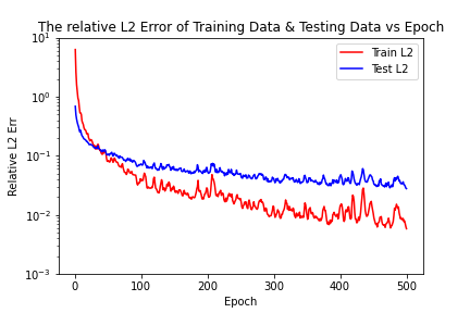
where are randomly sampled from . The exact solutions are from integrating the formula based on Duhamel’s method. There are 21 basis based on 19, thus, the input size of the causality DeepONet should be , where is the number of time steps. We set for all other cases in this paper. We build the branch part and trunk part of the causality DeepONet as -layer neural network with hidden neurons each layer and -layer neural network with hidden neurons each layer respectively, both of whose outputs dimension is and shrinking to dimension by inner product with the -basis. The learning rates during training including the following cases are . The batch size we choose for all the testing case is 20. The results trained 500 epochs with 1000 cases are shown in Figure 1.

Case 2: Variable wave-speed case
In this case we consider the case the wave speed is a function of
| (20) |
and the exact solution is given by
| (21) |
thus, the corresponding right hand side for (3) will be
| (22) | ||||
The inputs for the CPOD-DeepONet are the coefficients of basis funciton of in , since there are basis, the input size of the causality DeepONet should be . The causality DeepONet is as the same shape as in Case 1 but with different input dimensions. In this case we assume and with 400 equal spaced time steps, and there are 400 random sampled points on x-direction for each time step. We have similar results as shown in Figure 2. It should be mentioned that the trained CPOD-DeepONet can in fact be used to predict solution outside the trained spatial domains as shown in Fig. 3.


3 A Recursive DeepPropNet for Learning Evolution PDE Operators
Following the semi-group formulation of evolution PDEs, the DeepPropNet computes block by block along the time direction recursively. The initial conditions for the PDEs will be included together with the force functions for the time block as an input for DeepPropNet to assure the well-posedness of the problem. And, the DeepPropNet is then constructed recursively with a Causality DeepONet with POD to learn the PDE evolution operator over long time interval.
To simplify notation, we denote the initial conditions on the solution and its velocity as
| (23) |
and the DeepPropNet . Following the notations of Causality DeepONet with POD in equation , we define the DeepPropNet as
| (24) |
where is the branch net , is the corresponding trunk net as shown in equation . Likewise, are the trunk net and branch net of the vanilla DeepONet,
| (25) |
the corresponding -th output of trunk net is
| (26) |
The notation is abused to some extent in above equations, but the ’s and ’s on the right hand side means different neural networks. The definition of is as the same as . Note the summation of and in the equation is inspired from the superposition of linear waves from different sources and other format could be explored for nonlinear problems.
Recursive Formulation of DeepPropNet: To predict the wave field in the time block at beginning, the Deep Propagator DeepPropNet is to learn the mapping
| (27) |
Once the Deep Propagator is learned, the wave field in the next time block could be predicted by the Deep Propagator by using the initial propagator as follows
| (28) |
where the initial condition is replaced by the prediction of DeepPropNet at time .
The resulting propagator for the time block then will be again to be used to provide the initial condition for and the same initial propagator network for the time period . This procedure can be carried on recursively until the whole time period is covered,a global propagator network is thus obtained. Since it is like the initial propagator solver tracks the waves and propagates with the solutions along time direction and the propagator itself is a deep neural network, we call it Deep Propagator.
The schematics of the Deep Propagator DeepPropNet are shown in Algorithm 2. This is another crux to solve high dimensional problem. As illustrated in section 1, the input size could explode since the global dependence of source term, by solving it block by block recursively combining with the memory-efficient trick from separation of variables, learning high dimensional evolutioin operators is manageable now.
Loss function Similar to the loss function in section 2, we will define the loss function of DeepPropNet block by block in time. Given a batch size for training process, number of blocks and the total number of the test records , the loss function is defined as
| (29) |
where the -th block starts from but ends in and is the number of points on direction.
Likewise, the mean of the relative L2 error is considered as the relatvie L2 error in the total time-spatial domain
| (30) |
where is the i-th block of time and spatial domain.
4 Numerical Results of DeepPropNet
The equation and right hand sides are as the same as the non-constant wave speed case , but we split 5 equal sized blocks in time domain and for each block, there are 80 sampled time locations for training. The causality DeepONet is as the same shape as in Case 2 but with different input dimensions since the dependence of time steps shrinks. The vanilla DeepONet is a composition of a -layer fully connected neural network with hidden neurons each layer as branch net and a -layer fully connected neural network with hidden neurons each layer as trunk net, both of whose output dimensions are also . The initial data for each block will be given by true data. Figure 5 shows the prediction of the exact solution up to time with a maximum relative error of .
Training with DeepPropNet Prediction as Initial Condition at . There are two strategy to provide initial conditions for each block, either provide the exact solution or the prediction . We compare the relative L2 error evolution of these different process and as shown in Figure 6, they have similar loss convergence. The results are shown in Figure 4 and Figure 5 respectively. This is a natural test about the capability of the interpolation in training domain of the neural network, but it offers a convenience that there is no further need to prepare exact data on grids for initial conditions of each time blocks.



5 Conclusion and Future works
In this paper, we proposed the recursive way to construct DeepPropNet - a DNN propagator for evolution system over large time period by using a single building block propagator over a small time period, thus reducing the overall complexity and size of the neural network required. For the design of the DeepPropNet, we also extended the Causality DeepONet with POD with specific basis to alleviate the memory burden for large spatial variables. By seperately handling the spacial and temporal domain, we gain not only the memory efficiency but also the training boost. The preliminary numerical results have shown the feasibility of this recursive DeepPropNet in predicting the time evolution of wave propagations.
The proposed DeepPropNet here is based on a supervised learning approach where the data can be generated by a separate numerical methods or observation data or analytical solution when available. In theory, we could also use a unsupervised learning procedure to train the DeepPropNet by using the following residue of the PDEs as the loss function.
| (31) |
It is also natural to extend this framework to learn high frequency problem, since the spatial oscillating terms will be handled explicitly by the basis, but the temporal oscillating terms could be handled by the Causality DeepONet, based on our experience in the work [4].
Future work will be conducted on more complex evolution systems, the unsupervised training, training over partial time domain, highly oscillating problems and higher dimensional problems as well as initial boundary value problems.
References
- [1] Brek Meuris, Saad Qadeer, and Panos Stinis. Machine-learning custom-made basis functions for partial differential equations. arXiv:2111.05307 [cs, math], November 2021.
- [2] Lu L, Jin P, Pang G, Zhang Z, Karniadakis GE. Learning nonlinear operators via DeepONet based on the universal approximation theorem of operators. Nature Machine Intelligence. 2021 Mar;3(3):218-29.
- [3] Li Z, Kovachki NB, Azizzadenesheli K, Bhattacharya K, Stuart A, Anandkumar A. Fourier Neural Operator for Parametric Partial Differential Equations. International Conference on Learning Representations 2020 Sep 28.
- [4] L.Z. Liu, K. Nath, W, Cai, Causality DeepONet for Nonlinear Operators for Building Seismic Wave Responses, manuscript, December, 2021.
- [5] R. Shankar, Principles of Quantum Mechanics, Kluwer Academic/Plenum Publisher,1994.
- [6] Kaushik Bhattacharya, Bamdad Hosseini, Nikola B. Kovachki, and Andrew M. Stuart. Model Reduction And Neural Networks For Parametric PDEs. The SMAI journal of computational mathematics, 7:121–157, July 2021.
- [7] Lu Lu, Xuhui Meng, Shengze Cai, Zhiping Mao, Somdatta Goswami, Zhongqiang Zhang, and George Em Karniadakis. A comprehensive and fair comparison of two neural operators (with practical extensions) based on FAIR data. arXiv:2111.05512 [physics], November 2021.