Entanglement detection with imprecise measurements

Introduction.— Deciding whether an initially unknown state is entangled is one of the central challenges of quantum information science Gühne and Tóth 2009; Horodecki et al. 2009; Friis et al. 2019. The most common approach is the method of entanglement witnesses, in which one hypothesises that the state is close to a known target and then finds suitable local measurements that can reveal its entanglement Horodecki et al. 1996; Terhal 2000; Lewenstein et al. 2000. In principle, this allows for the detection of every entangled state. However, it crucially requires the experimenter to flawlessly perform the stipulated quantum measurements. This is an idealisation to which one may only aspire: even for the simplest system of two qubits, small alignment errors can cause false positives Seevinck and Uffink 2007; Rosset et al. 2012. In contrast, by adopting a device-independent approach, any concerns about the modelling of the measurement devices can be dispelled. This entails viewing them as quantum black boxes and detecting entanglement through the violation of a Bell inequality Bancal et al. 2011; Moroder et al. 2013. However, Bell experiments are practically demanding Brunner et al. 2014. Also, many entangled states either cannot, or are not known to, violate any Bell inequality Werner 1989; Augusiak et al. 2014. In addition, for the common purpose of verifying that a non-malicious entanglement source operates as intended, a device-independent approach is to use a sledgehammer to crack a nut. In the interest of a compromise, entanglement detection has also been investigated in steering scenarios, in which some devices are assumed to be perfectly controlled and others are quantum black boxes Wiseman et al. 2007. Nevertheless, such asymmetry is often not present in non-malicious scenarios, and the approach still suffers from drawbacks similar to both the device-independent case, albeit it milder, and the standard, fully controlled, scenario. A much less explored compromise route is to only assume knowledge of the Hilbert space dimension Moroder and Gittsovich 2012; Tavakoli et al. 2018. This essentially adopts the view that the experimenter has no control over the relevant degrees of freedom. Such ideas have also been used to strengthen steering-based entanglement detection Moroder et al. 2016.

Here, we introduce an approach to entanglement detection that neither assumes flawless control of the measurements nor views them as mostly uncontrolled operations. The main idea is that an experimenter can quantitatively estimate the accuracy of their measurement devices and then base entanglement detection on this benchmark. Such knowledge naturally requires a fixed Hilbert space dimension: the experimenter knows the degrees of freedom on which they operate. To quantify the inaccuracy between the intended target measurement and the lab measurement, we use a simple fidelity-based notion that can handily be measured experimentally.

In what follows, we first establish the relevance of small inaccuracies by showcasing that the conclusions of well-known entanglement witnesses can be substantially compromised. We show that the magnitude of detrimental influence associated to a small inaccuracy does not have to decrease for higher-dimensional systems. This is important because higher-dimensional entangled systems are increasingly interesting for experiments Dada et al. 2011; Erhard et al. 2020; Ecker et al. 2019; Herrera Valencia et al. 2020; Hu et al. 2020 but typically cannot be controlled as precisely as qubits. Secondly, we develop entanglement criteria that explicitly take the degree of inaccuracy into account. For two-qubit scenarios, we provide this based on the simplest entanglement witness and the Clauser-Horne-Shimony-Holt (CHSH) quantity. For a pair of systems of any given local dimension, we show that such criteria can be analytically established as corrections to a simple family of standard entanglement witnesses. Finally, we present semidefinite programming (SDP) relaxations for bounding the set of quantum correlations under measurement inaccuracies. We use this both to estimate the potentially constructive influence of measurement inaccuracy on entanglement-based correlations and to systematically place upper bounds for separable states on linear witnesses.

Framework.— We consider sources of bipartite states $\rho=\rho_{\text{AB}}$ of local dimension $d$. The subsystems are measured individually with settings $x$ and $y$ respectively, producing outcomes $a,b\in\{1,\ldots,o\}$. The experimenter’s aim is to measure the first (second) system using a set of projective measurements $\{\tilde{A}_{a|x}\}$ ($\{\tilde{B}_{b|y}\}$). These are called target measurements. However, the measurements actually performed in the lab do not precisely correspond to the targeted measurements, but instead to positive operator-valued measures (POVMs) $\{A_{a|x}\}$ ($\{B_{b|y}\}$). These are called lab measurements and do not need to be projective. The correlations in the experiment are given by the Born-rule

We quantify the correspondence between each of the target measurements and the associated lab measurements through their average fidelity,

The fidelity respects $\mathcal{F}\in[0,1]$ with $\mathcal{F}=1$ if and only if the lab measurement is identical to the target measurement. Importantly, the fidelity admits a simple operational interpretation: it is the average probability of obtaining outcome $a$ ($b$) when the lab measurement is applied to each of the orthonormal states spanning the eigenspace of the $a$-th ($b$-th) target projector. Thus, the fidelities $\{\mathcal{F}^{\text{A}}_{x},\mathcal{F}^{\text{B}}_{y}\}$ can be directly determined by probing the lab measurements with single qudits from a well-calibrated, auxiliary, source. This requires no entanglement and can routinely be achieved, see e.g. Ref. Bouchard et al. 2018. It motivates the assumption of a bounded inaccuracy, i.e. a lower bound on each of the fidelities,

where the parameter $\varepsilon\in[0,1]$ is the inaccuracy of the considered lab measurement. In the extreme case of $\varepsilon=0$, the lab measurement is identical to the target measurement and our scenario reduces to a standard entanglement witness. In the other extreme, $\varepsilon=1$, only the Hilbert space dimension of the measurement is known. Away from these extremes, one encounters the more realistic scenario, in which the experimenter knows the degrees of freedom, but is only able to control them up to a limited accuracy.

The simplest tests of entanglement use the minimal number of outcomes ($o=2$). In such scenarios the fidelity constrains (3) can be simplified into

where we have defined observables $A_{x}\equiv A_{1|x}-A_{2|x}$ and $B_{y}\equiv B_{1|y}-B_{2|y}$. The observables can be arbitrary Hermitian operators whose extremal eigenvalue is bounded by unity, i.e. $\left\lVert A_{x}\right\rVert_{\infty}\leq 1$ and $\left\lVert B_{y}\right\rVert_{\infty}\leq 1$.

Notice that the proposed framework immediately extends also to multipartite scenarios.

Impact of inaccuracies in entanglement witnessing.— A crucial motivating question for our approach is whether, and to what extent, small inaccuracies in the measurement devices ($\varepsilon\ll 1$) impact the analysis of a conventional entanglement witness. We discuss this matter based on several well-known witnesses.

Firstly, consider the simplest entanglement witness for two qubits, involving two pairs local Pauli observables: $\mathcal{W}=\langle\sigma_{X}\otimes\sigma_{X}\rangle+\langle\sigma_{Z}\otimes\sigma_{Z}\rangle$. For separable states we have $\mathcal{W}\leq\mathcal{W}_{\text{sep}}=1$ and for entangled states $\mathcal{W}\leq\mathcal{W}_{\text{ent}}=2$. Consider now that the lab observables $\{A_{1},A_{2}\}$ and $\{B_{1},B_{2}\}$ only nearly correspond (4) to the target observables $\{\sigma_{X},\sigma_{Z}\}$. Since $\mathcal{W}_{\text{ent}}=2$ is algebraically maximal, it remains unchanged, but such is not the case for the separable bound $\mathcal{W}_{\text{sep}}$. Thanks to the simplicity of $\mathcal{W}$, we can precisely evaluate $\mathcal{W}_{\text{sep}}$ in the prevalent scenario when all measurement devices are equally inaccurate, i.e. $\varepsilon^{\text{A}}_{x}=\varepsilon^{\text{B}}_{y}=\varepsilon$. For a product state, we have $\mathcal{W}=\langle A_{1}\rangle\langle B_{1}\rangle+\langle A_{2}\rangle\langle B_{2}\rangle\leq\sqrt{\langle A_{1}\rangle^{2}+\langle A_{2}\rangle^{2}}\sqrt{\langle B_{1}\rangle^{2}+\langle B_{2}\rangle^{2}}$. Since the target measurements are identical on both sites and the factors are independent, they are optimally chosen equal. Then, it is easily shown that the optimal choice of Bloch vectors corresponds to aligning $A_{1}$ and $A_{2}$ ($B_{1}$ and $B_{2}$) to the extent allowed by $\varepsilon$. This leads to the following tight condition for entanglement detection (see Supplementary Material)

when $\varepsilon\leq\frac{1}{2}-\frac{1}{2\sqrt{2}}$ and $\mathcal{W}_{\text{sep}}=2$ otherwise. Importantly, the derivative diverges at $\varepsilon\rightarrow 0^{+}$. Hence, a small $\varepsilon$ induces a large perturbation in the ideal ($\varepsilon=0$) separable bound. In the vicinity of $\varepsilon=0$, it scales as $\mathcal{W}_{\text{sep}}\sim 1+4\sqrt{\varepsilon}$. For example, $\varepsilon=0.5\%$ leads to $\mathcal{W}_{\text{sep}}(\varepsilon)\approx 1.28$, which eliminates over a quarter of the range in which standard entanglement detection is possible, indicating the relevance of false positives.

Secondly, consider the CHSH quantity for entanglement detection, namely $\mathcal{W}=\langle\sigma_{X}\otimes\left(\sigma_{X}+\sigma_{Z}\right)\rangle+\langle\sigma_{Z}\otimes\left(\sigma_{X}-\sigma_{Z}\right)\rangle$. Here, we have targeted observables optimal for violating the CHSH Bell inequality Clauser et al. 1969. One has $\mathcal{W}_{\text{sep}}=\sqrt{2}$ and $\mathcal{W}_{\text{ent}}=2\sqrt{2}$. In contrast to the previous example, the fact that all correlations from $d$-dimensional separable states constitute a subset of all correlations based on local hidden variables implies that entanglement can be detected for any value of $\varepsilon$. However, as we show in Supplementary Material through an explicit separable model that we conjecture to be optimal, this fact does not qualitatively improve the robustness of idealised ($\varepsilon=0$) entanglement detection to small inaccuracies. We obtain

when $\varepsilon\leq\frac{1}{2}-\frac{1}{2\sqrt{2}}$ and $\mathcal{W}_{\text{sep}}=2$ otherwise. For small $\varepsilon$, we find $\mathcal{W}_{\text{sep}}\sim\sqrt{2}+4\sqrt{\varepsilon}$. An inaccuracy of $\varepsilon=0.5\%$ ensures $\mathcal{W}_{\text{sep}}\gtrsim 1.67$, which eliminates nearly a fifth of the range in which standard entanglement detection is possible.

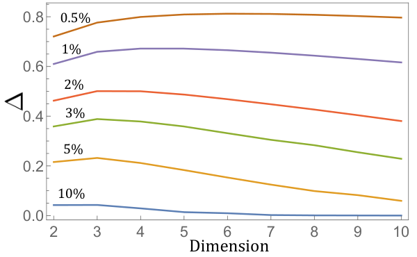
Interestingly, it is a priori not clear how small $\varepsilon$ should impact standard entanglement witnessing as $d$ increases. On the one hand, the impact ought to increase due to the increasing number of orthogonal directions in Hilbert space. On the other hand, it ought to decrease due to the growing distances in Hilbert space. For instance, the $\varepsilon$ required to transform the computational basis into its Fourier transform scales as $\varepsilon=\frac{\sqrt{d}-1}{\sqrt{d}}$, which rapidly approaches unity. To investigate the trade-off between these two effects, we consider the $d$-dimensional generalisation of the simplest entanglement witness. Both subsystems are subject to the same pair of target measurements, namely the computational basis $\{|e_{i}\rangle\}_{i=1}^{d}$ and its Fourier transform $\{|f_{i}\rangle\}_{i=1}^{d}$, where $|f_{i}\rangle=\Omega|e_{i}\rangle$ with $\Omega_{jk}=\frac{1}{\sqrt{d}}e^{\frac{2\pi i}{d}jk}$. The witness is $\mathcal{W}^{(d)}=\sum_{i=1}^{d}\langle e_{i},e_{i}|\rho|e_{i},e_{i}\rangle+\langle f_{i},f_{i}|\rho|f_{i},f_{i}\rangle$. Notice that for $d=2$ this only differs from the previous, simplest, witness by a normalisation term. One has $\mathcal{W}^{(d)}_{\text{sep}}=1+\frac{1}{d}$ and $\mathcal{W}^{(d)}_{\text{ent}}=2$ Spengler et al. 2012. Allowing for measurement inaccuracy, we use an alternating convex search algorithm to numerically optimise over the lab measurements and shared separable states to obtain lower bounds on $\mathcal{W}^{(d)}_{\text{sep}}(\varepsilon)$. See Supplementary Material for details about the method. In order to compare the impact of measurement inaccuracy for different dimensions, we consider the following ratio between the entangled-to-separable gap in the inaccurate and ideal case, $\Delta\equiv\frac{\mathcal{W}^{(d)}_{\text{ent}}(0)-\mathcal{W}^{(d)}_{\text{sep}}(\varepsilon)}{\mathcal{W}^{(d)}_{\text{ent}}(0)-\mathcal{W}^{(d)}_{\text{sep}}(0)}=\frac{d}{d-1}\left[2-\mathcal{W}^{(d)}_{\text{sep}}(\varepsilon)\right]$. Notice that the numerator features $\mathcal{W}^{(d)}_{\text{ent}}(0)$ instead of $\mathcal{W}^{(d)}_{\text{ent}}(\varepsilon)$ because $\varepsilon$ is not in itself a resource for the experimenter. The results of the numerics are illustrated in Figure 1 for some different choices of $\varepsilon$. We observe that $\Delta$ is not monotonic in $d$, but instead features a maximum, that shifts downwards in $d$ as $\varepsilon$ increases. Beyond this maximum point, the impact of measurement inaccuracies grows as the dimension becomes large.

Finally, for multipartite qubit states, it is natural to expect that the detrimental influence of small $\varepsilon$ grows with the number of qubits under consideration. The reason is that measurement inaccuracies can accumulate separately in the different subsystems. This intuition is confirmed by the models of Ref. Rosset et al. 2012, in which small alignment errors are used to spoof, with increasing magnitude, the standard fidelity-based witness of genuine multipartite entanglement for Greenberger-Horne-Zeilinger states Bourennane et al. 2004. This further confirms the need of considering measurement inaccuracies.

High-dimensional entanglement criterion.— In view of the the relevance of small measurement inaccuracies, it is natural to formulate entanglement criteria that take them explicitly into account beyond the simplest, two-qubit, scenario. Consider a pair of $d$-dimensional systems and $n\in\{1,\ldots,d^{2}-1\}$ measurements. For system A, the observables ideally correspond to (subsets of) a generalised Bloch basis $\{\lambda_{i}\}_{i=1}^{n}$ and for system B, the ideal observables are the complex conjugates $\{\bar{\lambda}_{i}\}_{i=1}^{n}$. Here, $\lambda_{i}$ is $d$-dimensional, traceless and satisfies $\Tr\left(\lambda_{i}\lambda_{j}^{\dagger}\right)=d\delta_{ij}$ Bertlmann and Krammer 2008. Defining $\rho=\frac{1}{d}\left(\openone+\sum_{i=1}^{d^{2}-1}\mu_{i}\lambda_{i}\right)$, one has $\left\lVert\vec{\mu}\right\rVert^{2}\leq d-1$. A simple standard entanglement witness, based on a total of $n$ measurements, is then given by

Using Hölder’s inequality, one finds that separable states obey $\mathcal{W}^{(d)}_{\text{sep}}=d-1$. When the choice of Bloch basis is fixed, entangled states can achieve at most $\mathcal{W}_{\text{ent}}^{(d)}=\nu_{\text{max}}\left[\sum_{i=1}^{n}\lambda_{i}\otimes\bar{\lambda}_{i}\right]$, by choosing the state as the eigenvector corresponding to the largest eigenvalue ($\nu_{\text{max}}$). When the choice of Bloch basis is not fixed, a general upper bound for entanged states is $\mathcal{W}^{(d)}_{\text{ent}}\leq\min\left\{\sqrt{n\left(d^{2}-1\right)},n(d-1)\right\}$, as shown in Supplementary Material. Note that $n(d-1)$ only is relevant when $d=2$. Notice also that the maximally entangled state $|\phi^{+}_{d}\rangle=\frac{1}{\sqrt{d}}\sum_{i=0}^{d-1}|ii\rangle$ achieves $\mathcal{W}^{(d)}=n$ regardless of the choice of Bloch basis.

Consider now that the lab observables only nearly correspond to $\{\lambda_{i}\}$ and $\{\bar{\lambda}_{i}\}$ respectively. We write them as $A_{i}=q\lambda_{i}+\sqrt{1-q^{2}}\lambda_{i}^{\perp}$ and $B_{i}=q\bar{\lambda}_{i}+\sqrt{1-q^{2}}\bar{\lambda}_{i}^{\perp}$, where $q\in[-1,1]$ is related to the inaccuracy through $q=1-2\varepsilon$ and $\lambda_{i}^{\perp}$ and $\bar{\lambda}_{i}^{\perp}$ are observables orthogonal to $\lambda_{i}$ and $\bar{\lambda}_{i}$, respectively, on the generalised Bloch sphere. In Supplementary Material, we prove that the witness $\mathcal{W}^{(d)}=\sum_{i=1}^{n}\langle A_{i}\otimes B_{i}\rangle$ for separable states obeys

when $q\geq\frac{1}{\sqrt{n}}$ and otherwise $\mathcal{W}^{(d)}_{\text{sep}}(\varepsilon)\leq n\left(d-1\right)$, which is algebraically maximal. As is intuitive, the window for detecting entanglement shrinks as $\varepsilon$ increases.

We investigate the tightness of the bound. To this end, choose the state as $|\phi^{\dagger}\rangle\otimes|\phi^{T}\rangle$, where the local Bloch vector is $\mu_{i}=\frac{\sqrt{d-1}}{\sqrt{n}}$ and where $\lambda_{i}\rightarrow\lambda_{i}^{\dagger}$ ($\lambda_{i}\rightarrow\lambda_{i}^{T}$) for $|\phi^{\dagger}\rangle$ ($|\phi^{T}\rangle$). Choose the observables as $A_{i}=q\lambda_{i}+\sum_{j\neq i}\frac{\sqrt{1-q^{2}}}{\sqrt{n-1}}\lambda_{j}$ and $B_{i}=q\bar{\lambda}_{i}+\sum_{j\neq i}\frac{\sqrt{1-q^{2}}}{\sqrt{n-1}}\bar{\lambda}_{j}$. This returns the separable bound (8). However, we need to check that the Bloch vector $\vec{\mu}$ corresponds to a valid state. Curiously, for the most powerful case, namely $n=d^{2}-1$, tightness would be implied by a positive answer to the long-standing open question of whether there exists a Weyl-Heisenberg covariant symmetric informationally complete (SIC) POVM in dimension $d$. To see the connection, simply choose the Bloch basis as the non-Hermitian Weyl-Heisenberg basis $\{X^{u}Z^{v}\}$ for $u,v\in\{0,\ldots,d-1\}$ and $u+v>0$, where $X=\sum_{k=0}^{d-1}|k+1\rangle\langle k|$ and $Z=\sum_{k=0}^{d-1}e^{\frac{2\pi ik}{d}}|k\rangle\langle k|$. It follows immediately that $|\langle\phi|X^{u}Z^{v}|\phi\rangle|=\frac{1}{\sqrt{d+1}}$, which defines a SIC-POVM. Since these SIC-POVMs are conjectured to exist in all dimensions Zauner 2011, and are known to exist up to well above the first hundred dimensions Scott 2017; Fuchs et al. 2017, our bound is plausibly tight for any $d$.

SDP methods.— We develop a hierarchy of SDP relaxations to bound the largest possible value of any linear witness, $\mathcal{W}=\sum_{a,b,x,y}c_{abxy}p(a,b|x,y)$, for some real coefficients $c_{abxy}$. The method applies both for correlations originating from entangled states and from separable states, under any given degree of measurement inaccuracy and arbitrary target measurements. Thus, we systematically establish upper bounds $\mathcal{W}^{\uparrow}_{\text{ent}}(\varepsilon)\geq\mathcal{W}_{\text{ent}}(\varepsilon)$ and $\mathcal{W}^{\uparrow}_{\text{sep}}(\varepsilon)\geq\mathcal{W}_{\text{sep}}(\varepsilon)$. This has a three-fold motivation. Firstly, $\mathcal{W}_{\text{ent}}$ will generally depend on $\varepsilon$; cases with $\mathcal{W}^{(d)}>\mathcal{W}^{(d)}_{\text{ent}}(0)$ can be observed when the inaccuracies accumulate in a constructive way (e.g. a favourable systematic error in the local reference frames). It is relevant to bound such occurances. Secondly, knowledge of $\mathcal{W}^{\uparrow}_{\text{ent}}(\varepsilon)$ allows an experimenter to give lower bounds on the inaccuracy of the measurement devices. Thirdly, and most importantly, this enables a general and systematic construction of entanglement witnesses of the form $\mathcal{W}\leq\mathcal{W}^{\uparrow}_{\text{sep}}(\varepsilon)$.

We discuss the main features of the method for computing $\mathcal{W}_{\text{ent}}^{\uparrow}(\varepsilon)$ and then see how it can be extended to also compute $\mathcal{W}_{\text{sep}}^{\uparrow}(\varepsilon)$. To this end, as is standard, the SDP relaxation method is based on the positivity of a moment matrix. This matrix consists of traces of monomials (in the spirit of e.g. Burgdorf and Klep 2012) which are composed of products of the state, the lab measurements and the target measurements (see Supplementary Material for specifics). Moments corresponding to products of the first two can be used to build a generic linear witness $\mathcal{W}$ via Eq. (1). Moments corresponding to products of the final two can be used to build the constraints on the fidelities $\mathcal{F}^{\text{A}}_{x}$ and $\mathcal{F}^{\text{B}}_{y}$. Our construction draws inspiration from two established ideas. Firstly, one can capture the constraints of $d$-dimensional Hilbert space, on the level of the moment matrix, by numerically sampling states and measurements Navascués and Vértesi 2015. Secondly, in scenarios without entanglement, constraints capturing the fidelity of a quantum state with a target can be incorporated into the moment matrix Tavakoli 2021. We adapt the latter to entanglement-based scenarios and measurement fidelities as needed for Eq. (3). Details are given in Supplementary Material. We have applied this method, at low relaxation level, in several different case studies in low dimensions and frequently found that the obtained upper bounds coincide with those obtained from interior point optimisation routines. We note that the computational requirements for this tool can be much reduced since sampling-based symmetrisation methods of Ref. Tavakoli et al. 2019 can straightforwardly be incorporated.

To extend this method for the computation of $\mathcal{W}_{\text{sep}}^{\uparrow}(\varepsilon)$, we must incorporate constraints on the set of quantum states. Since the set of separable states is generally difficult to characterise (see e.g. Doherty et al. 2002), we instead adopt an approach in which we use the ideal entanglement witness condition, $\mathcal{W}\leq\mathcal{W}_{\text{sep}}(0)$, which we may realistically assume to possess, in place of the set of separable states. Then, since the probabilities associated to performing the target measurements on the state explicitly appear in our moment matrix, we can introduce it as an additional linear constraint in our SDP. Hence, the optimisation is effectively a relaxation of the subset of entangled states for which the original entanglement witness holds. In fact, since the set of separable states is characterised by infinitely many linear entanglement witnesses, one can in this way continue to introduce linear standard witnesses to constrain the effective state space in the SDP and thus further improve the accuracy of the bound $\mathcal{W}_{\text{sep}}^{\uparrow}(\varepsilon)$. In Supplementary Material we exemplify the use of this method, in its basic version, using only a single witness constraint $\mathcal{W}\leq\mathcal{W}_{\text{sep}}(0)$ on the state space, and show that it returns non-trivial, albeit not tight, bounds for two simple entanglement witnesses for relevant values of $\varepsilon$.

Discussion.— We have introduced and investigated entanglement detection when the measurements only nearly correspond to those intended to be performed in the laboratory. We have shown the relevance of the concept, presented explicit entanglement witnesses that take measurement inaccuracy into account, and finally shown how SDP methods can be applied to these types of problems. These results are a step towards a theoretical framework for detecting entanglement based on devices that are quantitatively benchmarked in an operationally meaningful and experimentally accessible manner.

Our work leaves several natural open problems. If given an arbitrary standard entanglement witness, how can we compute corrections due to the introduction of measurement inaccuracies? Our SDP method is a first step towards addressing this problem but better methods are necessary both in terms of computational cost and in terms of the accuracy of the separable bound. Moreover, for a given $d$, what is the smallest number of auxiliary global measurement settings needed to eliminate the diverging derivative for optimal standard entanglement witnesses under small measurement inaccuracy? In addition, can one extend our entanglement witnesses to witnesses of genuine higher-dimensional entanglement, e.g. by detecting the Schmidt number? Also, in this first work, we have focused on bipartite entanglement. It would be interesting to identify useful entanglement witnesses for multipartite states at bounded measurement inaccuracy. Finally, the framework proposed here for entanglement detection draws inspiration from ideas proposed in semi-device-independent quantum communications. Given that several frameworks for semi-device-independence recently have been proposed Van Himbeeck et al. 2017; Tavakoli et al. 2020; Tavakoli et al. 2022; Wang et al. 2019; Tavakoli 2021, there may be other similarly inspired avenues for entanglement detection based on quantitative benchmarks.