Quickest Change Detection in Anonymous Heterogeneous Sensor Networks

The problem studied in this paper is closely related to the problem of QCD under the multiple-channel setup [10, 11, 12, 13, 14, 15, 18, 19, 20, 21, 22, 23], where samples are collected from multiple sensors sequentially, and the goal is to detect a change in the data-generating distribution of some unknown subset of the sensors or all the sensors. These works assume that the sensors are non-anonymous, i.e., it is known that which sensor that each sample comes from. In the non-anonymous setting, algorithms can be designed by combining the CuSum statistics each calculated for one sensor. These algorithms inherit the nice property of the CuSum algorithm [39] which can be updated in an online and recursive fashion, and thus is computationally efficient. It was shown in these studies that such a type of algorithms are asymptotically optimal for various scenarios. In this paper, we are interested in the anonymous setting, where at each time step the fusion center receives $n$ arbitrarily permuted (unordered) observations, and the permutations at different time steps may be different due to anonymity. Then, the fusion center does not know which samples over time come from one particular sensor. Therefore, existing approaches based on the idea of combining local CuSum statistics are not applicable any more since the fusion center is not able to compute one CuSum statistic for each node.

In anonymous networks, the fusion center does not know the exact distribution of each sample due to the uncertainty caused by the anonymity [2]. The group label that assigns the samples to different types of sensors is an unknown parameter of the distribution. Therefore, the QCD problem in anonymous networks can be viewed as a composite QCD problem with unknown pre- and post-change distributions [40, 41, 42, 43, 44, 45, 46], The main difference lies in that the unknown parameter in our problem is changing with time, i.e., the group label may not be the same at different time steps, and thus the samples are not identically distributed in the pre- or post-change regime. As will be shown in our numerical results, a generalized likelihood ratio based test does not work well here. Furthermore, we do not assume that the distributions belong to any parameterized family of distributions, e.g., exponential family.

The problem of quickest detection of a moving anomaly was studied in [47, 48], where an unknown sensor is affected by an anomaly with an unknown trajectory that emerges in the network at some unknown time. In [47], the statistical behavior of the samples is modeled using a hidden Markov model [49], and the trajectory is modeled as a deterministic and unknown one in [48]. Our work is different from the one in [47] since we do not put any assumption on the prior of group label (trajectory of the anomaly in [47]). The study in [48] is related to ours in that the samples can be equivalently viewed as being collected from anonymous sensors since the node affected by the anomaly is unknown.

The offline hypothesis testing problem in the anonymous setting was investigated in [2], where one sample is collected from each sensor. A mixture likelihood ratio test (MLRT) was developed, and was further shown to be optimal under the Neyman-Pearson setting. Here, we consider the QCD problem under the anonymous setting with sequential samples and time-varying group labels. We are interested in the tradeoff between the false alarm rate and average detection delay, which requires construction of sequential tests and more involved optimality analysis.

In Table I, we summarize the difference between our paper and other related works. We note that the fusion center may be able to recover the group identity if it performs, e.g., hypothesis testing, and the error probability depends on the distance between the distributions of different groups. With unordered samples, perfect anonymity can only be guaranteed if distributions among different groups are exactly the same. Designing optimal mechanisms to achieve perfect anonymity is not the focus of this paper, and might be of independent interest. In this paper, we focus on the design of optimal quickest detection algorithms for the scenario with unordered samples.

We first revisit the non-sequential hypothesis testing problem with anonymous heterogeneous sensors. We provide a simple proof for the optimality of the MLRT [2]. The basic idea is to construct a binary composite hypothesis testing problem with uniform priors on all possible group labels, and to show that the optimal test for the case with a uniform Bayesian prior is also optimal under the minimax setting.

For the QCD problem in anonymous networks, we design a mixture CuSum algorithm, and prove that the mixture CuSum algorithm is exactly optimal under Lorden’s criterion [50]. To show its exact optimality, we build a novel connection among several simple QCD problems and the QCD problem under the anonymous setting. The major challenge in our analysis is due to that we are optimizing the worst-case performance over all possible change-point, group labels and pre-change observations.

The computational complexity of the mixture CuSum algorithm at each time step increases almost exponentially in the number of nodes, and thus is not efficient when the network is large. We then propose a computationally efficient test based on the asymptotic behavior of the mixture CuSum test statistic when the network is large. The basic idea is to approximate the mixture CuSum statistic by a convex optimization problem with linear constraints, the computational complexity of which is independent of the number of sensors. We provide a comprehensive discussion of its performance. We also derive a lower bound on its worst-case average run length to false alarm, so that a threshold can be chosen analytically for false alarm control in practice.

We provide numerical results to demonstrate the performance of our proposed algorithms. We compare our algorithms with two other heuristic algorithms based on the Bayesian approach and the generalized likelihood ratio approach, and show that our mixture CuSum has the best performance, and our computationally efficient test also performs better than the other two tests. We also compare their computational complexity, and show that our the computationally efficient algorithm is much more efficient for large networks.

In Section II, we present the problem formulation. In Section III, we revisit the binary hypothesis testing problem in the anonymous setting, and derive a simple optimality proof for the MLRT. In Section IV, we develop the mixture CuSum algorithm, and prove its exact optimality under Lorden’s criterion. We further develop a computationally efficient test and characterize its performance theoretically. In Section V, we provide numerical results to validate our theoretical assertions. In Section VI, we present some concluding remarks.

We first revisit the binary hypothesis testing problem in [2]. The goal is to distinguish between the two hypotheses: $\mathcal{H}_{0}:\theta=0$ and $\mathcal{H}_{1}:\theta=1$.

Denote by $X^{n}=\{X_{1},\ldots,X_{n}\}$ the $n$ collected samples. Denote by $\sigma(i)\in\{1,\ldots,K\}$ the label of the group that $X_{i}$ comes from, i.e., $X_{i}\sim p_{\theta,\sigma(i)}$. Due to the anonymity, $\sigma(i)$, $i=1,\ldots,n$, are unknown to the fusion center. There are $\left(\begin{subarray}{c}n\\ n_{1},\ldots,n_{K}\end{subarray}\right)$ possible $\sigma:\{1,\ldots,n\}\rightarrow\{1,\ldots,K\}$ satisfying $|\{i:\sigma(i)=k\}|=n_{k},\forall k=1,\ldots,K.$ We denote the collection of all such labels by $\mathcal{S}_{n,\mathbf{\lambda}}$, where $\mathbf{\lambda}=\{n_{1},\ldots,n_{K}\}$.

Given $\sigma$, the $n$ collected samples are assumed to be independent. The problem is a composite hypothesis testing problem, where $\sigma$ is the unknown parameter for both $\theta=0$ and $1$:

The worst-case type-I and type-II error probabilities for a decision rule $\phi$ are defined as

where $\mathbb{E}_{{\theta,\sigma}}$ denotes the expectation under $\mathbb{P}_{{\theta,\sigma}}$, for $\theta\in\{0,1\}$ and $\sigma\in\mathcal{S}_{n,\mathbf{\lambda}}$. The Neyman-Pearson setting is studied, where the goal is to solve the following problem for any $\zeta\in[0,1]$:

In the QCD setting, anonymized samples are observed sequentially. At some unknown time $\nu$, an event occurs in the network, and changes the data-generating distributions of the sensors. Specifically, denote the $i$-th sample at time $t$ by $X^{n}_{i}[t]$ and all the observed samples at time $t$ by $X^{n}[t]$. Before the change, i.e., $t<\nu$, $X^{n}[t]\sim\mathbb{P}_{0,\sigma_{t}},\text{ for some {unknown} }\sigma_{t}\in\mathcal{S}_{n,\mathbf{\lambda}}.$ After the change, i.e., $t\geq\nu$, $X^{n}[t]\sim\mathbb{P}_{1,\sigma_{t}},\text{ for some {unknown} }\sigma_{t}\in\mathcal{S}_{n,\mathbf{\lambda}}.$ We note that $\sigma_{t}$ may change with time, i.e., $\sigma_{t_{1}}$ may not be the same as $\sigma_{t_{2}}$, for $t_{1}\neq t_{2}$. We assume that for any $t\geq 0$, given $\sigma_{t}$, the samples in $X^{n}[t]$ are independent. We further assume that $X^{n}[{t_{1}}]$ is independent from $X^{n}[{t_{2}}]$ for any $t_{1}\neq t_{2}$.

The objective is to detect the change at time $\nu$ as quickly as possible subject to false alarm constraints. In this paper, we consider a deterministic unknown change point $\nu$. We define the worst-case average detection delay (WADD) under Lorden’s criterion [50] and worst-case average run length (WARL) for any stopping time $\tau$ as follows:

where $\Omega=\{\sigma_{1},\sigma_{2},...,\sigma_{\infty}\}$, $\mathbb{E}^{\nu}_{\Omega}$ denotes the expectation when the change is at $\nu$, and the observations at time $t$ are labeled according to $\sigma_{t}$, and $\mathbf{X}^{n}[1,\nu-1]=\{X^{n}[1],\ldots,X^{n}[\nu-1]\}$.

The goal is to design a stopping rule that minimizes the WADD subject to a constraint on the WARL:

In this section, we list the notations used in this paper.

• •

  $n$ denotes the number of sensors, $K$ denotes the number of groups and $n_{k}$ denotes the number of sensor in group $k$.

• •

  $\bm{\alpha}=[\alpha_{1}\cdots\alpha_{K}]^{T}$, where $\alpha_{k}=\lim_{n\rightarrow\infty}\frac{n_{k}}{n}$ denotes the asymptotic fraction of sensors of group $k$.

• •

  $\sigma(i)\in\{1,\ldots,K\}$ denotes the label of the group that $X_{i}$ comes from, i.e., $X_{i}\sim p_{\theta,\sigma(i)}$, and $\mathcal{S}_{n,\mathbf{\lambda}}$ denotes the collection of all $\sigma(i)$, where $\mathbf{\lambda}=\{n_{1},\ldots,n_{K}\}$.

• •

  $H(\bm{\alpha})$ denotes the entropy of $\bm{\alpha}$.

• •

  $\Pi_{X^{n}}$ denotes the empirical distribution of samples $X^{n}$, and $T(\Pi_{X^{n}})$ denotes the type class of $\Pi_{X^{n}}$.

• •

  $\mathcal{P}_{n}$ denotes the set of types with denominator $n$.

• •

  $D(P\big|\big|Q)$ denotes the Kullback-Leibler (KL) divergence between $P$ and $Q$.

• •

  $f(x)\sim g(x)$ as $x\rightarrow x_{0}$ if $f(x)=g(x)(1+o(1))$ as $x\rightarrow x_{0}$.

Motivated by the fact that the MLRT is optimal for the binary composite hypothesis testing problem, we construct the following mixture CuSum algorithm:

Let $W[t]=\max\limits_{1\leq j\leq t}\sum_{i=j}^{t}\log\ell(X^{n}[i])$. The test statistic $W[t]$ has the following recursion:

The following theorem shows that the mixture CuSum algorithm is exactly optimal under Lorden’s criterion [50] in (6).

The missing details of the proof can be found in Appendix A and Appendix B. The asymptotic optimality under Pollak’s formulation [53] can also be derived similarly, and is ignored in this paper however due to space limitation.

The mixture likelihood ratio $\ell(X^{n}[i])$ needs to compute the average of the likelihood over all possible $\sigma\in{\mathcal{S}_{n,\mathbf{\lambda}}}$. Note that the size of ${\mathcal{S}_{n,\mathbf{\lambda}}}$ is $\binom{n}{n_{1},\cdots,n_{K}}$. From the exponential bounds on the size of a type class[54], we have that $\frac{2^{nH\big([\frac{n_{1}}{n}\cdots\frac{n_{K}}{n}]\big)}}{(n+1)^{\mid\mathcal{X}\mid}}\leq\binom{n}{n_{1},\cdots,n_{K}}\leq 2^{nH\big([\frac{n_{1}}{n}\cdots\frac{n_{K}}{n}]\big)},$ where $H\big([\frac{n_{1}}{n}\cdots\frac{n_{K}}{n}]\big)$ denotes the entropy of $[\frac{n_{1}}{n}\cdots\frac{n_{K}}{n}]$. As $n\rightarrow\infty$, we have that $\lim_{n\rightarrow\infty}H\big([\frac{n_{1}}{n}\cdots\frac{n_{K}}{n}]\big)=H(\bm{\alpha})$. Therefore, the computational complexity of mixture CuSum increases almost exponentially with $n$, which limits its practical applications in large networks. This motivates the need for computationally efficient tests for large networks. There are a wide range of applications in which the number of nodes is very large, e.g., IoT networks with thousands of sensors, smart grids with a large number of PMUs, crowdsourcing, and wireless sensor networks.

In this section, we focus on discrete distributions, that is, the cardinality of $\mathcal{X}$ is finite, where $\mathcal{X}$ denotes the alphabet of the distributions $p_{\theta,k},\forall\theta\in\{0,1\},k\in\{1,2,\cdots,K\}$. We note that our mixture CuSum algorithm and its exact optimality result apply to general distributions, which are not necessarily discrete. Denote by $\mathcal{P}_{\mathcal{X}}$ the set of all distributions supported on $\mathcal{X}$. We propose a computationally efficient algorithm and then derive a lower bound on its WARL so that a threshold can be chosen analytically for false alarm control.

We first introduce some useful results that motivate the design of our algorithm. Let $\Pi_{X^{n}}$ denote the empirical distribution of samples $X^{n}$, and let $T(\Pi_{X^{n}})$ denote the type class of $\Pi_{X^{n}}$. Then, it can be shown that ¹¹ 1 See Lemma 4.1 in [2] for the proof.

The right hand side of equation in (24) is a function of the empirical distribution $\Pi_{X^{n}}$. Let $\mathcal{P}_{n}$ denote the set of types with denominator $n$. For $n\geq 1$, let $Q_{n}\in\mathcal{P}_{n}$ be a sequence of distributions and $\lim_{n\rightarrow\infty}Q_{n}=Q$. The computation of the mixture likelihood ratio in (24) can be approximated by an optimization problem when $n$ is large using the fact ²² 2 See Lemma 5.2 in [2] for the proof. that

The right hand side of (IV-B) is a convex optimization problem with linear constraints, which can be solved efficiently using standard optimization tools [55, 56]. Its computational complexity is independent of the number of sensors. Therefore, for large $n$, the mixture over $\sigma$ in (24) can be approximated by solving a convex optimization problem whose computational complexity is independent of the network size $n$.

Let $\bm{P}=[P_{1}\cdots P_{K}]^{T}$, where $P_{k}\in\mathcal{P}_{\mathcal{X}}$, for $1\leq k\leq K$. For any $Q\in\mathcal{P}_{\mathcal{X}}$, define the following function of $Q$:

Intuitively, an algorithm for the problem in Section II can be constructed by approximating the log of the mixture likelihood ratio at time $t$ in the mixture CuSum algorithm using $n\big(f_{\bm{P}_{0}}(\bm{\alpha},\Pi_{\mathbf{X}^{n}[t]})-f_{\bm{P}_{1}}(\bm{\alpha},\Pi_{\mathbf{X}^{n}[t]})\big)$. However, the lower bound on the WARL for this algorithm is difficult to derive due to the “inf” in the test statistic. We construct a novel test that can be updated recursively, and for which a lower bound on WARL can be theoretically derived. Moreover, as will be numerically demonstrated, this test has a WADD-WARL trade-off that is close to the optimal mixture CuSum, while also being computationally efficient.

Let $\hat{\nu}_{t}$ denote the change point estimate at time $t$. Denote by $\hat{t}\triangleq t-\hat{v}_{t}+1$. We then design our detection statistic to approximate $W[t]$ in (18):

Instead of using a maximum likelihood approach to estimate $\hat{\nu}_{t}$ as in (18), which is not computationally efficient here, since $\hat{\nu}_{t}$ also appears in $\mathbf{X}^{n}[\hat{\nu}_{t},t]$, we design a recursive way of updating $\hat{\nu}_{t}$. Let $\hat{\nu}_{0}=0$. If $\widehat{W}[t]\leq 0$, $\hat{\nu}_{t+1}=t+1$, and if $\widehat{W}[t]>0$, $\hat{\nu}_{t+1}=\hat{\nu}_{t}$. Then, $\Pi_{\mathbf{X}^{n}[\hat{\nu}_{t},t]}$ can also be updated recursively: if $\widehat{W}[t]\leq 0$, $\Pi_{\mathbf{X}^{n}[\hat{\nu}_{t+1},t+1]}=\Pi_{\mathbf{X}^{n}[t+1]}$, and if $\widehat{W}[t]>0$, $\Pi_{\mathbf{X}^{n}[\hat{\nu}_{t+1},t+1]}=\frac{\hat{t}\Pi_{\mathbf{X}^{n}[\hat{\nu}_{t},t]}+\Pi_{\mathbf{X}^{n}[t+1]}}{\widehat{t}+1}$.

We next provide a heuristic explanation of how $\widehat{W}[t]$ evolves in the pre- and post-change regimes. According to the Glivenko–Cantelli theorem [57], before the change point $\nu$, as $n\rightarrow\infty$, $\Pi_{\mathbf{X}^{n}[\hat{\nu}_{t},t]}$ converges to $\bm{\alpha}^{T}\bm{P}_{0}$ almost surely. It can be easily seen that $f_{\bm{P}}(\bm{\alpha},Q)\geq 0$ for any $\bm{\alpha},\bm{P}$ and $Q$. The equality holds if and only if $\bm{\alpha}^{T}\bm{P}=Q$. This implies that $f_{\bm{P}_{0}}(\bm{\alpha},\bm{\alpha}^{T}\bm{P}_{0})-f_{\bm{P}_{1}}(\bm{\alpha},\bm{\alpha}^{T}\bm{P}_{0})<0$. Therefore, before the change point $\nu$, for large $n$, $\widehat{W}[t]$ has a negative drift. Similarly, after the change point $\nu$, for large $n$, $\widehat{W}[t]$ has a positive drift of $f_{\bm{P}_{0}}(\bm{\alpha},\bm{\alpha}^{T}\bm{P}_{1})$, and evolves towards $\infty$. This motivates us to construct the following computationally efficient test:

The computation cost of $\tau_{e}$ mainly lies in the update of the empirical distribution and the optimization step. The computational complexity of updating the empirical distribution increases linearly with $n$, and the computational complexity of the optimization step is independent of $n$. Therefore, the computationally efficient test is more efficient than the optimal mixture CuSum algorithm when $n$ is large. Table II summarizes the computational complexity of the mixture CuSum algorithm and the computationally efficient algorithm.

In the following theorem, we present a lower bound on the WARL for our computationally efficient test in (28).

In the following, we provide a proof sketch, and the full proof can be found in Appendix C.

To guarantee that $\inf_{\Omega}\mathbb{E}_{\Omega}^{\infty}\big[\tau_{e}(b)\big]\geq\gamma$, it suffices to choose $b$ such that $\frac{e^{b}}{\big(\frac{b}{h}+1\big)\big(\prod_{k}|\mathcal{P}_{\frac{b}{h}n_{k}}|\big)}=\gamma$ and $b\sim\log\gamma$.

Note that an upper bound on the WADD for $\tau_{e}$ is difficult to obtain. To understand the detection delay of the proposed computationally efficient test, we then study the case when the change occurs at $\nu=1$. We have the following result.

Intuitively, Proposition 1 implies that if the change is at $\nu=1$ and regeneration does not happen, then the detection delay of the computationally efficient algorithm increases linearly with the threshold $b$ at the rate of ${1}/(nf_{\bm{P}_{0}}(\bm{\alpha},\bm{\alpha}^{T}\bm{P}_{1}))$.

We then present the following universal lower bound on the WADD, and show that the slope is also ${1}/(nf_{\bm{P}_{0}}(\bm{\alpha},\bm{\alpha}^{T}\bm{P}_{1}))$ when $n$ is large.

By combining Propositions 1 and 2, it can be seen that the tradeoff between the WADD and WARL for our computationally efficient test is close to the optimal one when $n$ is large. This demonstrates the advantage of our test that for large networks, it has a similar statistical efficiency comparing to the optimal test, and has a significantly reduced computational complexity.

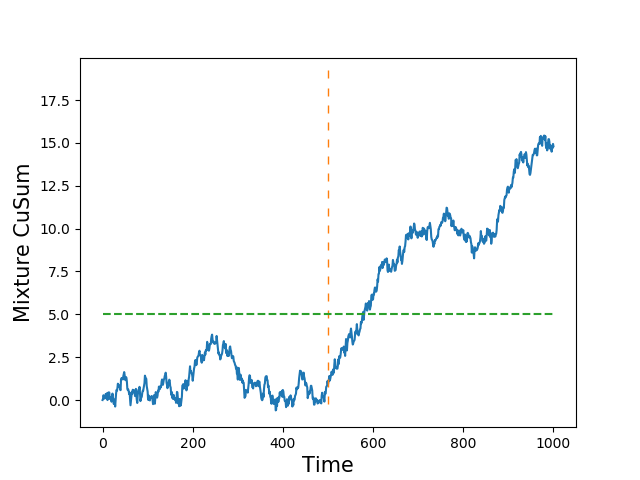
We first show an example evolution path of the mixture CuSum algorithm. Set $n=2$ and $K=2$, i.e., one sensor in each group. For group 1, the pre- and post-change distributions are $\mathcal{N}(0,1)$ and $\mathcal{N}(0.5,1)$, respectively. For group two, the pre- and post-change distribution are $\mathcal{N}(2,1)$ and $\mathcal{N}(1.5,1)$, respectively. In Fig. 10, we set the change point to be 500 and $b=5$. We plot one sample evolution path of the mixture CuSum algorithm. It can be seen that before the change point, the test statistic fluctuates around zero, and after the change point, it starts to increase with a positive drift.

We then compare our optimal mixture CuSum test with two other heuristic algorithms based on the Bayesian approach and the generalized likelihood ratio approach to tackling the unknown group assignments. For the Bayesian approach, we pretend that each sample comes from group $k$ with probability $n_{k}/n$, for $k=1,\ldots,K$, independently, so that on average the $k$-th group has $n_{k}$ sensors, although we actually have exact $n_{k}$ sensors in each group $k$. We then compute the following likelihood ratio:

The generalized likelihood ratio for the sample $x^{n}[t]$ is

We then design CuSum-type tests using (41) and (42), which are referred to as Bayesian and Generalized CuSums. The test statistics of these three algorithms are all symmetric, and therefore for different $\Omega$, the average detection delay and average run length are the same.

In Fig. 10, we plot the WADD as a function of the WARL. It can be seen that our mixture CuSum algorithm outperforms the other two algorithms. Moreover, the relationship between the WADD and log of the WARL is linear. The slope of these three curves should be the reciprocal of the expectation of the corresponding likelihood ratio under $\mathbb{P}_{1,\sigma}$ for some $\sigma\in{\mathcal{S}_{n,\mathbf{\lambda}}}$. Due to the fact that the distributions are continuous, our computationally efficient test is not applicable here.

For the computationally efficient algorithm, we first consider a simple example with $n=2$, $K=2$, $n_{1}=1$ and $n_{2}=1$. The pre- and post-change distributions for group 1 are binomial distribution $\mathcal{B}(10,0.5)$ and $\mathcal{B}(10,0.3)$, respectively, and for group 2 are $\mathcal{B}(10,0.5)$ and $\mathcal{B}(10,0.7)$, respectively. We plot a sample evolution path of the efficient algorithm in Fig. 10. Similar to the mixture CuSum, before the change point, the test statistic fluctuates around zero, and after the change point, it starts to increase with a positive drift.

We then compare the performance of our efficient algorithm with the optimal mixture CuSum algorithm, the Bayesian CuSum algorithm and the Generalized CuSum algorithm, and repeat the experiment for $n=8$, $n_{1}=4$, $n_{2}=4$ and $n=20$, $n_{1}=10,n_{2}=10$ with the same distributions.

References

- [1] Z. Sun, S. Zou, and Q. Li, “Quickest change detection in anonymous heterogeneous sensor networks,” in Proc. IEEE Int. Conf. Acoust. Speech Signal Process. (ICASSP), pp. 5925–5929, 2020.
- [2] W. N. Chen and I. H. Wang, “Anonymous heterogeneous distributed detection: Optimal decision rules, error exponents, and the price of anonymity,” IEEE Trans. Inform. Theory, vol. 65, no. 11, pp. 7390–7406, 2019.
- [3] V. V. Veeravalli and T. Banerjee, “Quickest change detection,” Academic press library in signal processing: Array and statistical signal processing, vol. 3, pp. 209–256, 2013.
- [4] A. Tartakovsky, I. Nikiforov, and M. Basseville, Sequential analysis: Hypothesis testing and changepoint detection. CRC Press, 2014.
- [5] H. V. Poor and O. Hadjiliadis, Quickest Detection. Cambridge University Press, 2009.
- [6] M. Basseville and I. V. Nikiforov, Detection of Abrupt Changes: Theory and Application. Prentice Hall, 1993.
- [7] D. O. Siegmund, Sequential Analysis: Tests and Confidence Intervals. Springer Series in Statistics, Springer, 1985.
- [8] A. G. Tartakovsky, Sequential Change Detection and Hypothesis Testing: General Non-iid Stochastic Models and Asymptotically Optimal Rules. CRC Press, 2019.
- [9] L. Xie, S. Zou, Y. Xie, and V. V. Veeravalli, “Sequential (quickest) change detection: Classical results and new directions,” IEEE Journal on Selected Areas in Information Theory, vol. 2, no. 2, pp. 494–514, 2021.
- [10] A. G. Tartakovsky and V. V. Veeravalli, “Change-point detection in multichannel and distributed systems,” Applied Sequential Methodologies: Real-World Examples with Data Analysis, vol. 173, pp. 339–370, 2004.
- [11] A. G. Tartakovsky, B. L. Rozovskii, R. B. Blazek, and H. Kim, “A novel approach to detection of intrusions in computer networks via adaptive sequential and batch-sequential change-point detection methods,” IEEE Trans. Signal Proc., vol. 54, no. 9, pp. 3372–3382, 2006.
- [12] Y. Mei, “Efficient scalable schemes for monitoring a large number of data streams,” Biometrika, vol. 97, no. 2, pp. 419–433, 2010.
- [13] Y. Xie and D. Siegmund, “Sequential multi-sensor change-point detection,” Ann. Statist., pp. 670–692, 2013.
- [14] G. Fellouris and G. Sokolov, “Second-order asymptotic optimality in multisensor sequential change detection,” IEEE Trans. Inform. Theory, vol. 62, no. 6, pp. 3662–3675, 2016.
- [15] V. Raghavan and V. V. Veeravalli, “Quickest change detection of a Markov process across a sensor array,” IEEE Trans. Inform. Theory, vol. 56, no. 4, pp. 1961–1981, 2010.
- [16] T. He, S. Ben-David, and L. Tong, “Nonparametric change detection and estimation in large-scale sensor networks,” IEEE Trans. Signal Proc., vol. 54, no. 4, pp. 1204–1217, 2006.
- [17] D. Ciuonzo and P. S. Rossi, “Dechade: Detecting slight changes with hard decisions in wireless sensor networks,” International Journal of General Systems, vol. 47, no. 5, pp. 535–548, 2018.
- [18] O. Hadjiliadis, H. Zhang, and H. V. Poor, “One shot schemes for decentralized quickest change detection,” IEEE Trans. Inform. Theory, vol. 55, no. 7, pp. 3346–3359, 2009.
- [19] M. Ludkovski, “Bayesian quickest detection in sensor arrays,” Sequential Analysis, vol. 31, no. 4, pp. 481–504, 2012.
- [20] S. Zou, V. V. Veeravalli, J. Li, and D. Towsley, “Quickest detection of dynamic events in networks,” IEEE Trans. Inform. Theory, vol. 66, no. 4, pp. 2280–2295, 2020.
- [21] V. V. Veeravalli, “Decentralized quickest change detection,” IEEE Trans. Inform. Theory, vol. 47, no. 4, pp. 1657–1665, 2001.
- [22] A. G. Tartakovsky and V. V. Veeravalli, “Asymptotically optimal quickest change detection in distributed sensor systems,” Sequential Analysis, vol. 27, no. 4, pp. 441–475, 2008.
- [23] S. Zou, V. V. Veeravalli, J. Li, D. Towsley, and A. Swami, “Distributed quickest detection of significant events in networks,” in Proc. IEEE Int. Conf. Acoust. Speech Signal Process. (ICASSP), pp. 8454–8458, 2019.
- [24] L. Atzori, A. Iera, and G. Morabito, “The internet of things: A survey,” Computer Networks, vol. 54, no. 15, pp. 2787–2805, 2010.
- [25] B. B. P. Rao, P. Saluia, N. Sharma, A. Mittal, and S. V. Sharma, “Cloud computing for internet of things amp; sensing based applications,” in 2012 Sixth International Conference on Sensing Technology (ICST), pp. 374–380, 2012.
- [26] S. Li, L. D. Xu, and X. Wang, “Compressed sensing signal and data acquisition in wireless sensor networks and internet of things,” IEEE Trans. Industr. Inform., vol. 9, no. 4, pp. 2177–2186, 2013.
- [27] A. Al-Fuqaha, M. Guizani, M. Mohammadi, M. Aledhari, and M. Ayyash, “Internet of things: A survey on enabling technologies, protocols, and applications,” IEEE Commun. Surv. Tutor., vol. 17, no. 4, pp. 2347–2376, 2015.
- [28] M.-C. Yuen, I. King, and K.-S. Leung, “A survey of crowdsourcing systems,” in IEEE International Conference on Privacy, Security, Risk and Trust and IEEE International Conference on Social Computing, pp. 766–773, 2011.
- [29] E. Estellés-Arolas and F. G.-L. de Guevara, “Towards an integrated crowdsourcing definition,” Journal of Information Science, vol. 38, no. 2, pp. 189–200, 2012.
- [30] D. Brabham, Crowdsourcing. The MIT Press Essential Knowledge series, MIT Press, 2013.
- [31] B. Zhou, J. Pei, and W. Luk, “A brief survey on anonymization techniques for privacy preserving publishing of social network data,” ACM SIGKDD Explorations Newsletter, vol. 10, no. 2, pp. 12–22, 2008.
- [32] R. Cummings, S. Krehbiel, Y. Mei, R. Tuo, and W. Zhang, “Differentially private change-point detection,” in Proc. Advances in Neural Information Processing Systems (NeurIPS), pp. 10825–10834, 2018.
- [33] C. Dwork, “Differential privacy: A survey of results,” in Proc. International Conference on Theory and Applications of Models of Computation, pp. 1–19, Springer, 2008.
- [34] C. Dwork and A. Roth, “The algorithmic foundations of differential privacy,” Foundations and Trends in Theoretical Computer Science, vol. 9, no. 3-4, pp. 211–407, 2014.
- [35] J. Horey, M. M. Groat, S. Forrest, and F. Esponda, “Anonymous data collection in sensor networks,” in Proc. Annual International Conference on Mobile and Ubiquitous Systems: Networking & Services (MobiQuitous), pp. 1–8, 2007.
- [36] M. M. Groat, W. Hey, and S. Forrest, “KIPDA: k-indistinguishable privacy-preserving data aggregation in wireless sensor networks,” in Proc. IEEE INFOCOM, pp. 2024–2032, 2011.
- [37] B. Alomair, A. Clark, J. Cuellar, and R. Poovendran, “Statistical framework for source anonymity in sensor networks,” in Proc. IEEE Global Telecommunications Conference (GLOBECOM), pp. 1–6, 2010.
- [38] A. Wadaa, S. Olariu, L. Wilson, M. Eltoweissy, and K. Jones, “On providing anonymity in wireless sensor networks,” in Proc. International Conference on Parallel and Distributed Systems, pp. 411–418, 2004.
- [39] E. S. Page, “Continuous inspection schemes,” Biometrika, vol. 41, pp. 100–115, 1954.
- [40] D. Siegmund and E. S. Venkatraman, “Using the generalized likelihood ratio statistic for sequential detection of a change-point,” Ann. Statist., pp. 255–271, 1995.
- [41] T. L. Lai, “Information bounds and quick detection of parameter changes in stochastic systems,” IEEE Trans. Inform. Theory, vol. 44, no. 7, pp. 2917–2929, 1998.
- [42] T. Banerjee and V. V. Veeravalli, “Data-efficient minimax quickest change detection with composite post-change distribution,” IEEE Trans. Inform. Theory, vol. 61, no. 9, pp. 5172–5184, 2015.
- [43] S. Zou, G. Fellouris, and V. V. Veeravalli, “Quickest change detection under transient dynamics: Theory and asymptotic analysis,” IEEE Trans. Inform. Theory, vol. 65, no. 3, pp. 1397–1412, 2018.
- [44] Y. Mei, “Sequential change-point detection when unknown parameters are present in the pre-change distribution,” Ann. Statist., vol. 34, no. 1, pp. 92–122, 2006.
- [45] B. Brodsky and B. Darkhovsky, “Asymptotically optimal sequential change-point detection under composite hypotheses,” in Proc. IEEE Conference on Decision and Control, pp. 7347–7351, 2005.
- [46] S. Pergamenchtchikov and A. G. Tartakovsky, “Asymptotically optimal pointwise and minimax change-point detection for general stochastic models with a composite post-change hypothesis,” Journal of Multivariate Analysis, vol. 174, p. 104541, 2019.
- [47] G. Rovatsos, S. Zou, and V. V. Veeravalli, “Sequential algorithms for moving anomaly detection in networks,” Sequential Analysis, vol. 39, no. 1, pp. 6–31, 2020.
- [48] G. Rovatsos, G. V. Moustakides, and V. V. Veeravalli, “Quickest detection of moving anomalies in sensor networks,” IEEE Journal on Selected Areas in Information Theory, vol. 2, no. 2, pp. 762–773, 2021.
- [49] C.-D. Fuh and A. G. Tartakovsky, “Asymptotic Bayesian theory of quickest change detection for hidden Markov models,” IEEE Trans. Inform. Theory, vol. 65, no. 1, pp. 511–529, 2018.
- [50] G. Lorden, “Procedures for reacting to a change in distribution,” Ann. Math. Statist., vol. 42, no. 6, pp. 1897–1908, 1971.
- [51] P. Moulin and V. V. Veeravalli, Statistical Inference for Engineers and Data Scientists. Cambridge University Press, 2018.
- [52] G. V. Moustakides, “Optimal stopping times for detecting changes in distributions,” Ann. Statist., vol. 14, pp. 1379–1387, Dec. 1986.
- [53] M. Pollak, “Optimal detection of a change in distribution,” Ann. Statist., vol. 13, no. 1, pp. 206–227, 1985.
- [54] T. M. Cover, Elements of Information Theory. John Wiley & Sons, 2006.
- [55] M. Grant and S. Boyd, “CVX: Matlab software for disciplined convex programming, version 2.1.” http://cvxr.com/cvx, Mar. 2014.
- [56] M. Grant and S. Boyd, “Graph implementations for nonsmooth convex programs,” in Recent Advances in Learning and Control (V. D. Blondel, S. P. Boyd, and H. Kimura, eds.), pp. 95–110, Springer-Verlag, 2008.
- [57] H. G. Tucker, “A generalization of the Glivenko-Cantelli theorem,” Ann. Math. Statist., vol. 30, pp. 828–830, 09 1959.
- [58] S. Asmussen, Applied Probability and Queues, vol. 51. Springer Science & Business Media, 2008.
- [59] X. Cheng, D. Ciuonzo, and P. S. Rossi, “Multibit decentralized detection through fusing smart and dumb sensors based on rao test,” IEEE Trans. Aerosp. Electron. Syst., vol. 56, no. 2, pp. 1391–1405, 2020.
![[Uncaptioned image]](2202.13023v1/sun.jpg) |
Zhongchang Sun (S’20) is a PhD student at the Department of Electrical Engineering, University at Buffalo, the State University of New York. He received the B.S. degree from Beijing Institute of Technology, Beijing, China in 2019. His research interests are on hypothesis testing, quickest change detection and distributionally robust optimization. |
![[Uncaptioned image]](2202.13023v1/zou.jpg) |
Shaofeng Zou (S’14-M’16) is an Assistant Professor, at the Department of Electrical Engineering, University at Buffalo, the State University of New York. He received the Ph.D. degree in Electrical and Computer Engineering from Syracuse University in 2016. He received the B.E. degree (with honors) from Shanghai Jiao Tong University, Shanghai, China, in 2011. He was a postdoctoral research associate at the Coordinated Science Lab, University of Illinois at Urbana-Champaign during 2016-2018. Dr. Zou’s research interests include reinforcement learning, machine learning, statistical signal processing and information theory. He received the National Science Foundation CRII award in 2019. |
![[Uncaptioned image]](2202.13023v1/zhang.png) |
Ruizhi Zhang is an Assistant Professor in the Department of Statistics at University of Nebraska-Lincoln. He received his B.S. degree in Mathematics from Hua Loo-Keng Talent Program in Mathematics at University of Science and Technology of China (USTC) in 2014, graduated with honors. He received his Ph.D. degree in Statistics in the School of Industrial and Systems Engineering at Georgia Institute of Technology. His research interests include change-point detection, sequential analysis, robust statistics, high-dimensional statistical inference, functional data analysis. |
![[Uncaptioned image]](2202.13023v1/li.jpg) |
Qunwei Li (S’16) received the B.S. and M.S. degrees in electrical engineering with honors from Xidian University, Xi’an, China, in 2011 and 2014. He received the Ph.D. degree in electrical engineering from Syracuse University, Syracuse, NY, USA, in 2018. He was a postdoctoral researcher in the Center for Applied Scientific Computing (CASC) at Lawrence Livermore National Laboratory (LLNL), CA, USA, from 2018 to 2019. His research interests include human decision making, adversarial deep learning, optimization algorithms, and recommender systems. Dr. Li received the Syracuse University Graduate Fellowship Award in 2014 and the All University Doctoral Prize 2018 by Syracuse University for superior achievement in completed dissertations. |