NQCDynamics.jl: A Julia Package for Nonadiabatic Quantum Classical Molecular Dynamics in the Condensed Phase
Abstract
Accurate and efficient methods to simulate nonadiabatic and quantum nuclear effects in high-dimensional and dissipative systems are crucial for the prediction of chemical dynamics in condensed phase. To facilitate effective development, code sharing and uptake of newly developed dynamics methods, it is important that software implementations can be easily accessed and built upon. Using the Julia programming language, we have developed the NQCDynamics.jl package which provides a framework for established and emerging methods for performing semiclassical and mixed quantum-classical dynamics in condensed phase. The code provides several interfaces to existing atomistic simulation frameworks, electronic structure codes, and machine learning representations. In addition to the existing methods, the package provides infrastructure for developing and deploying new dynamics methods which we hope will benefit reproducibility and code sharing in the field of condensed phase quantum dynamics. Herein, we present our code design choices and the specific Julia programming features from which they benefit. We further demonstrate the capabilities of the package on two examples of chemical dynamics in condensed phase: the population dynamics of the spin-boson model as described by a wide variety of semi-classical and mixed quantum-classical nonadiabatic methods and the reactive scattering of on Ag(111) using the Molecular Dynamics with Electronic Friction method. Together, they exemplify the broad scope of the package to study effective model Hamiltonians and realistic atomistic systems.
I Introduction
Classical molecular dynamics (MD) simulations are crucial to understanding dynamical processes and chemical reactions in molecules and materials. However, the assumptions that underpin classical MD simulations are regularly violated. This is, for example, the case when nonadiabatic and quantum nuclear effects cannot be neglected, i.e. when the time scales of electronic and nuclear dynamics do not clearly separate or when the motion of atoms cannot be approximated as being classical. These effects are important for a broad range of processes in condensed phase ranging from chemical reaction dynamics at metal surfaces to photocatalysis and nonequilibrium processes in materials.
The development of accurate simulation methods that are able to capture nonadiabatic and/or quantum effects in dynamics of hundreds or thousands of atoms and electrons or in open quantum systems represents a true frontier with important emerging applications in areas such as strong light-matter coupling and quantum transport. Flick, Rivera, and Narang 2018; Mueller et al. 2020; Taylor, Guo, and Wang 2001 While significant advances in the development of full unitary quantum dynamics methods have recently been reported,Wang and Thoss 2003; Meyer, Gatti, and Worth 2009; Richings et al. 2015 a full quantum dynamical description for high-dimensional condensed phase systems remains mostly out of reach. A variety of mixed quantum-classical and semiclassical dynamics methods have been developed over the years that retain an (approximate) description of quantum effects while providing improved computational scaling properties. Examples include: Ehrenfest dynamics, McLachlan 1964; Subotnik 2010; Choi and Vaníček 2021 molecular dynamics with surface hopping, Hammes-Schiffer and Tully 1994; Hammes-Schiffer and Tully 1995; Subotnik et al. 2016; Martens 2019; Shushkov, Li, and Tully 2012; Shakib and Huo 2017; Parker and Schiltz 2020 mixed quantum-classical Liouville dynamics, Martens and Fang 1997; Kapral and Ciccotti 1999; Nielsen, Kapral, and Ciccotti 2001; Kapral 2006 the quantum-classical path integral method, Lambert and Makri 2012a; Lambert and Makri 2012b and semiclassical mapping Hamiltonian methods. Meyer and Miller 1979; Stock and Thoss 1997; Thoss and Stock 1999; Liu 2016; Cotton, Liang, and Miller 2017; Church et al. 2017; Saller, Kelly, and Richardson 2019; He and Liu 2019; Liu, He, and Wu 2021; Gao et al. 2020a; Saller, Runeson, and Richardson 2020; Saller, Kelly, and Geva 2021; Richardson and Thoss 2013; Richardson et al. 2017; Chowdhury and Huo 2019; Chowdhury and Huo 2021 Most of these methods were conceived with a relatively small number of electronic states in mind, but some have been extended and modified to tackle the continuum of states encountered in metallic environments. In particular, these include surface hopping methods,Shenvi, Roy, and Tully 2009; Ouyang, Dou, and Subotnik 2015; Dou, Nitzan, and Subotnik 2015a; Dou, Nitzan, and Subotnik 2015b molecular dynamics with electronic friction,Head-Gordon and Tully 1995; Maurer et al. 2016a; Box et al. 2021; Dou, Miao, and Subotnik 2017; Martinazzo and Burghardt 2021 and mapping variable techniques.Tao 2019
Despite the plethora of proposed methods, exploring their capabilities for application cases can be challenging as software implementations are often not publicly available. Only when methods grow in popularity do efficient open-source implementations start to appear and become maintained by active user communities. Just to name some examples, this has been the case for fewest-switches surface hopping methods for molecular systemsTully 1990a as implemented in Newton-XBarbatti et al. 2014; Barbatti et al. 2018 or SHARCMai, Marquetand, and González 2018; Mai et al. 2018 and for path-integral molecular dynamics methods as implemented in i-PIKapil et al. 2019. However, many recently developed nonadiabatic and quantum-classical dynamics (NQCD) methods have not yet reached this stage of maturity in their development. A possible solution to bridge the gap between early inception of new approximate NQCD methods and their realisation for applications is to develop open-source implementations during their development, as recently suggested in a Faraday Discussion.Althorpe et al. 2020 While this has become common practice in many other communities (e.g. in machine learning for chemical physics applicationsWestermayr et al. 2021), rarely are proof-of-principle implementations of new dynamics methods released together with the publications that first report them. Doing so would allow greater insight into the inception of the method and its numerical properties and would support reproducibility and user uptake. Furthermore, few standardised benchmark model problems exist with which new NQCD methods can be assessed. The potential success of such an effort has recently been shown for a number of projects in other fields and a similar opportunity exists in the development of NQCD methods.
In this article, we present an open-source software package, NQCDynamics.jl, that provides a framework for performing NQCD with a diverse range of methods, and toolsets for developing new simulation methods. The package aims to provide an open-source environment that can satisfy both the needs of prototype method development and performance-sensitive method deployment for production simulations. Our aim is to support open-source availability of newly developed simulation methods and to enable the transparent comparison and benchmarking of methods against each other. We achieve this by developing the code in the Julia programming language and by providing a range of existing NQCD methods. The code features a range of interfaces to employ model Hamiltonians, on-the-fly ab-initio electronic structure calculations, or high-dimensional atomistic machine learning models, which we demonstrate with two example problems. In Sec. II we introduce the Julia programming language, and describe the features of the package in Sec. III. Secs. IV and V discuss results for two example applications together with a concise description of the relevant theory. Sec. IV presents nonequilibrium population dynamics of the spin boson model, whereas Sec. V focuses on the reactive scattering of on an Ag(111) surface. The final section, Sec. VI, discusses our vision for the software package and planned future developments.
II The Julia programming language
Before introducing the package, we will briefly introduce the Julia language and highlight the characteristics that make it an excellent choice for a software project suitable for both method prototyping and production simulations. JuliaBezanson et al. 2017 is a modern language designed to combine user productivity with efficient code. This is achieved by providing a user friendly interface through the dynamic type system, while achieving high performance with effective type inference and just-in-time compilation.Bezanson et al. 2017 On the surface, the syntax looks much like other dynamic languages such as Python, but the compiler is able to produce optimised assembly code that can achieve comparable performance to static languages such as C and Fortran. Bezanson et al. 2017; Lubin and Dunning 2015; Koolen and Deits 2019; Bezanson et al. 2018
Aside from performance, a key requirement of scientific software is its ease of transferability and reuse. Julia’s built-in package manager Pkg allows for automated installation of project dependencies which facilitates code sharing and allows for seamless integration of cutting edge developments. Through BinaryBuilder.jl it is even possible to include binary dependencies from other languages without requiring the user to manually compile extra libraries. This is particularly relevant when considering the vast amounts of existing scientific software written in other languages.
Compared to most languages Julia is relatively young, launching in only 2012, though it has grown quickly and presents itself as a strong option for scientific computing projects. Julia is not completely new to the realm of molecular simulation; of particular note are the DFTK.jl packageHerbst, Levitt, and Cancès 2021 and the Fermi.jl packageAroeira et al. 2022. DFTK.jl is a plane-wave density functional theory code and Fermi.jl is a wave-function-based quantum chemistry code. DFTK.jl has already been used to investigate new developments in the self-consistent field procedure. Herbst and Levitt 2021; Herbst and Levitt 2022 The success of DFTK.jl has shown that Julia is not only viable, but effective at tackling chemical problems and producing high-performance software.
III Package overview
The goal of the package is to provide an environment where researchers can develop new methods for NQCD simulations, compare them to existing implementations, and scale them up to full production simulations on atomistic systems. This section describes the code design choices to fulfill these requirements.
To support new users and developers it is important to provide comprehensive, yet concise documentation. This is often a challenge, particularly for research code that undergoes constant development by a small team. Using automated build procedures we provide a stable and a development version of the documentation that builds whenever new versions are published. By frequently re-building the documentation, it is easier to incorporate additions and to ensure that new features are adequately documented. Further, examples within the documentation are executed during the build procedure, acting as additional tests and ensuring the reader is able to follow along without issue.
To further reduce the complexity of the codebase, we can rely upon external packages to provide specialised functionality. This has benefits for initial development, maintainability and documentation since we are not responsible for managing external dependencies, and get immediate access to their features. Often, this also has drawbacks since it can complicate the build procedure, acting as a barrier toward new developers. Fortunately, Julia’s built-in package manager makes it simple to include both Julia packages and binary dependencies without complicating the installation process. The full set of dependencies is specified in the Project.toml file as is standard in Julia packages, and these are automatically installed along with the package.
While minimising the barrier to entry, it is also important to ensure the package has enough scope for further contributions. To achieve this, a flexible interface was created that does not unnecessarily restrict the possibilities of future work. We utilise Julia’s multiple dispatch to simplify the addition of new functionality. Multiple dispatch allows the developer to define a new type, then add methods specialised for that type. With this, the developer is able to take advantage of the existing framework and to modify any functions that require different behaviour. This procedure is exemplified by our central parameter type: Simulation (Fig. 1).
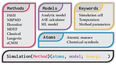
The Simulation holds the static parameters of the system such as the atom types, temperature and simulation cell. Further, its type parameter (Method in Fig. 1) acts as a label that determines the dynamics method. These Methods are regular Julia structsjul a and can be defined to contain any extra parameters. In this way, the Simulation type has a basic structure for shared functionality between dynamics methods, but allows for arbitrary extension through the Method parameter. By defining a new Method, multiple dispatch can be used to modify and implement functions to perform new dynamics methods.
Another goal of the package is to facilitate easier comparison with existing methods. Currently, this is challenging as implementations for many prototype dynamics methods are not publicly available and can be difficult to obtain. We provide implementations of many methods, along with detailed descriptions of the implementation specifics. In this way, the package can be used as a resource for obtaining benchmark data and as an educational resource that provides extra computational details, so that those details do not have to be covered in the supporting information of publications.
Finally, the prototype implementations must be easily transferable for both model Hamiltonians and realistic atomistic systems. Generally, there is a disconnect between research codes and large production applications that can lead to a duplication of effort when the developer must re-implement functionality in a more efficient or scalable format. The key difference between simple models and atomistic problems lies in the evaluation of the electronic Hamiltonian. The underlying dynamics to propagate the motion of atoms is identical. We can take advantage of this similarity by abstracting the dynamics from the electronic problem, exposing a simple interface for defining the Hamiltonian. This interface is packaged separately as NQCModels.jl and included as a dependency. By separating the interface, the models can be accessed individually and integrated into other codes.
NQCD simulations involve the calculation of observables over many trajectories. The initial coordinates for each trajectory are sampled from an appropriate distribution, before propagating the coordinates and momenta in time. During the propagation, at each timestep, the electronic Hamiltonian is evaluated as a function of the nuclear coordinates. The following sections discuss how each of these aspects is handled by NQCDynamics.jl by following the simulation workflow presented in Fig. 2.

III.1 Preparing initial conditions
Before performing dynamics simulations, it is important to ensure the initial nuclear and electronic distributions are sampled correctly, otherwise the trajectories become meaningless. Within NQCDynamics.jl, the submodule InitialConditions provides the functionality to generate these initial distributions. For simulations where the initial nuclear distribution is at thermal equilibrium we provide Monte Carlo sampling and dynamics using a Langevin thermostat.Tuckerman 2010 Both of these methods have also been implemented in the path-integral form, which exploits the ring polymer normal mode representation to more efficiently sample the ring polymer phase space. Ceriotti et al. 2010; Tuckerman 2010; Korol, Bou-Rabee, and Miller 2019; Korol et al. 2020 For non-equilibrium nuclear distributions, we have implemented Einstein-Brillouin-Keller (EBK) quantisation for diatomic molecules,Larkoski, Ellis, and Curtis 2006 which generates semiclassical distributions with given vibrational and rotational quantum numbers and provides initial conditions for diatomic gas-surface scattering dynamics. In addition to these methods, we provide simple analytic distributions built on top of Distributions.jl.Besançon et al. 2021 These include the Boltzmann velocity distribution, Wigner distributions for the quantum harmonic oscillator, and a ring polymer in a harmonic potential. The above methods are used to sample the nuclear degrees of freedom separately from the electronic variables. For all methods, the electronic variables are sampled analytically or set to represent a specific initial state. Currently, we provide only for initial conditions where the nuclear and electronic distributions are separable, allowing for individual sampling of each subsystem. In summary, the currently available sampling methods to create initial conditions include:
- •
Einstein-Brillouin-Keller quantisationLarkoski, Ellis, and Curtis 2006
- •
Langevin molecular dynamics (BAOAB algorithm)Tuckerman 2010; Leimkuhler and Matthews 2013a; Leimkuhler and Matthews 2013b
- •
Path integral Langevin dynamics (BCOCB algorithm)Korol, Bou-Rabee, and Miller 2019; Korol et al. 2020
- •
Metropolis-Hastings Monte CarloTuckerman 2010
- •
Path integral Monte CarloTuckerman 2010
III.2 Performing dynamics
Each of the trajectory-based dynamics methods can be formulated as a set of coupled differential equations. Given the variety of differential equations that we must solve, it is easiest to use an established library for solving them, rather than implementing new algorithms and integrators for every dynamics method. This becomes especially relevant when developing new methods where, initially, the specific properties of the integration algorithm are not yet a priority. In Julia, the DifferentialEquations.jl packageRackauckas and Nie 2017 provides a variety of algorithms for the numerical integration of differential equations. We have hence chosen to use DifferentialEquations.jl as the main driver for our dynamics simulations. With this choice, we need only define a function that evaluates the time-derivative of each of the dynamical variables that we can pass to any of the available solvers (defined in DynamicsMethods, Fig 2). Listing 3 shows the implementation of this function for the eCMM method (Sec. IV.1.5).
In some cases, such as when using ring polymer methods, there are specialised algorithms available that allow for larger timesteps and improved performance.Korol, Bou-Rabee, and Miller 2019; Korol et al. 2020 Although not immediately available from DifferentialEquations.jl, the implementation of additional integration algorithms is well documented in the online manual and, once implemented, they can be directly compared to the library of existing algorithms. We have taken this approach to implement versions of the MIntChurch et al. 2017 and BCOCBKorol, Bou-Rabee, and Miller 2019; Korol et al. 2020 algorithms within DifferentialEquations.jl to efficiently integrate mapping variable and ring polymer dynamics, respectively.
As shown in Fig. 2, two functions are used to launch dynamics simulations: run_trajectory and run_ensemble. The former is used to perform a single trajectory at a time, whereas the latter can be used to perform multiple trajectories in parallel. The choice between the two ties directly into the output quantities from the dynamics (Fig. 2). In the single trajectory case, quantities of interest (positions, momenta, etc.) can be output at specified intervals. This functionality is also available from the ensemble interface, but there is the further option to request more complex observables, such as scattering probabilities or time-correlation functions. In doing so, it is possible to reduce the output as the trajectories finish, saving memory and reducing the burden of handling large amounts of data.
The parallelism available in the ensemble mode is provided by DifferentialEquations.jl and allows trajectories to be performed simultaneously using both shared memory and distributed memory parallelism. For large scale simulations on high performance computing facilities, the distributed form allows the user to leverage multi-node clusters to perform a large number of trajectories. To demonstrate the effectiveness of the parallelism we have included a scaling study (Fig. 4) carried out on a system equipped with Dell PowerEdge C6420 compute nodes with 48 cores each. These results were obtained by measuring the time taken to perform trajectories using compute cores. The simulations were carried out as described in Sec. IV to obtain the eCMM result for model B. When using the simulation time span in Sec. IV, , the efficiency begins to deteriorate when using more than 48 cores (1 node). However, when increasing the simulation time span to , we see that the efficiency remains high across multiple nodes. This suggests that we are capable of achieving almost perfect scaling up to 768 cores (16 nodes), assuming that the time taken to simulate each trajectory is long enough to render the parallel overhead negligible.

Inside the DynamicsMethods submodule, the following dynamics methods are currently implemented:
- •
Classical molecular dynamicsTuckerman 2010
- •
Molecular dynamics with electronic friction (MDEF)Head-Gordon and Tully 1995; Maurer et al. 2016a
- •
Ehrenfest molecular dynamics McLachlan 1964; Subotnik 2010; Choi and Vaníček 2021
- •
Fewest-switches surface hoppingTully 1990a
- •
Ring polymer molecular dynamics (RPMD)Craig and Manolopoulos 2004; Habershon et al. 2013
- •
Nonadiabatic RPMD (NRPMD) Richardson and Thoss 2013; Richardson et al. 2017; Chowdhury and Huo 2019; Chowdhury and Huo 2021
- •
Centroid ring polymer surface hopping (RPSH) Shushkov, Li, and Tully 2012; Shakib and Huo 2017
- •
Centroid ring polymer Ehrenfest dynamics Yoshikawa and Takayanagi 2013
- •
Extended classical mapping model (eCMM) He and Liu 2019; He et al. 2021a
- •
Generalized spin mapping approach Runeson and Richardson 2019; Runeson and Richardson 2020
III.3 Defining the Hamiltonian with NQCModels.jl
The final part of Fig. 2 that has not yet been described is the NQCModels.jl package. This package is responsible for providing the dynamics code with the potential energy surfaces that define the system interactions. In the case of analytic diabatic models, among others, these include Tully’s two-state scattering models,Tully 1990a Coronado and Miller’s three-state Morse potentials,Coronado, Xing, and Miller 2001 and the spin-boson model.Nitzan 2006 However, the package can also define or interface with high-dimensional atomistic models and ab initio Hamiltonians. We accomplish this by exposing a minimal set of functions that are required to take the nuclear positions and return the electronic quantities. The developer is free to wrap any code within these functions to perform the necessary computations. The flexible interface provided by NQCModels.jl is largely responsible for the system-size agnostic structure of the dynamics code.
The modular design that Julia affords means that these models can be used separately from the dynamics code if desired, e.g. to compute energy values or to be incorporated into other codes. Fig. 5 shows the layout of the NQCModels.jl package. The top row shows the basic models and interfaces included in the package itself. The bottom row shows some of the child packages that implement the interface to provide add-on models. These extra models are tailored for specific applications and are packaged separately. For example, NNInterfaces.jl provides the on Ag(111) neural network model used in Sec. V. The advantage of this format is that NQCModels.jl can remain lightweight, with minimal dependencies, and add-on packages have more freedom as they operate separately from the main package.

One of the included interfaces is to the Atomic Simulation Environment (ASE)Hjorth Larsen et al. 2017 written in Python that provides a library of calculators that give energies and forces using a variety of electronic structure programs. Using PyCall.jl we are able to directly access Python from within Julia. With this, we have implemented a simple wrapper for ASE calculators that allows us to access the values provided by ASE with minimal overhead. In principle, this interface can be used with any ASE calculator as easily as in native Python.Hjorth Larsen et al. 2017 This provides capabilities to perform on-the-fly dynamics with a vast array of electronic structure and quantum chemistry codes that have existing calculator instances within ASE. It also provides access to atomistic machine learning (ML) packages via ASE, such as QUIP/GAPCsányi et al. 2007; Bartók et al. 2010 and SchNetPackSchütt et al. 2018; Schütt et al. 2019. Both packages provide an ASE calculator instance that can be exposed to NQCDynamics.jl via our interface.
For atomistic molecular dynamics simulations, ML has become a key tool to facilitate dynamics of large systems or dynamics over long time-scales.Deringer et al. 2021; Li et al. 2021 More recently, ML models of excited-state properties and whole Hamiltonians have become available Westermayr et al. 2019; Schütt et al. 2019; Zhang et al. 2022 There has been substantial recent progress in machine learning with JuliaInnes 2018; Blaom et al. 2020; Gao et al. 2020b. For example the ACE.jl packageDrautz 2019; Dusson et al. 2021 provides for the parametrization of interatomic potentials based on the Atomic Cluster Expansion. Nevertheless, most existing atomistic ML models are developed and trained using other languages. Through Julia’s language interoperability features,Bezanson et al. 2017 we connect to these models with minimal difficulty. The H2 on Ag(111) model in NNInterfaces.jl (Sec. V) relies upon a Fortran libraryJiang and Guo 2014a. By directly calling the functions compiled into this library using ccall,jul c we are able to access the potential, forces, and electronic friction tensor from the same interface as the analytic models.
III.4 Example script
Now that we have introduced the fundamentals of the package, we can introduce a basic script that shows how each of the components work together. The example script (Listing 6) performs a single trajectory with classical molecular dynamics in a 1D harmonic potential. The structure of this script is typical for all dynamics simulations using NQCDynamics.jl.
In Listing 6, line 1 imports the package. using NQCDynamics brings both the module name and all exported symbols into the global namespace.jul d Line 3 creates the atoms which tells the simulation which particles are in the system. Line 4 creates the model. In this example, Harmonic is a 1D harmonic potential, but can be replaced by any type that implements the NQCModels.jl interface. Line 7 shows the creation of the simulation, which is the central parameter type for all simulations (Fig. 1). This contains all of the static parameters of the system, which in this case, are the atoms and the model that defines their interactions. The Method type parameter, here Classical, is how the user chooses the dynamics method they will use, this can be any of the implemented dynamics methods. After creating the simulation, the dynamical variables are created. For classical dynamics, these are the positions and momenta but will contain electronic variables when performing nonadiabatic dynamics. The velocities and positions are provided as matrices with the number of degrees of freedom per atom along the first dimension and the number of atoms along the second dimension. The simulation time span is defined on line 17 to be . By default, all quantities are assumed to be in atomic units, however, Unitful.jlUni can be used to attach alternative units which are converted internally. Finally, the simulation is performed using run_trajectory. After execution, the output trajectory is a table containing the values for the positions and velocities at each timestep. The interface described here is similar for all dynamics methods, making it easy to switch between and compare different methods. Interfacing with the package via a Julia script means that the user has the ability to use any Julia functionality to manipulate inputs and outputs. This affords great flexibility when considering future developments.
In the preceding sections, we have provided motivation for using NQCDynamics.jl and described its functionality. NQCDynamics.jl is open-source and freely available on GitHub.NQC a The package documentation and tutorials are hosted online with GitHub pages and are updated with each release.NQC b The documentation provides a comprehensive introduction for new users along with implementation details and code specifications useful for developers. For each of the implemented methods, the theoretical background is introduced alongside walkthrough examples that aim to reproduce published results. In the following sections, we will present two example use cases for NQCDynamics.jl.
IV Example I: Non-equilibrium population dynamics of the spin-boson model
In this example we will use NQCDynamics.jl to evaluate quantum time-correlation functions Berne and Harp 1970; Nitzan 2006; Hele 2017; Bonella, Montemayor, and Coker 2005 of the form
| (1) |
where is the trace over both the nuclear and electronic subsystems and and are arbitrary quantum operators. is the Hamiltonian operator of the full system. Depending on the identity of the operators and , these correlation functions can be used to calculate reaction rates, spectra, and various transport coefficients.Berne and Harp 1970; Hele 2017 Correlation functions of this form are typically challenging to evaluate using a quantum mechanically exact formalism but it is possible to approximate the quantum dynamics by using mixed quantum-classical and semiclassical dynamics.
In the following, the theory will be presented for a general Hamiltonian with electronic states in the diabatic representation:
| (2) |
Here, and are vectors of position and momentum operators and is the diagonal mass matrix. Throughout we will be using bold notation for vectors and matrices. are the diabatic potential energy surfaces and is the coupling between the two states . In this section, we explore the case where and such that the correlation function can be viewed as the time-dependent population of state starting from a given initial density . This initial density is separable into the nuclear and electronic parts, where is the thermal equilibrium nuclear distribution of the ground state, and the electronic population starts in state .
| (3) |
In the next section we will briefly introduce a set of dynamics methods that are implemented in the package that can be used to approximate the population time-correlation function (Eq. 3). Each of these methods takes a trajectory based approach, where initial conditions are sampled from a distribution and propagated using the appropriate algorithm to evaluate the population at later time.
IV.1 Methods
IV.1.1 Fewest switches surface hopping (FSSH)
Tully’s fewest-switches surface hopping (FSSH) method Tully 1990b; Tully 1991; C. Tully 1998 is one of the most frequently used methods, implemented in many programs, for simulating coupled electron-nuclear dynamics in molecular systems. Barbatti et al. 2014; Barbatti et al. 2018; Mai, Marquetand, and González 2018; Mai et al. 2018 In recent years, there have been several investigations focused on testing its efficacy in the condensed phase Chen and Reichman 2016a and for modelling molecules on surfaces. Dou and Subotnik 2020; Shenvi, Roy, and Tully 2009; Jin and Subotnik 2021 Here we will shortly summarize how it can be used to approximate time-correlation functions of the form introduced above.
In FSSH, the nuclei are described by the classical time-dependent Hamiltonian:
| (4) |
Note that the symbols have no hats as they represent classical variables, not quantum operators. is the energy of the -th adiabatic state obtained by diagonalising the electronic Hamiltonian. The time-dependent quantity is the discrete state variable that takes on the integer value of the currently occupied adiabatic state. To obtain the value of , the time-dependent Schrödinger equation is propagated alongside the classical equations of motion for the nuclei. In the adiabatic basis, this equation can be cast in terms of the wavefuction expansion coefficients as
| (5) |
where is the nonadiabatic coupling vector between states and . The basic assumption made in FSSH is that the nuclei move on one adiabatic potential energy surface at a time, as illustrated by the Kronecker delta in equation 4. After every time step, the probability to make a transition to another state is evaluated. Such a transition is called a hop and its success is determined by comparing the hopping probability to a uniform random number. If the computed hopping probability is larger than the random number, a hop takes place and the value of changes. Typically, the hopping probability is evaluated based on nonadiabatic couplings Tully 1991; Mai et al. 2018, but other approximate schemes have also been proposed.Zener 1932; Zhu, Kamisaka, and Nakamura 2002 We have implemented the hopping probability according to Subotnik et al. 2016 which is based on the original notion of nonadiabatic couplings between adiabatic potential energy surfaces. NQCDynamics.jl implements the hopping procedure using callback functions from DifferentialEquations.jl.Rackauckas and Nie 2017 Listing 7 shows the implementation of a general surface hopping procedure in our package. The HoppingCallback is given to the solver, which after every timestep performs the surface hopping. This callback approach decouples the discontinuous hopping events from the continuous dynamics and allows users to investigate alternative hopping schemes by re-implementing individual functions that appear in Listing 7. For example, different velocity rescaling procedures can be implemented by modifying the rescale_velocity! function.
Since FSSH is a mixed quantum-classical method, the most appropriate approximation to Eq. 3 is the partially Wigner transformed expression:Sergi and Kapral 2004; Hsieh and Kapral 2013
| (6) |
is the number of nuclear degrees of freedom, is the Wigner transformed nuclear density, and are the populations of state obtained from surface hopping trajectories at time . Recall that we are interested in the populations of the diabatic states, though we perform FSSH in the adiabatic representation. We calculate the diabatic populations using the mixed quantum classical density approach.Landry, Falk, and Subotnik 2013; Chen and Reichman 2016b Numerical evaluation of Eq. 6 involves performing FSSH trajectories sampled from and averaging the population over all trajectories.
IV.1.2 Ring polymer surface hopping (RPSH)
For FSSH, we are using the Wigner distribution to initialise the nuclear configurations. However, the Wigner distribution is difficult to sample for realistic systems, Liu and Miller 2009; Vázquez, Talapatra, and Geva 2011 and the classical propagation does not conserve the initial distribution, leading to zero point energy leakage. Habershon and Manolopoulos 2009 A possible solution to these problems is to use ring polymer surface hopping (RPSH).Shushkov, Li, and Tully 2012; Shakib and Huo 2017 Ring polymer molecular dynamics (RPMD) uses the imaginary-time path integral formalism to map the quantum distribution of the nuclei onto the extended phase space of a classical ring polymer to approximate the simulation of real-time correlation functions.Craig and Manolopoulos 2004; Habershon et al. 2013 The ring polymer is comprised of multiple replicas of the nuclei, each joined by harmonic springs with stiffness depending on the temperature and mass of the particle. At low temperatures and light particle masses, the springs become softer, leading to a swelling of the ring polymer and a particle that incorporates quantum effects such as zero point energy and, to a more limited extent, tunneling. At high temperatures, the stiff springs cause the polymer beads to coalesce, becoming equivalent to a classical particle. The key advantage of ring polymer dynamics is that the quantum Boltzmann distribution is conserved.
RPSH is an ad hoc combination of trajectory surface hopping and RPMD. The algorithm follows FSSH, except the classical nuclear dynamics are replaced by the ring polymer dynamics. However, the additional complexity of the ring polymer leads to some ambiguity in the implementation of the propagation of the electronic quantities and the rescaling of the momenta. Two options for treating this ambiguity exist: the bead and centroid approximations.Shushkov, Li, and Tully 2012 The bead approximation involves evaluating the electronic quantities for every bead and using each contribution to propagate the electronic quantities. The centroid approximation simply replaces the classical particle in the FSSH algorithm with the ring polymer centroid. When rescaling the momenta, the bead approximation conserves energy for the entire ring polymer, whereas the centroid approximation conserves energy only for the centroid. The method we use here is the centroid approximation since it is more convenient and previous results have shown little difference in results between both approaches.Shakib and Huo 2017
As with FSSH, the nuclear dynamics follow a classical Hamiltonian:
| (7) |
This Hamiltonian matches equation 4, with the addition of replicas, where each replica is joined to the adjacent with a harmonic spring. Since this is a ring polymer, the indices are cyclic and the final replica is connected to the first. The spring frequency is directly proportional to the temperature as where . Other than the nuclear dynamics, RPSH proceeds exactly as FSSH in the approximation of equation 3, with the exception that the initial distribution is taken as the thermal ring polymer distribution .
| (8) |
As with all of the methods, this integral is evaluated by simulating an ensemble of trajectories and averaging the populations. The populations are obtained as for FSSH, except that the ring polymer centroids replace the classical nuclei.
IV.1.3 Ehrenfest molecular dynamics
As an alternative to surface hopping dynamics, a mean-field approach can be taken such that the force is averaged over all states, weighted by the electronic populations. McLachlan 1964; Subotnik 2010; Choi and Vaníček 2021 The Ehrenfest Hamiltonian can be written as
| (9) |
Note that here, in contrast to FSSH and RPSH, the time-dependence of the classical Hamiltonian comes directly from the electronic coefficients , rather than from an auxiliary state variable. As with the surface hopping methods however, the electronic Schrödinger equation must be integrated alongside the Hamiltonian dynamics with Eq. 5. Since Ehrenfest is another mixed quantum-classical method, it approximates Eq. 3 exactly as FSSH and we can use Eq. 6. The evaluation of the populations is simplified here and comes directly from the electronic coefficients after conversion to the diabatic representation.
IV.1.4 Ehrenfest ring polymer molecular dynamics
As with FSSH, the same discussion surrounding the choice of initial nuclear distribution applies and the drawbacks of the Wigner distribution are still present. Similarly, we can introduce an ad hoc ring polymer formalism here to tackle the same problem. Yoshikawa and Takayanagi 2013 We can directly follow the RPSH treatment for the electronic degrees of freedom (propagating the electronic equation of motion for the centroid), but obtain the nuclear forces from the Ehrenfest approach as described by the Hamiltonian:
| (10) |
The dynamics of this Hamiltonian can be seen as a straightforward replacement of the classical nuclei of Ehrenfest dynamics with the classical ring polymer.
IV.1.5 Extended classical mapping model (eCMM)
The classical mapping methods introduced in the following sections take a different approach to the mixed quantum-classical methods discussed previously. These methods seek to treat the nuclear and electronic degrees of freedom on equal footing by mapping the discrete electronic states onto continuous degrees of freedom, then taking the semiclassical limit. Many of the existing approaches are based upon the work of Meyer and MillerMeyer and Miller 1979 and later Stock and ThossStock and Thoss 1997 where the electronic degrees of freedom become the Meyer-Miller-Stock-Thoss mapping variables. More recently, a unified framework has been introducedLiu 2016 from which many existing mapping methods can be derived, including the Meyer-Miller Hamiltonian.
From the unified framework, the extended classical mapping model He and Liu 2019; He et al. 2021a; He et al. 2021b uses the Meyer-Miller Hamiltonian:
| (11) |
Here, and are the electronic mapping variables for state and is a parameter that can take any value greater than .
The eCMM population correlation function is
| (12) |
where denotes integration over the constraint space
| (13) |
To evaluate this integral, the nuclear degrees of freedom are sampled from the Wigner distribution and the electronic degrees of freedom are sampled such that the constraint in Eq. 13 is satisfied. This is equivalent to sampling on the surface of a dimensional hypersphere with radius . Trajectories are then obtained using Eq. 11 to calculate the correlation at time . Although not presented in this article, the similar spin mapping methods introduced by Runeson and Richardson 2019; Runeson and Richardson 2020 have been compared to the eCMM methodHe et al. 2021b and are equivalent for certain choices of .
IV.1.6 Nonadiabatic ring polymer molecular dynamics (NRPMD)
As with FSSH, an RPMD extension to classical mapping dynamics has been proposed, referred to as nonadiabatic ring polymer molecular dynamics (NRPMD). Richardson and Thoss 2013; Richardson et al. 2017; Chowdhury and Huo 2019 NRPMD uses the Meyer-Miller representation for the electronic degrees of freedom and the ring polymer path-integral discretisation for the nuclear degrees of freedom. However, unlike the surface hopping alternative, NRPMD has rigorous mathematical justification through its links to the recently derived nonadiabatic Matsubara dynamics.Chowdhury and Huo 2021 This formal theoretical footing helps to justify its implementation and removes some of the ambiguities encountered in methods such as RPSH.
The NRPMD Hamiltonian is given by
| (14) |
which bears much resemblance to the classical Meyer-Miller Hamiltonian in Equation 11. Usually this Hamiltonian is presented such that , though it has been provided here in a more general form to emphasise the similarity to the Meyer-Miller Hamiltonian.
The NRPMD population time-correlation function is
| (15) |
with the population estimator
| (16) |
As with the other ring polymer methods, the initial nuclear configuration is sampled from the thermal ring polymer distribution . The electronic variables are sampled according to the procedure detailed in ref. 37, which differs from the approach used above for eCMM. This methodology for sampling the electronic variables and evaluating the population follows the work of Chowdhury and HuoChowdhury and Huo 2019, though more recently an alternative form has been presentedChowdhury and Huo 2021 that more closely matches previous work with Meyer-Miller mapping dynamics. Gao et al. 2020a; Saller, Kelly, and Geva 2021 When using only a single bead for NRPMD, the method becomes equivalent to the LSCI of Gao et al. 2020a with focused initial conditions.Runeson and Richardson 2019
IV.1.7 Ring polymer extended classical mapping model
Before we apply all of these methods to a model system in the coming sections, it is interesting to consider how one might replace the nuclear dynamics of eCMM with ring polymer dynamics. Although not rigorously justified, the flexible structure of NQCDynamics.jl allows us to explore heuristic methods such as this and evaluate their effectiveness via numerical tests.
If we assume the system is described by the NRPMD Hamiltonian in Eq. 14, then we must adapt Eqs. 12 and 13 in line with the extended ring polymer phase space. Since we have copies of each mapping variable, we can simply include the extra variables in the constraint summation such that the total population remains conserved.
| (17) |
Then, in the spirit of the NRPMD population estimator (Eq. 16), we can rewrite the correlation function with populations accumulated over all the beads.
| (18) |
IV.2 Spin-boson model
To compare each of the methods introduced in the previous section, we will use the spin-boson model. This model is comprised of a two-state system coupled to a bath of harmonic oscillators where the couplings and bath frequencies are characterised by a given spectral density . The model describes a dissipative quantum system and has been widely used as a benchmark for approximate nonadiabatic methods due to the feasibility of computing numerically exact quantum results. Thoss, Wang, and Miller 2001; Wang, Thoss, and Miller 2001; Berkelbach, Reichman, and Markland 2012; Rekik et al. 2013; Habershon 2013; He and Liu 2019; Gao et al. 2020a; Sindhu and Jain 2021 The spin-boson Hamiltonian can be written in the form of Eq. 2 by setting
| (19) |
and taking the mass matrix to be the identity matrix. In the potential operator , is the energy bias between the two states and is the coupling between them. The couplings to the position operators and the diagonal matrix of oscillator frequencies are obtained by discretisation of the spectral density.
In this work, we employ the Ohmic spectral density:
| (20) |
which can be discretised to giveHe and Liu 2019
| (21) | ||||
| (22) |
with . For all simulations we set .
Different regimes of the model can be explored by modifying the relationship between the parameters. The model is symmetric when and asymmetric otherwise. The system-bath coupling strength is determined by the reorganisation energy . The temperature regime is characterised by the relationship between and : the high temperature regime is encountered when and the low temperature regime when . The balance between the adiabatic and nonadiabatic regimes is determined by and . In the case of the model represents the adiabatic regime, for it represents the nonadiabatic regime. Throughout, and the parameters and alone will determine the regime of the model. When both and are large, this is the regime where both nuclear quantum effects and nonadiabatic effects become significant.
For this model, the initial nuclear density is given by the bath at thermal equilibrium:
| (23) |
with the bath Hamiltonian
| (24) |
It is possible to sample the corresponding Wigner and ring polymer distributions analytically. The Wigner distribution is a normal distribution of the form:
| (25) |
with .Runeson and Richardson 2019 The ring polymer distribution can be sampled in the ring polymer normal mode coordinates with the expression
| (26) |
where and is the frequency of the -th normal mode. This can be converted back to the primitive coordinates using the standard ring polymer normal mode matrix.Ceriotti et al. 2010
IV.3 Simulation details
The results in the next section were obtained by performing trajectories for each of the methods, sufficient for numerical convergence for all methods to the relevant accuracy. For NRPMD, the parameter was set equal to as is consistent with previous work Richardson and Thoss 2013; Chowdhury and Huo 2019 and for eCMM it is set to as done previously.He and Liu 2019 A recent investigation into the value of suggests the effect is minimal for reasonable values.He et al. 2021a For the ring polymer simulations, 50 beads were used to obtain converged results. However, for the ring polymer Ehrenfest and RPSH, using only a single bead was capable of reproducing the same population dynamics. We believe that this behaviour is specific to the fact that we are using centroid approximations and that the nuclear degrees of freedom are harmonic. The Wigner methods were integrated using the Vern7 solver,Verner 2010; Rackauckas and Nie 2017 whilst the ring polymer methods used variants of MIntChurch et al. 2017 and Tsit5Tsitouras 2011 coupled with normal mode propagation for the ring polymer. Ceriotti et al. 2010; Korol, Bou-Rabee, and Miller 2019; Korol et al. 2020 The fixed timestep methods used a timestep of whereas the adaptive Vern7 used relative and absolute tolerances of .
IV.4 Results and discussion
We have applied the methods described above to the five spin boson models A, B, C, D and E with parameters in Table 1.Gao et al. 2020a The first four models (A-D) have been previously investigated in the benchmark study of Gao et al. Gao et al. 2020a and the final model (E) with elevated system-bath coupling appears in the work of Wang et al. Wang, Thoss, and Miller 2001
For each method, we present two variants characterised by the representation used to model the nuclear degrees of freedom, either the Wigner or ring polymer representation. We evaluate which is the time dependent population difference between the two spin states. The numerically exact results for models A-D were calculated using the dissipation equation of motion method and are taken from the benchmark study of Gao et al.Gao et al. 2020a Similarly, the exact result for model E is taken from Ref. 125 and was calculated using the multiconfiguration time-dependent Hartree approach.
| Model | Description | ||||
|---|---|---|---|---|---|
| A | Symmetric, high temperature | 0 | 0.09 | 2.5 | 0.10 |
| B | Symmetric, low temperature | 0 | 0.09 | 2.5 | 5.00 |
| C | Asymmetric, high temperature | 1 | 0.10 | 1.0 | 0.25 |
| D | Asymmetric, low temperature | 1 | 0.10 | 2.0 | 5.00 |
| E | Symmetric, high temperature | 0 | 0.50 | 10.0 | 0.25 |
For the symmetric, high temperature model A (Fig. 8, left column), all methods are capable of reproducing the exact population dynamics. In fact, due to the high temperature nature of the model, the ring polymer dynamics requires only a single bead to reach convergence for all methods. Since the Wigner distribution converges to the classical Boltzmann distribution at high temperature, it is expected that the results be identical to the ring polymer dynamics.
For the asymmetric, high temperature model C (Fig. 8, second column), only eCMM is capable of capturing the exact result, with both FSSH and RPSH coming close. Both Ehrenfest variants perform worse, failing to capture the long time population. For this model, NRPMD returns the same result as (RP)Ehrenfest. Its single bead Wigner counterpart, LSCI, slightly overestimates the long-time population difference. For RPSH and ring polymer Ehrenfest, a single bead was sufficient to converge the dynamics, as expected for a high temperature model, where the methods become equivalent to their classical counterparts. However, the two ring polymer mapping methods (NRPMD, RPeCMM) differ significantly from their classical variants, this is likely due to the addition of extra electronic variables. The additional electronic variables mean that even when the ring polymer shrinks to a classical particle, the method is not equivalent to the single bead version.

With the low temperature models (Fig. 9), the difference between the ring polymer and Wigner methods is more pronounced than in the high temperature case (Fig. 8). Using the symmetric model B (Fig. 9, first column), RPSH and ring polymer Ehrenfest perform worse than their Wigner counterparts which are able to reproduce the exact dynamics. The RP variants exhibit dynamics with slower decoherence time. Similarly, eCMM also reproduces the exact dynamics, but its ring polymer version overestimates the amplitude of the Rabi oscillations. However, the decoherence time appears faster than in RPSH comparable to RPEhrenfest. In contrast, LSCI underestimates the amplitude while its ring polymer extension NRPMD matches the exact result. Across all methods, the oscillation amplitude is greater for the ring polymer variants.
Model D (Fig. 9, second column), the low temperature asymmetric model, is the most challenging for our approximate methods. As seen across all models, the exact dynamics is captured comfortably at short times, but here, the long-time limit is out of reach for all methods except eCMM, which captures close to exact dynamics across all times. For the two low temperature models, all ring polymer method variants overestimate coherence during the dynamics.

The first four models have relatively weak system-bath coupling (), whereas model E (Fig. 10) has a larger value of . For this model, we see that none of the methods are capable of recovering the exact dynamics, although eCMM is the closest. Compared to the ring polymer methods, the short-time dynamics of the Wigner methods is more accurate, though a similar level of accuracy is observed at later time. The Wigner methods all underestimate the rate of population transfer, but the ring polymer methods (except for NRPMD) instead overestimate the decay.

Considering that the ring polymer modifications necessarily increase the computational expense of each method, significant improvements in the dynamics are required to justify their use. However, reviewing the results for all of the models suggests that the ring polymer dynamics cannot be reliably expected to immediately improve the population dynamics. For the low temperature models, improvement is seen only for NRPMD in model B. In all other cases, the ring polymer modification has no effect, or leads to small changes that do not directly improve the result.
Using the Wigner distribution reliably gives strong results across all five models, especially in the case of eCMM. Unfortunately, sampling the Wigner distribution for realistic atomistic systems is more challenging than the corresponding ring polymer distribution. Liu and Miller 2009; Vázquez, Talapatra, and Geva 2011 The high temperature results here (Fig. 8) suggest that the ring polymer methods are adequate substitutes in this regime, often requiring very few beads to obtain similar results. However, at low temperature, the ring polymer methods appear less capable of achieving the accuracy afforded by the Wigner methods.
In the benchmark study of Gao et al.Gao et al. 2020a these models (A-D) were investigated using a collection of classical mapping methods using the Wigner distribution. The only methods we have used that also appear in their work are Ehrenfest and LSCI, where the results are identical. The most effective methods in their study are the LSC methods with modified population estimators that align very closely with the eCMM results presented here.
The NQCDynamics.jl code allows us to study all these method variants on equal footing and to systematically analyse the impact of different approximations and parameter choices. This will facilitate future method improvements to achieve accurate long-term dynamics in realistic atomistic systems.
V Example II: Reactive Scattering of H2 on Ag(111)
In addition to the model Hamiltonian quantum dynamics of the first example, NQCDynamics.jl also allows us to investigate full dimensional atomistic systems. This example focuses on reproducing and augmenting the work of Zhang et al. 2019 where they investigated the effect of hot-electrons during the reactive scattering of on a Ag(111) surface. In this system, nonadiabatic effects arise from the interaction of the molecular motion with the electronic bath of the metal substrate. Traditional adiabatic molecular dynamics evolving on a single potential energy surface ignores these effects, however, molecular dynamics with electronic friction (MDEF)Head-Gordon and Tully 1995 has been proposed as an alternative that attempts to approximately include these effects by introducing additional frictional forces due to the nonadiabatic interactions between adsorbate atoms and metal electrons. In the previous study,Zhang et al. 2019 the reactive scattering was investigated using machine learning to describe both the potential energy surface and the electronic friction.Zhang et al. 2019; Jiang and Guo 2014b; Maurer et al. 2017; Maurer et al. 2019 After a brief overview of the different flavours of MDEF, using these same machine learning modelsZhang et al. 2019; Jiang and Guo 2014b we investigate the dissociative chemisorption and state-to-state scattering of on Ag(111).
V.1 Molecular Dynamics with Electronic Friction
Molecular dynamics with electronic friction (MDEF) is a quasi-classical method that uses a Langevin equation to approximate weak nonadiabatic effects encountered at metal surfaces.Alducin, Díez Muiño, and Juaristi 2017; Head-Gordon and Tully 1995 Within this theoretical framework, the coupling between the molecular degrees of freedom and the electron-hole pair excitations within the metal substrate is described by means of frictional and stochastic forces.Head-Gordon and Tully 1995; Maurer et al. 2016b In doing so, the dynamical effects that arise due to the complex electronic structure of the metal are condensed into a single electronic friction coefficient or friction tensor in the case of multidimensional dynamics.Head-Gordon and Tully 1995; Alducin, Díez Muiño, and Juaristi 2017; Maurer et al. 2016b
During MDEF, the total nuclear force is given by:
| (27) |
The first term on the right hand side of Eq. 27 corresponds to the conservative force associated with the adiabatic potential energy surface. Adiabatic molecular dynamics simulations are governed solely by this unique ground-state force. The second term describes the energy losses produced by adsorbate-substrate interaction, with magnitude proportional to the friction tensor and the particle velocity . The final term is a temperature and friction-dependent stochastic random force that satisfies the fluctuation-dissipation relation.
Light-driven molecular dynamics processes can also be simulated using MDEF.Scholz et al. 2019; Alducin et al. 2019; Serrano Jiménez et al. 2021 In this context, an external laser source is incorporated within the nuclear dynamics by modifying the temperature in the random force term as a function of time.Scholz et al. 2019; Serrano Jiménez et al. 2021 The temperature is chosen to model the electronic temperature which is often described by a simple 1D two-temperature model.Anisimov, Kapeliovich, and Perel’Man 1974 Further improvements of the dynamics can be also found by including the coupling with bulk phonons through a generalised Langevin oscillator model, but the relevance of the phonon dissipation effects on the final nuclear dynamics depends on the studied system.Scholz et al. 2019; Serrano Jiménez et al. 2021; Zhu et al. 2020 In the example case of H2 scattering dynamics on a Ag(111) surface, we will explicitly ignore phonon dissipation effects.
MDEF simulations are usually performed using one of two methods for calculating the electronic friction tensor. The following sections describe the two choices and discuss the details of their implementation.
V.1.1 Local density friction approximation (LDFA)
The simplest version of MDEF uses a local density friction approximation (LDFA) where a single friction coefficient is associated with each adsorbate atom based on the local electron density of the bare metal substrate.Alducin, Díez Muiño, and Juaristi 2017; Scholz et al. 2019 During the dynamics, the local density is computed as a function of each adsorbate coordinate , which is then converted to a friction coefficient via a fitting of pre-computed values. Analytic expressions are commonly used to fit the pre-computed valuesScholz et al. 2019; Scholz et al. 2016 but our implementation uses a cubic spline to fit the LDFA values reported by Gerrits and Meyer.Gerrits, Juaristi, and Meyer 2020
With this, the friction tensor becomes diagonal:
| (28) |
In this way, the fitting function allows us to connect any point visited by the adsorbate atoms with a single electronic friction coefficient used to drive the nuclear dynamics. LDFA friction coefficients have previously been widely used to describe surface processes such as atomic and molecular diffusion and laser-driven dynamics.Juaristi, Alducin, and Saalfrank 2017; Scholz et al. 2019; Alducin, Díez Muiño, and Juaristi 2017
V.1.2 Orbital-dependent electronic friction (ODF)
A more general formulation of the electronic friction tensor stems from time-dependent perturbation theory based on the Kohn-Sham Density Functional Theory wave functions. This has previously been coined orbital-dependent electronic friction or ODF.Maurer et al. 2016b; Askerka et al. 2016; Spiering and Meyer 2018; Spiering et al. 2019; Luntz and Persson 2005 ODF provides a coordinate-dependent tensorial representation of electronic friction that has been found to be more suitable to describe reactive dynamics of molecules at metal surfaces.Maurer et al. 2017; Spiering and Meyer 2018; Box et al. 2021 The ODF representation of the electronic friction tensor (EFT) captures the intrinsic mode anisotropy and internal coupling between different degrees of freedom in the molecule.Maurer et al. 2016b; Askerka et al. 2016; Zhang et al. 2019 An efficient ab initio all electron electronic structure implementation of MDEF-ODF based on Kohn-Sham density functional theory was previously reported by Maurer et al..Maurer et al. 2016b; Zhang et al. 2019; Box, Stark, and Maurer 2021
For ODF, the friction tensor is dense and positive semi-definite. Each element corresponds to a relaxation rate due to electron-nuclear coupling along the Cartesian coordinate due to motion along the direction. In general, a more convenient representation in normal mode coordinates is often used to compute the associated vibrational lifetimes or relaxation rate components.Maurer et al. 2016b; Askerka et al. 2016; Zhang et al. 2019
V.1.3 Machine learning neural network models
Performing MDEF simulations can be challenging due to the prohibitive computational cost associated with ab initio electronic structure calculations. This difficulty can be circumvented by employing machine learning techniques.Zhang et al. 2019; Maurer et al. 2019; Serrano Jiménez et al. 2021; Zhang, Maurer, and Jiang 2020 Zhang et al. have recently reported an efficient machine learning model based on a permutation invariant polynomial neural network, which can accurately reproduce both potential energy surfaces and electronic friction tensors at reduced computational cost.Zhang et al. 2019; Zhang, Maurer, and Jiang 2020 A new family of machine learning models are currently being developed to produce accurate potential energy surfaces and other physical properties.Jiang and Guo 2014b; Zhu et al. 2020; Serrano Jiménez et al. 2021; Zhang, Maurer, and Jiang 2020 In the present work, we have used the machine learning model of Jiang and Guo 2014b and the previously reported six-dimensional energy landscape and EFT model to compute the reactive scattering of on a frozen Ag(111) surface.Zhang et al. 2019; Maurer et al. 2019 The efficiency of the models allows us to perform up to 75,000 trajectories at LDFA and ODF level for each initial condition.
V.2 Simulation details
As in the original paper,Zhang et al. 2019 the initial conditions are sampled from a nonequilibrium semiclassically quantised distribution in a specific ro-vibrational quantum state. This distribution was generated using EBK quantisation implemented in the QuantisedDiatomic submodule. The initial distribution used for all simulations contained nuclear positions and velocities consistent with the ro-vibrational state . The Ag metallic slab is modelled with a primitive p(22) unit cell with 4 atomic layers.
All the simulations were run with a time limit with a time step of , with the molecule initially located away from the metal surface. The lateral position and orientation of the molecule were uniformly distributed within the simulation cell. The neural network models used for the potential energy surface and the EFT make a frozen surface assumption such that the metal surface is fixed with its outermost layer at . During the simulation, if the molecule scatters to vertical distance larger than from the metal surface, the outcome is considered a scattering event. If the bond length exceeds , the outcome is dissociative chemisorption. When either of these conditions are satisfied, the simulation is terminated. Two specific state-to-state transitions were analysed starting from the initial ro-vibrational state with final states and . State-to-state transition probabilities were obtained via the binning method, where the final image from the scattering trajectories was re-quantised following the initial EBK procedure.Box et al. 2021; Zhang et al. 2019
V.3 Results and discussion
The scattering probability results obtained with MD, LDFA and ODF as a function of incident translational energy (Fig. 11, top panel) almost perfectly reproduce the previously reported values Zhang et al. 2019 that were calculated with a modified version of the VENUS code.Hu, Hase, and Pirraglia 1991; Hase et al. 1996 The new calculations consider a wider range of translational energies up to .

In addition to the dissociation probability, the two lower panels of Fig. 11 show the vibrational de-excitation probabilities for the reactive scattering of on Ag(111). The first transition shown in the middle panel experiences a peak at for all methods, these results reproduce those in the original paper.Zhang et al. 2019 The second transition considered is an extension of the original data, concerning the transition to the rovibrational ground state. In this case, the highest de-excitation probability is detected when the translational energy is for all the methods considered. When comparing the results across each of the methods, qualitatively similar trends are seen. However, the addition of friction appears to slightly increase the de-excitation probability and reduce the dissociation probability. This result is seen for both LDFA and ODF. For this system, while the inclusion of friction is important to capture the dissipative dynamics, the differences between ODF and LDFA in predicting inelastic vibrational state-to-state scattering are more subtle.
VI Conclusions and Outlook
In this work, we have introduced the NQCDynamics.jl package for performing and developing semiclassical and mixed-quantum classical methods for nonadiabatic dynamics. It is written in Julia, an emerging language that promises high performance alongside an approachable development experience. The package provides a set of established and developing methods, alongside a framework for further additions. The code interfaces to a comprehensive and extendable differential equations solver, DifferentialEquations.jl, and thereby externalises the general integration routines. The package, via NQCModels.jl, interfaces to a wide variety of analytical models, ab initio calculators (through ASE) and high-dimensional machine learning models of condensed phase systems.
To demonstrate the production and prototyping capabilities of the package, we have provided two example studies: the first investigates the population dynamics of four spin-boson models with a variety of mixed quantum-classical and semiclassical methods in different temperature regimes and for different state splittings. Using the code framework, we implement several ad hoc extensions of existing methods, for example a ring polymer Ehrenfest method and a ring-polymer extension to the eCMM method, and we analyse their performance against other methods. In the second example, we study nonadiabatic reactive state-to-state scattering of molecular hydrogen at a Ag(111) surface as an example of realistic atomistic dynamics based on machine learning representations.
The package will be actively maintained and we will continue to expand its library of methods, models and functionality. We ourselves plan to significantly extend its capabilities to perform approximate nonadiabatic quantum dynamics in condensed phase and we invite others to contribute methods and use cases. The code is open source and presents extensive online documentation. Moving forward, we hope that the package will gain recognition within the community and become a useful resource for the development of new nonadiabatic dynamics methods. In particular, we want to encourage its use to produce reference implementations of new dynamics methods, which can be released alongside the relevant publications. This will improve code availability and method reproducibility and is an important first step to establish general benchmarks for approximate quantum dynamics methods in condensed phase.
VII Acknowledgement
This work was financially supported by The Leverhulme Trust (RPG-2019-078) and the UKRI Future Leaders Fellowship programme (MR/S016023/1) (R.J.M.). Financial support from the Austrian Science Fund (FWF) [J 4522-N] (J.W.), and the WIRL-COFUND fellowship scheme at the University of Warwick (S.M.J.), under the Marie Skłodowska Curie Actions COFUND program (grant agreement number 713548) is acknowledged. High performance computing resources were provided via the Scientific Computing Research Technology Platform of the University of Warwick, the EPSRC-funded Materials Chemistry Consortium for the ARCHER2 UK National Supercomputing Service (EP/R029431/1), and the EPSRC-funded HPC Midlands+ computing centre (EP/P020232/1). We thank Prof. Bin Jiang (USTC, Hefei) for providing us with the neural network model for H2 scattering on Ag(111).
VIII Reference
References
- Flick, Rivera, and Narang (2018) J. Flick, N. Rivera, and P. Narang, “Strong light-matter coupling in quantum chemistry and quantum photonics,” Nanophotonics 7, 1479–1501 (2018).
- Mueller et al. (2020) N. S. Mueller, Y. Okamura, B. G. M. Vieira, S. Juergensen, H. Lange, E. B. Barros, F. Schulz, and S. Reich, “Deep strong light–matter coupling in plasmonic nanoparticle crystals,” Nature 583, 780–784 (2020).
- Taylor, Guo, and Wang (2001) J. Taylor, H. Guo, and J. Wang, “Ab initio modeling of quantum transport properties of molecular electronic devices,” Physical Review B 63, 245407 (2001).
- Wang and Thoss (2003) H. Wang and M. Thoss, “Multilayer formulation of the multiconfiguration time-dependent Hartree theory,” J. Chem. Phys. 119, 1289–1299 (2003).
- Meyer, Gatti, and Worth (2009) H.-D. Meyer, F. Gatti, and G. A. Worth, Multidimensional Quantum Dynamics: MCTDH Theory and Applications (John Wiley & Sons, 2009).
- Richings et al. (2015) G. Richings, I. Polyak, K. Spinlove, G. Worth, I. Burghardt, and B. Lasorne, “Quantum dynamics simulations using Gaussian wavepackets: The vMCG method,” Int. Rev. Phys. Chem. 34, 269–308 (2015).
- McLachlan (1964) A. McLachlan, “A variational solution of the time-dependent Schrodinger equation,” Mol. Phys. 8, 39–44 (1964).
- Subotnik (2010) J. E. Subotnik, “Augmented Ehrenfest dynamics yields a rate for surface hopping,” J. Chem. Phys. 132, 134112 (2010).
- Choi and Vaníček (2021) S. Choi and J. Vaníček, “High-order geometric integrators for representation-free Ehrenfest dynamics,” J. Chem. Phys. 155, 124104 (2021).
- Hammes-Schiffer and Tully (1994) S. Hammes-Schiffer and J. C. Tully, “Proton transfer in solution: Molecular dynamics with quantum transitions,” J. Chem. Phys. 101, 4657–4667 (1994).
- Hammes-Schiffer and Tully (1995) S. Hammes-Schiffer and J. C. Tully, “Nonadiabatic transition state theory and multiple potential energy surface molecular dynamics of infrequent events,” J. Chem. Phys. 103, 8528–8537 (1995).
- Subotnik et al. (2016) J. E. Subotnik, A. Jain, B. Landry, A. Petit, W. Ouyang, and N. Bellonzi, “Understanding the Surface Hopping View of Electronic Transitions and Decoherence,” Annu. Rev. Phys. Chem. 67, 387–417 (2016).
- Martens (2019) C. C. Martens, “Surface Hopping without Momentum Jumps: A Quantum-Trajectory-Based Approach to Nonadiabatic Dynamics,” J. Phys. Chem. A 123, 1110–1128 (2019).
- Shushkov, Li, and Tully (2012) P. Shushkov, R. Li, and J. C. Tully, “Ring polymer molecular dynamics with surface hopping,” J. Chem. Phys. 137, 22A549 (2012).
- Shakib and Huo (2017) F. A. Shakib and P. Huo, “Ring Polymer Surface Hopping: Incorporating Nuclear Quantum Effects into Nonadiabatic Molecular Dynamics Simulations,” J. Phys. Chem. Lett. 8, 3073–3080 (2017).
- Parker and Schiltz (2020) S. M. Parker and C. J. Schiltz, “Surface hopping with cumulative probabilities: Even sampling and improved reproducibility,” J. Chem. Phys. 153, 174109 (2020).
- Martens and Fang (1997) C. C. Martens and J.-Y. Fang, “Semiclassical-limit molecular dynamics on multiple electronic surfaces,” J. Chem. Phys. 106, 4918–4930 (1997).
- Kapral and Ciccotti (1999) R. Kapral and G. Ciccotti, “Mixed quantum-classical dynamics,” J. Chem. Phys. 110, 8919–8929 (1999).
- Nielsen, Kapral, and Ciccotti (2001) S. Nielsen, R. Kapral, and G. Ciccotti, “Statistical mechanics of quantum-classical systems,” J. Chem. Phys. 115, 5805–5815 (2001).
- Kapral (2006) R. Kapral, “PROGRESS IN THE THEORY OF MIXED QUANTUM-CLASSICAL DYNAMICS,” Annu. Rev. Phys. Chem. 57, 129–157 (2006).
- Lambert and Makri (2012a) R. Lambert and N. Makri, “Quantum-classical path integral. II. Numerical methodology,” J. Chem. Phys. 137, 22A553 (2012a).
- Lambert and Makri (2012b) R. Lambert and N. Makri, “Quantum-classical path integral. I. Classical memory and weak quantum nonlocality,” J. Chem. Phys. 137, 22A552 (2012b).
- Meyer and Miller (1979) H.-D. Meyer and W. H. Miller, “A classical analog for electronic degrees of freedom in nonadiabatic collision processes,” J. Chem. Phys. 70, 3214–3223 (1979).
- Stock and Thoss (1997) G. Stock and M. Thoss, “Semiclassical Description of Nonadiabatic Quantum Dynamics,” Phys. Rev. Lett. 78, 578–581 (1997).
- Thoss and Stock (1999) M. Thoss and G. Stock, “Mapping approach to the semiclassical description of nonadiabatic quantum dynamics,” Phys. Rev. A 59, 64–79 (1999).
- Liu (2016) J. Liu, “A unified theoretical framework for mapping models for the multi-state Hamiltonian,” J. Chem. Phys. 145, 204105 (2016).
- Cotton, Liang, and Miller (2017) S. J. Cotton, R. Liang, and W. H. Miller, “On the adiabatic representation of Meyer-Miller electronic-nuclear dynamics,” J. Chem. Phys. 147, 064112 (2017).
- Church et al. (2017) M. S. Church, T. J. H. Hele, G. S. Ezra, and N. Ananth, “Nonadiabatic semiclassical dynamics in the mixed quantum-classical initial value representation,” J. Chem. Phys. 148, 102326 (2017).
- Saller, Kelly, and Richardson (2019) M. A. C. Saller, A. Kelly, and J. O. Richardson, “On the identity of the identity operator in nonadiabatic linearized semiclassical dynamics,” J. Chem. Phys. 150, 071101 (2019).
- He and Liu (2019) X. He and J. Liu, “A new perspective for nonadiabatic dynamics with phase space mapping models,” J. Chem. Phys. 151, 024105 (2019).
- Liu, He, and Wu (2021) J. Liu, X. He, and B. Wu, “Unified Formulation of Phase Space Mapping Approaches for Nonadiabatic Quantum Dynamics,” Acc. Chem. Res. 54, 4215–4228 (2021).
- Gao et al. (2020a) X. Gao, M. A. C. Saller, Y. Liu, A. Kelly, J. O. Richardson, and E. Geva, “Benchmarking Quasiclassical Mapping Hamiltonian Methods for Simulating Electronically Nonadiabatic Molecular Dynamics,” J. Chem. Theory Comput. 16, 2883–2895 (2020a).
- Saller, Runeson, and Richardson (2020) M. A. C. Saller, J. E. Runeson, and J. O. Richardson, “Path-integral approaches to non-adiabatic dynamics,” in Quantum Chemistry and Dynamics of Excited States (John Wiley & Sons, Ltd, 2020) Chap. 20, pp. 629–653.
- Saller, Kelly, and Geva (2021) M. A. C. Saller, A. Kelly, and E. Geva, “Benchmarking Quasiclassical Mapping Hamiltonian Methods for Simulating Cavity-Modified Molecular Dynamics,” J. Phys. Chem. Lett. 12, 3163–3170 (2021).
- Richardson and Thoss (2013) J. O. Richardson and M. Thoss, “Communication: Nonadiabatic ring-polymer molecular dynamics,” J. Chem. Phys. 139, 031102 (2013).
- Richardson et al. (2017) J. O. Richardson, P. Meyer, M.-O. Pleinert, and M. Thoss, “An analysis of nonadiabatic ring-polymer molecular dynamics and its application to vibronic spectra,” Chem. Phys. 482, 124–134 (2017).
- Chowdhury and Huo (2019) S. N. Chowdhury and P. Huo, “State dependent ring polymer molecular dynamics for investigating excited nonadiabatic dynamics,” J. Chem. Phys. 150, 244102 (2019).
- Chowdhury and Huo (2021) S. N. Chowdhury and P. Huo, “Non-adiabatic Matsubara dynamics and non-adiabatic ring-polymer molecular dynamics,” J. Chem. Phys. 154, 124124 (2021).
- Shenvi, Roy, and Tully (2009) N. Shenvi, S. Roy, and J. C. Tully, “Nonadiabatic dynamics at metal surfaces: Independent-electron surface hopping,” J. Chem. Phys. 130, 174107 (2009).
- Ouyang, Dou, and Subotnik (2015) W. Ouyang, W. Dou, and J. E. Subotnik, “Surface hopping with a manifold of electronic states. I. Incorporating surface-leaking to capture lifetimes,” J. Chem. Phys. 142, 084109 (2015).
- Dou, Nitzan, and Subotnik (2015a) W. Dou, A. Nitzan, and J. E. Subotnik, “Surface hopping with a manifold of electronic states. III. Transients, broadening, and the Marcus picture,” J. Chem. Phys. 142, 234106 (2015a).
- Dou, Nitzan, and Subotnik (2015b) W. Dou, A. Nitzan, and J. E. Subotnik, “Surface hopping with a manifold of electronic states. II. Application to the many-body Anderson-Holstein model,” J. Chem. Phys. 142, 084110 (2015b).
- Head-Gordon and Tully (1995) M. Head-Gordon and J. C. Tully, “Molecular dynamics with electronic frictions,” J. Chem. Phys. 103, 10137–10145 (1995).
- Maurer et al. (2016a) R. J. Maurer, M. Askerka, V. S. Batista, and J. C. Tully, “Ab initio tensorial electronic friction for molecules on metal surfaces: Nonadiabatic vibrational relaxation,” Phys. Rev. B 94, 115432 (2016a).
- Box et al. (2021) C. L. Box, Y. Zhang, R. Yin, B. Jiang, and R. J. Maurer, “Determining the Effect of Hot Electron Dissipation on Molecular Scattering Experiments at Metal Surfaces,” JACS Au 1, 164–173 (2021).
- Dou, Miao, and Subotnik (2017) W. Dou, G. Miao, and J. E. Subotnik, “Born-Oppenheimer Dynamics, Electronic Friction, and the Inclusion of Electron-Electron Interactions,” Phys. Rev. Lett. 119, 046001 (2017).
- Martinazzo and Burghardt (2021) R. Martinazzo and I. Burghardt, “Quantum dynamics with electronic friction,” (2021), arXiv:2108.02622 [quant-ph] .
- Tao (2019) G. Tao, “Nonadiabatic dynamics of hydrogen diffusion on cu(001): Classical mapping model with multistate projection window in real space,” ChemPhysChem 20, 2127–2135 (2019).
- Tully (1990a) J. C. Tully, “Molecular dynamics with electronic transitions,” J. Chem. Phys. 93, 1061–1071 (1990a).
- Barbatti et al. (2014) M. Barbatti, M. Ruckenbauer, F. Plasser, J. Pittner, G. Granucci, M. Persico, and H. Lischka, “Newton-X: A surface-hopping program for nonadiabatic molecular dynamics,” WIREs Comput. Mol. Sci. 4, 26–33 (2014).
- Barbatti et al. (2018) M. Barbatti, G. Granucci, M. Ruckenbauer, R. Crespo-Otero, J. Pittner, M. Persico, and H. Lischka, “NEWTON-X: A package for Newtonian Dynamics Close to the Crossing Seam,” www.newtonx.org (2018).
- Mai, Marquetand, and González (2018) S. Mai, P. Marquetand, and L. González, “Nonadiabatic dynamics: The SHARC approach,” WIREs Comput. Mol. Sci. 8, e1370 (2018).
- Mai et al. (2018) S. Mai, M. Richter, M. Ruckenbauer, M. Oppel, P. Marquetand, and L. González, “SHARC2.0: Surface Hopping Including ARbitrary Couplings – Program Package for Non-Adiabatic Dynamics,” sharc-md.org (2018).
- Kapil et al. (2019) V. Kapil, M. Rossi, O. Marsalek, R. Petraglia, Y. Litman, T. Spura, B. Cheng, A. Cuzzocrea, R. H. Meißner, D. M. Wilkins, B. A. Helfrecht, P. Juda, S. P. Bienvenue, W. Fang, J. Kessler, I. Poltavsky, S. Vandenbrande, J. Wieme, C. Corminboeuf, T. D. Kühne, D. E. Manolopoulos, T. E. Markland, J. O. Richardson, A. Tkatchenko, G. A. Tribello, V. Van Speybroeck, and M. Ceriotti, “I-PI 2.0: A universal force engine for advanced molecular simulations,” Comput. Phys. Commun. 236, 214–223 (2019).
- Althorpe et al. (2020) S. C. Althorpe, W. Barford, J. Blumberger, C. Bungey, I. Burghardt, A. Datta, S. Ghosh, S. Giannini, T. Grünbaum, S. Habershon, S. Hammes-Schiffer, S. Hay, S. Iyengar, G. Jones, A. Kelly, K. Komarova, J. Lawrence, Y. Litman, J. Mannouch, D. Manolopoulos, C. Martens, R. J. Maurer, M. Melander, M. Rossi, K. Sakaushi, M. Saller, A. Schile, S. Sturniolo, G. Trenins, and G. Worth, “Emerging opportunities and future directions: General discussion,” Faraday Discuss. 221, 564–581 (2020).
- Westermayr et al. (2021) J. Westermayr, M. Gastegger, K. T. Schütt, and R. J. Maurer, “Perspective on integrating machine learning into computational chemistry and materials science,” J. Chem. Phys. 154, 230903 (2021).
- Bezanson et al. (2017) J. Bezanson, A. Edelman, S. Karpinski, and V. B. Shah, “Julia: A Fresh Approach to Numerical Computing,” SIAM Rev. 59, 65–98 (2017).
- Lubin and Dunning (2015) M. Lubin and I. Dunning, “Computing in Operations Research Using Julia,” INFORMS J. Comput. 27, 238–248 (2015).
- Koolen and Deits (2019) T. Koolen and R. Deits, “Julia for robotics: Simulation and real-time control in a high-level programming language,” in 2019 International Conference on Robotics and Automation (ICRA) (IEEE, Montreal, QC, Canada, 2019) pp. 604–611.
- Bezanson et al. (2018) J. Bezanson, J. Chen, B. Chung, S. Karpinski, V. B. Shah, J. Vitek, and L. Zoubritzky, “Julia: Dynamism and performance reconciled by design,” Proc. ACM Program. Lang. 2, 1–23 (2018).
- Herbst, Levitt, and Cancès (2021) M. F. Herbst, A. Levitt, and E. Cancès, “DFTK: A Julian approach for simulating electrons in solids,” Proc. JuliaCon Conf. 3, 69 (2021).
- Aroeira et al. (2022) G. J. R. Aroeira, M. M. Davis, J. M. Turney, and H. F. Schaefer, “Fermi.jl: A Modern Design for Quantum Chemistry,” J. Chem. Theory Comput. 18, 677–686 (2022).
- Herbst and Levitt (2021) M. F. Herbst and A. Levitt, “Black-box inhomogeneous preconditioning for self-consistent field iterations in density functional theory,” J. Phys. Condens. Matter 33, 085503 (2021).
- Herbst and Levitt (2022) M. F. Herbst and A. Levitt, “A robust and efficient line search for self-consistent field iterations,” (2022), arXiv:2109.14018 [cond-mat.mtrl-sci] .
- jul (a) “Julia: Composite types,” https://docs.julialang.org/en/v1/manual/types/#Composite-Types (a), accessed: 2021-21-02.
- Tuckerman (2010) M. Tuckerman, Statistical Mechanics: Theory and Molecular Simulation (Oxford University Press, 2010).
- Ceriotti et al. (2010) M. Ceriotti, M. Parrinello, T. E. Markland, and D. E. Manolopoulos, “Efficient stochastic thermostatting of path integral molecular dynamics,” J. Chem. Phys. 133, 124104 (2010).
- Korol, Bou-Rabee, and Miller (2019) R. Korol, N. Bou-Rabee, and T. F. Miller, “Cayley modification for strongly stable path-integral and ring-polymer molecular dynamics,” J. Chem. Phys. 151, 124103 (2019).
- Korol et al. (2020) R. Korol, J. L. Rosa-Raíces, N. Bou-Rabee, and T. F. Miller, “Dimension-free path-integral molecular dynamics without preconditioning,” J. Chem. Phys. 152, 104102 (2020).
- Larkoski, Ellis, and Curtis (2006) A. J. Larkoski, D. G. Ellis, and L. J. Curtis, “Numerical implementation of Einstein-Brillouin-Keller quantization for arbitrary potentials,” Am. J. Phys. 74, 572–577 (2006).
- Besançon et al. (2021) M. Besançon, T. Papamarkou, D. Anthoff, A. Arslan, S. Byrne, D. Lin, and J. Pearson, “Distributions.jl: Definition and modeling of probability distributions in the juliastats ecosystem,” J. Stat. Softw. 98, 1–30 (2021).
- Leimkuhler and Matthews (2013a) B. Leimkuhler and C. Matthews, “Rational Construction of Stochastic Numerical Methods for Molecular Sampling,” Applied Mathematics Research eXpress 2013, 34–56 (2013a).
- Leimkuhler and Matthews (2013b) B. Leimkuhler and C. Matthews, “Robust and efficient configurational molecular sampling via Langevin dynamics,” The Journal of Chemical Physics 138, 174102 (2013b).
- Rackauckas and Nie (2017) C. Rackauckas and Q. Nie, “DifferentialEquations.jl – A Performant and Feature-Rich Ecosystem for Solving Differential Equations in Julia,” J. Open Res. Softw. 5, 15 (2017).
- Craig and Manolopoulos (2004) I. R. Craig and D. E. Manolopoulos, “Quantum statistics and classical mechanics: Real time correlation functions from ring polymer molecular dynamics,” J. Chem. Phys. 121, 3368–3373 (2004).
- Habershon et al. (2013) S. Habershon, D. E. Manolopoulos, T. E. Markland, and T. F. Miller, “Ring-Polymer Molecular Dynamics: Quantum Effects in Chemical Dynamics from Classical Trajectories in an Extended Phase Space,” Annu. Rev. Phys. Chem. 64, 387–413 (2013).
- Yoshikawa and Takayanagi (2013) T. Yoshikawa and T. Takayanagi, “Application of ring-polymer molecular dynamics to electronically nonadiabatic excess electron dynamics in water clusters: Importance of nuclear quantum effects,” Chem. Phys. Lett. 564, 1–5 (2013).
- He et al. (2021a) X. He, Z. Gong, B. Wu, and J. Liu, “Negative Zero-Point-Energy Parameter in the Meyer–Miller Mapping Model for Nonadiabatic Dynamics,” J. Phys. Chem. Lett. 12, 2496–2501 (2021a).
- Runeson and Richardson (2019) J. E. Runeson and J. O. Richardson, “Spin-mapping approach for nonadiabatic molecular dynamics,” J. Chem. Phys. 151, 044119 (2019).
- Runeson and Richardson (2020) J. E. Runeson and J. O. Richardson, “Generalized spin mapping for quantum-classical dynamics,” J. Chem. Phys. 152, 084110 (2020).
- Coronado, Xing, and Miller (2001) E. A. Coronado, J. Xing, and W. H. Miller, “Ultrafast non-adiabatic dynamics of systems with multiple surface crossings: A test of the Meyer–Miller Hamiltonian with semiclassical initial value representation methods,” Chem. Phys. Lett. 349, 521–529 (2001).
- Nitzan (2006) A. Nitzan, Chemical Dynamics in Condensed Phases: Relaxation, Transfer and Reactions in Condensed Molecular Systems, Oxford Graduate Texts (Oxford University Press, Oxford ; New York, 2006).
- Hjorth Larsen et al. (2017) A. Hjorth Larsen, J. Jørgen Mortensen, J. Blomqvist, I. E. Castelli, R. Christensen, M. Dułak, J. Friis, M. N. Groves, B. Hammer, C. Hargus, E. D. Hermes, P. C. Jennings, P. Bjerre Jensen, J. Kermode, J. R. Kitchin, E. Leonhard Kolsbjerg, J. Kubal, K. Kaasbjerg, S. Lysgaard, J. Bergmann Maronsson, T. Maxson, T. Olsen, L. Pastewka, A. Peterson, C. Rostgaard, J. Schiøtz, O. Schütt, M. Strange, K. S. Thygesen, T. Vegge, L. Vilhelmsen, M. Walter, Z. Zeng, and K. W. Jacobsen, “The atomic simulation environment-a Python library for working with atoms,” J. Phys. Condens. Matter 29, 273002 (2017).
- jul (b) “JuLIP.jl,” https://github.com/JuliaMolSim/JuLIP.jl (b), accessed: 2021-25-02.
- Csányi et al. (2007) G. Csányi, S. Winfield, J. R. Kermode, A. De Vita, A. Comisso, N. Bernstein, and M. C. Payne, “Expressive programming for computational physics in fortran 95+,” IoP Comput. Phys. Newsletter , Spring 2007 (2007).
- Bartók et al. (2010) A. P. Bartók, M. C. Payne, R. Kondor, and G. Csányi, “Gaussian approximation potentials: the accuracy of quantum mechanics, without the electrons,” Phys. Rev. Lett. 104, 136403 (2010).
- Schütt et al. (2018) K. T. Schütt, H. E. Sauceda, P.-J. Kindermans, A. Tkatchenko, and K.-R. Müller, “SchNet – a deep learning architecture for molecules and materials,” J. Chem. Phys. 148, 241722 (2018).
- Schütt et al. (2019) K. T. Schütt, P. Kessel, M. Gastegger, K. A. Nicoli, A. Tkatchenko, and K.-R. Müller, “Schnetpack: A deep learning toolbox for atomistic systems,” J. Chem. Theory Comput. 15, 448–455 (2019).
- Deringer et al. (2021) V. L. Deringer, A. P. Bartók, N. Bernstein, D. M. Wilkins, M. Ceriotti, and G. Csányi, “Gaussian Process Regression for Materials and Molecules,” Chem. Rev. 121, 10073–10141 (2021).
- Li et al. (2021) J. Li, P. Reiser, B. R. Boswell, A. Eberhard, N. Z. Burns, P. Friederich, and S. A. Lopez, “Automatic discovery of photoisomerization mechanisms with nanosecond machine learning photodynamics simulations,” Chem. Sci. 12, 5302–5314 (2021).
- Westermayr et al. (2019) J. Westermayr, M. Gastegger, M. F. S. J. Menger, S. Mai, L. González, and P. Marquetand, “Machine learning enables long time scale molecular photodynamics simulations,” Chem. Sci. 10, 8100–8107 (2019).
- Schütt et al. (2019) K. T. Schütt, M. Gastegger, A. Tkatchenko, K.-R. Müller, and R. J. Maurer, “Unifying machine learning and quantum chemistry with a deep neural network for molecular wavefunctions,” Nat. Commun. 10, 5024 (2019).
- Zhang et al. (2022) L. Zhang, B. Onat, G. Dusson, G. Anand, R. J. Maurer, C. Ortner, and J. R. Kermode, “Equivariant analytical mapping of first principles hamiltonians to accurate and transferable materials models,” (2022), arXiv:2111.13736 [cond-mat.mtrl-sci] .
- Innes (2018) M. Innes, “Flux: Elegant machine learning with Julia,” J. Open Source. Softw. 3, 602 (2018).
- Blaom et al. (2020) A. Blaom, F. Kiraly, T. Lienart, Y. Simillides, D. Arenas, and S. Vollmer, “MLJ: A Julia package for composable machine learning,” J. Open Source Softw. 5, 2704 (2020).
- Gao et al. (2020b) K. Gao, G. Mei, F. Piccialli, S. Cuomo, J. Tu, and Z. Huo, “Julia language in machine learning: Algorithms, applications, and open issues,” Comput. Sci. Rev. 37, 100254 (2020b).
- Drautz (2019) R. Drautz, “Atomic cluster expansion for accurate and transferable interatomic potentials,” Phys. Rev. B 99, 014104 (2019).
- Dusson et al. (2021) G. Dusson, M. Bachmayr, G. Csanyi, R. Drautz, S. Etter, C. van der Oord, and C. Ortner, “Atomic cluster expansion: Completeness, efficiency and stability,” (2021), arXiv:1911.03550 [math.NA] .
- Jiang and Guo (2014a) B. Jiang and H. Guo, “Six-dimensional quantum dynamics for dissociative chemisorption of H 2 and D 2 on Ag(111) on a permutation invariant potential energy surface,” Phys. Chem. Chem. Phys. 16, 24704–24715 (2014a).
- jul (c) “Julia: Calling C and Fortran code,” https://docs.julialang.org/en/v1/manual/calling-c-and-fortran-code/ (c), accessed: 2021-20-01.
- jul (d) “Julia: Standalone using and import,” https://docs.julialang.org/en/v1/manual/modules/#Standalone-using-and-import (d), accessed: 2021-20-01.
- (102) “Unitful.jl,” https://github.com/PainterQubits/Unitful.jl, accessed: 2021-18-02.
- NQC (a) “NQCDynamics.jl,” https://github.com/NQCD/NQCDynamics.jl (a), accessed: 2021-20-01.
- NQC (b) “NQCDynamics.jl documentation,” https://nqcd.github.io/NQCDynamics.jl/stable/ (b), accessed: 2021-20-01.
- Berne and Harp (1970) B. J. Berne and G. D. Harp, “On the Calculation of Time Correlation Functions,” in Advances in Chemical Physics (John Wiley & Sons, Ltd, 1970) pp. 63–227.
- Hele (2017) T. J. H. Hele, “Thermal quantum time-correlation functions from classical-like dynamics,” Mol. Phys. 115, 1435–1462 (2017).
- Bonella, Montemayor, and Coker (2005) S. Bonella, D. Montemayor, and D. F. Coker, “Linearized path integral approach for calculating nonadiabatic time correlation functions,” Proc. Natl. Acad. Sci. U. S. A. 102, 6715 (2005).
- Tully (1990b) J. C. Tully, “Molecular dynamics with electronic transitions,” J. Chem. Phys. 93, 1061–1071 (1990b).
- Tully (1991) J. C. Tully, “Nonadiabatic molecular dynamics,” Int. J. Quantum Chem. 40, 299–309 (1991).
- C. Tully (1998) J. C. Tully, “Mixed quantum–classical dynamics,” Faraday Discuss. 110, 407–419 (1998).
- Chen and Reichman (2016a) H.-T. Chen and D. R. Reichman, “On the accuracy of surface hopping dynamics in condensed phase non-adiabatic problems,” J. Chem. Phys. 144, 094104 (2016a).
- Dou and Subotnik (2020) W. Dou and J. E. Subotnik, “Nonadiabatic Molecular Dynamics at Metal Surfaces,” J. Phys. Chem. A 124, 757–771 (2020).
- Jin and Subotnik (2021) Z. Jin and J. E. Subotnik, “Nonadiabatic dynamics at metal surfaces: Fewest switches surface hopping with electronic relaxation,” J. Chem. Theory Comput. 17, 614–626 (2021).
- Zener (1932) C. Zener, “Non-adiabatic crossing of energy levels,” Proc. Roy. Soc. Lond. A 137, 696–701 (1932).
- Zhu, Kamisaka, and Nakamura (2002) C. Zhu, H. Kamisaka, and H. Nakamura, “New Implementation of the Trajectory Surface Hopping Method with Use of the Zhu–Nakamura Theory. II. Application to the Charge Transfer Processes in the 3D DH2+ System,” J. Chem. Phys. 116, 3234–3247 (2002).
- Sergi and Kapral (2004) A. Sergi and R. Kapral, “Quantum-classical limit of quantum correlation functions,” J. Chem. Phys. 121, 7565 (2004).
- Hsieh and Kapral (2013) C.-Y. Hsieh and R. Kapral, “Correlation Functions in Open Quantum-Classical Systems,” Entropy 16, 200–220 (2013).
- Landry, Falk, and Subotnik (2013) B. R. Landry, M. J. Falk, and J. E. Subotnik, “Communication: The correct interpretation of surface hopping trajectories: How to calculate electronic properties,” J. Chem. Phys. 139, 211101 (2013).
- Chen and Reichman (2016b) H.-T. Chen and D. R. Reichman, “On the accuracy of surface hopping dynamics in condensed phase non-adiabatic problems,” J. Chem. Phys. 144, 094104 (2016b).
- Liu and Miller (2009) J. Liu and W. H. Miller, “A simple model for the treatment of imaginary frequencies in chemical reaction rates and molecular liquids,” J. Chem. Phys. 131, 074113 (2009).
- Vázquez, Talapatra, and Geva (2011) F. X. Vázquez, S. Talapatra, and E. Geva, “Vibrational Energy Relaxation in Liquid HCl and DCl via the Linearized Semiclassical Method: Electrostriction versus Quantum Delocalization,” J. Phys. Chem. A 115, 9775–9781 (2011).
- Habershon and Manolopoulos (2009) S. Habershon and D. E. Manolopoulos, “Zero point energy leakage in condensed phase dynamics: An assessment of quantum simulation methods for liquid water,” J. Chem. Phys. 131, 244518 (2009).
- He et al. (2021b) X. He, B. Wu, Z. Gong, and J. Liu, “Commutator Matrix in Phase Space Mapping Models for Nonadiabatic Quantum Dynamics,” J. Phys. Chem. A 125, 6845–6863 (2021b).
- Thoss, Wang, and Miller (2001) M. Thoss, H. Wang, and W. H. Miller, “Self-consistent hybrid approach for complex systems: Application to the spin-boson model with Debye spectral density,” J. Chem. Phys. 115, 2991–3005 (2001).
- Wang, Thoss, and Miller (2001) H. Wang, M. Thoss, and W. H. Miller, “Systematic convergence in the dynamical hybrid approach for complex systems: A numerically exact methodology,” J. Chem. Phys. 115, 2979–2990 (2001).
- Berkelbach, Reichman, and Markland (2012) T. C. Berkelbach, D. R. Reichman, and T. E. Markland, “Reduced density matrix hybrid approach: An efficient and accurate method for adiabatic and non-adiabatic quantum dynamics,” J. Chem. Phys. 136, 034113 (2012).
- Rekik et al. (2013) N. Rekik, C.-Y. Hsieh, H. Freedman, and G. Hanna, “A mixed quantum-classical Liouville study of the population dynamics in a model photo-induced condensed phase electron transfer reaction,” J. Chem. Phys. 138, 144106 (2013).
- Habershon (2013) S. Habershon, “Path integral density matrix dynamics: A method for calculating time-dependent properties in thermal adiabatic and non-adiabatic systems,” J. Chem. Phys. 139, 104107 (2013).
- Sindhu and Jain (2021) A. Sindhu and A. Jain, “Benchmarking the Surface Hopping Method to Include Nuclear Quantum Effects,” J. Chem. Theory Comput. 17, 655–665 (2021).
- Verner (2010) J. H. Verner, “Numerically optimal runge–kutta pairs with interpolants,” Numer. Algorithms 53, 383–396 (2010).
- Tsitouras (2011) C. Tsitouras, “Runge–kutta pairs of order 5 (4) satisfying only the first column simplifying assumption,” Comput. Math. Appl. 62, 770–775 (2011).
- Zhang et al. (2019) Y. Zhang, R. J. Maurer, H. Guo, and B. Jiang, “Hot-electron effects during reactive scattering of H 2 from Ag(111): The interplay between mode-specific electronic friction and the potential energy landscape,” Chem. Sci. 10, 1089–1097 (2019).
- Jiang and Guo (2014b) B. Jiang and H. Guo, “Six-dimensional quantum dynamics for dissociative chemisorption of h2 and d2 on ag(111) on a permutation invariant potential energy surface,” Phys. Chem. Chem. Phys. 16, 24704–24715 (2014b).
- Maurer et al. (2017) R. J. Maurer, B. Jiang, H. Guo, and J. C. Tully, “Mode specific electronic friction in dissociative chemisorption on metal surfaces: on ag(111),” Phys. Rev. Lett. 118, 256001 (2017).
- Maurer et al. (2019) R. J. Maurer, Y. Zhang, H. Guo, and B. Jiang, “Hot electron effects during reactive scattering of h2 from ag(111): assessing the sensitivity to initial conditions, coupling magnitude, and electronic temperature,” Faraday Discuss. 214, 105–121 (2019).
- Alducin, Díez Muiño, and Juaristi (2017) M. Alducin, R. Díez Muiño, and J. Juaristi, “Non-adiabatic effects in elementary reaction processes at metal surfaces,” Prog. Surf. Sci. 92, 317–340 (2017).
- Maurer et al. (2016b) R. J. Maurer, M. Askerka, V. S. Batista, and J. C. Tully, “Ab initio tensorial electronic friction for molecules on metal surfaces: Nonadiabatic vibrational relaxation,” Phys. Rev. B 94, 115432 (2016b).
- Scholz et al. (2019) R. Scholz, S. Lindner, I. Lončarić, J. C. Tremblay, J. I. Juaristi, M. Alducin, and P. Saalfrank, “Vibrational response and motion of carbon monoxide on cu(100) driven by femtosecond laser pulses: Molecular dynamics with electronic friction,” Phys. Rev. B 100, 245431 (2019).
- Alducin et al. (2019) M. Alducin, N. Camillone, S.-Y. Hong, and J. I. Juaristi, “Electrons and phonons cooperate in the laser-induced desorption of co from pd(111),” Phys. Rev. Lett. 123, 246802 (2019).
- Serrano Jiménez et al. (2021) A. Serrano Jiménez, A. P. Sánchez Muzas, Y. Zhang, J. Ovčar, B. Jiang, I. Lončarić, J. I. Juaristi, and M. Alducin, “Photoinduced Desorption Dynamics of CO from Pd(111): A Neural Network Approach,” J. Chem. Theory Comput. 17, 4648–4659 (2021).
- Anisimov, Kapeliovich, and Perel’Man (1974) S. I. Anisimov, B. L. Kapeliovich, and T. L. Perel’Man, “Electron emission from metal surfaces exposed to ultrashort laser pulses,” J. Exp. Theor. Phys. 39, 375–377 (1974).
- Zhu et al. (2020) L. Zhu, Y. Zhang, L. Zhang, X. Zhou, and B. Jiang, “Unified and transferable description of dynamics of h2 dissociative adsorption on multiple copper surfaces via machine learning,” Phys. Chem. Chem. Phys. 22, 13958–13964 (2020).
- Scholz et al. (2016) R. Scholz, G. Floß, P. Saalfrank, G. Füchsel, I. Lončarić, and J. I. Juaristi, “Femtosecond-laser induced dynamics of co on ru(0001): Deep insights from a hot-electron friction model including surface motion,” Phys. Rev. B 94, 165447 (2016).
- Gerrits, Juaristi, and Meyer (2020) N. Gerrits, J. I. Juaristi, and J. Meyer, “Electronic friction coefficients from the atom-in-jellium model for Z = 1 – 92,” Phys. Rev. B 102, 155130 (2020).
- Juaristi, Alducin, and Saalfrank (2017) J. I. Juaristi, M. Alducin, and P. Saalfrank, “Femtosecond laser induced desorption of , and hd from ru(0001): Dynamical promotion and suppression studied with ab initio molecular dynamics with electronic friction,” Phys. Rev. B 95, 125439 (2017).
- Askerka et al. (2016) M. Askerka, R. J. Maurer, V. S. Batista, and J. C. Tully, “Role of tensorial electronic friction in energy transfer at metal surfaces,” Phys. Rev. Lett. 116, 217601 (2016).
- Spiering and Meyer (2018) P. Spiering and J. Meyer, “Testing Electronic Friction Models: Vibrational De-excitation in Scattering of H2 and D2 from Cu(111),” J. Phys. Chem. Lett. 9, 1803–1808 (2018).
- Spiering et al. (2019) P. Spiering, K. Shakouri, J. Behler, G.-J. Kroes, and J. Meyer, “Orbital-Dependent Electronic Friction Significantly Affects the Description of Reactive Scattering of N2 from Ru(0001),” J. Phys. Chem. Lett. 10, 2957–2962 (2019).
- Luntz and Persson (2005) A. C. Luntz and M. Persson, “How adiabatic is activated adsorption/associative desorption?” J. Chem. Phys. 123, 074704 (2005).
- Box, Stark, and Maurer (2021) C. L. Box, W. G. Stark, and R. J. Maurer, “Ab initio calculation of electron-phonon linewidths and molecular dynamics with electronic friction at metal surfaces with numeric atom-centered orbitals,” (2021), arXiv:2112.00121 [cond-mat.mtrl-sci] .
- Zhang, Maurer, and Jiang (2020) Y. Zhang, R. J. Maurer, and B. Jiang, “Symmetry-adapted high dimensional neural network representation of electronic friction tensor of adsorbates on metals,” J. Phys. Chem. C 124, 186–195 (2020).
- Hu, Hase, and Pirraglia (1991) X. Hu, W. L. Hase, and T. Pirraglia, “Vectorization of the general Monte Carlo classical trajectory program VENUS,” J. Comput. Chem. 12, 1014–1024 (1991).
- Hase et al. (1996) W. L. Hase, R. J. Duchovic, X. Hu, A. Komornicki, K. F. Lim, D.-h. Lu, G. H. Peslherbe, K. N. Swamy, S. V. Linde, A. Varandas, et al., “VENUS96, A general chemical dynamics computer program,” QCPE 16, 671 (1996).