Investigating the Disk-Jet Structure in M87
through Flux Separation in the Linear and Circular Polarization Images
Journal: ApJ
Abstract
For testing different electron temperature () prescriptions in general relativistic magnetohydrodynamics (GRMHD) simulations through observations, we propose to utilize linear polarization (LP) and circular polarization (CP) images. We calculate the polarization images based on a semi-Magnetically Arrested Disk (MAD) GRMHD model for various parameters, bearing M87 in mind. We find an LP-CP separation in the images of the low- disk cases at 230 GHz; namely, the LP flux mainly originates from downstream of the jet and the CP flux comes from the counter-side jet, while the total intensity is maximum at the jet base. This can be understood as follows: although the LP flux is generated through synchrotron emission widely around the black hole, most of the LP flux from the jet base does not reach the observer, since it undergoes Faraday rotation () when passing through the outer cold disk and is thus depolarized. Hence, only the LP flux from the downstream (not passing the cold dense plasmas) can survive. Meanwhile, the CP flux is generated from the LP flux by Faraday conversion () in the inner hot region. Stronger CP flux is thus observed from the counter-side jet. Moreover, the LP-CP separation is more enhanced at a lower frequency such as 86 GHz but is rather weak at 43 GHz, since the media in the latter case is optically thick for synchrotron self-absorption so that all the fluxes should come from the photosphere. The same is true for cases with higher mass accretion rates and/or larger inclination angles.
Keywords:
Black hole physics, Active galactic nuclei, Radio jets, Radiative transfer, PolarimetryI Introduction
Active galactic nuclei (AGN) are known to produce energetic phenomena such as intense radiation and powerful outflows (Sanders et al. 1989), and are thought to be driven by a central supermassive black hole (SMBH) onto which matter accretes (Lynden-Bell 1969; Rees 1984; Blandford & Begelman 1999; Kato et al. 2008). A small subset of AGN produce plasma jets which accelerate to relativistic speeds and are highly collimated (Blandford & Königl 1979; Bridle & Perley 1984; Zensus 1997). In theoretical studies of these AGN jets, magnetic fields are commonly believed to play an important role in extracting the rotational energy from the black hole and/or accretion flow and thus powering the plasma jets (Blandford & Znajek 1977; Blandford & Payne 1982).
It is well known that the M87 in the Virgo cluster is a low luminosity AGN (LLAGN; Ho et al. 1997) with a jet aligned closely to our line of signt with an inclination angle to the jet axis, () (e.g., Mertens et al. 2016; Walker et al. 2018). The jet of M87 has been observed at various length scales over a wide ranges of wavelengths (Owen et al. 1989; Ford et al. 1994; Biretta et al. 1995; Macchetto et al. 1997; Marshall et al. 2002; Di Matteo et al. 2003; Aharonian et al. 2006; Gebhardt et al. 2011; Abramowski et al. 2012). In particular, observations of the jet base with high angular resolution provided by very long baseline interferometry (VLBI) have provided observational evidences of the persistent acceleration and collimation (Junor et al. 1999; Ly et al. 2007; Kovalev et al. 2007; Hada et al. 2011; Asada & Nakamura 2012; Hada et al. 2013; Nakamura & Asada 2013; Asada et al. 2014; Kino et al. 2014; Mertens et al. 2016; Nakamura et al. 2018; Kim et al. 2018; Park et al. 2019b). In this context, the first ever image of the shadow of the SMBH in M87 by the Event Horizon Telescope (EHT) provides us with a unique opportunity to study, for the first time, the connection between a powerful relativistic jets and the central engine (Doeleman et al. 2012; Lu et al. 2014; Akiyama et al. 2015; Chael et al. 2016; Akiyama et al. 2017a; Akiyama et al. 2017b; Event Horizon Telescope Collaboration et al. 2019a; Event Horizon Telescope Collaboration et al. 2019b).
The synchrotron emission, emitted within this inner region at radio wavelengths, is also known to have a polarization component which reflects the strength and orientation of the surrounding magnetic fields. VLBI observations also point to the existence of ordered magnetic field structure both through linear polarization (LP) images (Hada et al. 2016; Walker et al. 2018; Kravchenko et al. 2020) and analyses of Faraday rotation measure (RM) and electric vector position angle (EVPA) orientation (Owen et al. 1990; Zavala & Taylor 2002; Zavala & Taylor 2003; Zavala & Taylor 2004; Algaba et al. 2016; Park et al. 2019a).
Further, the EHT collaboration recently published LP images of M87* in 2017, which exhibited polarization angles in a nearly azimuthal pattern over a region of the asymmetric ring. In addition, day-to-day variation evidence for the temporal evolution of the polarization in this inner region over one week (Event Horizon Telescope Collaboration et al. 2021a). They also found low circular polarization fraction of the M87 core () from ALMA-only 230 GHz observations (Event Horizon Telescope Collaboration et al. 2021a; Goddi et al. 2021).
To connect these observations to theoretical models of M87*, researchers have calculated radiative transfer in the Kerr and Schwartzschild metrics (general relativistic radiative transfer; GRRT) based on (semi-)analytical models (Broderick & Loeb 2009; Kawashima et al. 2019; Jeter et al. 2020; Kawashima et al. 2021b) or calculation models such as those produced by general relativistic magnetohydrodynamics (Koide et al. 1999; Gammie et al. 2003; Komissarov 2005; Noble et al. 2006; Tchekhovskoy et al. 2011; McKinney et al. 2012, GRMHD;) simulations. These models have produced synthetic images which re-produce many of the observed macroscopic features of the synchrotron emission from this inner region (Dexter et al. 2012; Mościbrodzka et al. 2016; Chael et al. 2019; Davelaar et al. 2019).
In order to extract useful information on the physical processes we need to specify the regions producing the emission, however, this is a difficult work. Since the light rays from near the black hole are bent and lensed by the gravity, the emissions from the jet in the funnel region and from the equatorial accretion disk, which is considered to be radiatively inefficient accretion flow (Narayan & Yi 1995; Kato et al. 2008; Yuan & Narayan 2014, RIAF;) in LLAGNs, are degenerated into a ring-like image. In addition, it is an unresolved issue how to determine the proton-electron coupling in the jet-disk structure in theoretical models.
In this regard, the polarization components can provide powerful tools to verify the jet-disk structure, because they carry out the information regarding the plasma properties not only in the emitting plasma, but also in the intervening plasma through the Faraday effects, rotation and conversion. Mościbrodzka et al. 2017 presented linearly polarized images and the RMs through GRRT calculations based on GRMHD models with M87* in mind. Their best-fit, jet-dominated (low electron-temperature disk) model gave consistent values of the LP fraction and RM with observations (Kuo et al. 2014). Ricarte et al. 2020 also showed resolved RM images, which gave strong, spatial and temporal variabilities. These two studies demonstrated that the LP vectors originated from the counter (receding) jet are scrambled and depolarized by Faraday rotation in the disk, while those from the foreground (approaching) jet can survive from the Faraday depolarization and thus become dominant on the LP maps. The EHT collaboration compared the observed polarization structure with predictions from theoretical models, and attributed low polarization fraction in the image to Faraday rotation internal to the emission region (Event Horizon Telescope Collaboration et al. 2021b). Further, the MAD (Narayan et al. 2003; Tchekhovskoy et al. 2011, magnetically arrested disk;) models are favored over the SANE (Narayan et al. 2012; Sädowski et al. 2013, standard and normal evolution;) models in their GRMHD model evaluation.
Meanwhile, we suggested in our previous works that the circular polarization (CP) can be amplified by Faraday conversion (Jones & O’Dell 1977) from the LP in hot and dense plasma near the black hole, up to the extent comparable with the LP (Tsunetoe et al. 2020a; Tsunetoe et al. 2020b). We there introduced an amplification process of the CP through combination of Faraday conversion and rotation (the rotation-induced conversion), which produces the CP components with signs imprinting the magnetic fields configuration. Moscibrodzka et al. 2021 also showed the CP images enhanced by Faraday rotation and conversion. Ricarte et al. 2021 introduced a CP conversion process through twist of the magnetic field along the line-of-sight on event horizon scales, in addition to the rotation-induced conversion. These processes of the rotation-induced and field-twist Faraday conversions, as well as intrinsic CP component of synchrotron emission (Legg & Westfold 1968; Jones & O’Dell 1977; Jones 1988), have also been introduced and discussed in the context of CP detection in quasars (Hodge 1982; Wardle & Homan 2003; Enßlin 2003; Gabuzda et al. 2008; Homan et al. 2009).
In this way, studies have established that the unified interpretation of the LP and CP is essential for understanding of the magnetic field structure and plasma properties near the black hole (Gold et al. 2017; Anantua et al. 2020; Emami et al. 2021).
Along this line, we analyze and quantify the relationship among the polarization components on theoretical polarization images of M87* using correlation functions, focusing on the radiative processes in the jet-disk structure. Jiménez-Rosales & Dexter 2018 calculated the autocorrelation length of each (- and -) component of LP vectors on the image of Sgr A*, and claimed that the correlation length (rather than the LP fraction) provides a reliable indicator of Faraday rotation depth. We take a slightly different approach; namely, we calculate auto- and cross- correlations among the total, LP and CP intensities on ray-traced images obtained from GRRT calculation through GRMHD models, in an attempt to understand their relations to the Faraday rotation, the Faraday conversion, the synchrotron self-absorption (SSA), and the underlying plasma properties in the jet-disk structure in M87.
This paper is organized as follows: We outline the methodology for computing theoretical polarization images in section II. We show our resultant images (III.1), correlation analyses (III.2), and an example of “LP-CP separation”, a separation along the jet direction between LP and CP intensity distributions (III.3). We examine the separation for various electron-temperature parameters in the disk in subsecion IV.1. The dependence on frequency is presented in IV.2. Other possibilities for the inclination angle and models with different mass accretion rates from M87* are discussed in IV.4 and IV.5, respectively. We compare the results with existing observations and discuss prospects for future observations in IV.6. Section V presents our conclusion.

II Method
II.1 GRMHD model and proton-electron coupling
We performed three-dimensional GRMHD simulation of RIAF around a Kerr black hole (BH) with a dimensionless spin parameter of the black hole by using GR-Radiation-MHD code UWABAMI (Takahashi et al. 2016; Takahashi et al. 2018), where the radiative effects are turned off (Kawashima et al. 2021a) in order to avoid any inconsistency possibly caused by its current one-temperature-fluid approximation. The modified Kerr-Schild coordinate (Gammie 2004, e.g.,) is employed in the simulation. The inner- and outer-outflow boundaries are located at and , respectively, where is the gravitational radius, is the gravitational constant, , black hole mass, is the speed of light, and is the outer horizon of the black hole. The simulation domain is devited into meshes.
Initially, we set an isentropic hydroequilibrium torus rotating around the Kerr BH (Fishbone & Moncrief 1976) with the single-loop magnetic field configuration, which is embeded in a hot, static, uniform, and non-magnetized ambient gas. The position of the inner edge and the pressure maximum of the torus are set at and on the equatorial plane, respectively. The specific heat ratio is assumed to be . We use a snapshot of the simulation data at , at which the accretion flow in a quasi-steady state after the sufficient mass supply from the initial torus via the growth of the magneto-rotational instability (MRI) (Balbus & Hawley 1991). We calculate the MRI quality factor -factors, the numbers of the cells across a wavelength of the fastest-growing MRI mode in each direction (Hawley et al. 2011), and obtain in the zero-angular momentum observer frame, averaging over and . (see subsection IV.7 for discussion about resolution of the MRI modes.)
GRMHD models are often categorized into two major groups, the MAD and SANE, which are divided by their strength of the dimensionless magnetic flux near the event horizon , where . The MADs, which typically show the saturation of (in Gaussian units), are characterized by the strong, dynamically important magnetic flux near the black hole, while the SANEs () have the weak magnetic flux. Our GRMHD simulation shows , so that the magnitude of is between the typical values of MAD and SANE and this state is sometimes refered to as semi-MAD.
Since the GRMHD simulation only gives temperature for protons, we have to determine electron temperature by post-process to calculate synchrotron radiation transfer. As in Tsunetoe et al. 2020a; Tsunetoe et al. 2020b and previous works including Event Horizon Telescope Collaboration et al. 2019b; Event Horizon Telescope Collaboration et al. 2021b, we implement a relation equation between proton and electron temperature with the plasma , the gas-magnetic pressure ratio, and two parameters and ,
| (1) |
which was introduced in Mościbrodzka et al. 2016. In this scheme, in the strongly magnetized region such as in the jets, while in the weakly magnetized, gas pressure dominant region such as in the midplane disk. Here, we adopt parameters of and for our fiducial model, corresponding with relatively high (or low) electron temperature in the jet (disk) region.11 1 See Fig. A1 for maps of physical quantities including the electron temperature in our GRMHD model.
While the electron temperature are thought to be lower in the disk than in the jet from comparison with spectral energy distributions and RMs (Mościbrodzka & Falcke 2013; Mościbrodzka et al. 2017) and with two-temperature calculations (Howes 2010; Ryan et al. 2018; Kawazura et al. 2019; Chael et al. 2019), a wide range of the proton-electron temperature ratio both in the disk and in the jet is suggested. As far as the radiative cooling is not incorporated, recently, Mizuno et al. 2021 demonstrated that this prescription and choice of parameters (, ) are consistent with the turbulent- and magnetic reconnection- heating prescriptions in GRMHD simulations with electron thermodynamics, in comparison of images at 230 GHz obtained from GRRT calculations based on them. We discuss other choices for in sub-subsection IV.1, focusing on the difference between the low- and high- disks.

II.2 Polarimetric radiative transfer in Kerr metric
We perform full polarimetric radiative transfer with the Stokes parameters along light paths in Kerr metric determined by the general relativistic ray-tracing method, using our code developed and implemented in Tsunetoe et al. 2020a; Tsunetoe et al. 2020b. The polarized radiative coefficients for the ultrarelativisic thermal distribution of electrons, the synchrotron emissivities , synchrotron self absorption and Faraday effects , are implemented into the code, based on previous works (Mahadevan et al. 1996; Shcherbakov 2008; Dexter 2016). Further, the coefficient of Faraday rotation is modified for accurate descriptions in the low temperature and frequency ratio region, as discussed in Dexter et al. 2020; Ricarte et al. 2020.
We adopt a black hole mass of and a distance of for M87* (Mei et al. 2007; Gebhardt et al. 2011; Event Horizon Telescope Collaboration et al. 2019b), which give an angular diameter of on the celestial sphere corresponding with the gravitational radius . An inclination angle of the camera is set to , nearly face-on to the midplane disk, while other inclinations are also discussed in subsection IV.4. We set the camera at and calculate radiative transfer within ,22 2 We confirmed that significant radiative processes occur within for our models. (see, e.g., Fig. B1 for estimation maps of the radiative coefficients.) to present snapshot images with the “fast-light” approximation. We also scale a mass accretion rate onto the black hole to reproduce the observed flux of at 230 GHz (Event Horizon Telescope Collaboration et al. 2019c). for our fiducial model, which is comparable with those in the “passed” MAD models in Event Horizon Telescope Collaboration et al. 2021b.
In the whole of this work, the sigma cut-off of , removing the region with the plasma magnetization in radiative transfer calculation, is adopted in order to avoid unphysical effects arising because of low density floors set in the MHD simulation. In subsection IV.7, we discuss the validity of our results with the sigma cutoff comparing to a case without the cutoff.
III LP-CP flux separation

III.1 Polarization images
The raw images of the total intensity (), the LP intensity (), and the CP intensity () at 230 GHz obtained by the polarimetric radiative transfer calculation are shown in the left to right panels in Fig. 1, respectively. The total intensity (Stokes ) image in the left panel gives the photon ring, which is a circle with a radius of and is beamed in the left side due to the gravity of the spinning black hole and to the relativistic beaming effect by helical motion of plasma. In addition, a hint of tail-like jet extends downwards in the image.
In the central panel, the LP intensity (Stokes ) distributes tracing the total intensity, with fractions of in individual pixels. The noteworthy features are that the LP vectors are not ordered but show chaotic features because of the Faraday rotation occurring within the disk. The CP (Stokes ) image in the right panel shows an asymmetric ring-like feature with positive sign, which traces the photon ring in the total intensity image. The CP components with a fraction up to in individual pixels are significantly stronger than those of the synchrotron emission (), implying that these result from an amplification process through the Faraday conversion in hot region () near the black hole, as was firstly demonstrated in Tsunetoe et al. 2020a. These features of rotation of the LP vectors and amplified CP components in individual pixels agree well with the results in our previous work (Tsunetoe et al. 2020a), based on two-dimensional semi-MAD models. Such monochromatic (uniform in +/- signs) CP ring features are also seen in the theoretical models in Bronzwaer et al. 2020; Moscibrodzka et al. 2021; Ricarte et al. 2021; Emami et al. 2021.33 3 See also Ricarte et al. 2021 for a discussion about the sign-flipping sub-rings.
At the same time of calculating of the images, we also calculate the intensity-weighted optical depths for each light ray to see the two Faraday effects and SSA; e.g.,
| (2) |
for Faraday rotation depth, where is a final value of Stokes in each pixel (Event Horizon Telescope Collaboration et al. 2021b). We further average them over the image, weighting by the total intensity in each pixel, and obtain the image-averaged, intensity-weighted optical depths, , , and . (Here , .) From these we understand that plasma near the black hole is optically thick for the Faraday effects but thin for the SSA for the lights at 230 GHz, typically. As a result, we obtained clear photon-ring image but dim foreground jet image, the scrambled LP vectors, and the amplified CP components (see Appendix B for GRRT process for a pixel on the image).
Next, we show convolved (or blurred) images by Gaussian beam with size of in Fig. 2. We have chosen this beam size, bearing the EHT observation at 230 GHz in mind. In the central panel, we can see an asymmetric ring feature without extended jet components, which is consistent with the EHT observation of M87* in 2017 (Event Horizon Telescope Collaboration et al. 2019a; Event Horizon Telescope Collaboration et al. 2019b).
While the Gaussian convolution on the whole tends to reduce the LP fraction in the central panel, with values of , it recovers a “hidden” ordered structure of the LP vectors in a hybrid pattern of azimuthal and radial ones, reflecting (i.e. being perpendicular with) the magnetic field configurations at synchrotron emission. (Note that the magnetic field configuration is toroidally dominated in the disk region, while it has significant poloidal components in the jet region, roughly.) Further, a distribution of the LP intensity is shifted downwards by in the image, compared with those of the total intensity. This is because the LP vectors which originate in the downstream region of the approaching jet are not affected by the Faraday rotation because of small Faraday rotation depth, and thus keep a well-ordered structure in emission. Those originating from the upstream or the photon ring are, by contrast, chaotically rotated in the disk region (see also Mościbrodzka et al. 2017; Ricarte et al. 2020) and drastically decrease their intensity by the convolution of observational beam (the beam depolarization). Such features as those seen in the convolved LP map agree with the observations of M87* in Event Horizon Telescope Collaboration et al. 2021a, where the downward direction on the images in this work corresponds to the north-east on their observational images.

Meanwhile, the CP intensity in the left panel is distributed around the photon ring in the total intensity image, with fractions of a few percent. The centroid of the CP intensity is slightly shifted upwards by , compared with that of the total intensity. This is because only those around the photon ring and from the receding jet can be amplified in energetic region near the black hole through the Faraday conversion from the LP components, and the emission from more background is more effectively converted with larger optical depth for the Faraday conversion.
Further, we confirmed that these 230 GHz images give the net LP fraction of , the average LP fraction of when convolved with Gaussian beam, and the net CP fraction of . All of these fractions satisfy the observational constraints in the model scoring in Event Horizon Telescope Collaboration et al. 2021b.
Next, we describe the results for the total, LP and CP intensities to the nearly-face-on observer and their origin in subsection III.3.
III.2 Correlation functions for the images
III.2.1 Correlations in the Cartesian coordinates

In Fig. 3, we show correlation functions in the Cartesian coordinates ; that is, auto-correlation of total intensity (Stokes ), cross-correlations between and the LP intensity (), and between and the absolute CP intensity (), which are calculated from the convolved images in Fig. 2. The correlation functions are calculated for a pair of and (, , or ) at each pixel of by the following way:
| (3) |
where:
| (4) |
and:
| (5) |
so that . Here and are the size of pixels in the - (horizontal) and - (vertical) direction, respectively, is the number of pixels in each direction.44 4 Here, we take more coarse pixel composition in the convolved images than in the raw images in Fig. 1 for faster calculation of the correlation functions. This does not change the results significantly because the size of convolutional beam is much larger than the pixel size.
The left panel in Fig. 3 represents the two-dimensional auto-correlation functions of Stokes . We see that the correlation lengths (at half maximum ) of in various directions on the -plane, and that they show a vertically elongated shape. This reflects the vertically elongated emission profile in the left side of the ring (see the left panel of Fig. 2). The cross-correlation between the total and LP intensities, , in the central panel shows a shape similar to that of the auto-correlation in the left, but with a peak vertically shifted and at , meaning that the LP flux has a tendency to distribute downwards by relatively to the total flux (see Fig. 2, see also the statements in subsection III.1). In the right panel, conversely, the cross-correlation map between the total and CP intensities yields a peak at upwards in the -direction. This is because the CP flux originates from the vicinity of the black hole and the counter-side (background) jet region, compared with the total flux (and LP flux). In this way, we can quantitatively assess the distinction between the total, LP, and CP intensity distributions through the cross-correlation analyses.
In order to more clearly examine the auto- and cross- correlation functions, we display in Fig. 4 one-dimensional cross sections of the two-dimensional correlation functions displayed in Fig. 3 in the vertical (left panel) and horizontal directions (right panel), respectively. The quantities are normalized by their maximum values. In the left panel, the cross-correlations of and have their peaks at negative and positive values (corresponding to the downward and upward direction), respectively, while those in the -direction in the right panel do not show significant deviation from the auto-correlation profile, except a small transition of to the left side corresponding to the tendency of the LP flux left-leaning relative to the total flux. The autocorrelation profiles of in both of two panels have their peaks at the center of by definition.

| frequency | peak | peak | figure number | ||||
|---|---|---|---|---|---|---|---|
| 230 GHz | Figs. 2, 3, 4 | ||||||
| 86 GHz | Figs. 8, 9, 10 |
III.2.2 Correlations in the polar coordinates
In the previous subsection, we analyzed the correlations in the Cartesian coordinates on the images. This choice is reasonable for the M87 jet, because the direction, or position angle, of the approaching jet has been accurately constrained and established for a wide spatial range (from - to - scale) through multi-wavelength observations (e.g., Algaba et al. 2021). It can be, however, advantageous o use a polar coordinate system when performing this type of cross correlation analysis on a single epoch images of ring like features. With this in mind, here we introduce correlation analyses in the polar coordinates on the images with the origin at . This is particularly useful for the M87* images at 230 GHz, because these total intensity images show ring-like features, symmetrical about the origin of the images, as seen in Fig. 2 or the actual observations by Event Horizon Telescope Collaboration et al. 2019a; Event Horizon Telescope Collaboration et al. 2021a. The correlation functions in the polar coordinates are calculated from the Stokes parameters at each pixel of in the following way:
| (6) |
so that . Here and are the size of pixels in the - and - directions, respectively. The factors of and in the summation come from the area element in the two-dimensional polar coordinates, .
We show the auto- and cross- correlations in the polar coordinates in Fig. 5, respectively55 5 See Appendix C for two-dimensional correlation maps in polar coordinates.. Autocorrelation has peaks at by definition. In the left panel, two cross-correlations show similar profiles to that of the auto-correlation with correlation length (at half maximum) of , although the cross-correlation is slightly shifted in the larger -direction. We can see, in the right panel, narrow profile with its peak at and wide profile with its peak at . Here positive (or negative) corresponds to the clockwise (counter-clockwise) direction around the center of the images. Therefore, these results in polar coordinates quantitatively describe the fact that the total, LP and CP fluxes on the images in Fig. 2 are located roughly on the same circle in the order of the LP, total, and CP intensities, in the clockwise direction, if starting from 0 o’clock (i.e. -axis on the images).
III.3 Schematic of the Faraday rotation and conversion around the black hole
In the previous subsections, we found a separation of the LP and CP intensities. This is because the LP (or CP) components are mainly from the downward (upward) position with respect to the bright part of the total intensity distribution. Here, we interpret these polarimetric features by using a schematic picture of the Faraday rotation and conversion effects around the black hole.
Fig. 6 illustrates the case, in which the system is Faraday thick but SSA thin, as in the case that we encounter in subsection III.1 (see upper row of Table 1 for the Faraday optical depths at 230 GHz, see also Appendix B for estimation maps of synchrotron emission and two Faraday effects). Here, the total flux is dominated by the emission from the jet base (green) and the inner hot disk (red) around the black hole. As for polarization components, the contribution to the LP components from the downstream of the approaching (foreground) jet dominates over that from the receding (background) jet, since the latter is suppressed by strong Faraday rotation and depolarization when propagating through the inner hot and the outer cold parts of the disk. Meanwhile, the CP image is dominated by the components from the receding jet or the inner hot disk near the black hole, which are converted over larger Faraday conversion depths than those from the approaching jet. Compared with the total intensity distribution, therefore, the LP flux is distributed in the downstream side of the jet, whereas the CP flux is distributed in the counter-side jet or around the photon ring.
As introduced above, we find that the separation of the LP and CP components from the total intensity distribution can be understood in terms of the Faraday rotation and conversion in the jet-disk structure around the black hole. In the following section, we survey such a LP-CP flux separation for plasma and observational parameters.
IV Conditions for the LP-CP flux separation
IV.1 Dependence on the electron-temperature parameter

In the model discussed so far, we fixed the parameters of as our fiducial ones to describe proton-electron coupling in the jet-disk structure (see Eq. 1). While this choice seems reasonable in view of the recent GRMHD simulations including electron thermodynamics (Mizuno et al. 2021), a large range of values are also suggested. To see how the results depend on this particular choice of the parameter, we calculate the images at 230 GHz for five models with , for which we scale the mass accretion rate of to reproduce the total flux of in M87*, respectively, and analyze their cross-correlation functions and .
In Fig. 7, we show vertical peak separation of the cross-correlations and as functions of . We also fit the vertical profiles with Gaussian function and plot their ranges as error bars on the figure (see Appendix E for the raw profiles of the cross-correlations). The peak positions of the correlation shift downwards (in the downstream of the jet) by up to , as increases. This is because the higher is, the lower becomes electron temperature in the disk (with high plasma-). The higher value, hence, requires higher mass accretion rate to reproduce the observed flux. As a result, such lower temperature and higher mass accretion give rise to stronger Faraday rotation in the disk (since in the disk, as pointed out by Mościbrodzka et al. 2017). Therefore, the LP intensities originate in a more downstream region for higher , as shown in the picture of Fig. 6.

In contrast, the CP intensity distributions exhibit somewhat distinct trend; that is, the peak positions of the correlation behave irregularly for varying values. This is because, unlike the Faraday rotation, the Faraday conversion is more enhanced for higher temperature and higher accretion rate, (since in the disk,) so that higher and values may not necessarily yield stronger Faraday conversion. In two models with the higher values ( and ), therefore, smaller separations are seen in the red bars in Fig. 7, almost down to zero for (which contrast the correlations shown in blue bars). In two models with low values ( and ), conversely, break the tendency of the upwards CP relative to the total intensity, with the peaks in . We can attribute these results to the fact that in these high electron-temperature models, the polarized emission from the broad, high-temperature disk around the midplane, which has relatively turbulent magnetic structure, becomes comparable with that from the approaching and receding jets, and the description of the emission from the twin jets and inner disk is no longer applicable (see also Fig. D1 in Appendix D for cases where we observe the object from behind about the -axis, with ).
These disk temperature survey in our model suggest that, if both the LP and CP separations would be observed in future observations, we could associate it with weaker proton-electron coupling (leading lower electron temperature) in the disk than in the jet. In the following subsections, we further survey the dependence of the LP-CP separation on observational frequencies , observer’s inclination angles , and accretion rates onto the black hole , for our fiducial model with the low electron-temperature disk.
IV.2 The LP and CP separations at multi-frequencies
So far we have seen clear tendencies in the cross-correlation functions between the total intensities and the LP or CP intensities for our fiducial model. These are caused by the Faraday effects which occur when radiation passes through the magnetized plasmas in the disk region, as described in subsection III.3. Since the Faraday effects are known to be more enhanced for lower frequency (longer wavelength) observations ( for the Faraday rotation and for the Faraday conversion; Shcherbakov 2008; Dexter 2016), we can expect that the LP-CP separation which we found at 230 GHz should be even clearer at lower frequencies, e.g., at 86 GHz. Therefore, we next survey the wavelength-dependence of the polarimetric correlations on the images, based on an angular resolution of global VLBI observations.
IV.2.1 Correlation maps of the images at 86 GHz


We show the convolved polarimetric images at 86 GHz in Fig. 8, as an example at a lower frequency. The size of Gaussian-beam, or angular resolution in VLBI observations, is assumed to be , which is extrapolated from the one by the EHT at 230 GHz with the scale rule of the diffraction limit, , and a little optimistic compared with the existing VLBI observations at 86 GHz (e.g., ; Kim et al. 2018). The total intensity image in the left panel shows a round-shaped emission profile in the left side on a linear scale, due to round-shaped, larger-sized Gaussian beam profile and to the relativistic beaming effect. In the central panel, we can see the LP intensity distributed in the bottom-left area on the image, which is obviously located in the downward region, compared with that of the total intensity. Note that the typical LP fraction is . The CP components in the right panel shows a broad feature by Faraday conversion and the leftward “separatrix” due to the helical magnetic field configuration and the relativistic aberration effect, at which a sign reversal occurs from negative (in the left side) to positive sign (in the right side). The existence of such a separatrix was first noted by Tsunetoe et al. 2020b, although the separatrix is here overwritten and bent by the component from the approaching (foreground) jet around the origin. In absolute values, the positive CP components in the upper-right are brighter than other regions on the image.
Next, the two-dimensional correlation maps and their one-dimensional profiles in the Cartesian coordinates are shown in Figs. 9 and 10, respectively. As mentioned above, we see that the peak shifts are larger at 86 GHz, compared with those at 230 GHz, because of the stronger Faraday effects. That is, the locations of the correlation peak in the left panel of Fig. 10 are more separated from each other; peaks at (more downwards) for and at (more upwards) for . In addition, the right panel of Fig. 10 also shows a separated structure of with a peak at (left-leaning) and with a peak at (right-leaning). These results are direct consequences of the features seen in Fig. 8 that the LP (CP) intensity is located in the bottom-left (upper-right) area, relatively to the total intensity.
We summarize the results of the correlation analyses at 230 and 86 GHz in Table 1 with the total LP and CP fractions and the image-averaged, intensity-weighted optical depths for the Faraday rotation and conversion. As was explained above, the stronger Faraday rotation (conversion) at 86 GHz results in the larger separation between the total and LP (CP) intensities, than at 230 GHz. Meanwhile, giving the higher total LP fraction and lower total CP fraction at 86 GHz in spite of the stronger Faraday rotation (depolarization) and conversion, the total polarization fractions do not predict the average Faraday depths, as also pointed out by Jiménez-Rosales & Dexter 2018 for the LP maps at 230 GHz of Sgr A*.
IV.2.2 Dependence on frequencies
We show the frequency-dependence of the vertical peak shifts in Fig. 11; at 43, 86, 230, 345, and 690 GHz, which are calculated by assuming Gaussian beam of 90, 45, 17, 10, and 5 , respectively.
As expected, the cross-correlation profiles at lower frequency show the larger tendency of the separation of the LP and CP components. That is, peaks of the cross-correlations (blue) leave off to the bottom-left up to (and ; see Appendix E for more detailed information and figures) as the frequency decreases, which demonstrate that the LP flux distribution is more shifted towards the bottom-left corner of the image along the beamed part of the approaching jet at lower frequency. Likewise, peaks of (red) tend to leave off to the top (), meaning that the CP flux at lower frequency down to 86 GHz is more separated from the total flux in the vertical direction. Exceptionally, the peak of the cross-correlation at 43 GHz behaves irregularly in the figure, showing coincidence of the total and CP intensity distributions (i.e., their cross-correlation show a peak at ). In the following subsection, we interpret these results in terms of the depths of the Faraday rotation and conversion, and of the SSA in radiative transfer process near the black hole.


IV.3 Why CP separation disappears at 43 GHz?
In the previous subsection, we saw the relationship between the polarized intensity distributions and that of the total intensity at multi-frequencies, finding peak separation increasing towards lower frequencies. We, however, noticed that such general tendency disappears for CPs at 43 GHz, why?. Here, we describe how we understand these results by using two schematic pictures of Fig. 12, in comparison with Fig. 6.
The left picture in Fig. 12 illustrates the case, in which the disk-jet system is optically thin both for the Faraday effects (rotation and conversion) and for the SSA. This corresponds to the cases when the observed frequency is high (say, 345 or 690 GHz) and/or when the accretion rate is relatively low (e.g., and at 690 GHz; see also the frequency-dependence of the three optical depths shown in Fig. 13). Here, the inner hot disk (with ), outer cold disk (with ), and the jet are indicated by the red, light blue, and green colors, respectively. We then see that all of the total, strong LP and weak CP intensities at synchrotron emission directly come from the region near the black hole without being affected by the Faraday effects nor the SSA, to reach the observer’s camera. We thus understand that all of the total, LP and CP intensities originate in the same or close place, so that the peaks of cross-correlations and should be at zero shift; i.e., as the frequency becomes higher in Fig. 11.
Conversely, the right picture in Fig. 12 shows the case, in which the disk-jet system is Faraday thick and SSA thick. This corresponds to the cases when the observed frequency is low (say, 43 GHz) or when the accretion rate is relatively high, as was mentioned in subsection IV.2.2 and will be introduced in subsection IV.5 (e.g., the image-averaged intensity-weighted SSA depth is at 43 GHz, while at 230 GHz; see also Fig. 13). Here, we can understand the exceptional behavior at 43 GHz on Fig. 11 which arises because of a very large SSA depth near the black hole. In such a case, the polarized emissions come only from the surface of the photosphere (indicated by the orange color). Therefore, the emitted CP intensity is not amplified and is distributed in the similar way to the total intensity, while the LP intensity is depolarized by Faraday rotation in the outer cold disk (blue) and is dominated by those from the downstream of the approaching jet.
We also calculated the images and correlation functions at 22 GHz with circular convolution beam of same as at 43 GHz, because the beam size of extrapolated from the diffraction limit is too large compared to the field of view of for safe analyses. The resultant images at 22 GHz show downward LPs but no upward CPs as in those at 43 GHz, which are also consistent with the description in the Faraday- and SSA- thick case. Meanwhile, they give a little smaller separation between the total and LP intensities compared to those at 43 GHz. This can be because the SSA photosphere (orange) drastically expands and approaches to the sphere of the Faraday-rotation thick disk (blue) at 22 GHz.
In summary, we classify the behavior of the total, LP and CP intensity distributions on the images as seen in Fig. 11 into three regimes based on the optical depths, as pictured in Figs. 6 and 12. At high frequencies at which the plasma is optically thin both for the Faraday effects and for the SSA, all of the total, dominant LP, and weak CP intensities are distributed in the similar way. At low frequencies at which the plasma is optically thick for the Faraday rotation and conversion, the LP distribution shifts upwards while the amplified CP components are distributed downwards compared with the total intensity distribution. At even lower frequencies at which the plasma is optically thick both for the Faraday effects and for the SSA, the CPs become distributed similarly to the total intensities while the LPs keep being distributed upwards relatively to the total intensity.
IV.4 Dependence on the inclination angle
In the context described above, one may intuitively expect that the spatial gaps among the total, LP, and CP intensities should depend on the inclination angle (viewing angle) of the observer. That is, the larger (or smaller) is the inclination, or the closer is an observer to the edge-on (face-on) direction, the more (less) separated are among the total, LP, and CP intensity distribution, since the longer (shorter) becomes the distance projected on the observer’s screen.
To examine the inclination angle-dependence of the correlations, we show the vertical shifts of the peaks of the correlation profiles for inclinations of and in Figs. 14 (see Appendix E for the profiles). Comparing with our fiducial model with displayed in Fig. 4, we notice similar tendencies for other cases with different inclination angles; that is, downward (or upward) shift of the cross-correlations with LP (CP), but the larger (smaller) separations for the larger (smaller) inclination, demonstrating the above intuition. We summarize these results for the inclination angle-dependence in Table 2.
We can thus conclude that the polarimetric correlation analyses are potentially important methods to give constraints on the inclination angle of the approaching jet in its base region, through the analyses of the separated polarization components on the images around the black hole, comparing the values constrained by observations of the larger-scaled jet at multi-frequencies (e.g., () in Mertens et al. 2016 and Walker et al. 2018).

| Inclination angle | peak | peak | Fig. number |
|---|---|---|---|
| Fig. E3 | |||
| Figs. 1, 2, 4 | |||
| Fig. E4 |

IV.5 Dependence on accretion rates onto the black hole
In subsection IV.1, we changed the parameter and accordingly scaled the mass accretion rate onto the black hole, , to reproduce the observed flux of M87*. Here, we only change the accretion rate for a fixed (), bearing application to a variety of LLAGN jets in mind.
We calculate the images for , ten times higher accretion rate than our fiducial model, and show the convolved images with Gaussian beam in Fig. 15. Compared with Fig. 2, they show a broader emission profile consisting of the photon ring and the foreground jet, dominance of the LP intensity in the jet, and stronger CP components in the photon ring and from the background jet with the sign-flipping separatrix (see in Fig. 8 for the images at 86 GHz, see also Tsunetoe et al. 2020b). We also show three maps of the auto- and cross- correlation functions in Fig. 16. They reflect the polarimetric features described above and give larger separation between the total and LP and between the total and CP intensity distributions, than our fiducial model displayed in Fig. 3.

In Fig. 17, we show the vertical shifts of the peaks of the cross-correlation functions and for four mass accretion rates, . Both of and give monotonic increases in their peaks as the accretion rate increase, demonstrating that the LP (or CP) intensity on the image for higher accretion rate originates from in more downward (upward) regions, relative to the total intensity emitting region (see Fig. 6 and the left picture in Fig. 12, see also their explanation in subsections III.3 and IV.3). This is because higher mass accretion rate leads to higher particle density and stronger magnetic fields in non-radiative GRMHD simulations with a fixed black hole mass , giving rise to stronger Faraday effects, as was shown in subsection IV.1 ( and ). The highest accretion-rate model with shows a somewhat different behavior, that is, it gives a small peak shift in . This is because the highly accreted plasma becomes optically thick not only for the Faraday effects but also for the SSA, with , and the polarized images are dominated by emission from the foreground photosphere (see the case at 43 GHz in Fig. 11, see also the right picture in Fig. 12 and its explanation in subsection IV.3).
The above results show that higher-mass accretion rates give larger LP-CP separations, but even higher mass accretion suppresses the separation of the CPs due to SSA effect, if the other parameters are fixed to those of M87*. This can be analogous with the LLAGNs with large-scale jets, such as 3C 279 or Cen A, because we here assume that the electrons are hotter in the jet than in the disk and emission in the jet dominates over that in the disk. Meanwhile, we should be careful to apply these discussion to the LLAGNs without large jet, like Sgr A*. Such LLAGNs can be modeled with the hotter disk, so that the disk emission becomes dominant. Our M87 models with higher disk temperature, as shown in subsection 4.1, do not necessarily present the separation of CPs. In future works, we should statistically check the hot disk cases with various BH masses and inclination angles, bearing a variety of LLAGNs in mind.
IV.6 Comparison with observations
Here, we compare our results at multi-wavelengths with existing observations including linear-polarimetry. As mentioned in subsection III.1 and also pointed out in Event Horizon Telescope Collaboration et al. 2021a, the linear-polarimetric images at 230 GHz obtained by the EHT persistently show strong LP components in the south-west region on the ring feature. This region corresponds to the downstream side of the large-scale jet, extending from the bright region (south part of the asymmetric ring) in total intensity image of our study, as pictured in Fig. 18 (see the middle panel of Fig. 2; note that the jet direction is downward in this plot). In this sense, our simulated images at 230 GHz are consistent with the observational features as was already discussed (see, e.g., subsection III.1). (Note, however, that it is observationally unclear if this region really corresponds to a jet.)
We furthermore infer that this region may extend to the north-west jet, which was observed at lower frequencies (e.g. at 86 GHz). Hada et al. 2016 observed M87 jet at 86 GHz by the Very Long Baseline Array (VLBA) and the Green Bank Telescope, and presented the first 86 GHz polarimetric image in their Figure 10. They detected a polarized feature at () downstream from the M87 core with LP fraction of . Walker et al. 2018 presented the LP maps of M87 jet at 43 GHz by VLBA in their Figure 15, showing the peak of LP intensity at () southwest of the core with fractional LP of . Kravchenko et al. 2020 also gave the LP maps at 43 (and 24) GHz by VLBA in their Figure 1, with the LP emission peaks at () downstream with LP fraction of over a long period (2007 - 2018).
Our results at 86 GHz (and at 43 GHz) in subsection IV.2 suggests that the LP intensities are distributed left-downward by () relatively to the total intensity, with LP fraction of . These are qualitatively consistent with the observations in that the LP maps at lower frequencies give larger separations from the total intensity images, suggesting that the LP components at multi-wavelengths from near the black hole and the base region of the extended jet can be unifiedly explained by a persistent description, as pictured in Fig. 12. Meanwhile, the values of distances and LP fractions differ by factors from the observations. These deviations can be resolved by future observations with higher resolution, since we here assumed smaller beam size than existing observations (e.g., at 86 GHz)66 6 We can point out that the total (image-integrated) LP fractions in our model of at 86 GHz and at 43 GHz are comparable with the observed values in the peak LP regions.. Furthermore, combination between the linear- and circular-polarimetry in future observations will improve the situation.
In Johnson et al. 2014 and Johnson et al. 2015, they showed that the offset between the centroids of the total and linearly polarized flux can be estimated from the visibility on a short baseline. Thus we can expect to extract the information about the separation of polarized fluxes from even a single or a few interferometric baselines in present and future observations, to give a constraint on the plasma properties by the description introduced above.
IV.7 Future prospects
Whereas we adapt the prescription by Eq. 1 in determination of the electron temperature distribution, Event Horizon Telescope Collaboration et al. 2021b pointed out that the temperature ratio is not necessarily well described by this prescription in comparison with their fully radiative simulations.
Actually, the polarization components from near the black hole should be affected by the temperature prescription in the jet-disk region through the Faraday effects. In future works, we should verify the validity of the present results through comparison with those based on the fluid calculation incorporating the radiative cooling effect, which should significantly affect both of the ion and electron temperature distribution.

Related to the above discussion, Event Horizon Telescope Collaboration et al. 2021b also suggested , characterized as low electron-temperature in the jet region, for M87* from radiative simulations. To survey this parameter domain, we calculate a same model as the above but with . We confirm the LP-CP separation feature at 230 GHz with an increased mass accretion rate of .
To examine the uncertainty in the sigma cutoff , we also calculated a test model without the sigma cutoff. The resultant images at 230 GHz give only the downward LPs but not the upward CPs, because a lower mass accretion rate of leads to small Faraday conversion depths, . Meanwhile, the images at 86 GHz show both of the LP and CP separations due to large Faraday rotation and conversion depths.
In regards to the fluid model, we showed the MRI Q-values of in subsection II.1. The seems sufficient compared with the fiducial value in Sano et al. 2004, although and seem a bit insufficient. Meanwhile, these three values are insufficient compared to and in Hawley et al. 2011. Based on that depolarization by turbulent magnetic fields in small scale can make quantitative difference, we will perform highly resolved GRMHD simulations and polarized GRRT, and quantitatively analyze the results in future work.
In this work, we suggested the LP-CP separation features for the images based on semi-MAD models. It should be checked in future works whether and to what extent the LP-CP separation would be obtained for SANE or MAD models. The tendency of the LP-CP separation might be complicated by two conflicting factors: (1) We could assume that SANE models might give larger separations due to the larger Faraday depth with a higher mass accretion rate to reproduce the flux of M87*, while MADs might show smaller ones because of a lower mass accretion. (2) In contrast, another possibility is that the stronger magnetic field and higher jet velocity in MADs could result in the stronger LP flux in the approaching jet, i.e., larger LP-CP separation, which could be expected from fig.4 in EHTC (2021b; paper VIII). In addition to those mentioned above, the separations can also be affected by the jet-disk structure and its time-variability, in particular to the MADs. Thus, it should be statistically tested both for the SANE-MAD regime and for various model parameters such as the BH spin, the electron-temperature prescription, observer’s inclination angle.
Finally, all of the results and discussions above are based on one snapshot of the GRMHD model with different parameters at multi-frequencies. To check the validity of the results for the choice of GRMHD snapshot77 7 We here distinguish the term of “choice of snapshot” from “time-variability”, in that we adapt different scaling factor from simulation- to cgs- units for each snapshot to reproduce the M87* flux of in 2017., we newly pick up three snapshots in the quasi-steady state, in addition to the above one. Here, we calculate these four models for four different azimuthal angles of the observer’s camera, , and , thus sixteen images at 230 GHz in total.
As a result, we confirm the LP-CP separation with the shifts of up to in 13 out of 16 images, while the remaining three images show only peak shift but give the both of LP and CP separation in the images at 86 GHz. (See also Fig. F1 in appendix for a scatter diagram with histogram of and for these images.) Thus, we conclude that the results are robust for the choice of the GRMHD snapshot, although more statistical analyses including the time-variability should be performed in future works.

V Conclusion
While the LP and CP emissions from near the black hole and the base region of the jet can be a good tool to survey the magnetic field configuration possibly driving the LLAGN jets such as M87, both of observational and theoretical studies have suggested that they can be affected by the Faraday effects in magnetized plasma. In particular to M87 jet with a nearly face-on viewing angle () assumed, the LP vectors, especially from the background (receding) jet, can be scrambled by the Faraday rotation in the midplane disk, as pointed out by Mościbrodzka et al. 2017; Ricarte et al. 2020. In addition, the CP components can be amplified by the Faraday conversion in energetic region near the black hole through the medium of the Faraday rotation and twist of the fields, imprinting the direction and configuration of the magnetic fields (Tsunetoe et al. 2020a; Tsunetoe et al. 2020b; Moscibrodzka et al. 2021; Ricarte et al. 2021).
To examine and quantify the relationship between these polarization components and the plasma properties near the black hole, we calculated theoretical polarization images based on a moderately-magnetized (semi-MAD) GRMHD model (with a magnetic flux in the intermediate range of which was not explicitly examined in Event Horizon Telescope Collaboration et al. 2021b), and analyzed the correlation relations among the total intensity, LP, and CP components on the images. By surveying the peak shifts of correlation functions at multi-wavelengths and for different model parameters, we established a unified description by three schematic pictures as in Figs. 6 and 12:
- •
Faraday thin and SSA thin case: at higher frequencies (say, 345 and 690 GHz for our fiducial model) and for lower mass accretion onto the black hole, the polarized synchrotron emission reaches to us without suffering the Faraday effects because both of the Faraday rotation and conversion are weaker. As a result, we observe the intrinsic polarization components consisting of dominant LP and weak CP with a distribution similar to the total intensity image.
- •
Faraday thick and SSA thin case: the LP vectors from the background jet and the inner disk are strongly scrambled by the Faraday rotation in the disk and are depolarized after convolved by observational beam, while the CP components are amplified by the Faraday conversion near the black hole. As a result, the LP components from the downstream of the foreground (approaching) jet dominate over those from the upstream, the counter-side jet or the photon ring, whereas the CP components are distributed around the photon ring and the counter-side jet. Thus, the downwards LPs and upwards CPs, relatively to the total intensity distribution, are observed on the images (e.g., at 230 and 86 GHz for our fiducial model). These tendencies become more enhanced at lower frequency or for higher mass accretion rate, as long as the SSA is not significant.
- •
Faraday thick and SSA thick case: at even lower frequencies (say 43 GHz for our fiducial model) or for even higher mass accretion rate, the SSA becomes significant in addition to the Faraday effects. In this case, the polarized emission comes from the surface of the photosphere. Therefore, the intrinsic CPs are observed in similar distribution to the total intensities, while the LPs are depolarized in the outer disk and are dominated by those from the downstream.
We found that high electron-temperature disk (low ) models also show a downwards LP distribution, but do not necessarily give an upwards CP distribution. This is because the emission from the midplane disk, where the plasma structure is relatively turbulent, is dominant in these models, and thus the CP image is affected by the disk structure in small scale rather than the up- and down- stream structure of the jet. Thus we can propose the LP-CP separation feature as a possible test of the proton-electron coupling in the jet-disk structure. We also confirmed that larger viewing angle (i.e. more edge-on observer) gives larger separation among the total, LP and CP intensities because of larger projected distance on the screen.
Comparing these results with existing observations of M87 by the EHT and other VLBIs, we can see a persistent tendency at multi-frequencies of the LP components distributed in the downstream of the jet. We can further expect that future observations including both of the linear and circular polarimetries with high angular resolution at a large range of frequencies will give a strong constraint on the plasma properties such as the optical thickness for the Faraday effects and the SSA, the density/temperature distribution and magnetic field structure near the black hole and the jet base region.
In future works, we will examine the description obtained in this work in the context of the time-variable fluid model. As a precursor, we calculated the images of different snapshots with different azimuthal angles of the camera (rotating the camera about the z-axis), and obtained the features variable but qualitatively consistent with the description for our fiducial one (e.g., Figs. D1 or F1 in appendix, see also a discussion in subsection IV.7). The contribution of non-thermal electrons to the synchrotron emission should be also discussed in future works, which is thought to be important especially for the images at lower frequencies. In addition, we should also verify the validity of the determination of the electron temperature, here by the prescription, through comparison with fluid calculations incorporating the radiative cooling.
Appendix A Maps of plasma quantities in the GRMHD model
In Fig. A1, we show the poloidal maps of four plasma quantities for our fiducial model, the plasma density in , the dimensionless electron temperature , the plasma- parameter, and the plasma magnetization . The particle density is scaled with the black hole mass and the accretion rate . We take in the determination of the electron temperature by Eq. 1. The other two quantities are independent of the model parameters.

Appendix B Radiative coefficient maps and transfer plots along a light path

We show three maps of the synchrotron emissivity , and coefficients of Faraday conversion and rotation, and at 230 GHz in Fig. B1, which are estimated from the plasma density, electron temperature, and magnetic field strength. They consist of no sigma cutoff case in the left half () and sigma cutoff case in the right half (). These estimation maps demonstrate that emissions in the edge of jet within a range of dominate over those in the disk, except the region in the vicinity of the black hole , even with the sigma cutoff, while Faraday conversion and rotation are strong in the inner and outer disk, respectively, as pictured in Fig. 6.
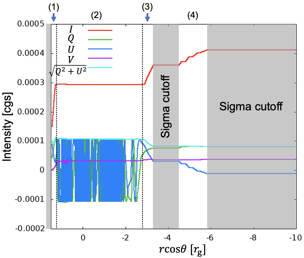
Further, we pick up a pixel pointed by a white “x” in the left image of Fig. B2, and show the radiative transfer plots along the light path (shown in the central and right panel of of Fig. B2) in Fig. B3. The pixel is located in the brightest region in the total intensity image, and around a “cross-section” between the photon ring and the tail-like jet feature.
We can follow up the radiative transfer plot lines of Stokes parameters in Fig. B3 by four steps, referring the radiative coefficients in Fig. B1, as follows:
- (1)
the synchrotron emission occurs in the jet-edge in the north () side simultaneously with the Faraday rotation and conversion processes. Combination of these effects leads to increase of both LP () and CP (), in addition to the total intensity (), as we also introduced in Tsunetoe et al. 2020a.
- (2)
Entering the disk region around the equatorial plane, Faraday rotation becomes dominant. Thus, the LP vector is drastically rotated, giving rise to rapid oscillations of and .
- (3)
In the jet-edge in the south () side, the emission arises again. While the total intensity increases, the rotated LP vector are partly canceled out with the new emission component. The CP does not change significantly due to weak Faraday conversion, because the light is now passing through the outer or downstream region relatively to the prior northern jet-edge. After leaving this region, the light enters the sigma cutoff region in the southern funnel region.
- (4)
There is a low- region in the funnel distributed in a spiral shape in the three-dimensional fluid model. This feature can be seen, for example, as a “hump”-like feature along the jet-edge around in the left panel of Fig. B1. Here, the total intensity increases and the LP is overwritten in similar way to (3) in the south jet-edge, since the synchrotron emission occurs again.
As a result, we obtain the total intensity increased in the inner jet-edges and the downstream spiral low- component, which can be seen as the photon ring and the tail-like jet on the image. Further, the obtained LP vector consists of the rotated components from the north (counter-side) jet-edge and the overwriting emission from the south (approaching) jet-edge. Finally, the obtained CP is originated from those increased in the north (counter-side) jet-edge. Therefore, the LP map is dominated by the contributions from the approaching jet while the CP image by those from the counter-side jet, after the observational beam convolution. In this way, we demonstrate that the scenario pictured in Fig. 6 actually occurs in the radiative transfer calculation.

Appendix C Correlation maps in polar coordinates
In Fig. C1, we show three maps of auto- and cross- correlation functions , , and for polar coordinates on the images at 230GHz, defined by Eq. 6. The positive (negative) corresponds to counterclockwise (clockwise) direction on the images. The maps have a period of in the direction, so that they have same values in the top () and bottom ().
The auto correlation for the total intensity, has a peak at by definition. In the radial, - direction, two cross-correlations and have little deviations from the center, reflecting the fact that most of the total, LP and CP intensities are distributed on the common ring. Meanwhile, () gives a peak at positive (negative) region in the azimuthal, - direction. Now the total intensity image is brighter in the left side of the asymmetric ring feature, so this results quantify the tendency that the LP (CP) intensities are distributed in the lower-left (upper-left) of the common ring.

Appendix D Vertical peak shifts of and for the cases seeing from behind
In Fig. D1, We show the vertical peak shifts of the cross-correlation functions for different parameters, as in Fig. 7, but for the azimuthal angle position of the camera , which corresponds to the observer in the opposite side with respect to the jet (z-) axis.

Appendix E Vertical and horizontal profiles of cross-correlation functions and for different model parameters
In the text, we showed only the vertical peak shifts of the correlation functions at the higher and lower frequencies except 230 and 86 GHz, and for various model parameters except a high accretion model with . Here, we show the vertical (-) and horizontal (-) profiles of the correlation functions, in Figs.E1 to E6.


Appendix F A scatter diagram with histogram of and vertical peaks for sixteen images
In Fig. F1, we show a scatter diagram with histogram of the peak shifts of and on the sixteen images introduced in subsection IV.7, where 13 out of 16 images show the LP-CP separation (in the yellow-marked region in the diagram). It also shows that 9 of 16 images give peak shifts larger than , while 5 images yield peak shift larger than .

References
- Abramowski et al. (2012) Abramowski, A., Acero, F., Aharonian, F., et al. 2012, ApJ, 746, 151, doi: 10.1088/0004-637X/746/2/151
- Aharonian et al. (2006) Aharonian, F., Akhperjanian, A. G., Bazer-Bachi, A. R., et al. 2006, Science, 314, 1424, doi: 10.1126/science.1134408
- Akiyama et al. (2015) Akiyama, K., Lu, R.-S., Fish, V. L., et al. 2015, ApJ, 807, 150, doi: 10.1088/0004-637X/807/2/150
- Akiyama et al. (2017a) Akiyama, K., Kuramochi, K., Ikeda, S., et al. 2017a, ApJ, 838, 1, doi: 10.3847/1538-4357/aa6305
- Akiyama et al. (2017b) Akiyama, K., Ikeda, S., Pleau, M., et al. 2017b, AJ, 153, 159, doi: 10.3847/1538-3881/aa6302
- Algaba et al. (2016) Algaba, J. C., Asada, K., & Nakamura, M. 2016, ApJ, 823, 86, doi: 10.3847/0004-637X/823/2/86
- Algaba et al. (2021) Algaba, J. C., Anczarski, J., Asada, K., et al. 2021, arXiv e-prints, arXiv:2104.06855. https://arxiv.org/abs/2104.06855
- Anantua et al. (2020) Anantua, R., Emami, R., Loeb, A., & Chael, A. 2020, ApJ, 896, 30, doi: 10.3847/1538-4357/ab9103
- Asada & Nakamura (2012) Asada, K., & Nakamura, M. 2012, ApJ, 745, L28, doi: 10.1088/2041-8205/745/2/L28
- Asada et al. (2014) Asada, K., Nakamura, M., Doi, A., Nagai, H., & Inoue, M. 2014, ApJ, 781, L2, doi: 10.1088/2041-8205/781/1/L2
- Balbus & Hawley (1991) Balbus, S. A., & Hawley, J. F. 1991, ApJ, 376, 214, doi: 10.1086/170270
- Biretta et al. (1995) Biretta, J. A., Zhou, F., & Owen, F. N. 1995, ApJ, 447, 582, doi: 10.1086/175901
- Blandford & Begelman (1999) Blandford, R. D., & Begelman, M. C. 1999, MNRAS, 303, L1, doi: 10.1046/j.1365-8711.1999.02358.x
- Blandford & Königl (1979) Blandford, R. D., & Königl, A. 1979, ApJ, 232, 34, doi: 10.1086/157262
- Blandford & Payne (1982) Blandford, R. D., & Payne, D. G. 1982, MNRAS, 199, 883, doi: 10.1093/mnras/199.4.883
- Blandford & Znajek (1977) Blandford, R. D., & Znajek, R. L. 1977, MNRAS, 179, 433, doi: 10.1093/mnras/179.3.433
- Bridle & Perley (1984) Bridle, A. H., & Perley, R. A. 1984, ARA&A, 22, 319, doi: 10.1146/annurev.aa.22.090184.001535
- Broderick & Loeb (2009) Broderick, A. E., & Loeb, A. 2009, ApJ, 697, 1164, doi: 10.1088/0004-637X/697/2/1164
- Bronzwaer et al. (2020) Bronzwaer, T., Younsi, Z., Davelaar, J., & Falcke, H. 2020, A&A, 641, A126, doi: 10.1051/0004-6361/202038573
- Chael et al. (2019) Chael, A., Narayan, R., & Johnson, M. D. 2019, MNRAS, 486, 2873, doi: 10.1093/mnras/stz988
- Chael et al. (2016) Chael, A. A., Johnson, M. D., Narayan, R., et al. 2016, ApJ, 829, 11, doi: 10.3847/0004-637X/829/1/11
- Davelaar et al. (2019) Davelaar, J., Olivares, H., Porth, O., et al. 2019, A&A, 632, A2, doi: 10.1051/0004-6361/201936150
- Dexter (2016) Dexter, J. 2016, MNRAS, 462, 115, doi: 10.1093/mnras/stw1526
- Dexter et al. (2012) Dexter, J., McKinney, J. C., & Agol, E. 2012, MNRAS, 421, 1517, doi: 10.1111/j.1365-2966.2012.20409.x
- Dexter et al. (2020) Dexter, J., Jiménez-Rosales, A., Ressler, S. M., et al. 2020, MNRAS, 494, 4168, doi: 10.1093/mnras/staa922
- Di Matteo et al. (2003) Di Matteo, T., Allen, S. W., Fabian, A. C., Wilson, A. S., & Young, A. J. 2003, ApJ, 582, 133, doi: 10.1086/344504
- Doeleman et al. (2012) Doeleman, S. S., Fish, V. L., Schenck, D. E., et al. 2012, Science, 338, 355, doi: 10.1126/science.1224768
- Emami et al. (2021) Emami, R., Anantua, R., Chael, A. A., & Loeb, A. 2021, arXiv e-prints, arXiv:2101.05327. https://arxiv.org/abs/2101.05327
- Enßlin (2003) Enßlin, T. A. 2003, A&A, 401, 499, doi: 10.1051/0004-6361:20030162
- Event Horizon Telescope Collaboration et al. (2019a) Event Horizon Telescope Collaboration, Akiyama, K., Alberdi, A., et al. 2019a, ApJ, 875, L1, doi: 10.3847/2041-8213/ab0ec7
- Event Horizon Telescope Collaboration et al. (2019b) —. 2019b, ApJ, 875, L5, doi: 10.3847/2041-8213/ab0f43
- Event Horizon Telescope Collaboration et al. (2019c) —. 2019c, ApJ, 875, L4, doi: 10.3847/2041-8213/ab0e85
- Event Horizon Telescope Collaboration et al. (2021a) Event Horizon Telescope Collaboration, Akiyama, K., Algaba, J. C., et al. 2021a, ApJ, 910, L12, doi: 10.3847/2041-8213/abe71d
- Event Horizon Telescope Collaboration et al. (2021b) —. 2021b, ApJ, 910, L13, doi: 10.3847/2041-8213/abe4de
- Fishbone & Moncrief (1976) Fishbone, L. G., & Moncrief, V. 1976, ApJ, 207, 962, doi: 10.1086/154565
- Ford et al. (1994) Ford, H. C., Harms, R. J., Tsvetanov, Z. I., et al. 1994, ApJ, 435, L27, doi: 10.1086/187586
- Gabuzda et al. (2008) Gabuzda, D. C., Vitrishchak, V. M., Mahmud, M., & O’Sullivan, S. P. 2008, MNRAS, 384, 1003, doi: 10.1111/j.1365-2966.2007.12773.x
- Gammie (2004) Gammie, C. F. 2004, ApJ, 614, 309, doi: 10.1086/423443
- Gammie et al. (2003) Gammie, C. F., McKinney, J. C., & Tóth, G. 2003, ApJ, 589, 444, doi: 10.1086/374594
- Gebhardt et al. (2011) Gebhardt, K., Adams, J., Richstone, D., et al. 2011, ApJ, 729, 119, doi: 10.1088/0004-637X/729/2/119
- Goddi et al. (2021) Goddi, C., Marti-Vidal, I., Messias, H., et al. 2021, arXiv e-prints, arXiv:2105.02272. https://arxiv.org/abs/2105.02272
- Gold et al. (2017) Gold, R., McKinney, J. C., Johnson, M. D., & Doeleman, S. S. 2017, ApJ, 837, 180, doi: 10.3847/1538-4357/aa6193
- Hada et al. (2011) Hada, K., Doi, A., Kino, M., et al. 2011, Nature, 477, 185, doi: 10.1038/nature10387
- Hada et al. (2013) Hada, K., Kino, M., Doi, A., et al. 2013, ApJ, 775, 70, doi: 10.1088/0004-637X/775/1/70
- Hada et al. (2016) —. 2016, ApJ, 817, 131, doi: 10.3847/0004-637X/817/2/131
- Hawley et al. (2011) Hawley, J. F., Guan, X., & Krolik, J. H. 2011, ApJ, 738, 84, doi: 10.1088/0004-637X/738/1/84
- Ho et al. (1997) Ho, L. C., Filippenko, A. V., & Sargent, W. L. W. 1997, ApJS, 112, 315, doi: 10.1086/313041
- Hodge (1982) Hodge, P. E. 1982, ApJ, 263, 595, doi: 10.1086/160530
- Homan et al. (2009) Homan, D. C., Lister, M. L., Aller, H. D., Aller, M. F., & Wardle, J. F. C. 2009, ApJ, 696, 328, doi: 10.1088/0004-637X/696/1/328
- Howes (2010) Howes, G. G. 2010, MNRAS, 409, L104, doi: 10.1111/j.1745-3933.2010.00958.x
- Jeter et al. (2020) Jeter, B., Broderick, A. E., & Gold, R. 2020, MNRAS, 493, 5606, doi: 10.1093/mnras/staa679
- Jiménez-Rosales & Dexter (2018) Jiménez-Rosales, A., & Dexter, J. 2018, MNRAS, 478, 1875, doi: 10.1093/mnras/sty1210
- Johnson et al. (2014) Johnson, M. D., Fish, V. L., Doeleman, S. S., et al. 2014, ApJ, 794, 150, doi: 10.1088/0004-637X/794/2/150
- Johnson et al. (2015) —. 2015, Science, 350, 1242, doi: 10.1126/science.aac7087
- Jones (1988) Jones, T. W. 1988, ApJ, 332, 678, doi: 10.1086/166685
- Jones & O’Dell (1977) Jones, T. W., & O’Dell, S. L. 1977, ApJ, 214, 522, doi: 10.1086/155278
- Junor et al. (1999) Junor, W., Biretta, J. A., & Livio, M. 1999, Nature, 401, 891, doi: 10.1038/44780
- Kato et al. (2008) Kato, S., Fukue, J., & Mineshige, S. 2008, Black-Hole Accretion Disks — Towards a New Paradigm —
- Kawashima et al. (2019) Kawashima, T., Kino, M., & Akiyama, K. 2019, ApJ, 878, 27, doi: 10.3847/1538-4357/ab19c0
- Kawashima et al. (2021a) Kawashima, T., Ohsuga, K., & Takahashi, H. R. 2021a, arXiv e-prints, arXiv:2108.05131. https://arxiv.org/abs/2108.05131
- Kawashima et al. (2021b) Kawashima, T., Toma, K., Kino, M., et al. 2021b, ApJ, 909, 168, doi: 10.3847/1538-4357/abd5bb
- Kawazura et al. (2019) Kawazura, Y., Barnes, M., & Schekochihin, A. A. 2019, Proceedings of the National Academy of Science, 116, 771, doi: 10.1073/pnas.1812491116
- Kim et al. (2018) Kim, J. Y., Krichbaum, T. P., Lu, R. S., et al. 2018, A&A, 616, A188, doi: 10.1051/0004-6361/201832921
- Kino et al. (2014) Kino, M., Takahara, F., Hada, K., & Doi, A. 2014, ApJ, 786, 5, doi: 10.1088/0004-637X/786/1/5
- Koide et al. (1999) Koide, S., Shibata, K., & Kudoh, T. 1999, ApJ, 522, 727, doi: 10.1086/307667
- Komissarov (2005) Komissarov, S. S. 2005, MNRAS, 359, 801, doi: 10.1111/j.1365-2966.2005.08974.x
- Kovalev et al. (2007) Kovalev, Y. Y., Lister, M. L., Homan, D. C., & Kellermann, K. I. 2007, ApJ, 668, L27, doi: 10.1086/522603
- Kravchenko et al. (2020) Kravchenko, E., Giroletti, M., Hada, K., et al. 2020, A&A, 637, L6, doi: 10.1051/0004-6361/201937315
- Kuo et al. (2014) Kuo, C. Y., Asada, K., Rao, R., et al. 2014, ApJ, 783, L33, doi: 10.1088/2041-8205/783/2/L33
- Legg & Westfold (1968) Legg, M. P. C., & Westfold, K. C. 1968, ApJ, 154, 499, doi: 10.1086/149777
- Lu et al. (2014) Lu, R.-S., Broderick, A. E., Baron, F., et al. 2014, ApJ, 788, 120, doi: 10.1088/0004-637X/788/2/120
- Ly et al. (2007) Ly, C., Walker, R. C., & Junor, W. 2007, ApJ, 660, 200, doi: 10.1086/512846
- Lynden-Bell (1969) Lynden-Bell, D. 1969, Nature, 223, 690, doi: 10.1038/223690a0
- Macchetto et al. (1997) Macchetto, F., Marconi, A., Axon, D. J., et al. 1997, ApJ, 489, 579, doi: 10.1086/304823
- Mahadevan et al. (1996) Mahadevan, R., Narayan, R., & Yi, I. 1996, ApJ, 465, 327, doi: 10.1086/177422
- Marshall et al. (2002) Marshall, H. L., Miller, B. P., Davis, D. S., et al. 2002, ApJ, 564, 683, doi: 10.1086/324396
- McKinney et al. (2012) McKinney, J. C., Tchekhovskoy, A., & Blandford, R. D. 2012, MNRAS, 423, 3083, doi: 10.1111/j.1365-2966.2012.21074.x
- Mei et al. (2007) Mei, S., Blakeslee, J. P., Côté, P., et al. 2007, ApJ, 655, 144, doi: 10.1086/509598
- Mertens et al. (2016) Mertens, F., Lobanov, A. P., Walker, R. C., & Hardee, P. E. 2016, A&A, 595, A54, doi: 10.1051/0004-6361/201628829
- Mizuno et al. (2021) Mizuno, Y., Fromm, C. M., Younsi, Z., et al. 2021, arXiv e-prints, arXiv:2106.09272. https://arxiv.org/abs/2106.09272
- Mościbrodzka et al. (2017) Mościbrodzka, M., Dexter, J., Davelaar, J., & Falcke, H. 2017, MNRAS, 468, 2214, doi: 10.1093/mnras/stx587
- Mościbrodzka & Falcke (2013) Mościbrodzka, M., & Falcke, H. 2013, A&A, 559, L3, doi: 10.1051/0004-6361/201322692
- Mościbrodzka et al. (2016) Mościbrodzka, M., Falcke, H., & Shiokawa, H. 2016, A&A, 586, A38, doi: 10.1051/0004-6361/201526630
- Moscibrodzka et al. (2021) Moscibrodzka, M., Janiuk, A., & De Laurentis, M. 2021, arXiv e-prints, arXiv:2103.00267. https://arxiv.org/abs/2103.00267
- Nakamura & Asada (2013) Nakamura, M., & Asada, K. 2013, ApJ, 775, 118, doi: 10.1088/0004-637X/775/2/118
- Nakamura et al. (2018) Nakamura, M., Asada, K., Hada, K., et al. 2018, ApJ, 868, 146, doi: 10.3847/1538-4357/aaeb2d
- Narayan et al. (2003) Narayan, R., Igumenshchev, I. V., & Abramowicz, M. A. 2003, PASJ, 55, L69, doi: 10.1093/pasj/55.6.L69
- Narayan et al. (2012) Narayan, R., SÄ dowski, A., Penna, R. F., & Kulkarni, A. K. 2012, MNRAS, 426, 3241, doi: 10.1111/j.1365-2966.2012.22002.x
- Narayan & Yi (1995) Narayan, R., & Yi, I. 1995, ApJ, 452, 710, doi: 10.1086/176343
- Noble et al. (2006) Noble, S. C., Gammie, C. F., McKinney, J. C., & Del Zanna, L. 2006, ApJ, 641, 626, doi: 10.1086/500349
- Owen et al. (1990) Owen, F. N., Eilek, J. A., & Keel, W. C. 1990, ApJ, 362, 449, doi: 10.1086/169282
- Owen et al. (1989) Owen, F. N., Hardee, P. E., & Cornwell, T. J. 1989, ApJ, 340, 698, doi: 10.1086/167430
- Park et al. (2019a) Park, J., Hada, K., Kino, M., et al. 2019a, ApJ, 871, 257, doi: 10.3847/1538-4357/aaf9a9
- Park et al. (2019b) —. 2019b, ApJ, 887, 147, doi: 10.3847/1538-4357/ab5584
- Rees (1984) Rees, M. J. 1984, ARA&A, 22, 471, doi: 10.1146/annurev.aa.22.090184.002351
- Ricarte et al. (2020) Ricarte, A., Prather, B. S., Wong, G. N., et al. 2020, MNRAS, 498, 5468, doi: 10.1093/mnras/staa2692
- Ricarte et al. (2021) Ricarte, A., Qiu, R., & Narayan, R. 2021, MNRAS, doi: 10.1093/mnras/stab1289
- Ryan et al. (2018) Ryan, B. R., Ressler, S. M., Dolence, J. C., Gammie, C., & Quataert, E. 2018, ApJ, 864, 126, doi: 10.3847/1538-4357/aad73a
- Sädowski et al. (2013) Sädowski, A., Narayan, R., Penna, R., & Zhu, Y. 2013, MNRAS, 436, 3856, doi: 10.1093/mnras/stt1881
- Sanders et al. (1989) Sanders, D. B., Phinney, E. S., Neugebauer, G., Soifer, B. T., & Matthews, K. 1989, ApJ, 347, 29, doi: 10.1086/168094
- Sano et al. (2004) Sano, T., Inutsuka, S.-i., Turner, N. J., & Stone, J. M. 2004, ApJ, 605, 321, doi: 10.1086/382184
- Shcherbakov (2008) Shcherbakov, R. V. 2008, ApJ, 688, 695, doi: 10.1086/592326
- Takahashi et al. (2018) Takahashi, H. R., Mineshige, S., & Ohsuga, K. 2018, ApJ, 853, 45, doi: 10.3847/1538-4357/aaa082
- Takahashi et al. (2016) Takahashi, H. R., Ohsuga, K., Kawashima, T., & Sekiguchi, Y. 2016, ApJ, 826, 23, doi: 10.3847/0004-637X/826/1/23
- Tchekhovskoy et al. (2011) Tchekhovskoy, A., Narayan, R., & McKinney, J. C. 2011, MNRAS, 418, L79, doi: 10.1111/j.1745-3933.2011.01147.x
- Tsunetoe et al. (2020a) Tsunetoe, Y., Mineshige, S., Ohsuga, K., Kawashima, T., & Akiyama, K. 2020a, PASJ, 72, 32, doi: 10.1093/pasj/psaa008
- Tsunetoe et al. (2020b) —. 2020b, arXiv e-prints, arXiv:2012.05243. https://arxiv.org/abs/2012.05243
- Walker et al. (2018) Walker, R. C., Hardee, P. E., Davies, F. B., Ly, C., & Junor, W. 2018, ApJ, 855, 128, doi: 10.3847/1538-4357/aaafcc
- Wardle & Homan (2003) Wardle, J. F. C., & Homan, D. C. 2003, Ap&SS, 288, 143, doi: 10.1023/B:ASTR.0000005001.80514.0c
- Yuan & Narayan (2014) Yuan, F., & Narayan, R. 2014, ARA&A, 52, 529, doi: 10.1146/annurev-astro-082812-141003
- Zavala & Taylor (2002) Zavala, R. T., & Taylor, G. B. 2002, ApJ, 566, L9, doi: 10.1086/339441
- Zavala & Taylor (2003) —. 2003, ApJ, 589, 126, doi: 10.1086/374619
- Zavala & Taylor (2004) —. 2004, ApJ, 612, 749, doi: 10.1086/422741
- Zensus (1997) Zensus, J. A. 1997, ARA&A, 35, 607, doi: 10.1146/annurev.astro.35.1.607