Energy exchange between relativistic fluids: the polytropic case
Abstract
We present a simple, analytic and straightforward method to elucidate the effects produced by polytropic fluids on any other gravitational source, no matter its nature, for static and spherically symmetric spacetimes. As a direct application, we study the interaction between polytropes and perfect fluids coexisting inside a self-gravitating stellar object.
I Introduction
The study of self-gravitating systems is of great importance in the context of general relativity. In particular, elucidating what happens inside compact stellar distributions is extremely important, especially if we want to gain a good understanding of gravitational collapse. Presumably, the interior of a stellar structure is a complex physical system, formed by fluids of different natures, which surely interact with each other in a non-trivial way. Although it is true that we can always group fluids of different nature into a single energy-momentum tensor , namely,
| (1) |
as indeed it is required by Einstein’s field equations, it is no less true that an oversimplification of these systems could jeopardize an adequate description of them. A clear example of this occurs when we consider complex stellar distributions (being electrically charged, with dissipative effects, anisotropic, etc.) and impose a fairly simple equation of state to describe the system as a whole. This could mean an oversimplification whose main motivation is far from being physical: a reduction of the degrees of freedom of the system that makes it more manageable. It is true that in many cases this strategy produces great results, such as exact and physically reasonable solutions, but perhaps we are paying a high price without being aware of it, such as a rather idealized description of a system whose physical nature is intrinsically complex.
Regarding the above, it would be very useful to see how relevant is the role that each fluid, represented by their respective energy-momentum tensor in (1), plays on a self-gravitating system, as well as how these gravitational sources interact with each other. This would allow, for instance, detecting which source dominates over the others, and consequently rule out any equation of state incompatible with the dominant source. Conceptually, achieving this in general relativity should be extremely difficult, given the nonlinear nature of the theory. However, since the Gravitational Decoupling approach (GD) Ovalle 2017; Ovalle 2019 is precisely designed for coupling/decoupling gravitational sources in general relativity, we will see that, indeed, it is possible to elucidate the role played by each gravitational source, without resorting to any numerical protocol or perturbation scheme, as explained in the next paragraph.
In particular, if in Eq. (1) we consider two arbitrary sources , then the contracted Bianchi identities yields . This has two possible solutions, namely,
The first solution indicates that each source is covariantly conserved, and therefore the interaction between them is purely gravitational. The second option, more interesting and much more realistic,11 1 If both fluids coexist in a certain region of spacetime, as in fact occurs within a self-gravitating object. indicates an exchange of energy between these sources that, in principle, would be impossible to quantify or at least describe in some detail. The reason for this is that the Bianchi identities do not introduce additional information beyond Einstein’s equations. They are identities, and therefore are trivially satisfied. However, the GD is precisely the scheme that circumvents the intrinsic triviality of Bianchi identities, and it is what allows to elucidate, in detail, the interaction between both gravitational sources [see further Eq. (31)].
In particular, and motivated by the interest that they have generated in recent years, in this article we will choose a polytrope as one of the gravitational sources to determine its effects on any other generic fluid, regardless of its nature.
The paper is organised as follows: in Section II, we first review the fundamentals of the GD approach to a spherically symmetric system containing two generic sources; in Section III, we choose a polytropic fluid to study its effects on a generic gravitational source, and we introduce a systematic and direct procedure to elucidate these effects; in Section IV, we implement the strategy developed in Section III for the case of a perfect fluid; finally, we summarize our conclusions in Section V.
II Gravitational Decoupling
In this Section, we briefly review the GD for spherically symmetric gravitational systems described in detail in Ref. Ovalle 2019. For the axially symmetric case, see Ref. Contreras et al. 2021. The gravitational decoupling approach and its simplest version Ovalle 2017, based in the Minimal Geometric Deformation (MGD) Ovalle and Casadio 2020; da Rocha 2017a; da Rocha 2017b; Fernandes-Silva and da Rocha 2018; Casadio et al. 2018; Fernandes-Silva et al. 2018; Contreras and Bargueño 2018a; Contreras 2018; Contreras and Bargueño 2018b; Panotopoulos and Rincón 2018; Da Rocha and Tomaz 2019; Las Heras and León 2019; Rincón et al. 2019; da Rocha 2020a; Contreras et al. 2020; Arias et al. 2020; da Rocha 2020b; Tello-Ortiz et al. 2020; da Rocha and Tomaz 2020; Meert and da Rocha 2021; Tello-Ortiz et al. 2021; Maurya and Nag 2021; Azmat and Zubair 2021a; Maurya et al. 2022, are attractive for many reasons (for an incomplete list of references, see Ovalle et al. 2018a; Gabbanelli et al. 2018; Heras and Leon 2018; Estrada and Tello-Ortiz 2018; Sharif and Sadiq 2018a; Sharif and Sadiq 2018b; Morales and Tello-Ortiz 2018; Estrada and Prado 2019; Sharif and Saba 2018; Ovalle et al. 2018b; Contreras 2019; Contreras et al. 2019; Contreras and Bargueño 2019; Gabbanelli et al. 2019; Estrada 2019; Ovalle et al. 2019; Ovalle et al. 2019; Hensh and Stuchlík 2019; Linares Cedeño and Contreras 2020; Torres-Sánchez and Contreras 2019; Casadio et al. 2019; Singh et al. 2019; Maurya 2019; Sharif and Waseem 2019; Singh et al. 2019; Abellan et al. 2020; Sharif and Ama-Tul-Mughani 2020; Tello-Ortiz 2020; Maurya 2020; Rincón et al. 2020; Sharif and Majid 2020; Maurya et al. 2020a; Zubair and Azmat 2020; Sharif and Saba 2020; Ovalle et al. 2021a; Estrada and Prado 2020; Maurya et al. 2020b; Maurya et al. 2021a; Azmat and Zubair 2021b; Islam and Ghosh 2021; Afrin et al. 2021; Ovalle et al. 2021b; Ama-Tul-Mughani et al. 2021; Sharif and Aslam 2021; da Rocha 2021; Maurya et al. 2021b; Carrasco-Hidalgo and Contreras 2021; Sultana 2021; da Rocha 2022; Maurya and Nag 2022; Omwoyo et al. 2021; Afrin and Ghosh 2022; Meert and da Rocha 2022. Among them we can mention i) the coupling of gravitational sources, which allows for extending known solutions of the Einstein field equations into more complex domains; ii) the decoupling of gravitational sources, which is used to systematically reduce (decouple) a complex energy-momentum tensor into simpler components; iii) to find solutions in gravitational theories beyond Einstein’s; iv) to generate rotating hairy black hole solutions, among many others applications.
Let us consider the Einstein field equations 22 2 We use units with and , where is Newton’s constant.
| (2) |
with a total energy-momentum tensor given by,
| (3) |
where is usually associated with some already known solution, whereas may contain new fields or even be related with a new gravitational sector not described by general relativity. As a consequence of Bianchi identity, the total source must be covariantly conserved,
| (4) |
For spherically symmetric and static systems, we can write the metric as
| (5) |
where and are functions of the areal radius only and . The Einstein equations (2) then read
| (6) | |||||
| (7) | |||||
| (8) |
where and due to the spherical symmetry. By simple inspection, we can identify in Eqs. (6)-(8) an effective density
| (9) |
an effective radial pressure
| (10) |
and an effective tangential pressure
| (11) |
where clearly we have
| (12) | |||
| (13) |
In general, the anisotropy
| (14) |
does not vanish and the system of Eqs. (6)-(8) may be treated as an anisotropic fluid.
We next consider a solution to the Eqs. (2) for the seed source alone, that is,
| (15) |
which we write as
| (16) |
where
| (17) |
is the standard general relativity expression containing the Misner-Sharp mass function . The consequences of adding the source can be seen in the geometric deformation of the metric (16), namely33 3 usually we write and , with a parameter introduced to keep track of these deformations. Here we dispense with it for simplicity.
| (18) | |||||
| (19) |
where and are respectively the geometric deformations for the radial and temporal metric components. We emphasize that the expressions in Eqs. (18) and (19) are not a coordinate transformation. They just represent the change in the spacetime geometry (16) generated by a physical source with energy-momentum tensor .
By means of Eqs. (18) and (19), the Einstein equations (6)-(8) are separated in two sets: A) one is given by the standard Einstein field equations with the energy-momentum tensor , that is
| (20) | |||
| (21) | |||
| (22) |
which is assumed to be solved by the metric (16); B) the second set contains the source and reads
| (23) | |||||
| (24) | |||||
| (25) | |||||
where
| (26) | |||||
| (27) |
Of course the tensor vanishes when the deformations vanish (). We see that for the particular case , Eqs. (23)-(25) reduce to the simpler “quasi-Einstein” system of the MGD of Ref. Ovalle 2017, in which is only determined by and the undeformed metric (16). Also, notice that the set (23)-(25) contains , and therefore is not independent of (20)-(22). This of course makes sense since both systems represent a simplified version of a more complex whole, described by Eqs. (6)-(8).
Now let us see the conservation equation (4), which reads
| (28) |
The bracket represents the divergence of computed with the covariant derivative for the metric (16), and is a linear combination of the Einstein field equations (20)-(22). Since the Einstein tensor for the metric (16) satisfies its respective Bianchi identity, the momentum tensor is conserved in this geometry,
| (29) |
Notice that
| (30) |
where the divergence in the left-hand side is calculated with the deformed metric in Eq. (5). Finally, Eq. (II) becomes
| (31) |
which is also a linear combination of the “quasi-Einstein” field equations (23)-(25) for the source . We therefore conclude that the two sources and can be successfully decoupled by means of the GD. This result is particularly remarkable since it is exact, without requiring any perturbative expansion in or Ovalle and Casadio 2020.
Finally, in order to be as self-contained as possible, and to clarify the reader any potential confusion about what we developed between Eqs. (2)-(31), we next describe the intrinsic relationship between gravitational decoupling and energy exchange for coupled/decoupled relativistic fluids.
- 1.
- 2.
- 3.
The new spacetime geometry , associated with the total source , satisfies Einstein’s equations (6)-(8) if and only if the source and its geometric functions satisfy the equation of motions (23)-(25).
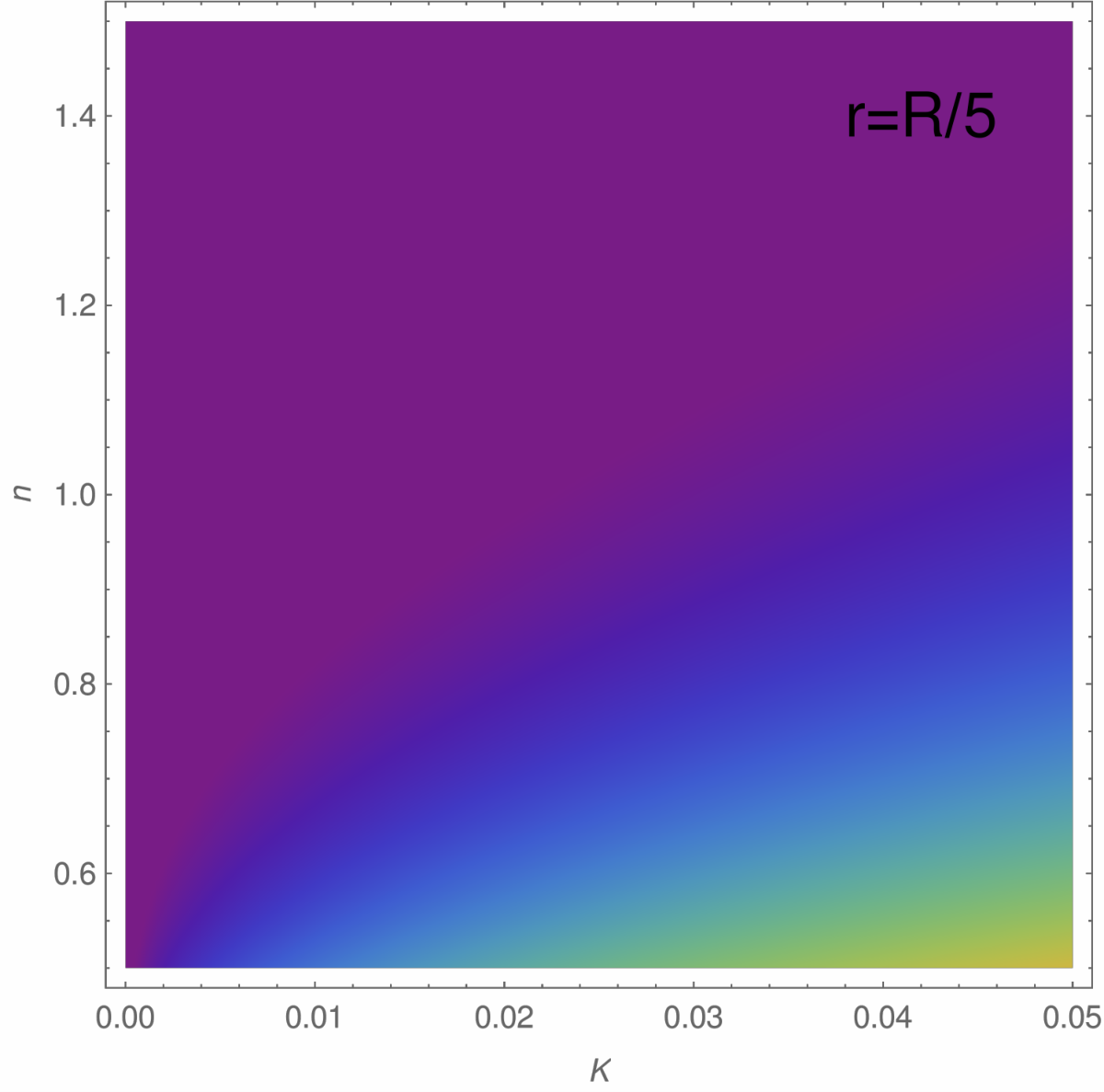
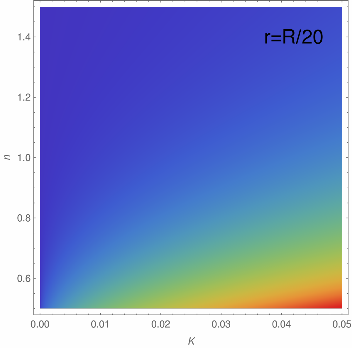
Figure 1: Radial pressure for two inner layers. - 4.
The complete process describes previously cannot be arbitrary and, in fact, is subject to the fulfillment of Bianchi identities, which implies that is covariantly conserved, i.e., . This yields the expression in Eq. (31), showing an energy exchange between the relativistic fluids .
We want to conclude by emphasizing two aspects that we must always keep in mind:
- •
The GD approach is an exact scheme.
- •
Regardless of the origin of (as we have already mentioned, it can even represent a new gravitational sector), all our analysis is confined to the context of general relativity.
- •
- •
II.1 Matching conditions at the surface
The interior () of the self-gravitating system of radius () is described by the metric (5), which we can conveniently write as
| (32) |
where the interior mass function is given by
| (33) |
with the Misner-Sharp mass given in Eq. (17) and the geometric deformation in Eq. (19). On the other hand, the exterior () space-time will be described by the Schwarzschild metric
| (34) |
To have a smooth continuity, the metrics in Eqs. (32) and (34) must satisfy the Israel-Darmois matching conditions at the star surface defined by . In particular, the continuity of the metric across implies
| (35) |
and
| (36) |
Likewise, the second fundamental form yields
| (37) |
where is the unit radial vector normal to a surface of constant . Hence, using Einstein equations in Eq. (37), we have
| (38) |
This matching condition takes the final form
| (39) |
where and . The condition (39) can be written as
| (40) |
where . Eqs. (35), (36) and (40) are the necessary and sufficient conditions for matching the interior GD metric (32) with the outer Schwarzschild metric (34).
III Polytropic equation of state
So far, all our analysis has been generic, without specifying the sources that compose our system. Of all the possible gravitational sources, we will choose one of particular importance, which has been extensively investigated. We refer to a polytropic fluid, which in our case will be represented by the tensor . Hence, following our previous analysis, we will see how to elucidate the effects of a polytrope on another generic source describe by Einstein’s equations (20)-(22).
If the tensor represents an isotropic polytrope, it satisfies the equation of state
| (41) |
However, in our case we will require that only the radial pressure satisfies the equation of state (41), allowing the tangential component to evolve independently. Hence,
| (42) |
with , where is the polytropic index and denotes a parameter which contains the temperature implicitly and is governed by the thermal characteristics of a given polytrope. (For all details regarding basic concepts of polytropes, see for instance Ref. Horedt 2004, also see references Refs. Herrera and Barreto 2013; Stuchlík et al. 2016; Stuchlik 2000; Novotný et al. 2017; Stuchlík et al. 2017; Posada et al. 2020).).
Let us start by using Eqs. (23) and (24) in the expression (42), which yields a first order non-linear differential equation for the deformation ,
| (43) |
Therefore, given a seed solution to Einstein equations (20)-(22), we end with a non-linear differential expression in Eq. (43) to determinate the deformations . Hence, we need to prescribe additional information. In any case, we must be careful in keeping the physical acceptability of the seed solution , which is not a trivial issue. In this respect, and in order to ensure the coupling condition in Eq. (40), we impose the so-called mimic constraint for the pressure, namely,
| (44) |
The simplest expression for satisfying the constraint (44) is given by
| (45) |
where is a characteristic function for each polytrope. The simplest form for consistent with the polytropic equation of state (42) and with the condition
| (46) |
is given by
| (47) |
Hence, the expression (45) becomes
| (48) |
Expressions in Eqs. (43) and (48) now are written as
| (49) | |||
We see that for a given seed solution to Einstein equations (20)-(22), we can determinate its deformation produced for any polytrope by Eqs. (49) and (III).
A condition other than (44), also useful to ensure a physically acceptable solution, is to impose the so-called mimic constraint for the pressure, i.e,
| (51) |
Hence, following the same reasoning as Eqs. (45)-(47), we have
| (52) |
which yields,
| (53) | |||
In short, our approach allows to determinate the effects of politropes on any generic fluid, represented by and satisfying Einstein equations (20)-(22), no matter its nature.
Note that if we impose the constraint (45), we are faced with solving the nonlinear differential equation (49) to determine . Instead, if we impose the condition (52), we will need to solve the linear differential equation (53) to find . Everything seems to indicate that it is more convenient to impose the constraint (52). However, using the condition (45) has a quite useful advantage: the coupling problem on the surface, which could be non-trivial in some cases, is greatly reduced.
Finally, we see that a critical characteristic of the interaction between both fluids, such as the exchange of energy-momentum between them, is easily elucidated by [see Eq. (31)]
| (55) |
which we can write in terms of pure geometric functions as [see Eqs. (20)-(22)]
| (56) |
From the expression (55) we can see that yields . This indicates , according to the conservation equation (31), which means that the polytrope is giving energy to the environment. The opposite happens when .


III.0.1 Strategy
We can now detail our scheme to elucidate the effects of the polytrope on any other generic fluid , no matter its nature (isotropic, charged, scalar field, etc.):
- 1.
- 2.
Consider a polytropic fluid, characterized by the constant and index in the equation of state (42).
- 3.
- 4.
- 5.
- 6.
We want to emphasize that the previous scheme allows us to study the coexistence of a polytropic fluid with any other, and elucidate the effects of the former on the latter, by a systematic and direct way. Next we will consider a perfect fluid as a seed solution to elucidate the consequences of polytrope on this gravitational sources.
IV Coexistence of polytropes
and perfect fluids
In particular, we can simply choose a known solution with physical relevance, like the well-known Tolman IV solution for perfect fluids Tolman 1939, namely,
| (57) | |||
| (58) | |||
| (59) | |||
| (60) |
The constants , and in Eqs. (57)-(60) are determined by the matching conditions in Eqs. (35), (36) and (40) [with ] between the above interior solution and the exterior metric in Eq. (34). This yields
| (61) |
with the compactness , and the total mass in Eq. (17). The expressions in Eq. (61) ensure the geometric continuity at and will change when we add the polytrope source [indeed, the constant A in Eq. (61) will change as ].
Using the metric functions in Eqs. (57) and (58) in the differential expression (49) we obtain the geometric deformation in terms of the polytropic index , which reads
| (62) |
where is an Appell hypergeometric function and the integration constant to have a regular solution in the origin . Let us remind that, contrary to the radial metric component , the temporal one appears only as functions of its derivatives in Einstein equations (6)-(8). In this sense, to determine the source of the metric (5), it is not necessary to obtain the explicit form of the temporal deformation by Eq. (III).
The continuity of the first fundamental form given by Eqs. (35) and (36) leads to
| (63) |
and
| (64) |
where is the deformation evaluated at the star surface. The continuity of the second fundamental form in Eq. (40) yields
| (65) |
and then the deformation in Eq. (62) takes the final form
| (66) |
On the other hand, by using the condition in (64), we obtain for the Schwarzschild mass
| (67) |
where in the expression in Eq. (17) has been used. Finally, by using the expression in Eq. (67) in the matching condition (63), we obtain
| (68) |
Eqs. (65), (67) and (68) are the necessary and sufficient conditions for the matching of the interior metric (5) to a spherically symmetric outer “vacuum” described by the Schwarzschild metric in Eq. (34). From equation (68) we see that the constants in Eq. (61) are now functions of the polytropic variables, that is,
| (69) |
Also notice that for a given polytrope , the expression in Eq. (68) contains two unknown functions . We might be tempted to eliminate by a time rescaling in the metric (5), but this would lead to a solution where the perfect fluid in Eqs. (57)-(61) is not regained when . Since we want to keep the Tolman IV solution in this limit, we introduce
| (70) |
where is the perfect fluid value in Eq. (61), and a function with dimensions of a length encoding the polytropic effects, which satisfies
| (71) |
Hence, given an expression for , we can determinate by the condition (68), so that the problem at the stellar surface is closed. We want to conclude by emphasizing that the expression in Eq. (70) does not mean any approximation, much less a perturbative analysis.
Next we will proceed with a simple reasonable expression for , given by
| (72) |
where is in agreement with (61), which indicates that decreases as increases [see Eq. (33) and (66)]. Hence, for a given polytrope , according to Eqs. (10), (45) and (60) we find the pressure as
| (73) |
where we have used the condition in Eq. (65). On the other hand, the energy density is given by the expression in Eq. (9), where is displayed in Eq. (59) while the polytropic density takes the simple form
| (74) |
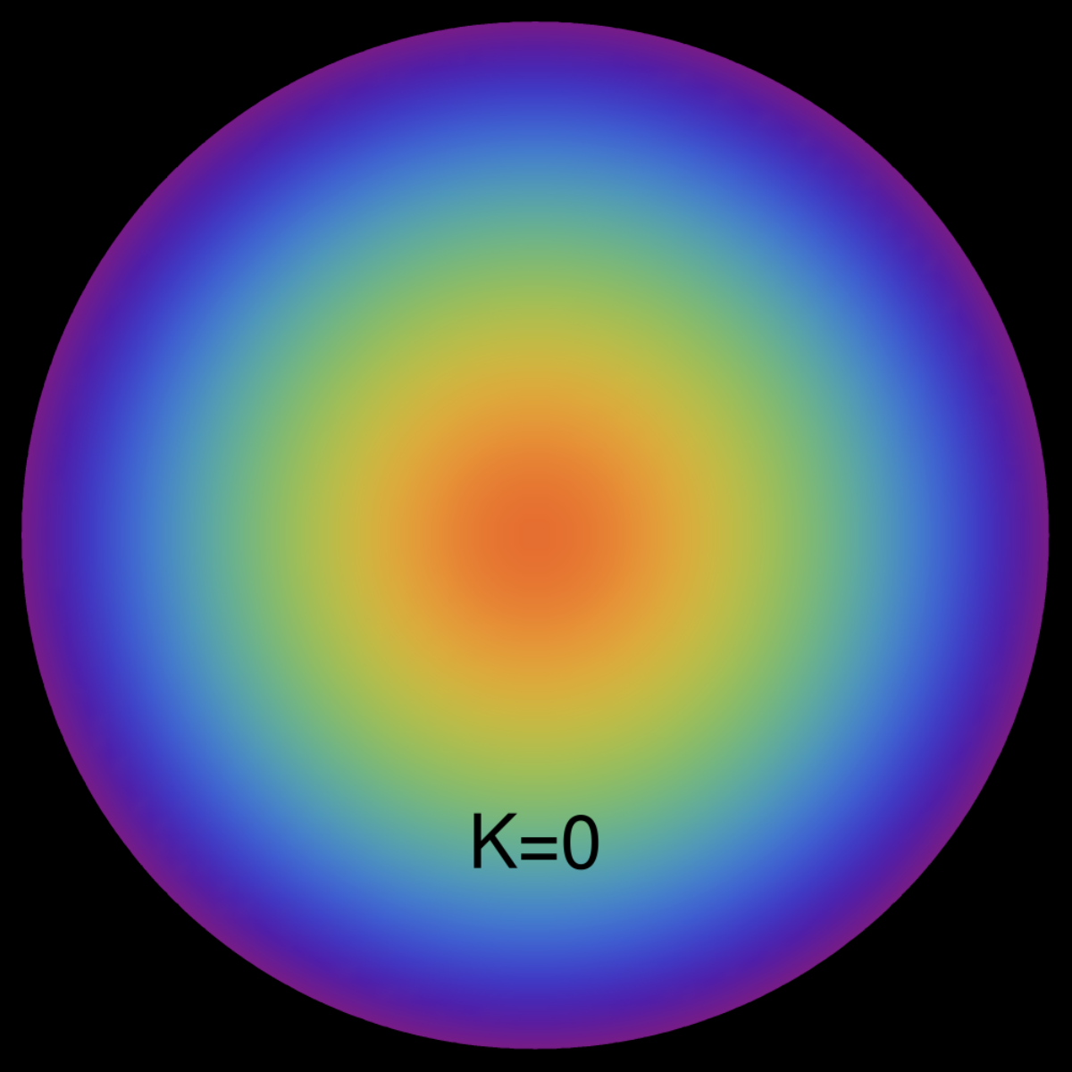
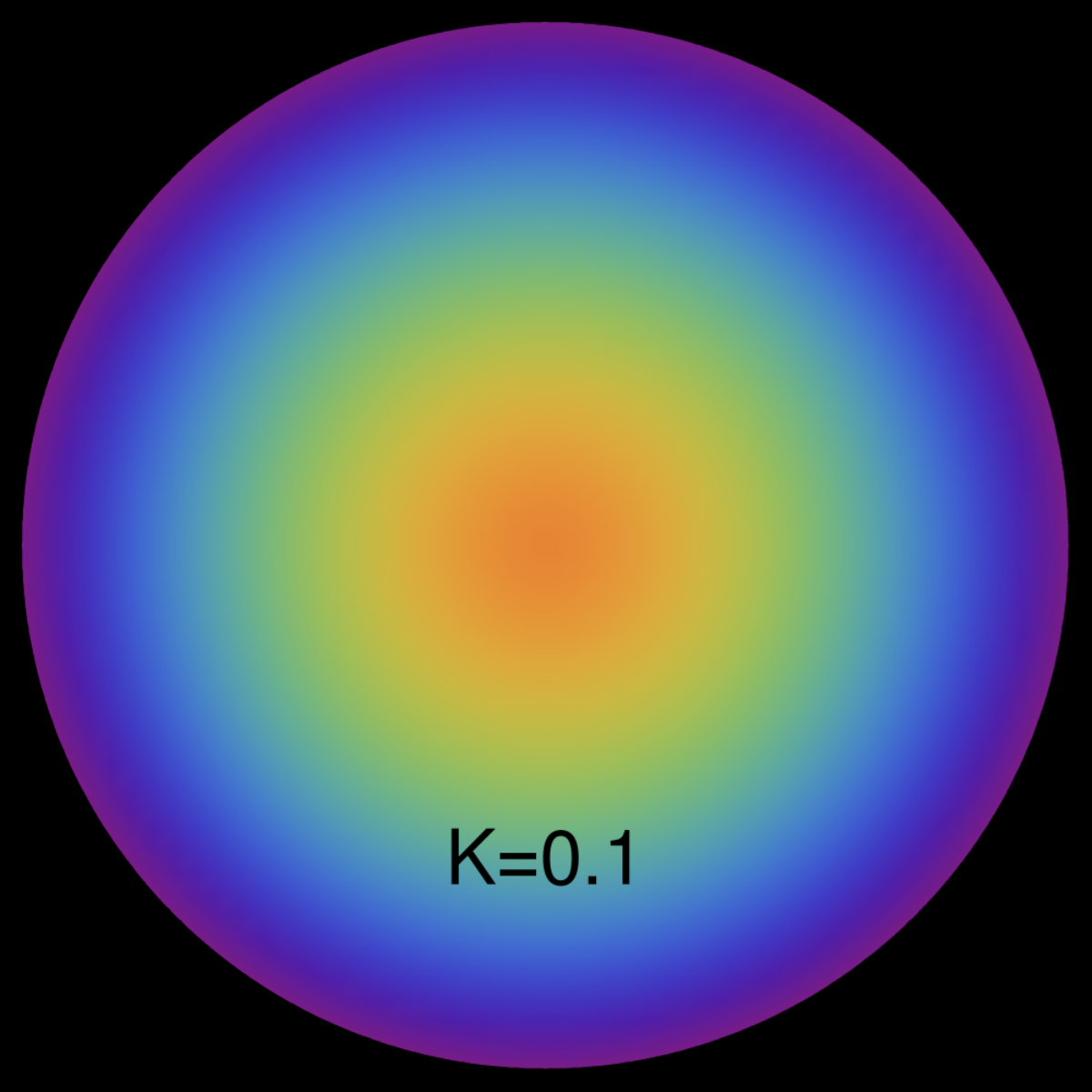
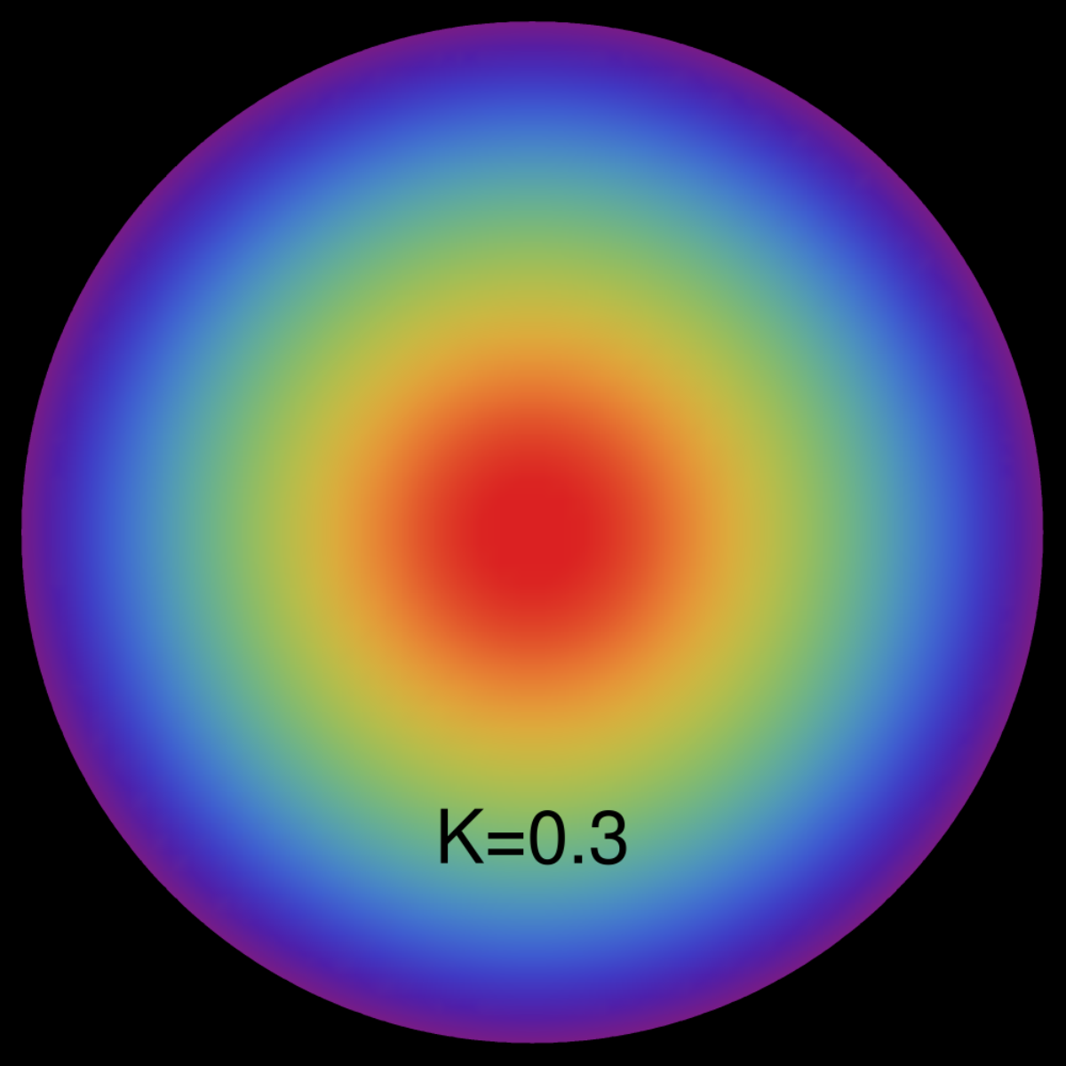
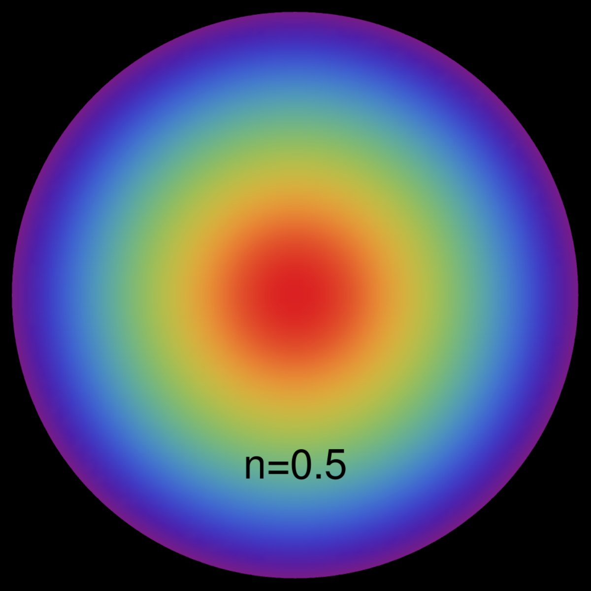
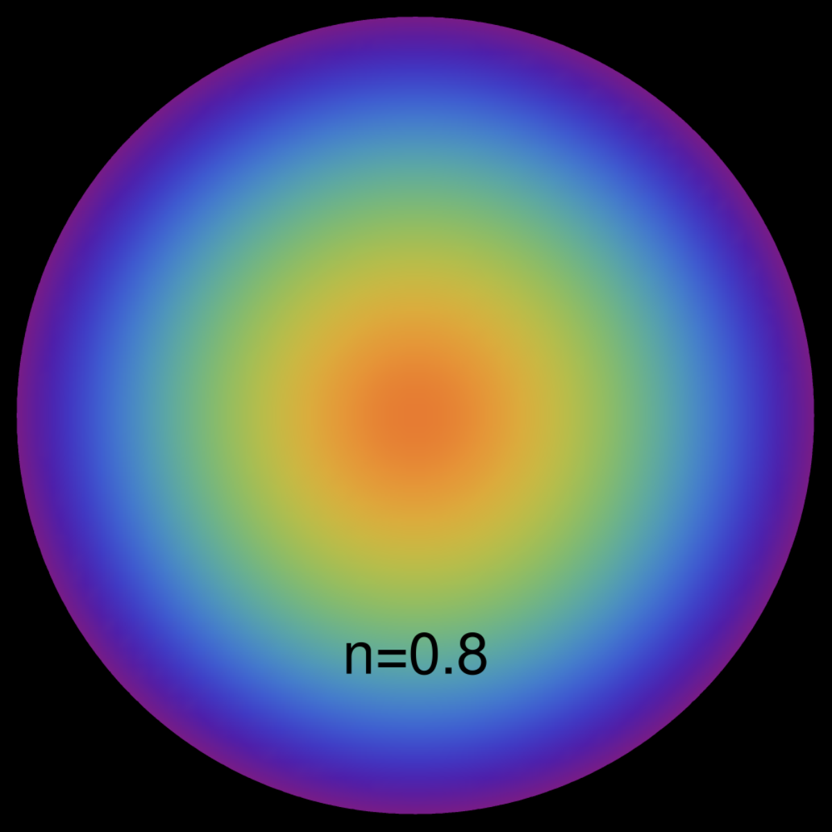
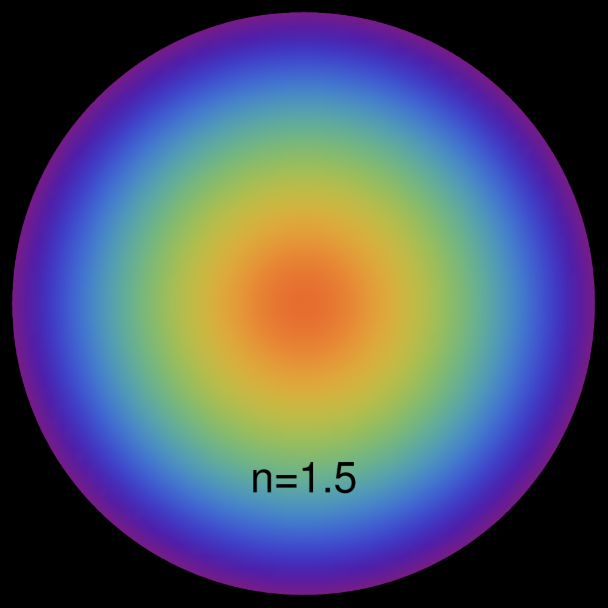
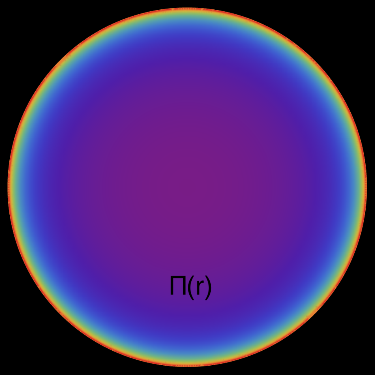
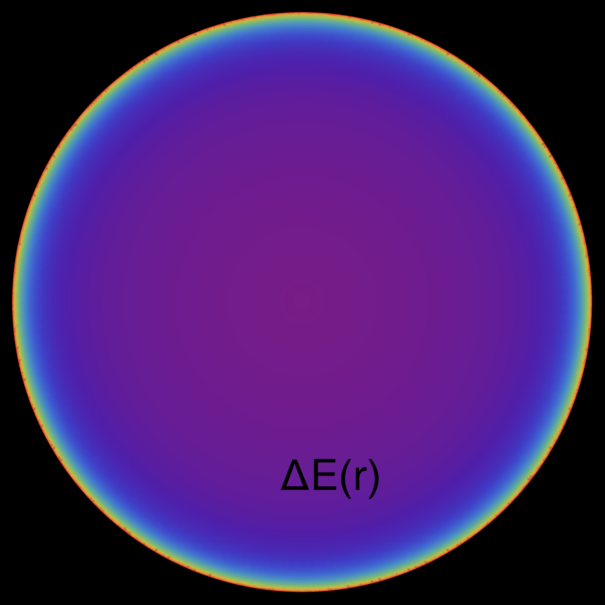
The tangential pressure, given by Eq. (11), also has an analytical expression in terms of (which converge rapidly), but it is too large to display. As we see, our solution does not require any perturbative analysis. Fig. 1 shows the pressure in Eq. (73) as a continuous function of the polytropic parameters . We see that the effects are greater for the innermost layers, and are always proportional to and . The same total effective pressure (73) is displayed in Figs. 2 and 3, now showing the effects of polytropes on stellar spheres explicitly. On the other hand, Fig. 4 shows the pressure and . Finally, the interaction between the polytope and the perfect fluid, which produces anisotropic consequences, is shown in Fig. 5. We see that the interaction between both fluids increases significantly near the stellar surface, and in fact, there is a positive gradient of energy in the radial direction. This could be interpreted as the necessary work done by the polytrope to keep the perfect fluid within the stellar volume. We conclude by mentioning that the strong energy condition is satisfied in all regions inside the stellar distribution.
V Conclusions
The study of relativistic fluids and their coexistence within self-gravitating systems is, in general, a complicated task to carry out. The reason for this lies in the complexity of Einstein’s field equations, which introduces nonlinear effects that are difficult to handle, even for simplest cases such as static and spherically symmetric systems. Despite this intrinsic and ineluctable difficulty, in this work we have developed a simple, analytical and direct strategy to study the effects of polytropes on any other relativistic fluid, regardless of the nature of the latter.
As a direct application, we study the case of a perfect fluid coexisting with a polytrope characterized by the parameters . To carry out the above, we use the well-known Tolman IV solution, which underlies in the limit , where all polytropic effects vanish. The total effective solution, formed by both fluids, is then analyzed, finding energy gradients that increase in the radial direction. These gradients are maximum on the stellar surface , as indicated in Fig. 5, and are positive (negative) for the polytrope (perfect fluid). This indicates that the polytrope needs to give up energy to achieve a coexistence with the perfect fluid compatible with the exterior Schwarzschild solution.
Finally, we want to point out that our solution satisfies the strong energy condition. However, it is necessary to carry out a more detailed study on its stability, and other questions that remain open, and that are beyond the goal of this work. For example, how much do our results depend on the chosen isotropic solution? How stable is the coexistence under radial perturbations? Likewise, the extension of this study to coexistence with other sources that are not necessarily isotropic remain open.
We want to conclude by emphasizing the direct impact of our approach on theories beyond Einstein, which can be described by a modified Einstein-Hilbert action as
where is the Ricci scalar, contains any matter fields appearing in the theory and the Lagrangian density of a new gravitational sector not described by general relativity, whose energy-momentum tensor is given by
Therefore, following our scheme, we can always study the possible exchange of energy between Einstein’s gravity and any other gravitational sector not described by general relativity.
Acknowledgments
J.O. is partially supported by ANID FONDECYT grant 1210041. EC is suported by Polygrant 17459
References
- Ovalle (2017) J. Ovalle, Phys. Rev. D95, 104019 (2017), arXiv:1704.05899 [gr-qc] .
- Ovalle (2019) J. Ovalle, Phys. Lett. B788, 213 (2019), arXiv:1812.03000 [gr-qc] .
- Contreras et al. (2021) E. Contreras, J. Ovalle, and R. Casadio, Phys. Rev. D 103, 044020 (2021), arXiv:2101.08569 [gr-qc] .
- Ovalle and Casadio (2020) J. Ovalle and R. Casadio, Beyond Einstein Gravity, SpringerBriefs in Physics (Springer Nature, Cham, 2020).
- da Rocha (2017a) R. da Rocha, Phys. Rev. D95, 124017 (2017a), arXiv:1701.00761 [hep-ph] .
- da Rocha (2017b) R. da Rocha, Eur. Phys. J. C77, 355 (2017b), arXiv:1703.01528 [hep-th] .
- Fernandes-Silva and da Rocha (2018) A. Fernandes-Silva and R. da Rocha, Eur. Phys. J. C78, 271 (2018), arXiv:1708.08686 [hep-th] .
- Casadio et al. (2018) R. Casadio, P. Nicolini, and R. da Rocha, Class. Quant. Grav. 35, 185001 (2018), arXiv:1709.09704 [hep-th] .
- Fernandes-Silva et al. (2018) A. Fernandes-Silva, A. J. Ferreira-Martins, and R. Da Rocha, Eur. Phys. J. C78, 631 (2018), arXiv:1803.03336 [hep-th] .
- Contreras and Bargueño (2018a) E. Contreras and P. Bargueño, Eur. Phys. J. C78, 558 (2018a), arXiv:1805.10565 [gr-qc] .
- Contreras (2018) E. Contreras, Eur. Phys. J. C78, 678 (2018), arXiv:1807.03252 [gr-qc] .
- Contreras and Bargueño (2018b) E. Contreras and P. Bargueño, Eur. Phys. J. C 78, 985 (2018b), arXiv:1809.09820 [gr-qc] .
- Panotopoulos and Rincón (2018) G. Panotopoulos and A. Rincón, Eur. Phys. J. C78, 851 (2018), arXiv:1810.08830 [gr-qc] .
- Da Rocha and Tomaz (2019) R. Da Rocha and A. A. Tomaz, Eur. Phys. J. C 79, 1035 (2019), arXiv:1905.01548 [hep-th] .
- Las Heras and León (2019) C. Las Heras and P. León, Eur. Phys. J. C 79, 990 (2019), arXiv:1905.02380 [gr-qc] .
- Rincón et al. (2019) A. Rincón, L. Gabbanelli, E. Contreras, and F. Tello-Ortiz, Eur. Phys. J. C 79, 873 (2019), arXiv:1909.00500 [gr-qc] .
- da Rocha (2020a) R. da Rocha, Symmetry 12, 508 (2020a), arXiv:2002.10972 [hep-th] .
- Contreras et al. (2020) E. Contreras, F. Tello-Ortiz, and S. K. Maurya, Class. Quant. Grav. 37, 155002 (2020), arXiv:2002.12444 [gr-qc] .
- Arias et al. (2020) C. Arias, F. Tello Ortiz, and E. Contreras, Eur. Phys. J. C 80, 463 (2020), arXiv:2003.00256 [gr-qc] .
- da Rocha (2020b) R. da Rocha, Phys. Rev. D 102, 024011 (2020b), arXiv:2003.12852 [hep-th] .
- Tello-Ortiz et al. (2020) F. Tello-Ortiz, S. Maurya, and Y. Gomez-Leyton, Eur. Phys. J. C 80, 324 (2020).
- da Rocha and Tomaz (2020) R. da Rocha and A. A. Tomaz, Eur. Phys. J. C 80, 857 (2020), arXiv:2005.02980 [hep-th] .
- Meert and da Rocha (2021) P. Meert and R. da Rocha, Nucl. Phys. B 967, 115420 (2021), arXiv:2006.02564 [gr-qc] .
- Tello-Ortiz et al. (2021) F. Tello-Ortiz, S. K. Maurya, and P. Bargueño, Eur. Phys. J. C 81, 426 (2021).
- Maurya and Nag (2021) S. K. Maurya and R. Nag, Eur. Phys. J. Plus 136, 679 (2021).
- Azmat and Zubair (2021a) H. Azmat and M. Zubair, Int. J. Mod. Phys. D 30, 2150115 (2021a).
- Maurya et al. (2022) S. K. Maurya, K. N. Singh, M. Govender, and S. Hansraj, Astrophys. J. 925, 208 (2022), arXiv:2109.00358 [gr-qc] .
- Ovalle et al. (2018a) J. Ovalle, R. Casadio, R. da Rocha, and A. Sotomayor, Eur. Phys. J. C78, 122 (2018a), arXiv:1708.00407 [gr-qc] .
- Gabbanelli et al. (2018) L. Gabbanelli, A. Rincón, and C. Rubio, Eur. Phys. J. C78, 370 (2018), arXiv:1802.08000 [gr-qc] .
- Heras and Leon (2018) C. L. Heras and P. Leon, Fortsch. Phys. 66, 1800036 (2018), arXiv:1804.06874 [gr-qc] .
- Estrada and Tello-Ortiz (2018) M. Estrada and F. Tello-Ortiz, Eur. Phys. J. Plus 133, 453 (2018), arXiv:1803.02344 [gr-qc] .
- Sharif and Sadiq (2018a) M. Sharif and S. Sadiq, Eur. Phys. J. C78, 410 (2018a), arXiv:1804.09616 [gr-qc] .
- Sharif and Sadiq (2018b) M. Sharif and S. Sadiq, Eur. Phys. J. Plus 133, 245 (2018b).
- Morales and Tello-Ortiz (2018) E. Morales and F. Tello-Ortiz, Eur. Phys. J. C78, 841 (2018), arXiv:1808.01699 [gr-qc] .
- Estrada and Prado (2019) M. Estrada and R. Prado, Eur. Phys. J. Plus 134, 168 (2019), arXiv:1809.03591 [gr-qc] .
- Sharif and Saba (2018) M. Sharif and S. Saba, Eur. Phys. J. C78, 921 (2018), arXiv:1811.08112 [gr-qc] .
- Ovalle et al. (2018b) J. Ovalle, R. Casadio, R. d. Rocha, A. Sotomayor, and Z. Stuchlik, Eur. Phys. J. C78, 960 (2018b), arXiv:1804.03468 [gr-qc] .
- Contreras (2019) E. Contreras, Class. Quant. Grav. 36, 095004 (2019), arXiv:1901.00231 [gr-qc] .
- Contreras et al. (2019) E. Contreras, A. Rincón, and P. Bargueño, Eur. Phys. J. C79, 216 (2019), arXiv:1902.02033 [gr-qc] .
- Contreras and Bargueño (2019) E. Contreras and P. Bargueño, Class. Quant. Grav. 36, 215009 (2019), arXiv:1902.09495 [gr-qc] .
- Gabbanelli et al. (2019) L. Gabbanelli, J. Ovalle, A. Sotomayor, Z. Stuchlik, and R. Casadio, Eur. Phys. J. C 79, 486 (2019), arXiv:1905.10162 [gr-qc] .
- Estrada (2019) M. Estrada, Eur. Phys. J. C 79, 918 (2019), arXiv:1905.12129 [gr-qc] .
- Ovalle et al. (2019) J. Ovalle, C. Posada, and Z. Stuchlík, Class. Quant. Grav. 36, 205010 (2019), arXiv:1905.12452 [gr-qc] .
- Hensh and Stuchlík (2019) S. Hensh and Z. Stuchlík, Eur. Phys. J. C 79, 834 (2019), arXiv:1906.08368 [gr-qc] .
- Linares Cedeño and Contreras (2020) F. X. Linares Cedeño and E. Contreras, Phys. Dark Univ. 28, 100543 (2020), arXiv:1907.04892 [gr-qc] .
- Torres-Sánchez and Contreras (2019) V. Torres-Sánchez and E. Contreras, Eur. Phys. J. C 79, 829 (2019), arXiv:1908.08194 [gr-qc] .
- Casadio et al. (2019) R. Casadio, E. Contreras, J. Ovalle, A. Sotomayor, and Z. Stuchlik, Eur. Phys. J. C 79, 826 (2019), arXiv:1909.01902 [gr-qc] .
- Singh et al. (2019) K. Singh, S. Maurya, M. Jasim, and F. Rahaman, Eur. Phys. J. C 79, 851 (2019).
- Maurya (2019) S. Maurya, Eur. Phys. J. C 79, 958 (2019).
- Sharif and Waseem (2019) M. Sharif and A. Waseem, Annals Phys. 405, 14 (2019).
- Abellan et al. (2020) G. Abellan, V. Torres-Sánchez, E. Fuenmayor, and E. Contreras, Eur. Phys. J. C 80, 177 (2020), arXiv:2001.08573 [gr-qc] .
- Sharif and Ama-Tul-Mughani (2020) M. Sharif and Q. Ama-Tul-Mughani, Annals Phys. 415, 168122 (2020), arXiv:2004.07925 [gr-qc] .
- Tello-Ortiz (2020) F. Tello-Ortiz, Eur. Phys. J. C 80, 413 (2020).
- Maurya (2020) S. Maurya, Eur. Phys. J. C 80, 429 (2020).
- Rincón et al. (2020) A. Rincón, E. Contreras, F. Tello-Ortiz, P. Bargueño, and G. Abellán, Eur. Phys. J. C 80, 490 (2020), arXiv:2005.10991 [gr-qc] .
- Sharif and Majid (2020) M. Sharif and A. Majid, Phys. Dark Univ. 30, 100610 (2020), arXiv:2006.04578 [gr-qc] .
- Maurya et al. (2020a) S. Maurya, K. N. Singh, and B. Dayanandan, Eur. Phys. J. C 80, 448 (2020a).
- Zubair and Azmat (2020) M. Zubair and H. Azmat, Annals Phys. 420, 168248 (2020), arXiv:2005.06955 [physics.gen-ph] .
- Sharif and Saba (2020) M. Sharif and S. Saba, Int. J. Mod. Phys. D 29, 2050041 (2020).
- Ovalle et al. (2021a) J. Ovalle, R. Casadio, E. Contreras, and A. Sotomayor, Phys. Dark Univ. 31, 100744 (2021a), arXiv:2006.06735 [gr-qc] .
- Estrada and Prado (2020) M. Estrada and R. Prado, Eur. Phys. J. C 80, 799 (2020), arXiv:2003.13168 [gr-qc] .
- Maurya et al. (2020b) S. K. Maurya, F. Tello-Ortiz, and M. K. Jasim, Eur. Phys. J. C 80, 918 (2020b).
- Maurya et al. (2021a) S. K. Maurya, F. Tello-Ortiz, and S. Ray, Phys. Dark Univ. 31, 100753 (2021a).
- Azmat and Zubair (2021b) H. Azmat and M. Zubair, Eur. Phys. J. Plus 136, 112 (2021b), arXiv:2106.08384 [gr-qc] .
- Islam and Ghosh (2021) S. U. Islam and S. G. Ghosh, Phys. Rev. D 103, 124052 (2021), arXiv:2102.08289 [gr-qc] .
- Afrin et al. (2021) M. Afrin, R. Kumar, and S. G. Ghosh, Mon. Not. Roy. Astron. Soc. 504, 5927 (2021), arXiv:2103.11417 [gr-qc] .
- Ovalle et al. (2021b) J. Ovalle, E. Contreras, and Z. Stuchlik, Phys. Rev. D 103, 084016 (2021b), arXiv:2104.06359 [gr-qc] .
- Ama-Tul-Mughani et al. (2021) Q. Ama-Tul-Mughani, W. us Salam, and R. Saleem, Eur. Phys. J. Plus 136, 426 (2021).
- Sharif and Aslam (2021) M. Sharif and M. Aslam, Eur. Phys. J. C 81, 641 (2021), arXiv:2107.12968 [gr-qc] .
- da Rocha (2021) R. da Rocha, Eur. Phys. J. C 81, 845 (2021), arXiv:2107.13483 [gr-qc] .
- Maurya et al. (2021b) S. K. Maurya, A. M. Al Aamri, A. K. Al Aamri, and R. Nag, Eur. Phys. J. C 81, 701 (2021b).
- Carrasco-Hidalgo and Contreras (2021) M. Carrasco-Hidalgo and E. Contreras, Eur. Phys. J. C 81, 757 (2021), arXiv:2108.10311 [gr-qc] .
- Sultana (2021) J. Sultana, Symmetry 13, 1598 (2021).
- da Rocha (2022) R. da Rocha, Eur. Phys. J. C 82, 34 (2022), arXiv:2111.11995 [gr-qc] .
- Maurya and Nag (2022) S. K. Maurya and R. Nag, Eur. Phys. J. C 82, 48 (2022), arXiv:2112.01497 [gr-qc] .
- Omwoyo et al. (2021) E. Omwoyo, H. Belich, J. C. Fabris, and H. Velten, (2021), arXiv:2112.14124 [gr-qc] .
- Afrin and Ghosh (2022) M. Afrin and S. G. Ghosh, Universe 8, 52 (2022), arXiv:2112.15038 [gr-qc] .
- Meert and da Rocha (2022) P. Meert and R. da Rocha, Eur. Phys. J. C 82, 175 (2022), arXiv:2109.06289 [hep-th] .
- Horedt (2004) G. P. Horedt, Polytropes , Astrophysics and Space Science Library (Springer, Dordrecht, 2004).
- Herrera and Barreto (2013) L. Herrera and W. Barreto, Phys. Rev. D 88, 084022 (2013), arXiv:1310.1114 [gr-qc] .
- Stuchlík et al. (2016) Z. Stuchlík, S. Hledík, and J. Novotný, Phys. Rev. D94, 103513 (2016), arXiv:1611.05327 [gr-qc] .
- Stuchlik (2000) Z. Stuchlik, Acta Phys. Slov. 50, 219 (2000), arXiv:0803.2530 [gr-qc] .
- Novotný et al. (2017) J. Novotný, J. Hladík, and Z. Stuchlík, Phys. Rev. D 95, 043009 (2017), arXiv:1703.04604 [gr-qc] .
- Stuchlík et al. (2017) Z. Stuchlík, J. Schee, B. Toshmatov, J. Hladík, and J. Novotny, JCAP 1706, 056 (2017), arXiv:1704.07713 [gr-qc] .
- Posada et al. (2020) C. Posada, J. Hladík, and Z. Stuchlík, Phys. Rev. D 102, 024056 (2020), arXiv:2005.14072 [gr-qc] .
- Tolman (1939) R. C. Tolman, Phys. Rev. 55, 364 (1939).