跳到论文正文
W Papers独立论文阅读器 arXiv:2202.12658 论文正文 计算阅读时间 · 0%
引用这篇论文根据当前论文元数据生成,正式投稿前建议核对。


License: arXiv.org perpetual non-exclusive license
arXiv:2202.12658v1 [math.NA] 25 Feb 2022

Convergence of sparse grid Gaussian convolution approximation for multi-dimensional periodic functions

Simon Hubbert Note: Department of Economics, Mathematics and Statistics, Birkbeck, University of London, WC1H 7HX, UK. s.hubbert@bbk.ac.uk    Janin Jäger Note: Lehrstuhl Numerische Mathematik, Justus-Liebig University, 35392 Giessen, Germany. janin.jaeger@math.uni-giessen.de    Jeremy Levesley Note: Department of Mathematics, University of Leicester, LE1 7RH, UK. jl1@le.ac.uk
Abstract

We consider the problem of approximating [0,1]d[0,1]^{d}-periodic functions by convolution with a scaled Gaussian kernel. We start by establishing convergence rates to functions from periodic Sobolev spaces and we show that the saturation rate is O⁡(h2),O(h^{2}), where hh is the scale of the Gaussian kernel. Taken from a discrete point of view, this result can be interpreted as the accuracy that can be achieved on the uniform grid with spacing h.h. In the discrete setting, the curse of dimensionality would place severe restrictions on the computation of the approximation. For instance, a spacing of 2−n2^{-n} would provide an approximation converging at a rate of O⁡(2−2​n)O(2^{-2n}) but would require (2n+1)d(2^{n}+1)^{d} grid points. To overcome this we introduce a sparse grid version of Gaussian convolution approximation, where substantially fewer grid points are required, and show that the sparse grid version delivers a saturation rate of O⁡(nd−1​2−2​n).O(n^{d-1}2^{-2n}). This rate is in line with what one would expect in the sparse grid setting (where the full grid error only deteriorates by a factor of order nd−1n^{d-1}) however the analysis that leads to the result is novel in that it draws on results from the theory of special functions and key observations regarding the form of certain weighted geometric sums.

1 Introduction

Many methods that are designed to deliver approximations are based on the convolution of a kernel function with the function being approximated. The general approach involves selecting a suitable integrable function K:I​Rd→I​RK:{\rm I}\!{\rm R}^{d}\to{\rm I}\!{\rm R} (the convolution kernel) satisfying

∫I​RdK(𝐱)d𝐱=∫I​RdK(x1,…,xd)dx1⋯dxd=1.\int_{{\rm I}\!{\rm R}^{d}}K({\bf{x}})d{\bf{x}}=\int_{{\rm I}\!{\rm R}^{d}}K(x_{1},\ldots,x_{d})dx_{1}\cdots dx_{d}=1.

A scaling vector 𝐡=(h1,…,hd)T∈I​Rd,{\bf{h}}=(h_{1},\ldots,h_{d})^{T}\in{\rm I}\!{\rm R}^{d}, with hi>0h_{i}>0 (1≤i≤d1\leq i\leq d) is then used to define a parameterised family of convolution kernels by

K𝐡​(𝐱)=1h1⋯hd​K​(x1h1,…,xdhd).K_{{\bf{h}}}({\bf{x}})=\frac{1}{h_{1}\cdots h_{d}}K\left(\frac{x_{1}}{h_{1}},\ldots,\frac{x_{d}}{h_{d}}\right).

The convolution approximation to a function f∈L1​(I​Rd)f\in L_{1}({\rm I}\!{\rm R}^{d}) is defined by

𝒞h​(f)​(x)=(f∗K𝐡)​(𝐱)=∫I​Rdf⁡(𝐲)​K𝐡​(𝐱−𝐲)​𝑑𝐲.{{\mathcal{C}_{\textbf{h}}(f)(\textbf{x})=(f\ast K_{{\bf{h}}})({\bf{x}})=\int_{{\rm I}\!{\rm R}^{d}}f({\bf{y}})K_{{\bf{h}}}({\bf{x}}-{\bf{y}})d{\bf{y}}.}} (1.1)

The convolution kernel described above is anisotropic as each direction is allowed to be scaled by its own factor. This is practically useful because a typical data sample of a function will show variety along different directions and so a well designed anisotropic scaling can efficiently capture these features. However, from a theoretical perspective, most convergence results relate to the isotropic scale where each direction is scaled by the same factor h>0.h>0. In this case the scaled kernel is Kh​(𝐱)=h−d​K​(𝐱h)K_{h}({\bf{x}})=h^{-d}K\left(\frac{{\bf{x}}}{h}\right) and the corresponding convolution approximation

𝒞h​(f)​(𝐱)=∫I​Rdf⁡(𝐲)​Kh​(𝐱−𝐲)​d𝐲=1hd​∫I​Rdf⁡(𝐲)​K​(𝐱−𝐲h)​d𝐲,\displaystyle{\cal{C}}_{h}(f)({\bf{x}})=\int_{{\rm I}\!{\rm R}^{d}}f({\bf{y}})K_{h}({\bf{x}}-{\bf{y}})d{\bf{y}}=\frac{1}{h^{d}}\int_{{\rm I}\!{\rm R}^{d}}f({\bf{y}})K\left(\frac{{\bf{x}}-{\bf{y}}}{h}\right)d{\bf{y}}, (1.2)

can be shown to converge to ff as h→0h\to 0, the convergence being uniform on compact sets, [4] chapter 20, theorem 2. The rate of convergence depends upon the smoothness of ff and the polynomial reproduction properties of the underlying kernel. The convolution approximation can be viewed as the continuous counterpart of quasi-interpolation; a discrete method which generates an approximation over the whole of I​Rd{\rm I}\!{\rm R}^{d} by linearly combining the values of ff sampled at the scaled integer lattice h​𝐙dh{{{\mathbf{Z}}}}^{d} together with the appropriately shifted and scaled kernel function. The classical construction, as for example described in [3], takes the form

Qh​(f)​(𝐱)=∑𝐤∈𝐙df⁡(𝐤​h)​K​(𝐱h−𝐤),𝐱∈I​Rd,h>0.{{Q_{h}(f)({\bf{x}})=\sum_{{\bf{k}}\in{{{\mathbf{Z}}}}^{d}}f({\bf{k}}h)K\left(\frac{{\bf{x}}}{h}-{\bf{k}}\right),\quad{\bf{x}}\in{\rm I}\!{\rm R}^{d},\quad h>0.}} (1.3)

Following [9] the connection between continuous convolution and discrete quasi-interpolation can be seen if we write

𝒞h​(f)​(𝐱)=1hd​∑𝐤∈𝐙d∫h⋅(𝐤+[−12,12]d)f⁡(𝐲)​K​(𝐱−𝐲h)​d𝐲.\displaystyle{\cal{C}}_{h}(f)({\bf{x}})=\frac{1}{h^{d}}\sum_{{\bf{k}}\in{{\mathbf{Z}}}^{d}}\int_{h\cdot({\bf{k}}+[-\frac{1}{2},\frac{1}{2}]^{d})}f({\bf{y}})K\left(\frac{{\bf{x}}-{\bf{y}}}{h}\right)d{\bf{y}}.

The integrals above are taken over appropriately shifted and scaled versions of the cube [−12,12]d.[-\frac{1}{2},\frac{1}{2}]^{d}. If we approximate each integrand by its value at the midpoint of the cube we get

∫h⋅(𝐤+[−12,12]d)f⁡(𝐲)​K​(𝐱−𝐲h)​𝑑𝐲≈hd​f​(𝐤​h)​K​(𝐱h−𝐤),\int_{h\cdot({\bf{k}}+[-\frac{1}{2},\frac{1}{2}]^{d})}f({\bf{y}})K\left(\frac{{\bf{x}}-{\bf{y}}}{h}\right)d{\bf{y}}\approx h^{d}f({\bf{k}}h)K\left(\frac{{\bf{x}}}{h}-{\bf{k}}\right),

and so we have that 𝒞h​(f)​(𝐱)≈Qh​(f)​(𝐱).{\cal{C}}_{h}(f)({\bf{x}})\approx Q_{h}(f)({\bf{x}}). Quasi-interpolation using Gaussians in one dimension was described in [8].

In this paper we will examine the approximation of [0,1]d−[0,1]^{d}-periodic functions by convolution with the multi-dimensional Gaussian kernel. Given the close connection of continuous convolution to quasi-interpolation the results we establish in the continuous setting will serve as a baseline for what should be expected in the discrete case.

We begin in Section 2 by deriving the formula for the Fourier expansion of the pointwise error using the anisotropic scaling of the Gaussian; this result allows us to deduce that convolution approximation is only able to reproduce the constant function. We then analyse the isotropic case in some detail. In this setting we demonstrate that the convergence has a saturation rate of 𝒪⁡(h2){\cal{O}}(h^{2}).

In Section 3 we consider the practical issues of employing the discrete (quasi-interpolation) analogue of continuous convolution in high dimensions. Such a recasting involves constructing a full grid in [0,1]d[0,1]^{d} with an isotropic spacing of h=12n,h=\frac{1}{2^{n}}, where nn is a positive integer. In this setting, the convolution approximation will converge to ff at a rate of 122​n,\frac{1}{2^{2n}}, provided ff is sufficiently smooth. However, in the discrete setting we are restricted by the curse of dimensionality since the construction of the quasi-interpolant would require (2n+1)d(2^{n}+1)^{d} evaluations and this is prohibitively large as nn grows. In order to overcome this we consider replacing the full-grid approximation with a sparse grid version which is built from a certain linear combination of smaller full grid approximations. Numerical experiments on closely connected methods have been published in [12]. To analyse this theoretically we mimic the approach of Section 2, i.e., we first derive the formula for the Fourier expansion of the pointwise error using the sparse grid convolution approximation. We then investigate the Fourier coefficients of the error expansion and we state the main theorem of the paper, concerning the decay rate of the coefficients. We then establish that, provided ff is sufficiently smooth, the sparse grid convolution approximation will converge to ff at a rate of nd−122​n.\frac{n^{d-1}}{2^{2n}}. Section 4 is devoted to the proof of the aforementioned main theorem of the paper.

2 Gaussian convolution approximation

Our choice of convolution kernel is the multi-dimensional Gaussian

Ψ⁡(𝐱)=1(2​π)d2​exp⁡(−12​𝐱T​𝐱)=1(2​π)d2​exp⁡(−12​(∑i=1dxi2))=∏i=1dψ⁡(xi),\displaystyle\Psi({\bf{x}})=\frac{1}{(2\pi)^{\frac{d}{2}}}\exp\left(-\frac{1}{2}{\bf{x}}^{T}{\bf{x}}\right)=\frac{1}{(2\pi)^{\frac{d}{2}}}\exp\left(-\frac{1}{2}\left(\sum_{i=1}^{d}x_{i}^{2}\right)\right)=\prod_{i=1}^{d}\psi(x_{i}),

where ψ:I​R→I​R\psi:{\rm I}\!{\rm R}\to{\rm I}\!{\rm R} is the univariate Gaussian ψ⁡(x)=(2​π)−12​exp⁡(−12​x2).\psi(x)=(2\pi)^{-\frac{1}{2}}\exp\left(-\frac{1}{2}x^{2}\right). Fourier theory will play an important role in our analysis and we recall that if we let ex​(z)=exp⁡(2​π​i​x⋅z)e_{x}(z)=\exp(2\pi ix\cdot z) then the univariate Fourier transform of ψ\psi is

ψ^​(z):=∫−∞∞ψ⁡(x)​e−x​(z)​𝑑x=exp⁡(−2​π2​z2).\widehat{\psi}(z):=\int_{-\infty}^{\infty}\psi(x)e_{-x}(z)dx=\exp(-2\pi^{2}z^{2}).

Our general aim is to approximate a [0,1]d[0,1]^{d}-periodic function

f⁡(𝐱)=∑𝐤∈𝐙df^​(𝐤)​e𝐤​(𝐱)wheree𝐲​(𝐱):=exp⁡(2​π​i​𝐲T​𝐱)=∏i=1deyi​(xi),f({\bf{x}})=\sum_{{\bf{k}}\in{{\mathbf{Z}}}^{d}}{\widehat{f}({\bf{k}})}e_{{\bf{k}}}({\bf{x}})\quad{\rm{where}}\quad e_{{\bf{y}}}({\bf{x}}):=\exp(2\pi i{\bf{y}}^{T}{\bf{x}})=\prod_{i=1}^{d}e_{y_{i}}(x_{i}),

by the continuous multi-variable convolution

𝒞𝐡​(f)=∫I​Rdf⁡(z)​Ψh​(x−z)​dz=∑j∈𝐙d∫[0,1]df⁡(z)​Ψh​(x−z−j)​dz=∫[0,1]df⁡(z)​Φh​(x−z)​dz,\displaystyle\mathcal{C}_{{\bf{h}}}(f)=\int_{{\rm I}\!{\rm R}^{d}}f(\textbf{z})\Psi_{\textbf{h}}(\textbf{x}-\textbf{z})d\textbf{z}=\sum_{\textbf{j}\in{{\mathbf{Z}}}^{d}}\int_{[0,1]^{d}}f(\textbf{z})\Psi_{\textbf{h}}(\textbf{x}-\textbf{z}-\textbf{j})d\textbf{z}=\int_{[0,1]^{d}}f(\textbf{z})\Phi_{\textbf{h}}(\textbf{x}-\textbf{z})d\textbf{z},

where

Φh​(x)=∑j∈𝐙dΨh​(x−j).\Phi_{\textbf{h}}(\textbf{x})=\sum_{\textbf{j}\in{{\mathbf{Z}}}^{d}}\Psi_{\textbf{h}}(\textbf{x}-\textbf{j}).

Now, Φh​(x)\Phi_{\textbf{h}}(\textbf{x}) is [0,1]d−[0,1]^{d}-periodic and so has a multi-dimensional Fourier series

Φh​(x)=∑k∈𝐙dΦh^​(k)​ek​(x),\Phi_{\textbf{h}}(\textbf{x})=\sum_{\textbf{k}\in{{\mathbf{Z}}}^{d}}\widehat{\Phi_{\textbf{h}}}(\textbf{k})e_{\textbf{k}}(\textbf{x}),

where

Φh^​(k)\displaystyle\widehat{\Phi_{\textbf{h}}}(\textbf{k}) =∫[0,1]dΦh​(x)​e−k​(x)​𝐝x\displaystyle=\int_{[0,1]^{d}}\Phi_{\textbf{h}}(\textbf{x})e_{-\textbf{k}}(\textbf{x})d\textbf{x}
=∫[0,1]d(∑j∈𝐙dΨh​(x−j))​e−k​(x)​𝐝x\displaystyle=\int_{[0,1]^{d}}\left(\sum_{\textbf{j}\in{{\mathbf{Z}}}^{d}}\Psi_{\textbf{h}}(\textbf{x}-\textbf{j})\right)e_{-\textbf{k}}(\textbf{x})d\textbf{x}
=∑j∈𝐙d∫[0,1]dΨh​(x−j)​e−k​(x)​𝐝x\displaystyle=\sum_{\textbf{j}\in{{\mathbf{Z}}}^{d}}\int_{[0,1]^{d}}\Psi_{\textbf{h}}(\textbf{x}-\textbf{j})e_{-\textbf{k}}(\textbf{x})d\textbf{x}
=∫I​RdΨh​(x)​e−k​(x)​dx=∏i=1d∫−∞∞ψhi​(xi)​e−ki​(xi)​d​xi=∏i=1dψ^​(hi​ki).\displaystyle=\int_{{\rm I}\!{\rm R}^{d}}\Psi_{\textbf{h}}(\textbf{x})e_{-\textbf{k}}(\textbf{x})d\textbf{x}=\prod_{i=1}^{d}\int_{-\infty}^{\infty}\psi_{h_{i}}(x_{i})e_{-k_{i}}(x_{i})dx_{i}=\prod_{i=1}^{d}\widehat{\psi}(h_{i}k_{i}).

Applying the dd-dimensional convolution formula for [0,1]d−[0,1]^{d}-periodic functions we have:

𝒞𝐡​(f)​(x)=∑k∈𝐙df^​(k)​Φh^​(k)​ek​(x)=∑k∈𝐙df^​(k)​(∏i=1dψ^​(hi​ki))​ek​(x).\displaystyle\mathcal{C}_{{\bf{h}}}(f)(\textbf{x})=\sum_{\textbf{k}\in{{\mathbf{Z}}}^{d}}\widehat{f}(\textbf{k})\widehat{\Phi_{\textbf{h}}}(\textbf{k})e_{\textbf{k}}(\textbf{x})=\sum_{\textbf{k}\in{{\mathbf{Z}}}^{d}}\widehat{f}(\textbf{k})\left(\prod_{i=1}^{d}\widehat{\psi}(h_{i}k_{i})\right)e_{\textbf{k}}(\textbf{x}). (2.1)

Thus the error in the convolution approximation is

Eh​(f)​(𝐱)=f⁡(𝐱)−𝒞𝐡​(f)​(x)=∑𝐤∈𝐙df^​(k)​(1−(∏i=1dψ^​(hi​ki)))​ek​(x).\displaystyle E_{\textbf{h}}(f)({\bf{x}})=f({\bf{x}})-\mathcal{C}_{{\bf{h}}}(f)(\textbf{x})=\sum_{{\bf{k}}\in{{\mathbf{Z}}}^{d}}\widehat{f}(\textbf{k})\left(1-\left(\prod_{i=1}^{d}\widehat{\psi}(h_{i}k_{i})\right)\right)e_{\textbf{k}}(\textbf{x}). (2.2)

We note that, since ψ^​(0)=1,\widehat{\psi}(0)=1, the above error representation immediately shows that the convolution reproduces the constant but not any other trigonometric polynomial.

2.1 Convergence with Isotropic scaling

If we consider the isotropic case where the same scale factor hh is applied to all coordinate directions then (2.2) can be written as

Eh​(f)​(𝐱)=∑𝐤∈𝐙d∖{𝟎}f^​(k)​(1−e−2​π2​h2​‖𝐤‖2)​ek​(x).{{E_{h}(f)({\bf{x}})=\sum_{{\bf{k}}\in{{\mathbf{Z}}}^{d}\setminus\{{\bf{0}}\}}\widehat{f}(\textbf{k})\left(1-e^{-2\pi^{2}h^{2}\|{\bf{k}}\|^{2}}\right)e_{\textbf{k}}(\textbf{x}).}} (2.3)

The functions we wish to approximate are taken from a periodic Sobolev space

𝒩β={f=∑𝐤∈𝐙df^​(𝐤)​e𝐤:‖f‖β=(∑k∈𝐙d∖{0}‖k‖2​β​|f^​(𝐤)|2)1/2<∞}.\mathcal{N}_{\beta}=\left\{f=\sum_{{\bf{k}}\in{{\mathbf{Z}}}^{d}}{\widehat{f}({\bf{k}})}e_{\bf{k}}:\|f\|_{\beta}=\left(\sum_{\textbf{k}\in{{\mathbf{Z}}}^{d}\setminus\{{\textbf{0}}\}}\|\textbf{k}\|^{2\beta}|{\widehat{f}({\bf{k}})}|^{2}\right)^{1/2}<\infty\right\}.

The Sobolev embedding theorem [2] ensures that if β>d2\beta>\frac{d}{2} then all functions in 𝒩β\mathcal{N}_{\beta} will be continuous. The following result gives error bounds for Gaussian convolution approximation of such functions.

Proposition 2.1. Let f∈𝒩β,f\in\mathcal{N}_{\beta}, where β>d2.\beta>\frac{d}{2}. Then

‖Eh​f‖∞≤‖f‖β⋅{C1​h2for​β>d2+2;h2​(C2​ln⁡(1h)+C3)for​β=d2+2;C4​hβ−d2for​d2<β<d2+2,\|E_{h}f\|_{\infty}\leq\|f\|_{\beta}\cdot\begin{cases}C_{1}h^{2}\,\,&\,\,\textrm{for}\,\,\,\,\beta>\frac{d}{2}+2;\\ h^{2}\left(C_{2}\sqrt{\ln\left(\frac{1}{h}\right)}+C_{3}\right)\,\,&\,\,\textrm{for}\,\,\,\,\beta=\frac{d}{2}+2;\\ C_{4}h^{\beta-\frac{d}{2}}\,\,&\,\,\textrm{for}\,\,\,\,\frac{d}{2}<\beta<\frac{d}{2}+2,\end{cases}

where CiC_{i} i=1,2,3,4i=1,2,3,4, are positive constants independent of h.h.

Proof.

Using (2.3) together with the elementary bound 1−e−x<x1-e^{-x}<x (for OPENx>0),x>0), we can deduce that

‖Eh​f‖∞≤2​π2​h2​∑𝐤∈𝐙d∖{𝟎}‖𝐤‖2​|f^​(𝐤)|.{{\|E_{h}f\|_{\infty}\leq 2\pi^{2}h^{2}\sum_{{\bf{k}}\in{{\mathbf{Z}}}^{d}\setminus\{{\bf{0}}\}}\|{\bf{k}}\|^{2}|{\widehat{f}({\bf{k}})}|.}} (2.4)

Suppose that β=d2+2+α,\beta=\frac{d}{2}+2+\alpha, where α>0,\alpha>0, then an application of the Cauchy Schwarz inequality yields

‖Eh​f‖∞\displaystyle\|E_{h}f\|_{\infty} ≤2​π2​h2​∑𝐤∈𝐙d∖{𝟎}1‖𝐤‖d2+α⋅‖𝐤‖d2+α+2​|f^​(𝐤)|\displaystyle\leq 2\pi^{2}h^{2}\sum_{{\bf{k}}\in{{\mathbf{Z}}}^{d}\setminus\{{\bf{0}}\}}\frac{1}{\|{\bf{k}}\|^{\frac{d}{2}+\alpha}}\cdot\|{\bf{k}}\|^{\frac{d}{2}+\alpha+2}|{\widehat{f}({\bf{k}})}|
≤2​π2​h2​(∑𝐤∈𝐙d∖{𝟎}1‖𝐤‖d+2​α)12⋅(∑𝐤∈𝐙d∖{𝟎}(‖𝐤‖2)d2+2+α​|f^​(𝐤)|2)12\displaystyle\leq 2\pi^{2}h^{2}\left(\sum_{{\bf{k}}\in{{\mathbf{Z}}}^{d}\setminus\{{\bf{0}}\}}\frac{1}{\|{\bf{k}}\|^{d+2\alpha}}\right)^{\frac{1}{2}}\cdot\left(\sum_{{\bf{k}}\in{{\mathbf{Z}}}^{d}\setminus\{{\bf{0}}\}}\left(\|{\bf{k}}\|^{2}\right)^{\frac{d}{2}+2+\alpha}|{\widehat{f}({\bf{k}})}|^{2}\right)^{\frac{1}{2}}
≤2​π2​C​h2​‖f‖β.\displaystyle\leq 2\pi^{2}Ch^{2}\|f\|_{\beta}.

Now assume that β=d2+2−α\beta=\frac{d}{2}+2-\alpha where 0<α<2.0<\alpha<2. In the following development we will work with a partition of the punctured integer lattice

𝐙d∖{𝟎}={𝐤∈𝐙d∖{𝟎}:1≤‖𝐤‖<1h}⏟=Θh∪{𝐤∈𝐙d:‖𝐤‖≥1h}⏟=Γh.{{\mathbf{Z}}}^{d}\setminus\{{\bf{0}}\}=\underbrace{\left\{{\bf{k}}\in{{\mathbf{Z}}}^{d}\setminus\{{\bf{0}}\}:1\leq\|{\bf{k}}\|<\frac{1}{h}\right\}}_{=\Theta_{h}}\cup\underbrace{\left\{{\bf{k}}\in{{\mathbf{Z}}}^{d}:\|{\bf{k}}\|\geq\frac{1}{h}\right\}}_{=\Gamma_{h}}.

Using this we bound the error in two parts as follows

‖Eh​f‖∞≤∑𝐤∈Θh|f^​(𝐤)|⋅|1−e−2​π2​h2​‖𝐤‖2|+∑𝐤∈Γh|f^​(𝐤)|⋅|1−e−2​π2​h2​‖𝐤‖2|.\|E_{h}f\|_{\infty}\leq\sum_{\mathbf{k}\in\Theta_{h}}|{\widehat{f}({\bf{k}})}|\cdot|1-e^{-2\pi^{2}h^{2}\|\mathbf{k}\|^{2}}|+\sum_{\mathbf{k}\in\Gamma_{h}}|{\widehat{f}({\bf{k}})}|\cdot|1-e^{-2\pi^{2}h^{2}\|\mathbf{k}\|^{2}}|.

For the sum over Θh\Theta_{h} we again employ 1−e−x<x1-e^{-x}<x and, bounding as before, we conclude that

∑𝐤∈Θh|f^​(𝐤)|⋅|1−e−2​π2​h2​‖𝐤‖2|≤2​π2​h2​∑𝐤∈Θh|f^​(𝐤)|⋅‖𝐤‖2\displaystyle\sum_{\mathbf{k}\in\Theta_{h}}|{\widehat{f}({\bf{k}})}|\cdot|1-e^{-2\pi^{2}h^{2}\|\mathbf{k}\|^{2}}|\leq 2\pi^{2}h^{2}\sum_{\mathbf{k}\in\Theta_{h}}|{\widehat{f}({\bf{k}})}|\cdot\|\mathbf{k}\|^{2}
=2​π2​h2​∑𝐤∈Θh‖𝐤‖α−d2​‖𝐤‖d2+2−α​|f^​(𝐤)|\displaystyle=2\pi^{2}h^{2}\sum_{\mathbf{k}\in\Theta_{h}}\|\mathbf{k}\|^{\alpha-\frac{d}{2}}\|\mathbf{k}\|^{\frac{d}{2}+2-\alpha}|{\widehat{f}({\bf{k}})}|
≤2​π2​h2​(∑𝐤∈Θh‖𝐤‖2​α−d)12​(∑𝐤∈Θh(‖𝐤‖2)d2+2−α​|f^​(𝐤)|2)12\displaystyle\leq 2\pi^{2}h^{2}\left(\sum_{\mathbf{k}\in\Theta_{h}}\|\mathbf{k}\|^{2\alpha-d}\right)^{\frac{1}{2}}\left(\sum_{\mathbf{k}\in\Theta_{h}}\left(\|\mathbf{k}\|^{2}\right)^{\frac{d}{2}+2-\alpha}|{\widehat{f}({\bf{k}})}|^{2}\right)^{\frac{1}{2}}
≤2​π2​h2​(∑𝐤∈Θh(1h)2​α−d)12​‖f‖d2+2−α\displaystyle\leq 2\pi^{2}h^{2}\left(\sum_{\mathbf{k}\in\Theta_{h}}\left(\frac{1}{h}\right)^{2\alpha-d}\right)^{\frac{1}{2}}\|f\|_{\frac{d}{2}+2-\alpha}
≤C⋅2​π2​h2​[(1h)d​(1h)2​α−d]12​‖f‖d2+2−α\displaystyle\leq C\cdot 2\pi^{2}h^{2}\Bigl[\left(\frac{1}{h}\right)^{d}\left(\frac{1}{h}\right)^{2\alpha-d}\Bigr]^{\frac{1}{2}}\|f\|_{\frac{d}{2}+2-\alpha}
≤C⋅2​π2​h2−α​‖f‖d2+2−α=C⋅2​π2​hβ−d2​‖f‖β.\displaystyle\leq C\cdot 2\pi^{2}h^{2-\alpha}\|f\|_{\frac{d}{2}+2-\alpha}=C\cdot 2\pi^{2}h^{\beta-\frac{d}{2}}\|f\|_{\beta}.

We note that for the case where α=0,\alpha=0, corresponding to β=d2+2,\beta=\frac{d}{2}+2, the above development can be traced to the third line to yield

∑𝐤∈Θh|f^​(𝐤)|⋅|1−e−2​π2​h2​‖𝐤‖2|≤2​π2​h2​(∑𝐤∈Θh1‖𝐤‖d)12​‖f‖β.\sum_{\mathbf{k}\in\Theta_{h}}|{\widehat{f}({\bf{k}})}|\cdot|1-e^{-2\pi^{2}h^{2}\|\mathbf{k}\|^{2}}|\leq 2\pi^{2}h^{2}\left(\sum_{\mathbf{k}\in\Theta_{h}}\frac{1}{\|\mathbf{k}\|^{d}}\right)^{\frac{1}{2}}\|f\|_{\beta}.

Applying the integral test, with a change to polar coordinates, we have

∑𝐤∈Θh1‖𝐤‖d≤∫1≤‖𝐱‖≤1hd​𝐱‖𝐱‖d=Cd​∫11hd​rr=Cd​ln⁡(1h).\sum_{\mathbf{k}\in\Theta_{h}}\frac{1}{\|\mathbf{k}\|^{d}}\leq\int_{1\leq\|{\bf{x}}\|\leq\frac{1}{h}}\frac{d{\bf{x}}}{\|{\bf{x}}\|^{d}}=C_{d}\int_{1}^{\frac{1}{h}}\frac{dr}{r}=C_{d}\ln\left(\frac{1}{h}\right).

In summary, for this part of the sum we can conclude that

∑𝐤∈Θh|f^​(𝐤)|⋅|1−e−2​π2​h2​‖𝐤‖2|≤‖f‖β​{C​h2​ln⁡(1h)for​β=d2+2;C​hβ−d2for​d2<β<d2+2.{{\sum_{\mathbf{k}\in\Theta_{h}}|{\widehat{f}({\bf{k}})}|\cdot|1-e^{-2\pi^{2}h^{2}\|\mathbf{k}\|^{2}}|\leq\|f\|_{\beta}\begin{cases}Ch^{2}\sqrt{\ln\left(\frac{1}{h}\right)}\,\,&\,\,\textrm{for}\,\,\,\,\beta=\frac{d}{2}+2;\\ Ch^{\beta-\frac{d}{2}}\,\,&\,\,\textrm{for}\,\,\,\,\frac{d}{2}<\beta<\frac{d}{2}+2.\end{cases}}} (2.5)

For the sum over Γh\Gamma_{h} we employ 1−e−x<11-e^{-x}<1 and develop the bound as follows:

∑𝐤∈Γh|f^(𝐤)|⋅|1−e−2​π2​h2​‖𝐤‖2|≤∑𝐤∈Γh|f^(𝐤)|=∑𝐤∈Γh|∥𝐤∥α−2−d2⋅∥𝐤∥d2+2−α|f^(𝐤)|\displaystyle\sum_{\mathbf{k}\in\Gamma_{h}}|{\widehat{f}({\bf{k}})}|\cdot|1-e^{-2\pi^{2}h^{2}\|\mathbf{k}\|^{2}}|\leq\sum_{\mathbf{k}\in\Gamma_{h}}|{\widehat{f}({\bf{k}})}|=\sum_{\mathbf{k}\in\Gamma_{h}}|\|\mathbf{k}\|^{\alpha-2-\frac{d}{2}}\cdot\|\mathbf{k}\|^{\frac{d}{2}+2-\alpha}|{\widehat{f}({\bf{k}})}|
≤(∑𝐤∈Γh‖𝐤‖2​α−4−d)12​(∑𝐤∈Γh(‖𝐤‖2)d2+2−α​|f^​(𝐤)|2)12\displaystyle\leq\left(\sum_{\mathbf{k}\in\Gamma_{h}}\|\mathbf{k}\|^{2\alpha-4-d}\right)^{\frac{1}{2}}\left(\sum_{\mathbf{k}\in\Gamma_{h}}\left(\|\mathbf{k}\|^{2}\right)^{\frac{d}{2}+2-\alpha}|{\widehat{f}({\bf{k}})}|^{2}\right)^{\frac{1}{2}}
≤(∑𝐤∈Γh‖𝐤‖2​α−4−d)12​‖f‖d2+2−α=(∑𝐤∈Γh‖𝐤‖−2​β)12​‖f‖β.\displaystyle\leq\left(\sum_{\mathbf{k}\in\Gamma_{h}}\|\mathbf{k}\|^{2\alpha-4-d}\right)^{\frac{1}{2}}\|f\|_{\frac{d}{2}+2-\alpha}=\left(\sum_{\mathbf{k}\in\Gamma_{h}}\|\mathbf{k}\|^{-2\beta}\right)^{\frac{1}{2}}\|f\|_{\beta}.

Keeping in mind that d2<β≤d2+2,\frac{d}{2}<\beta\leq\frac{d}{2}+2, the integral comparison test yields

∑𝐤∈Γh‖𝐤‖−2​β≤∫‖𝐱‖≥1h‖𝐱‖−2​β​𝑑𝐱=Cd​∫1h∞rd−1−2​β​𝑑r≤C​h2​β−d,\sum_{\mathbf{k}\in\Gamma_{h}}\|\mathbf{k}\|^{-2\beta}\leq\int_{\|{\bf{x}}\|\geq\frac{1}{h}}\|{\bf{x}}\|^{-2\beta}d{\bf{x}}=C_{d}\int_{\frac{1}{h}}^{\infty}r^{d-1-2\beta}dr\leq Ch^{2\beta-d},

and, for this parameter range, we can deduce that

∑𝐤∈Γh|f^​(𝐤)|⋅|1−e−2​π2​h2​‖𝐤‖2|≤C​hβ−d2,for​d2<β≤d2+2.{{\sum_{\mathbf{k}\in\Gamma_{h}}|{\widehat{f}({\bf{k}})}|\cdot|1-e^{-2\pi^{2}h^{2}\|\mathbf{k}\|^{2}}|\leq Ch^{\beta-\frac{d}{2}},\,\,\,{\rm{for}}\,\,\,\frac{d}{2}<\beta\leq\frac{d}{2}+2.}} (2.6)

Combining this with (2.5) provides the bounds stated in the proposition.

∎

3 Gaussian convolution approximation on sparse grids

The convergence results of the previous section are of theoretical interest, however, from a practical perspective, the implementation of the discrete (quasi-interpolation) analogue in high dimensions is restricted by the curse of dimensionality. A direct recasting of the continuous case to discrete setting would require that we sample values on a full grid in [0,1]d,[0,1]^{d}, thus for h=1/2nh=1/2^{n} this would amount to (2n+1)d(2^{n}+1)^{d} evaluations. One remedy that can be used to alleviate the curse of dimensionality, at least for moderately high dimensions, is to approximate on a carefully chosen subset of the full grid, where substantially fewer points are needed to achieve an acceptable level of accuracy. To describe our approach we let ℓ=(ℓ1,…,ℓd)\boldsymbol{\ell}=(\ell_{1},\ldots,\ell_{d}) denote a general multi-index where ℓi≥1\ell_{i}\geq 1 for i=1,…,di=1,\ldots,d then we define 𝒳ℓ\mathcal{X}_{\boldsymbol{\ell}} to be the anisotropic (directionally uniform) grid in [0,1]d[0,1]^{d} where hi=1/2ℓih_{i}=1/2^{\ell_{i}} denotes the spacing in the it​hi^{th} coordinate direction. The number of nodes in 𝒳ℓ\mathcal{X}_{\boldsymbol{\ell}} is then given by

|𝒳ℓ|=∏i=1d(2ℓi+1).|\mathcal{X}_{\boldsymbol{\ell}}|=\prod_{i=1}^{d}(2^{\ell_{i}}+1).

We let 𝒳n,d=𝒳2−n​𝟏\mathcal{X}_{n,d}=\mathcal{X}_{2^{-n}{\bf{1}}} denote the full isotropic grid with a uniform spacing of h=12n.h=\frac{1}{2^{n}}. As a starting point we can appeal to Proposition 2.1 to conclude that the approximation error for the continuous convolution approximation to any given f∈𝒩βf\in\mathcal{N}_{\beta} (β>d2+2)(\beta>\frac{d}{2}+2) on the full grid 𝒳n,d\mathcal{X}_{n,d} satisfies

‖E12n​f‖∞=‖f−𝒞12n​(f)‖∞=𝒪⁡(122​n).{{\|E_{\frac{1}{2^{n}}}f\|_{\infty}=\|f-\mathcal{C}_{\frac{1}{2^{n}}}(f)\|_{\infty}=\mathcal{O}\left(\frac{1}{2^{2n}}\right).}} (3.1)

In what follows we will consider an approach to convolution approximation on sparse grid subsets of 𝒳n,d.\mathcal{X}_{n,d}. To be more precise, we consider the following subset of 𝒳n,d,\mathcal{X}_{n,d},

𝒮n,d=⋃|ℓ|1=n+d−1𝒳ℓ,{{\mathcal{S}_{n,d}=\bigcup_{|\boldsymbol{\ell}|_{1}=n+d-1}\mathcal{X}_{\boldsymbol{\ell}},}} (3.2)

with |ℓ|1=ℓ1+⋯+ℓd,|\boldsymbol{\ell}|_{1}=\ell_{1}+\cdots+\ell_{d}, which will be referred to as the sparse grid at level nn in dd dimensions. We note that there is some redundancy in this definition; the sparse grid is represented as a combination of sub-grids and some grid points are included in more than one sub-grid, this is nicely illustrated, for the 2 dimensional case, in Figure 1.

Refer to caption
Figure 1: The sparse grid 𝒮4,2\mathcal{S}_{4,2} constructed via (3.2)

An effort to reduce this redundancy is possible by employing the boolean sum representation of Delvos [5], specifically one can express the sparse grid as

𝒮n,d=∑q=0d−1(−1)q​(d−1q)​∑|ℓ|1=n+(d−1)−q𝒳ℓ,{{\mathcal{S}_{n,d}=\sum_{q=0}^{d-1}(-1)^{q}{d-1\choose q}\sum_{|\boldsymbol{\ell}|_{1}=n+(d-1)-q}\mathcal{X}_{\boldsymbol{\ell}},}} (3.3)

where we interpret the positive contributions as the inclusion of points and the negative contributions as their removal, this approach is nicely illustrated for the 2 dimensional case, in Figure 2.
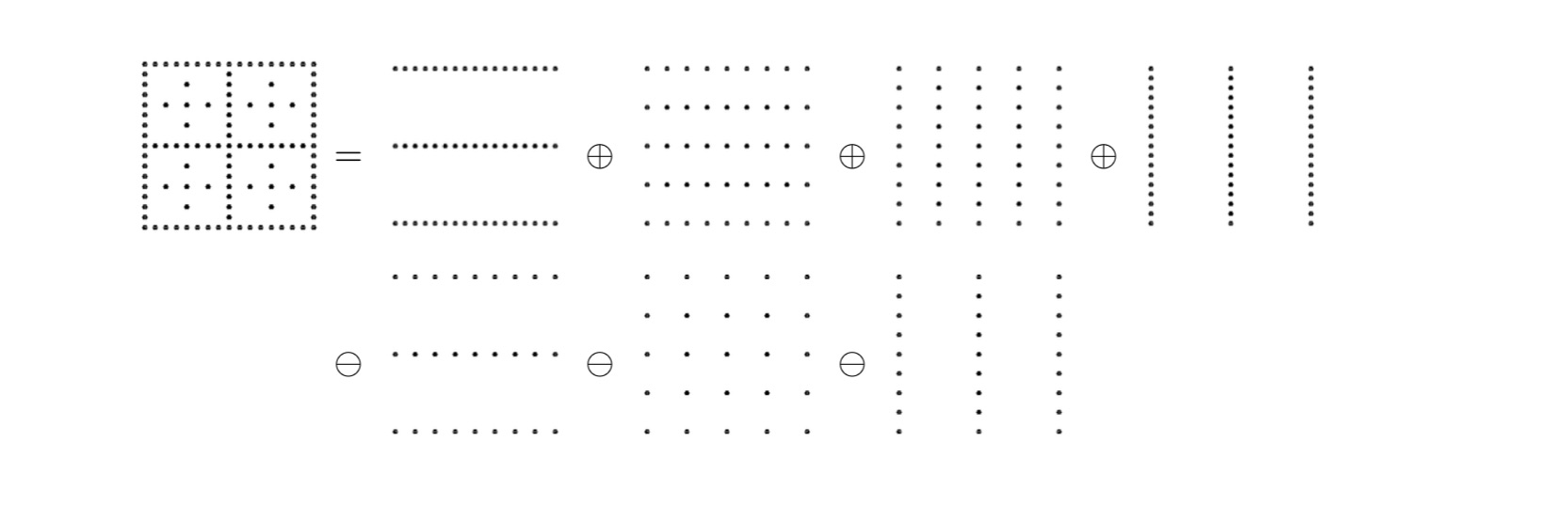
Refer to caption
Figure 2: The sparse grid 𝒮4,2\mathcal{S}_{4,2} constructed via (3.3)

Following (2.1) we represent the anisotropic convolution approximation on 𝒳ℓ\mathcal{X}_{{\bf{\ell}}} as

𝒞ℓ​(f)​(x)\displaystyle\mathcal{C}_{\boldsymbol{\ell}}(f)(\textbf{x}) =f∗Ψ(12ℓ1,…,12ℓd)​(x)=∑k∈𝐙df^​(k)​(∏i=1dψ^​(ki2ℓi))​ek​(x).\displaystyle=f\ast\Psi_{\left(\frac{1}{2^{\ell_{1}}},\ldots,\frac{1}{2^{\ell_{d}}}\right)}(\textbf{x})=\sum_{\textbf{k}\in{{\mathbf{Z}}}^{d}}\widehat{f}(\textbf{k})\left(\prod_{i=1}^{d}\widehat{\psi}\left(\frac{k_{i}}{2^{\ell_{i}}}\right)\right)e_{\textbf{k}}(\textbf{x}). (3.4)

The convolution approximation on the sparse grid 𝒮n,d\mathcal{S}_{n,d} makes use of the Boolean decomposition (3.3) and, by what is commonly called the combination technique [7], we define

𝒞n,d​(f)​(x)=∑q=0d−1(−1)q​(d−1q)​∑|ℓ|1=n+(d−1)−q𝒞ℓ​(f)​(x).{{\mathcal{C}_{n,d}(f)(\textbf{x})=\sum_{q=0}^{d-1}(-1)^{q}{d-1\choose q}\sum_{|\boldsymbol{\ell}|_{1}=n+(d-1)-q}\mathcal{C}_{\boldsymbol{\ell}}(f)(\textbf{x}).}} (3.5)

Substituting (3.4) into the above one can show that

𝒞n,d​(f)​(x)=∑k∈𝐙df^​(k)​𝒞n,d^​(k)​ek​(x)\mathcal{C}_{n,d}(f)(\textbf{x})=\sum_{\textbf{k}\in{{\mathbf{Z}}}^{d}}\widehat{f}(\textbf{k})\widehat{\mathcal{C}_{n,d}}(\textbf{k})e_{\textbf{k}}(\textbf{x})

where

𝒞n,d^(k)=(−1)d−1∑q=0d−1(−1)q(d−1q)∑|ℓ|1=n+qe−∑i=1d2​π2​ki222​ℓi.{{\widehat{\mathcal{C}_{n,d}}(\textbf{k})=(-1)^{d-1}\sum_{q=0}^{d-1}(-1)^{q}{d-1\choose q}\sum_{|\boldsymbol{\ell}|_{1}=n+q}e^{-\sum_{i=1}^{d}\frac{2\pi^{2}k_{i}^{2}}{2^{2\ell_{i}}}}.}} (3.6)

Using this representation the pointwise error formula is given by

En,d​(f)​(𝐱)=f⁡(𝐱)−𝒞n,d​(f)​(x)=∑k∈𝐙df^​(k)​ℰn,d^​(k)​ek​(x),{{E_{n,d}(f)({\bf{x}})=f({\bf{x}})-\mathcal{C}_{n,d}(f)(\textbf{x})=\sum_{\textbf{k}\in{{\mathbf{Z}}}^{d}}\widehat{f}(\textbf{k})\widehat{\mathcal{E}_{n,d}}(\textbf{k})e_{\textbf{k}}(\textbf{x}),}} (3.7)

where

ℰn,d^(k)=1−(−1)d−1∑q=0d−1(−1)q(d−1q)∑|ℓ|1=n+qe−∑i=1d2​π2​ki222​ℓi.{{\widehat{\mathcal{E}_{n,d}}(\textbf{k})=1-(-1)^{d-1}\sum_{q=0}^{d-1}(-1)^{q}{d-1\choose q}\sum_{|\boldsymbol{\ell}|_{1}=n+q}e^{-\sum_{i=1}^{d}\frac{2\pi^{2}k_{i}^{2}}{2^{2\ell_{i}}}}.}} (3.8)

We notice that when 𝐤=𝟎\bf{k}=\bf{0} we have that

ℰn,d^​(0)\displaystyle\widehat{\mathcal{E}_{n,d}}(\textbf{0}) =1−(−1)d−1​∑q=0d−1(−1)q​(d−1q)​∑|ℓ|1=n+q1\displaystyle=1-(-1)^{d-1}\sum_{q=0}^{d-1}(-1)^{q}{d-1\choose q}\sum_{|\boldsymbol{\ell}|_{1}=n+q}1 (3.9)
=1−(−1)d−1​∑q=0d−1(−1)q​(d−1q)​(n+q−1d−1),\displaystyle=1-(-1)^{d-1}\sum_{q=0}^{d-1}(-1)^{q}{d-1\choose q}{n+q-1\choose d-1},

where we have used the fact that that the number of ways to write ss as the sum of rr positive integers is (s−1r−1).{s-1\choose r-1}. The following identity, which is taken from [10] Formula 4.2.5.47, is valid for non-negative integers rr and ss such that 0≤r≤s0\leq r\leq s

∑q=0s(−1)q​(sq)​(a+b​qr)=(−1)s​bs​δr,s.\sum_{q=0}^{s}(-1)^{q}{s\choose q}{a+bq\choose r}=(-1)^{s}b^{s}\delta_{r,s}.

Applying this with r=s=d−1,r=s=d-1, a=n−1a=n-1 and b=1b=1 we can conclude that the sum in the expression above equates to (−1)d−1(-1)^{d-1} and hence we have that ℰn,d^​(0)=0.\widehat{\mathcal{E}_{n,d}}(\textbf{0})=0. Thus, as with the plain convolution approximation, the combination convolution approximation on the sparse grid also reproduces the constant function. At this point in the paper it is pertinent to compare the two error representations for convolution approximation that we have developed so far, in the continuous (full grid) setting we have

En,d​(f)​(𝐱)=f⁡(𝐱)−𝒞12n​(f)​(x)=∑𝐤∈𝐙d∖{𝟎}f^​(k)​(1−e−2​π2​‖𝐤‖222​n)​ek​(x)E_{n,d}(f)({\bf{x}})=f({\bf{x}})-\mathcal{C}_{\frac{1}{2^{n}}}(f)(\textbf{x})=\sum_{{\bf{k}}\in{{\mathbf{Z}}}^{d}\setminus\{{\bf{0}}\}}\widehat{f}(\textbf{k})\left(1-e^{-\frac{2\pi^{2}\|{\bf{k}}\|^{2}}{2^{2n}}}\right)e_{\textbf{k}}(\textbf{x})

and in the sparse grid case we have

En,d(f)(𝐱)=f(𝐱)−𝒞n,d(f)(x)=∑𝐤∈𝐙d∖{𝟎}f^(k)(1−∑q=0d−1(−1)q+d−1(d−1q)∑|ℓ|1=n+qe−∑i=1d2​π2​ki222​ℓi)ek(x).\displaystyle E_{n,d}(f)({\bf{x}})=f({\bf{x}})-\mathcal{C}_{n,d}(f)(\textbf{x})=\sum_{{\bf{k}}\in{{\mathbf{Z}}}^{d}\setminus\{{\bf{0}}\}}\widehat{f}(\textbf{k})\left(1-\sum_{q=0}^{d-1}(-1)^{q+d-1}{d-1\choose q}\sum_{|\boldsymbol{\ell}|_{1}=n+q}e^{-\sum_{i=1}^{d}\frac{2\pi^{2}k_{i}^{2}}{2^{2\ell_{i}}}}\right)e_{\textbf{k}}(\textbf{x}).

In Section 2 we found that error bounds, for sufficiently smooth functions, in the full grid case are easy to access by applying the simple inequality 1−e−x≤x.1-e^{-x}\leq x. The situation for the sparse grid case is clearly not as straightforward and this leads us to embark on a thorough investigation of the coefficients (3.8). To this end we will begin with a detailed examination of the 2−2-dimensional case. The findings from the 2−d2-d investigation will form the base case of an inductive proof which we will use to establish convergence in higher dimensions.

3.1 Convergence in two-dimensions

In two dimensions the sparse grid convolution coefficients (3.8) have the form

ℰn,2^​(k)\displaystyle\widehat{\mathcal{E}_{n,2}}(\textbf{k}) =1+∑i+j=ne−2​π2​(k1222​i+k2222​j)−∑i+j=n+1e−2​π2​(k1222​i+k2222​j).\displaystyle=1+\sum_{i+j=n}e^{-2\pi^{2}\left(\frac{k_{1}^{2}}{2^{2i}}+\frac{k_{2}^{2}}{2^{2j}}\right)}-\sum_{i+j=n+1}e^{-2\pi^{2}\left(\frac{k_{1}^{2}}{2^{2i}}+\frac{k_{2}^{2}}{2^{2j}}\right)}. (3.10)

Let us develop the general term in the above expression using the full series expansion of the exponential function. Specifically, we consider

∑i+j=me−2​π2​(k1222​i+k2222​j)\displaystyle\sum_{i+j=m}e^{-2\pi^{2}\left(\frac{k_{1}^{2}}{2^{2i}}+\frac{k_{2}^{2}}{2^{2j}}\right)} =∑i+j=m∑p=0∞(−1)p​2p​π2​pp!​(k1222​i+k2222​j)p=∑p=0∞(−1)p​2p​π2​pp!​σ2,p​(m,k),\displaystyle=\sum_{i+j=m}\sum_{p=0}^{\infty}(-1)^{p}\frac{2^{p}\pi^{2p}}{p!}\left(\frac{k_{1}^{2}}{2^{2i}}+\frac{k_{2}^{2}}{2^{2j}}\right)^{p}=\sum_{p=0}^{\infty}(-1)^{p}\frac{2^{p}\pi^{2p}}{p!}\sigma_{2,p}(m,\textbf{k}), (3.11)

where

σ2,p​(m,k)=∑i+j=m(k1222​i+k2222​j)p=∑j=1m−1(k1222​(m−j)+k2222​j)p.{{\sigma_{2,p}(m,\textbf{k})=\sum_{i+j=m}\left(\frac{k_{1}^{2}}{2^{2i}}+\frac{k_{2}^{2}}{2^{2j}}\right)^{p}=\sum_{j=1}^{m-1}\left(\frac{k_{1}^{2}}{2^{2(m-j)}}+\frac{k_{2}^{2}}{2^{2j}}\right)^{p}.}} (3.12)

We note that, when p=0p=0 we have σ2,0​(m,k)=m−1.\sigma_{2,0}(m,\textbf{k})=m-1. For p≥1p\geq 1 we can apply the binomial theorem to yield

σ2,p​(m,k)=∑j=1m−1∑r=0p(pr)​k12​r22​(m−j)​r​k22​(p−r)22​j​(p−r)=∑r=0p(pr)​k12​r​k22​(p−r)22​m​r​∑j=1m−122​(2​r−p)​j.\sigma_{2,p}(m,\textbf{k})=\sum_{j=1}^{m-1}\sum_{r=0}^{p}{p\choose r}\frac{k_{1}^{2r}}{2^{2(m-j)r}}\frac{k_{2}^{2(p-r)}}{2^{2j(p-r)}}=\sum_{r=0}^{p}{p\choose r}\frac{k_{1}^{2r}k_{2}^{2(p-r)}}{2^{2mr}}\sum_{j=1}^{m-1}2^{2(2r-p)j}.

Define

Δp,2={1if​p​is​even;0otherwise,{{\Delta_{p,2}=\begin{cases}1\,\,&\,\,\textrm{if}\,\,p\,\,{\rm{is}}\,\,{\rm{even}};\\ 0\,\,&\,\,\textrm{otherwise},\end{cases}}} (3.13)

then applying the geometric sum formula

∑j=1nxj={1x−1−1​(1−xn)if​x≠1;nif​x=1.{{\sum_{j=1}^{n}x^{j}=\begin{cases}\frac{1}{x^{-1}-1}(1-x^{n})\,\,&\,\,\textrm{if}\,\,x\neq 1;\\ n\,\,&\,\,\textrm{if}\,\,x=1.\end{cases}}} (3.14)

We find that

σ2,p​(m,k)=∑r=0r≠p2p(pr)​k12​r​k22​(p−r)22​m​r​1−22​(2​r−p)​(m−1)22​(p−2​r)−1+Δp,2​(pp2)​k1p​k2p2m​p​(m−1)\displaystyle\sigma_{2,p}(m,\textbf{k})=\sum_{\begin{subarray}{c}r=0\\ r\neq\frac{p}{2}\end{subarray}}^{p}{p\choose r}\frac{k_{1}^{2r}k_{2}^{2(p-r)}}{2^{2mr}}\frac{1-2^{2(2r-p)(m-1)}}{2^{2(p-2r)}-1}+\Delta_{p,2}{p\choose\frac{p}{2}}\frac{k_{1}^{p}k_{2}^{p}}{2^{mp}}(m-1)
=∑r=0r≠p2p(pr)⁡(k12​r​k22​(p−r)22​m​r​(22​(p−2​r)−1)−k12​(p−r)​k22​r​22​(p−2​r)​(m−1)22​m​(p−r)​(22​(2​r−p)−1))+Δp,2​(pp2)​k1p​k2p2m​p​(m−1)\displaystyle=\sum_{\begin{subarray}{c}r=0\\ r\neq\frac{p}{2}\end{subarray}}^{p}{p\choose r}\left(\frac{k_{1}^{2r}k_{2}^{2(p-r)}}{2^{2mr}(2^{2(p-2r)}-1)}-\frac{k_{1}^{2(p-r)}k_{2}^{2r}2^{2(p-2r)(m-1)}}{2^{2m(p-r)}(2^{2(2r-p)}-1)}\right)+\Delta_{p,2}{p\choose\frac{p}{2}}\frac{k_{1}^{p}k_{2}^{p}}{2^{mp}}(m-1)
=∑r=0r≠p2p(pr)​k12​r​k22​(p−r)+k12​(p−r)​k22​r22​m​r​(22​(p−2​r)−1)+Δp,2​(pp2)​k1p​k2p2m​p​(m−1).\displaystyle=\sum_{\begin{subarray}{c}r=0\\ r\neq\frac{p}{2}\end{subarray}}^{p}{p\choose r}\frac{k_{1}^{2r}k_{2}^{2(p-r)}+k_{1}^{2(p-r)}k_{2}^{2r}}{2^{2mr}(2^{2(p-2r)}-1)}+\Delta_{p,2}{p\choose\frac{p}{2}}\frac{k_{1}^{p}k_{2}^{p}}{2^{mp}}(m-1).

Using the notation introduced above we can write (3.10) as

ℰn,2^​(k)=\displaystyle\widehat{\mathcal{E}_{n,2}}(\textbf{k})= ∑p=1∞(−1)p​2p​π2​pp!​(σ2,p​(n,k)−σ2,p​(n+1,k))\displaystyle\sum_{p=1}^{\infty}\frac{(-1)^{p}2^{p}\pi^{2p}}{p!}\left(\sigma_{2,p}(n,\textbf{k})-\sigma_{2,p}(n+1,\textbf{k})\right)
=\displaystyle= ∑p=1∞(−1)p​2p​π2​pp!​∑r=1r≠p2p(pr)22​n​r​(22​r−122​(p−r)−2r)​(k12​r​k22​(p−r)+k12​(p−r)​k22​r)\displaystyle\sum_{p=1}^{\infty}\frac{(-1)^{p}2^{p}\pi^{2p}}{p!}\sum_{\begin{subarray}{c}r=1\\ r\neq\frac{p}{2}\end{subarray}}^{p}\frac{{p\choose r}}{2^{2nr}}\left(\frac{2^{2r}-1}{2^{2(p-r)}-2^{r}}\right)\left(k_{1}^{2r}k_{2}^{2(p-r)}+k_{1}^{2(p-r)}k_{2}^{2r}\right)
+∑p=1∞22​p​π4​p(2​p)!(2​pp)((22​p−122​p)n22​n​p−122​n​p)k12​pk22​p.\displaystyle+\sum_{p=1}^{\infty}\frac{2^{2p}\pi^{4p}}{(2p)!}{2p\choose p}\left(\left(\frac{2^{2p}-1}{2^{2p}}\right)\frac{n}{2^{2np}}-\frac{1}{2^{2np}}\right)k_{1}^{2p}k_{2}^{2p}.

Examining the above, we observe that the term dominating the asymptotic rate of decay corresponds to the first (p=1p=1) term of the second sum, and hence we can deduce that

ℰn,2^​(k)∼22​π42!​2⋅34​n22​n​k12​k22=3​π4​k12​k22​n22​n.\widehat{\mathcal{E}_{n,2}}(\textbf{k})\sim\frac{2^{2}\pi^{4}}{2!}2\cdot\frac{3}{4}\frac{n}{2^{2n}}k_{1}^{2}k_{2}^{2}=3\pi^{4}k_{1}^{2}k_{2}^{2}\frac{n}{2^{2n}}.

3.2 Convergence in dd-dimensions

In this part we will consider the d−d-dimensional analogue of the approach from the previous subsection. We begin by defining the d−d-dimensional analogue of (3.12)

σd,p​(m,k)={(m−1d−1)if​p=0;∑|ℓ|1=m(∑i=1dki222​ℓi)pif​p≥1.{{\sigma_{d,p}(m,\textbf{k})=\begin{cases}{m-1\choose d-1}\,\,&\,\,\textrm{if}\,\,p=0;\\ \sum_{|\boldsymbol{\ell}|_{1}=m}\left(\sum_{i=1}^{d}\frac{k_{i}^{2}}{2^{2\ell_{i}}}\right)^{p}\,\,&\,\,\textrm{if}\,\,p\geq 1.\end{cases}}} (3.15)

Then, using this notation in the expansion of the exponential function, the error coefficients (3.8) can be represented as

ℰn,d​(k)=\displaystyle\mathcal{E}_{n,d}(\textbf{k})= 1−(−1)d−1​∑p=0∞(−1)p​2p​π2​pp!​∑q=0d−1(−1)q​(d−1q)​σd,p​(n+q,k)\displaystyle 1-(-1)^{d-1}\sum_{p=0}^{\infty}\frac{(-1)^{p}2^{p}\pi^{2p}}{p!}\sum_{q=0}^{d-1}(-1)^{q}{d-1\choose q}\sigma_{d,p}(n+q,\textbf{k})
=\displaystyle= 1−(−1)d−1​∑q=0d−1(−1)q​(d−1q)​(n+q−1d−1)\displaystyle 1-(-1)^{d-1}\sum_{q=0}^{d-1}(-1)^{q}{d-1\choose q}{n+q-1\choose d-1}
−∑p=1∞(−1)p​2p​π2​pp!∑q=0d−1(−1)d−1−q(d−1q)σd,p(n+q,k).\displaystyle-\sum_{p=1}^{\infty}\frac{(-1)^{p}2^{p}\pi^{2p}}{p!}\sum_{q=0}^{d-1}(-1)^{d-1-q}{d-1\choose q}\sigma_{d,p}(n+q,\textbf{k}).

We note that the penultimate line above coincides with ℰn,d​(0)\mathcal{E}_{n,d}(\textbf{0}) (3.9) which we have shown to be zero. To simplify the notation we recall the forward divided difference functional of order kk is defined by

Δk​f=∑q=0k(−1)k−q​(kq)​f​(q).\Delta^{k}f=\sum_{q=0}^{k}(-1)^{k-q}{k\choose q}f(q).

Taking k=d−1k=d-1 we can express the d−d-dimensional sparse grid convolution error coefficients as

ℰn,d(k)=−2π2Δd−1σd,1(n+⋅,k)−∑p=2∞(−1)p​2p​π2​pp!Δd−1σd,p(n+⋅,k).\mathcal{E}_{n,d}(\textbf{k})=-2\pi^{2}\Delta^{d-1}\sigma_{d,1}(n+\cdot,\textbf{k})-\sum_{p=2}^{\infty}\frac{(-1)^{p}2^{p}\pi^{2p}}{p!}\Delta^{d-1}\sigma_{d,p}(n+\cdot,\textbf{k}).

Clearly, an investigation of σd,p​(m,k)\sigma_{d,p}(m,\textbf{k}) is required in order to shed light upon the rate at which the error coefficients decay. The following result provides the insight we need.

Theorem 3.1. Let d≥2,d\geq 2, ℓ=(ℓ1,…,ℓd)T∈I​Nd\boldsymbol{\ell}=(\ell_{1},\ldots,\ell_{d})^{T}\in{\rm I}\!{\rm N}^{d} and k=(k1,…,kd)T∈𝐙d.{\textbf{k}}=(k_{1},\ldots,k_{d})^{T}\in{{\mathbf{Z}}}^{d}. Then, for m≥d,m\geq d, we have

σd,1​(m,k)=‖k‖2​(πd−2​(m)+(−1)d−1​(43)d−1​122​m),{{\sigma_{d,1}(m,\textbf{k})=\|\textbf{k}\|^{2}\left(\pi_{d-2}(m)+(-1)^{d-1}\left(\frac{4}{3}\right)^{d-1}\frac{1}{2^{2m}}\right),}} (3.16)

where πd−2​(m)\pi_{d-2}(m) is a polynomial in mm of degree d−2.d-2. Furthermore, for p≥2p\geq 2 we also have

σd,p​(m,k)=πd−2k,p​(m)+δp,d​dk12⋯kd2md−122​m+C⁡(k,p,d)​md−222​m+O⁡(md−322​m),{{\sigma_{d,p}(m,\textbf{k})=\pi_{d-2}^{\textbf{k},p}(m)+\delta_{p,d}\frac{dk_{1}^{2}\cdots k_{d}^{2}\,m^{d-1}}{2^{2m}}+\frac{C(\textbf{k},p,d)m^{d-2}}{2^{2m}}+O\left(\frac{m^{d-3}}{2^{2m}}\right),}} (3.17)

where πd−2k,p​(m)\pi_{d-2}^{\textbf{k},p}(m) is a polynomial in mm of degree d−2d-2 whose coefficients depend upon k and p.p.

The full proof of this theorem relies on some rather technical machinery and this, together with the proof, is provided in the final section of the paper. Using the expression for σ2,p​(m,k)\sigma_{2,p}(m,\textbf{k}) that was derived in the previous subsection it is easy to verify the 2−2-dimensional version of the result with constant polynomials

π0​(m)=13,and​π0k,p​(m)=k12​p+k22​p22​p−1,p≥2,\pi_{0}(m)=\frac{1}{3},\,\,{\rm{and}}\,\,\pi_{0}^{\textbf{k},p}(m)=\frac{k_{1}^{2p}+k_{2}^{2p}}{2^{2p}-1},\,\,\,p\geq 2,

and leading constants

C⁡(k,p,2)=p⁡(k12​(p−1)​k22+k12​k22​(p−1))22​(p−2)−1,p≠2.C(\textbf{k},p,2)=\frac{p\left(k_{1}^{2(p-1)}k_{2}^{2}+k_{1}^{2}k_{2}^{2(p-1)}\right)}{2^{2(p-2)}-1},\,\,p\neq 2.

The key insight from Theorem 3.2 is that, for each p,p, the σd,p​(m,k)\sigma_{d,p}(m,\textbf{k}) function can be expressed as a polynomial in mm of degree d−2d-2 plus either a constant multiple of md−2/22​mm^{d-2}/2^{2m} (when p≠dp\neq d) or dk12⋯kd2md−1/22​mdk_{1}^{2}\cdots k_{d}^{2}m^{d-1}/2^{2m} (when OPENp=d)p=d) followed by higher order terms (i.e., those decaying at a faster rate as mm grows). Given that the forward divided difference functional annihilates polynomials of degree d−2d-2 we can, after ignoring the higher order terms, deduce that

ℰn,d^​(k)=122​n\displaystyle\widehat{\mathcal{E}_{n,d}}(\textbf{k})=\frac{1}{2^{2n}} [(−1)d2π2∥k∥2∑q=0d−1(−1)d−1−q(d−1q)122​q\displaystyle\Biggl[(-1)^{d}2\pi^{2}\|\textbf{k}\|^{2}\sum_{q=0}^{d-1}(-1)^{d-1-q}{d-1\choose q}\frac{1}{2^{2q}}
−∑p=2p≠d∞(−1)p​2p​π2​p​C​(k,p,d)p!∑q=0d−1(−1)d−1−q(d−1q)(n+q)d−222​q\displaystyle-\sum_{\begin{subarray}{c}p=2\\ p\neq d\end{subarray}}^{\infty}\frac{(-1)^{p}2^{p}\pi^{2p}C(\textbf{k},p,d)}{p!}\sum_{q=0}^{d-1}(-1)^{d-1-q}{d-1\choose q}\frac{(n+q)^{d-2}}{2^{2q}}
−(−1)d2dπ2​ddk12⋯kd2d!∑q=0d−1(−1)d−1−q(d−1q)(n+q)d−122​q+O(nd−3)].\displaystyle-\frac{(-1)^{d}2^{d}\pi^{2d}dk_{1}^{2}\cdots k_{d}^{2}}{d!}\sum_{q=0}^{d-1}(-1)^{d-1-q}{d-1\choose q}\frac{(n+q)^{d-1}}{2^{2q}}+O(n^{d-3})\Biggr].

Examining the above sum we see that the asymptotic decay of the coefficients is dominated by nd−1n^{d-1} weight arising from the application of the forward divided difference operator to (n+⋅)d−1(n+\cdot\,)^{d-1} in the final sum. Thus, using the binomial identity

∑q=0d−1(−1)d−1−q​(d−1q)​xq=(−1)d−1​(1−x)d−1,\sum_{q=0}^{d-1}(-1)^{d-1-q}{d-1\choose q}x^{q}=(-1)^{d-1}(1-x)^{d-1},

with x=1/4x=1/4 we may deduce that

ℰn,d^​(k)∼2π2​dk12⋯kd2(d−1)!​(32)d−1​nd−122​n.{{\widehat{\mathcal{E}_{n,d}}(\textbf{k})\sim\frac{2\pi^{2d}k_{1}^{2}\cdots k_{d}^{2}}{(d-1)!}\left(\frac{3}{2}\right)^{d-1}\frac{n^{d-1}}{2^{2n}}.}} (3.18)

Employing this result in (3.7) we can deduce

En,d(f)(𝐱)∼2​π2​d(d−1)!(32)d−1nd−122​n∑k∈Zdf^(k)k12⋯kd2ek(x),{{E_{n,d}(f)({\bf{x}})\sim\frac{2\pi^{2d}}{(d-1)!}\left(\frac{3}{2}\right)^{d-1}\frac{n^{d-1}}{2^{2n}}\sum_{\textbf{k}\in Z^{d}}\widehat{f}(\textbf{k})k_{1}^{2}\cdots k_{d}^{2}e_{\textbf{k}}(\textbf{x}),}} (3.19)

and, more specifically, by mirroring the proof of Proposition 2.1, we can conclude the following.

Corollary 3.2. Let f∈𝒩β,f\in\mathcal{N}_{\beta}, where β>d2+2.\beta>\frac{d}{2}+2. Let 𝒞12n​(f)\mathcal{C}_{\frac{1}{2^{n}}}(f) denote the plain Gaussian convolution approximation (2.1) to ff on the full isotropic grid 𝒳n,d\mathcal{X}_{n,d} with spacing 1/2n1/2^{n} and 𝒞n,d​(f)\mathcal{C}_{n,d}(f) denote the combined convolution approximation to ff (3.5) on the sparse grid 𝒮n,d.\mathcal{S}_{n,d}. Then

‖𝒞12n​(f)−f‖∞≤Cd22​n​‖f‖βand‖𝒞n,d​(f)−f‖∞≤Cd​nd−122​n​‖f‖β,\|\mathcal{C}_{\frac{1}{2^{n}}}(f)-f\|_{\infty}\leq\frac{C_{d}}{2^{2n}}\|f\|_{\beta}\quad{\rm{and}}\quad\|\mathcal{C}_{n,d}(f)-f\|_{\infty}\leq\frac{C_{d}n^{d-1}}{2^{2n}}\|f\|_{\beta},

where CdC_{d} denotes a generic dimension dependent constant.

We close this section by presenting some numerical results to show how closely the Fourier coefficients of the sparse grid convolution approximation track the asymptotic formula.

Table 1: Comparison of numerically computed 2−2-d expansion coefficients ℰn,2^​(k)\widehat{\mathcal{E}_{n,2}}(\textbf{k}) with the asymptotic formula (3.18), with k=(1,1)\textbf{k}=(1,1) (left) and k=(500,700)\textbf{k}=(500,700) (right)
nn ℰn,2^​(k)\widehat{\mathcal{E}_{n,2}}(\textbf{k}) formula ℰn,2^​(k)\widehat{\mathcal{E}_{n,2}}(\textbf{k}) formula
40 8.69 (-21) 9.67 (-21) 5.19 (-10) 1.18 (-9)
80 1.52 (-44) 1.60 (-44) 1.41 (-33) 1.99 (-33)
160 2.13 (-92) 2.19 (-92) 2.31 (-81) 2.68 (-81)
320 2.02 (-188) 2.05 (-188) 2.33 (-177) 2.51 (-177)
640 8.93 (-381) 8.98 (-381) 1.06 (-369) 1.10 (-369)
Table 2: Comparison of numerically computed 3−3-d expansion coefficients ℰn,3^​(k)\widehat{\mathcal{E}_{n,3}}(\textbf{k}) with the asymptotic formula (3.18), with k=(1,1,1)\textbf{k}=(1,1,1) (left) and k=(500,700,900)\textbf{k}=(500,700,900) (right)
nn ℰn,3^​(k)\widehat{\mathcal{E}_{n,3}}(\textbf{k}) formula ℰn,3^​(k)\widehat{\mathcal{E}_{n,3}}(\textbf{k}) formula
40 1.72 (-18) 2.86 (-18) 3.54 (-2) 2.84 (-1)
80 6.65 (-42) 9.47 (-42) 4.62 (-25) 9.40 (-25)
160 1.95 (-89) 2.59 (-89) 1.69 (-72) 2.57 (-72)
320 3.80 (-185) 4.85 (-185) 3.54 (-168) 4.82 (-168)
640 3.39 (-377) 4.26 (-377) 3.27 (-360) 4.22 (-360)

4 Proof of Main Theorem

The main results stated in Theorem 3.2 are not so hard to convey. The polynomials that appear in the results arise from terms in the multinomial expansion which involve iterations of finite geometric series; some of these collapse to the sum of powers of natural numbers and, as such, introduce polynomial terms in m.m. For instance, in the 2−2-dimensional investigated in subsection 3.2, we see the finite geometric sum ∑j=1m−122​(2​r−p)\sum_{j=1}^{m-1}2^{2(2r-p)} and, in the cases where 2​r=p2r=p this collapses to ∑j=1m−11=m−1,\sum_{j=1}^{m-1}1=m-1, thus introducing a linear term in m.m. If one was to carefully examine the 3−d3-d case then further instances of such sums (leading to linear terms in mm) would arise together with double sums that collapse to ∑j=1m−2j=(m−1)​(m−2)/2,\sum_{j=1}^{m-2}j=(m-1)(m-2)/2, and these introduce a quadratic term. The pattern continues into higher dimensions. The formal proof of the result is made difficult due, in part, to the notational complexity that is involved. The first result, identity (3.16), is a surprisingly neat representation for the p=1p=1 case; we were not able to develop similar neat closed form expressions for p>2.p>2. We begin by establishing (3.16), then we will develop some technical results on weighted geometric sums that will allow us to verify (3.17). We begin with the following lemma which sheds some insight on a particular finite sum.

Lemma 4.1. Let d≥2d\geq 2 be a positive integer and m>d.m>d. Then, for a positive integer r,r, we have

∑j=1m−(d−1)(m−j−1d−2)22​j​r=pd−2​(m)+(22​r1−22​r)d−1​122​r​m,\sum_{j=1}^{m-(d-1)}\frac{{m-j-1\choose d-2}}{2^{2jr}}=p_{d-2}(m)+\left(\frac{2^{2r}}{1-2^{2r}}\right)^{d-1}\frac{1}{2^{2rm}},

where pd−2​(m)p_{d-2}(m) is a polynomial in mm of degree d−2.d-2.

Proof.

Recall the Gauss hypergeometric function (see [1], 15.1.1) is defined by

F12​(a,b,c,z):=∑j=0∞(a)j​(b)j(c)j​zjj!,{{{}_{2}F_{1}(a,b;c;z):=\sum_{j=0}^{\infty}\frac{(a)_{j}(b)_{j}}{(c)_{j}}\frac{z^{j}}{j!},}} (4.1)

where

(x)j:=x(x+1)⋯(x+j−1)j≥1{{(x)_{j}:=x(x+1)\cdots(x+j-1)\quad j\geq 1}} (4.2)

denotes the Pochhammer symbol, with (x)0=1(x)_{0}=1. If nn is a positive integer we have

(n)j=(n+j−1)!(n−1)!and(−n)j=(−1)j​n!(n−j)!.(n)_{j}=\frac{(n+j-1)!}{(n-1)!}\quad{\rm{and}}\quad(-n)_{j}=\frac{(-1)^{j}n!}{(n-j)!}.

Using the above it is straight forward to verify that

∑j=1m−(d−1)(m−j−1d−2)22​j​p=122​p​(m−2d−2)​F12​(1,−(m−d),−(m−2),122​p).{{\sum_{j=1}^{m-(d-1)}\frac{{m-j-1\choose d-2}}{2^{2jp}}=\frac{1}{2^{2p}}{m-2\choose d-2}{}_{2}F_{1}\left(1,-(m-d);-(m-2);\frac{1}{2^{2p}}\right).}} (4.3)

The following identity, see [11] Formula 7.3.1.178, is valid for non-negative integers pp and qq

F12​(1,−p,−q,z)=q+1p+1​∑k=0q−p(p−q)k(p+2)k​(1−z)−(k+1)+(−1)p​p!(−q)p​zq+1​(z−1)p−q−1.{}_{2}F_{1}(1,-p;-q;z)=\frac{q+1}{p+1}\sum_{k=0}^{q-p}\frac{(p-q)_{k}}{(p+2)_{k}}(1-z)^{-(k+1)}+\frac{(-1)^{p}p!}{(-q)_{p}}z^{q+1}(z-1)^{p-q-1}.

Applying this with p=m−d,p=m-d, q=m−2q=m-2 and z=122​r,z=\frac{1}{2^{2r}}, we find that

F12​(1,−(m−d),−(m−2),122​r)=\displaystyle{}_{2}F_{1}\left(1,-(m-d);-(m-2);\frac{1}{2^{2r}}\right)=
m−1m−(d−1)​∑k=0d−2(−(d−2))k​(22​r22​r−1)k+1(m−(d−2))k+(−1)m−1​(m−d)!​(22​r22​r−1)d−1(−(m−2))m−d​22​r22​r​m\displaystyle\frac{m-1}{m-(d-1)}\sum_{k=0}^{d-2}\frac{\left(-(d-2)\right)_{k}\left(\frac{2^{2r}}{2^{2r}-1}\right)^{k+1}}{\left(m-(d-2)\right)_{k}}+\frac{(-1)^{m-1}(m-d)!\left(\frac{2^{2r}}{2^{2r}-1}\right)^{d-1}}{\left(-(m-2)\right)_{m-d}}\frac{2^{2r}}{2^{2rm}}
=(m−1)​∑k=0d−2(−1)k​(d−2)!​(m−d)!​(22​r22​r−1)k+1(d−2−k)!​(m+k−(d−1))!+(−1)d−1​22​r​(22​r22​r−1)d−1(m−2d−2)​22​r​m.\displaystyle=(m-1)\sum_{k=0}^{d-2}\frac{(-1)^{k}(d-2)!(m-d)!\left(\frac{2^{2r}}{2^{2r}-1}\right)^{k+1}}{(d-2-k)!(m+k-(d-1))!}+\frac{(-1)^{d-1}2^{2r}\left(\frac{2^{2r}}{2^{2r}-1}\right)^{d-1}}{{m-2\choose d-2}2^{2rm}}.

In view of (4.3) we now multiply this by 122​r​(m−2d−2)\frac{1}{2^{2r}}{m-2\choose d-2} and, following some elementary simplifications, we have the following expression

∑j=1m−(d−1)(m−j−1d−2)22​r​j\displaystyle\sum_{j=1}^{m-(d-1)}\frac{{m-j-1\choose d-2}}{2^{2rj}} =∑k=0d−2(−1)k​(m−1m+k−(d−1))​(22​r22​r−1)k22​r−1+(−1)d−1​(22​r22​r−1)d−122​r​m\displaystyle=\sum_{k=0}^{d-2}\frac{(-1)^{k}{m-1\choose m+k-(d-1)}\left(\frac{2^{2r}}{2^{2r}-1}\right)^{k}}{2^{2r}-1}+\frac{(-1)^{d-1}\left(\frac{2^{2r}}{2^{2r}-1}\right)^{d-1}}{2^{2rm}}
=pd−2r​(m)+(22​r1−22​r)d−1​122​r​m,\displaystyle=p^{r}_{d-2}(m)+\left(\frac{2^{2r}}{1-2^{2r}}\right)^{d-1}\frac{1}{2^{2rm}},

where pd−2r​(m),p^{r}_{d-2}(m), which represents the sum appearing above, is a polynomial in mm of degree d−2.d-2. ∎

4.1 Proof of (3.16)

We know from (3.30)(3.30) that

σd,1​(m,k)=∑|ℓ|1=mk1222​ℓ1+⋯+kd222​ℓd=∑i=1dki2​∑|ℓ|1=m122​ℓi.\displaystyle\sigma_{d,1}(m,\textbf{k})=\sum_{|\boldsymbol{\ell}|_{1}=m}\frac{k_{1}^{2}}{2^{2\ell_{1}}}+\cdots+\frac{k_{d}^{2}}{2^{2\ell_{d}}}=\sum_{i=1}^{d}k_{i}^{2}\sum_{|\boldsymbol{\ell}|_{1}=m}\frac{1}{2^{2\ell_{i}}.}

The above sum concerns the set of d−d-dimensional multi-indices ℓ\boldsymbol{\ell} satisfying |ℓ|1=m.|\boldsymbol{\ell}|_{1}=m. A typical component ℓi\ell_{i} of ℓ\boldsymbol{\ell} can, theoretically, take on any value between 11 and m−(d−1)m-(d-1) included (in the latter case remaining d−1d-1 components are all set to OPEN1)1). The number of times ℓi\ell_{i} takes on a certain value j∈{1,2,…,m−(d−1)}j\in\{1,2,\ldots,m-(d-1)\} is precisely the number of ways in which the remaining d−1d-1 components of ℓ\boldsymbol{\ell} sum to m−jm-j and this is given by (m−j−1d−2).{m-j-1\choose d-2}. Since the last sum in the above expression only depends on the value ℓi\ell_{i} and not on ii we have that

σd,1​(m,k)\displaystyle\sigma_{d,1}(m,\textbf{k}) =∑i=1dki2​∑j=1m−(d−1)(m−j−1d−2)​122​j=‖k‖2​(pd−2​(m)+(221−22)d−1​122​m),\displaystyle=\sum_{i=1}^{d}k_{i}^{2}\sum_{j=1}^{m-(d-1)}{m-j-1\choose d-2}\frac{1}{2^{2j}}=\|\textbf{k}\|^{2}\left(p_{d-2}(m)+\left(\frac{2^{2}}{1-2^{2}}\right)^{d-1}\frac{1}{2^{2m}}\right),

where the last equation follows from Lemma 4.1, with r=1,r=1, and the proof of (3.16) is complete.

4.2 On weighted geometric sums

In this subsection we outline some key results on the representation of the kinds of weighted geometric series that are encountered if one applies the appropriate multinomial expansion in order to examine the sums σd,p​(m,𝐤)\sigma_{d,p}(m,\bf{k}) (3.15) for p≥2.p\geq 2. We begin by differentiating the plain geometric sum formula, followed by multiplication by xx to deduce that

∑j=1nj​xj=x​dd​x​∑j=1nxj={x(1−x)2​(1−xn​((1+n)−n​x))if​x≠1;∑k=1nk=n⁡(n+1)2if​x=1.{{\sum_{j=1}^{n}jx^{j}=x\frac{d}{dx}\sum_{j=1}^{n}x^{j}=\begin{cases}\frac{x}{(1-x)^{2}}\left(1-x^{n}\left((1+n)-nx\right)\right)\,\,&\,\,{\textrm{if}}\,\,\,\,x\neq 1;\\ \sum_{k=1}^{n}k=\frac{n(n+1)}{2}\,\,&\,\,{\textrm{if}}\,\,\,\,x=1.\end{cases}}} (4.4)

Let us consider the more general weighted geometric sum

Gi(n)​(x)=∑j=1nji​xj.G_{i}^{(n)}(x)=\sum_{j=1}^{n}j^{i}x^{j}.

We note in the case where x=1x=1 we have the sum of the it​hi^{th} powers of the first nn positive integers which, due to Faulhaber’s formula, see [6] Formula 0.121, is a polynomial in nn of degree i+1,i+1,

Gi(n)​(1)=∑j=1nji=ni+1i+1+qi​(n),{{G_{i}^{(n)}(1)=\sum_{j=1}^{n}j^{i}=\frac{n^{i+1}}{i+1}+q_{i}(n),}} (4.5)

where qi​(n)q_{i}(n) is a polynomial in nn of degree i.i. For the more general case (x≠1x\neq 1) we observe that

Gi+1(n)​(x)=x​dd​x​Gi(n)​(x){{G_{i+1}^{(n)}(x)=x\frac{d}{dx}G_{i}^{(n)}(x)}} (4.6)

and this allows us to establish the following.

Lemma 4.2. Let jj denote a non-negative integer and x≠1,x\neq 1, then

Gi(n)​(x)=x(1−x)i+1​(qi−1​(x)−xn​pi​(x,n)),{{G_{i}^{(n)}(x)=\frac{x}{(1-x)^{i+1}}\left(q_{i-1}(x)-x^{n}p_{i}(x,n)\right),}} (4.7)

where qi−1​(x)q_{i-1}(x) is a polynomial of degree i−1i-1 in xx and pi​(x,n)p_{i}(x,n) is a polynomial of degree ii in both xx and n.n.

Proof.

We establish the result via induction. Appealing to (4.4) we see that the result is true for i=1i=1 with q0​(x)=1q_{0}(x)=1 and p1​(x,n)=1+n−n​x.p_{1}(x,n)=1+n-nx. Assume the result is true for ii and consider the following development, using (4.6), for the case i+1.i+1.

Gi+1(n)​(x)\displaystyle G_{i+1}^{(n)}(x) =x​dd​x​Gi(n)​(x)=x​dd​x​(x(1−x)i+1​(qi−1​(x)−xn​pi​(x,n)))\displaystyle=x\frac{d}{dx}G_{i}^{(n)}(x)=x\frac{d}{dx}\left(\frac{x}{(1-x)^{i+1}}\left(q_{i-1}(x)-x^{n}p_{i}(x,n)\right)\right)
=x[x(1−x)i+1(dd​xqi−1(x)−xndd​xpi(x,n)−nxn−1pi(x,n))\displaystyle=x\Bigl[\frac{x}{(1-x)^{i+1}}\left(\frac{d}{dx}q_{i-1}(x)-x^{n}\frac{d}{dx}p_{i}(x,n)-nx^{n-1}p_{i}(x,n)\right)
+(1(1−x)i+1+i​x+x(1−x)i+2)(qi−1(x)−xnpi(x,n))]\displaystyle+\left(\frac{1}{(1-x)^{i+1}}+\frac{ix+x}{(1-x)^{i+2}}\right)\left(q_{i-1}(x)-x^{n}p_{i}(x,n)\right)\Bigr]
=x(1−x)i+2[x(1−x)(dd​xqi−1(x)−xndd​xpi(x,n)−nxn−1pi(x,n))\displaystyle=\frac{x}{(1-x)^{i+2}}\Bigl[x(1-x)\left(\frac{d}{dx}q_{i-1}(x)-x^{n}\frac{d}{dx}p_{i}(x,n)-nx^{n-1}p_{i}(x,n)\right)
+(1+ix)(qi−1(x)−xnpi(x,n))]\displaystyle+(1+ix)\left(q_{i-1}(x)-x^{n}p_{i}(x,n)\right)\Bigr]
=x(1−x)i+2​[qi​(x)−xn​pi+1​(x,n)],\displaystyle=\frac{x}{(1-x)^{i+2}}\Bigl[q_{i}(x)-x^{n}p_{i+1}(x,n)\Bigr],

where

qi​(x)=(1+i​x)​qi−1​(x)+x⁡(1−x)​dd​x​qi−1​(x)q_{i}(x)=(1+ix)q_{i-1}(x)+x(1-x)\frac{d}{dx}q_{i-1}(x)

is clearly a polynomial in xx of degree ii and, likewise, where

pi+1​(x,n)=(1+i​x+n−n​x)​pi​(x,n)+x⁡(1−x)​dd​x​pi​(x,n)p_{i+1}(x,n)=(1+ix+n-nx)p_{i}(x,n)+x(1-x)\frac{d}{dx}p_{i}(x,n)

is clearly a polynomial of degree i+1i+1 in both xx and n.n.

∎

In order to prepare for how the above result will be used, we let dd be the fixed spatial dimension and m>dm>d a positive integer. In what follows we will evaluate various sums and, in each case, we will ignore terms that decay faster than md−2​2−2​mm^{d-2}2^{-2m} for large m.m. In each case we consider a fixed integer parameter t≥1t\geq 1 and, where appropriate, we will also consider specific cases of t=0t=0 and t=−1.t=-1. We begin with a straightforward geometric sum for t≥1t\geq 1

∑j=1m−d122​j​t=122​t−1​(1−22​d​t22​m​t)=constant+O⁡(2−2​m).{{\sum_{j=1}^{m-d}\frac{1}{2^{2jt}}=\frac{1}{2^{2t}-1}\left(1-\frac{2^{2dt}}{2^{2mt}}\right)={\rm{constant}}+O(2^{-2m}).}} (4.8)

For the following sum with t>1t>1 we can directly use (4.7) in its evaluation:

∑j=1m−d(m−j)i22​t​j\displaystyle\sum_{j=1}^{m-d}\frac{(m-j)^{i}}{2^{2tj}} =122​m​t​∑j=dm−122​t​j​ji=122​m​t​(Gi(m−1)​(22​t)−Gi(d−1)​(22​t))\displaystyle=\frac{1}{2^{2mt}}\sum_{j=d}^{m-1}2^{2tj}j^{i}=\frac{1}{2^{2mt}}\left(G_{i}^{(m-1)}(2^{2t})-G_{i}^{(d-1)}(2^{2t})\right) (4.9)
=1(1−22​t)i+1​[22​t​d22​t​m​pi​(22​t,d−1)−pi​(22​t,m−1)]\displaystyle=\frac{1}{(1-2^{2t})^{i+1}}\Bigl[\frac{2^{2td}}{2^{2tm}}p_{i}(2^{2t},d-1)-p_{i}(2^{2t},m-1)\Bigr]
=Pi​(m)(1−22​t)i+1+O⁡(2−2​m),\displaystyle=\frac{P_{i}(m)}{(1-2^{2t})^{i+1}}+O(2^{-2m}),

where Pi​(m)P_{i}(m) is a polynomial in mm of degree ii whose coefficients depend on 22​t.2^{2t}. In the case where t=0t=0 the above collapses to

∑j=1m−d(m−j)i\displaystyle\sum_{j=1}^{m-d}(m-j)^{i} =∑j=dm−dji=Gim−1​(1)−Gid−1​(1)\displaystyle=\sum_{j=d}^{m-d}j^{i}=G_{i}^{m-1}(1)-G_{i}^{d-1}(1) (4.10)
=(m−1)i+1i+1−(d−1)i+1i+1+qi​(0,d−1)−qi​(0,m−1)\displaystyle=\frac{(m-1)^{i+1}}{i+1}-\frac{(d-1)^{i+1}}{i+1}+q_{i}(0,d-1)-q_{i}(0,m-1)
=mi+1i+1+πi​(m),\displaystyle=\frac{m^{i+1}}{i+1}+\pi_{i}(m),

where πi​(m)\pi_{i}(m) is a polynomial in mm of degree i.i. In the case where t=−1t=-1 we have

∑j=1m−d22​j​(m−j)i=Cd,i​22​m+(43)i+1​Pi∗​(m){{\sum_{j=1}^{m-d}2^{2j}(m-j)^{i}=C_{d,i}2^{2m}+\left(\frac{4}{3}\right)^{i+1}P^{*}_{i}(m)}} (4.11)

where Pi∗​(m)P^{*}_{i}(m) is a polynomial in mm of degree ii and Cd,iC_{d,i} is a constant depending on dd and i.i.

4.3 Proof of (3.17)

We know from subsection 3.1. that (3.17) holds for d=2d=2 and any value pp, let us also assume that it is true for d0<dd_{0}<d and any value of p,p, we will now proceed to show, by induction, that the same statement is true for dd and any value of p.p. First we establish a recurrence relation for σd,p\sigma_{d,p} using 𝒓=(r1,…,rd)T\boldsymbol{r}=(r_{1},\ldots,r_{d})^{T}, 𝒓^=(r1,…,rd−1)T\hat{\boldsymbol{r}}=(r_{1},\ldots,r_{d-1})^{T}, ℓ^=(ℓ1,…,ℓd−1)T\hat{\boldsymbol{\ell}}=(\ell_{1},\ldots,\ell_{d-1})^{T}, 𝒌^=(k1,…,kd−1)T\hat{\boldsymbol{k}}=(k_{1},\ldots,k_{d-1})^{T} and the multinomial theorem to find

σd,p​(m,k)=∑|ℓ|1=m(∑i=1dki222​ℓi)p\displaystyle\sigma_{d,p}(m,\textbf{k})=\sum_{|\boldsymbol{\ell}|_{1}=m}\left(\sum_{i=1}^{d}\frac{k_{i}^{2}}{2^{2\ell_{i}}}\right)^{p}
=∑|ℓ|1=m∑|r|=p(pr1​…​rd)∏i=1d(ki222​ℓi)ri( multinomial theorem)\displaystyle=\sum_{|\boldsymbol{\ell}|_{1}=m}\sum_{|r|=p}{p\choose r_{1}\ \ldots\ r_{d}}\prod_{i=1}^{d}\left(\frac{k_{i}^{2}}{2^{2\ell_{i}}}\right)^{r_{i}}\quad\text{( multinomial theorem)}
=∑|𝒓|=p(pr1​…​rd)∏i=1dki2​ri∑|ℓ|1=m(2∑i=1d−2ℓiri)\displaystyle=\sum_{|\boldsymbol{r}|=p}{p\choose r_{1}\ \ldots\ r_{d}}\prod_{i=1}^{d}k_{i}^{2r_{i}}\sum_{|\boldsymbol{\ell}|_{1}=m}\left(2^{\sum_{i=1}^{d}-2\ell_{i}r_{i}}\right)
=∑rd=0pp!​kd2​rd(p−rd)!​rd!∑ℓd=1m−d2−2​ℓd​rd∑|𝒓^|=p−rd(p−rdr1​…​rd−1)∏i=1d−1ki2​ri∑|ℓ^|1=m−ℓd(2∑i=1d−2ℓiri)\displaystyle=\sum_{r_{d}=0}^{p}\frac{p!k_{d}^{2r_{d}}}{(p-r_{d})!r_{d}!}\sum_{\ell_{d}=1}^{m-d}2^{-2\ell_{d}r_{d}}\sum_{|\hat{\boldsymbol{r}}|=p-r_{d}}{p-r_{d}\choose r_{1}\ \ldots\ r_{d-1}}\prod_{i=1}^{d-1}k_{i}^{2r_{i}}\sum_{|\hat{\boldsymbol{\ell}}|_{1}=m-\ell_{d}}\left(2^{\sum_{i=1}^{d}-2\ell_{i}r_{i}}\right)
=∑rd=0pp!​kd2​rd(p−rd)!​rd!​∑ℓd=1m−dσd−1,p−rd​(m−ℓd,𝒌^)22​ℓd​rd.\displaystyle=\sum_{r_{d}=0}^{p}\frac{p!k_{d}^{2r_{d}}}{(p-r_{d})!r_{d}!}\sum_{\ell_{d}=1}^{m-d}\frac{\sigma_{d-1,p-r_{d}}(m-\ell_{d},\hat{\boldsymbol{k}})}{2^{2\ell_{d}r_{d}}}.

Applying the inductive hypothesis (3.17) we have

σd−1,p−rd​(m−ℓd,𝒌^)=\displaystyle\sigma_{d-1,p-r_{d}}(m-\ell_{d},\hat{\boldsymbol{k}})= πd−3𝒌^,p−rd​(m−ℓd)+δp−rd,d−1​(d−1)k12⋯kd−12(m−ℓd)d−222​(m−ℓd)\displaystyle\pi_{d-3}^{\hat{\boldsymbol{k}},p-r_{d}}(m-\ell_{d})+\delta_{p-r_{d},d-1}\frac{(d-1)k_{1}^{2}\cdots k_{d-1}^{2}(m-\ell_{d})^{d-2}}{2^{2(m-\ell_{d})}}
+C⁡(𝒌^,p−rd,d−1)​(m−ℓd)d−322​(m−ℓd)+O⁡(md−422​m).\displaystyle+C(\hat{\boldsymbol{k}},p-r_{d},d-1)\frac{(m-\ell_{d})^{d-3}}{2^{2(m-\ell_{d})}}+O\left(\frac{m^{d-4}}{2^{2m}}\right).

Inserting this representation into the inner sum of the above computation yields

∑ℓd=1m−dσd−1,p−rd​(m−ℓd,𝒌^)22​ℓd​rd=S1​(rd)+S2​(rd)+S3​(rd)+O⁡(md−322​m),{{\sum_{\ell_{d}=1}^{m-d}\frac{\sigma_{d-1,p-r_{d}}(m-\ell_{d},\hat{\boldsymbol{k}})}{2^{2\ell_{d}r_{d}}}=S_{1}(r_{d})+S_{2}(r_{d})+S_{3}(r_{d})+O\left(\frac{m^{d-3}}{2^{2m}}\right),}} (4.12)

where

S1​(rd)\displaystyle S_{1}(r_{d}) =∑ℓd=1m−dπd−3𝒌^,p−rd​(m−ℓd)22​ℓd​rd,\displaystyle=\sum_{\ell_{d}=1}^{m-d}\frac{\pi_{d-3}^{\hat{\boldsymbol{k}},p-r_{d}}(m-\ell_{d})}{2^{2\ell_{d}r_{d}}}, (4.13)
S2​(rd)\displaystyle S_{2}(r_{d}) =δp−rd,d−1​(d−1)​k12⋯kd−1222​m​∑ℓd=1m−d(m−ℓd)d−222​ℓd​(rd−1),\displaystyle=\delta_{p-r_{d},d-1}(d-1)\frac{k_{1}^{2}\cdots k_{d-1}^{2}}{2^{2m}}\sum_{\ell_{d}=1}^{m-d}\frac{(m-\ell_{d})^{d-2}}{2^{2\ell_{d}(r_{d}-1)}},
andS3​(rd)\displaystyle{\rm{and}}\quad S_{3}(r_{d}) =C⁡(𝒌^,p−rd,d−1)22​m​∑ℓd=1m−d(m−ℓd)d−322​ℓd​(rd−1).\displaystyle=\frac{C(\hat{\boldsymbol{k}},p-r_{d},d-1)}{2^{2m}}\sum_{\ell_{d}=1}^{m-d}\frac{(m-\ell_{d})^{d-3}}{2^{2\ell_{d}(r_{d}-1)}}.

For the final term of (4.12) we have used that the sum consists of less than mm terms and each of which is order md−422​m\frac{m^{d-4}}{2^{2m}}. We can use the weighted geometric sums to investigate the three summands above. We begin with S1​(rd)S_{1}(r_{d}) and in this case we write the polynomial of degree d−3d-3 as

πd−3𝒌^,p−rd​(m−ℓd)=∑i=0d−3ai𝒌^,p−rd​(m−ℓd)i,\pi_{d-3}^{\hat{\boldsymbol{k}},p-r_{d}}(m-\ell_{d})=\sum_{i=0}^{d-3}a_{i}^{\hat{\boldsymbol{k}},p-r_{d}}(m-\ell_{d})^{i},

and thus we have

S1​(rd)=∑i=1d−3ai𝒌^,p−rd​∑ℓd=1m−d(m−ℓd)i22​ℓd​rd.S_{1}(r_{d})=\sum_{i=1}^{d-3}a_{i}^{\hat{\boldsymbol{k}},p-r_{d}}\sum_{\ell_{d}=1}^{m-d}\frac{(m-\ell_{d})^{i}}{2^{2\ell_{d}r_{d}}}.

Appealing to (4.9) and (4.10) we have that

∑ℓd=1m−d(m−ℓd)i22​ℓd​rd={Pi​(m)(1−22​rd)i+1+O⁡(2−2​m)ifrd≠0;mi+1i+1+πi​(m)ifrd=0,\sum_{\ell_{d}=1}^{m-d}\frac{(m-\ell_{d})^{i}}{2^{2\ell_{d}r_{d}}}=\begin{cases}\frac{P_{i}(m)}{(1-2^{2r_{d}})^{i+1}}+O(2^{-2m})\quad&{\rm{if}}\quad r_{d}\neq 0;\\ \frac{m^{i+1}}{i+1}+\pi_{i}(m)\quad&{\rm{if}}\quad r_{d}=0,\end{cases}

where Pi​(m)P_{i}(m) and πi​(m)\pi_{i}(m) are polynomials in mm of degree i.i. This insight allows us to write

S1​(rd)={Pd−3𝒌^,p,rd​(m)+O⁡(122​m)ifrd≠0;Pd−2𝒌^,p,0​(m)ifrd=0,{{S_{1}(r_{d})=\begin{cases}P_{d-3}^{\hat{\boldsymbol{k}},p,r_{d}}(m)+O\left(\frac{1}{2^{2m}}\right)\quad&{\rm{if}}\quad r_{d}\neq 0;\\ P_{d-2}^{\hat{\boldsymbol{k}},p,0}(m)\quad&{\rm{if}}\quad r_{d}=0,\end{cases}}} (4.14)

where

Pd−3𝒌^,p,rd​(m)=∑i=1d−3ai𝒌^,p−rd(1−22​rd)i+1​Pi​(m)andPd−2𝒌^,p,0​(m)=∑i=1d−3ai𝒌^,p​(mi+1i+1+πi​(m)){{P_{d-3}^{\hat{\boldsymbol{k}},p,r_{d}}(m)=\sum_{i=1}^{d-3}\frac{a_{i}^{\hat{\boldsymbol{k}},p-r_{d}}}{(1-2^{2r_{d}})^{i+1}}P_{i}(m)\quad{\rm{and}}\quad P_{d-2}^{\hat{\boldsymbol{k}},p,0}(m)=\sum_{i=1}^{d-3}a_{i}^{\hat{\boldsymbol{k}},p}\left(\frac{m^{i+1}}{i+1}+\pi_{i}(m)\right)}} (4.15)

are polynomials in mm of degree d−3d-3 and d−2d-2 respectively.

For the second sum S2​(rd)S_{2}(r_{d}) we can bring the identities (4.9), (4.10) and (4.11) together to give

∑ℓd=1m−d(m−ℓd)d−222​ℓd​(rd−1)={Pd−2​(m)(1−22​(rd−1))d−1+O⁡(2−2​m)ifrd>1;md−1d−1+πd−2​(m)ifrd=1;Cd,d−2​22​m+(43)d−1​Pd−2∗​(m)ifrd=0,\sum_{\ell_{d}=1}^{m-d}\frac{(m-\ell_{d})^{d-2}}{2^{2\ell_{d}(r_{d}-1)}}=\begin{cases}\frac{P_{d-2}(m)}{(1-2^{2(r_{d}-1)})^{d-1}}+O(2^{-2m})\quad&{\rm{if}}\quad r_{d}>1;\\ \frac{m^{d-1}}{d-1}+\pi_{d-2}(m)\quad&{\rm{if}}\quad r_{d}=1;\\ C_{d,d-2}2^{2m}+\left(\frac{4}{3}\right)^{d-1}P_{d-2}^{*}(m)\quad&{\rm{if}}\quad r_{d}=0,\end{cases}

and so deduce that

S2(rd)=δp−rd,d−1(d−1)(k12⋯kd−12){Pd−2​(m)22​m​(1−22​(rd−1))d−1+O⁡(2−4​m)ifrd>1;md−122​m​(d−1)+πd−2​(m)22​mifrd=1;Cd,d−2+(43)d−1​Pd−2∗​(m)22​mifrd=0.S_{2}(r_{d})=\delta_{p-r_{d},d-1}(d-1)\left(k_{1}^{2}\cdots k_{d-1}^{2}\right)\begin{cases}\frac{P_{d-2}(m)}{2^{2m}(1-2^{2(r_{d}-1)})^{d-1}}+O(2^{-4m})\quad&{\rm{if}}\quad r_{d}>1;\\ \frac{m^{d-1}}{2^{2m}(d-1)}+\frac{\pi_{d-2}(m)}{2^{2m}}\quad&{\rm{if}}\quad r_{d}=1;\\ C_{d,d-2}+\left(\frac{4}{3}\right)^{d-1}\frac{P_{d-2}^{*}(m)}{2^{2m}}\quad&{\rm{if}}\quad r_{d}=0.\end{cases}

Isolating the dominant term from those exhibiting faster decay we have that

S2(rd)=δp−rd,d−1(k12⋯kd−12){Cd​md−222​m+O⁡(md−322​m)ifrd>1;md−122​m+O⁡(md−222​m)ifrd=1;Cd′+O⁡(md−222​m)ifrd=0,{{S_{2}(r_{d})=\delta_{p-r_{d},d-1}\left(k_{1}^{2}\cdots k_{d-1}^{2}\right)\begin{cases}\frac{C_{d}m^{d-2}}{2^{2m}}+O\left(\frac{m^{d-3}}{2^{2m}}\right)\quad&{\rm{if}}\quad r_{d}>1;\\ \frac{m^{d-1}}{2^{2m}}+O\left(\frac{m^{d-2}}{2^{2m}}\right)\quad&{\rm{if}}\quad r_{d}=1;\\ C_{d}^{\prime}+O\left(\frac{m^{d-2}}{2^{2m}}\right)\quad&{\rm{if}}\quad r_{d}=0,\end{cases}}} (4.16)

where Cd′=(d−1)​Cd,d−2.C_{d}^{\prime}=(d-1)C_{d,d-2}. For the third sum S3​(rd)S_{3}(r_{d}) we can use the same approach as above, with d−3d-3 replacing d−2,d-2, to deduce that

S3​(rd)=C⁡(𝒌^,p−rd,d−1)​{Cd−1​md−322​m+O⁡(md−422​m)ifrd>1;md−2(d−2)​22​m+O⁡(md−322​m)ifrd=1;Cd−1′+O⁡(md−322​m)ifrd=0.{{S_{3}(r_{d})=C(\hat{\boldsymbol{k}},p-r_{d},d-1)\begin{cases}\frac{C_{d-1}m^{d-3}}{2^{2m}}+O\left(\frac{m^{d-4}}{2^{2m}}\right)\quad&{\rm{if}}\quad r_{d}>1;\\ \frac{m^{d-2}}{(d-2)2^{2m}}+O\left(\frac{m^{d-3}}{2^{2m}}\right)\quad&{\rm{if}}\quad r_{d}=1;\\ C_{d-1}^{\prime}+O\left(\frac{m^{d-3}}{2^{2m}}\right)\quad&{\rm{if}}\quad r_{d}=0.\end{cases}}} (4.17)

We now bring our findings (4.14),(4.16),(4.17) together, where again we isolate the dominant terms from those with faster decay to provide

σd,p​(m,𝒌)\displaystyle\sigma_{d,p}(m,\boldsymbol{k}) =∑rd=0pp!​kd2​rd(p−rd)!​rd!​(S1​(rd)+S2​(rd)+S3​(rd))+O⁡(md−322​m)\displaystyle=\sum_{r_{d}=0}^{p}\frac{p!k_{d}^{2r_{d}}}{(p-r_{d})!r_{d}!}\left(S_{1}(r_{d})+S_{2}(r_{d})+S_{3}(r_{d})\right)+O\left(\frac{m^{d-3}}{2^{2m}}\right)
=Pd−2𝒌^,p,0​(m)+∑rd=1pp!​kd2​rd(p−rd)!​rd!​Pd−3𝒌^,p,rd​(m)\displaystyle=P_{d-2}^{\hat{\boldsymbol{k}},p,0}(m)+\sum_{r_{d}=1}^{p}\frac{p!k_{d}^{2r_{d}}}{(p-r_{d})!r_{d}!}P_{d-3}^{\hat{\boldsymbol{k}},p,r_{d}}(m)
+δp,d−1(k12⋯kd−12)Cd′+δp−1,d−1(k12⋯kd−12)kd2​p!(p−1)!md−122​m+O(md−222​m)\displaystyle+\delta_{p,d-1}\left(k_{1}^{2}\cdots k_{d-1}^{2}\right)C_{d}^{\prime}+\delta_{p-1,d-1}\left(k_{1}^{2}\cdots k_{d-1}^{2}\right)\frac{k_{d}^{2}p!}{(p-1)!}\frac{m^{d-1}}{2^{2m}}+O\left(\frac{m^{d-2}}{2^{2m}}\right)
+C⁡(𝒌^,p,d−1)​Cd−1′+C⁡(𝒌^,p−1,d−1)​p​kd2d−2​md−222​m+O⁡(md−322​m).\displaystyle+C(\hat{\boldsymbol{k}},p,d-1)C_{d-1}^{\prime}+C(\hat{\boldsymbol{k}},p-1,d-1)\frac{pk_{d}^{2}}{d-2}\frac{m^{d-2}}{2^{2m}}+O\left(\frac{m^{d-3}}{2^{2m}}\right).

By inspection we observe that the above can be expressed as

σd,p​(m,k)=πd−2k,p​(m)+δp,d​dk12⋯kd2md−122​m+C⁡(k,p,d)​md−222​m+O⁡(md−322​m),{{\sigma_{d,p}(m,\textbf{k})=\pi_{d-2}^{\textbf{k},p}(m)+\delta_{p,d}\frac{dk_{1}^{2}\cdots k_{d}^{2}m^{d-1}}{2^{2m}}+\frac{C(\textbf{k},p,d)m^{d-2}}{2^{2m}}+O\left(\frac{m^{d-3}}{2^{2m}}\right),}} (4.18)

where πd−2k,p​(m)\pi_{d-2}^{\textbf{k},p}(m) is a polynomial in mm of degree d−2d-2 whose coefficients depend upon k and p.p. This completes the proof of Theorem 3.2.

Acknowledgments

The work of Janin Jäger was funded by the Deutsche Forschungsgemeinschaft (DFG - German research foundation) - Projektnummer: 461449252.

References

  • [1] M. Abramowitz and I.A. Stegun. Handbook of Mathematical Functions, Dover Publications, New York (1964).
  • [2] R.A. Adams. Sobolev Spaces, Volume 65 of Pure and Applied Mathematics, Academic Press (1975).
  • [3] M.D. Buhmann and J. Jäger, Quasi-interpolation, Cambridge University Press, (2022)
  • [4] W. Cheney and W. A. Light, A Course in Approximation Theory, Brookes-Cole Publishing Company, 1999.
  • [5] F.-J. Delvos, d-variate Boolean interpolation, J. Approx. Theory, 34 (1982), 99–114.
  • [6] I.S. Gradshteyn and I.M. Ryzhik, Table of Integrals, Series, and Products. Academic Press, fourth edition, 1965.
  • [7] M. Griebel, M. Schneider, and C. Zenger. A combination technique for the solution of sparse grid problems, in Iterative Methods in Linear Algebra. Elsevier, (1992) 263–28.
  • [8] S. Hubbert and J. Levesley. Uniform Convergence of Multilevel Stationary Gaussian Quasi-Interpolation. arXiv preprint arXiv:1609.02457 (2020).
  • [9] V. Maz’ya and G. Schmidt, Approximate approximation, Mathematical Surveys and Monographs 41, AMS, Providence, RI (2007).
  • [10] A.P. Prudnikov, Yu. A. Brychkov and O. I. Marichev. Integrals and Series. Volume 1. Gordon and Breach Science Publishers, (1992).
  • [11] A.P. Prudnikov., Yu. A. Brychkov and O. I. Marichev. Integrals and Series. Volume 3. Gordon and Breach Science Publishers, (1992).
  • [12] F. Usta and J. Levesley, Multilevel quasi-interpolation on a sparse grid with the Gaussian, Numerical Algorithms 77.3 (2018): 793-808.