Multi-Phase ISM in the Hyperluminous Starburst SPT0346-52 CASA (McMullin et al. 2007; Petry & CASA Development Team 2012, v5.4.0; ), ripples (Hezaveh et al. 2016), visilens (Hezaveh et al. 2013; Spilker et al. 2016, https://github.com/jspilker/visilens;) Cloudy (Ferland et al. 2017, v17.01;), FSPS (Conroy et al. 2009; Conroy & Gunn 2010), MIST (Choi et al. 2016; Dotter 2016)
Abstract
SPT0346-52 () is the most intensely star-forming galaxy discovered by the South Pole Telescope, with yr-1 kpc-2. In this paper, we expand on previous spatially-resolved studies, using ALMA observations of dust continuum, [NII]205, [CII]158, [OI]146, and undetected [NII]122 and [OI]63 emission to study the multi-phase interstellar medium (ISM) in SPT0346-52. We use pixelated, visibility-based lens modeling to reconstruct the source-plane emission. We also model the source-plane emission using the photoionization code cloudy and find a supersolar metallicity system. We calculate and , and see line deficits in all five lines. The ionized gas is less dense than comparable galaxies, with , while of the [CII]158 emission originates from the ionized phase of the ISM. We also calculate the masses of several phases of the ISM. We find that molecular gas dominates the mass of the ISM in SPT0346-52, with the molecular gas mass higher than the neutral atomic gas mass and higher than the ionized gas mass.
Keywords:
High-redshift galaxies, Interstellar medium, Starburst galaxies,
I Introduction
The interstellar medium (ISM) of high-redshift galaxies is difficult to study directly due to cosmological dimming and angular resolution limitations. Observations of rest-frame optical and ultraviolet wavelengths also suffer from significant dust extinction, and some phases of the ISM lack suitable tracers at these wavelengths. However, for very distant objects, far-infrared (FIR) continuum and line emission that is normally obscured by the Earth’s atmosphere redshifts into the submillimeter window. The angular resolution and sensitivity afforded by the Atacama Large Millimeter/submillimeter Array (ALMA) is providing new opportunities to explore the physical conditions in early galaxies through their rest-frame FIR emission.
Many recent high-redshift studies (Gullberg et al. 2015; Le Fèvre et al. 2020; Béthermin et al. 2020, e.g.,) have focused on the the 158 fine structure line of singly-ionized carbon (hereafter, [CII]158) because it is one of the brightest cooling lines of the ISM (Hollenbach et al. 1991). However, this line can be difficult to interpret because it can originate from both ionized gas and neutral gas in photo-dissociation regions (PDRs). The 122 and 205 lines of ionized nitrogen ([NII]) arise from the ionized phase of the ISM because nitrogen has a higher ionization energy than hydrogen. Since [NII]122 and [NII]205 trace the ionized ISM, comparing [CII]158 to [NII]205 emission makes it possible to determine what fraction of the [CII]158 emission originates from PDRs, with values typically in the range (Pavesi et al. 2016; Díaz-Santos et al. 2017; Herrera-Camus et al. 2018; Cormier et al. 2019, e.g.,). [OI]63 and [OI]146, on the other hand, originate from warm, neutral gas (Tielens & Hollenbach 1985; Hollenbach et al. 1991). Where there is more [OI]146 emission compared to the [CII]158 emission, we would expect more dense, neutral gas in those regions (De Breuck et al. 2019).
Recently, (mostly) spatially unresolved multi-line surveys of high-z galaxies, including [NII]205, [CII]158, [OI]146, and [NII]122, have been conducted in individual systems. Novak et al. 2019 and De Breuck et al. 2019 found highly enriched ISM, with approximately solar metallicities, in J1342+0928 and SPT0418-47. De Breuck et al. 2019 and Lee et al. 2021 also found evidence for a dense gas-dominated ISM using the ratio of [OI]146 to [CII]158 in the first detections of [OI]146 at . Rybak et al. 2020 also recently published the first [OI]63 detection at in a dusty galaxy at and determined that [OI]63 was the main neutral gas coolant in G09.83808.
In this paper, we focus on the gravitationally lensed dusty star-forming galaxy (DSFG) SPT-S J034640-5204.9 (hereafter SPT0346-52) (Weiß et al. 2013; Vieira et al. 2013). SPT0346-52 is the most intensely star-forming galaxy from the 2500 deg2 South Pole Telescope survey (Vieira et al. 2010; Carlstrom et al. 2011; Everett et al. 2020, SPT;), with apparent (Spilker et al. 2015; Reuter et al. 2020) and intrinsic star formation rate density yr-1 kpc-2 (Hezaveh et al. 2013; Ma et al. 2015; Ma et al. 2016; Spilker et al. 2015), where is the emission from (Helou et al. 1988). Based on Chandra observations, Ma et al. 2016 determined that the high is dominated by star formation with negligible contribution from an active galactic nucleus (AGN).
Litke et al. 2019 performed pixelated, interferometric lens modeling of [CII]158 emission in SPT0346-52. The gas in SPT0346-52 was found to be globally unstable, with Toomre Q instability parameters throughout the system. In addition, they found two components separated by and that appear to be merging, which is likely driving the intense star formation in SPT0346-52. More recently, Jones et al. 2019 have suggested that a rotating disk galaxy is a better explanation for a water absorption line.
In this paper, we extend the work of Litke et al. 2019, expanding their [CII]158 analysis to a survey of fine-structure lines. Using [NII]205, [CII]158, [OI]146, [NII]122, [OI]63, and the underlying dust continuum emission, we conduct a multi-phase study of the ISM in SPT0346-52. This represents one of the first multi-line, spatially resolved studies of the ISM at high-z.
We describe ALMA observations of the five fine-structure lines in Section II. The lensing reconstruction process and results are discussed in Section III. In Section IV, we describe the cloudy modeling of the ISM in SPT0346-52. We describe the results and various line and continuum diagnostics in Section V, and summarize the results in Section VI. We adopt the cosmology of Planck Collaboration et al. 2016 (, , and ). At , 1” = 6.035 kpc.
II ALMA Observations
SPT0346-52 was observed in ALMA Bands 6, 7, and 9 from September 2014 through September 2018 (project IDs: 2013.1.01231, 2015.1.01580, 2016.1.01565; PI: Marrone). [CII]158, [NII]122, and [OI]63 were all observed on multiple dates at different resolutions, while [NII]205 and [OI]146 were each observed once. Details of these observations, including dates, observing frequencies, flux and phase calibrators, and resolutions, are listed in Table 1.
| Line | Date | Frequencya | # Ant. | Resolution | Flux | Phase | PWVb | Noise Leveld | Project IDe | |
|---|---|---|---|---|---|---|---|---|---|---|
| (GHz) | (arcsec) | Calibrator | Calibrator | (mm) | (min) | (mJy/beam) | ||||
| Band 6 | ||||||||||
| [NII]205 | 2015 Aug 30 | 227.518 | 35 | J0334-4008 | J0334-4008 | 1.4 | 44.3 | 0.10 | 2013.1.01231 | |
| Band 7 | ||||||||||
| [CII]158 | 2014 Sep 2 | 291.533 | 34 | J0334-4008 | J0334-4008 | 0.9 | 5.3 | 0.25 | 2013.1.01231 | |
| 2015 Jun 28 | 291.536 | 41 | J0334-4008 | J0334-4008 | 1.3 | 5.2 | 0.23 | |||
| [OI]146 | 2014 Sep 2 | 304.136 | 34 | J2357-5311 | J0334-4008 | 0.9 | 23.8 | 0.20 | ||
| [NII]122 | 2016 Jun 30 | 364.434 | 40 | Ceres | J0253-5441 | 0.6 | 24.6 | 0.21 | 2015.1.01580 | |
| 2018 Aug 28 | 364.431 | 48 | J0519-4546 | J0253-5441 | 0.3 | 35.3 | 0.27 | 2016.1.01565 | ||
| Band 9 | ||||||||||
| [OI]63 | 2018 Aug 17 | 711.038 | 46 | J0522-3627 | J0210-5101 | 0.4 | 19.2 | 1.7 | 2016.1.01565 | |
| 2018 Aug 19 | 711.038 | 45 | J0522-3627 | J0210-5101 | 0.4 | 19.2 | 1.5 | |||
| 2018 Sep 03 | 711.034 | 46 | J0522-3627 | J0210-5101 | 0.4 | 18.5 | 1.2 | |||
| 2018 Sep 03 | 711.034 | 46 | J0522-3627 | J0210-5101 | 0.3 | 19.2 | 1.4 |
The data were processed using various pipeline versions of the Common Astronomy Software Applications package (McMullin et al. 2007; Petry & CASA Development Team 2012, CASA;). [CII]158, [NII]205, and [OI]146 were all processed using CASA pipeline version 4.2.2. [NII]122 was processed with CASA pipeline version 4.7.1, and [OI]63 was processed with CASA pipeline version 5.4.0. These were the accepted pipeline versions for the cycles in which each dataset was observed.

Continuum images at all five frequencies were created with the task tclean in CASA version 5.4.0, using Briggs weighting (robust=0.5) and the auto-multithresh masking option. The continuum images are shown in the top row of Figure 1 and as contours in the bottom row. For the line emission, the continuum was subtracted from the line cube using the CASA task uvcontsub with a first order polynomial representing the continuum.
The line emission was imaged in the same manner as the continuum, but tapered to and integrated from -300 to +300 km/s. (Figure 1, bottom row). This tapering was also used in the lensing reconstructions.
To evaluate the overall significance of our line detections, we construct source-integrated spectra from the visibility data. Because SPT0346-52 is gravitationally lensed, we use the spatial structure of the continuum emission to provide a spatial template for the line emission (see the Appendix of Litke et al. 2019). Visibilities of the line emission are weighted by a gravitational lensing model of the continuum emission to emphasize the visibilities that best sample the source structure, yielding a channelized flux density () determined by
| (1) |
Here, is the complex line data visibility and is the complex model visibility for that data set. The model visibilities are obtained from our lensing reconstructions, described in Section III. The observed spectrum for each line is shown in Figure 2. To obtain the uncertainties, visibilities were randomly drawn from the distribution of visibilities for each channel and each line 500 times. The random spectra were then calculated using Equation 1. The uncertainties were then determined by taking the standard deviation of the 500 random noise trials.
[NII]122 is not significantly detected in our observations. [NII]122 is redshifted to 369.5GHz, where the atmospheric transmission declines due to a strong atmospheric O2 line at 368.5GHz. [OI]63 is also not significantly detected in our observations. This line is redshifted to 712.9GHz, the high-frequency end of ALMA Band 9, where a strong atmospheric O2 line at 715.4 GHz and the 752 GHz water line that separates the 650 and 850 GHz atmospheric windows (Bands 9 and 10) combine to produce a sharp decline in atmospheric transmission toward higher frequency (bluer velocity). To obtain the upper limits for [NII]122 and [OI]63 listed in Table 2, the uncertainty on a single 600 km/s channel was calculated using the method described above. This value was multiplied by 3 to obtain the upper limit. It was then divided by (Spilker et al. 2016) to correct for magnification from gravitational lensing. The non-detections of [NII]122 and [OI]63 are discussed in Sections V.5 and V.6, respectively.
III Lens Modeling
Gravitational lensing is a powerful tool for studying galaxies at high redshift. Because lensing spreads the source emission over a larger solid angle on the sky while preserving the surface brightness, resolving detail in the lensed galaxy can be done with a more compact array configuration than is possible in unlensed sources, and more compact arrays have better surface brightness sensitivity. However, the image distortion introduced by the gravitational lensing makes it make it difficult to study the spatially-resolved physical structure of the galaxy in a straight-forward manner.
In order to study the source-plane structure of SPT0346-52, we turn to lensing reconstruction models. We use a pixelated, interferometric lensing reconstruction code, ripples (Hezaveh et al. 2016). Additional information in the general framework for pixelated lens modeling is described by Warren & Dye 2003 and Suyu et al. 2006. ripples uses a Markov Chain Monte Carlo (MCMC) method to model the mass distribution of the foreground galaxy as well as the background source emission. It also takes into account observational effects from the primary beam. In addition, a regularization factor is introduced that minimizes large gradients between adjacent pixels, which prevents overfitting of the data.
As mentioned above, ripples models the complex visibilities observed by ALMA directly, rather than modeling clean images. By modeling the complex visibilities, we use all of the data available from the ALMA observations. Because ripples is a pixelated code, we do not assume a source-plane structure, and can model more complex structures.
| Parameter | 205 | 158 | 146 | 122 | 63 |
|---|---|---|---|---|---|
| Lens Parameters | |||||
| Mass[] | |||||
| Ellipticity x-Component, | |||||
| Ellipticity y-Component, | |||||
| Ellipticity, | 0.45 | 0.45 | 0.42 | 0.25 | 0.45 |
| Position Angle, (E of N)b,c | 69∘ | 68∘ | 65∘ | 55∘ | 68∘ |
| Shear x-Component, | |||||
| Shear y-Component, | |||||
| Shear Amplitude, | 0.12 | 0.12 | 0.13 | 0.17 | 0.12 |
| Shear Position Angle, (E of N)b,c | 120∘ | 120∘ | 127∘ | 115∘ | 119∘ |
| Lens x Position, | |||||
| Lens y Position, | |||||
| Source-Plane Fluxes | |||||
| Continuum Flux (mJy) | |||||
| Line Luminosity ( ) |
We model the ALMA observations using the same procedure as Litke et al. 2019. The mass distribution of the foreground lensing galaxy is modeled as a singular isothermal ellipsoid (SIE) at with an external shear component. Previous lens modeling of SPT0346-52 by Hezaveh et al. 2013, Spilker et al. 2015, and Litke et al. 2019 were used to obtain the initial parameters. The 205, 158, 146, 122, and 63 rest-frame continuum data were all fit independently. The best-fit lens model derived from each continuum data set was then applied to the corresponding line data corresponding to that continuum. For example, the 158 model was applied to the [CII]158 line data, while the 205 model was applied to the [NII]205 line data. The lines were integrated from -300 km/s to +300 km/s for the reconstructions. Table 2 gives the best-fit lensing parameters for all five models, as well as the source-plane continuum fluxes and line luminosities. The parameter covariance plot from the MCMC for all five continuum sets is shown in Figure 3.
III.1 Comparing Models
As seen in Figure 3, the five continuum models do not have identical lens parameters, though they are very similar in most parameters. 11 1 The exception lies with the lens x and y positions. These positions are measured relative to the phase-centers of observations. The variation in the modeled positions of the lens from different datasets are consistent with the variation seen in the position of the astrometric test sources. In order to explore the effect of the differing models on the source-plane reconstructions, we applied each model to each of the other continuum data sets. We then reconstructed the source-plane continuum emission. The derived continuum fluxes were consistent, independent of the model used. The differences between the best-fit models are within the errors of the MCMC fit and most likely result from degeneracies between the ellipticity and shear parameters. These differences do not affect our results in the source-plane.
To find the uncertainty on the flux in each pixel, we created 500 sets of random visibilities from the distribution of uncertainties in the visibilities. We then reconstructed these 500 random noise data sets and took the standard deviation in each pixel. The total error used is the standard deviation of the random noise reconstructions added in quadrature with 10% of the flux.
In order to determine the effective resolution of the reconstructed maps, we follow the method used by Litke et al. 2019. We define the effective resolution as the inferred source-plane size when reconstructing a lensed point source at that source-plane position. This effective resolution will vary depending on the position of the source relative to the caustic in the source-plane, as well as the signal-to-noise of the input data. For each set of visibilities, we create a point sources with the flux and position of the emission at that wavelength. We then apply the corresponding lens model in Table 2 to these point sources to create a lensed set of visibilities. Next, we make source-plane reconstructions of these lensed point sources using ripples. Finally, we fit a 2D-Gaussian to the reconstructed image to find the effective resolution.
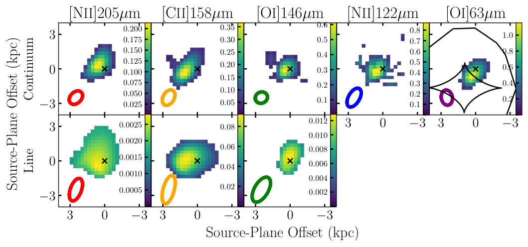
It is simpler to compare the different line and continuum reconstructions if they have comparable resolutions. Therefore, we tapered the visibilities in each data set to before performing the reconstructions. The resolutions are shown as colored ellipses in the lower left corner of the continuum and Moment 0 maps in Figure 4. The effective resolution is , which is gives us resolution. The models, residuals, and error maps are shown in Figure 14 in Appendix A.
III.2 Lens Modeling Results
Figure 4 shows the reconstructed continuum maps and the Moment 0 (integrated flux)maps of the line reconstructions. The continuum maps mostly show similar morphologies, but with different fluxes. As expected, the 63 continuum emission is the brightest and the 205 emission is the weakest. We see differing morphologies in the line emission. The [CII]158 and [NII]205 lines show their brighest emission offset from the [OI]146 emission. Because the Earth’s atmosphere limits access to these lines except at the highest redshifts, the sources with spatially resolved maps of FIR fine structure lines are mostly very nearby galaxies. Parkin et al. 2013 and Herrera-Camus et al. 2018 found in M51 and NGC1068, respectively, that the [CII]158 and [NII] lines had similar morphologies. A similar offset between [OI]146 and [CII]158 emission was seen by Herrera-Camus et al. 2018 in NGC1068. In their maps, the brightest [OI]146 emission was associated with the central AGN in NGC1068, while the [CII]158 emission was associated with the peak in CO emission. Parkin et al. 2013 also found that the [OI]63 and [OI]146 emission peaked in the center of M51, most likely associated with the central AGN, offset from where [CII]158 and [NII]122 emission was strongest. In the SMC, [OI]63 emission was associated with H emission and therefore recent massive star formation (Jameson et al. 2018). As seen in these other systems, the [OI]146 and [OI]63 emission has been associated with regions where one would expect dust heating, whether the dust is being heated by star formation or a central AGN. For SPT0346-52, the [OI]146 emission is concentrated closer to where the dust continuum is strongest. As any potential AGN contribution to the IR emission in SPT0346-52 is negligible (Ma et al. 2016), the [OI]146 emission appears to coincide with the most intense star formation.
Litke et al. 2019 determined that the intense star-formation in SPT0346-52 was driven by a major merger of two components. These components are centered at -310 and +160 km/s and have similar widths ( km/s). The center of these two components lie near -75 km/s. The merger status was determined using position-velocity diagrams of the [CII]158 emission, which is the highest signal-to-noise line of those explored here. Litke et al. 2019 used higher resolution reconstructions than are shown in this work, where we decrease the resolution of the [CII]158 reconstruction to match that of the lowest resolution lines. More recently, Jones et al. 2019 claimed SPT0346-52 is better described as a disk galaxy with a molecular outflow, based on visual inspection of the image-plane structure. However, the candidate H2O outflow Jones et al. 2019 detected is kinematically similar to the blue-shifted component found by Litke et al. 2019. The mass loading factor of the possible outflow in SPT0346-52 is well below unity, unlike other outflows with mass loading factors near or greater than unity. Spilker et al. 2020 do not see broad wings in [CII]158 that would be indicative of outflows in any DSFGs with confirmed molecular outflows traced by blue-shifted OH absorption. Thus, SPT0346-52 is unlikely to host outflow activity. The disk structure described by Jones et al. 2019 may also have resulted from a recent major merger (Hopkins et al. 2009, e.g.,).
IV CLOUDY Modeling
In order to understand the physical conditions that explain our observations, we turn to the photoionization code Cloudy (Ferland et al. 2017, version 17.01;). Cloudy simulates the microphysics within a cloud of gas and dust that is heated by a central source. It predicts the physical conditions throughout the cloud, including temperatures, densities, and metallicities, while also computing a predicted observed spectrum.
IV.1 CLOUDY Parameters
We model our system as an open, or slab-like geometry. We adopt an inner radius (the distance between the central heating source and the inner face of the cloud) of 100 pc. This distance is chosen to be smaller than the size of an individual pixel.
We use the ISM gas-phase elemental abundances and grain size distributions included with Cloudy, which represents the average warm and cold phase abundances of the ISM in the Milky Way (Cowie & Songaila 1986; Savage & Sembach 1996). We also include polycyclic aromatic hydrocarbons (PAHs) in the simulation. Small grains such as PAHs are an important contributor of grain heating mechanisms and FUV radiative transfer effects (Hollenbach & Tielens 1999). For the equation of state of the ISM, we assume constant pressure. The components balanced to achieve constant pressure gas are
| (2) |
where is thermal gas pressure, is the turbulent pressure, is radiation pressure due to trapped emission lines, and is pressure from the attenuation of the incident radiation field. In order to simplify the model, we do not include a magnetic field component. Following Cormier et al. 2019, we assume a constant microturbulent velocity of 1.5 . This is consistent with the microturbulent velocities of individual PDRs (Kaufman et al. 1999; Tielens & Hollenbach 1985).
The gas cloud is heated by a single-burst stellar population. The starburst spectral energy distribution (SED) was compiled by Byler et al. 2017 for use in Cloudy using the Flexible Stellar Population Synthesis code (Conroy et al. 2009; Conroy & Gunn 2010). We use the ionizing spectrum from Byler et al. 2017 produced by the MESA Isochrones and Stellar Tracks (Choi et al. 2016; Dotter 2016, MIST;). The MIST stellar evolution tracks differ from other models in that they include stellar rotation, which results in harder ionizing spectra and higher luminosities (Byler et al. 2017). Byler et al. 2017 compared nebular emission ionized by MIST models to Padova (Bertelli et al. 1994; Girardi et al. 2000; Marigo et al. 2008, for low-mass stars;) and Geneva (Schaller et al. 1992; Meynet & Maeder 2000, for high-mass stars;) evolutionary tracks (Levesque et al. 2010), and found that the MIST models can match observed line ratios better as the starburst ages past a few Myr. We fix the stellar metallicity to and the age to the stellar age calculated by Ma et al. 2015 using SED fitting, Myr. Allowing the stellar metallicity to scale with the gas metallicity did not change our results. The input starburst SED sets the shape of of the ionizing spectrum in cloudy. The intensity of the ionizing radiation is determined by the ionization parameter, described below.
We also include the cosmic microwave background (CMB) at and cosmic rays to contribute to the gas heating. The CMB spectrum was then subtracted from the modeled continuum SED before comparing to the observations, which are measurements of excess above the CMB spectrum.
We create a grid of models varying the ionization parameter (), Hydrogen density () at the face of the cloud, gas metallicity (), and the age of the starburst. The ionization parameter is defined as the ratio of hydrogen-ionizing photons to the total hydrogen density, or more specifically
| (3) |
where is distance between center of starburst and inner surface of cloud (100 pc), is the total hydrogen density, is the number of hydrogen-ionizing photons, and is the speed of light. We vary from -4.5 to -0.5 in steps of 0.25. The total hydrogen density includes molecular, atomic, and ionized hydrogen components. is defined at the inner face of the cloud for the grid values in steps of 0.25. We vary the gas metallicity from in steps of 0.25. We stop the cloudy simulation at visual extiction , following Abel et al. 2009.
To find the best-fit model, we compare the cloudy outputs to a combination of continuum ratios ( 63/122, 63/146, 63/158, 63/205), line ratios ([CII]158/[NII]205, [CII]158/[OI]146), and a line-to-continuum ratio ([OI]146/146) to constrain the relative contributions of gas and dust. The best-fit model is chosen to be the model with the lowest reduced chi-squared value, . Continuum values are in mJy and line values are in . [OI]146/146 has units /mJy. The factor of is used so the line-to-continuum ratio is the same order of magnitude as the continuum ratios and line ratios. Table 6 in the Appendix lists the values used to compare to the cloudy models. We consider both spatially-resolved and galaxy-integrated emission models.
We tested whether the inclusion of the continuum ratios affected our results. When the continuum ratios were not included, the line ratios were still well-fit, but the continuum ratios from cloudy did not match our observations. The ionization parameter was the variable most sensitive to the inclusion of the continuum ratios. This is consistent with previous cloudy modeling, where Abel et al. 2009 found the 60/100 continuum ratio was strongly dependent on the ionization parameter.
IV.2 Cloudy Modeling Results
Figure 5 shows the observed continuum and line ratios with their associated errors, as well as the ratios calculated for the best-fit cloudy model for SPT0346-52. Table 3 lists the best-fit starburst age, , , and values, as well as , for the best-fit models for the global fits shown in Figure 5. Overall, the best-fit models agree with the observed global line and continuum ratios in SPT0346-52.
| Parameter | Value |
|---|---|
| 6.6 |
It is a crude approximation to model an entire galaxy as a single PDR. Indeed, Katz et al. 2019 found in their simulations of emission lines in high-z galaxies that there can be very large ranges in metallicty and ionization parameter across a single galaxy. In the case of SPT0346-52, we have spatially-resolved information about the line and continuum emission and can explore the distribution of properties across the galaxy by fitting our models on a pixel-by-pixel basis. We use the same technique as was used for the galaxy-integrated fits for each pixel. Figure 6 shows the range of values observed and in the best-fit models, as well as the mean values, for each set of continuum and line ratios, while Figure 7 shows the best-fit , , and values in each pixel. For maps of the observed continuum and line ratios, as well as the best-fit model ratios, see Figure 15 in the Appendix.

As with the fits to the global line and continuum ratios, the range of ratios in the pixellated best-fit models mostly agree with the range of ratios observed. The modeled [CII]158/[NII]205 ratios have higher maximum values than the observed ratios, though their average values are more similar. We also see a higher average [CII]158/[OI]146 model ratio than observed, as we did with the galaxy-integrated fit. This may result from the cloudy model not probing far enough from the ionizing source to fully recover line emission from the neutral gas component of the ISM.
The best-fit ionization parameters are around and is relatively uniform. These values are comparable to those found for the DSFG SPT0418-47 (De Breuck et al. 2019, using [NII]205, [CII]158, [OI]146, [NII]122, and [OIII]88;). A popular technique is to report the intensity of the FUV, , relative to the interstellar radiation field, , instead of the ionization parameter. To compare our values to models using , we turn to Figure 1 of Abel et al. 2009; for a starburst SED, and corresponds to . Rybak et al. 2019 and Rybak et al. 2020 found for DSFGs and the DSFG G09.83808, respectively, while Novak et al. 2019 found for the quasar host galaxy J1342+0928. SPT0346-52 has a lower ionization parameter and FUV field strength compared to other high-z DSFGs.
We find densities around throughout this system. This is lower than the inferred densities of the DSFGs SPT0418-47 at (De Breuck et al. 2019, ;) and G09.83808 at (Rybak et al. 2020, ;).
From the cloudy modeling, SPT0346-52 appears to have a supersolar metallicity (). This is higher than other high-z sources that have been found to have metallicities near solar ( for quasar-host galaxy J1342+0928 at and for DSFG SPT0418-47) using [OIII]88/[NII]122 (Novak et al. 2019; De Breuck et al. 2019). However, the [OIII]88/[NII]122 metallicity diagnostic is highly dependent on the ionization parameter (Pereira-Santaella et al. 2017). Using the mass-metallicity relation of elliptical galaxies, Tan et al. 2014 found the metallicity of DSFGs in the protocluster GN20 () to be . The gas to dust ratio, , has been observed to be approximately inversely proportional to the metallicity in galaxies (Magdis et al. 2012; Leroy et al. 2011, e.g.,). Leroy et al. 2011 determined the relation between the gas to dust ratio, and metallicity to be . Using the gas and dust masses from Aravena et al. 2016, in SPT0346-52, giving us , consistent with the cloudy value.
V Discussion
In this section, we explore various diagnostics of the different phases of the ISM in SPT0346-52. We begin with dust emission, then move on to line deficits and the electron density. We then explore the prevalence of ionized versus neutral gas and the non-detection of [OI]63. Finally, we look into several gas mass estimates for different phases of the ISM. For reference, Table 4 lists the transitions explored and their excitation properties. While SPT0346-52 has negligible AGN contribution to its , it is possible there is a highly dust-obscured AGN that prevents X-ray emission from being observed (Ma et al. 2016). DSFGs can contain AGN; for example, Wang et al. 2013 found of DSFGs in the ALESS (ALMA LABOCA E-CDF-S Submm Survey) sample contain AGN. SPT0346-52 may also evolve to contain an AGN (Toft et al. 2014, e.g.,). We therefore consider both DSFGs and quasar-host galaxies for comparison.
| Line | Transitiona | (eV) | (K)b | ()b | ()a | A | ||
|---|---|---|---|---|---|---|---|---|
| [NII]205 | 3P1-3P0 | 1461 | 14.53 | 70 | 3 | |||
| [CII]158 | 2P3/2-2P1/2 | 1901 | 11.26 | 91 | 4 | |||
| [OI]146 | 3P0-3P1 | 2060 | - | 327 | - | 1 | ||
| [NII]122 | 3P2-3P1 | 2459 | 14.53 | 188 | 5 | |||
| [OI]63 | 3P1-3P2 | 4745 | - | 228 | - | 3 |
Note. — The first two columns list the targeted lines and the fine structure transition that emits that line. is the emitted frequency of the line. is the ionization energy needed to remove an electron. is the excitation temperature needed to populate the transition level. is the critical density for collisions with hydrogen at . is the critical density for collisions with electrons at . A is the Einstein A coefficient. is the statistical weight of the upper level.
V.1 Dust Temperatures
We characterize the FIR continuum and dust temperatures throughout the source-plane using a modified blackbody function. We use the form from Spilker et al. 2016,
| (4) |
is the Planck function at rest-frame frequency and temperature . The blackbody is modified by the dust optical depth, , which at long wavelengths can be parameterized by . In this parameterization, the optical depth reaches unity at wavelength , which together with determines the peak wavelength and the width of the peak of the dust emission. The slope of the Rayleigh-Jeans tail of dust emission is . Typically, and in the rest-frame (Casey et al. 2014, e.g.,).
This modified blackbody is used to fit for the dust temperature in each pixel of the source-plane reconstruction, as well as the global dust temperature. Five continuum bands (63, 122, 146, 158, and 205) are used to fit the SEDs. Because of the limited number of photometric points available for these fits, we follow Greve et al. 2012 by fixing and . There are two free parameters in each SED fit, the dust temperature, , and the normalization.

The top panel of Figure 8 shows the global SED fit (black line) to the continuum (colored stars). For SPT0346-52, we calculate . The grey lines show the best-fit SEDs for the individual pixels. The best-fit dust temperatures are shown in the bottom center panel of Figure 8, while the right panel shows the error on the best-fit dust temperatures in each pixel. The left panel shows the FIR surface density (). is calculated here as the integral of the best-fit modified blackbody SED from (Helou et al. 1988). To get , we divide by the source-plane pixel area in . Dust temperature values in individual pixels have a mean .
Dust temperatures can vary significantly depending on the fitting form used (Hayward et al. 2012, e.g., ). Casey et al. 2014 show how, for a given , the dust temperature can vary by up to 40 K depending on what assumptions are made about the opacity, as well as the value of used. The dust temperatures we calculate are lower than that calculated by Reuter et al. 2020 using Equation 4 ( for SPT0346-52). However, this temperature difference is a result of the fitting procedures used in this work and by Reuter et al. 2020. Reuter et al. 2020 use the relation between and found by Spilker et al. 2016. Using this relation tends to increase the fitted dust temperature by (Reuter et al. 2020). Jones et al. 2020 also calculated for SPT0346-52, using a modified blackbody distribution with effects from the CMB. The small uncertainty is largely due to the unrealistically small photometric errors claimed for the data used in the fit, many of which are well below 1%. Using the model from Jones et al. 2020 and the data from this paper, we calculate . Apostolovski et al. 2019 calculated for SPT0346-52 by using a radiative transfer model. The significant difference from the results of the continuum SED fits presented above undoubtedly results from the difference in methodology and the impact of including CO excitation as a constraint on the dust temperature.
V.2 Line Deficits
A commonly observed phenomenon is the so-called “[CII] deficit”, where falls as increases (Luhman et al. 1998; Sargsyan et al. 2012; Farrah et al. 2013; Oteo et al. 2016; Spilker et al. 2016; Gullberg et al. 2018, e.g.,). Here, we explore possible deficits in other FIR lines that trace different components of the ISM. Figure 9 shows the line-to-FIR luminosity ratios versus for the five lines in this work. In SPT0346-52, we see deficits, i.e., apparent trends with , in all five lines. Additionally, we see spatially-resolved deficits (apparent trends with in individual pixels) in all three detected lines.
Graciá-Carpio et al. 2011 found deficits in [CII]158, [NII]122, [OI]146 and [OI]63, concluding that line deficits occurred in both ionized and neutral gas in galaxies with a variety of redshifts and optical classifications. They explained the deficits as resulting from an increase in the ionization parameter at / as highly compressed, more efficient star formation leads to enhanced ionization parameters. Zhao et al. 2016 found that there was only a [NII]205 deficit in LIRGs that had warm () colors. SPT0346-52 falls into this warm-color regime and does indeed exhibit an [NII]205 deficit. On the other hand, several individual sources, ranging from main sequence galaxies to quasar host galaxies, did not show lower [OI]146/ (Li et al. 2020) and [OI]63/ ratios (Wagg et al. 2020; Coppin et al. 2012; Sturm et al. 2010). In the spatially resolved SHINING galaxies, a sample of nearby galaxies that includes star-forming galaxies, AGN host galaxies, and LIRGs, Herrera-Camus et al. 2018 found the trend of decreasing line/ strongest for singly ionized lines like [NII]122 and [CII]158 and weakest for neutral [OI]146 and [OI]63.
V.3 [CII]158/[NII]205
Carbon has an ionization potential of 11.26 eV, which is slightly lower than that of hydrogen. This makes interpretation of [CII]158 emission difficult because it can originate from both ionized and neutral regions of the ISM. By comparing the [CII]158 to the [NII]205 emission, which arises only in ionized regions, we can infer how the [CII]158 emission is divided between neutral and ionized gas.
We can calculate the fraction of [CII]158 emission originating from neutral gas by comparing the observed [CII]158/[NII]205 ratio to the expected ratio. From Abdullah et al. 2017,
| (5) |
where is the expected line intensity ratio, is the expected line intensity of the transition, is the upper-level population, is the energy of the transition, and is the Einstein coefficient for that transition. This relation assumes the ionic abundance ratio, [CII]158/[NII]205 is equal to the elemental abundance ratio, . also depends on . As seen in Table 4, [CII]158 and [NII]205 have similar critical electron densities ( and ). Therefore, if we compute the expected [CII]158/[NII]205 ratio, there is little density dependence.
Croxall et al. 2017 calculated using collision rates from Tayal 2008 ([CII]158) and Tayal 2011 ([NII]205) and assuming Galactic gas-phase abundances for both elements, while Díaz-Santos et al. 2017 used , based on photoionization models by Oberst et al. 2006. We adopt an intermediate value of . With this expected [CII]158/[NII]205 ratio, we can calculate the fraction of [CII]158 from neutral gas, , using
| (6) |
For SPT0346-52, we calculate . Nearby galaxies ranging from low-metallicity dwarf galaxies (Cormier et al. 2019) to star-forming galaxies (Sutter et al. 2019; Herrera-Camus et al. 2018) and (U)LIRGs (Díaz-Santos et al. 2017) have . As shown in Figure 10, SPT0346-52 has a more comparable to what has been observed in other high-z sources and DSFGs (Li et al. 2020; De Breuck et al. 2019; Pavesi et al. 2018; Zhang et al. 2018, , e.g.,). This fraction has been observed to be higher in active star-forming regions (Herrera-Camus et al. 2018) and LIRGs with warmer colors (Díaz-Santos et al. 2017) like SPT0346-52.

V.4 [CII]158/[OI]146
[CII]158 originates from both ionized and neutral gas, while [OI]146 emission arises from only neutral regions. Therefore, more [OI]146 emission would indicate the presence of more dense, neutral gas. The ratio of these lines has therefore been used in the literature as an indicator of the prevalence of dense gas (De Breuck et al. 2019; Li et al. 2020).

Figure 11 plots as a function of for SPT0346-52, both integrated and spatially resolved, and values from the literature. SPT0346-52 has similar [CII]158/[OI]146 ratio compared to galaxies in the SHINING sample (Herrera-Camus et al. 2018). It is higher than SPT0418-47, a lensed DSFG. De Breuck et al. 2019 determined that SPT0418-47 had an [CII]158/[OI]146 ratio lower than local galaxies, leading them to conclude that the ISM in SPT0418-47 is dominated by dense gas. Li et al. 2020 also found [CII]158/[OI]146 in their quasar was comparable to the lowest values in ULIRGs, implying that SDSS J2310+1855 has warmer and denser gas compared to local galaxies. The higher [CII]158/[OI]146 ratio in SPT0346-52, implying a smaller dense gas component, is consistent with the lower hydrogen gas densities found using cloudy in Section IV.2.
V.5 Non-Detection of [NII]122
[NII]122 is expected to be brighter than [NII]205. However, due to atmospheric O2 at 368.5GHz, just km/s from the expected center of the [NII]122 emisssion, [NII]122 is not detected in SPT0346-52. However, we can use the upper limit obtained in Section II to place constraints on the ISM conditions.
Nitrogen ions are only expected to be found in ionized regions of the ISM. In this regime, the [NII]122 and [NII]205 fine structure lines would be excited mostly through collisions with electrons (Goldsmith et al. 2015). Therefore, the relative intensity of [NII]122 compared to [NII]205 will depend on the electron density of the ISM and can be used to calculate this density.
We calculate the theoretical relation between the [NII]122/[NII]205 flux ratio and the electron density, , following Goldsmith et al. 2015 and using the collision rate coefficients from Tayal 2011. This relation is shown as the grey line in Figure 12. The left panel also shows the upper-limit to the ratios and corresponding values for SPT0346-52.
In SPT0346-52, we find . The densities observed in SPT0346-52 are lower than the densities calculated in other, comparable systems using the [NII]122/[NII]205 ratio. For example, Díaz-Santos et al. 2017 found a median for local LIRGs, with densities ranging from (black dashed and dotted lines in Figure 12), comparable to those found by Zhao et al. 2016, while De Breuck et al. 2019 calculated for the lensed DSFG SPT0418-47. The non-detection of [NII]122 indicates low densities in the ionized phase of the ISM.
V.6 Non-Detection of [OI]63
[CII]158 and [OI]63 are both major coolants of the ISM. As one transitions to high-density (), high-temperature (), high-radiation () regimes, [OI]63 becomes the dominant coolant over [CII]158 (Tielens & Hollenbach 1985; Hollenbach et al. 1991). One would expect to find bright [OI]63 emission comparable to or greater than the [CII]158 emission in FIR-bright systems like starbursts, where the ISM is heated by strong FUV radiation and warmer, denser gas is expected (Tielens & Hollenbach 1985). In the first detection of [OI]63, Rybak et al. 2020 found [OI]63 was times brighter than [CII]158 in the DSFG, G09.83808. Given the intense star formation in SPT0346, we could reasonably expect that [OI]63 might be significantly more luminous than [CII]158. However, we are unable to detect this line in our observations, finding a luminosity ratio of . Our inability to place a tighter detection limit reflects the impact of atmospheric O2 absorption centered at 715.4 GHz, just km/s from the redshifted [OI]63 line center.
The [OI]63 emission may be intrinsically weak. Spinoglio & Malkan 1992 also found lower [OI]63 intensities with their cloudy modeling of starburst regions. In addition, Abel et al. 2009 found that low values of the ionization parameter, , were associated with lower [OI]63/[CII]158 ratio in their cloudy models of ULIRGs. For SPT0346-52, [OI]63/[CII]158, which is lower than [OI]63/[CII]158 in the DSFG G09.83808 (Rybak et al. 2020). Rybak et al. 2020 found (corresponding to ), which is higher than the values found in SPT0346-52. Our cloudy modeling of SPT0346-52 indicates lower ionization parameters, consistent with the lower [OI]63/[CII]158 ratio.
Often [OI]63 is optically thick (Liseau et al. 2006; Kaufman et al. 1999; Tielens & Hollenbach 1985). It is also easily self-absorbed; small amounts of cold foreground gas can absorb [OI]63 while leaving [OI]146 unaffected (Liseau et al. 2006). This effect has been measured to reduce the [OI]63 emission by factors of (Kramer et al. 2020) up to (Liseau et al. 2006). If [OI]63/[OI]146 , [OI]63 is likely self-absorbed (Díaz-Santos et al. 2017; Cormier et al. 2015; Tielens & Hollenbach 1985). Taking the upper limit and correcting for the lensing magnification, [OI]63/[OI]146 in SPT0346-52. The [OI]63/[OI]146 intensity ratio may be , so [OI]63 may be self-absorbed.
The [OI]63/[CII]158 ratio may also be influenced by the presence of an AGN. With its high critical density (Table 4), [OI]63 is produced primarily in dense, neutral gas. In models of PDRs and X-ray dominated regions (XDRs), the [OI]63/[CII]158 ratio is higher in XDRs (which are expected near AGN) than in PDRs (Maloney et al. 1996; Meijerink et al. 2007). Ma et al. 2016 found no evidence of AGN activity in this source, so we do not expect an AGN-based enhancement of [OI]63 emission.
V.7 Gas Mass Estimates
In this section, we estimate the ionized, neutral, and molecular gas masses using the various fine-structure lines observed in SPT0346-52. For ease of comparison, and because of the higher metallicity expected by gas to dust mass ratio in SPT0346-52, the ionic abundances are assumed to be the same as the global abundances in HII regions from Savage & Sembach 1996 (i.e., ([CII]) = C/H, ([NII]) = N/H, and ([OI]) = O/H). Table 5 lists a summary of the different masses calculated using the various methods described below. Figure 13 shows the various masses calculated for SPT0346-52 and several other high-redshift sources, normalized by the molecular gas mass calculated using CO.
| Mass Type | Line or Reference | SPT0346-52 |
|---|---|---|
| ( ) | ||
| Dust | 1 | |
| 2 | ||
| Molecular | 2 | |
| 3 | ||
| Stellar | 4 | |
| Molecular | [CII]158 | |
| PDR | [CII]158 | |
| Neutral | [CII]158 | |
| [OI]146 | ||
| Ionized | [NII]205 |
V.7.1 Molecular Gas Mass from
In their study of main sequence galaxies, Zanella et al. 2018 found that the [CII]158 luminosity and the molecular gas mass of a galaxy were correlated. /, with a standard deviation of 0.3 dex, is mostly independent of depletion time, metallicity, and redshift.
Using our observed [CII]158 luminosity, we find a molecular gas mass of . This is between the molecular gas mass calculated by Aravena et al. 2016 using CO () and the molecular gas mass calculated by Apostolovski et al. 2019 using radiative transfer modeling ().
Zanella et al. 2018 calibrated using main sequence galaxies at . However, for DSFGs and quasar host galaxies, this method tends to result in higher molecular gas masses than those obtained using CO, as shown by the green points in Figure 13. The molecular masses calculated using are also higher than the neutral gas masses calculated using the method in Section V.7.3 in both this work and previous studies (Decarli et al. 2019; Novak et al. 2019).
V.7.2 Neutral Gas Mass from [CII]158 PDR Modeling
Hailey-Dunsheath et al. 2010 calculate the atomic mass associated with PDRs in the hyperluminous starburst galaxy MIPS J1428 using the [CII]158 luminosity and PDR models from Kaufman et al. 1999. Assuming the [CII]158 emission is optically thin and that a single temperature characterizes the [CII]158-emitting region, the PDR mass is given by
| (7) |
Following Hailey-Dunsheath et al. 2010, we assume the gas temperature is the surface temperature of their modeled PDR, , , (Launay & Roueff 1977), and (Savage & Sembach 1996). We use our calculated value of . We calculate a PDR mass of for SPT0346-52. This is of the total gas mass from Aravena et al. 2016.
The PDR mass fraction calculated for SPT0346-52 is much lower than that found by Hailey-Dunsheath et al. 2010 for MIPS J1428 (). We also find a similarly lower PDR mass compared to the molecular gas mass in SPT0346-52 than in HFLS3 (Riechers 2013, ;), and SDP.11 (Lamarche et al. 2018, ;). This method assumes a gas density , higher than the density found using cloudy (Section IV.2). If we instead use , we calculate an atomic PDR mass fraction of , which is more comparable to other high-z sources. This discrepancy could explain the difference in atomic PDR masses between SPT0346-52 and other high-z sources. Masses calculated with this method are shown as silver points in Figure 13.
V.7.3 Neutral Gas Masses from [CII]158 and [OI]146
We next estimate the neutral gas mass in SPT0346-52 using [CII]158 and [OI]146. Based on the work by Weiß et al. 2005 and Li et al. 2020, the mass associated with a single transition can be calculated using
| (8) |
where is the mass of atom , is the emission frequency, is the Einstein coefficient, is the partition function, is the statistical weight of the upper level, is the Boltzmann constant, is the Planck constant, is the excitation temperature needed to populate the transition level from Table 4, is the excitation temperature of the gas, and is line luminosity in . The Einstein A coefficients, upper level statistical weights, and transition temperatures can be found in Table 4.
We adopt an excitation temperature of . Based on PDR modeling by Meijerink et al. 2007, is the temperature of a PDR cloud near the outer regions where [CII]158 is primarily emitted. The cloud will cool off to in the inner parts of the cloud as carbon transitions from [CII] to neutral C to CO. We also use this temperature for the [OI]146-based mass calculation. This method assumes the [CII]158 and [OI]146 emission is optically thin.
For [CII]158 , Equation 8 becomes
| (9) |
where and is multiplied by so only the neutral gas contribution to the [CII]158 emission is included. Decarli et al. 2019 argue that the mass calculated using [CII]158 is a lower limit as it does not include non-ionized carbon or effects from lower metallicty gas, suppressed [CII]158 emission from collisional de-excitation, and optical depth effects.
For [OI]146, we can calculate the oxygen mass using
| (10) |
In this case, .
To get the neutral gas mass, we divide by the or abundance. Using the abundance from Savage & Sembach 1996 ( and ), we find neutral gas masses of and . The [CII]158 and [OI]146 neutral gas masses are approximately one-quarter the total gas mass calculated by Aravena et al. 2016. In general, the neutral gas masses calculated using [CII]158, [OI]146, and [CI]369 in both SPT0346-52 and in dusty star-forming galaxies and quasar host galaxies in the literature are within a factor of of the molecular gas mass (blue points in Figure 13).
The mass calculated using [CII]158 is higher than the mass calculated using [CII]158 and PDR modeling in Section V.7.2. While two different temperatures were used (230 K vs 100 K), this difference only changes the calculated masses by and does not fully account for the large discrepancy in the mass estimates. The mass estimate in Section V.7.2 is based on the PDR model of a cloud illuminated on one side from Kaufman et al. 1999. As discussed in Section IV, this is a simple model compared to the complexity of a galaxy. On the other hand, the method used in this section assumes optically thin emission and that the lines are in local thermodynamic equilibrium. These assumptions may not be valid for all of the [CII]158 emission in SPT0346-52 and could also account for the discrepancy between the [CII]158 neutral gas mass estimates. In addition, as discussed in Section V.7.2, the discrepancy also arises from the density of the gas in the PDR model. Using from our cloudy modeling instead of from Hailey-Dunsheath et al. 2010 results in consistent PDR masses using the different methods.
V.7.4 Ionized Gas Mass
Following the method Ferkinhoff et al. 2010 used for [OIII]88 and Ferkinhoff et al. 2011 adapted for [NII]122, we can calculate the minimum ionized gas mass required to produce the observed [NII]205 emission. This method assumes all the nitrogen in the HII regions is singly ionized, and that the gas is in the high-temperature limit as would be expected in active star-forming regions. With these assumptions, we can calculate the minimum ionized gas mass using
| (11) |
Here, is the Planck constant and is the mass of the Hydrogen atom. In the high temperature limit, the partition function of [NII]205 is . , , and can all be found in Table 4. Using the nitrogen abundance from Savage & Sembach 1996, , we find a minimum ionized gas mass of .
Ferkinhoff et al. 2011 found that is correlated with , where more intensely star-forming galaxies have higher fractions of ionized gas. The minimum ionized gas mass in SPT0346-52 is of the total molecular gas mass from Aravena et al. 2016. These values are lower than the ionized gas mass fractions determined for the Cloverleaf (Ferkinhoff et al. 2011, ) and J1342+0928 (Novak et al. 2019, ). As mentioned above, this method assumes the gas is in the high-temperature limit. This is likely not the case for SPT0346-52. At lower temperatures, more mass will be required to produce the observed [NII]205 emission. The ionized gas masses calculated here are therefore lower limits to the total ionized gas mass.
As shown in Figure 13, the molecular phase is the most significant mass component in SPT0346-52. There is more molecular gas than neutral gas and more molecular gas than ionized gas. This is in contrast to galaxies in the nearby universe; for example, the Milky Way has a molecular gas mass ( ) very close to its ionized gas mass ( ), and more than twice as much atomic gas compared to molecular gas (Ferrière 2001). The large molecular gas reservoir in SPT0346-52 fuels the large star formation rate observed in this system.
VI Summary and Conclusions
In this work we present ALMA Bands 6, 7, and 9 observations of [NII]205, [CII]158, [OI]146, and undetected [NII]122 and [OI]63, as well as the underlying continuum at all five wavelengths, in the lensed dusty star-forming galaxy SPT0346-52. We reconstruct the lensed continuum and line data using the pixelated, interferometric lens modeling code ripples in order to study the source-plane structure of SPT0346-52. We analyze both the galaxy-integrated properties and the spatially resolved properties of SPT0346-52.
We use the photoionization code cloudy to model the physical conditions of the ISM in SPT0346-52. It has lower ionization parameter () and hydrogen density () than other high-z DSFGs. Based on cloudy modeling, we find supersolar metallicity (), similar than would be expected from the gas to dust ratio in SPT0346-52.
We calculate the dust temperatures throughout SPT0346 and compare the global dust temperature and the wavelength where the SED peaks to other models. We look at line deficits and find deficits in all five lines and spatially-resolved deficits in all three detected lines, [NII]205, [CII]158, and [OI]145. We use the limit on the [NII]122/[NII]205 ratio to find in SPT0346-52, which is lower than what is observed in ULIRGs and other DSFGs. Using [CII]158/[NII]205, we determine of the [CII]158 emission originates from neutral gas, comparable to other high-z sources and ULIRGs. Using the [CII]158/[OI]146 ratio, we see that SPT0346-52 has similar dense gas in PDRs to local galaxies.
Finally, we calculate ionized, neutral, and molecular gas masses using a variety of methods. The molecular gas mass is the ionized gas mass and the neutral atomic gas mass. The molecular ISM dominates the mass budget of SPT0346-52, fueling the intense star-formation in this system.
References
- Abdullah et al. (2017) Abdullah, A., Brandl, B. R., Groves, B., et al. 2017, ApJ, 842, 4
- Abel et al. (2009) Abel, N. P., Dudley, C., Fischer, J., Satyapal, S., & van Hoof, P. A. M. 2009, ApJ, 701, 1147
- Apostolovski et al. (2019) Apostolovski, Y., Aravena, M., Anguita, T., et al. 2019, A&A, 628, A23
- Aravena et al. (2016) Aravena, M., Spilker, J. S., Bethermin, M., et al. 2016, MNRAS, 457, 4406
- Bañados et al. (2019) Bañados, E., Novak, M., Neeleman, M., et al. 2019, ApJ, 881, L23
- Bertelli et al. (1994) Bertelli, G., Bressan, A., Chiosi, C., Fagotto, F., & Nasi, E. 1994, A&AS, 106, 275
- Béthermin et al. (2020) Béthermin, M., Fudamoto, Y., Ginolfi, M., et al. 2020, A&A, 643, A2
- Byler et al. (2017) Byler, N., Dalcanton, J. J., Conroy, C., & Johnson, B. D. 2017, ApJ, 840, 44
- Carlstrom et al. (2011) Carlstrom, J. E., Ade, P. A. R., Aird, K. A., et al. 2011, PASP, 123, 568
- Casey et al. (2014) Casey, C. M., Narayanan, D., & Cooray, A. 2014, Phys. Rep., 541, 45
- Choi et al. (2016) Choi, J., Dotter, A., Conroy, C., et al. 2016, ApJ, 823, 102
- Conroy & Gunn (2010) Conroy, C., & Gunn, J. E. 2010, ApJ, 712, 833
- Conroy et al. (2009) Conroy, C., Gunn, J. E., & White, M. 2009, ApJ, 699, 486
- Cooray et al. (2014) Cooray, A., Calanog, J., Wardlow, J. L., et al. 2014, ApJ, 790, 40
- Coppin et al. (2012) Coppin, K. E. K., Danielson, A. L. R., Geach, J. E., et al. 2012, MNRAS, 427, 520
- Cormier et al. (2015) Cormier, D., Madden, S. C., Lebouteiller, V., et al. 2015, A&A, 578, A53
- Cormier et al. (2019) Cormier, D., Abel, N. P., Hony, S., et al. 2019, A&A, 626, A23
- Cowie & Songaila (1986) Cowie, L. L., & Songaila, A. 1986, ARA&A, 24, 499
- Croxall et al. (2017) Croxall, K. V., Smith, J. D., Pellegrini, E., et al. 2017, ApJ, 845, 96
- Cunningham et al. (2020) Cunningham, D. J. M., Chapman, S. C., Aravena, M., et al. 2020, MNRAS, 494, 4090
- De Breuck et al. (2019) De Breuck, C., Weiß, A., Béthermin, M., et al. 2019, A&A, 631, A167
- Decarli et al. (2014) Decarli, R., Walter, F., Carilli, C., et al. 2014, ApJ, 782, L17
- Decarli et al. (2019) Decarli, R., Dotti, M., Bañados, E., et al. 2019, ApJ, 880, 157
- Díaz-Santos et al. (2017) Díaz-Santos, T., Armus, L., Charmandaris, V., et al. 2017, ApJ, 846, 32
- Dotter (2016) Dotter, A. 2016, ApJS, 222, 8
- Everett et al. (2020) Everett, W. B., Zhang, L., Crawford, T. M., et al. 2020, ApJ, 900, 55
- Farrah et al. (2013) Farrah, D., Lebouteiller, V., Spoon, H. W. W., et al. 2013, ApJ, 776, 38
- Ferkinhoff et al. (2010) Ferkinhoff, C., Hailey-Dunsheath, S., Nikola, T., et al. 2010, ApJ, 714, L147
- Ferkinhoff et al. (2011) Ferkinhoff, C., Brisbin, D., Nikola, T., et al. 2011, ApJ, 740, L29
- Ferland et al. (2017) Ferland, G. J., Chatzikos, M., Guzmán, F., et al. 2017, RMxAA, 53, 385
- Ferrière (2001) Ferrière, K. M. 2001, Reviews of Modern Physics, 73, 1031
- Girardi et al. (2000) Girardi, L., Bressan, A., Bertelli, G., & Chiosi, C. 2000, A&AS, 141, 371
- Goldsmith et al. (2015) Goldsmith, P. F., Yıldız, U. A., Langer, W. D., & Pineda, J. L. 2015, ApJ, 814, 133
- Graciá-Carpio et al. (2011) Graciá-Carpio, J., Sturm, E., Hailey-Dunsheath, S., et al. 2011, ApJ, 728, L7
- Greve et al. (2012) Greve, T. R., Vieira, J. D., Weiß, A., et al. 2012, ApJ, 756, 101
- Gullberg et al. (2015) Gullberg, B., De Breuck, C., Vieira, J. D., et al. 2015, MNRAS, 449, 2883
- Gullberg et al. (2018) Gullberg, B., Swinbank, A. M., Smail, I., et al. 2018, ApJ, 859, 12
- Hailey-Dunsheath et al. (2010) Hailey-Dunsheath, S., Nikola, T., Stacey, G. J., et al. 2010, ApJ, 714, L162
- Hayward et al. (2012) Hayward, C. C., Jonsson, P., Kereš, D., et al. 2012, MNRAS, 424, 951
- Helou et al. (1988) Helou, G., Khan, I. R., Malek, L., & Boehmer, L. 1988, ApJS, 68, 151
- Herrera-Camus et al. (2018) Herrera-Camus, R., Sturm, E., Graciá-Carpio, J., et al. 2018, ApJ, 861, 94
- Hezaveh et al. (2013) Hezaveh, Y. D., Marrone, D. P., Fassnacht, C. D., et al. 2013, ApJ, 767, 132
- Hezaveh et al. (2016) Hezaveh, Y. D., Dalal, N., Marrone, D. P., et al. 2016, ApJ, 823, 37
- Hollenbach et al. (1991) Hollenbach, D. J., Takahashi, T., & Tielens, A. G. G. M. 1991, ApJ, 377, 192
- Hollenbach & Tielens (1999) Hollenbach, D. J., & Tielens, A. G. G. M. 1999, Reviews of Modern Physics, 71, 173
- Hopkins et al. (2009) Hopkins, P. F., Cox, T. J., Younger, J. D., & Hernquist, L. 2009, ApJ, 691, 1168
- Iono et al. (2006) Iono, D., Tamura, Y., Nakanishi, K., et al. 2006, PASJ, 58, 957
- Ivison et al. (2010) Ivison, R. J., Smail, I., Papadopoulos, P. P., et al. 2010, MNRAS, 404, 198
- Jameson et al. (2018) Jameson, K. E., Bolatto, A. D., Wolfire, M., et al. 2018, ApJ, 853, 111
- Jarugula et al. (2021) Jarugula, S., Vieira, J. D., Weiß, A., et al. 2021, arXiv e-prints, arXiv:2108.11319
- Jones et al. (2019) Jones, G. C., Maiolino, R., Caselli, P., & Carniani, S. 2019, A&A, 632, L7
- Jones et al. (2020) —. 2020, MNRAS, 498, 4109
- Katz et al. (2019) Katz, H., Galligan, T. P., Kimm, T., et al. 2019, MNRAS, 487, 5902
- Kaufman et al. (1999) Kaufman, M. J., Wolfire, M. G., Hollenbach, D. J., & Luhman, M. L. 1999, ApJ, 527, 795
- Kramer et al. (2020) Kramer, C., Nikola, T., Anderl, S., et al. 2020, A&A, 639, A61
- Lamarche et al. (2018) Lamarche, C., Verma, A., Vishwas, A., et al. 2018, ApJ, 867, 140
- Launay & Roueff (1977) Launay, J. M., & Roueff, E. 1977, A&A, 56, 289
- Le Fèvre et al. (2020) Le Fèvre, O., Béthermin, M., Faisst, A., et al. 2020, A&A, 643, A1
- Lee et al. (2019) Lee, M. M., Nagao, T., De Breuck, C., et al. 2019, ApJ, 883, L29
- Lee et al. (2021) —. 2021, ApJ, 913, 41
- Leroy et al. (2011) Leroy, A. K., Bolatto, A., Gordon, K., et al. 2011, ApJ, 737, 12
- Levesque et al. (2010) Levesque, E. M., Kewley, L. J., & Larson, K. L. 2010, AJ, 139, 712
- Li et al. (2020) Li, J., Wang, R., Cox, P., et al. 2020, ApJ, 900, 131
- Liseau et al. (2006) Liseau, R., Justtanont, K., & Tielens, A. G. G. M. 2006, A&A, 446, 561
- Litke et al. (2019) Litke, K. C., Marrone, D. P., Spilker, J. S., et al. 2019, ApJ, 870, 80
- Lu et al. (2017) Lu, N., Zhao, Y., Díaz-Santos, T., et al. 2017, ApJS, 230, 1
- Luhman et al. (1998) Luhman, M. L., Satyapal, S., Fischer, J., et al. 1998, ApJ, 504, L11
- Lutz et al. (2016) Lutz, D., Berta, S., Contursi, A., et al. 2016, A&A, 591, A136
- Ma et al. (2015) Ma, J., Gonzalez, A. H., Spilker, J. S., et al. 2015, ApJ, 812, 88
- Ma et al. (2016) Ma, J., Gonzalez, A. H., Vieira, J. D., et al. 2016, ApJ, 832, 114
- Magdis et al. (2012) Magdis, G. E., Daddi, E., Béthermin, M., et al. 2012, ApJ, 760, 6
- Maloney et al. (1996) Maloney, P. R., Hollenbach, D. J., & Tielens, A. G. G. M. 1996, ApJ, 466, 561
- Marigo et al. (2008) Marigo, P., Girardi, L., Bressan, A., et al. 2008, A&A, 482, 883
- Marrone et al. (2018) Marrone, D. P., Spilker, J. S., Hayward, C. C., et al. 2018, Nature, 553, 51
- McMullin et al. (2007) McMullin, J. P., Waters, B., Schiebel, D.and Young, W., & Golap, K. 2007, in ASP Conf. Ser. 376, ed. R. A. Shaw, F. Hill, & D. J. Bell (San Francisco, CA: ASP), 127
- Meijerink et al. (2007) Meijerink, R., Spaans, M., & Israel, F. P. 2007, A&A, 461, 793
- Meynet & Maeder (2000) Meynet, G., & Maeder, A. 2000, A&A, 361, 101
- Novak et al. (2019) Novak, M., Bañados, E., Decarli, R., et al. 2019, ApJ, 881, 63
- Oberst et al. (2006) Oberst, T. E., Parshley, S. C., Stacey, G. J., et al. 2006, ApJ, 652, L125
- Oteo et al. (2016) Oteo, I., Ivison, R. J., Dunne, L., et al. 2016, ApJ, 827, 34
- Parkin et al. (2013) Parkin, T. J., Wilson, C. D., Schirm, M. R. P., et al. 2013, ApJ, 776, 65
- Pavesi et al. (2016) Pavesi, R., Riechers, D. A., Capak, P. L., et al. 2016, ApJ, 832, 151
- Pavesi et al. (2018) Pavesi, R., Riechers, D. A., Sharon, C. E., et al. 2018, ApJ, 861, 43
- Pensabene et al. (2021) Pensabene, A., Decarli, R., Bañados, E., et al. 2021, A&A, 652, A66
- Pereira-Santaella et al. (2017) Pereira-Santaella, M., Rigopoulou, D., Farrah, D., Lebouteiller, V., & Li, J. 2017, MNRAS, 470, 1218
- Petry & CASA Development Team (2012) Petry, D., & CASA Development Team. 2012, in Astronomical Society of the Pacific Conference Series, Vol. 461, Astronomical Data Analysis Software and Systems XXI, ed. P. Ballester, D. Egret, & N. P. F. Lorente, 849
- Planck Collaboration et al. (2016) Planck Collaboration, Ade, P. A. R., Aghanim, N., et al. 2016, A&A, 594, A13
- Reuter et al. (2020) Reuter, C., Vieira, J. D., Spilker, J. S., et al. 2020, ApJ, 902, 78
- Riechers (2013) Riechers, D. A. 2013, ApJ, 765, L31
- Rybak et al. (2020) Rybak, M., Zavala, J. A., Hodge, J. A., Casey, C. M., & Werf, P. v. d. 2020, ApJ, 889, L11
- Rybak et al. (2019) Rybak, M., Calistro Rivera, G., Hodge, J. A., et al. 2019, ApJ, 876, 112
- Sargsyan et al. (2012) Sargsyan, L., Lebouteiller, V., Weedman, D., et al. 2012, ApJ, 755, 171
- Savage & Sembach (1996) Savage, B. D., & Sembach, K. R. 1996, ARA&A, 34, 279
- Schaller et al. (1992) Schaller, G., Schaerer, D., Meynet, G., & Maeder, A. 1992, A&AS, 96, 269
- Shao et al. (2019) Shao, Y., Wang, R., Carilli, C. L., et al. 2019, ApJ, 876, 99
- Spilker et al. (2015) Spilker, J. S., Aravena, M., Marrone, D. P., et al. 2015, ApJ, 811, 124
- Spilker et al. (2016) Spilker, J. S., Marrone, D. P., Aravena, M., et al. 2016, ApJ, 826, 112
- Spilker et al. (2020) Spilker, J. S., Phadke, K. A., Aravena, M., et al. 2020, ApJ, 905, 85
- Spinoglio & Malkan (1992) Spinoglio, L., & Malkan, M. A. 1992, ApJ, 399, 504
- Stacey (2011) Stacey, G. J. 2011, IEEE Transactions on Terahertz Science and Technology, 1, 241
- Sturm et al. (2010) Sturm, E., Verma, A., Graciá-Carpio, J., et al. 2010, A&A, 518, L36
- Sutter et al. (2019) Sutter, J., Dale, D. A., Croxall, K. V., et al. 2019, ApJ, 886, 60
- Suyu et al. (2006) Suyu, S. H., Marshall, P. J., Hobson, M. P., & Blandford, R. D. 2006, MNRAS, 371, 983
- Tan et al. (2014) Tan, Q., Daddi, E., Magdis, G., et al. 2014, A&A, 569, A98
- Tayal (2008) Tayal, S. S. 2008, A&A, 486, 629
- Tayal (2011) —. 2011, ApJS, 195, 12
- Tielens & Hollenbach (1985) Tielens, A. G. G. M., & Hollenbach, D. 1985, ApJ, 291, 722
- Toft et al. (2014) Toft, S., Smolčić, V., Magnelli, B., et al. 2014, ApJ, 782, 68
- Venemans et al. (2017) Venemans, B. P., Walter, F., Decarli, R., et al. 2017, ApJ, 851, L8
- Vieira et al. (2010) Vieira, J. D., Crawford, T. M., Switzer, E. R., et al. 2010, ApJ, 719, 763
- Vieira et al. (2013) Vieira, J. D., Marrone, D. P., Chapman, S. C., et al. 2013, Nature, 495, 344
- Wagg et al. (2020) Wagg, J., Aravena, M., Brisbin, D., et al. 2020, MNRAS, 499, 1788
- Wang et al. (2013) Wang, S. X., Brandt, W. N., Luo, B., et al. 2013, ApJ, 778, 179
- Warren & Dye (2003) Warren, S. J., & Dye, S. 2003, ApJ, 590, 673
- Weiß et al. (2005) Weiß, A., Downes, D., Henkel, C., & Walter, F. 2005, A&A, 429, L25
- Weiß et al. (2007) Weiß, A., Downes, D., Neri, R., et al. 2007, A&A, 467, 955
- Weiß et al. (2003) Weiß, A., Henkel, C., Downes, D., & Walter, F. 2003, A&A, 409, L41
- Weiß et al. (2013) Weiß, A., De Breuck, C., Marrone, D. P., et al. 2013, ApJ, 767, 88
- Wright (2006) Wright, E. L. 2006, PASP, 118, 1711
- Zanella et al. (2018) Zanella, A., Daddi, E., Magdis, G., et al. 2018, MNRAS, 481, 1976
- Zavala et al. (2018) Zavala, J. A., Montaña, A., Hughes, D. H., et al. 2018, Nature Astronomy, 2, 56
- Zhang et al. (2018) Zhang, Z.-Y., Ivison, R. J., George, R. D., et al. 2018, MNRAS, 481, 59
- Zhao et al. (2016) Zhao, Y., Lu, N., Xu, C. K., et al. 2016, ApJ, 819, 69
Appendix A Lens Modeling Details
Figure 14 shows the observed data and modeled image- and source-plane data, along with the residual image-plane emission and the uncertainty in the source-plane. As described in Section III.1, the uncertainty maps are obtained by creating 500 random sets of visibilities and taking the standard deviation in each pixel of the 500 noise reconstructions.

Appendix B Spatially Resolved Best-Fit cloudy Ratios
Table 6 lists the data values compared to the cloudy output to determine for the best-fit models. For global values, the log of the ratios and the associated errors are listed. For pixelated values, the mean value is listed. The recorded error is the mean of the uncertainties on the log of the ratios and represents a typical error in a pixel. In parentheses, the minimum and maximum pixel values are listed. Figure 15 shows the observed continuum and line ratios, as well as the best-fit model ratios from cloudy. The fitting procedures and best-fit parameters are described in Section IV.
| Ratio | Integrated Valued | Pixel-by-Pixel Valuese |
|---|---|---|
| 63/122a | (-0.64-0.88) | |
| 63/146a | (-0.14-0.89) | |
| 63/158a | (-0.32-1.35) | |
| 63/205a | (-0.09-1.62) | |
| [OI]146/146b | (0.04-0.99) | |
| [CII]158/[NII]205c | (1.08-1.69) | |
| [CII]158/[OI]146c | (0.48-1.11) |
