跳到论文正文
W Papers独立论文阅读器 arXiv:2202.11914 论文正文 计算阅读时间 · 0%
引用这篇论文根据当前论文元数据生成,正式投稿前建议核对。


License: CC BY-NC-SA 4.0
arXiv:2202.11914v1 [math.NA] 24 Feb 2022

An Efficient Adaptive Finite Element Method for Eigenvalue ProblemsThis work was supported in part by the National Key Research and Development Program of China (2019YFA0709601), Beijing Natural Science Foundation (Z200003), National Natural Science Foundations of China (NSFC 11771434), the National Center for Mathematics and Interdisciplinary Science, CAS.

Qichen Hong Note: LSEC, ICMSEC, Academy of Mathematics and Systems Science, Chinese Academy of Sciences, Beijing 100190, P.R. China (hongqichen@lsec.cc.ac.cn)    Hehu Xie Note: LSEC, NCMIS, Institute of Computational Mathematics, Academy of Mathematics and Systems Science, Chinese Academy of Sciences, Beijing 100190, China, and School of Mathematical Sciences, University of Chinese Academy of Sciences, Beijing, 100049, China (hhxie@lsec.cc.ac.cn)    Fei Xu Note: LSEC, ICMSEC, Academy of Mathematics and Systems Science, Chinese Academy of Sciences, Beijing 100190, P.R. China (xufei@lsec.cc.ac.cn)
Abstract

The aim of this paper is to propose an efficient adaptive finite element method for eigenvalue problems based on the multilevel correction scheme and inverse power method. This method involves solving associated boundary value problems on each adaptive partitions and very low dimensional eigenvalue problems on some special meshes which are controlled by the proposed algorithm. Since we Hence the efficiency of solving eigenvalue problems can be improved to be similar to the adaptive finite element method for the associated boundary value problems. The convergence and optimal complexity is theoretically verified and numerically demonstrated.

Keywords. Eigenvalue problem, multilevel correction method, inverse power, adaptive finite element method, convergence, optimality

AMS Subject Classification: 65F15, 65N15, 65N25, 65N30, 65N50

1 Introduction

The finite element method is one of the widely used discretization schemes for solving eigenvalue problems. The adaptive finite element method (AFEM) is a meaningful approach which can generate a sequence of optimal triangulations by refining those elements where the errors, as the local error estimators indicate, are relatively large. The AFEM is really an effective way to make efficient use of given computational resources. Since Babuška and Rheinboldt [5], the AFEM has been an active topic, many researchers are attracted to study the AFEM (see, e.g., [2, 5, 6, 9, 27, 28, 33] and the references cited therein) in the past 40 years. So far, the convergence and optimality of the AFEM for boundary value problems have been obtained and understood well (see, e.g., [8, 10, 15, 16, 25, 26, 27, 29, 30] and the references cited therein).

It is well known that the eigenvalue problem is one of the fundamental problems in computational mathematics and large scale eigenvalue problems always occur in discipline of sciences and engineering such as materials science, quantum chemistry or physics, structure mechanics, biological system, data and information fields, etc. However, it is always a very difficult task to solve high-dimensional eigenvalue problems which come from practical physical and chemistry sciences, and there is a strong demand by engineers and scientists for efficient eigenvalue solvers. Besides for the boundary value problems, the AFEM is also a very useful and efficient way for solving eigenvalue problems (see, e.g., [7, 17, 19, 21, 23, 32]). The AFEM for eigenvalue problems has been analyzed in some papers (see, e.g., [14, 18, 19] and the references cited therein). Especially, [14] give an elaborate analysis of the convergence and optimality for the adaptive finite element eigenvalue computation based on the methods and results in [10]. In [18], authors also give the analysis of the convergence for the eigenvalue problems by the AFEM. The optimality in AFEM only means the scale of the discretization is optimal. But the computing efficiency of AFEM does not arrive the optimality.

In order to improve the efficiency of the AFEM for eigenvalue problems, the purpose of this paper is to propose and analyze a type of AFEM to solve the eigenvalue problems based on the adaptive refinement technique and the recent work on the multilevel correction method [22, 34, 35, 36, 20, 12]. Compared with the standard AFEM which includes solving eigenvalue problems on each refined mesh, we only needs to solve the associated linear boundary value problem on each refined mesh and some very low dimensional eigenvalue problems at some special adaptive steps which is controlled by the AFEM proposed in this paper. Furthermore, the dimension or scale of the included in the new AFEM is fixed all through the adaptive refine process. Thus, in this new scheme, the cost of solving eigenvalue problems is almost the same as solving the associated boundary value problems and the overall efficiency of eigenvalue solving can be improved. Here, we also prove the convergence and quasi-optimal complexity of the new AFEM for the eigenvalue problems.

The rest of the paper is arranged as follows. In Section 2, we shall describe some basic notation and the adaptive multilevel correction algorithm for the second order elliptic eigenvalue problem. We then give the analysis of convergence and complexity of the proposed AFEM in Section 3 and Section 4, respectively. In Section 5, some numerical experiments are presented to test the theoretical analysis. Finally, some concluding remarks are given in the last section.

2 Multilevel correction adaptive finite element method

Let Ω⊂ℝd\Omega\subset\mathbb{R}^{d} (d≥1)(d\geq 1) denotes a polytopic bounded domain with Lipschitz continuous boundary. In this paper, standard notation for Sobolev spaces Ws,p​(Ω)W^{s,p}(\Omega) and their associated norms and seminorms (see e.g., [1, 13]) will be used. We denote Hs​(Ω)=Ws,2​(Ω)H^{s}(\Omega)=W^{s,2}(\Omega) and H01​(Ω)={v∈H1​(Ω):v|∂Ω=0}H_{0}^{1}(\Omega)=\big\{v\in H^{1}(\Omega):v|_{\partial\Omega}=0\big\}, where v|∂Ωv|_{\partial\Omega} is understood in the sense of trace, ‖v‖s,Ω=‖v‖s,2,Ω\|v\|_{s,\Omega}=\|v\|_{s,2,\Omega} and ‖v‖0,Ω=‖v‖0,2,Ω\|v\|_{0,\Omega}=\|v\|_{0,2,\Omega}. Throughout this paper, let V:=H01​(Ω)V:=H_{0}^{1}(\Omega). We consider the finite element discretization on the shape regular family of nested conforming meshes {𝒯k}\{\mathcal{T}_{k}\} over Ω\Omega: there exists a constant γ∗\gamma^{*} such that

hTρT≤γ∗,∀T∈⋃k𝒯k,\frac{h_{T}}{\rho_{T}}\leq\gamma^{*},\ \ \ \ \ \forall T\in\bigcup\limits_{k}\mathcal{T}_{k},

where hTh_{T} denotes the diameter of TT for each T∈𝒯kT\in\mathcal{T}_{k}, and ρT\rho_{T} is the diameter of the biggest ball contained in TT, hk:=max⁡{hT:T∈𝒯k}h_{k}:=\max\{h_{T}:T\in\mathcal{T}_{k}\}. In this paper, the notation ℰk\mathcal{E}_{k} is used to denote the set of interior faces (edges or sides) of 𝒯k\mathcal{T}_{k}.

2.1 Preliminaries

In this paper, we are concerned with the following second order elliptic eigenvalue problem

{L​u:=−∇(A⋅∇u)+φ​u=λ​uin​Ω,u=0on​∂Ω,∫Ω(A∇u⋅∇u+φu2)dΩ=1,\displaystyle\left\{\begin{array}[]{rcl}Lu:=-\nabla(A\cdot\nabla u)+\varphi u&=&\lambda u\ \ \ {\rm in}\ \Omega,\\ u&=&0\ \ \ \ \ {\rm on}\ \partial\Omega,\\ \int_{\Omega}\big(A\nabla u\cdot\nabla u+\varphi u^{2}\big)d\Omega&=&1,\end{array}\right.

where A=(ai​j)d×dA=(a_{ij})_{d\times d} is a symmetric positive definite matrix with ai​j∈W1,∞​(Ω)a_{ij}\in W^{1,\infty}(\Omega) (i,j=1,⋯,d)(i,j=1,\cdots,d), and 0≤φ∈L∞​(Ω)0\leq\varphi\in L^{\infty}(\Omega).

We first define a bounded bilinear form

a(u,v)=∫Ω(A∇u⋅∇v+φuv)dΩ.\displaystyle a(u,v)=\int_{\Omega}\big(A\nabla u\cdot\nabla v+\varphi uv\big)d\Omega.

From the properties of AA and φ\varphi, the bilinear form a⁡(⋅,⋅)a(\cdot,\cdot) is bounded over VV

|a⁡(w,v)|≤Ca2​‖w‖1,Ω​‖v‖1,Ω,∀w,v∈V,|a(w,v)|\leq C_{a}^{2}\|w\|_{1,\Omega}\|v\|_{1,\Omega},\ \ \ \forall w,v\in V,

and satisfies

ca​‖w‖1,Ω≤‖w‖a,Ω≤Ca​‖w‖1,Ω,\displaystyle c_{a}\|w\|_{1,\Omega}\leq\|w\|_{a,\Omega}\leq C_{a}\|w\|_{1,\Omega}, (2.2)

where the energy norm ∥⋅∥a,Ω\|\cdot\|_{a,\Omega} is defined by ‖w‖a,Ω=a⁡(w,w)\|w\|_{a,\Omega}=\sqrt{a(w,w)}, cac_{a} and CaC_{a} are positive constants. Then the corresponding variational form can be written as: Find (λ,u)∈ℝ×V(\lambda,u)\in\mathbb{R}\times V such that ‖u‖a,Ω=1\|u\|_{a,\Omega}=1 and

a⁡(u,v)=λ⁡(u,v),∀v∈V.\displaystyle a(u,v)=\lambda(u,v),\ \ \ \forall v\in V. (2.3)

As we know, the eigenvalue problem (2.3) has a countable sequence of real eigenvalues

0<λ^1<λ^2≤λ^3≤⋯0<\hat{\lambda}^{1}<\hat{\lambda}^{2}\leq\hat{\lambda}^{3}\leq\cdots

and corresponding orthogonal eigenfunctions

u^1,u^2,u^3,⋯,\hat{u}^{1},\hat{u}^{2},\hat{u}^{3},\cdots,

which satisfy a⁡(u^i,u^j)=δi​ja(\hat{u}^{i},\hat{u}^{j})=\delta_{ij}, i,j=1,2,⋯i,j=1,2,\cdots. Here we use λ^i\hat{\lambda}^{i} and u^i\hat{u}^{i} to denote the ii-th exact eigenvalue and eigenfunction, respectively.

Let Vk⊂VV_{k}\subset V be the corresponding family of nested finite element spaces of continuous piecewise polynomials over 𝒯k\mathcal{T}_{k} of fixed degree m≥1m\geq 1, which vanish on the boundary of Ω\Omega, and are equipped with the same norm ∥⋅∥a,Ω\|\cdot\|_{a,\Omega} of space VV. The standard finite element discretization for (2.3) is: Find (λ~~k,u~~k)∈ℝ×Vk(\tilde{\tilde{\lambda}}_{k},\tilde{\tilde{u}}_{k})\in\mathbb{R}\times V_{k} such that ‖u~~k‖a,Ω=1\|\tilde{\tilde{u}}_{k}\|_{a,\Omega}=1 and

a⁡(u~~k,vk)=λ~~k​(u~~k,vk),∀vk∈Vk.\displaystyle a(\tilde{\tilde{u}}_{k},v_{k})=\tilde{\tilde{\lambda}}_{k}(\tilde{\tilde{u}}_{k},v_{k}),\ \ \ \forall v_{k}\in V_{k}. (2.4)

The eigenvalues of (2.4) can also be ordered as an increasing sequence

0<λ~~k1<λ~~k2≤⋯≤λ~~knk,nk=dim​Vk,0<\tilde{\tilde{\lambda}}^{1}_{k}<\tilde{\tilde{\lambda}}^{2}_{k}\leq\cdots\leq\tilde{\tilde{\lambda}}^{n_{k}}_{k},\ \ \ n_{k}={\rm dim}V_{k},

and the corresponding orthogonal eigenfunctions

u~~k1,u~~k2,⋯,u~~knk\tilde{\tilde{u}}^{1}_{k},\ \tilde{\tilde{u}}^{2}_{k},\ \cdots,\ \tilde{\tilde{u}}^{n_{k}}_{k}

satisfying a⁡(u~~ki,u~~kj)=δi​ja(\tilde{\tilde{u}}_{k}^{i},\tilde{\tilde{u}}_{k}^{j})=\delta_{ij}, i,j=1,2,⋯,nki,j=1,2,\cdots,n_{k}.

Based on the finite element space VkV_{k}, we define the Galerkin projection Rk:V→VkR_{k}:V\rightarrow V_{k} by

a⁡(v−Rk​v,vk)=0,∀v∈V,∀vk∈Vk.\displaystyle a(v-R_{k}v,v_{k})=0,\ \ \ \forall v\in V,\ \forall v_{k}\in V_{k}.

Then the following boundness holds

‖Rk​v‖a,Ω≤‖v‖a,Ω,∀v∈V.\displaystyle\|R_{k}v\|_{a,\Omega}\leq\|v\|_{a,\Omega},\ \ \ \forall v\in V.
Lemma 2.1.

([9, 13]) The duality argument leads to the following inequality

‖(I−Rk)​v‖0,Ω≤Ca​n​ηa​(Vk)​‖(I−Rk)​v‖a,Ω,\displaystyle\|(I-R_{k})v\|_{0,\Omega}\leq C_{an}\eta_{a}(V_{k})\|(I-R_{k})v\|_{a,\Omega},

where Ca​nC_{an} is a positive constant and the quantity ηa​(Vk)\eta_{a}(V_{k}) is defined as follows:

ηa​(Vk)=supf∈L2​(Ω),‖f‖0,Ω=1infvk∈Vk‖L−1​f−vk‖a,Ω.\displaystyle\eta_{a}(V_{k})=\sup\limits_{f\in L^{2}(\Omega),\|f\|_{0,\Omega}=1}\inf\limits_{v_{k}\in V_{k}}\|L^{-1}f-v_{k}\|_{a,\Omega}. (2.5)

Let K:L2​(Ω)→VK:L^{2}(\Omega)\rightarrow V be the operator defined by

a⁡(K​w,v)=(w,v),∀w,v∈V.\displaystyle a(Kw,v)=(w,v),\ \ \ \forall w,v\in V.

Then the eigenvalue problems (2.3) and (2.4) can be written as

u=λ​K​u,u~~k=λ~~k​Rk​K​u~~k.\displaystyle u=\lambda Ku,\ \ \ \ \tilde{\tilde{u}}_{k}=\tilde{\tilde{\lambda}}_{k}R_{k}K\tilde{\tilde{u}}_{k}. (2.6)

For any v∈Vv\in V, since a⁡(K​v,K​v)=(v,K​v)a(Kv,Kv)=(v,Kv) and from (2.2), we have

‖K​v‖a,Ω≤‖v‖0,Ωca≤‖v‖a,Ωca2.\displaystyle\|Kv\|_{a,\Omega}\leq\frac{\|v\|_{0,\Omega}}{c_{a}}\leq\frac{\|v\|_{a,\Omega}}{c_{a}^{2}}. (2.7)

For the aim of error estimate, we define

M⁡(λ^i)={v∈V:v​ is an eigenfunction of (2.3) corresponding to the eigenvalue ​λ^i}\displaystyle M(\hat{\lambda}^{i})=\big\{v\in V:v\text{ is an eigenfunction of (\ref{eigenvalue problem}) }\text{corresponding to the eigenvalue }\hat{\lambda}^{i}\big\}

and the quantity

δW​(λ^i)=supv∈M⁡(λ^i),‖v‖a,Ω=1infw∈W‖v−w‖a,Ω,\displaystyle\delta_{W}(\hat{\lambda}^{i})=\sup\limits_{v\in M(\hat{\lambda}^{i}),\|v\|_{a,\Omega}=1}\inf\limits_{w\in W}\|v-w\|_{a,\Omega}, (2.8)

where WW is a finite dimensional space.

From [3, 4, 11, 13], it is known that ηa​(Vk)→0\eta_{a}(V_{k})\rightarrow 0, δVk​(λ^i)→0\delta_{V_{k}}(\hat{\lambda}^{i})\rightarrow 0 as hk→0h_{k}\rightarrow 0 and the following error estimates of finite element method for eigenvalue problems hold.

Lemma 2.2.

([3, 4, 11, 13]) Let (λ~~ki,u~~ki)∈ℝ×Vk(\tilde{\tilde{\lambda}}_{k}^{i},\tilde{\tilde{u}}_{k}^{i})\in\mathbb{R}\times V_{k} be the solution of (2.4) for 1≤i≤nk1\leq i\leq n_{k}. Then there exist an exact eigenpair (λ^i,u^i)(\hat{\lambda}^{i},\hat{u}^{i}) of (2.3) and constants C¯e​a\bar{C}_{ea}, C¯e​0\bar{C}_{e0} and C¯e​λ\bar{C}_{e\lambda} such that

‖u~~ki−u^i‖a,Ω\displaystyle\|\tilde{\tilde{u}}_{k}^{i}-\hat{u}^{i}\|_{a,\Omega} ≤\displaystyle\leq C¯e​a​δVk​(λ^i),\displaystyle\bar{C}_{ea}\delta_{V_{k}}(\hat{\lambda}^{i}),
‖u~~ki−u^i‖0,Ω\displaystyle\|\tilde{\tilde{u}}_{k}^{i}-\hat{u}^{i}\|_{0,\Omega} ≤\displaystyle\leq C¯e​0​ηa​(Vk)​‖u~~ki−u^i‖a,Ω,\displaystyle\bar{C}_{e0}\eta_{a}(V_{k})\|\tilde{\tilde{u}}_{k}^{i}-\hat{u}^{i}\|_{a,\Omega},
|λ~~ki−λ^i|\displaystyle|\tilde{\tilde{\lambda}}_{k}^{i}-\hat{\lambda}^{i}| ≤\displaystyle\leq C¯e​λ​‖u~~ki−u^i‖a,Ω2.\displaystyle\bar{C}_{e\lambda}\|\tilde{\tilde{u}}_{k}^{i}-\hat{u}^{i}\|_{a,\Omega}^{2}.

2.2 Adaptive multilevel correction algorithm

Now we follow the classic routine to define the a posteriori error estimator for boundary value problem with f∈L2​(Ω)f\in L^{2}(\Omega) as the right hand side term. For any f∈L2​(Ω)f\in L^{2}(\Omega) and vk∈Vkv_{k}\in V_{k}, let us define the element residual ℛT​(f,uk)\mathcal{R}_{T}(f,u_{k}) and the jump residual 𝒥E​(uk)\mathcal{J}_{E}(u_{k}) by

ℛT(f,vk):=f−Lvk=f+∇⋅(A∇vk)−φvkinT∈𝒯k,\displaystyle\mathcal{R}_{T}(f,v_{k}):=f-Lv_{k}=f+\nabla\cdot(A\nabla v_{k})-\varphi v_{k}\ \ \text{in}\ T\in\mathcal{T}_{k},
𝒥E(vk):=−A∇vk+⋅ν+−A∇vk−⋅ν−:=[[A∇vk]]E⋅νEonE∈ℰk,\displaystyle\hskip-11.38092pt\mathcal{J}_{E}(v_{k}):=-A\nabla v_{k}^{+}\cdot\nu^{+}-A\nabla v_{k}^{-}\cdot\nu^{-}:=[[A\nabla v_{k}]]_{E}\cdot\nu_{E}\ \ {\rm on}\ E\in\mathcal{E}_{k},

where EE is the common side of elements T+T^{+} and T−T^{-} with outward normals ν+\nu^{+} and ν−\nu^{-}, νE=ν−\nu_{E}=\nu^{-}. Then we can define the local error indicator ηk​(f,vk,T)\eta_{k}(f,v_{k};T) for the element T∈𝒯kT\in\mathcal{T}_{k} by

ηk2​(f,vk,T):=hT2​‖ℛT​(f,vk)‖0,T2+∑E∈ℰk,E⊂∂ThE​‖𝒥E​(vk)‖0,E2,\displaystyle\eta_{k}^{2}(f,v_{k};T):=h_{T}^{2}\|\mathcal{R}_{T}(f,v_{k})\|_{0,T}^{2}+\sum\limits_{E\in\mathcal{E}_{k},E\subset\partial T}h_{E}\|\mathcal{J}_{E}(v_{k})\|^{2}_{0,E}, (2.9)

and for a submesh 𝒯′⊂𝒯k\mathcal{T}^{\prime}\subset\mathcal{T}_{k} by

ηk​(f,vk,𝒯′):=(∑T∈𝒯′ηk2​(f,vk,T))1/2.\displaystyle\eta_{k}(f,v_{k};\mathcal{T}^{\prime}):=\left(\sum_{T\in\mathcal{T}^{\prime}}\eta_{k}^{2}(f,v_{k};T)\right)^{1/2}.

Thus ηk​(f,vk,𝒯k)\eta_{k}(f,v_{k};\mathcal{T}_{k}) denotes the error estimator of finite element approximation vkv_{k} with respect to 𝒯k\mathcal{T}_{k}.

For f∈L2​(Ω)f\in L^{2}(\Omega), we define the data oscillation as

osc⁡(f,𝒯k):=(∑T∈𝒯k‖hT​(f−PT​f)‖0,T2)12,\displaystyle{\rm osc}(f;\mathcal{T}_{k}):=\left(\sum_{T\in\mathcal{T}_{k}}\|h_{T}(f-P_{T}f)\|_{0,T}^{2}\right)^{\frac{1}{2}},

where PTP_{T} is the L2L^{2}-projection operator to polynomials of some degree on TT. It is obvious that the following inequality holds

osc⁡(f−L​vk,𝒯k)≤ηk​(f,vk,𝒯k).\displaystyle{\rm osc}(f-Lv_{k};\mathcal{T}_{k})\leq\eta_{k}(f,v_{k};\mathcal{T}_{k}).

For convenience, we use the notation η⁡(f,𝒯k):=ηk​(f,Rk​K​f,𝒯k)\eta(f;\mathcal{T}_{k}):=\eta_{k}(f,R_{k}Kf;\mathcal{T}_{k}). There exist the following reliability and efficiency for the a posterior error estimator η⁡(f,𝒯k)\eta(f;\mathcal{T}_{k}) (see, e.g., [25, 27, 32]):

Lemma 2.3.

([25, 27, 32]) For f∈L2​(Ω)f\in L^{2}(\Omega), there exist a constant CupC_{\rm up}, solely depending on regularity constant γ∗\gamma^{*} and coercivity constant cac_{a} in (2.2), such that

‖(I−Rk)​K​f‖a,Ω≤Cup​η​(f,𝒯k),\displaystyle\|(I-R_{k})Kf\|_{a,\Omega}\leq C_{\rm up}\eta(f;\mathcal{T}_{k}),

and a constant ClowC_{\rm low}, solely depending on regularity constant γ∗\gamma^{*} and continuity constant CaC_{a} in (2.2), such that

Clow​η​(f,𝒯k)≤‖(I−Rk)​K​f‖a,Ω+osc⁡(f−L​Rk​K​f,𝒯k).\displaystyle C_{\rm low}\eta(f;\mathcal{T}_{k})\leq\|(I-R_{k})Kf\|_{a,\Omega}+{\rm osc}(f-LR_{k}Kf;\mathcal{T}_{k}). (2.10)

Before introducing our AFEM, we first introduce some modules for preparation:

  • •

    (μ,w)=ESOLVE​(W)(\mu,w)=\textsf{ESOLVE}(W): Solve the eigenvalue problem (2.4) in the finite element space WW and output the discrete eigenpair (μ,w)∈ℝ×W(\mu,w)\in\mathbb{R}\times W.

  • •

    w=LSOLVE​(f,W)w=\textsf{LSOLVE}(f,W): Solve the linear boundary value problem in the finite element space WW with the right hand side term ff, namely, the output w∈Ww\in W satisfies the following boundary value problem

    a⁡(w,v)=(f,v),∀v∈W.\displaystyle a(w,v)=(f,v),\ \ \ \ \forall v\in W.
  • •

    {ηk​(f,vk,T)}T∈𝒯k=ESTIMATE​(f,vk,𝒯k)\{\eta_{k}(f,v_{k};T)\}_{T\in\mathcal{T}_{k}}=\textsf{ESTIMATE}(f,v_{k},\mathcal{T}_{k}): Compute the error indicator on each element T∈𝒯kT\in\mathcal{T}_{k} as (2.9).

  • •

    ℳk=MARK​(θ,{ηk​(f,vk,T)}T∈𝒯k,𝒯k)\mathcal{M}_{k}=\textsf{MARK}(\theta,\{\eta_{k}(f,v_{k};T)\}_{T\in\mathcal{T}_{k}},\mathcal{T}_{k}): Construct a minimal subset ℳk\mathcal{M}_{k} from 𝒯k\mathcal{T}_{k} by selecting some elements in 𝒯k\mathcal{T}_{k} such that

    ηk​(f,vk,ℳk)≥θ​ηk​(f,vk,𝒯k)\displaystyle\eta_{k}(f,v_{k};\mathcal{M}_{k})\geq\theta\eta_{k}(f,v_{k};\mathcal{T}_{k})

    and mark all the elements in ℳk\mathcal{M}_{k}.

  • •

    (𝒯k+1,Vk+1)=REFINE​(ℳk,𝒯k)(\mathcal{T}_{k+1},V_{k+1})=\textsf{REFINE}(\mathcal{M}_{k},\mathcal{T}_{k}): Output a conforming refinement 𝒯k+1\mathcal{T}_{k+1} of 𝒯k\mathcal{T}_{k} where at least all elements of ℳk\mathcal{M}_{k} are refined and construct the finite element space Vk+1V_{k+1} over 𝒯k+1\mathcal{T}_{k+1}.

Then we present a type of AFEM to compute the eigenvalue problem in the multilevel correction framework which is the main contribution of this paper.

Adaptive Algorithm CC

  • •

    Given parameters 0<θ1<10<\theta_{1}<1 and 0<θ2<10<\theta_{2}<1, a coarse mesh 𝒯H\mathcal{T}_{H} with mesh size HH and construct the finite element space VHV_{H}.

  • •

    Refine the mesh 𝒯H\mathcal{T}_{H} to obtain an initial mesh 𝒯1\mathcal{T}_{1} and the finite element space V1V_{1} by the regular way.

  • •

    Solve an eigenvalue problem: (λ1,u1)=ESOLVE​(V1)(\lambda_{1},u_{1})=\textsf{ESOLVE}(V_{1}).

  • •

    Set f¯2(0)=f¯1=u~1=u1\bar{f}_{2}^{(0)}=\bar{f}_{1}=\tilde{u}_{1}=u_{1}, u¯1=u1λ1\bar{u}_{1}=\frac{u_{1}}{\lambda_{1}}, n1=1n_{1}=1, k=2k=2, ℓ=1\ell=1, j=0j=0.

  • •

    Compute {η1​(f¯1,u¯1,T)}T∈𝒯1=ESTIMATE​(f¯1,u¯1,𝒯1)\{\eta_{1}(\bar{f}_{1},\bar{u}_{1};T)\}_{T\in\mathcal{T}_{1}}=\textsf{ESTIMATE}(\bar{f}_{1},\bar{u}_{1},\mathcal{T}_{1}) and set η1=η1​(f¯1,u¯1,𝒯1)\eta_{1}=\eta_{1}(\bar{f}_{1},\bar{u}_{1};\mathcal{T}_{1}).

Do the following iteration:

  1. 1.

    ℳk−1=MARK​(θ1,{ηk−1​(f¯k−1,u¯k−1,T)}T∈𝒯k−1,𝒯k−1)\mathcal{M}_{k-1}=\textsf{MARK}(\theta_{1},\{\eta_{k-1}(\bar{f}_{k-1},\bar{u}_{k-1};T)\}_{T\in\mathcal{T}_{k-1}},\mathcal{T}_{k-1});

  2. 2.

    (𝒯k,Vk)=REFINE​(ℳk−1,𝒯k−1)(\mathcal{T}_{k},V_{k})=\textsf{REFINE}(\mathcal{M}_{k-1},\mathcal{T}_{k-1});

  3. 3.

    Linear solving: u¯k(j)=LSOLVE​(f¯k(j),Vk)\bar{u}_{k}^{(j)}=\textsf{LSOLVE}(\bar{f}_{k}^{(j)},V_{k}) and compute

    uk(j)=u¯k(j)‖u¯k(j)‖a,Ω,λk(j)=a⁡(uk(j),uk(j))(uk(j),uk(j));\displaystyle u_{k}^{(j)}=\frac{\bar{u}_{k}^{(j)}}{\|\bar{u}_{k}^{(j)}\|_{a,\Omega}},\ \ \ \ \ \lambda_{k}^{(j)}=\frac{a(u_{k}^{(j)},u_{k}^{(j)})}{(u_{k}^{(j)},u_{k}^{(j)})};
  4. 4.

    {ηk​(f¯k(j),u¯k(j),T)}T∈𝒯k=ESTIMATE​(f¯k(j),u¯k(j),𝒯k)\{\eta_{k}(\bar{f}_{k}^{(j)},\bar{u}_{k}^{(j)};T)\}_{T\in\mathcal{T}_{k}}=\textsf{ESTIMATE}(\bar{f}_{k}^{(j)},\bar{u}_{k}^{(j)},\mathcal{T}_{k});

  5. 5.
    • •

      If ηk​(f¯k(j),u¯k(j),𝒯k)≤θ2j+1​ηℓ\eta_{k}(\bar{f}_{k}^{(j)},\bar{u}_{k}^{(j)};\mathcal{T}_{k})\leq\theta_{2}^{j+1}\eta_{\ell}, then solve (λ~k(j),u~k(j))=ESOLVE​(VH+span⁡{uk(j)})(\tilde{\lambda}_{k}^{(j)},\tilde{u}_{k}^{(j)})=\textsf{ESOLVE}(V_{H}+{\rm span}\{u_{k}^{(j)}\}), set f¯k(j+1)=u~k(j)\bar{f}_{k}^{(j+1)}=\tilde{u}_{k}^{(j)}, j=j+1j=j+1 and go to step 3;

    • •

      Else, set f¯k=f¯k(j)\bar{f}_{k}=\bar{f}_{k}^{(j)}, u¯k=u¯k(j)\bar{u}_{k}=\bar{u}_{k}^{(j)}, uk=uk(j)u_{k}=u_{k}^{(j)} and λk=λk(j)\lambda_{k}=\lambda_{k}^{(j)};

  6. 6.
    • •

      If j>0j>0, solve an eigenvalue problem (λ~k,u~k)=ESOLVE​(VH+span⁡{uk})(\tilde{\lambda}_{k},\tilde{u}_{k})=\textsf{ESOLVE}(V_{H}+{\rm span}\{u_{k}\}) and set f¯k+1(0)=u~k\bar{f}_{k+1}^{(0)}=\tilde{u}_{k}; Then set ηℓ+1=ηk​(f¯k(j),u¯k(j),𝒯k)\eta_{\ell+1}=\eta_{k}(\bar{f}_{k}^{(j)},\bar{u}_{k}^{(j)};\mathcal{T}_{k}), nℓ+1=kn_{\ell+1}=k, ℓ=ℓ+1\ell=\ell+1, j=0j=0;

    • •

      Else, set f¯k+1(0)=uk\bar{f}_{k+1}^{(0)}=u_{k};

  7. 7.

    Let k=k+1k=k+1 and go to step 1.

Remark 2.1.

Here we use the iterative or recursive bisection (see, e.g., [24, 31]) of elements with the minimal refinement condition in the procedure REFINE. The marking strategy adopted in Adaptive Algorithm CC was introduced by Dörfler [15] and Morin et al. [27].

Different from the standard AFEM for eigenvalue problems, Adaptive Algorithm CC has no requirement to solve the eigenvalue problems on the adaptively refined meshes 𝒯k\mathcal{T}_{k} which can improve the efficiency since eigenvalue solving need much more computations than solving the associated linear boundary value problem. This point is the main contribution of this paper.

In Adaptive Algorithm CC, we denote by index kk the order of nested mesh, index jj the order of iteration on a fixed mesh. Besides, we use nℓn_{\ell} (ℓ>1\ell>1) to denote the order of the mesh on which the decision condition ηnℓ​(f¯nℓ(0),u¯nℓ(0),𝒯nℓ)≤θ2​ηℓ−1\eta_{n_{\ell}}(\bar{f}_{n_{\ell}}^{(0)},\bar{u}_{n_{\ell}}^{(0)};\mathcal{T}_{n_{\ell}})\leq\theta_{2}\eta_{\ell-1} is satisfied, where reference estimate ηℓ−1=ηnℓ−1​(f¯nℓ−1,u¯nℓ−1,𝒯nℓ−1)\eta_{\ell-1}=\eta_{n_{\ell-1}}(\bar{f}_{n_{\ell-1}},\bar{u}_{n_{\ell-1}};\mathcal{T}_{n_{\ell-1}}) is defined recursively, and ℓ\ell is introduced to denote the order of subset {𝒯nℓ}ℓ∈ℕ⊂{𝒯k}k∈ℕ\{\mathcal{T}_{n_{\ell}}\}_{\ell\in\mathbb{N}}\subset\{\mathcal{T}_{k}\}_{k\in\mathbb{N}}. For easier to understanding, we visualize Adaptive Algorithm CC with two flow charts.

The first flow chart translates Adaptive Algorithm CC to the figurative language.

The second flow chart shows the overall behavior of Adaptive Algorithm CC. The processes between two dotted lines are over meshes from 𝒯nℓ+1\mathcal{T}_{n_{\ell}+1} to 𝒯nℓ+1\mathcal{T}_{n_{\ell+1}}.

In this paper, (λ~nℓ,u~nℓ)(\tilde{\lambda}_{n_{\ell}},\tilde{u}_{n_{\ell}}) is the eigenpair approximation by the eigenvalue solving module ESOLVE​(V1)\textsf{ESOLVE}(V_{1}) for ℓ=1\ell=1 and ESOLVE​(VH+span⁡{unℓ})\textsf{ESOLVE}(V_{H}+{\rm span}\{u_{n_{\ell}}\}) for ℓ≥2\ell\geq 2, (λ~nℓ(j),u~nℓ(j))(\tilde{\lambda}_{n_{\ell}}^{(j)},\tilde{u}_{n_{\ell}}^{(j)}) is the eigenpair approximation by module ESOLVE​(VH+span⁡{unℓ(j)})\textsf{ESOLVE}(V_{H}+{\rm span}\{u_{n_{\ell}}^{(j)}\}) for ℓ≥2\ell\geq 2 and j≥0j\geq 0, (λk,uk)(\lambda_{k},u_{k}) denotes the eigenpair approximation by the linear solving.

From Adaptive Algorithm CC, over each mesh 𝒯k\mathcal{T}_{k} (k∈ℕk\in\mathbb{N}) we solve a linear boundary value problem with f¯k\bar{f}_{k} as the right hand side term, and then refine the mesh based on the corresponding error indicator. The following theorem can be derived directly from the convergence of standard AFEM for boundary value problems, which has been proved by Cascon et al [10].

Theorem 2.1.

([10]) Let {f¯k}k∈ℕ\{\bar{f}_{k}\}_{k\in\mathbb{N}} and {𝒯k}k∈ℕ\{\mathcal{T}_{k}\}_{k\in\mathbb{N}} be produced by Adaptive Algorithm CC. Then, there exist constants γ>0\gamma>0 and α^∈(0,1)\hat{\alpha}\in(0,1), depending on the regularity constant γ∗\gamma^{*}, the data D=(A,φ)D=(A,\varphi) and the parameters θ1\theta_{1} used in Adaptive Algorithm CC, such that any two consecutive iterates kk and k+1k+1 have the property

‖(I−Rk+1)​K​f¯k‖a,Ω2+γ​η2​(f¯k,𝒯k+1)≤α^2​(‖(I−Rk)​K​f¯k‖a,Ω2+γ​η2​(f¯k,𝒯k)).\displaystyle\|(I-R_{k+1})K\bar{f}_{k}\|^{2}_{a,\Omega}+\gamma\eta^{2}(\bar{f}_{k};\mathcal{T}_{k+1})\leq\hat{\alpha}^{2}\Big(\|(I-R_{k})K\bar{f}_{k}\|^{2}_{a,\Omega}+\gamma\eta^{2}(\bar{f}_{k};\mathcal{T}_{k})\Big).

In our analysis, we also need following lemmas.

Lemma 2.4.

([10]) There exists a constant C^D\hat{C}_{D} depending only on data DD and regularity constant γ∗\gamma^{*} such that

‖(I−Rk)​K​f‖a,Ω2+osc2​(f−L​Rk​K​f,𝒯k)\displaystyle\|(I-R_{k})Kf\|_{a,\Omega}^{2}+{\rm osc}^{2}(f-LR_{k}Kf;\mathcal{T}_{k})
≤\displaystyle\leq C^D​infvk∈Vk(‖K​f−vk‖a,Ω2+osc2​(f−L​vk,𝒯k)),∀f∈L2​(Ω).\displaystyle\hat{C}_{D}\inf\limits_{v_{k}\in V_{k}}\big(\|Kf-v_{k}\|_{a,\Omega}^{2}+{\rm osc}^{2}(f-Lv_{k};\mathcal{T}_{k})\big),\ \ \ \ \forall f\in L^{2}(\Omega).

In this paper, we assume that the marking parameter θ1\theta_{1} satisfies θ1∈(0,θ∗)\theta_{1}\in(0,\theta_{*}) with θ∗\theta_{*} defined in Assumption 5.8 of [10].

Lemma 2.5.

([10]) For any function f∈L2​(Ω)f\in L^{2}(\Omega), let 𝒯k,∗\mathcal{T}_{k,*} and Vk,∗V_{k,*} be a refinement of 𝒯k\mathcal{T}_{k} and the finite element space over the mesh 𝒯k,∗\mathcal{T}_{k,*}, such that the Ritz-Galerkin approximation of K​fKf satisfies the energy decreasing property

‖(I−Rk,∗)​K​f‖a,Ω2+osc2​(f−L​Rk,∗​K​f,𝒯k,∗)≤ξ~02​(‖(I−Rk)​K​f‖a,Ω2+osc2​(f−L​Rk​K​f,𝒯k))\displaystyle\|(I-R_{{k,*}})Kf\|^{2}_{a,\Omega}+{\rm osc}^{2}(f-LR_{k,*}Kf;\mathcal{T}_{k,*})\leq\tilde{\xi}^{2}_{0}\big(\|(I-R_{k})Kf\|^{2}_{a,\Omega}+{\rm osc}^{2}(f-LR_{k}Kf;\mathcal{T}_{k})\big)

with ξ~02∈(0,12)\tilde{\xi}_{0}^{2}\in(0,\frac{1}{2}). Then the set 𝒯k\(𝒯k,∗∩𝒯k)\mathcal{T}_{k}\backslash(\mathcal{T}_{{k,*}}\cap\mathcal{T}_{k}) of refined elements satisfies the Dörfler property

ηk2​(f,Rk​K​f,𝒯k\(𝒯k,∗∩𝒯k))≥θ~2​ηk2​(f,Rk​K​f,𝒯k),\displaystyle\eta^{2}_{k}\big(f,R_{k}Kf;\mathcal{T}_{k}\backslash(\mathcal{T}_{{k,*}}\cap\mathcal{T}_{k})\big)\geq\tilde{\theta}^{2}\eta^{2}_{k}(f,R_{k}Kf;\mathcal{T}_{k}),

where θ~=θ∗​1−2​ξ~02\tilde{\theta}=\theta_{*}\sqrt{1-2\tilde{\xi}_{0}^{2}}.

Remark 2.2.

In Adaptive Algorithm CC, since the right hand side term f¯k\bar{f}_{k} of boundary value problems are always piecewise polynomials, by the definition of data oscillation, we have

osc⁡(f¯k−L​u¯k,𝒯k)=osc⁡(L​u¯k,𝒯k).\displaystyle{\rm osc}(\bar{f}_{k}-L\bar{u}_{k};\mathcal{T}_{k})={\rm osc}(L\bar{u}_{k};\mathcal{T}_{k}). (2.11)

And similar properties of (2.11) will be used in the following parts of this paper.

For simplicity, we only give the analysis for the first eigenpair approximation by the adaptive multilevel correction algorithm (Adaptive Algorithm CC) in this paper. Then the symbols uku_{k}, u¯k\bar{u}_{k}, u¯k(j)\bar{u}_{k}^{(j)} and uk(j)u_{k}^{(j)} denote approximations for the first exact eigenfunction u^1\hat{u}^{1}, λk\lambda_{k} and λk(j)\lambda_{k}^{(j)} are approximations to the first exact eigenvalue λ^1\hat{\lambda}^{1}. Let us define the spectral projection E:V→M⁡(λ^1)E:V\rightarrow M(\hat{\lambda}^{1}) as follows

a⁡(v−E​v,w)=0,∀w∈M⁡(λ^1),∀v∈V.\displaystyle a(v-Ev,w)=0,\ \ \ \ \forall w\in M(\hat{\lambda}^{1}),\ \forall v\in V. (2.12)

From the definitions (2.5) and (2.8), it is easy to show that δV~H​(λ^1)≤δVH​(λ^1)\delta_{\tilde{V}_{H}}(\hat{\lambda}^{1})\leq\delta_{V_{H}}(\hat{\lambda}^{1}) and ηa​(V~H)≤ηa​(VH)\eta_{a}(\tilde{V}_{H})\leq\eta_{a}(V_{H}), where VH⊂V~HV_{H}\subset\tilde{V}_{H}. Hence, the following properties are direct results of Lemma 2.2.

Corollary 2.1.

For each obtained eigenpair approximation (λ~nℓ(j),u~nℓ(j))​(ℓ>1,j≥0)(\tilde{\lambda}_{n_{\ell}}^{(j)},\tilde{u}_{n_{\ell}}^{(j)})\ (\ell>1,j\geq 0) and (λ~nℓ,u~nℓ)​(ℓ>1)(\tilde{\lambda}_{n_{\ell}},\tilde{u}_{n_{\ell}})(\ell>1) in Adaptive Algorithm CC, the following estimates hold

‖u~nℓ(j)−E​u~nℓ(j)‖a,Ω\displaystyle\|\tilde{u}_{n_{\ell}}^{(j)}-E\tilde{u}_{n_{\ell}}^{(j)}\|_{a,\Omega} ≤\displaystyle\leq Ce​a​min⁡{δVH​(λ^1),‖u^1−unℓ(j)‖a,Ω},\displaystyle C_{ea}\min\big\{\delta_{V_{H}}(\hat{\lambda}^{1}),\|\hat{u}^{1}-u_{n_{\ell}}^{(j)}\|_{a,\Omega}\big\},
‖u~nℓ(j)−E​u~nℓ(j)‖0,Ω\displaystyle\|\tilde{u}_{n_{\ell}}^{(j)}-E\tilde{u}_{n_{\ell}}^{(j)}\|_{0,\Omega} ≤\displaystyle\leq Ce​0​ηa​(VH)​‖u~nℓ(j)−E​u~nℓ(j)‖a,Ω,\displaystyle C_{e0}\eta_{a}(V_{H})\|\tilde{u}_{n_{\ell}}^{(j)}-E\tilde{u}_{n_{\ell}}^{(j)}\|_{a,\Omega},
‖u~nℓ−E​u~nℓ‖a,Ω\displaystyle\|\tilde{u}_{n_{\ell}}-E\tilde{u}_{n_{\ell}}\|_{a,\Omega} ≤\displaystyle\leq Ce​a​min⁡{δVH​(λ^1),‖u^1−unℓ‖a,Ω},\displaystyle C_{ea}\min\big\{\delta_{V_{H}}(\hat{\lambda}^{1}),\|\hat{u}^{1}-u_{n_{\ell}}\|_{a,\Omega}\big\},
‖u~nℓ−E​u~nℓ‖0,Ω\displaystyle\|\tilde{u}_{n_{\ell}}-E\tilde{u}_{n_{\ell}}\|_{0,\Omega} ≤\displaystyle\leq Ce​0​ηa​(VH)​‖u~nℓ−E​u~nℓ‖a,Ω,\displaystyle C_{e0}\eta_{a}(V_{H})\|\tilde{u}_{n_{\ell}}-E\tilde{u}_{n_{\ell}}\|_{a,\Omega},

where Ce​a=C¯e​aC_{ea}=\bar{C}_{ea} and Ce​0=2​C¯e​0C_{e0}=2\bar{C}_{e0}.

2.3 Error estimate for eigenfunction approximation

For k∈ℕk\in\mathbb{N}, j≥0j\geq 0, we define fk(j)f_{k}^{(j)} and wk(j)w_{k}^{(j)} by

fk(j)=f¯k(j)‖K​f¯k(j)‖a,Ωandwk(j)=K​fk(j),\displaystyle f_{k}^{(j)}=\frac{\bar{f}_{k}^{(j)}}{\|K\bar{f}_{k}^{(j)}\|_{a,\Omega}}\ \ \ \ \text{and}\ \ \ \ w_{k}^{(j)}=Kf_{k}^{(j)}, (2.13)

and fkf_{k} and wkw_{k} by

fk=f¯k‖K​f¯k‖a,Ωandwk=K​fk.\displaystyle f_{k}=\frac{\bar{f}_{k}}{\|K\bar{f}_{k}\|_{a,\Omega}}\ \ \text{and}\ \ w_{k}=Kf_{k}. (2.14)

It is obvious that ‖wk(j)‖a,Ω=‖wk‖a,Ω=1\|w_{k}^{(j)}\|_{a,\Omega}=\|w_{k}\|_{a,\Omega}=1. From step 3 of Adaptive Algorithm CC, the following properties hold

uk(j)=Rk​K​f¯k(j)‖Rk​K​f¯k(j)‖a,Ω=Rk​wk(j)‖Rk​wk(j)‖a,Ωanduk=Rk​K​f¯k‖Rk​K​f¯k‖a,Ω=Rk​wk‖Rk​wk‖a,Ω.\displaystyle u_{k}^{(j)}=\frac{R_{k}K\bar{f}_{k}^{(j)}}{\|R_{k}K\bar{f}_{k}^{(j)}\|_{a,\Omega}}=\frac{R_{k}w_{k}^{(j)}}{\|R_{k}w_{k}^{(j)}\|_{a,\Omega}}\ \ \ \text{and}\ \ \ u_{k}=\frac{R_{k}K\bar{f}_{k}}{\|R_{k}K\bar{f}_{k}\|_{a,\Omega}}=\frac{R_{k}w_{k}}{\|R_{k}w_{k}\|_{a,\Omega}}. (2.15)
Lemma 2.6.

For any functions v∈Vv\in V and w∈Vw\in V satisfying ‖v‖a,Ω=‖w‖a,Ω=1\|v\|_{a,\Omega}=\|w\|_{a,\Omega}=1, we have the following inequality

‖v−E​v‖a,Ω≤infτ∈ℝ‖w−τ​v‖a,Ω+‖w−E​w‖a,Ω.\displaystyle\|v-Ev\|_{a,\Omega}\leq\inf_{\tau\in\mathbb{R}}\|w-\tau v\|_{a,\Omega}+\|w-Ew\|_{a,\Omega}. (2.16)
Proof.

By the definition of EE in (2.12), we have ‖v−E​v‖a,Ω≤‖v−τ0​E​w‖a,Ω\|v-Ev\|_{a,\Omega}\leq\|v-\tau_{0}Ew\|_{a,\Omega} for any τ0∈ℝ\tau_{0}\in\mathbb{R}. The triangle inequality leads to the following estimate

‖v−τ0​E​w‖a,Ω≤‖v−τ0​w‖a,Ω+|τ0|​‖w−E​w‖a,Ω.\displaystyle\|v-\tau_{0}Ew\|_{a,\Omega}\leq\|v-\tau_{0}w\|_{a,\Omega}+|\tau_{0}|\|w-Ew\|_{a,\Omega}. (2.17)

We choose τ0\tau_{0} such that ‖v−τ0​w‖a,Ω=infτ∈ℝ‖v−τ​w‖a,Ω\|v-\tau_{0}w\|_{a,\Omega}=\inf_{\tau\in\mathbb{R}}\|v-\tau w\|_{a,\Omega}. It is obvious that |τ0|≤1|\tau_{0}|\leq 1. Then from (2.17), we obtain

‖v−E​v‖a,Ω\displaystyle\|v-Ev\|_{a,\Omega} ≤\displaystyle\leq infτ∈ℝ‖v−τ​w‖a,Ω+‖w−E​w‖a,Ω=infτ∈ℝ‖w−τ​v‖a,Ω+‖w−E​w‖a,Ω.\displaystyle\inf_{\tau\in\mathbb{R}}\|v-\tau w\|_{a,\Omega}+\|w-Ew\|_{a,\Omega}=\inf_{\tau\in\mathbb{R}}\|w-\tau v\|_{a,\Omega}+\|w-Ew\|_{a,\Omega}.

This is the desired result (2.16) and the proof is complete. ∎

From (2.15), we know that infτ∈ℝ‖wk(j)−τ​uk(j)‖a,Ω=‖wk(j)−Rk​wk(j)‖a,Ω\inf_{\tau\in\mathbb{R}}\|w_{k}^{(j)}-\tau u_{k}^{(j)}\|_{a,\Omega}=\|w_{k}^{(j)}-R_{k}w_{k}^{(j)}\|_{a,\Omega}. Then the following theorem is a direct result of Lemma 2.6.

Theorem 2.2.

Let uk(j)∈Vu_{k}^{(j)}\in V and uk∈Vu_{k}\in V be produced by Adaptive Algorithm CC, wk(j)w_{k}^{(j)} and wkw_{k} be defined by (2.13) and (2.14), respectively. Then we have

‖uk(j)−E​uk(j)‖a,Ω\displaystyle\|u_{k}^{(j)}-Eu_{k}^{(j)}\|_{a,\Omega} ≤\displaystyle\leq ‖(I−Rk)​wk(j)‖a,Ω+‖wk(j)−E​wk(j)‖a,Ω,\displaystyle\|(I-R_{k})w_{k}^{(j)}\|_{a,\Omega}+\|w_{k}^{(j)}-Ew_{k}^{(j)}\|_{a,\Omega}, (2.18)
‖uk−E​uk‖a,Ω\displaystyle\|u_{k}-Eu_{k}\|_{a,\Omega} ≤\displaystyle\leq ‖(I−Rk)​wk‖a,Ω+‖wk−E​wk‖a,Ω.\displaystyle\|(I-R_{k})w_{k}\|_{a,\Omega}+\|w_{k}-Ew_{k}\|_{a,\Omega}. (2.19)

Theorem 2.2 establishes a basic relation between the error estimates ‖uk−E​uk‖a,Ω\|u_{k}-Eu_{k}\|_{a,\Omega} of the finite element approximation produced by Adaptive Algorithm CC and ‖(I−Rk)​wk‖a,Ω\|(I-R_{k})w_{k}\|_{a,\Omega} of the associated finite element projection.

Lemma 2.7.

For any given function v∈Vv\in V satisfying ‖v‖a,Ω=1\|v\|_{a,\Omega}=1 and a⁡(v,u^1)≥0a(v,\hat{u}^{1})\geq 0, the following inequality holds

‖v−u^1‖a,Ω≤2​‖v−E​v‖a,Ω.\displaystyle\|v-\hat{u}^{1}\|_{a,\Omega}\leq 2\|v-Ev\|_{a,\Omega}. (2.20)
Proof.

The triangle inequality implies the following estimate

‖v−u^1‖a,Ω≤‖v−E​v‖a,Ω+‖E​v−u^1‖a,Ω.\displaystyle\|v-\hat{u}^{1}\|_{a,\Omega}\leq\|v-Ev\|_{a,\Omega}+\|Ev-\hat{u}^{1}\|_{a,\Omega}. (2.21)

Then we only need to prove that

‖E​v−u^1‖a,Ω≤‖v−E​v‖a,Ω.\displaystyle\|Ev-\hat{u}^{1}\|_{a,\Omega}\leq\|v-Ev\|_{a,\Omega}.

Since ‖E​v‖a,Ω≤‖v‖a,Ω=1\|Ev\|_{a,\Omega}\leq\|v\|_{a,\Omega}=1 and a⁡(v,u^1)≥0a(v,\hat{u}^{1})\geq 0, the following inequality holds

‖E​v−u^1‖a,Ω2=(1−‖E​v‖a,Ω)2≤1−‖E​v‖a,Ω2=‖v−E​v‖a,Ω2.\displaystyle\|Ev-\hat{u}^{1}\|_{a,\Omega}^{2}=(1-\|Ev\|_{a,\Omega})^{2}\leq 1-\|Ev\|_{a,\Omega}^{2}=\|v-Ev\|_{a,\Omega}^{2}. (2.22)

The desired result (2.20) can be deduced by combining (2.21) and (2.22). ∎

The following lemma gives the estimate for ‖wk(j)−E​wk(j)‖a,Ω\|w_{k}^{(j)}-Ew_{k}^{(j)}\|_{a,\Omega}, which is the second term in the right hand side of (2.18).

Lemma 2.8.

The following three propositions hold

  1. 1.

    If k=nℓk=n_{\ell} for any 1≠ℓ∈ℕ1\neq\ell\in\mathbb{N}, which implies f¯k(j+1)=u~k(j)\bar{f}_{k}^{(j+1)}=\tilde{u}_{k}^{(j)}(j≥0j\geq 0) is produced by the eigenvalue solving module ESOLVE in step 5 of Adaptive Algorithm CC, we have

    ‖wnℓ(j+1)−E​wnℓ(j+1)‖a,Ω≤Cw​u2​λ^1​‖K​u~nℓ(j)‖a,Ω​ηa​(VH)​‖unℓ(j)−E​unℓ(j)‖a,Ω,\displaystyle\|w_{n_{\ell}}^{(j+1)}-Ew_{n_{\ell}}^{(j+1)}\|_{a,\Omega}\leq\frac{C_{wu}}{2\hat{\lambda}^{1}\|K\tilde{u}_{n_{\ell}}^{(j)}\|_{a,\Omega}}\eta_{a}(V_{H})\|u_{n_{\ell}}^{(j)}-Eu_{n_{\ell}}^{(j)}\|_{a,\Omega}, (2.23)

    where

    Cw​u:=4​Ce​0​Ce​a​λ^1ca.\displaystyle C_{wu}:=\frac{4C_{e0}C_{ea}\hat{\lambda}^{1}}{c_{a}}.
  2. 2.

    If k=nℓ+1k=n_{\ell}+1 for any 1≠ℓ∈ℕ1\neq\ell\in\mathbb{N}, which implies f¯k(0)=u~k−1\bar{f}_{k}^{(0)}=\tilde{u}_{k-1} is produced by the eigenvalue solving module ESOLVE in step 6 of Adaptive Algorithm CC, we have

    ‖wnℓ+1(0)−E​wnℓ+1(0)‖a,Ω≤Cw​u2​λ^1​‖K​u~nℓ‖a,Ω​ηa​(VH)​‖unℓ−E​unℓ‖a,Ω.\displaystyle\|w_{n_{\ell}+1}^{(0)}-Ew_{n_{\ell}+1}^{(0)}\|_{a,\Omega}\leq\frac{C_{wu}}{2\hat{\lambda}^{1}\|K\tilde{u}_{n_{\ell}}\|_{a,\Omega}}\eta_{a}(V_{H})\|u_{n_{\ell}}-Eu_{n_{\ell}}\|_{a,\Omega}. (2.24)
  3. 3.

    If nℓ+1<k≤nℓ+1n_{\ell}+1<k\leq n_{\ell+1} for any ℓ∈ℕ\ell\in\mathbb{N}, which implies f¯k(0)=uk−1\bar{f}_{k}^{(0)}=u_{k-1} is produced by the boundary value problem solving module LSOLVE in step 3 of Adaptive Algorithm CC, we have

    ‖wk(0)−E​wk(0)‖a,Ω≤Cw​w​ηa​(Vk−1)​‖(I−Rk−1)​wk−1‖a,Ω2​λ^1​‖K​wk−1‖a,Ω+‖wk−1−E​wk−1‖a,Ω,\displaystyle\|w_{k}^{(0)}-Ew_{k}^{(0)}\|_{a,\Omega}\leq\frac{C_{ww}\eta_{a}(V_{k-1})\|(I-R_{k-1})w_{k-1}\|_{a,\Omega}}{{\color[rgb]{0,0,0}2\hat{\lambda}^{1}\|Kw_{k-1}\|_{a,\Omega}}}+{\color[rgb]{0,0,0}\|w_{k-1}-Ew_{k-1}\|_{a,\Omega}}, (2.25)

    where

    Cw​w:=2​Ca​n​λ^1ca.\displaystyle{\color[rgb]{0,0,0}C_{ww}:=\frac{2C_{an}\hat{\lambda}^{1}}{c_{a}}}.
Proof.

If k=nℓk=n_{\ell} for any 1≠ℓ∈ℕ1\neq\ell\in\mathbb{N}, from the algorithm definition, we have

wk(j+1)=K​fk(j+1)=K​u~k(j)‖K​u~k(j)‖a,Ωfor​j≥0.\displaystyle w_{k}^{(j+1)}=Kf_{k}^{(j+1)}=\frac{K\tilde{u}_{k}^{(j)}}{\|K\tilde{u}_{k}^{(j)}\|_{a,\Omega}}\ \ \ \ {\rm for}\ j\geq 0.

By the optimality of spectral projection EE in (2.12), the following inequality holds

‖wk(j+1)−E​wk(j+1)‖a,Ω≤‖wk(j+1)−E​u~k(j)λ^1​‖K​u~k(j)‖a,Ω‖a,Ω.\displaystyle\|w_{k}^{(j+1)}-Ew_{k}^{(j+1)}\|_{a,\Omega}\leq\left\|w_{k}^{(j+1)}-\frac{E\tilde{u}_{k}^{(j)}}{\hat{\lambda}^{1}\|K\tilde{u}_{k}^{(j)}\|_{a,\Omega}}\right\|_{a,\Omega}. (2.26)

Since E​u~k(j)∈M⁡(λ^1)E\tilde{u}_{k}^{(j)}\in M(\hat{\lambda}^{1}), we have E​u~k(j)=λ^1​K​E​u~k(j)E\tilde{u}_{k}^{(j)}=\hat{\lambda}^{1}KE\tilde{u}_{k}^{(j)}. Combining (2.7), (2.14), (2.26), Corollary 2.1 and Lemma 2.7 leads to the following estimates

‖wk(j+1)−E​wk(j+1)‖a,Ω≤‖K⁡(u~k(j)−E​u~k(j))‖a,Ω‖K​u~k(j)‖a,Ω≤‖u~k(j)−E​u~k(j)‖0,Ωca​‖K​u~k(j)‖a,Ω\displaystyle\|w_{k}^{(j+1)}-Ew_{k}^{(j+1)}\|_{a,\Omega}\leq\frac{\|K(\tilde{u}_{k}^{(j)}-E\tilde{u}_{k}^{(j)})\|_{a,\Omega}}{\|K\tilde{u}_{k}^{(j)}\|_{a,\Omega}}\leq\frac{\|\tilde{u}_{k}^{(j)}-E\tilde{u}_{k}^{(j)}\|_{0,\Omega}}{c_{a}\|K\tilde{u}_{k}^{(j)}\|_{a,\Omega}} (2.27)
≤\displaystyle\leq Ce​0ca​‖K​u~k(j)‖a,Ω​ηa​(VH)​‖u~k(j)−E​u~k(j)‖a,Ω≤Ce​0​Ce​aca​‖K​u~k(j)‖a,Ω​ηa​(VH)​‖u^1−uk(j)‖a,Ω\displaystyle\frac{C_{e0}}{c_{a}\|K\tilde{u}_{k}^{(j)}\|_{a,\Omega}}\eta_{a}(V_{H})\|\tilde{u}_{k}^{(j)}-E\tilde{u}_{k}^{(j)}\|_{a,\Omega}\leq\frac{C_{e0}C_{ea}}{c_{a}\|K\tilde{u}_{k}^{(j)}\|_{a,\Omega}}\eta_{a}(V_{H})\|\hat{u}^{1}-u_{k}^{(j)}\|_{a,\Omega}
≤\displaystyle\leq 2​Ce​0​Ce​aca​‖K​u~k(j)‖a,Ω​ηa​(VH)​‖uk(j)−E​uk(j)‖a,Ω,\displaystyle\frac{2C_{e0}C_{ea}}{c_{a}\|K\tilde{u}_{k}^{(j)}\|_{a,\Omega}}\eta_{a}(V_{H})\|u_{k}^{(j)}-Eu_{k}^{(j)}\|_{a,\Omega},

which is the desired result (2.23).

If k=nℓ+1k=n_{\ell}+1 for any 1≠ℓ∈ℕ1\neq\ell\in\mathbb{N}, we can prove (2.24) with a similar procedure as above.

If nℓ+1<k≤nℓ+1n_{\ell}+1<k\leq n_{\ell+1} for any ℓ∈ℕ\ell\in\mathbb{N}, from the algorithm definition, we have

wk(0)=K​uk−1‖K​uk−1‖a,Ω.\displaystyle w_{k}^{(0)}=\frac{Ku_{k-1}}{\|Ku_{k-1}\|_{a,\Omega}}.

Let us introduce an auxiliary function

w~k=K​wk−1‖K​wk−1‖a,Ω.\displaystyle\tilde{w}_{k}=\frac{Kw_{k-1}}{\|Kw_{k-1}\|_{a,\Omega}}. (2.28)

From Lemma 2.6, the following inequality holds

‖wk(0)−E​wk(0)‖a,Ω≤infτ∈ℝ‖w~k−τ​wk(0)‖a,Ω+‖w~k−E​w~k‖a,Ω.\displaystyle\|w_{k}^{(0)}-Ew_{k}^{(0)}\|_{a,\Omega}\leq\inf_{\tau\in\mathbb{R}}\|\tilde{w}_{k}-\tau w_{k}^{(0)}\|_{a,\Omega}+\|\tilde{w}_{k}-E\tilde{w}_{k}\|_{a,\Omega}. (2.29)

Let us define τ2\tau_{2} as follows

τ2=‖K​uk−1‖a,Ω​‖Rk−1​wk−1‖a,Ω‖K​wk−1‖a,Ω.\tau_{2}=\frac{\|Ku_{k-1}\|_{a,\Omega}\|R_{k-1}w_{k-1}\|_{a,\Omega}}{\|Kw_{k-1}\|_{a,\Omega}}.

Since

uk−1=Rk−1​wk−1‖Rk−1​wk−1‖a,Ω,u_{k-1}=\frac{R_{k-1}w_{k-1}}{\|R_{k-1}w_{k-1}\|_{a,\Omega}},

the following estimate holds

infτ∈ℝ‖w~k−τ​wk(0)‖a,Ω≤‖w~k−τ2​wk(0)‖a,Ω=‖K⁡(I−Rk−1)​wk−1‖a,Ω‖K​wk−1‖a,Ω.\displaystyle\inf_{\tau\in\mathbb{R}}\|\tilde{w}_{k}-\tau w_{k}^{(0)}\|_{a,\Omega}\leq\|\tilde{w}_{k}-\tau_{2}w_{k}^{(0)}\|_{a,\Omega}=\frac{\|K(I-R_{k-1})w_{k-1}\|_{a,\Omega}}{\|Kw_{k-1}\|_{a,\Omega}}. (2.30)

From (2.7) and Lemma 2.1, we can derive

‖K⁡(I−Rk−1)​wk−1‖a,Ω≤‖(I−Rk−1)​wk−1‖0,Ωca≤Ca​nca​ηa​(Vk−1)​‖(I−Rk−1)​wk−1‖a,Ω.\displaystyle\|K(I-R_{k-1})w_{k-1}\|_{a,\Omega}\leq\frac{\|(I-R_{k-1})w_{k-1}\|_{0,\Omega}}{c_{a}}\leq\frac{C_{an}}{c_{a}}\eta_{a}(V_{k-1})\|(I-R_{k-1})w_{k-1}\|_{a,\Omega}. (2.31)

Then combining (2.30) and (2.31) leads to

infτ∈ℝ‖w~k−τ​wk(0)‖a,Ω≤Ca​nca​‖K​wk−1‖a,Ω​ηa​(Vk−1)​‖(I−Rk−1)​wk−1‖a,Ω.\displaystyle\inf_{\tau\in\mathbb{R}}\|\tilde{w}_{k}-\tau w_{k}^{(0)}\|_{a,\Omega}\leq\frac{C_{an}}{c_{a}\|Kw_{k-1}\|_{a,\Omega}}\eta_{a}(V_{k-1})\|(I-R_{k-1})w_{k-1}\|_{a,\Omega}. (2.32)

We assume wk−1∈Vw_{k-1}\in V has the expansion wk−1=∑i=1∞βi​u^iw_{k-1}=\sum_{i=1}^{\infty}\beta_{i}\hat{u}^{i}. Then

K​wk−1=∑i=1∞βiλ^i​u^i.\displaystyle Kw_{k-1}=\sum_{i=1}^{\infty}\frac{\beta_{i}}{\hat{\lambda}^{i}}\hat{u}^{i}. (2.33)

By the definition of spectral projection EE in (2.12), (2.28) and the fact ‖wk−1‖a,Ω2=∑i=1∞βi2=1\|w_{k-1}\|_{a,\Omega}^{2}=\sum_{i=1}^{\infty}\beta_{i}^{2}=1, we have

‖w~k−E​w~k‖a,Ω2=‖w~k‖a,Ω2−‖E​w~k‖a,Ω2=1−(β1λ^1)2∑i=1∞(βiλ^i)2\displaystyle\|\tilde{w}_{k}-E\tilde{w}_{k}\|_{a,\Omega}^{2}=\|\tilde{w}_{k}\|_{a,\Omega}^{2}-\|E\tilde{w}_{k}\|_{a,\Omega}^{2}=1-\frac{\big(\frac{\beta_{1}}{\hat{\lambda}^{1}}\big)^{2}}{\sum_{i=1}^{\infty}\big(\frac{\beta_{i}}{\hat{\lambda}^{i}}\big)^{2}} (2.34)
≤\displaystyle\leq 1−(β1λ^1)2(1λ^1)2​∑i=1∞βi2=1−β12=‖wk−1−E​wk−1‖a,Ω2.\displaystyle 1-\frac{\big(\frac{\beta_{1}}{\hat{\lambda}^{1}}\big)^{2}}{\big(\frac{1}{\hat{\lambda}^{1}}\big)^{2}\sum_{i=1}^{\infty}\beta_{i}^{2}}=1-\beta_{1}^{2}=\|w_{k-1}-Ew_{k-1}\|_{a,\Omega}^{2}.

From (2.29), (2.32) and (2.34), we can obtain the desired result (2.25) and the proof is complete. ∎

From Lemma 2.8, it is required to obtain the lower bounds of ‖K​u~nℓ(j)‖a,Ω\|K\tilde{u}_{n_{\ell}}^{(j)}\|_{a,\Omega}, ‖K​u~nℓ‖a,Ω\|K\tilde{u}_{n_{\ell}}\|_{a,\Omega} and ‖K​wk‖a,Ω\|Kw_{k}\|_{a,\Omega}. For this aim, we first state the following lemma.

Lemma 2.9.

For any function v∈Vv\in V with ‖v‖a,Ω=1\|v\|_{a,\Omega}=1, we have the following inequality

1λ^1−2​‖v−E​v‖a,Ωca2≤‖K​v‖a,Ω.\displaystyle\frac{1}{\hat{\lambda}^{1}}-\frac{2\|v-Ev\|_{a,\Omega}}{c_{a}^{2}}\leq\|Kv\|_{a,\Omega}. (2.35)
Proof.

First, from (2.7) and Lemma 2.7 we have

‖K​u^1‖a,Ω−‖K​v‖a,Ω≤‖K​v−K​u^1‖a,Ω≤‖v−u^1‖a,Ωca2≤2​‖v−E​v‖a,Ωca2.\displaystyle\|K\hat{u}^{1}\|_{a,\Omega}-\|Kv\|_{a,\Omega}\leq\|Kv-K\hat{u}^{1}\|_{a,\Omega}\leq\frac{\|v-\hat{u}^{1}\|_{a,\Omega}}{c_{a}^{2}}\leq\frac{2\|v-Ev\|_{a,\Omega}}{c_{a}^{2}}. (2.36)

The property (2.6) for u^1\hat{u}^{1} leads to the following equalities

‖K​u^1‖a,Ω=‖u^1‖a,Ωλ^1=1λ^1.\displaystyle\|K\hat{u}^{1}\|_{a,\Omega}=\frac{\|\hat{u}^{1}\|_{a,\Omega}}{\hat{\lambda}^{1}}=\frac{1}{\hat{\lambda}^{1}}. (2.37)

Then the desired result (2.35) can be deduced from (2.36) and (2.37). ∎

Corollary 2.2.

When HH is small enough, for ℓ∈ℕ\ell\in\mathbb{N} and j≥0j\geq 0, we have

12​λ^1≤‖K​u~nℓ‖a,Ωand12​λ^1≤‖K​u~nℓ(j)‖a,Ω.\displaystyle{\color[rgb]{0,0,0}\frac{1}{2\hat{\lambda}^{1}}}\leq\|K\tilde{u}_{n_{\ell}}\|_{a,\Omega}\ \ \text{and}\ \ {\color[rgb]{0,0,0}\frac{1}{2\hat{\lambda}^{1}}}\leq\|K\tilde{u}_{n_{\ell}}^{(j)}\|_{a,\Omega}. (2.38)
Proof.

We only prove the first inequality and the second one can be proved by a similar procedure. For any ℓ∈ℕ\ell\in\mathbb{N}, Lemma 2.9 implies

1λ^1−2​‖u~nℓ−E​u~nℓ‖a,Ωca2≤‖K​u~nℓ‖a,Ω.\displaystyle\frac{1}{\hat{\lambda}^{1}}-\frac{2\|\tilde{u}_{n_{\ell}}-E\tilde{u}_{n_{\ell}}\|_{a,\Omega}}{c_{a}^{2}}\leq\|K\tilde{u}_{n_{\ell}}\|_{a,\Omega}. (2.39)

From Corollary 2.1, when HH is small enough, the following inequalities hold

‖u~nℓ−E​u~nℓ‖a,Ω≤Ce​a​δVH​(λ^1)≤ca24​λ^1.\displaystyle\|\tilde{u}_{n_{\ell}}-E\tilde{u}_{n_{\ell}}\|_{a,\Omega}\leq C_{ea}\delta_{V_{H}}(\hat{\lambda}^{1})\leq{\color[rgb]{0,0,0}\frac{c_{a}^{2}}{4\hat{\lambda}^{1}}}. (2.40)

Then from (2.39) and (2.40), we can obtain the desired result (2.38) and the proof is complete. ∎

Lemma 2.10.

When HH is small enough, if u¯nℓ(i)\bar{u}_{n_{\ell}}^{(i)} (0≤i≤j)(0\leq i\leq j) produced by Adaptive Algorithm CC satisfies

ηnℓ​(f¯nℓ(i),u¯nℓ(i),𝒯nℓ)≤θ2i+1​ηℓ−1, 0≤i≤j,\displaystyle\eta_{n_{\ell}}(\bar{f}_{n_{\ell}}^{(i)},\bar{u}_{n_{\ell}}^{(i)};\mathcal{T}_{n_{\ell}})\leq\theta_{2}^{i+1}\eta_{\ell-1},\ \ 0\leq i\leq j, (2.41)

we have the following property

‖unℓ(j)−E​unℓ(j)‖a,Ω≤4​θ2j+1​λ^1​Cup​ηℓ−1+(Cw​u​ηa​(VH))j​‖unℓ(0)−E​unℓ(0)‖a,Ω.\displaystyle\|u_{n_{\ell}}^{(j)}-Eu_{n_{\ell}}^{(j)}\|_{a,\Omega}\leq{\color[rgb]{0,0,0}4\theta_{2}^{j+1}\hat{\lambda}^{1}}C_{\rm up}\eta_{\ell-1}+\big(C_{wu}\eta_{a}(V_{H})\big)^{j}\|u_{n_{\ell}}^{(0)}-Eu_{n_{\ell}}^{(0)}\|_{a,\Omega}. (2.42)
Proof.

We prove (2.42) by the induction method. It is obvious that (2.42) holds for j=0j=0. Now we suppose (2.42) holds for the case j−1j-1 and consider the case jj. From Theorem 2.2, Lemmas 2.3, 2.8 and Corollary 2.2, we have

‖unℓ(j)−E​unℓ(j)‖a,Ω≤‖(I−Rnℓ)​wnℓ(j)‖a,Ω+‖wnℓ(j)−E​wnℓ(j)‖a,Ω\displaystyle\|u_{n_{\ell}}^{(j)}-Eu_{n_{\ell}}^{(j)}\|_{a,\Omega}\leq\|(I-R_{n_{\ell}})w_{n_{\ell}}^{(j)}\|_{a,\Omega}+\|w_{n_{\ell}}^{(j)}-Ew_{n_{\ell}}^{(j)}\|_{a,\Omega} (2.43)
≤\displaystyle\leq Cup​η​(fnℓ(j),𝒯nℓ)+Cw​u​ηa​(VH)​‖unℓ(j−1)−E​unℓ(j−1)‖a,Ω.\displaystyle C_{\rm up}\eta(f_{n_{\ell}}^{(j)};\mathcal{T}_{n_{\ell}})+C_{wu}\eta_{a}(V_{H})\|u_{n_{\ell}}^{(j-1)}-Eu_{n_{\ell}}^{(j-1)}\|_{a,\Omega}.

Note that f¯nℓ(j)=u~nℓ(j−1)\bar{f}_{n_{\ell}}^{(j)}=\tilde{u}_{n_{\ell}}^{(j-1)} and ‖u~nℓ(j−1)‖a,Ω=1\|\tilde{u}_{n_{\ell}}^{(j-1)}\|_{a,\Omega}=1. Then from (2.38) and (2.41), we can derive

η⁡(fnℓ(j),𝒯nℓ)=1‖K​f¯nℓ(j)‖a,Ω​η​(f¯nℓ(j),𝒯nℓ)≤2​λ^1​θ2j+1​ηℓ−1.\displaystyle\eta(f_{n_{\ell}}^{(j)};\mathcal{T}_{n_{\ell}})=\frac{1}{\|K\bar{f}_{n_{\ell}}^{(j)}\|_{a,\Omega}}\eta(\bar{f}_{n_{\ell}}^{(j)};\mathcal{T}_{n_{\ell}})\leq{\color[rgb]{0,0,0}2\hat{\lambda}^{1}}\theta_{2}^{j+1}\eta_{\ell-1}. (2.44)

Since HH is small enough, the inequality 2​Cw​u​ηa​(VH)≤θ22C_{wu}\eta_{a}(V_{H})\leq\theta_{2} holds. Combining (2.43) and (2.44) leads to

‖unℓ(j)−E​unℓ(j)‖a,Ω\displaystyle\|u_{n_{\ell}}^{(j)}-Eu_{n_{\ell}}^{(j)}\|_{a,\Omega}
≤\displaystyle\leq 2​Cup​λ^1​θ2j+1​ηℓ−1+Cw​u​ηa​(VH)​(4​θ2j​λ^1​Cup​ηℓ−1+(Cw​u​ηa​(VH))j−1​‖unℓ(0)−E​unℓ(0)‖a,Ω)\displaystyle{\color[rgb]{0,0,0}2C_{\rm up}\hat{\lambda}^{1}}\theta_{2}^{j+1}\eta_{\ell-1}+C_{wu}\eta_{a}(V_{H})\Big({\color[rgb]{0,0,0}4\theta_{2}^{j}\hat{\lambda}^{1}}C_{\rm up}\eta_{\ell-1}+\big(C_{wu}\eta_{a}(V_{H})\big)^{j-1}\|u_{n_{\ell}}^{(0)}-Eu_{n_{\ell}}^{(0)}\|_{a,\Omega}\Big)
=\displaystyle= (2​θ2+4​Cw​u​ηa​(VH))​θ2j​λ^1​Cup​ηℓ−1+(Cw​u​ηa​(VH))j​‖unℓ(0)−E​unℓ(0)‖a,Ω\displaystyle{\color[rgb]{0,0,0}\big(2\theta_{2}+4C_{wu}\eta_{a}(V_{H})\big)\theta_{2}^{j}\hat{\lambda}^{1}}C_{\rm up}\eta_{\ell-1}+\big(C_{wu}\eta_{a}(V_{H})\big)^{j}\|u_{n_{\ell}}^{(0)}-Eu_{n_{\ell}}^{(0)}\|_{a,\Omega}
≤\displaystyle\leq 4​θ2j+1​λ^1​Cup​ηℓ−1+(Cw​u​ηa​(VH))j​‖unℓ(0)−E​unℓ(0)‖a,Ω,\displaystyle{\color[rgb]{0,0,0}4\theta_{2}^{j+1}\hat{\lambda}^{1}}C_{\rm up}\eta_{\ell-1}+\big(C_{wu}\eta_{a}(V_{H})\big)^{j}\|u_{n_{\ell}}^{(0)}-Eu_{n_{\ell}}^{(0)}\|_{a,\Omega},

which means (2.42) holds for the case jj and the proof is complete. ∎

In this paper, we assume u^1\hat{u}^{1} is not a piecewise polynomial. Then from Lemma 2.10, we can conclude that there exists jnℓ∈ℕj_{n_{\ell}}\in\mathbb{N} such that

η⁡(f¯nℓ(jnℓ),𝒯nℓ)>θ2jnℓ+1​ηℓ−1.\displaystyle\eta(\bar{f}_{n_{\ell}}^{(j_{n_{\ell}})};\mathcal{T}_{n_{\ell}})>\theta_{2}^{j_{n_{\ell}}+1}\eta_{\ell-1}. (2.45)

Otherwise, from (2.42), we have

limj→+∞‖unℓ(j)−E​unℓ(j)‖a,Ω=0,\displaystyle\lim_{j\rightarrow+\infty}\|u_{n_{\ell}}^{(j)}-Eu_{n_{\ell}}^{(j)}\|_{a,\Omega}=0,

which implies u^1∈Vnℓ\hat{u}^{1}\in V_{n_{\ell}}.

As for the kk-th level mesh satisfying nℓ<k<nℓ+1n_{\ell}<k<n_{\ell+1} for any ℓ∈ℕ\ell\in\mathbb{N}, it is easy to know that f¯k=f¯k(0)\bar{f}_{k}=\bar{f}_{k}^{(0)} and

η⁡(f¯k(0),𝒯k)>θ2​ηℓ.\displaystyle\eta(\bar{f}_{k}^{(0)};\mathcal{T}_{k})>\theta_{2}\eta_{\ell}.

Thus we define jk=0j_{k}=0 in this case. Then from Adaptive Algorithm CC, we know

f¯k=f¯k(jk),u¯k=u¯k(jk),fk=fk(jk),wk=wk(jk)anduk=uk(jk).\displaystyle\bar{f}_{k}=\bar{f}_{k}^{(j_{k})},\ \ \bar{u}_{k}=\bar{u}_{k}^{(j_{k})},\ \ f_{k}=f_{k}^{(j_{k})},\ \ w_{k}=w_{k}^{(j_{k})}\ \ \text{and}\ \ u_{k}=u_{k}^{(j_{k})}.

Moreover, on mesh 𝒯nℓ\mathcal{T}_{n_{\ell}} we have

η⁡(f¯nℓ(jnℓ−1),𝒯nℓ)≤θ2jnℓ​ηℓ−1≤θ2jnℓ−1​η​(f¯nℓ−1,𝒯nℓ−1),\displaystyle\eta(\bar{f}_{n_{\ell}}^{(j_{n_{\ell}}-1)};\mathcal{T}_{n_{\ell}})\leq\theta_{2}^{j_{n_{\ell}}}\eta_{\ell-1}\leq\theta_{2}^{j_{n_{\ell}}-1}\eta(\bar{f}_{n_{\ell}-1};\mathcal{T}_{n_{\ell}-1}),

which suggests that the number of iterations depends on the ratio of discretization errors on meshes 𝒯nℓ\mathcal{T}_{n_{\ell}} and 𝒯nℓ−1\mathcal{T}_{n_{\ell}-1}. In general case, we assume these ratios are bounded by a constant and the numbers of iterations are bounded too.

3 Convergence analysis

In this section, we deduce the convergence of Adaptive Algorithm CC with the help of results introduced in Section 2.

3.1 Properties of the first two levels

This subsection is only concerned with the first two levels of Adaptive Algorithm CC and shows some properties. From the definition of Adaptive Algorithm CC, we have

a⁡(u1,v1)=λ1​(u1,v1),∀v1∈V1\displaystyle a(u_{1},v_{1})=\lambda_{1}(u_{1},v_{1}),\ \ \ \forall v_{1}\in V_{1}

and

a⁡(u¯2(0),v2)=(u1,v2),∀v2∈V2.\displaystyle a(\bar{u}_{2}^{(0)},v_{2})=(u_{1},v_{2}),\ \ \ \forall v_{2}\in V_{2}.

Since f¯1=u1=u~1=f¯2(0)\bar{f}_{1}=u_{1}=\tilde{u}_{1}=\bar{f}_{2}^{(0)} and the definition (2.14), the following properties hold

f1=f2(0)=u1‖K​u1‖a,Ωandw1=w2(0)=K​u1‖K​u1‖a,Ω.\displaystyle f_{1}=f_{2}^{(0)}=\frac{u_{1}}{\|Ku_{1}\|_{a,\Omega}}\ \ \text{and}\ \ w_{1}=w_{2}^{(0)}=\frac{Ku_{1}}{\|Ku_{1}\|_{a,\Omega}}.

First, we state error estimates for ‖w1−E​w1‖a,Ω\|w_{1}-Ew_{1}\|_{a,\Omega} and ‖w2(0)−E​w2(0)‖a,Ω\|w_{2}^{(0)}-Ew_{2}^{(0)}\|_{a,\Omega} in the following lemma.

Lemma 3.1.

When the mesh size HH is small enough, we have following estimates for the first two levels

‖w1−E​w1‖a,Ω≤Cw,1​ηa​(VH)​η​(f1,𝒯1),\displaystyle\|w_{1}-Ew_{1}\|_{a,\Omega}\leq C_{w,1}\eta_{a}(V_{H})\eta(f_{1};\mathcal{T}_{1}), (3.1)
‖w2(0)−E​w2(0)‖a,Ω≤Cw,1​ηa​(VH)​η​(f1,𝒯1),\displaystyle\|w_{2}^{(0)}-Ew_{2}^{(0)}\|_{a,\Omega}\leq C_{w,1}\eta_{a}(V_{H})\eta(f_{1};\mathcal{T}_{1}), (3.2)

where

Cw,1=4​λ^1​Ce​0​Cupca.C_{w,1}=\frac{4\hat{\lambda}^{1}C_{e0}C_{\rm up}}{c_{a}}.
Proof.

From (2.38) for ℓ=1\ell=1 and analogous to (2.27), we can derive

‖w1−E​w1‖a,Ω≤Ce​0ca​‖K​u1‖a,Ω​ηa​(V1)​‖u1−E​u1‖a,Ω\displaystyle\|w_{1}-Ew_{1}\|_{a,\Omega}\leq\frac{C_{e0}}{c_{a}\|Ku_{1}\|_{a,\Omega}}\eta_{a}(V_{1})\|u_{1}-Eu_{1}\|_{a,\Omega} (3.3)
≤\displaystyle\leq Ce​0ca​‖K​u1‖a,Ω​ηa​(VH)​‖u1−E​u1‖a,Ω≤2​λ^1​Ce​0ca​ηa​(VH)​‖u1−E​u1‖a,Ω.\displaystyle\frac{C_{e0}}{c_{a}\|Ku_{1}\|_{a,\Omega}}\eta_{a}(V_{H})\|u_{1}-Eu_{1}\|_{a,\Omega}\leq\frac{{\color[rgb]{0,0,0}2\hat{\lambda}^{1}}C_{e0}}{c_{a}}\eta_{a}(V_{H})\|u_{1}-Eu_{1}\|_{a,\Omega}.

From Theorem 2.2, the following inequality holds

‖u1−E​u1‖a,Ω≤‖w1−R1​w1‖a,Ω+‖w1−E​w1‖a,Ω.\displaystyle\|u_{1}-Eu_{1}\|_{a,\Omega}\leq\|w_{1}-R_{1}w_{1}\|_{a,\Omega}+\|w_{1}-Ew_{1}\|_{a,\Omega}. (3.4)

Let us choose HH to be small enough such that

2​λ^1​Ce​0​ηa​(VH)≤ca2.\displaystyle 2\hat{\lambda}^{1}C_{e0}\eta_{a}(V_{H})\leq\frac{c_{a}}{2}. (3.5)

Combining (3.3), (3.4) and (3.5) leads to

‖w1−E​w1‖a,Ω≤2​λ^1​Ce​0ca−2​λ^1​Ce​0​ηa​(VH)​ηa​(VH)​‖w1−R1​w1‖a,Ω≤4​λ^1​Ce​0ca​ηa​(VH)​‖w1−R1​w1‖a,Ω.\displaystyle\|w_{1}-Ew_{1}\|_{a,\Omega}\leq\frac{2\hat{\lambda}^{1}C_{e0}}{c_{a}-{\color[rgb]{0,0,0}2\hat{\lambda}^{1}}C_{e0}\eta_{a}(V_{H})}\eta_{a}(V_{H})\|w_{1}-R_{1}w_{1}\|_{a,\Omega}\leq\frac{4\hat{\lambda}^{1}C_{e0}}{c_{a}}\eta_{a}(V_{H})\|w_{1}-R_{1}w_{1}\|_{a,\Omega}. (3.6)

From Lemma 2.3 and (3.6), we obtain the desired result (3.1). Since w2(0)=w1w_{2}^{(0)}=w_{1}, ‖w2(0)−E​w2(0)‖a,Ω\|w_{2}^{(0)}-Ew_{2}^{(0)}\|_{a,\Omega} has the same estimate (3.2). ∎

Lemma 3.2.

When the mesh size HH is small enough, we have the following estimate for the second level

‖w2−E​w2‖a,Ω≤Cw,2​ηa​(VH)​η​(f2,𝒯2),\displaystyle\|w_{2}-Ew_{2}\|_{a,\Omega}\leq C_{w,2}\eta_{a}(V_{H})\eta(f_{2};\mathcal{T}_{2}), (3.7)

where

Cw,2=max⁡{Cw,1θ2,8​Cw​u​λ^1​Cupθ2​ca2}.C_{w,2}=\max\Big\{\frac{C_{w,1}}{\theta_{2}},\frac{8C_{wu}\hat{\lambda}^{1}C_{\rm up}}{\theta_{2}c_{a}^{2}}\Big\}.
Proof.

We prove the assertion case by case.

Case 1: If η⁡(f¯2(0),𝒯2)>θ2​η​(f¯1,𝒯1)\eta(\bar{f}_{2}^{(0)};\mathcal{T}_{2})>\theta_{2}\eta(\bar{f}_{1};\mathcal{T}_{1}), then from step 5 of Adaptive Algorithm CC and definition (2.14), we have f¯2=f¯2(0)=f¯1\bar{f}_{2}=\bar{f}_{2}^{(0)}=\bar{f}_{1} and w2=w2(0)w_{2}=w_{2}^{(0)}. Thus, the following inequality holds

η⁡(f2,𝒯2)=η⁡(f¯2(0),𝒯2)‖K​f¯2(0)‖a,Ω>θ2​η​(f¯1,𝒯1)‖K​f¯1‖a,Ω=θ2​η​(f1,𝒯1).\displaystyle\eta(f_{2};\mathcal{T}_{2})=\frac{\eta(\bar{f}_{2}^{(0)};\mathcal{T}_{2})}{\|K\bar{f}_{2}^{(0)}\|_{a,\Omega}}>\frac{\theta_{2}\eta(\bar{f}_{1};\mathcal{T}_{1})}{\|K\bar{f}_{1}\|_{a,\Omega}}=\theta_{2}\eta(f_{1};\mathcal{T}_{1}). (3.8)

From Lemma 3.1 and (3.8), we have

‖w2−E​w2‖a,Ω≤Cw,1​ηa​(VH)​η​(f1,𝒯1)<Cw,1θ2​ηa​(VH)​η​(f2,𝒯2).\displaystyle\|w_{2}-Ew_{2}\|_{a,\Omega}\leq C_{w,1}\eta_{a}(V_{H})\eta(f_{1};\mathcal{T}_{1})<\frac{C_{w,1}}{\theta_{2}}\eta_{a}(V_{H})\eta(f_{2};\mathcal{T}_{2}). (3.9)

Case 2: If η⁡(f¯2(0),𝒯2)≤θ2​η​(f¯1,𝒯1)\eta(\bar{f}_{2}^{(0)};\mathcal{T}_{2})\leq\theta_{2}\eta(\bar{f}_{1};\mathcal{T}_{1}), then we have j2>0j_{2}>0 and n2=2n_{2}=2. From Lemma 2.10, inequalities (2.41) and (2.42) hold for j=j2−1j=j_{2}-1. Then from (2.23), (2.38), (2.42) and (2.45), we can derive

‖w2(j2)−E​w2(j2)‖a,Ω≤Cw​u​ηa​(VH)​‖u2(j2−1)−E​u2(j2−1)‖a,Ω\displaystyle\|w_{2}^{(j_{2})}-Ew_{2}^{(j_{2})}\|_{a,\Omega}\leq C_{wu}\eta_{a}(V_{H})\|u_{2}^{(j_{2}-1)}-Eu_{2}^{(j_{2}-1)}\|_{a,\Omega} (3.10)
≤\displaystyle\leq Cw​u​ηa​(VH)​(4​θ2j2​λ^1​Cup​η1+(Cw​u​ηa​(VH))j2−1​‖u2(0)−E​u2(0)‖a,Ω)\displaystyle C_{wu}\eta_{a}(V_{H})\Big(4\theta_{2}^{j_{2}}\hat{\lambda}^{1}C_{\rm up}\eta_{1}+\big(C_{wu}\eta_{a}(V_{H})\big)^{j_{2}-1}\|u_{2}^{(0)}-Eu_{2}^{(0)}\|_{a,\Omega}\Big)
≤\displaystyle\leq 4​Cw​u​λ^1​Cupθ2​ηa​(VH)​η​(f¯2(j2),𝒯2)+(Cw​u​ηa​(VH))j2​‖u2(0)−E​u2(0)‖a,Ω.\displaystyle\frac{4C_{wu}\hat{\lambda}^{1}C_{\rm up}}{\theta_{2}}\eta_{a}(V_{H})\eta(\bar{f}_{2}^{(j_{2})};\mathcal{T}_{2})+\big(C_{wu}\eta_{a}(V_{H})\big)^{j_{2}}\|u_{2}^{(0)}-Eu_{2}^{(0)}\|_{a,\Omega}.

Note that ‖f¯1‖a,Ω=‖u1‖a,Ω=1\|\bar{f}_{1}\|_{a,\Omega}=\|u_{1}\|_{a,\Omega}=1 and ‖f¯2(jk)‖a,Ω=‖u~2(jk−1)‖a,Ω=1\|\bar{f}_{2}^{(j_{k})}\|_{a,\Omega}=\|\tilde{u}_{2}^{(j_{k}-1)}\|_{a,\Omega}=1. Combining (2.7) and (2.38) leads to the following bounds for ‖K​f¯1‖a,Ω\|K\bar{f}_{1}\|_{a,\Omega} and ‖K​f¯2(jk)‖a,Ω\|K\bar{f}_{2}^{(j_{k})}\|_{a,\Omega}

12​λ^1≤‖K​f¯1‖a,Ω≤‖f¯1‖a,Ωca2=1ca2,12​λ^1≤‖K​f¯2(jk)‖a,Ω≤1ca2.\displaystyle\frac{1}{2\hat{\lambda}^{1}}\leq\|K\bar{f}_{1}\|_{a,\Omega}\leq\frac{\|\bar{f}_{1}\|_{a,\Omega}}{c_{a}^{2}}=\frac{1}{c_{a}^{2}},\ \ \ \frac{1}{2\hat{\lambda}^{1}}\leq\|K\bar{f}_{2}^{(j_{k})}\|_{a,\Omega}\leq\frac{1}{c_{a}^{2}}. (3.11)

By a similar procedure as (3.8), we can derive

η⁡(f2(0),𝒯2)≤θ2​η​(f1,𝒯1).\displaystyle\eta(f_{2}^{(0)};\mathcal{T}_{2})\leq\theta_{2}\eta(f_{1};\mathcal{T}_{1}). (3.12)

From (2.18), (3.2), (3.11), (3.12) and Lemma 2.3, we have

‖u2(0)−E​u2(0)‖a,Ω≤‖(I−R2)​w2(0)‖a,Ω+‖w2(0)−E​w2(0)‖a,Ω\displaystyle\|u_{2}^{(0)}-Eu_{2}^{(0)}\|_{a,\Omega}\leq\|(I-R_{2})w_{2}^{(0)}\|_{a,\Omega}+\|w_{2}^{(0)}-Ew_{2}^{(0)}\|_{a,\Omega} (3.13)
≤\displaystyle\leq Cup​η​(f2(0),𝒯2)+Cw,1​ηa​(VH)​η​(f1,𝒯1)≤(Cup​θ2+Cw,1​ηa​(VH))​η​(f1,𝒯1)\displaystyle C_{\rm up}\eta(f_{2}^{(0)};\mathcal{T}_{2})+C_{w,1}\eta_{a}(V_{H})\eta(f_{1};\mathcal{T}_{1})\leq\big(C_{\rm up}\theta_{2}+C_{w,1}\eta_{a}(V_{H})\big)\eta(f_{1};\mathcal{T}_{1})
≤\displaystyle\leq 2​(Cup​θ2+Cw,1​ηa​(VH))​λ^1​η​(f¯1,𝒯1).\displaystyle 2\big(C_{\rm up}\theta_{2}+C_{w,1}\eta_{a}(V_{H})\big)\hat{\lambda}^{1}\eta(\bar{f}_{1};\mathcal{T}_{1}).

Thus, combining (2.45) and (3.13) leads to following inequalities

(Cw​u​ηa​(VH))j2​‖u2(0)−E​u2(0)‖a,Ω\displaystyle\big(C_{wu}\eta_{a}(V_{H})\big)^{j_{2}}\|u_{2}^{(0)}-Eu_{2}^{(0)}\|_{a,\Omega} (3.14)
≤\displaystyle\leq 2​(Cup​θ2+Cw,1​ηa​(VH))​λ^1​Cw​u​ηa​(VH)θ22​(Cw​u​ηa​(VH)θ2)j2−1​η​(f¯2(j2),𝒯2)\displaystyle 2\big(C_{\rm up}\theta_{2}+C_{w,1}\eta_{a}(V_{H})\big)\hat{\lambda}^{1}\frac{C_{wu}\eta_{a}(V_{H})}{\theta_{2}^{2}}\Big(\frac{C_{wu}\eta_{a}(V_{H})}{\theta_{2}}\Big)^{j_{2}-1}\eta(\bar{f}_{2}^{(j_{2})};\mathcal{T}_{2})
≤\displaystyle\leq 4​Cup​λ^1​Cw​uθ2​ηa​(VH)​η​(f¯2(j2),𝒯2),\displaystyle\frac{4C_{\rm up}\hat{\lambda}^{1}C_{wu}}{\theta_{2}}\eta_{a}(V_{H})\eta(\bar{f}_{2}^{(j_{2})};\mathcal{T}_{2}),

where we use the fact that the mesh size HH is small enough such that Cw,1​ηa​(VH)≤Cup​θ2C_{w,1}\eta_{a}(V_{H})\leq C_{\rm up}\theta_{2} and 2​Cw​u​ηa​(VH)≤θ22C_{wu}\eta_{a}(V_{H})\leq\theta_{2}. From (3.10), (3.11) and (3.14), the following estimates hold

‖w2(j2)−E​w2(j2)‖a,Ω≤8​Cw​u​λ^1​Cupθ2​ηa​(VH)​η​(f¯2(j2),𝒯2)≤8​Cw​u​λ^1​Cupθ2​ca2​ηa​(VH)​η​(f2(j2),𝒯2).\displaystyle\|w_{2}^{(j_{2})}-Ew_{2}^{(j_{2})}\|_{a,\Omega}\leq\frac{8C_{wu}\hat{\lambda}^{1}C_{\rm up}}{\theta_{2}}\eta_{a}(V_{H})\eta(\bar{f}_{2}^{(j_{2})};\mathcal{T}_{2})\leq\frac{8C_{wu}\hat{\lambda}^{1}C_{\rm up}}{\theta_{2}c_{a}^{2}}\eta_{a}(V_{H})\eta(f_{2}^{(j_{2})};\mathcal{T}_{2}). (3.15)

The combination of (3.9) and (3.15) leads to the desired result (3.7). ∎

Remark 3.1.

The above proof indicates that the keys to deduce the result (3.7) are the property (3.2) and the bounds of ‖K​f¯1‖a,Ω\|K\bar{f}_{1}\|_{a,\Omega}, ‖K​f¯2(0)‖a,Ω\|K\bar{f}_{2}^{(0)}\|_{a,\Omega} and ‖K​f¯2(j2)‖a,Ω\|K\bar{f}_{2}^{(j_{2})}\|_{a,\Omega}. In what follows, we will prove a similar property as (3.2) for general cases, namely, the estimate of ‖wk(0)−E​wk(0)‖a,Ω\|w_{k}^{(0)}-Ew_{k}^{(0)}\|_{a,\Omega} is controlled by the estimate ηa​(VH)​η​(fnℓ,𝒯nℓ)\eta_{a}(V_{H})\eta(f_{n_{\ell}};\mathcal{T}_{n_{\ell}}) for nℓ<k≤nℓ+1n_{\ell}<k\leq n_{\ell+1}. The role of parameter θ2\theta_{2} in the Adaptive Algorithm CC is to give an uniform lower bound θ2​η​(fnℓ,𝒯nℓ)\theta_{2}\eta(f_{n_{\ell}};\mathcal{T}_{n_{\ell}}) of the error estimators η⁡(fk,𝒯k)\eta(f_{k};\mathcal{T}_{k}), whenever nℓ<k<nℓ+1n_{\ell}<k<n_{\ell+1}. As for nℓ+1n_{\ell+1}-th level, the eigenvalue problem solving is designed to reduce the ratio of nonlinear error ‖wnℓ+1(j)−E​wnℓ+1(j)‖a,Ω\|w_{n_{\ell}+1}^{(j)}-Ew_{n_{\ell}+1}^{(j)}\|_{a,\Omega} to discretization error ‖wnℓ+1(j)−Rnℓ+1​wnℓ+1(j)‖a,Ω\|w_{n_{\ell}+1}^{(j)}-R_{n_{\ell}+1}w_{n_{\ell}+1}^{(j)}\|_{a,\Omega} to a small value and reset the reference indicator as ηℓ+1:=η⁡(f¯nℓ+1,𝒯nℓ+1)\eta_{\ell+1}:=\eta(\bar{f}_{n_{\ell+1}};\mathcal{T}_{n_{\ell+1}}). As a result, we will prove that ‖wk−E​wk‖a,Ω\|w_{k}-Ew_{k}\|_{a,\Omega} is a high order term compared with η⁡(fk,𝒯k)\eta(f_{k};\mathcal{T}_{k}) for k∈ℕk\in\mathbb{N}. This is the key property of Adaptive Algorithm CC, and also the reason why the adaptive refinement can be designed with respect to the a posterior error estimate of the corresponding linear boundary value problem.

The following lemmas will be used in our analysis to estimate ‖(I−R2)​w2‖a,Ω\|(I-R_{2})w_{2}\|_{a,\Omega}.

Lemma 3.3.

([14]) There exists a constant Co​aC_{oa} which depends on AA, regularity constant γ∗\gamma^{*} and coefficient φ\varphi, such that

osc⁡(L​vk,𝒯k)≤Co​a​‖vk‖a,Ω,∀vk∈Vk.\displaystyle{\rm osc}(Lv_{k};\mathcal{T}_{k})\leq C_{oa}\|v_{k}\|_{a,\Omega},\ \ \ \forall v_{k}\in V_{k}.
Lemma 3.4.

The following inequality holds

η⁡(f,𝒯k)−η⁡(g,𝒯k)≤η⁡(f−g,𝒯k),∀f,g∈L2​(Ω).\displaystyle\eta(f;\mathcal{T}_{k})-\eta(g;\mathcal{T}_{k})\leq\eta(f-g;\mathcal{T}_{k}),\ \ \ \forall{\color[rgb]{0,0,0}f,\ g\in L^{2}(\Omega)}. (3.16)
Proof.

For any element T∈𝒯kT\in\mathcal{T}_{k}, we have

ηk​(f,Rk​K​f,T)−ηk​(g,Rk​K​g,T)\displaystyle\eta_{k}(f,R_{k}Kf;T)-\eta_{k}(g,R_{k}Kg;T)
=\displaystyle= (hT2∥f−LRkKf∥0,T2+∑E∈ℰk,E⊂∂ThE∥[[A∇(RkKf)]]E⋅νE∥0,E2)12\displaystyle\Big(h_{T}^{2}\|f-LR_{k}Kf\|_{0,T}^{2}+\sum\limits_{E\in\mathcal{E}_{k},E\subset\partial T}h_{E}\big\|[[A\nabla(R_{k}Kf)]]_{E}\cdot\nu_{E}\big\|^{2}_{0,E}\Big)^{\frac{1}{2}}
−(hT2∥g−LRkKg∥0,T2+∑E∈ℰk,E⊂∂ThE∥[[A∇(RkKg)]]E⋅νE∥0,E2)12\displaystyle-\Big(h_{T}^{2}\|g-LR_{k}Kg\|_{0,T}^{2}+\sum\limits_{E\in\mathcal{E}_{k},E\subset\partial T}h_{E}\big\|[[A\nabla(R_{k}Kg)]]_{E}\cdot\nu_{E}\big\|^{2}_{0,E}\Big)^{\frac{1}{2}}
≤\displaystyle\leq (hT2​(‖f−L​Rk​K​f‖0,T−‖g−L​Rk​K​g‖0,T)2CLOSE\displaystyle\left(h_{T}^{2}\Big(\|f-LR_{k}Kf\|_{0,T}-\|g-LR_{k}Kg\|_{0,T}\Big)^{2}\right.
+∑E∈ℰk,E⊂∂ThE(∥[[A∇(RkKf)]]E⋅νE∥0,E−∥[[A∇(RkKg)]]E⋅νE∥0,E)2)12\displaystyle\left.+\sum\limits_{E\in\mathcal{E}_{k},E\subset\partial T}h_{E}\Big(\big\|[[A\nabla(R_{k}Kf)]]_{E}\cdot\nu_{E}\big\|_{0,E}-\big\|[[A\nabla(R_{k}Kg)]]_{E}\cdot\nu_{E}\big\|_{0,E}\Big)^{2}\right)^{\frac{1}{2}}
≤\displaystyle\leq ηk​(f−g,Rk​K​(f−g),T).\displaystyle\eta_{k}\big(f-g,R_{k}K(f-g);T\big).

The previous inequality leads to the following inequalities

η⁡(f,𝒯k)−η⁡(g,𝒯k)\displaystyle\eta(f;\mathcal{T}_{k})-\eta(g;\mathcal{T}_{k}) =\displaystyle= (∑T∈𝒯kηk2​(f,Rk​K​f,T))1/2−(∑T∈𝒯kηk2​(g,Rk​K​g,T))1/2\displaystyle\left(\sum_{T\in\mathcal{T}_{k}}\eta_{k}^{2}(f,R_{k}Kf;T)\right)^{1/2}-\left(\sum_{T\in\mathcal{T}_{k}}\eta_{k}^{2}(g,R_{k}Kg;T)\right)^{1/2}
≤\displaystyle\leq (∑T∈𝒯k(ηk​(f,Rk​K​f,T)−ηk​(g,Rk​K​g,T))2)1/2\displaystyle\left(\sum_{T\in\mathcal{T}_{k}}\Big(\eta_{k}(f,R_{k}Kf;T)-\eta_{k}(g,R_{k}Kg;T)\Big)^{2}\right)^{1/2}
≤\displaystyle\leq (∑T∈𝒯kηk2​(f−g,Rk​K​(f−g),T))1/2=η⁡(f−g,𝒯k).\displaystyle\left(\sum_{T\in\mathcal{T}_{k}}\eta_{k}^{2}\big(f-g,R_{k}K(f-g);T\big)\right)^{1/2}=\eta(f-g;\mathcal{T}_{k}).

This is the desired result (3.16) and the proof is complete. ∎

Lemma 3.5.

The following inequality holds

η⁡(f,𝒯k)−η⁡(g,𝒯k)≤1+Co​aClow​‖K⁡(f−g)‖a,Ω,∀f,g∈Vk.\displaystyle\eta(f;\mathcal{T}_{k})-\eta(g;\mathcal{T}_{k})\leq\frac{1+C_{oa}}{C_{\rm low}}\|K(f-g)\|_{a,\Omega},\ \ \ {\color[rgb]{0,0,0}\forall f,\ g\in V_{k}.} (3.17)
Proof.

From Lemmas 2.3, 3.3, 3.4 and Remark 2.2, we have

η⁡(f,𝒯k)−η⁡(g,𝒯k)≤η⁡(f−g,𝒯k)\displaystyle\eta(f;\mathcal{T}_{k})-\eta(g;\mathcal{T}_{k})\leq\eta(f-g;\mathcal{T}_{k}) ≤\displaystyle\leq 1Clow​(‖(Rk−I)​K​(f−g)‖a,Ω+osc⁡(L​Rk​K​(f−g),𝒯k))\displaystyle\frac{1}{C_{\rm low}}\Big(\|(R_{k}-I)K(f-g)\|_{a,\Omega}+{\rm osc}\big(LR_{k}K(f-g);\mathcal{T}_{k}\big)\Big)
≤\displaystyle\leq 1+Co​aClow​‖K⁡(f−g)‖a,Ω,\displaystyle\frac{1+C_{oa}}{C_{\rm low}}\|K(f-g)\|_{a,\Omega},

which is the desired result (3.17) and the proof is complete. ∎

To estimate ‖(I−R2)​w2‖a,Ω\|(I-R_{2})w_{2}\|_{a,\Omega}, we establish a relation between the finite element error estimates of two boundary value problems with the right hand side terms f1f_{1} and f2f_{2}, respectively.

Lemma 3.6.

The following relation holds

‖(I−R2)​w2‖a,Ω2+γ​η2​(f2,𝒯2)≤α12​(‖(I−R1)​w1‖a,Ω2+γ​η2​(f1,𝒯1)),\displaystyle\|(I-R_{2})w_{2}\|_{a,\Omega}^{2}+\gamma\eta^{2}(f_{2};\mathcal{T}_{2})\leq\alpha_{1}^{2}\big(\|(I-R_{1})w_{1}\|_{a,\Omega}^{2}+\gamma\eta^{2}(f_{1};\mathcal{T}_{1})\big), (3.18)

where

α12=(1+δ)​α^2+8​Cw,12​Cu​ηγ​(1+1δ)​ηa2​(VH)1−8​Cw,22​Cu​ηγ​(1+1δ)​ηa2​(VH)\displaystyle\alpha_{1}^{2}=\frac{(1+\delta)\hat{\alpha}^{2}+\frac{8C_{w,1}^{2}C_{u\eta}}{\gamma}\Big(1+\frac{1}{\delta}\Big)\eta_{a}^{2}(V_{H})}{1-\frac{8C_{w,2}^{2}C_{u\eta}}{\gamma}\Big(1+\frac{1}{\delta}\Big)\eta_{a}^{2}(V_{H})} (3.19)

with

δ>0,Cu​η=1+γ​(1+Co​aClow)2.\displaystyle{\color[rgb]{0,0,0}\delta>0,\ \ \ C_{u\eta}=1+\gamma\Big(\frac{1+C_{oa}}{C_{\rm low}}\Big)^{2}.} (3.20)
Proof.

First, from the definition of R2R_{2} and triangle inequality, the following inequalities hold

‖(I−R2)​w2‖a,Ω\displaystyle\|(I-R_{2})w_{2}\|_{a,\Omega} ≤\displaystyle\leq ‖(I−R2)​w1‖a,Ω+‖(I−R2)​(w1−w2)‖a,Ω\displaystyle\|(I-R_{2})w_{1}\|_{a,\Omega}+\|(I-R_{2})(w_{1}-w_{2})\|_{a,\Omega} (3.21)
≤\displaystyle\leq ‖(I−R2)​w1‖a,Ω+‖w1−w2‖a,Ω.\displaystyle\|(I-R_{2})w_{1}\|_{a,\Omega}+\|w_{1}-w_{2}\|_{a,\Omega}.

From Lemma 3.5, we have

η⁡(f2,𝒯2)\displaystyle\eta(f_{2};\mathcal{T}_{2}) ≤\displaystyle\leq η⁡(f1,𝒯2)+1+Co​aClow​‖w1−w2‖a,Ω.\displaystyle\eta(f_{1};\mathcal{T}_{2})+\frac{1+C_{oa}}{C_{\rm low}}\|w_{1}-w_{2}\|_{a,\Omega}. (3.22)

Combining (3.21) and (3.22) leads to

‖(I−R2)​w2‖a,Ω2+γ​η2​(f2,𝒯2)\displaystyle\|(I-R_{2})w_{2}\|_{a,\Omega}^{2}+\gamma\eta^{2}(f_{2};\mathcal{T}_{2}) ≤\displaystyle\leq (1+δ)​(‖(I−R2)​w1‖a,Ω2+γ​η2​(f1,𝒯2))\displaystyle(1+\delta)\big(\|(I-R_{2})w_{1}\|_{a,\Omega}^{2}+\gamma\eta^{2}(f_{1};\mathcal{T}_{2})\big) (3.23)
+(1+1δ)​Cu​η​‖w1−w2‖a,Ω2,\displaystyle\ \ +\Big(1+\frac{1}{\delta}\Big)C_{u\eta}\|w_{1}-w_{2}\|_{a,\Omega}^{2},

where δ>0\delta>0 and Cu​ηC_{u\eta} is defined by (3.20). For the last term of (3.23), by triangle inequality and Lemma 2.7, we have

‖w1−w2‖a,Ω\displaystyle\|w_{1}-w_{2}\|_{a,\Omega} ≤\displaystyle\leq ‖w1−u^1‖a,Ω+‖u^1−w2‖a,Ω\displaystyle\|w_{1}-\hat{u}^{1}\|_{a,\Omega}+\|\hat{u}^{1}-w_{2}\|_{a,\Omega} (3.24)
≤\displaystyle\leq 2​‖w1−E​w1‖a,Ω+2​‖w2−E​w2‖a,Ω.\displaystyle 2\|w_{1}-Ew_{1}\|_{a,\Omega}+2\|w_{2}-Ew_{2}\|_{a,\Omega}.

Then combining (3.1), (3.7) and (3.24) leads to

‖w1−w2‖a,Ω2\displaystyle\|w_{1}-w_{2}\|_{a,\Omega}^{2} ≤\displaystyle\leq (2​Cw,1​ηa​(VH)​η​(f1,𝒯1)+2​Cw,2​ηa​(VH)​η​(f2,𝒯2))2\displaystyle\big(2C_{w,1}\eta_{a}(V_{H})\eta(f_{1};\mathcal{T}_{1})+2C_{w,2}\eta_{a}(V_{H})\eta(f_{2};\mathcal{T}_{2})\big)^{2} (3.25)
≤\displaystyle\leq 8​Cw,12​ηa2​(VH)​η2​(f1,𝒯1)+8​Cw,22​ηa2​(VH)​η2​(f2,𝒯2).\displaystyle 8C_{w,1}^{2}\eta_{a}^{2}(V_{H})\eta^{2}(f_{1};\mathcal{T}_{1})+8C_{w,2}^{2}\eta_{a}^{2}(V_{H})\eta^{2}(f_{2};\mathcal{T}_{2}).

From (3.23) and (3.25), the following inequalities hold

(1−8​Cw,22​Cu​ηγ​(1+1δ)​ηa2​(VH))​(‖(I−R2)​w2‖a,Ω2+γ​η2​(f2,𝒯2))\displaystyle\Big(1-\frac{8C_{w,2}^{2}C_{u\eta}}{\gamma}\Big(1+\frac{1}{\delta}\Big)\eta_{a}^{2}(V_{H})\Big)\big(\|(I-R_{2})w_{2}\|_{a,\Omega}^{2}+\gamma\eta^{2}(f_{2};\mathcal{T}_{2})\big) (3.26)
≤\displaystyle\leq ‖(I−R2)​w2‖a,Ω2+γ​η2​(f2,𝒯2)−8​Cu​η​(1+1δ)​ηa2​(VH)​Cw,22​η2​(f2,𝒯2)\displaystyle\|(I-R_{2})w_{2}\|_{a,\Omega}^{2}+\gamma\eta^{2}(f_{2};\mathcal{T}_{2})-8C_{u\eta}\Big(1+\frac{1}{\delta}\Big)\eta_{a}^{2}(V_{H})C_{w,2}^{2}\eta^{2}(f_{2};\mathcal{T}_{2})
≤\displaystyle\leq (1+δ)​(‖(I−R2)​w1‖a,Ω2+γ​η2​(f1,𝒯2))+8​Cu​η​(1+1δ)​ηa2​(VH)​Cw,12​η2​(f1,𝒯1).\displaystyle(1+\delta)\big(\|(I-R_{2})w_{1}\|_{a,\Omega}^{2}+\gamma\eta^{2}(f_{1};\mathcal{T}_{2})\big)+8C_{u\eta}\Big(1+\frac{1}{\delta}\Big)\eta_{a}^{2}(V_{H})C_{w,1}^{2}\eta^{2}(f_{1};\mathcal{T}_{1}).

Using Theorem 2.1 and the definitions

f1=f¯1‖K​f¯1‖a,Ω,w1=K​f¯1‖K​f¯1‖a,Ω,\displaystyle f_{1}=\frac{\bar{f}_{1}}{\|K\bar{f}_{1}\|_{a,\Omega}},\ \ \ \ w_{1}=\frac{K\bar{f}_{1}}{\|K\bar{f}_{1}\|_{a,\Omega}},

we have

‖(I−R2)​w1‖a,Ω2+γ​η2​(f1,𝒯2)≤α^2​(‖(I−R1)​w1‖a,Ω2+γ​η2​(f1,𝒯1)),\displaystyle\|(I-R_{2})w_{1}\|_{a,\Omega}^{2}+\gamma\eta^{2}(f_{1};\mathcal{T}_{2})\leq\hat{\alpha}^{2}\big(\|(I-R_{1})w_{1}\|_{a,\Omega}^{2}+\gamma\eta^{2}(f_{1};\mathcal{T}_{1})\big), (3.27)

where α^∈(0,1)\hat{\alpha}\in(0,1). Combining (3.19), (3.26) and (3.27) leads to the desired result (3.18) and the proof is complete. ∎

By the definition of α1\alpha_{1} in (3.18), we can choose δ\delta and HH small enough such that

α^<α1<1.\displaystyle\hat{\alpha}<\alpha_{1}<1.

Furthermore, for a fixed constant α\alpha satisfying α^<α<1\hat{\alpha}<\alpha<1, we can choose δ\delta and HH small enough such that

α^<α1<α<1.\displaystyle\hat{\alpha}<\alpha_{1}<\alpha<1.

From Lemma 3.6, when HH is small enough, we have

‖(I−R2)​w2‖a,Ω2+γ​η2​(f2,𝒯2)≤α2​(‖(I−R1)​w1‖a,Ω2+γ​η2​(f1,𝒯1)).\displaystyle\|(I-R_{2})w_{2}\|_{a,\Omega}^{2}+\gamma\eta^{2}(f_{2};\mathcal{T}_{2})\leq\alpha^{2}\big(\|(I-R_{1})w_{1}\|_{a,\Omega}^{2}+\gamma\eta^{2}(f_{1};\mathcal{T}_{1})\big). (3.28)

3.2 Induction procedure

In this subsection, the convergence for the general levels will be deduced. These results are provided as the preparation for the analysis of the convergence by the induction method for Adaptive Algorithm CC proposed in this paper. For this aim, we define the following notation

C¯w(0)\displaystyle\bar{C}_{w}^{(0)} =\displaystyle= Cw​w​α​(Cup2+γ)12(1−α)+2​Cw​u​Cup,\displaystyle\frac{C_{ww}\alpha(C_{\rm up}^{2}+\gamma)^{\frac{1}{2}}}{(1-\alpha)}+2C_{wu}C_{\rm up}, (3.29)
C¯w\displaystyle\bar{C}_{w} =\displaystyle= 2​C¯w(0)​λ^1θ2​ca2,\displaystyle\frac{2\bar{C}_{w}^{(0)}\hat{\lambda}^{1}}{\theta_{2}c_{a}^{2}}, (3.30)
Cw\displaystyle C_{w} =\displaystyle= max⁡{Cw,1,Cw,2,C¯w}.\displaystyle\max\Big\{C_{w,1},C_{w,2},\bar{C}_{w}\Big\}. (3.31)

For the induction procedure, from (3.28), Lemmas 3.1 and 3.2 in the previous section, it is natural to suppose that

‖(I−Rk+1)​wk+1‖a,Ω2+γ​η2​(fk+1,𝒯k+1)≤α2​(‖(I−Rk)​wk‖a,Ω2+γ​η2​(fk,𝒯k))\displaystyle\|(I-R_{k+1})w_{k+1}\|_{a,\Omega}^{2}+\gamma\eta^{2}(f_{k+1};\mathcal{T}_{k+1})\leq\alpha^{2}\Big(\|(I-R_{k})w_{k}\|_{a,\Omega}^{2}+\gamma\eta^{2}(f_{k};\mathcal{T}_{k})\Big) (3.32)

holds for 1≤k≤n1\leq k\leq n, and

‖wk−E​wk‖a,Ω≤Cw​ηa​(VH)​η​(fk,𝒯k)\displaystyle\|w_{k}-Ew_{k}\|_{a,\Omega}\leq C_{w}\eta_{a}(V_{H})\eta(f_{k};\mathcal{T}_{k}) (3.33)

holds for 1≤k≤n+11\leq k\leq n+1.

Since Cw,1≤CwC_{w,1}\leq C_{w} and Cw,2≤CwC_{w,2}\leq C_{w}, the properties (3.32)-(3.33) hold for n=1n=1 from Lemmas 3.1 and 3.2, and (3.28). Now we come to prove (3.32) holds for k=n+1k=n+1 and (3.33) holds for k=n+2k=n+2. In this subsection, we suppose nℓ<n+2≤nℓ+1n_{\ell}<n+2\leq n_{\ell+1} for some ℓ∈ℕ\ell\in\mathbb{N}.

Lemma 3.7.

When the mesh size HH and h1h_{1} are small enough, the following bounds hold

‖K​uk‖a,Ω≥12​λ^1and‖K​wk‖a,Ω≥12​λ^1,for​k≤n+1.\displaystyle\|Ku_{k}\|_{a,\Omega}\geq\frac{1}{2\hat{\lambda}^{1}}\ \ \ \text{and}\ \ \ \|Kw_{k}\|_{a,\Omega}\geq\frac{1}{2\hat{\lambda}^{1}},\ \ \ {\rm for}\ k\leq n+1. (3.34)
Proof.

By Theorem 2.2, the following inequality holds

‖uk−E​uk‖a,Ω≤‖(I−Rk)​wk‖a,Ω+‖wk−E​wk‖a,Ω.\displaystyle\|u_{k}-Eu_{k}\|_{a,\Omega}\leq\|(I-R_{k})w_{k}\|_{a,\Omega}+\|w_{k}-Ew_{k}\|_{a,\Omega}. (3.35)

Since the mesh size HH is small enough, (3.32) holds for k≤nk\leq n and (3.33) holds for k≤n+1k\leq n+1, we can derive

‖uk−E​uk‖a,Ω≤‖(I−Rk)​wk‖a,Ω+Cw​ηa​(VH)​η​(fk,𝒯k)\displaystyle\|u_{k}-Eu_{k}\|_{a,\Omega}\leq\|(I-R_{k})w_{k}\|_{a,\Omega}+C_{w}\eta_{a}(V_{H})\eta(f_{k};\mathcal{T}_{k})
≤2​(‖(I−Rk)​wk‖a,Ω2+γ​η2​(fk,𝒯k))12≤2​(‖(I−R1)​w1‖a,Ω2+γ​η2​(f1,𝒯1))12.\displaystyle\leq\sqrt{2}\Big(\|(I-R_{k})w_{k}\|_{a,\Omega}^{2}+\gamma\eta^{2}(f_{k};\mathcal{T}_{k})\Big)^{\frac{1}{2}}\leq\sqrt{2}\Big(\|(I-R_{1})w_{1}\|_{a,\Omega}^{2}+\gamma\eta^{2}(f_{1};\mathcal{T}_{1})\Big)^{\frac{1}{2}}. (3.36)

Since the initial mesh size h1h_{1} is small enough, the following estimate holds

2​(‖(I−R1)​w1‖a,Ω2+γ​η2​(f1,𝒯1))12≤ca24​λ^1,\displaystyle\sqrt{2}\Big(\|(I-R_{1})w_{1}\|_{a,\Omega}^{2}+\gamma\eta^{2}(f_{1};\mathcal{T}_{1})\Big)^{\frac{1}{2}}\leq\frac{c_{a}^{2}}{4\hat{\lambda}^{1}}, (3.37)

which combined with (3.2) leads to

‖uk−E​uk‖a,Ω≤ca24​λ^1.\displaystyle\|u_{k}-Eu_{k}\|_{a,\Omega}\leq\frac{c_{a}^{2}}{4\hat{\lambda}^{1}}. (3.38)

Similarly, the combination of (3.33), (3.2) and (3.37) implies

‖wk−E​wk‖a,Ω≤ca24​λ^1.\displaystyle\|w_{k}-Ew_{k}\|_{a,\Omega}\leq\frac{c_{a}^{2}}{4\hat{\lambda}^{1}}. (3.39)

Then from Lemma 2.9, (3.38) and (3.39), we can obtain that the estimate (3.34) holds for k≤n+1k\leq n+1. ∎

From Remark 3.1, in order to show (3.33) holds for k=n+2k=n+2, we need the bounds for ‖K​f¯nℓ‖a,Ω\|K\bar{f}_{n_{\ell}}\|_{a,\Omega}, ‖K​f¯n+2(0)‖a,Ω\|K\bar{f}_{n+2}^{(0)}\|_{a,\Omega} and ‖K​f¯n+2‖a,Ω\|K\bar{f}_{n+2}\|_{a,\Omega}.

Note that f¯nℓ=u~nℓ(jnℓ−1)\bar{f}_{n_{\ell}}=\tilde{u}_{n_{\ell}}^{(j_{n_{\ell}}-1)} and ‖u~nℓ(jnℓ−1)‖a,Ω=1\|\tilde{u}_{n_{\ell}}^{(j_{n_{\ell}}-1)}\|_{a,\Omega}=1. From (2.7) and (2.38), we have the following bound for ‖K​f¯nℓ‖a,Ω\|K\bar{f}_{n_{\ell}}\|_{a,\Omega}

12​λ^1≤‖K​f¯nℓ‖a,Ω≤‖f¯nℓ‖a,Ωca2=1ca2.\displaystyle\frac{1}{2\hat{\lambda}^{1}}\leq\|K\bar{f}_{n_{\ell}}\|_{a,\Omega}\leq\frac{\|\bar{f}_{n_{\ell}}\|_{a,\Omega}}{c_{a}^{2}}=\frac{1}{c_{a}^{2}}. (3.40)

If n+2=nℓ+1n+2=n_{\ell}+1, then f¯n+2(0)=u~nℓ\bar{f}_{n+2}^{(0)}=\tilde{u}_{n_{\ell}} and ‖u~nℓ‖a,Ω=1\|\tilde{u}_{n_{\ell}}\|_{a,\Omega}=1. Using (2.7) and (2.38) again, we have the following bound for ‖K​f¯n+2(0)‖a,Ω\|K\bar{f}_{n+2}^{(0)}\|_{a,\Omega}

12​λ^1≤‖K​f¯n+2(0)‖a,Ω≤1ca2.\displaystyle\frac{1}{2\hat{\lambda}^{1}}\leq\|K\bar{f}_{n+2}^{(0)}\|_{a,\Omega}\leq\frac{1}{c_{a}^{2}}. (3.41)

Else, if nℓ+1<n+2≤nℓ+1n_{\ell}+1<n+2\leq n_{\ell+1}, we know that f¯n+2(0)=un+1\bar{f}_{n+2}^{(0)}=u_{n+1} and ‖un+1‖a,Ω=1\|u_{n+1}\|_{a,\Omega}=1. From (2.7) and (3.34), we still have the result (3.41).

Now, it remains to show the bound for ‖K​f¯n+2‖a,Ω\|K\bar{f}_{n+2}\|_{a,\Omega}. If nℓ<n+2<nℓ+1n_{\ell}<n+2<n_{\ell+1}, we already obtain the same estimate as (3.41) since fn+2=fn+2(0)f_{n+2}=f_{n+2}^{(0)} in this case. Else, in the case that n+2=nℓ+1n+2=n_{\ell+1}, we know fn+2=u~nℓ+1(jnℓ+1−1)f_{n+2}=\tilde{u}_{n_{\ell+1}}^{(j_{n_{\ell+1}}-1)} and ‖u~nℓ+1(jnℓ+1−1)‖a,Ω=1\|\tilde{u}_{n_{\ell+1}}^{(j_{n_{\ell+1}}-1)}\|_{a,\Omega}=1. The following inequality can be deduced by using (2.7) and (2.38) again

12​λ^1≤‖K​f¯n+2‖a,Ω≤1ca2.\displaystyle\frac{1}{2\hat{\lambda}^{1}}\leq\|K\bar{f}_{n+2}\|_{a,\Omega}\leq\frac{1}{c_{a}^{2}}. (3.42)
Lemma 3.8.

When HH is small enough, the following estimate holds

‖wn+2(0)−E​wn+2(0)‖a,Ω≤C¯w(0)​ηa​(VH)​η​(fnℓ,𝒯nℓ),\displaystyle\|w_{n+2}^{(0)}-Ew_{n+2}^{(0)}\|_{a,\Omega}\leq\bar{C}_{w}^{(0)}\eta_{a}(V_{H})\eta(f_{n_{\ell}};\mathcal{T}_{n_{\ell}}), (3.43)

where constant C¯w(0)\bar{C}_{w}^{(0)} is defined by (3.29).

Proof.

Since (3.33) holds for k=nℓk=n_{\ell}, using Lemma 2.3 and Theorem 2.2, we have

‖unℓ−E​unℓ‖a,Ω≤‖(I−Rnℓ)​wnℓ‖a,Ω+‖wnℓ−E​wnℓ‖a,Ω≤(Cup+Cw​ηa​(VH))​η​(fnℓ,𝒯nℓ).\displaystyle\|u_{n_{\ell}}-Eu_{n_{\ell}}\|_{a,\Omega}\leq\|(I-R_{n_{\ell}})w_{n_{\ell}}\|_{a,\Omega}+\|w_{n_{\ell}}-Ew_{n_{\ell}}\|_{a,\Omega}\leq\Big(C_{\rm up}+C_{w}\eta_{a}(V_{H})\Big)\eta(f_{n_{\ell}};\mathcal{T}_{n_{\ell}}). (3.44)

According to Lemma 2.8, (2.38) and (3.44), the following inequalities hold

‖wnℓ+1(0)−E​wnℓ+1(0)‖a,Ω≤Cw​u​ηa​(VH)​‖unℓ−E​unℓ‖a,Ω\displaystyle\|w_{n_{\ell}+1}^{(0)}-Ew_{n_{\ell}+1}^{(0)}\|_{a,\Omega}\leq C_{wu}\eta_{a}(V_{H})\|u_{n_{\ell}}-Eu_{n_{\ell}}\|_{a,\Omega} (3.45)
≤\displaystyle\leq Cw​u​(Cup+Cw​ηa​(VH))​ηa​(VH)​η​(fnℓ,𝒯nℓ)≤2​Cw​u​Cup​ηa​(VH)​η​(fnℓ,𝒯nℓ),\displaystyle C_{wu}\Big(C_{\rm up}+C_{w}\eta_{a}(V_{H})\Big)\eta_{a}(V_{H})\eta(f_{n_{\ell}};\mathcal{T}_{n_{\ell}})\leq 2C_{wu}C_{\rm up}\eta_{a}(V_{H})\eta(f_{n_{\ell}};\mathcal{T}_{n_{\ell}}),

when HH is small enough. From (3.45), we already prove (3.43) for case n+2=nℓ+1n+2=n_{\ell}+1.

Now we consider the case n+2>nℓ+1n+2>n_{\ell}+1. For nℓ+1≤i<n+2≤nℓ+1n_{\ell}+1\leq i<n+2\leq n_{\ell+1}, we observe that ji=0j_{i}=0 and wi=wi(0)w_{i}=w_{i}^{(0)}. Thus, from Lemma 2.8, (3.34) and recursive argument, ‖wn+2(0)−E​wn+2(0)‖a,Ω\|w_{n+2}^{(0)}-Ew_{n+2}^{(0)}\|_{a,\Omega} has following estimates

‖wn+2(0)−E​wn+2(0)‖a,Ω≤Cw​w​ηa​(Vn+1)​‖(I−Rn+1)​wn+1‖a,Ω+‖wn+1(0)−E​wn+1(0)‖a,Ω\displaystyle\|w_{n+2}^{(0)}-Ew_{n+2}^{(0)}\|_{a,\Omega}\leq C_{ww}\eta_{a}(V_{n+1})\|(I-R_{n+1})w_{n+1}\|_{a,\Omega}+\|w_{n+1}^{(0)}-Ew_{n+1}^{(0)}\|_{a,\Omega} (3.46)
≤\displaystyle\leq Cw​w​∑i=nℓ+1n+1ηa​(Vi)​‖(I−Ri)​wi‖a,Ω+‖wnℓ+1(0)−E​wnℓ+1(0)‖a,Ω.\displaystyle C_{ww}\sum_{i=n_{\ell}+1}^{n+1}\eta_{a}(V_{i})\|(I-R_{i})w_{i}\|_{a,\Omega}+\|w_{n_{\ell}+1}^{(0)}-Ew_{n_{\ell}+1}^{(0)}\|_{a,\Omega}.

By using (3.46) and the following fact

ηa​(Vi)≤ηa​(VH),∀i∈ℕ,\displaystyle\eta_{a}(V_{i})\leq\eta_{a}(V_{H}),\ \ \ \forall i\in\mathbb{N},

the following inequalities hold

∑i=nℓ+1n+1ηa​(Vi)​‖(I−Ri)​wi‖a,Ω≤ηa​(VH)​∑i=nℓ+1n+1‖(I−Ri)​wi‖a,Ω\displaystyle\sum_{i=n_{\ell}+1}^{n+1}\eta_{a}(V_{i})\|(I-R_{i})w_{i}\|_{a,\Omega}\leq\eta_{a}(V_{H})\sum_{i=n_{\ell}+1}^{n+1}\|(I-R_{i})w_{i}\|_{a,\Omega}
≤ηa​(VH)​∑i=nℓ+1n+1(‖(I−Ri)​wi‖a,Ω2+γ​η2​(fi,𝒯i))12.\displaystyle\leq\eta_{a}(V_{H})\sum_{i=n_{\ell}+1}^{n+1}\Big(\|(I-R_{i})w_{i}\|_{a,\Omega}^{2}+\gamma\eta^{2}(f_{i};\mathcal{T}_{i})\Big)^{\frac{1}{2}}. (3.47)

Since (3.32) holds for k≤nk\leq n, from Lemma 2.3, (2.13) and (3.2), we have

∑i=nℓ+1n+1ηa​(Vi)​‖(I−Ri)​wi‖a,Ω≤ηa​(VH)​(‖(I−Rnℓ)​wnℓ‖a,Ω2+γ​η2​(fnℓ,𝒯nℓ))12​∑i=1n+1−nℓαi\displaystyle\sum_{i=n_{\ell}+1}^{n+1}\eta_{a}(V_{i})\|(I-R_{i})w_{i}\|_{a,\Omega}\leq\eta_{a}(V_{H})\Big(\|(I-R_{n_{\ell}})w_{n_{\ell}}\|_{a,\Omega}^{2}+\gamma\eta^{2}(f_{n_{\ell}};\mathcal{T}_{n_{\ell}})\Big)^{\frac{1}{2}}\sum_{i=1}^{n+1-n_{\ell}}\alpha^{i}
≤α​(Cup2+γ)121−α​ηa​(VH)​η​(fnℓ,𝒯nℓ).\displaystyle\leq\frac{\alpha(C_{\rm up}^{2}+\gamma)^{\frac{1}{2}}}{1-\alpha}\eta_{a}(V_{H})\eta(f_{n_{\ell}};\mathcal{T}_{n_{\ell}}). (3.48)

Combining (3.45), (3.46), (3.2) and the definition (3.29) leads to the desired result (3.43). ∎

So far, we already have the bounds for ‖K​f¯nℓ‖a,Ω\|K\bar{f}_{n_{\ell}}\|_{a,\Omega}, ‖K​f¯n+2(0)‖a,Ω\|K\bar{f}_{n+2}^{(0)}\|_{a,\Omega} and ‖K​f¯n+2‖a,Ω\|K\bar{f}_{n+2}\|_{a,\Omega} in (3.40), (3.41) and (3.42), respectively, as well as the estimate (3.43). Recall Remark 3.1 and the proofs of Lemmas 3.2 and 3.6, the following two lemmas can be deduced by a similar procedure.

Lemma 3.9.

When HH is small enough, the following estimate holds

‖wn+2−E​wn+2‖a,Ω≤Cw​ηa​(VH)​η​(fn+2,𝒯n+2),\displaystyle\|w_{n+2}-Ew_{n+2}\|_{a,\Omega}\leq C_{w}\eta_{a}(V_{H})\eta(f_{n+2};\mathcal{T}_{n+2}), (3.49)

where the constant CwC_{w} is defined by (3.31).

Lemma 3.10.

When HH is small enough, the following relation holds

‖(I−Rn+2)​wn+2‖a,Ω2+γ​η2​(fn+2,𝒯n+2)≤α2​(‖(I−Rn+1)​wn+1‖a,Ω2+γ​η2​(fn+1,𝒯n+1)).\displaystyle\|(I-R_{n+2})w_{n+2}\|_{a,\Omega}^{2}+\gamma\eta^{2}(f_{n+2};\mathcal{T}_{n+2})\leq\alpha^{2}\big(\|(I-R_{n+1})w_{n+1}\|_{a,\Omega}^{2}+\gamma\eta^{2}(f_{n+1};\mathcal{T}_{n+1})\big). (3.50)

3.3 Main results of convergence

From the discussion in the last two subsections, we can conclude the convergence result of Adaptive Algorithm CC.

Theorem 3.1.

Let {uk}k∈ℕ\{u_{k}\}_{k\in\mathbb{N}} and {𝒯k}k∈ℕ\{\mathcal{T}_{k}\}_{k\in\mathbb{N}} be produced by Adaptive Algorithm CC, wkw_{k} and fkf_{k} be defined by (2.14). When HH is sufficiently small, for k∈ℕk\in\mathbb{N}, the following inequalities hold

‖wk−E​wk‖a,Ω\displaystyle\|w_{k}-Ew_{k}\|_{a,\Omega} ≤\displaystyle\leq Cw​ηa​(VH)​η​(fk,𝒯k),\displaystyle C_{w}\eta_{a}(V_{H})\eta(f_{k};\mathcal{T}_{k}), (3.51)
‖(I−Rk+1)​wk+1‖a,Ω2+γ​η2​(fk+1,𝒯k+1)\displaystyle\|(I-R_{k+1})w_{k+1}\|_{a,\Omega}^{2}+\gamma\eta^{2}(f_{k+1};\mathcal{T}_{k+1}) ≤\displaystyle\leq α2​(‖(I−Rk)​wk‖a,Ω2+γ​η2​(fk,𝒯k)),\displaystyle\alpha^{2}\big(\|(I-R_{k})w_{k}\|_{a,\Omega}^{2}+\gamma\eta^{2}(f_{k};\mathcal{T}_{k})\big), (3.52)

where α\alpha satisfies α^<α<1\hat{\alpha}<\alpha<1.

Proof.

Based on the results in Sections 3.1 and 3.2, we give the proof by the induction method.

First, combining (3.1), (3.7) and (3.28) in Section 3.1 leads to that (3.51) holds for k≤2k\leq 2, (3.52) holds for k=1k=1.

Second, for n∈ℕn\in\mathbb{N}, we suppose (3.51) holds for k≤n+1k\leq n+1 and (3.52) holds for k≤nk\leq n. Then from (3.49), the desired result (3.51) holds for k=n+2k=n+2. From (3.50), we obtain (3.52) holds for k=n+1k=n+1.

Finally, we can deduce assertions (3.51) and (3.52) hold for all k∈ℕk\in\mathbb{N} by the induction method and the proof is complete. ∎

Now we state a useful Rayleigh quotient expansion for the eigenvalue which is expressed by the error of the eigenfunction approximation (see [3, 22]).

Lemma 3.11.

For any w∈Vw\in V, we have

a⁡(w,w)(w,w)−λ^1=a⁡(w−u^1,w−u^1)(w,w)−λ^1​(w−u^1,w−u^1)(w,w).\displaystyle\frac{a(w,w)}{(w,w)}-\hat{\lambda}^{1}=\frac{a(w-\hat{u}^{1},w-\hat{u}^{1})}{(w,w)}-\frac{\hat{\lambda}^{1}(w-\hat{u}^{1},w-\hat{u}^{1})}{(w,w)}.

Using Theorem 3.1 and Lemma 3.11, we state the convergence property of eigenpair approximation (λk,uk)(\lambda_{k},u_{k}) produced by Adaptive Algorithm CC as follows.

Theorem 3.2.

When HH is small enough, there exist constants CconuC_{\rm con}^{u} and CconλC_{\rm con}^{\lambda} such that the following inequalities hold

‖uk−E​uk‖a,Ω2\displaystyle\|u_{k}-Eu_{k}\|_{a,\Omega}^{2} ≤\displaystyle\leq Cconu​α2​(k−1),\displaystyle C_{\rm con}^{u}\alpha^{2(k-1)}, (3.53)
|λk−λ^1|\displaystyle|\lambda_{k}-\hat{\lambda}^{1}| ≤\displaystyle\leq Cconλ​α2​(k−1),\displaystyle C_{\rm con}^{\lambda}\alpha^{2(k-1)}, (3.54)

where

Cconu=3​(‖w1−R1​w1‖a,Ω2+γ​η2​(f1,𝒯1))andCconλ=8​λ^1​Cconu.\displaystyle C_{\rm con}^{u}=3\Big(\|w_{1}-R_{1}w_{1}\|_{a,\Omega}^{2}+\gamma\eta^{2}(f_{1};\mathcal{T}_{1})\Big)\ \ \ {\rm and}\ \ \ C_{\rm con}^{\lambda}=8\hat{\lambda}^{1}C_{\rm con}^{u}. (3.55)
Proof.

From Theorems 2.2 and 3.1, we have

‖uk−E​uk‖a,Ω2\displaystyle\|u_{k}-Eu_{k}\|_{a,\Omega}^{2} ≤\displaystyle\leq 2​‖wk−Rk​wk‖a,Ω2+2​‖wk−E​wk‖a,Ω2\displaystyle 2\|w_{k}-R_{k}w_{k}\|_{a,\Omega}^{2}+2\|w_{k}-Ew_{k}\|_{a,\Omega}^{2}
≤\displaystyle\leq 2​‖wk−Rk​wk‖a,Ω2+2​Cw2​ηa2​(VH)​η2​(fk,𝒯k)\displaystyle 2\|w_{k}-R_{k}w_{k}\|_{a,\Omega}^{2}+2C_{w}^{2}\eta_{a}^{2}(V_{H})\eta^{2}(f_{k};\mathcal{T}_{k})
≤\displaystyle\leq (2+2​Cw2​ηa2​(VH)γ)​(‖wk−Rk​wk‖a,Ω2+γ​η2​(fk,𝒯k))\displaystyle\Big(2+\frac{2C_{w}^{2}\eta_{a}^{2}(V_{H})}{\gamma}\Big)\Big(\|w_{k}-R_{k}w_{k}\|_{a,\Omega}^{2}+\gamma\eta^{2}(f_{k};\mathcal{T}_{k})\Big)
≤\displaystyle\leq 3​α2​(k−1)​(‖w1−R1​w1‖a,Ω2+γ​η2​(f1,𝒯1)),\displaystyle 3\alpha^{2(k-1)}\Big(\|w_{1}-R_{1}w_{1}\|_{a,\Omega}^{2}+\gamma\eta^{2}(f_{1};\mathcal{T}_{1})\Big),

when HH is small enough. Then the desired assertion (3.53) can be deduced by the definition of CconuC_{\rm con}^{u} in (3.55).

From min-max principle, Lemmas 2.7 and 3.11, we have

0≤λk−λ^1=‖uk−u^1‖a,Ω2‖uk‖0,Ω2−λ^1​‖uk−u^1‖0,Ω2‖uk‖0,Ω2≤4​‖uk−E​uk‖a,Ω2‖uk‖0,Ω2.\displaystyle 0\leq\lambda_{k}-\hat{\lambda}^{1}=\frac{\|u_{k}-\hat{u}^{1}\|_{a,\Omega}^{2}}{\|u_{k}\|_{0,\Omega}^{2}}-\frac{\hat{\lambda}^{1}\|u_{k}-\hat{u}^{1}\|_{0,\Omega}^{2}}{\|u_{k}\|_{0,\Omega}^{2}}\leq\frac{4\|u_{k}-Eu_{k}\|_{a,\Omega}^{2}}{\|u_{k}\|_{0,\Omega}^{2}}. (3.56)

The mesh size HH is chosen to be small enough such that ‖uk−E​uk‖a,Ω2≤Cconu≤1/8\|u_{k}-Eu_{k}\|_{a,\Omega}^{2}\leq C_{\rm con}^{u}\leq 1/8 holds for all k∈ℕk\in\mathbb{N}. From (3.56) and the fact λk​‖uk‖0,Ω2=‖uk‖a,Ω2=1\lambda_{k}\|u_{k}\|_{0,\Omega}^{2}=\|u_{k}\|_{a,\Omega}^{2}=1, the following estimates hold

λk−λ^1≤λk2orλk≤2​λ^1.\displaystyle\lambda_{k}-\hat{\lambda}^{1}\leq\frac{\lambda_{k}}{2}\ \ \ \text{or}\ \ \ \lambda_{k}\leq 2\hat{\lambda}^{1}. (3.57)

By using (3.56) and (3.57), we can obtain

λk−λ^1≤4​λk​‖uk−E​uk‖a,Ω2≤8​λ^1​Cconu​α2​(k−1).\displaystyle\lambda_{k}-\hat{\lambda}^{1}\leq 4\lambda_{k}\|u_{k}-Eu_{k}\|_{a,\Omega}^{2}\leq 8\hat{\lambda}^{1}C_{\rm con}^{u}\alpha^{2(k-1)}.

Then the desired assertion (3.54) can be deduced by defining Cconλ:=8​λ^1​CconuC_{\rm con}^{\lambda}:=8\hat{\lambda}^{1}C_{\rm con}^{u} and the proof is complete. ∎

4 Complexity analysis

In this section, the complexity analysis of Adaptive Algorithm CC will be provided. In order to state the results of complexity estimate, we need the following assumption.

Assumption 4.1.

There exist an order s>0s>0 and a constant M>0M>0 such that

M=supε>0εinf{𝒯1≤𝒯ε:infuε∈Vε,‖uε‖a,Ω=1(‖uε−E​uε‖a,Ω2+osc2​(L​uε,𝒯ε))≤ε2}(#𝒯ε−#𝒯1)s<∞,\displaystyle M=\sup\limits_{\varepsilon>0}\varepsilon\inf\limits_{\{\mathcal{T}_{1}\leq\mathcal{T}_{\varepsilon}:\inf\limits_{u_{\varepsilon}\in V_{\varepsilon},\|u_{\varepsilon}\|_{a,\Omega}=1}\big(\|u_{\varepsilon}-Eu_{\varepsilon}\|_{a,\Omega}^{2}+{\rm osc}^{2}(Lu_{\varepsilon};\mathcal{T}_{\varepsilon})\big)\leq\varepsilon^{2}\}}(\#\mathcal{T}_{\varepsilon}-\#\mathcal{T}_{1})^{s}<\infty,

where 𝒯1≤𝒯ε\mathcal{T}_{1}\leq\mathcal{T}_{\varepsilon} means 𝒯ε\mathcal{T}_{\varepsilon} is a conforming refinement of 𝒯1\mathcal{T}_{1} and #​𝒯\#\mathcal{T} denotes the number of elements in the mesh 𝒯\mathcal{T}.

Now, it is time to consider the complexity of Adaptive Algorithm CC. First, the number of refined elements has the following upper bound.

Lemma 4.1.

When HH is small enough, the number of elements in ℳk\mathcal{M}_{k} has the following estimate

#​ℳk≤Cℳ​(‖(I−Rk)​wk‖a,Ω2+osc2​(L​Rk​wk,𝒯k))−12​s,\displaystyle\#\mathcal{M}_{k}\leq C_{\mathcal{M}}\Big(\|(I-R_{k})w_{k}\|_{a,\Omega}^{2}+{\rm osc}^{2}(LR_{k}w_{k};\mathcal{T}_{k})\Big)^{-\frac{1}{2s}}, (4.1)

where

Cℳ=(ξ~0216​C^D)−12​s​M1s.\displaystyle C_{\mathcal{M}}=\Big(\frac{\tilde{\xi}_{0}^{2}}{16\hat{C}_{D}}\Big)^{-\frac{1}{2s}}M^{\frac{1}{s}}.
Proof.

We choose ξ~0\tilde{\xi}_{0} in Lemma 2.5 small enough such that θ~=θ∗​1−2​ξ~02≥θ1\tilde{\theta}=\theta_{*}\sqrt{1-2\tilde{\xi}_{0}^{2}}\geq\theta_{1} and ε\varepsilon to be

ε:=(ξ~0216​C^D)12​(‖(I−Rk)​wk‖a,Ω2+osc2​(L​Rk​wk,𝒯k))12.\displaystyle\varepsilon:=\Big(\frac{\tilde{\xi}_{0}^{2}}{16\hat{C}_{D}}\Big)^{\frac{1}{2}}\Big(\|(I-R_{k})w_{k}\|_{a,\Omega}^{2}+{\rm osc}^{2}(LR_{k}w_{k};\mathcal{T}_{k})\Big)^{\frac{1}{2}}. (4.2)

Let 𝒯ε\mathcal{T}_{{\varepsilon}} be a conforming refinement of 𝒯1\mathcal{T}_{1} with minimum degrees of freedom satisfying

‖uε−E​uε‖a,Ω2+osc2​(L​uε,𝒯ε)≤ε2,\displaystyle\|u_{{\varepsilon}}-Eu_{{\varepsilon}}\|_{a,\Omega}^{2}+{\rm osc}^{2}(Lu_{\varepsilon};\mathcal{T}_{{\varepsilon}})\leq\varepsilon^{2}, (4.3)

where uε∈Vεu_{\varepsilon}\in V_{\varepsilon} satisfies ‖uε‖a,Ω=1\|u_{\varepsilon}\|_{a,\Omega}=1. From Assumption 4.1, we can get that

#​𝒯ε−#​𝒯1≤ε−1s​M1s.\displaystyle\hskip-14.22636pt\#\mathcal{T}_{{\varepsilon}}-\#\mathcal{T}_{1}\leq\varepsilon^{-\frac{1}{s}}M^{\frac{1}{s}}. (4.4)

Let 𝒯k,+\mathcal{T}_{{k,+}} be the smallest common refinement of 𝒯k\mathcal{T}_{k} and 𝒯ε\mathcal{T}_{{\varepsilon}}. Since both 𝒯k\mathcal{T}_{k} and 𝒯ε\mathcal{T}_{{\varepsilon}} are conforming, 𝒯k,+\mathcal{T}_{{k,+}} is conforming, and the number of elements in 𝒯k,+\mathcal{T}_{k,+} that are not in 𝒯k\mathcal{T}_{k} is less than the number of elements that must be added from 𝒯1\mathcal{T}_{1} to 𝒯ε\mathcal{T}_{\varepsilon}, i.e.,

#​𝒯k,+−#​𝒯k≤#​𝒯ε−#​𝒯1.\displaystyle\#\mathcal{T}_{k,+}-\#\mathcal{T}_{k}\leq\#\mathcal{T}_{\varepsilon}-\#\mathcal{T}_{1}.

We conclude from Lemma 2.4, there exists a constant C^D\hat{C}_{D} such that

‖(I−Rk,+)​wk‖a,Ω2+osc2​(L​Rk,+​wk,𝒯k,+)≤C^D​(‖wk−uε‖a,Ω2+osc2​(L​uε,𝒯k,+))\displaystyle\|(I-R_{k,+})w_{k}\|_{a,\Omega}^{2}+{\rm osc}^{2}(LR_{{k,+}}w_{k};\mathcal{T}_{k,+})\leq\hat{C}_{D}\Big(\|w_{k}-u_{{\varepsilon}}\|_{a,\Omega}^{2}+{\rm osc}^{2}(Lu_{\varepsilon};\mathcal{T}_{k,+})\Big)
≤C^D​(‖wk−uε‖a,Ω2+osc2​(L​uε,𝒯ε)),\displaystyle\leq\hat{C}_{D}\Big(\|w_{k}-u_{{\varepsilon}}\|_{a,\Omega}^{2}+{\rm osc}^{2}(Lu_{\varepsilon};\mathcal{T}_{\varepsilon})\Big), (4.5)

where Rk,+R_{k,+} denotes the Galerkin projection onto the finite element space Vk,+V_{k,+} over 𝒯k,+\mathcal{T}_{k,+}. By applying Lemma 2.7, Theorem 3.1 and triangle inequality, we have the following estimates for the first term of (4)

‖wk−uε‖a,Ω2≤2​‖wk−u^1‖a,Ω2+2​‖u^1−uε‖a,Ω2\displaystyle\big\|w_{k}-u_{{\varepsilon}}\big\|_{a,\Omega}^{2}\leq 2\|w_{k}-\hat{u}^{1}\|_{a,\Omega}^{2}+2\|\hat{u}^{1}-u_{{\varepsilon}}\|_{a,\Omega}^{2} (4.6)
≤\displaystyle\leq 8​‖wk−E​wk‖a,Ω2+8​‖uε−E​uε‖a,Ω2≤8​Cw2​ηa2​(VH)​η2​(fk,𝒯k)+8​‖uε−E​uε‖a,Ω2.\displaystyle 8\|w_{k}-Ew_{k}\|_{a,\Omega}^{2}+8\|u_{{\varepsilon}}-Eu_{{\varepsilon}}\|_{a,\Omega}^{2}\leq 8C_{w}^{2}\eta_{a}^{2}(V_{H})\eta^{2}(f_{k};\mathcal{T}_{k})+8\|u_{{\varepsilon}}-Eu_{{\varepsilon}}\|_{a,\Omega}^{2}.

The lower bound (2.10) in Lemma 2.3 implies

η2​(fk,𝒯k)\displaystyle\eta^{2}(f_{k};\mathcal{T}_{k}) ≤\displaystyle\leq 1Clow2​(‖(I−Rk)​wk‖a,Ω+osc⁡(L​Rk​wk,𝒯k))2\displaystyle\frac{1}{C_{\rm low}^{2}}\Big(\|(I-R_{k})w_{k}\|_{a,\Omega}+{\rm osc}(LR_{k}w_{k};\mathcal{T}_{k})\Big)^{2} (4.7)
≤\displaystyle\leq 2Clow2​(‖(I−Rk)​wk‖a,Ω2+osc2​(L​Rk​wk,𝒯k)).\displaystyle\frac{2}{C_{\rm low}^{2}}\Big(\|(I-R_{k})w_{k}\|_{a,\Omega}^{2}+{\rm osc}^{2}(LR_{k}w_{k};\mathcal{T}_{k})\Big).

From (4.2), (4.3), (4), (4.6) and (4.7), when HH is small enough, we obtain

‖(I−Rk,+)​wk‖a,Ω2+osc2​(L​Rk,+​wk,𝒯k,+)\displaystyle\|(I-R_{k,+})w_{k}\|_{a,\Omega}^{2}+{\rm osc}^{2}(LR_{k,+}w_{k};\mathcal{T}_{k,+}) (4.8)
≤\displaystyle\leq C^D​(8​‖uε−E​uε‖a,Ω2+osc2​(L​uε,𝒯ε)+8​Cw2​ηa2​(VH)​η2​(fk,𝒯k))\displaystyle\hat{C}_{D}\Big(8\|u_{{\varepsilon}}-Eu_{{\varepsilon}}\|_{a,\Omega}^{2}+{\rm osc}^{2}(Lu_{\varepsilon};\mathcal{T}_{{\varepsilon}})+8C_{w}^{2}\eta_{a}^{2}(V_{H})\eta^{2}(f_{k};\mathcal{T}_{k})\Big)
≤\displaystyle\leq C^D​(8​ε2+16​Cw2​ηa2​(VH)Clow2​(‖(I−Rk)​wk‖a,Ω2+osc2​(L​Rk​wk,𝒯k)))\displaystyle\hat{C}_{D}\Big(8\varepsilon^{2}+\frac{16C_{w}^{2}\eta_{a}^{2}(V_{H})}{C_{\rm low}^{2}}\big(\|(I-R_{k})w_{k}\|_{a,\Omega}^{2}+{\rm osc}^{2}(LR_{k}w_{k};\mathcal{T}_{k})\big)\Big)
=\displaystyle= (ξ~022+16​C^D​Cw2​ηa2​(VH)Clow2)​(‖(I−Rk)​wk‖a,Ω2+osc2​(L​Rk​wk,𝒯k))\displaystyle\Big(\frac{\tilde{\xi}_{0}^{2}}{2}+\frac{16\hat{C}_{D}C_{w}^{2}\eta_{a}^{2}(V_{H})}{C_{\rm low}^{2}}\Big)\Big(\|(I-R_{k})w_{k}\|_{a,\Omega}^{2}+{\rm osc}^{2}(LR_{k}w_{k};\mathcal{T}_{k})\Big)
≤\displaystyle\leq ξ~02​(‖(I−Rk)​wk‖a,Ω2+osc2​(L​Rk​wk,𝒯k)).\displaystyle\tilde{\xi}_{0}^{2}\Big(\|(I-R_{k})w_{k}\|_{a,\Omega}^{2}+{\rm osc}^{2}(LR_{k}w_{k};\mathcal{T}_{k})\Big).

Thus combining Lemma 2.5 and (4.8) leads to the following estimate

ηk2​(fk,Rk​K​fk,𝒯k\(𝒯k,+∩𝒯k))≥θ12​ηk2​(fk,Rk​K​fk,𝒯k).\displaystyle\eta_{k}^{2}\big(f_{k},R_{k}Kf_{k};\mathcal{T}_{k}\backslash(\mathcal{T}_{k,+}\cap\mathcal{T}_{k})\big)\geq\theta_{1}^{2}\eta_{k}^{2}(f_{k},R_{k}Kf_{k};\mathcal{T}_{k}).

Since u¯k=Rk​K​f¯k\bar{u}_{k}=R_{k}K\bar{f}_{k} and

fk=f¯k‖K​f¯k‖a,Ω,\displaystyle f_{k}=\frac{\bar{f}_{k}}{\|K\bar{f}_{k}\|_{a,\Omega}},

the following inequality holds

ηk2​(f¯k,u¯k,𝒯k\(𝒯k,+∩𝒯k))≥θ12​ηk2​(f¯k,u¯k,𝒯k).\displaystyle\eta_{k}^{2}\big(\bar{f}_{k},\bar{u}_{k};\mathcal{T}_{k}\backslash(\mathcal{T}_{k,+}\cap\mathcal{T}_{k})\big)\geq\theta_{1}^{2}\eta_{k}^{2}(\bar{f}_{k},\bar{u}_{k};\mathcal{T}_{k}).

Since (4.2), (4.4) and the marking step selects a minimum set ℳk\mathcal{M}_{k} satisfying

ηk2​(f¯k,u¯k,ℳk)≥θ12​ηk2​(f¯k,u¯k,𝒯k),\displaystyle\eta_{k}^{2}(\bar{f}_{k},\bar{u}_{k};\mathcal{M}_{k})\geq\theta_{1}^{2}\eta_{k}^{2}(\bar{f}_{k},\bar{u}_{k};\mathcal{T}_{k}),

we know that the value #​ℳk\#\mathcal{M}_{k} satisfies

#​ℳk≤#⁡(𝒯k\(𝒯k,+∩𝒯k))≤#​𝒯k,+−#​𝒯k≤#​𝒯ε−#​𝒯1\displaystyle\#\mathcal{M}_{k}\leq\#\big(\mathcal{T}_{k}\backslash(\mathcal{T}_{k,+}\cap\mathcal{T}_{k})\big)\leq\#\mathcal{T}_{k,+}-\#\mathcal{T}_{k}\leq\#\mathcal{T}_{{\varepsilon}}-\#\mathcal{T}_{1}
≤(ξ~0216​C^D)−12​s​M1s​(‖(I−Rk)​wk‖a,Ω2+osc2​(L​Rk​wk,𝒯k))−12​s.\displaystyle\leq\Big(\frac{\tilde{\xi}_{0}^{2}}{16\hat{C}_{D}}\Big)^{-\frac{1}{2s}}M^{\frac{1}{s}}\Big(\|(I-R_{k})w_{k}\|_{a,\Omega}^{2}+{\rm osc}^{2}(LR_{k}w_{k};\mathcal{T}_{k})\Big)^{-\frac{1}{2s}}.

This is the desired result (4.1) and the proof is complete. ∎

In our analysis, we also need the following result (see, e.g., [10, 14, 28, 29, 30]).

Proposition 4.1.

([10, Lemma 2.3]) (Complexity of REFINE) Let {𝒯k}k∈ℕ\{\mathcal{T}_{k}\}_{k\in\mathbb{N}} be a sequence of conforming nested partitions generated by REFINE starting from 𝒯1\mathcal{T}_{1}, ℳk\mathcal{M}_{k} be the set of elements of 𝒯k\mathcal{T}_{k} which is marked for refinement. Then there exists a constant C#C_{\#} depending solely on 𝒯1\mathcal{T}_{1} such that

#​𝒯k+1−#​𝒯1≤C#​∑i=1k#​ℳi.\displaystyle\#\mathcal{T}_{k+1}-\#\mathcal{T}_{1}\leq C_{\#}\sum\limits_{i=1}^{k}\#\mathcal{M}_{i}.

Now, it is time to show the quasi-optimality by estimating #​𝒯k−#​𝒯1\#\mathcal{T}_{k}-\#\mathcal{T}_{1} for k∈ℕk\in\mathbb{N}.

Theorem 4.1.

When HH is small enough, for k∈ℕk\in\mathbb{N}, the following inequality holds

‖uk−E​uk‖a,Ω2+osc2​(L​uk,𝒯k)≤Cc​(#​𝒯k−#​𝒯1)−2​s,\displaystyle\|u_{k}-Eu_{k}\|_{a,\Omega}^{2}+{\rm osc}^{2}(Lu_{k};\mathcal{T}_{k})\leq C_{c}(\#\mathcal{T}_{k}-\#\mathcal{T}_{1})^{-2s}, (4.9)

where

Cc=C#2​s​Cℳ2​s​(1+2​γClow2)​α2​(1−α12)−2​s​(2+5γ).\displaystyle C_{c}=C_{\#}^{2s}C_{\mathcal{M}}^{2s}\Big(1+\frac{2\gamma}{C_{\rm low}^{2}}\Big)\alpha^{2}(1-\alpha^{\frac{1}{2}})^{-2s}\Big(2+\frac{5}{\gamma}\Big).
Proof.

From (4.7), we have the following inequality for k∈ℕk\in\mathbb{N}

‖(I−Rk)​wk‖a,Ω2+γ​η2​(fk,𝒯k)≤(1+2​γClow2)​(‖(I−Rk)​wk‖a,Ω2+osc2​(L​Rk​wk,𝒯k)).\displaystyle\|(I-R_{k})w_{k}\|_{a,\Omega}^{2}+\gamma\eta^{2}(f_{k};\mathcal{T}_{k})\leq\Big(1+\frac{2\gamma}{C_{\rm low}^{2}}\Big)\Big(\|(I-R_{k})w_{k}\|_{a,\Omega}^{2}+{\rm osc}^{2}(LR_{k}w_{k};\mathcal{T}_{k})\Big).

Combining Lemma 4.1 and Proposition 4.1 leads to following estimates

#​𝒯k−#​𝒯1≤C#​∑i=1k−1#​ℳi≤C#​Cℳ​∑i=1k−1(‖(I−Ri)​wi‖a,Ω2+osc2​(L​Ri​wi,𝒯i))−12​s\displaystyle\#\mathcal{T}_{k}-\#\mathcal{T}_{1}\leq C_{\#}\sum_{i=1}^{k-1}\#\mathcal{M}_{i}\leq C_{\#}C_{\mathcal{M}}\sum_{i=1}^{k-1}\Big(\|(I-R_{i})w_{i}\|_{a,\Omega}^{2}+{\rm osc}^{2}(LR_{i}w_{i};\mathcal{T}_{i})\Big)^{-\frac{1}{2s}}
≤C#​Cℳ​(1+2​γClow2)12​s​∑i=1k−1(‖(I−Ri)​wi‖a,Ω2+γ​η2​(fi,𝒯i))−12​s.\displaystyle\leq C_{\#}C_{\mathcal{M}}\Big(1+\frac{2\gamma}{C_{\rm low}^{2}}\Big)^{\frac{1}{2s}}\sum_{i=1}^{k-1}\Big(\|(I-R_{i})w_{i}\|_{a,\Omega}^{2}+\gamma\eta^{2}(f_{i};\mathcal{T}_{i})\Big)^{-\frac{1}{2s}}. (4.10)

From Theorem 3.1, the following inequalities hold

∑i=1k−1(‖(I−Ri)​wi‖a,Ω2+γ​η2​(fi,𝒯i))−12​s≤(‖(I−Rk)​wk‖a,Ω2+γ​η2​(fk,𝒯k))−12​s​∑i=1k−1αis\displaystyle\sum_{i=1}^{k-1}\Big(\|(I-R_{i})w_{i}\|_{a,\Omega}^{2}+\gamma\eta^{2}(f_{i};\mathcal{T}_{i})\Big)^{-\frac{1}{2s}}\leq\Big(\|(I-R_{k})w_{k}\|_{a,\Omega}^{2}+\gamma\eta^{2}(f_{k};\mathcal{T}_{k})\Big)^{-\frac{1}{2s}}\sum_{i=1}^{k-1}\alpha^{\frac{i}{s}}
≤α1s1−α1s​(‖(I−Rk)​wk‖a,Ω2+γ​η2​(fk,𝒯k))−12​s.\displaystyle\leq\frac{\alpha^{\frac{1}{s}}}{1-\alpha^{\frac{1}{s}}}\Big(\|(I-R_{k})w_{k}\|_{a,\Omega}^{2}+\gamma\eta^{2}(f_{k};\mathcal{T}_{k})\Big)^{-\frac{1}{2s}}. (4.11)

The following estimates can be deduced from Theorems 2.2 and 3.1,

‖uk−E​uk‖a,Ω2\displaystyle\|u_{k}-Eu_{k}\|_{a,\Omega}^{2} ≤\displaystyle\leq 2​‖wk−Rk​wk‖a,Ω2+2​‖wk−E​wk‖a,Ω2\displaystyle 2\|w_{k}-R_{k}w_{k}\|_{a,\Omega}^{2}+2\|w_{k}-Ew_{k}\|_{a,\Omega}^{2} (4.12)
≤\displaystyle\leq 2​‖wk−Rk​wk‖a,Ω2+2​Cw2​ηa2​(VH)​η2​(fk,𝒯k).\displaystyle 2\|w_{k}-R_{k}w_{k}\|_{a,\Omega}^{2}+2C_{w}^{2}\eta_{a}^{2}(V_{H})\eta^{2}(f_{k};\mathcal{T}_{k}).

By applying Theorem 3.1 again, we have the lower bound of ‖Rk​wk‖a,Ω\|R_{k}w_{k}\|_{a,\Omega}

‖Rk​wk‖a,Ω≥‖wk‖a,Ω−‖wk−Rk​wk‖a,Ω≥1−(‖w1−R1​w1‖a,Ω2+γ​η2​(f1,𝒯1))12≥12,\displaystyle\|R_{k}w_{k}\|_{a,\Omega}\geq\|w_{k}\|_{a,\Omega}-\|w_{k}-R_{k}w_{k}\|_{a,\Omega}\geq 1-\Big(\|w_{1}-R_{1}w_{1}\|_{a,\Omega}^{2}+\gamma\eta^{2}(f_{1};\mathcal{T}_{1})\Big)^{\frac{1}{2}}\geq\frac{1}{2},

which implies the following estimate

osc⁡(L​uk,𝒯k)=osc⁡(L​Rk​wk,𝒯k)‖Rk​wk‖a,Ω≤2​o​s​c​(L​Rk​wk,𝒯k)≤2​η​(fk,𝒯k).\displaystyle{\rm osc}(Lu_{k};\mathcal{T}_{k})=\frac{{\rm osc}(LR_{k}w_{k};\mathcal{T}_{k})}{\|R_{k}w_{k}\|_{a,\Omega}}\leq 2{\rm osc}(LR_{k}w_{k};\mathcal{T}_{k})\leq 2\eta(f_{k};\mathcal{T}_{k}). (4.13)

When HH is small enough, combining (4.12) and (4.13) leads to the following inequalities

‖uk−E​uk‖a,Ω2+osc2​(L​uk,𝒯k)≤2​‖wk−Rk​wk‖a,Ω2+(2​Cw2​ηa2​(VH)+4)​η2​(fk,𝒯k)\displaystyle\|u_{k}-Eu_{k}\|_{a,\Omega}^{2}+{\rm osc}^{2}(Lu_{k};\mathcal{T}_{k})\leq 2\|w_{k}-R_{k}w_{k}\|_{a,\Omega}^{2}+\big(2C_{w}^{2}\eta_{a}^{2}(V_{H})+4\big)\eta^{2}(f_{k};\mathcal{T}_{k})
≤(2+2​Cw2​ηa2​(VH)+4γ)​(‖wk−Rk​wk‖a,Ω2+γ​η2​(fk,𝒯k))\displaystyle\leq\Big(2+\frac{2C_{w}^{2}\eta_{a}^{2}(V_{H})+4}{\gamma}\Big)\big(\|w_{k}-R_{k}w_{k}\|_{a,\Omega}^{2}+\gamma\eta^{2}(f_{k};\mathcal{T}_{k})\big)
≤(2+5γ)​(‖wk−Rk​wk‖a,Ω2+γ​η2​(fk,𝒯k)).\displaystyle\leq\Big(2+\frac{5}{\gamma}\Big)\big(\|w_{k}-R_{k}w_{k}\|_{a,\Omega}^{2}+\gamma\eta^{2}(f_{k};\mathcal{T}_{k})\big). (4.14)

Then from (4), (4) and (4), we have

(#​𝒯k−#​𝒯1)≤Cc12​s​(‖uk−E​uk‖a,Ω2+osc2​(L​uk,𝒯k))−12​s.\displaystyle(\#\mathcal{T}_{k}-\#\mathcal{T}_{1})\leq C_{c}^{\frac{1}{2s}}\big(\|u_{k}-Eu_{k}\|_{a,\Omega}^{2}+{\rm osc}^{2}(Lu_{k};\mathcal{T}_{k})\big)^{-\frac{1}{2s}}.

This is equivalent to the desired result (4.9) and the proof is complete. ∎

5 Numerical experiments

In this section, we investigate the numerical performance of Adaptive Algorithm CC for the second order elliptic eigenvalue problems by four numerical examples. Here, the well known implicitly restarted Lanczos method, which is included in the package ARPACK, is adopted for solving the concerned generalized eigenvalue problems and the geometric multigrid (GMG) method is selected as the linear solver for the boundary value problems. All through these papers, we choose 𝒯H=𝒯1\mathcal{T}_{H}=\mathcal{T}_{1}.

Example 1. In this example, we consider the following eigenvalue problem

{−12​Δ​u+12​|x|2​u=λ​uin​Ω,u=0on​∂Ω,‖u‖a,Ω=1,\left\{\begin{array}[]{rcl}-\frac{1}{2}\Delta u+\frac{1}{2}|x|^{2}u&=&\lambda u\ \ \ {\rm in}\ \Omega,\\ u&=&0\ \ \ \ \ {\rm on}\ \partial\Omega,\\ \|u\|_{a,\Omega}&=&1,\end{array}\right. (5.1)

where Ω⊂ℝ2\Omega\subset\mathbb{R}^{2} and |x|=x12+x22|x|=\sqrt{x_{1}^{2}+x_{2}^{2}}. The first eigenvalue of (5.1) is λ=1\lambda=1 and the associated eigenfunction is u=κe−|x|2/2u=\kappa e^{-|x|^{2}/2} with any nonzero constant κ\kappa. In our computation, we set Ω=(−5,5)×(−5,5)\Omega=(-5,5)\times(-5,5).

The eigenvalue problem is solved by Adaptive Algorithm CC with the parameters θ1=0.4\theta_{1}=0.4 and θ2=0.6\theta_{2}=0.6 for linear element and θ1=0.4\theta_{1}=0.4 and θ2=0.4\theta_{2}=0.4 for quadratic element. Here, we check the numerical results for the first eigenvalue approximations. Figures 1 shows the triangulations by Adaptive Algorithm CC with the linear and quadratic finite element methods, respectively. Figure 2 gives the corresponding numerical results for the first 2020 adaptive iterations with linear finite element method. In order to show the efficiency of Adaptive Algorithm CC more clearly, we compare the results with those obtained with direct AFEM. Similarly, Figure 3 shows the numerical results for the first 2222 adaptive iterations with quadratic finite element method.

Refer to caption
Refer to caption
Figure 1: The triangulations after adaptive iterations for Example 1 by the linear element (left) and the quadratic element (right)
Refer to caption
Refer to caption
Figure 2: The errors of the eigenvalue and the associated eigenfunction approximations by Adaptive Algorithm CC and direct AFEM for Example 1 with the linear element
Refer to caption
Refer to caption
Figure 3: The errors of the eigenvalue and the associated eigenfunction approximations by Adaptive Algorithm CC and direct AFEM for Example 1 with the quadratic element

It is observed from Figures 2 and 3, the approximations of eigenvalue as well as eigenfunction have the optimal convergence rate which coincides with our theory. With Adaptive Algorithm CC, we only need to solve boundary value problems on each adaptively refined meshes and small scale eigenvalue problems on the low dimensional space VH+span⁡{uk}V_{H}+{\rm span}\{u_{k}\} when k=1,5,8,11,14,17,20k=1,5,8,11,14,17,20 (#​𝒯k=[64,122,296,884,2846,10044,36070]\#\mathcal{T}_{k}=[64,122,296,884,2846,10044,36070] and jk=1,1,1,1,1,1,1j_{k}=1,1,1,1,1,1,1) and k=1,4,8,11,14,17,20k=1,4,8,11,14,17,20 (#​𝒯k=[64,86,236,654,1894,5810,18876]\#\mathcal{T}_{k}=[64,86,236,654,1894,5810,18876] and jk=1,1,1,1,1,1,1j_{k}=1,1,1,1,1,1,1) for linear element and quadratic element, respectively. But the accuracy obtained by Adaptive Algorithm CC is almost the same as the standard AFEM which validate the efficiency of Adaptive Algorithm CC.

Example 2. In the second example, we consider the Laplace eigenvalue problem on the LL-shape domain

{−Δ​u=λ​uin​Ω,u=0on​∂Ω,‖u‖a,Ω=1,\left\{\begin{array}[]{rcl}-\Delta u&=&\lambda u\ \ \ \ {\rm in}\ \Omega,\\ u&=&0\ \ \ \ \ \ {\rm on}\ \partial\Omega,\\ \|u\|_{a,\Omega}&=&1,\end{array}\right. (5.2)

where Ω=(−1,1)×(−1,1)\[0,1)×(−1,0]\Omega=(-1,1)\times(-1,1)\backslash[0,1)\times(-1,0]. Since Ω\Omega has a reentrant corner, eigenfunctions with singularities are expected. The convergence order for eigenvalue approximations is less than 22 by the linear finite element method which is the order predicted by the theory for regular eigenfunctions.

Here, we give the numerical results of Adaptive Algorithm CC with parameters θ1=0.4\theta_{1}=0.4 and θ2=0.6\theta_{2}=0.6 for linear element and θ1=0.4\theta_{1}=0.4 and θ2=0.4\theta_{2}=0.4 for quadratic element, respectively. First, we investigate the numerical results for the first eigenvalue approximations. Since the exact eigenvalue is not known, an adequately accurate approximation λ=9.6397238440219\lambda=9.6397238440219 is chosen as the exact first eigenvalue for our numerical tests. Figure 4 shows the triangulations after adaptive iterations with the linear and quadratic finite element methods, respectively. Figures 5 and 6 give the corresponding numerical results. In order to show the efficiency of Adaptive Algorithm CC more clearly, we also compare the results with those obtained by direct AFEM. With Adaptive Algorithm CC, it is only required to solve boundary value problems on the adaptively refined triangulations and small scale eigenvalue problems on the low dimensional space VH+span⁡{uk}V_{H}+{\rm span}\{u_{k}\} when the numbers of elements of the meshes are [96,266,808,2508,8292,28276,94922][96,266,808,2508,8292,28276,94922] (k=1,4,7,10,13,16,19k=1,4,7,10,13,16,19 and jk=1,1,1,1,1,1,1j_{k}=1,1,1,1,1,1,1) for linear element and [96,138,380,1090,2852,7164,18484][96,138,380,1090,2852,7164,18484] (k=1,6,11,16,20,24,28k=1,6,11,16,20,24,28 and jk=1,1,1,1,1,1,1j_{k}=1,1,1,1,1,1,1) for quadratic element, respectively.

Refer to caption
Refer to caption
Figure 4: The triangulations after adaptive iterations for Example 2 by the linear element (left) and the quadratic element (right)
Refer to caption
Refer to caption
Figure 5: The errors of the smallest eigenvalue approximations and the a posteriori errors of the associated eigenfunction approximations by Adaptive Algorithm CC and direct AFEM for Example 2 with the linear element
Refer to caption
Refer to caption
Figure 6: The errors of the smallest eigenvalue approximations and the a posteriori errors of the associated eigenfunction approximations by Adaptive Algorithm CC and direct AFEM for Example 2 with the quadratic element

We also test Adaptive Algorithm CC for the first 55 eigenvalue approximations and their associated eigenfunction approximations. Figures 7 and 8 show the corresponding a posteriori error estimator produced by Adaptive Algorithm CC and direct AFEM with the linear and quadratic finite element methods, respectively. In these cases, Adaptive Algorithm CC only need to solve the small scale eigenvalue problems on the low dimensional space VH+span⁡{uk}V_{H}+{\rm span}\{u_{k}\} when the numbers of elements of the meshes are [96,328,1130,4124,15832,62802][96,328,1130,4124,15832,62802] (k=1,4,7,10,13,16k=1,4,7,10,13,16 and jk=1,1,1,1,1,1j_{k}=1,1,1,1,1,1) for linear element and [96,192,690,2086,6686,16832][96,192,690,2086,6686,16832] (k=1,5,10,15,20,24k=1,5,10,15,20,24 and jk=1,1,1,1,1,1j_{k}=1,1,1,1,1,1) for quadratic element, respectively.

Refer to caption
Refer to caption
Figure 7: The a posteriori error estimates of the eigenfunction approximations by Adaptive Algorithm CC and direct AFEM for Example 2 with the linear element
Refer to caption
Refer to caption
Figure 8: The a posteriori error estimates of the eigenfunction approximations by Adaptive Algorithm CC and direct AFEM for Example 2 with the quadratic element

From Figures 5, 6, 7 and 8, we can find the approximations of eigenvalues as well as eigenfunctions have the optimal convergence rate as the direct AFEM which coincides with our theory.

Example 3. In this example, we consider the following second order elliptic eigenvalue problem

{−∇⋅(𝒜∇u)+φu=λ​uin​Ω,u=0on​∂Ω,‖u‖a,Ω=1,\left\{\begin{array}[]{rcl}-\nabla\cdot(\mathcal{A}\nabla u)+\varphi u&=&\lambda u\ \ \ {\rm in}\ \Omega,\\ u&=&0\ \ \ \ \ {\rm on}\ \partial\Omega,\\ \|u\|_{a,\Omega}&=&1,\end{array}\right. (5.3)

with

𝒜=(1+(x1−12)2(x1−12)​(x2−12)(x1−12)​(x2−12)1+(x2−12)2),\mathcal{A}=\left(\begin{array}[]{cc}1+(x_{1}-\frac{1}{2})^{2}&(x_{1}-\frac{1}{2})(x_{2}-\frac{1}{2})\\ (x_{1}-\frac{1}{2})(x_{2}-\frac{1}{2})&1+(x_{2}-\frac{1}{2})^{2}\end{array}\right),

φ=e(x1−12)​(x2−12)\varphi=e^{(x_{1}-\frac{1}{2})(x_{2}-\frac{1}{2})} and Ω=(−1,1)×(−1,1)\[0,1)×(−1,0]\Omega=(-1,1)\times(-1,1)\backslash[0,1)\times(-1,0].

We give the numerical results by Adaptive Algorithm CC with parameters θ1=0.4\theta_{1}=0.4 and θ2=0.6\theta_{2}=0.6 for linear element and θ1=0.4\theta_{1}=0.4 and θ2=0.4\theta_{2}=0.4 for quadratic element, respectively. We first investigate the numerical results for the first eigenvalue approximations. Since the exact eigenvalue is not known neither, we choose an adequately accurate approximation λ=15.134144021256400\lambda=15.134144021256400 as the exact eigenvalue for our numerical tests. Figure 9 shows the triangulations after adaptive iterations by the linear and quadratic finite element methods, respectively. Figures 10 and 11 give the corresponding numerical results by the linear and quadratic finite element methods, respectively. Similarly, we also compare the results with those obtained with direct AFEM. It is only required to solve the small scale eigenvalue problem on the low dimensional space VH+span⁡{uk}V_{H}+{\rm span}\{u_{k}\} when the numbers of elements of the meshes are [96,243,1034,3282,10870,37030,128259][96,243,1034,3282,10870,37030,128259] (k=1,4,8,11,14,17,20k=1,4,8,11,14,17,20 and jk=1,1,1,1,1,1,1j_{k}=1,1,1,1,1,1,1) for linear element and [96,180,530,1571,5026,15534][96,180,530,1571,5026,15534] (k=1,6,11,16,21,26k=1,6,11,16,21,26 and jk=1,1,1,1,1,1j_{k}=1,1,1,1,1,1) for quadratic element, respectively.

Refer to caption
Refer to caption
Figure 9: The triangulations after adaptive iterations for Example 3 by the linear element (left) and the quadratic element (right)
Refer to caption
Refer to caption
Figure 10: The errors of the smallest eigenvalue and the associated eigenfunction approximations by Adaptive Algorithm CC and direct AFEM for Example 3 with the linear element
Refer to caption
Refer to caption
Figure 11: The errors of the smallest eigenvalue and the associated eigenfunction approximations by Adaptive Algorithm CC and direct AFEM for Example 3 with the quadratic element

We also test Adaptive Algorithm CC for 55 smallest eigenvalue approximations and their associated eigenfunction approximations. Figures 12 and 13 show the a posteriori error estimator produced by Adaptive Algorithm CC and direct AFEM with the linear and quadratic finite element methods, respectively. In these cases, with Adaptive Algorithm CC, the small scale eigenvalue problem solving only appears on the meshes with the number of elements: [96,210,701,2549,9552,36402][96,210,701,2549,9552,36402] (when k=1,3,6,9,12,15k=1,3,6,9,12,15 and jk=1,1,1,1,1,1j_{k}=1,1,1,1,1,1) for linear element and [96,237,738,2386,7185][96,237,738,2386,7185] (when k=1,5,10,15,20k=1,5,10,15,20 and jk=1,1,1,1,1j_{k}=1,1,1,1,1) for quadratic element, respectively.

Refer to caption
Refer to caption
Figure 12: The a posteriori error estimates of the eigenfunction approximations by Adaptive Algorithm CC and direct AFEM for Example 3 with the linear element
Refer to caption
Refer to caption
Figure 13: The a posteriori error estimates of the eigenfunction approximations by Adaptive Algorithm CC and direct AFEM for Example 3 with the quadratic element

From Figures 10, 11, 12 and 13, we can find the approximations of eigenvalues as well as eigenfunctions by Adaptive Algorithm CC have the same convergence behavior as those by the direct AFEM which validates the efficiency of our proposed scheme.

Example 4. In the last example, we consider the Laplace eigenvalue problem on three dimensional nonconvex domain

{−Δ​u=λ​uin​Ω,u=0on​∂Ω,‖u‖a,Ω=1,\left\{\begin{array}[]{rcl}-\Delta u&=&\lambda u\ \ \ \ {\rm in}\ \Omega,\\ u&=&0\ \ \ \ \ \ {\rm on}\ \partial\Omega,\\ \|u\|_{a,\Omega}&=&1,\end{array}\right. (5.4)

where Ω=(−1,1)3\[0,1)3\Omega=(-1,1)^{3}\backslash[0,1)^{3}. Similarly, eigenfunctions with singularities are expected due to the nonconvex property.

In this example, we give the numerical results of Adaptive Algorithm CC with parameters θ1=0.4\theta_{1}=0.4 and θ2=0.7\theta_{2}=0.7 for linear element and θ1=0.4\theta_{1}=0.4 and θ2=0.4\theta_{2}=0.4 for quadratic element, respectively. First we investigate the numerical results for the first eigenvalue approximation. Since the exact eigenvalue is not known, an adequately accurate approximation on finer finite element space is chosen as the exact first eigenvalue for numerical tests. Figure 14 and 16 show the triangulations after adaptive iterations with the linear and quadratic finite element methods, respectively. Figures 15 and 17 give the corresponding numerical results. In order to show the efficiency of Adaptive Algorithm CC more clearly, we also compare the results with those obtained by direct AFEM. With Adaptive Algorithm CC, it is only required to solve small scale eigenvalue problems in the low dimensional space VH+span⁡{uk}V_{H}+{\rm span}\{u_{k}\} when the the numbers of elements of the mesh are [2688,7634,20586,78102,287442,1001202][2688,7634,20586,78102,287442,1001202] (k=1,5,8,12,16,20k=1,5,8,12,16,20 and jk=1,1,1,1,1,1j_{k}=1,1,1,1,1,1) for linear element and [2688,4020,12144,57188,264576][2688,4020,12144,57188,264576] (k=1,5,9,14,19k=1,5,9,14,19 and jk=1,1,1,1,1j_{k}=1,1,1,1,1) for quadratic element, respectively.

Refer to caption

Refer to caption

Figure 14: The triangulations after adaptive iterations and section for Example 4 by the linear element
Refer to caption
Refer to caption
Figure 15: The errors of the smallest eigenvalue and the associated eigenfunction approximations by Adaptive Algorithm CC and direct AFEM for Example 4 with the linear element
Refer to caption

Refer to caption

Figure 16: The triangulations after adaptive iterations and section for Example 4 by the quadratic element
Refer to caption
Refer to caption
Figure 17: The errors of the smallest eigenvalue and the associated eigenfunction approximations by Adaptive Algorithm CC and direct AFEM for Example 4 with the quadratic element
Refer to caption
Figure 18: The computational time by Adaptive Algorithm CC and direct AFEM for Example 4 with the linear element

In order to show the efficiency of Adaptive Algorithm CC more clearly, we compare the computational time (in second) of Adaptive Algorithm CC with that of direct AFEM by linear element. Figure 18 shows the corresponding CPU time results, which shows Adaptive Algorithm CC has higher efficiency than the direct AFEM.
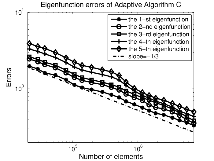
Refer to caption
Refer to caption
Figure 19: The a posteriori error estimates of the eigenpair approximations by Adaptive Algorithm CC and direct AFEM for Example 4 with the linear element

Furthermore, we also test Adaptive Algorithm CC for the smallest 55 eigenvalue and their associated eigenfunctions. Figure 19 shows the a posteriori error estimators produced by Adaptive Algorithm CC and direct AFEM with the linear finite element method. In these cases, Adaptive Algorithm CC only solve the small scale eigenvalue problems on the low dimensional space VH+span⁡{uk}V_{H}+{\rm span}\{u_{k}\} when the the numbers of elements are [21504,67846,173182,584308,2218702][21504,67846,173182,584308,2218702] (k=1,5,8,12,17k=1,5,8,12,17 and jk=1,1,1,1,1j_{k}=1,1,1,1,1).

6 Concluding remarks

In this paper, we present an efficient AFEM for eigenvalue problems based on multilevel correction scheme and the adaptive refinement technique. The most important contribution of this new AFEM is that there is no eigenvalue solving in the adaptively refined meshes which need much more computation than solving the corresponding linear boundary value problems. Furthermore, the convergence and quasi-optimal complexity have also been proved based on a relation between the eigenvalue problem and the associated boundary value problem (see Theorems 3.2 and (4.1)). Some numerical experiments for both simple and multiple eigenvalue cases are provided to demonstrate the efficiency of the proposed AFEM for eigenvalue problems. It is obvious that this efficient AFEM can be extended to the nonlinear eigenvalue problems and also other type of nonlinear problems which will be our future work.

References

  • [1] Adams, R. A.: Sobolev Spaces. Academic Press, New York (1975)
  • [2] Arnold, D. N., Mukherjee, A., Pouly, L.: Locally adapted tetrahedral meshes using bisection. SIAM J. Sci. Comput. 22, 431-448 (2000)
  • [3] Babuška, I., Osborn, J. E.: Finite element-Galerkin approximation of the eigenvalues and eigenvectors of selfadjoint problems. Math. Comp. 52, 275-297 (1989)
  • [4] Babuška, I., Osborn, J. E.: Eigenvalue problems. In: Ciarlet, P.G., Lions, J.L. (eds.) Handbook of Numerical Analysis, vol. II., pp. 641-792. North Holland, Amsterdam (1991)
  • [5] Babuška, I., Rheinboldt, W. C.: Error estimates for adaptive finite element computations. SIAM J. Numer. Anal. 15, 736-754 (1978)
  • [6] Babuška, I., Vogelius, M.: Feedback and adaptive finite element solution of one-dimensional boundary value problems. Numer. Math. 44, 75-102 (1984)
  • [7] Becker, R., Rannacher, R.: An optimal control approach to a posteriori error estimation in finite element methods. Acta Numer. 10, 1-102 (2001)
  • [8] Binev, P., Dahmen, W., DeVore, R.: Adaptive finite element methods with convergence rates. Numer. Math. 97, 219-268 (2004)
  • [9] Brenner S., Scott L.: The Mathematical Theory of Finite Element Methods. Springer-Verlag, New York (1994)
  • [10] Cascon, J. M., Kreuzer, C., Nochetto, R. H., Siebert, K. G.: Quasi-optimal convergence rate for an adaptive finite element method. SIAM J. Numer. Anal. 46(5), 2524-2550 (2008)
  • [11] Chatelin, F.: Spectral Approximations of Linear Operators. Academic Press, New York (1983)
  • [12] Chen, H., Xie, H., Xu, F.: A full multigrid method for eigenvalue problems. J. Comput. Phys. 322, 747-759 (2016)
  • [13] Ciarlet, P. G., Lions, J. L. (eds.): Finite Element Methods, Volume II of Handbook of Numerical Analysis, vol. II. North Holland, Amsterdam (1991)
  • [14] Dai, X., Xu, J., Zhou, A.: Convergence and optimal complexity of adaptive finite element eigenvalue computations. Numer. Math. 110, 313-355 (2008)
  • [15] Döfler, W.: A convergent adaptive algorithm for Poisson’s equation. SIAM J. Numer. Anal. 33, 1106-1124 (1996)
  • [16] Döfler, W., Wilderotter, O.: An adaptive finite element method for a linear elliptic equation with variable coefficients. ZAMM 80, 481-491 (2000)
  • [17] Durán, R. G., Padra, C., Rodrǵuez, R.: A posteriori error estimates for the finite element approximation of eigenvalue problems. Math. Mod. Meth. Appl. Sci. 13, 1219-1229 (2003)
  • [18] Giani, S. and Graham, I. G.: A convergent adaptive method for elliptic eigenvalue problems. SIAM J. Numer. Anal. 47(2), 1067-1091 (2009)
  • [19] Heuveline, V., Rannacher, R.: A posteriori error control for finite element approximations of ellipic eigenvalue problems. Adv. Comput. Math. 15, 107-138 (2001)
  • [20] Jia, S., Xie, H., Xie, M., Xu, F.: A full multigrid method for nonlinear eigenvalue problems. Sci. China Math. 59, 2037-2048 (2016)
  • [21] Larson, M. G.: A posteriori and a priori error analysis for finite element approximations of self-adjoint elliptic eigenvalue problems. SIAM J. Numer. Anal. 38, 608-625 (2001)
  • [22] Lin, Q., Xie, H.: A multi-level correction scheme for eigenvalue problems. Math. Comp. 84, 71-88 (2015)
  • [23] Mao, D., Shen, L., Zhou, A.: Adaptive finite algorithms for eigenvalue problems based on local averaging type a posteriori error estimates. Adv. Comput. Math. 25, 135-160 (2006)
  • [24] Maubach, J.: Local bisection refinement for nn-simplicial grids generated by reflection. SIAM J. Sci. Comput. 16, 210-227 (1995)
  • [25] Mekchay, K., Nochetto, R.H.: Convergence of adaptive finite element methods for general second order linear elliplic PDEs. SIAM J. Numer. Anal. 43, 1803-1827 (2005)
  • [26] Morin, P., Nochetto, R. H., Siebert, K.: Data oscillation and convergence of adaptive FEM. SIAM J. Numer. Anal. 38, 466-488 (2000)
  • [27] Morin, P., Nochetto, R.H., Siebert, K.: Convergence of adaptive finite element methods. SIAM Rev. 44, 631-658 (2002)
  • [28] Nochetto, R. H.: Adaptive finite elementmethods for elliptic PDE. Lecture Notes of 2006 CNA Summer School. Carnegie Mellon University, Pittsburgh (2006)
  • [29] Stevenson, R.: Optimality of a standard adaptive finite element method. Found. Comput. Math. 7, 245-269 (2007)
  • [30] Stevenson, R.: The completion of locally refined simplicial partitions created by bisection. Math. Comp. 77, 227-241 (2008)
  • [31] Traxler, C. T.: An algorithm for adaptive mesh refinement in nn dimensions. Computing 59, 115-137 (1997)
  • [32] Verfüth, R.: A Riview of a Posteriori Error Estimates and Adaptive Mesh-Refinement Techniques. Wiley-Teubner, New York (1996)
  • [33] Wu, H., Chen, Z.: Uniform convergence of multigrid V-cycle on adaptively refined finite element meshes for second order elliptic problems. Sci. China Ser. A 49, 1405-1429 (2006)
  • [34] Xie, H.: A type of multilevel method for the Steklov eigenvalue problem. IMA J. Numer. Anal. 34, 592-608 (2014)
  • [35] Xie, H.: A multigrid method for eigenvalue problem. J. Comput. Phys. 274, 550-561 (2014)
  • [36] Xie, H.: A type of multi-level correction scheme for eigenvalue problems by nonconforming finite element methods. BIT Numerical Mathematics. 55(4), 1243-1266 (2015)