A Spectral-Spatial Fusion Anomaly Detection Method for Hyperspectral Imagery
Abstract
In hyperspectral, high-quality spectral signals convey subtle spectral differences to distinguish similar materials, thereby providing unique advantage for anomaly detection. Hence fine spectra of anomalous pixels can be effectively screened out from heterogeneous background pixels. Since the same materials have similar characteristics in spatial and spectral dimension, detection performance can be significantly enhanced by jointing spatial and spectral information. In this paper, a spectral-spatial fusion anomaly detection (SSFAD) method is proposed for hyperspectral imagery. First, original spectral signals are mapped to a local linear background space composed of median and mean with high confidence, where saliency weight and feature enhancement strategies are implemented to obtain an initial detection map in spectral domain. Futhermore, to make full use of similarity information of local background around testing pixel, a new detector is designed to extract the local similarity spatial features of patch images in spatial domain. Finally, anomalies are detected by adaptively combining the spectral and spatial detection maps. The experimental results demonstrate that our proposed method has superior detection performance than traditional methods.
Keywords Hyperspectral Anomaly detection Saliency weight Feature enhancement Adaptive fusion
1 Introduction
Hyperspectral images (HSI) are different from multispectral or panchromatic images, which record not only spatial distribution information of objects but also its spectral structure information. Hence, different materials can be distinguished by using their spectral features Hou et al. 2018; Hou and Li 2022. These distinctive fine spectra like human fingerprints with uniqueness have shown great potential in target detection applications Zhao et al. 2021.
However, prior knowledge of target spectrum is difficult to obtain in advance, which limits its application scenarios. In practical terms, by only analyzing spectral signals of hyperspectral images, it is possible to identify different objects. Therefore, hyperspectral imaging has shown great potential applications for various scenarios, such as scene classification Hu et al. 2017, spectral unmixing Villa et al. 2010, change detection Hou et al. 2021a; Hou et al. 2021b, target detection Zhao et al. 2021, and anomaly detection Liu et al. 2021; Hou et al. 2020, etc.. Among these applications, anomaly detection has gotten a lot of attention due to its ability to recognize objects differing from the sourrounding background only using spectral differences rather than prior spectrum Hou et al. 2021c.
Hyperspectral anomaly dection aims to identify objects of interest that are spatially or spectrally different from its surrounding. Therefore, how to effectively select and mark anomalous pixels from an entire image has become the main challenge. For this challenge, various statistical and physical models have been reported.
Assuming that background obeys multivariate Gaussian normal distribution, well-known Reed-Yu (RX) Reed and Yu 1990 algorithm is proposed, where Mahalanobis distance is calculated to measure the similarity between testing pixel and background ones. When the whole image is considered as Gaussian background model, it is called global RX (GRX) Reed and Yu 1990. If RX detector estimates background model using local statistics, it is called local RX (LRX) Molero et al. 2013. However, the background cannot be simply described with a multivariate normal distribution because of its extremely complicated distribution. Therefore, some improved RX-based methods such as weighted RX (WRX) Guo et al. 2014, linear filter RX (LFRX) Guo et al. 2014, and kernel RX (KRX) Kwon and Nasrabadi 2005 are investigated.
Compared with the above background statistics-based methods, some linear representation-based methods producing better detection performance have been proposed. For example, the collaborative representation detector (CRD) Li and Du 2014 exploiting the similarity relationship between non-anomalous pixel and background pixels had achieved satisfactory detection performance, which represented the testing pixel linearly via its neighborhood pixels. However, the outliers in background pixels could degrade the representation accuracy. To generate relatively pure background pixels, a CRD with outlier removal anomaly detector (CRDBORAD) Vafadar and Ghassemian 2017 was proposed, removing some suspected anomaly pixels. Subsequently, a CRD combined with principal component analysis (PCAroCRD) Su et al. 2018 was put forward, where principal component analysis (PCA) was used for outlier removal. Considering the contributions of spatial information, a CRD-based local summation and inverse distance weight detector (LSADCRIDW) Tan et al. 2019a was proposed to makes full use of the various local spatial distribution information of the neighboring pixels. Utilizing the least squares technique to purify background pixels as well as weighting the average saliency of the neighboring pixels into the detection map, CRD with background purification and saliency weight [10] (CRDBPSW) was put forward.
The third anomaly detection method, as the low-rank matrix decomposition serves as a powerful tool to exploit the intrinsic low-rank property of images Candès et al. 2011. These low rank representation (LRR)-based methods aim to find a low-dimensional subspace to represent the entire image with as few as possible atoms. Assume that the background pixel obeied a single subspace, the classical robust principal component analysis (RPCA) Candès et al. 2011 method that decomposed the image matrix into a low-rank matrix and a sparse matrix, was proposed, where the sparse matrix was used for anomaly detection Liu et al. 2012. By applying the RX detector to the sparse matrix, the RPCA-RX Liu et al. 2012 detector was proposed to perform anomaly detection. Different from RPCA, the LRR model used multiple subspaces to represent the data, with being more suitable for an HSI with complex background features. Subsequently, by adding a sum-to-one constraint, the low-rank representation sum-to-one (LRRSTO) Xu et al. 2015a mode was proposed for anomaly detection. Considering that the direct application of LRR model was sensitive to a tradeoff parameter, the LRR-based and Learned Dictionary (LRRaLD) Niu and Wang 2016 method was proposed, where the dictionary was learned from the entire image with a random selection processing. To make full use of the local background statistics information, single/multiple local windows-based LRRSTO (SLW/MLW_LRRSTO) Tan et al. 2019b method was proposed. As yet, many LRR-based methods, such as sparse representation (SRD) Chen et al. 2011, low-rank and sparse representation (LRASR) Xu et al. 2015b, and graph total variation regularized low rank representation (GTVLRR) Cheng and Wang 2019, etc. have been published with better detection results.
Recently, deep learning-based methods have drawn increasing attention in hyperspectral anomaly detection. A transferred deep convolutional neural network detector (CNND) Li et al. 2017 was the first attempt to train an anomaly detector using pixel pairs selected from a reference data. With the birth of autoencoders (AEs), various AEs such as spectral constrained adversarial AE (SC_AAE) Xie et al. 2019, stacked denoising AEs (SDAs) Zhao and Zhang 2018, and manifold-constrained AE network Lu et al. 2019, etc. were introduced into hyperspectral anomaly detetion Wang et al. 2022; Zhao et al. 2017. They usually achieved outstanding judge for anomalous pixels via the spectral signal; nevertheless, the spatial features were ignored.
To address the above problems, an effective spectral-spatial fusion anomaly detection (SSFAD) framework is designed in this papar. In the spectral domain, a local median-mean line (LMML) projection method is proposed, where local adjacent pixels surrounding the testing pixel are mapped into the median-mean line to rectify the position of the background samples. In addition, a monotonic increasing function based on inverse distance weight (IDW) Tan et al. 2019a is used to further increase the gap between the anomalous and the local background pixels. The spectral feature map is obtained by a saliency weight-based detector. In the spatial domain, a local spatial similarity measurement method is proposed to fully use of spatial similarity features of local background. Finally, an adaptive score strategy is proposed to determine the fusion coefficients of the two complementary parts.
The main contributions can be summarized as follows.
1) A novel dual-pipeline framework is proposed for hyperspectral anomaly detection, where spectral and spatial features are fused by the proposed adaptive score strategy to further highlight anomaly.
2) In spectral domain, LMML projection and feature enhancement strategies were proposed to increase the discrimination between anomalious and background pixels.
3) When extracting spatial features, a local spatial similarity measurement method is designed to improve the detection effect by exploiting intrinsic local pixels relation.
The remainder of this article is organized as follows. In Section II, a detailed description of the proposed framework is presented. In Section III, four real datasets are utilized to verify the proposed method, and the parameters and results are analyzed and discussed. The conclusion is drawn in Section IV.
2 Proposed Detection Method
During background modeling in traditional methods, anomalous pixels are judged by the spectral signals, while the spatial features were ignored. Homogeneous pixels in the background may affect the detection performance. Thus, it is necessary to maximize the spatial texture between background and anomaly. Fig. 1 displays a flowchart of the proposed SSFAD framework, which consists of the following steps. To begin, spectral feature map is obatined by LMML, feature enhancement and saliency weight strategies. After that, spatial feature map is extracted by local spatial similarity measurement. Finally, two complementary detection maps are adaptive fused to highlight anomaly.

2.1 Spectral Domain-Based Anomaly Feature Extraction

In anomaly detection, covariance statistic-based methods rely excessively on the accuracy of background statistics. In hyperspectral imaging, the spectral curve is easily disturbed by various complex factors such as noise and dark current causing the oscillation of spectral curves. Moreover, in real scenarios, anomalous targets play outlier roles to contaminate the background data, which hinders the accurate estimation of the background pixels. Both phenomena could seriously degrade the performance of covariance statistic-based anomaly detection methods. In this paper, to degrade the negative effect on the mean and covariance matrix caused by anomalious pixels Imani 2017, a LMML projection method is proposed to rectify the position of background samples. Specifically, all the neighborhood pixels inside the outer window of testing pixel are projected into LMML space.
| (1) |
where and are the median value and mean value, respectively. [0, 1] denotes the position parameter. , which represents the number of pixels in the local window centered on the testing pixel . As shown in Fig. 2, the connecting line between pixel and its projection point is perpendicular to the median-mean line. According to the geometric theory, there is,
| (2) |
then,
| (3) |
After the LMML operation, local pixels are mapped in the median-mean direction, while outliers are distributed in sides of the median-mean line. The farther away from the median and mean points, the higher the probability of anomalies. Furthermore, an adaptive lcoal background prototype is obtained via the LMML projection, where the projection point of each pixel is used as the rectified background pixels to calculate the local covariance matrix.
Inspired by Lei et al. 2019, where a suppression function is used to construct a discriminative feature space. Hence, to further enlarge the difference between background and anomalous pixels, a novel monotonic increasing function is proposed, which is formulated as,
| (4) |
where and represent the projection vectors of the testing pixel and its neighborhood pixels between the outer window and the inner window in LMML space, respectively. , which is the number of neighborhood pixels. IDW denotes the inverse distance weight Tan et al. 2019a, which is used to make the most of the space-varying information where the closer the testing pixel is, the higher the similarity between the background pixels and the testing pixel will be. It is formulated as,
| (5) |
where and denote the geometric coordinates of testing pixel and its any neighborhood pixel , respectively. The feature map in spectral domain is obtained by,
| (6) |
where denotes the covariance matrix of the local background pixels between the inner window and the outer window.
In addition, considering the influence of adjacent pixels contained in an inner window on the testing pixel, a saliency weight Hou et al. 2021c is used,
| (7) |
where denotes the saliency distance between the testing pixel and its any neighborhood pixel contained in the inner window. is the number of adjacent pixels contained in the inner window. c is a constant that could cause little effect on the result. As suggested by Hou et al. 2021c, its value is set to 1. and represent the spectral distance and position distance respectively, which are formulated as,
| (8) |
| (9) |
Finally, average all saliency distances to produce the saliency weight of the testing pixel,
| (10) |
When the spectral signal of testing pixel is significantly different from that of its adjacent pixels, the pixel is regional saliency. Therefore, the final detection result in spectral domain is reformulated as,
| (11) |
2.2 Spatial Domain-Based Anomaly Feature Extraction
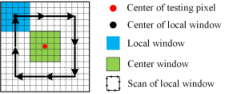
If the testing pixel is anomalous, its saptial structure would differ from ones of the neighborhood background Ju et al. 2018. To calculate the spatial structure similarity between the testing pixel and its neighborhood background, a novel local spatial similarity measurement method is formulated as,
| (12) |
where denotes the center window (see the green window in Fig. 3) centered on testing pixel, is the neighborhood background window (highlighted as the blue window in Fig. 3), and represents the size of spatial structure window.
The local spatial similarity of the center window is calculated following Fig. 3. By sliding the blue window clockwise around the green window, the local spatial similarity information around the center window is obtained. Theoretically, different sizes and shapes should be selected for the spatial structure window for a better adaption to the local characteristics in images. For simplicity, the inner green window is regarded as the spatial structure window. In addition, the size of local background window is set as . The most similar spatial structure window are searched from its background area. By Eq. 12, the spatial structure similarity between center window around testing pixel and its neighborhood background windows is obtained. The bigger the similarity, the smaller the value, and the more likely it is to be background, and vice versa.
2.3 Spectral-Spatial Fusion Anomaly Detection
To highlight anomalous targets, two complementary detection maps are adaptively fused. Single feature cannot detect anomaly well in complex scenario, therefore, a fusion strategy is adopted here. A linear score function shown in Eq.13 is employed as the fusion strategy.
| (13) |
where is the finally anomaly detection result. and are the corresponding weight factors. It is difficult to tune and experiencelly to obtain an optimal value, and a general option is the average pooling operation. That is, . In this paper, a score mechanism is proposed to adaptively determine the values of and , which is formulated as,
| (14) |
where takes the maximal eigenvalue of an matrix. Such adaptive score strategy could help to increase the detection performance.


3 Experiments and Discussion
3.1 Datasets Description
In this section, to evaluate the performance of the proposed detector, experiments are conducted on four hyperspectral images. The first image Kang et al. 2017 was obtained by airborne visible/infrared imaging spectrometer (AVIRIS) sensor over Gulfport area on July 7, 2010. This Gulfport image with spatial resolution of 3.4 m, consists of 100 100 pixels and 191 spectral bands after removing the invalid bands, where the anomalies refer to the airplanes. The scenario and its ground-truth map are shown in Fig. 4(a) and Fig.4(e).
The second image Kang et al. 2017; Bitar et al. 2019 was acquired by the Reflective Optics System Imaging Spectrometer (ROSIS) airborne sensor during a flight campaign over Pavia, northern Italy. Its size and geometric resolution are 150 150 115 and 1.3 m, respectively. 102 bands are retained as the noisy bands are discarded. The Pavia Centra image mainly contains a background of water and a bridge and some anomalies of vehicles, of which the scenario and the ground-truth map are given in Fig. 4(b) and Fig. 4(f).
The third dataset Kang et al. 2017 of spatial resolution 3.5 m is an urban scene of Gainesville located on the north central of Florida, USA, obtained by AVIRIS on September 4, 2010. It consists of 191 image bands of size 100 100. Fig. 4(c) and Fig. 4(g) depict the Gainesville image and its corresponding ground truth, respectively.
The fourth dataset Huyan et al. 2018; Zhang et al. 2015 was acquired by the Nuance Cri Hyperspectral sensor at the spectral resolution of 10 m and in the wavelength range of [650, 1100] nm. The Cri image of size 400 400 46 captures a grassland corrupted by 10 rock anomalies of pixel 2261. The pseudo color image is shown in Fig. 4(d), while the contained anomalies can be clearly observed in Fig. 4(h).


| Methods | Gulfport | Pavia Centra | Gainesville | Cri |
|---|---|---|---|---|
| LRX | (17,15) | (25,5) | (9,7) | (19,15) |
| CRD | (23,15,) | (7,5,) | (9,7,) | (19,9,) |
| RPCA-RX | 0.01 | 0.01 | 0.01 | 0.001 |
| GTVLRR | (0.5,0.2,0.1) | (0.7,0.4,0.05) | (0.005,1,0.5) | (0.005,1,0.5) |
| 2S-GLRT | (13,11) | (21,5) | (9,5) | (25,15) |
| SSFAD | (5,3) | (5,3) | (5,3) | (17,15) |
| Methods | Gulfport | Pavia Centra | Gainesville | Cri |
|---|---|---|---|---|
| average pooling | 99.309 | 99.843 | 98.903 | 99.614 |
| adaptive score | 99.307 | 99.882 | 98.970 | 99.751 |
3.2 Parameters setting
To effectively verify the performance of the proposed SSFAD method, six widely-used anomaly detectors, e.g. GRX, LRX, CRD, RPCA-RX, GTVLRR and 2S-GLRT, are employed for evaluation. Meanwhile, for qualitative and quantitative comparisons, statistical separability analysis Hou et al. 2021c, receiver operating characteristic (ROC) Hanley and McNeil 1982 and area under the curve (AUC) metric are utilized as the main criteria.
The choices of parameters are important for these methods with parameters, by which its detection performance is greatly affected. For a fair comparison, the parameters of all considered methods are carefully tuned following their expriences, to generate their best detection results. As suggested in Liu et al. 2021; Hou et al. 2021c, for the LRX and SSFAD, by varying the outer window size from 5 to 25 and the inner window size from 3 to 15, the optimal detection performance under different window sizes is collected. For the CRD, by fixing as and varying from 5 to 25 and from 3 to 15, the optimal detection performance under different window sizes is selected. For the RPCA-RX, the optimal parameter is selected from to for comparative experiments. As to the GTVLRR, the K-means method is used to construct dictionary referring to Cheng and Wang 2019; Liu et al. 2021, and empirical parameters (, , ) are firstly set to (0.5, 0.2, 0.05). Then, by fixing and , and varying in [0.005, 0.05, 0.1, 0.3, 0.5, 0.7, 1], the optimal under different values is selected. Similarly, by fixing the selected and default , and varying in [0.005, 0.05, 0.1, 0.2, 0.4, 0.7, 1], the optimal is selected. In the same way, the optimal is selected in [0.005, 0.01, 0.02, 0.05, 0.1, 0.2, 0.5]. The optimal parameters of various detectors are listed in Table 1.
| Methods | Gulfport | Pavia Centra | Gainesville | Cri |
|---|---|---|---|---|
| GRX | 95.260 | 95.380 | 95.128 | 91.342 |
| LRX | 96.942 | 95.973 | 97.690 | 75.251 |
| CRD | 97.927 | 94.072 | 93.930 | 87.267 |
| RPCA-RX | 95.348 | 95.906 | 95.861 | 91.478 |
| GTVLRR | 99.691 | 97.636 | 88.604 | 93.429 |
| 2S-GLRT | 91.831 | 98.676 | 94.856 | 95.403 |
| SSFAD | 99.307 | 99.882 | 98.970 | 99.751 |
| Methods | Gulfport | Pavia Centra | Gainesville | Cri |
|---|---|---|---|---|
| GRX | 0.08 | 0.08 | 0.12 | 0.32 |
| LRX | 39.57 | 50.98 | 34.14 | 91.59 |
| CRD | 69.97 | 4.79 | 3.87 | 866.59 |
| RPCA-RX | 2.61 | 2.19 | 2.56 | 7.76 |
| GTVLRR | 61.06 | 88.89 | 49.40 | 981.47 |
| 2S-GLRT | 74.36 | 48.11 | 36.60 | 4272.53 |
| SSFAD | 50.44 | 44.67 | 47.67 | 3197.97 |
3.3 Detection Performance
Statistical separability analysis Liu et al. 2021; Zhao et al. 2021, also known as boxplot, has been widely used as a performance assessment in hyperspectral anomaly detection, target detection, and change detection. Essentially, the boxplot is used to reflect the distribution characteristics of various detection results, where the separation degree between different categories is judged by the interval between different boxes. Herein, the separability and the suppression level between anomaly and background is evaluated by statistical separability analysis, where the red and green boxes represent the anomalous and background pixels, respectively. The interval between the red and green box represents the separability between the anomalous and background pixels, while the height of the green box means the suppression degree of these methods to the background. Generally, a shorter green box corresponds to a stronger background suppression, refelcting a better separation for background and anomaly.
The detection performance of the considered algorithms on four experimental datasets is displayed. As can be seen from Fig. 5(a) that the intervals between the red and green boxes of SSFAD and GTVLRR are larger than those of the GRX, LRX, CRD, RPCA-RX and 2S-GLRT, which indicates that both methods can separate the anomalies well from the background. In addition, SSFAD is sightly better than GTVLRR towards interval, and perform the shortest green box. Thus, this proposed method can suppress the background better in the Gulfport dataset. Fig. 5(b) shows that except CRD, the compared detectors can effectively suppress the background of the Pavia Centra dataset. Obviously, SSFAD achieves the best separability than the others. From Fig. 5(c) and Fig. 5(d), it can be seen that SSFAD produces the widest interval when compared with other six detectors, i.e., GRX, LRX, CRD, RPCA-RX, GTVLRR and 2S-GLRT. Comprehensively, the proposed SSFAD can separate anomalies from background more effectively.
For an accuracy evaluation, the ROC curves of each detector on the experimental images are plotted in Fig. 6. The closer the curve is to the upper left corner, the better the detection performance. As Fig. 6(a) depicted, the GRX shows the worst performance. The green and black curves are closer to the upper left corner than others, representing that GTVLRR and the proposed SSFAD both achiev good detection performance, and GTVLRR is slightly better than SSFAD. The experimental results shown in Figs. 6(b)-(d) reveal the obvious advantage of the proposed SSFAD when detecting the Pavia Centra, Gainesville, and Cri dataset, because the black curve is closest to the upper left corner.
The AUC values of different fusion strategies are compared in Table 2. Obviously, the proposed adaptive score strategy achieves better results than the average pooling strategy, especially in Cri dataset. This also further confirms that the adaptive score stategy can better highlight anomaly than the average pooling strategy. In addition, the AUC values of various methods on differet datasets are listed in Table 3. By comparing these AUC values, the almost best performance of proposed SSFAD can be observed. Especially on the Cri dataset, the improvement of SSFAD approximates to 4% when compared with the second best detector. Table 4 provides the execution time of the compared methods, where the mediocre time performance of the proposed SSFAD is exposed. Such unideal time consuming probably is caused by the computational cost of matrix inversion operation and saliency weight calculation increasing with the size of the additional local window. Whatever, the ordinary time performance can hardly cover the superiorities of the proposed SSFAD towards hyperspectaral anomaly detection.
4 Conclusions
In this paper, a novel dual-pipeline framework that extracted spatial and spectral features separately and then fused them adaptively was proposed for hyperspectral anomaly detection. In spectral domain, original spectral signal was first mapped to a local median-mean linear background, and then saliency weight and feature enhancement strategies were implemented to obtain an initial detection map. In spatial domain, a new detector was designed to fully excavate the similarity spatial information of local patches around center window. Finally, anomalies were detected by jointly considering the spectral and spatial detection maps. Experimental results on four real hyperspectral datasets confirmed that the proposed SSFAD method had superior background suppression ability and excellent detection performance than traditional anomaly detection methods.
References
- Hou et al. [2018] Zengfu Hou, Yu Chen, Kun Tan, and Peijun Du. Novel hyperspectral anomaly detection methods based on unsupervised nearest regularized subspace. International Archives of the Photogrammetry, Remote Sensing & Spatial Information Sciences, 42(3), 2018.
- Hou and Li [2022] Zengfu Hou and Wei Li. A joint morphological profiles and patch tensor change detection for hyperspectral imagery. arXiv preprint arXiv:2201.08027, 2022.
- Zhao et al. [2021] Xiaobin Zhao, Zengfu Hou, Xin Wu, Wei Li, Pengge Ma, and Ran Tao. Hyperspectral target detection based on transform domain adaptive constrained energy minimization. International Journal of Applied Earth Observation and Geoinformation, 103:102461, 2021.
- Hu et al. [2017] Jingliang Hu, Lichao Mou, Andreas Schmitt, and Xiao Xiang Zhu. Fusionet: A two-stream convolutional neural network for urban scene classification using polsar and hyperspectral data. In 2017 Joint Urban Remote Sensing Event (JURSE), pages 1–4. IEEE, 2017.
- Villa et al. [2010] Alberto Villa, Jocelyn Chanussot, Jon Atli Benediktsson, and Christian Jutten. Spectral unmixing for the classification of hyperspectral images at a finer spatial resolution. IEEE Journal of Selected Topics in Signal Processing, 5(3):521–533, 2010.
- Hou et al. [2021a] Zengfu Hou, Wei Li, Lu Li, Ran Tao, and Qian Du. Hyperspectral change detection based on multiple morphological profiles. IEEE Transactions on Geoscience and Remote Sensing, 2021a.
- Hou et al. [2021b] Zengfu Hou, Wei Li, Ran Tao, and Qian Du. Three-order tucker decomposition and reconstruction detector for unsupervised hyperspectral change detection. IEEE Journal of Selected Topics in Applied Earth Observations and Remote Sensing, 14:6194–6205, 2021b.
- Liu et al. [2021] Jun Liu, Zengfu Hou, Wei Li, Ran Tao, Danilo Orlando, and Hongbin Li. Multipixel anomaly detection with unknown patterns for hyperspectral imagery. IEEE Transactions on Neural Networks and Learning Systems, pages 1–11, 2021. doi:10.1109/TNNLS.2021.3071026.
- Hou et al. [2020] Zengfu Hou, Wei Li, Lianru Gao, Bing Zhang, Pengge Ma, and Junling Sun. A background refinement collaborative representation method with saliency weight for hyperspectral anomaly detection. In IGARSS 2020-2020 IEEE International Geoscience and Remote Sensing Symposium, pages 2412–2415. IEEE, 2020.
- Hou et al. [2021c] Zengfu Hou, Li Wei, Ran Tao, and Weihua Shi. Collaborative representation with background purification and saliency weight for hyperspectral anomaly detection. SCIENCE CHINA Information Sciences, 65:112305, 2021c.
- Reed and Yu [1990] Irving S Reed and Xiaoli Yu. Adaptive multiple-band cfar detection of an optical pattern with unknown spectral distribution. IEEE Transactions on Acoustics, Speech, and Signal Processing, 38(10):1760–1770, 1990.
- Molero et al. [2013] José Manuel Molero, Ester M Garzón, Inmaculada García, and Antonio Plaza. Analysis and optimizations of global and local versions of the rx algorithm for anomaly detection in hyperspectral data. IEEE Journal of Selected Topics in Applied Earth Observations and Remote Sensing, 6(2):801–814, 2013.
- Guo et al. [2014] Qiandong Guo, Bing Zhang, Qiong Ran, Lianru Gao, Jun Li, and Antonio Plaza. Weighted-rxd and linear filter-based rxd: Improving background statistics estimation for anomaly detection in hyperspectral imagery. IEEE Journal of Selected Topics in Applied Earth Observations and Remote Sensing, 7(6):2351–2366, 2014.
- Kwon and Nasrabadi [2005] Heesung Kwon and Nasser M Nasrabadi. Kernel rx-algorithm: A nonlinear anomaly detector for hyperspectral imagery. IEEE transactions on Geoscience and Remote Sensing, 43(2):388–397, 2005.
- Li and Du [2014] Wei Li and Qian Du. Collaborative representation for hyperspectral anomaly detection. IEEE Transactions on Geoscience and Remote Sensing, 53(3):1463–1474, 2014.
- Vafadar and Ghassemian [2017] Maryam Vafadar and Hassan Ghassemian. Hyperspectral anomaly detection using outlier removal from collaborative representation. In 2017 3rd International Conference on Pattern Recognition and Image Analysis (IPRIA), pages 13–19. IEEE, 2017.
- Su et al. [2018] Hongjun Su, Zhaoyue Wu, Qian Du, and Peijun Du. Hyperspectral anomaly detection using collaborative representation with outlier removal. IEEE Journal of Selected Topics in Applied Earth Observations and Remote Sensing, 11(12):5029–5038, 2018.
- Tan et al. [2019a] Kun Tan, Zengfu Hou, Fuyu Wu, Qian Du, and Yu Chen. Anomaly detection for hyperspectral imagery based on the regularized subspace method and collaborative representation. Remote sensing, 11(11):1318, 2019a.
- Candès et al. [2011] Emmanuel J Candès, Xiaodong Li, Yi Ma, and John Wright. Robust principal component analysis? Journal of the ACM (JACM), 58(3):1–37, 2011.
- Liu et al. [2012] Guangcan Liu, Zhouchen Lin, Shuicheng Yan, Ju Sun, Yong Yu, and Yi Ma. Robust recovery of subspace structures by low-rank representation. IEEE transactions on pattern analysis and machine intelligence, 35(1):171–184, 2012.
- Xu et al. [2015a] Yang Xu, Zebin Wu, Zhihui Wei, Hongyi Liu, and Xiong Xu. A novel hyperspectral image anomaly detection method based on low rank representation. In 2015 IEEE International Geoscience and Remote Sensing Symposium (IGARSS), pages 4444–4447. IEEE, 2015a.
- Niu and Wang [2016] Yubin Niu and Bin Wang. Hyperspectral anomaly detection based on low-rank representation and learned dictionary. Remote Sensing, 8(4):289, 2016.
- Tan et al. [2019b] Kun Tan, Zengfu Hou, Donglei Ma, Yu Chen, and Qian Du. Anomaly detection in hyperspectral imagery based on low-rank representation incorporating a spatial constraint. Remote Sensing, 11(13):1578, 2019b.
- Chen et al. [2011] Yi Chen, Nasser M Nasrabadi, and Trac D Tran. Simultaneous joint sparsity model for target detection in hyperspectral imagery. IEEE Geoscience and Remote Sensing Letters, 8(4):676–680, 2011.
- Xu et al. [2015b] Yang Xu, Zebin Wu, Jun Li, Antonio Plaza, and Zhihui Wei. Anomaly detection in hyperspectral images based on low-rank and sparse representation. IEEE Transactions on Geoscience and Remote Sensing, 54(4):1990–2000, 2015b.
- Cheng and Wang [2019] Tongkai Cheng and Bin Wang. Graph and total variation regularized low-rank representation for hyperspectral anomaly detection. IEEE Transactions on Geoscience and Remote Sensing, 58(1):391–406, 2019.
- Li et al. [2017] Wei Li, Guodong Wu, and Qian Du. Transferred deep learning for anomaly detection in hyperspectral imagery. IEEE Geoscience and Remote Sensing Letters, 14(5):597–601, 2017. doi:10.1109/LGRS.2017.2657818.
- Xie et al. [2019] Weiying Xie, Jie Lei, Baozhu Liu, Yunsong Li, and Xiuping Jia. Spectral constraint adversarial autoencoders approach to feature representation in hyperspectral anomaly detection. Neural Networks, 119:222–234, 2019.
- Zhao and Zhang [2018] Chunhui Zhao and Lili Zhang. Spectral-spatial stacked autoencoders based on low-rank and sparse matrix decomposition for hyperspectral anomaly detection. Infrared Physics & Technology, 92:166–176, 2018.
- Lu et al. [2019] Xiaoqiang Lu, Wuxia Zhang, and Ju Huang. Exploiting embedding manifold of autoencoders for hyperspectral anomaly detection. IEEE Transactions on Geoscience and Remote Sensing, 58(3):1527–1537, 2019.
- Wang et al. [2022] Shaoyu Wang, Xinyu Wang, Liangpei Zhang, and Yanfei Zhong. Auto-ad: Autonomous hyperspectral anomaly detection network based on fully convolutional autoencoder. IEEE Transactions on Geoscience and Remote Sensing, 60:1–14, 2022. doi:10.1109/TGRS.2021.3057721.
- Zhao et al. [2017] Chunhui Zhao, Xueyuan Li, and Haifeng Zhu. Hyperspectral anomaly detection based on stacked denoising autoencoders. Journal of Applied Remote Sensing, 11(4):042605, 2017.
- Imani [2017] Maryam Imani. Rx anomaly detector with rectified background. IEEE Geoscience and Remote Sensing Letters, 14(8):1313–1317, 2017.
- Lei et al. [2019] Jie Lei, Weiying Xie, Jian Yang, Yunsong Li, and Chein-I Chang. Spectral–spatial feature extraction for hyperspectral anomaly detection. IEEE Transactions on Geoscience and Remote Sensing, 57(10):8131–8143, 2019.
- Ju et al. [2018] Huihui Ju, Zhigang Liu, and Yang Wang. Hyperspetral anomaly detection incorporating spatial information. In 2018 Eighth International Conference on Image Processing Theory, Tools and Applications (IPTA), pages 1–5. IEEE, 2018.
- Kang et al. [2017] Xudong Kang, Xiangping Zhang, Shutao Li, Kenli Li, Jun Li, and Jon Atli Benediktsson. Hyperspectral anomaly detection with attribute and edge-preserving filters. IEEE Transactions on Geoscience and Remote Sensing, 55(10):5600–5611, 2017.
- Bitar et al. [2019] Ahmad W Bitar, Loong-Fah Cheong, and Jean-Philippe Ovarlez. Sparse and low-rank matrix decomposition for automatic target detection in hyperspectral imagery. IEEE Transactions on Geoscience and Remote Sensing, 57(8):5239–5251, 2019.
- Huyan et al. [2018] Ning Huyan, Xiangrong Zhang, Huiyu Zhou, and Licheng Jiao. Hyperspectral anomaly detection via background and potential anomaly dictionaries construction. IEEE Transactions on Geoscience and Remote Sensing, 57(4):2263–2276, 2018.
- Zhang et al. [2015] Yuxiang Zhang, Bo Du, Liangpei Zhang, and Shugen Wang. A low-rank and sparse matrix decomposition-based mahalanobis distance method for hyperspectral anomaly detection. IEEE Transactions on Geoscience and Remote Sensing, 54(3):1376–1389, 2015.
- Hanley and McNeil [1982] James A Hanley and Barbara J McNeil. The meaning and use of the area under a receiver operating characteristic (roc) curve. Radiology, 143(1):29–36, 1982.