Training Characteristic Functions with Reinforcement Learning:
XAI-methods play Connect Four

Stephan Wäldchen¹¹ 1 Both authors contributed equally to this work. waeldchen@zib.de Affiliation: Institute of Mathematics & AI in Society, Science, and Technology Affiliation: Technische Universität Berlin & Zuse Institute Berlin Affiliation: Berlin, Germany Felix Huber¹¹ 1 Both authors contributed equally to this work. huber@zib.de Affiliation: Institute of Mathematics & AI in Society, Science, and Technology Affiliation: Technische Universität Berlin & Zuse Institute Berlin Affiliation: Berlin, Germany Sebastian Pokutta pokutta@zib.de Affiliation: Institute of Mathematics & AI in Society, Science, and Technology Affiliation: Technische Universität Berlin & Zuse Institute Berlin Affiliation: Berlin, Germany

Abstract

Characteristic functions (from cooperative game theory) are able to evaluate partial inputs and form the basis for attribution methods like Shapley values. These attribution methods allow us to measure how important each input component is for the function output—one of the goals of explainable AI (XAI). Given a standard classifier function, it is unclear how partial input should be realised. Instead, most XAI-methods for black-box classifiers like neural networks consider counterfactual inputs that generally lie off-manifold, which makes them hard to evaluate and easy to manipulate.

We propose a setup to directly train characteristic functions in the form of neural networks to play simple two-player games. We apply this to the game of Connect Four by randomly hiding colour information from our agents during training. This has three advantages for comparing XAI-methods: It alleviates the ambiguity about how to realise partial input, makes off-manifold evaluation unnecessary and allows us to compare the methods by letting them play against each other.

1 Introduction

The safe deployment of AI-systems in high-stakes applications such as autonomous driving Schraagen et al., 2020, medical imaging Holzinger et al., 2017 and criminal justice Rudin and Ustun, 2018 requires that their decisions can be subjected to human scrutiny. The most successful models, often based on machine learning (ML) and deep neural networks (DNN), have instead grown increasingly complex and are widely regarded to operate as black-boxes. This spawned the field of explainable AI (XAI) with the explicit aim to make ML models transparent in their reasoning.

1.1 Explainable Artificial Intelligence

Though XAI had practical success, such as detecting biases in established data sets Lapuschkin et al., 2019, there is currently no consensus among researchers about what exactly constitutes an explainable model Lipton, 2018. For a good overview see Adadi and Berrada, 2018.

Models such as $k$ -nearest neighbours, succinct decision trees or sparse linear models are deemed inherently interpretable Arrieta et al., 2020, which makes them preferable Rudin, 2019. However, the most impressive breakthroughs in the field of AI have only been possible with DNNs. In this light, a second paradigm emerged: to apply these successful models and explain them post-hoc.

In this work, we focus on saliency (or relevance) attribution methods. Given a classifier and input, these methods rate the importance of each feature for the classifier output, often displayed visually as a heatmap, called a saliency map. We give an overview over the proposed methods in Section 2.

1.2 Characteristic Functions

Cooperative game theory considers attribution problems very similar to saliency attribution, where a common pay-off is to be fairly distributed to a number of cooperating players. In the context of ML, players correspond to features and the pay-off is the classifier score. Let $d\in\mathbb{N}$ be the number of features, and $[d]=\mathopen{}\left\{1,\dots,d\right\}\mathclose{}$ . One key concept is the characteristic function $\nu\colon 2^{[d]}\rightarrow\mathbb{R}$ which assigns a value to every possible subset $S$ of the $d$ features, called a coalition. We refer the reader to Chalkiadakis et al., 2011 for a good introduction into cooperative game theory.

For binary classifiers this led to the concept of prime implicant explanations (PIE) that search for the smallest coalition $S\subset[d]$ that ensures a value of $\nu(S)=1$ , see Shih et al., 2018. These explanations can be efficiently computed for certain simple classifiers like decision trees or binary decision diagrams.

Furthermore, the Shapley values are an established attribution method, defined as

\phi_{\nu,i}=\sum_{S\subseteq[d]\setminus\{i\}}\begin{pmatrix}d-1\\ \mathopen{}\left|S\right|\mathclose{}\end{pmatrix}^{-1}\mathopen{}\left(\nu(S\cup\{i\})-\nu(S)\right)\mathclose{}.

Shapley values are the unique attribution methods that satisfy certain desirable fairness criteria, see Shapley, 2016 and Appendix E.

Both PIE and Shapley values are thus defined over desirable properties, and the actual algorithm to compute them depends on the model. In contrast, most saliency attribution methods for neural networks are defined directly over algorithmic instructions and lack definite properties that make them useful¹¹ 1 Except the gradient maps, though these suffer from other shortcomings as explained in Appendix A. Even the saliency methods that are inspired by PIE and Shapley values (see Section 2) do not maintain their desirable theoretical properties while at the same being computationally efficient Macdonald et al., 2020. This means that the only way to judge whether these saliency methods have merit is to evaluate them in practical scenarios.

1.3 Evaluating Saliency Methods

Figure 1: Connect 4 with missing colour information shown in grey. a) A game between two pairs of maskers and players. The maskers decide which colour information to pass on to the players with an upper limit of revealing half the played pieces. The player has to decide his move based on the information sent by the masker. Our the players are both represented by the same policy network. Which information to reveal will later be chosen by different saliency methods. b) The game board is encoded in three input channels: Two binary matrices indicating the pieces of each player and one indicate the open fields. With full information the encoding is redundant, with only partial information the agent is unsure about the colour of some pieces but can still make valid moves.

In Doshi-Velez and Kim, 2017 the authors differentiate between human-based and functionally-grounded evaluation. The former has the advantage of measuring directly what we want, namely that explanations are legible and helpful to humans. On the other hand, human-based evaluations are costly and hard to generalise from one task to another. They also cannot discern between a network with unintuitive reasoning and a saliency method that produces unintuitive results. Functionally grounded evaluation aims to design proxy tasks whose success is correlated with the quality of the explanation. They often ask, which information is useful to the interpreted network itself, see Mohseni et al., 2021, so that only the quality of the saliency method matters. This approach also allows for much larger scale experiments. However, not all proxy-task are necessarily linked to good explanations Biessmann and Refiano, 2021.

The proxy task we consider here is: successful play of abstract games with limited information. In our case study we investigate the game Connect Four Allis, 1988. We make use of the fact that neural networks have emerged as one of the strongest models for reinforcement learning, and e.g. constitute the first human competitive models for Go Silver et al., 2017 and Atari games Mnih et al., 2015.

Our exact setup is illustrated in Figure 1. A masker and a player are paired against a second team of the same form. The masker, presents a limited amount of information (colour features) to their player, who then selects the next move. The full board state is then given to the masker of the opposing team who selects the information for their player, and so on until the game is finished either by one party winning or a draw. The players are modelled by DNNs without memory and base their decision only on the information currently provided by the masker. During training, the masker will select information randomly up to a varying maximal amount. For the comparison of the saliency methods, the masker will instead be represented by a method that explains the move that the player would have made given full information. The most salient features are then given to the player for their actual move.

1.4 Our Contribution

First, we give an overview over the existing saliency methods and explain how they are vulnerable to manipulation if they rely on off-manifold inputs. We show that for image obfuscation, one of the most used evaluation metrics, the best-performing methods give artefactual explanations that rely on “superstimuli”, a phenomenon resulting from evaluating classifiers off-manifold.

As a remedy, we directly train agents as characteristic functions for reinforcement learning, by randomly hiding colour features and show that this setup delivers results comparable to training solely on full information. Additionally, we demonstrate a relatively monotonous relationship between information and performance in the game, which justifies the setup explained in Figure 1 as a sensible proxy task for XAI methods. Since our agents can handle partial input, we can directly compute Shapley values via sampling. These are theoretically well understood and rely only on counterfactual input the agent has been trained on—which makes this sound attribution method. We demonstrate their usefulness by comparing to the ground truth available for certain board situations. Additionally, we learn that training on hidden input is not enough to ensure interpretability if the training is linked to the wrong objective.

We then compare a selection of XAI methods in a round-robin tournament in Connect Four, which has some advantages that image obfuscation comparisons generally lack:

1.

It is canonically clear how missing information should be modelled (since it is included in the training).
2.

There is no need to evaluate the classifier off-manifold.
3.

We have a concrete task (Winning the game) to compare the XAI-methods.

2 Related Work

A lot of work has been done to design methods that produce saliency maps for neural networks. So far, these methods are not equipped with theoretical guarantees that they fulfil a certain quality property, as compared to Shapley values and PIE, see Section 1.2. They are instead motivated by heuristic arguments and then numerically evaluated. We give a short overview over the existing heuristics and then explain that first, methods relying on off-manifold counterfactuals are manipulable and secondly, evaluations relying on off-manifold inputs are manipulable as well.

2.1 Saliency Methods

We restrict our analysis to local, post-hoc saliency methods for neural network classifiers, both model specific and model-agnostic. We differentiate the following three categories.

Local Linearisation

Linear methods are considered interpretable, so it is a natural approach for nonlinear models to instead interpret a local linearisation. In this category we find gradient maps Simonyan et al., 2013, SmoothGrad Smilkov et al., 2017, which samples the gradient around the input, and LIME Ribeiro et al., 2016 which applies the classifier to samples around the input then fits a new linear classifier to the resulting input-label-pairs.

Heuristic Backpropagation

These methods replace the chain-rule of gradient backpropagation with different heuristically motivated rules and propagate relevance scores back to the input. One of the earliest methods methods for neural networks was deconvolution Zeiler and Fergus, 2014, newer methods include GuidedBackpropagation (GB) Springenberg et al., 2015, DeepLift Shrikumar et al., 2017, DeepShap Lundberg and Lee, 2017a and LRP Bach et al., 2015. These methods have the advantage of being computationally very fast and applicable in real-time.

Partial Input

These methods rely on turning a classifier function $f$ and an input $\mathbf{x}$ into a characteristic function $\nu_{f,\mathbf{x}}$ . The standard way to define $\nu_{f,\mathbf{x}}(S)$ for a feature set $S$ , put forth by Lundberg and Lee, 2017b, is to regard the missing features $\mathbf{x}_{S^{c}}$ as random variables and take an expectation value conditioned on the given parameters $\mathbf{x}_{S}$ , i.e.

\nu_{f,\mathbf{x}}(S)=\mathbb{E}_{\mathbf{y}}\mathopen{}\left[f(\mathbf{y})\,|\,\mathbf{y}_{S}=\mathbf{x}_{S}\right]\mathclose{}=\int f(\mathbf{x})p(\mathbf{x}_{S^{c}}\,|\,\mathbf{x}_{S})\,\text{d}\mathbf{x}_{S^{c}}.

(2.1)

Being able to evaluate partial input, these methods either optimise an objective similar to prime implicant explanations, for example Rate-Distortion Explanations (RDE) Macdonald et al., 2020 and Anchors Ribeiro et al., 2018, or approximate Shapley values Sundararajan and Najmi, 2020. This however is computationally infeasible to do exactly, so these methods instead rely on heuristic strategies that do not carry over the quality properties of PIE and Shapley values. Additionally, the soundness of these heuristics depends strongly on how correctly the conditional distribution $p(\mathbf{x}_{S^{c}}\,|\,\mathbf{x}_{S})$ is modelled, as we will discuss next.

2.2 Off-Manifold Input

Refer to caption — Figure 2: RDE-Explanations of a bird image taken from Macdonald et al., 2021 with permission of the authors. The proposed optimisation methods (FW, AFW, LCG, LAFW) search for the smallest set of pixels that still maintain the classification of “bird”, if the other pixels are randomised. All produce a mask that creates a new bird head as a “superstimulus” mask. The sensitivity map does not show this behaviour. The distribution of the randomised pixels is independent from the selected set, which means the contours of the set will be visible and detectable by the pattern matching network. Modelling the noise after true distribution $p(\mathbf{x}_{S^{c}}\,|\,\mathbf{x}_{S})$ (as in Equation 2.1) would prevent this effect, since a monochrome selection of black pixels would likely be inpainted with black as well. Then no bird’s head would appear.

These post-hoc relevance methods have in common that they consider counterfactual information: “What if I would change this part of the input?”. We explain how this applies to each method in Appendix A.

For this reason, the saliency methods can all be manipulated by principally the same idea: replace an existing model by a another one that agrees on the data manifold but not off-manifold, where the behaviour can be chosen arbitrarily. This allows to hide biases in classifiers for on-manifold inputs almost at will, as demonstrated for gradient maps and integrated gradients Anders et al., 2020; Dimanov et al., 2020, LRP Anders et al., 2020; Dombrowski et al., 2019, LIME Slack et al., 2020; Dimanov et al., 2020, DeepShap Slack et al., 2020; Dimanov et al., 2020, Grad-Cam Heo et al., 2019, Shapley-basedFrye et al., 2020 and general counterfactual explanations Slack et al., 2021.

Image Obfuscation

In the absence of human annotations (such as bounding boxes or pixel-wise annotations), some functionally grounded evaluation for image data obfuscate part of the image and measure how much the classifier output changes Mohseni et al., 2021. The idea is this: keeping the relevant features intact should leave the classification stable, obfuscating them should rapidly decay the classifier score. This method was introduced as pixel-flipping Samek et al., 2017 and used to evaluate XAI-methods for image recognition Fong and Vedaldi, 2017; Macdonald et al., 2019 and Atari games Huber et al., 2021.

In Macdonald et al., 2019 the authors directly optimise for a mask that selects sparse features which maintain the classifier decision, severely outperforming competitors. In Macdonald et al., 2021 this method gets improved further with methods from convex optimisation (Frank-Wolfe optimiser). However, visually inspecting the produced saliency maps reveals they create new features that were not present in the original image. This is possible over a mechanism similar to adversarial examples, see Figure 2, which means: the optimal mask creates its own features! Since the distribution of the obfuscated part of the image is independent from the rest the created images lie off-manifold which makes this effect possible. To keep the image on-manifold, the obfuscated part would have to be sampled from the true conditional data distribution $p(\mathbf{x}_{S^{c}}\,|\,\mathbf{x}_{S})$ which is not known. This shows that proxy tasks have to be designed with care if they are meant to be useful for comparing saliency methods. Not only are the methods vulnerable to manipulation by going off-manifold, the evaluation tasks themselves can be exploited by making use of off-manifold inputs.

3 Setup

Instead of trying to turn a classifier function into a characteristic function, we propose to directly train on hidden features. Policy and value functions (see Li, 2017) for agents that play simple two-player, turn-based games (such as Go, Checkers, Hex) are particularly well suited for this task.

The logic of these games is complex enough to make the use of black-box functions such as neural network sensible, and in the case of Go the unbeaten standard. At the same time, the input is low-dimensional and discrete. Additionally, the input components have weaker correlations between neighbours, i.e. a random configuration of Connect Four pieces can still be a valid game²² 2 if the number of pieces for each player is balanced, whereas a random assortment of pixels will almost surely not be a valid image. These factors facilitate sampling partial inputs during training. ³³ 3 For image data by comparison, simply hiding random pixels would not do, since the image can likely still be inferred by inpainting.

Figure 3: Network architecture for the PPO-agent. The convolutional layers (Conv) have

3\times 3

filters, 512 channels,

1\times 1

stride and use zero-padding. The fully connected (FC) layers for the policy and value head use softmax and tanh-activation respectively. All other layers use ReLU-activations.

3.1 Hiding the Player Colour

The most straight-forward way of hiding information from an agent would be to complete hide a game field. However, we want to preserve the ability to select legal moves, and let the sensibility of the move be the only concern of the agent (instead of legality). For a lot of the games (e.g. Connect Four, Go, Hex) knowing which fields are occupied allows to make valid moves. For others (Chess, Checkers) valid moves depend on the colour and type of the pieces, so we will concentrate on the former.

To hide the colour information, we represent a game position as three binary matrices indicating which fields are occupied by the first player (red), the second player (blue) and which remain free. The colour information can be hidden by setting the entries in the respective matrix to zero. We illustrate this concept in Figure 1 a) for the game of Connect Four.

3.2 Reinforcement Learning for Connect Four

The game of Connect Four was chosen because of its simplicity and low input dimension. Deep-RL has been applied to Connect Four in the form of both Deep-Q-Learning Dabas et al., 2022, Policy Gradient (PG) Crespo, 2019 and AlphaZero-like approaches Wang et al., 2021; Clausen et al., 2021. The AlphaZero-like approach combines a neural network with policy and value head with an MCTS⁴⁴ 4 Monte-Carlo Tree Search, see Silver et al., 2017 lookahead to make its decision. Even though it has emerged as the most powerful method, we want to explain purely the network decision without the MCTS involved. We thus follow the PPO approach of Schulman et al., 2017, since it yields a strongly performing pure network-agent for Connect Four even without the help of the MCTS Crespo, 2019.

Our PPO-agent

We represent the input by a state $\mathbf{s}\in\mathopen{}\left\{0,1\right\}\mathclose{}^{3\times 6\times 7}$ with three channels as explained in Figure 1 (b). The value function that predicts the expected reward $V(\mathbf{s})$ and the policy function that determines the probability $P(a\,|\,\mathbf{s})$ of taking action $a\in[7]$ are both modelled by the same network with with a policy and a value head, see Figure 3. Our architecture extends the model of Crespo, 2019 by two fully connected layers, which empirically yields better performance. Agents can play competitively, always choosing the most likely action $a^{*}=\argmax P(\cdot\,|\,\mathbf{s})$ or non-competitively, sampling from $P(\cdot\,|\,\mathbf{s})$ . We give a full overview over architecture and training parameters in Appendix B.

Hiding features during training

During self-play, we randomly hide the colour feature of a certain percentage of fields by setting the respective entry in the the first and second input channel to zero. The information that the field is occupied remains in the third channel. Every turn $p_{h}$ is drawn uniformly from $[0,p_{h}^{\text{max}}]$ . Let $t\in[42]$ be the turn number, then we hide the colour information of $\lfloor p_{h}t\rfloor$ pieces selected uniformly at random. We explored different values for $p_{h}^{\text{max}}$ and trained the following agents:

•

FI: PPO-Agent trained with full information,
•

PI-50: Partial information with $p_{h}\sim\mathcal{U}([0,0.5])$ ,
•

PI-100: Partial information with $p_{h}\sim\mathcal{U}([0,1])$ .

a) Win Rate against MCTS
Orig. FI PI-50 PI-100 MCTS 500 0.92 0.972 0.793 0.684 MCTS 1000 0.896 0.936 0.66 0.469 MCTS 2000 0.825 0.91 0.497 0.328
b) Number of Optimal Moves
Agent Orig. FI PI-50 PI-100 Correct Moves 38 39 39 29

Table 1: Comparison of our agent with the original proposal by Crespo, 2019 in competitive mode. The numbers show the winrate against the MCTS with different simulation limits over 1000 games. b) For a game between two Connect Four solvers, we tracked how many of the optimal moves were correctly predicted by the different agents, i.e. were given the highest probability in the policy output. The optimal game always takes 41 moves in total.

3.3 Benchmarking

To demonstrate that this setup still trains capable agents we compare them to the benchmark results from the original setup presented in Crespo, 2019. We let our agents play in competitive mode against an MCTS-agent taken from Vogt, 2019. For three different difficulties, the MCTS is allowed to simulate 500, 1000 or 2000 games. Additionally, we used a game played by two perfect solvers⁵⁵ 5 Taken from Pons, 2019 and measured how many of the 41 moves were predicted correctly by our agents. For the results see Table 1. Our FI-agents performs best, both against the MCTS and predicting the optimal moves. Incorporating partial information into the training leads to a worse performance by PI-50 and PI-100. Nevertheless, at least the PI-50 is a capable agent that could not be beaten by the authors. We thus opt to use the PI-50 agent to compare the saliency methods in Section 5.

To show that for each agent more information is indeed useful⁶⁶ 6 This is not obvious: during training the agent could get used to an average amount of partial information and play worse if given more colour features., we tracked their performance playing non-competitively for different amounts of randomly hidden colour features, see Figure 4. For the FI-agent and the PI-50 agent we see near-monotonous decay in game performance against the optimal agent, an MCTS-1000 and themselves with full information. This justifies our idea of a proxy task to compare saliency methods: select the most useful 50% of features that allow the PI-50 agent to win the game!

4 Explanations with Partial Information

Since our agents have been trained with missing information, their policy and value functions can be seen as a characteristic function with respect to the colour features. For $t\in[42]$ let $\mathbf{s}_{t}\in[0,1]^{3\times 6\times 7}$ be a board state after turn $t$ and $S\subseteq[t]$ be a set of colour features (of a subset of the $t$ played pieces). Then we define $\mathbf{s}^{(S)}$ as a partial board state including only the colour features in $S$ , as in Figure 1 (b), second row.

Let $a^{*}=\argmax P(\,\cdot\,;\mathbf{s})$ , then we can define $\nu^{\text{pol}}:2^{[t]}\rightarrow[0,1]$ and $\nu^{\text{val}}:2^{[t]}\rightarrow[-1,1]$ as

\nu^{\text{pol}}(S)=P(a^{*};\mathbf{s}^{(S)})\quad\text{and}\quad\nu^{\text{val}}(S)=V(\mathbf{s}^{(S)})

and interpret them as the characteristic functions from the policy and value output for a given board state. From now on, we use the characteristic function associated with the policy network, since this is the part that actually plays the games, whereas the value network is only involved in training. This allows us to directly compute explanations for them in the form of Shapley values or prime implicant explanations. We now explain how we efficiently approximate both.

\pgfplotsset

compat=1.15


a)	b)	c)

Figure 4: Relationship between the percentage of hidden fields and game performance, measured in game length against a perfect solver (a), winrate against an MCTS1000 (b) and against the agent itself with full information (c) for the FI, PI-50 and PI-100 agents. In (a) we give as reference a random agent who plays an average of 12 turns before losing and another optimal solver who always plays 41 turns. Our agents never win against the solver. The FI-agent start out strongest, but was never trained on hidden features, so drops towards the random agent. The PI-50 starts with slightly weaker game length and but keeps an advantage over random even for no colour information at all. The PI-100 agents shows a weakest performance given full information but even rises slight with less information. Every game takes at least 7 turns and at most 42. In (b) and (c) all agents decrease in performance with fewer features revealed.

4.1 Sampling Shapley Values

Computing Shapley values is #P-complete Deng and Papadimitriou, 1994 , but they can be efficiently approximated by sampling. The simplest approach is to utilise the fact that the Shapley values for $t$ features can be rewritten as

\phi_{i}=\frac{1}{t!}\sum_{\pi\in\Pi([t])}\mathopen{}\left(\nu(P^{\pi}_{i}\cup\mathopen{}\left\{i\right\}\mathclose{})-\nu(P^{\pi}_{i})\right)\mathclose{},

where $\Pi([t])$ is the set of all permutations of $[t]$ and $P_{i}^{\pi}$ the set of all features that precede $i$ in the order $\pi$ . To approximate the whole sum we can sample uniformly from $\Pi([t])$ . To stick true to our philosophy of evaluating $\nu$ only on-manifold, we can only use PI-100 to calculate the Shapley-values who has been trained on all levels of hidden features. To use the PI-50 agent, we define partial Shapley-values for a hidden percentage $p_{h}$ by only sampling from

\Pi_{i}^{p_{h}}=\mathopen{}\left\{\pi\in\Pi([t])\;\text{s.t.}\;\mathopen{}\left|P_{i}^{\pi}\right|\mathclose{}\geq p_{h}t\right\}\mathclose{},

which are all permutations that have input $i$ in the last $p_{h}t$ position. Sampling from $\Pi_{i}^{0.5}$ makes sure that at least 50% of colour information is disclosed. We show in Appendix C that we keep the symmetry, linearity and null player criterion, but loose efficiency.

To get an $(\epsilon,\delta)$ -approximation $\bar{\phi}_{i}$ of the true Shapley values $\phi_{i}$ in the sense that $\mathbb{P}\mathopen{}\left[\mathopen{}\left|\phi_{i}-\bar{\phi}_{i}\right|\mathclose{}\leq\epsilon\right]\mathclose{}\geq 1-\delta$ , we need $N_{\epsilon,\delta}=\frac{1}{2}\epsilon^{-2}\log(2\delta^{-1})$ many samples, according to the worst-case bound given by the Hoeffdings-inequality Hoeffding, 1994. For our comparison we choose a $(0.01,0.01)$ -approximation which amounts to $\approx 26500$ samples.

More efficient methods to sample Shapley-values have been developed utilising group testing Jia et al., 2019 or kernel-herding Mitchell et al., 2021 both providing a quadratic improvement of the accuracy in terms of number of function evaluations although with some computational overhead. We stick, however, to this simple approach since our input dimension is small and there is significant overhead in both the kernel-herding and group testing.

4.2 Prime Implicant Explanations with Frank-Wolfe

Prime implicant explanations can be efficiently calculated for simple classifiers like decision trees or ordered binary decision diagrams Shih et al., 2018. In Macdonald et al., 2020 the authors extended the definition of prime implicants to a continuous probabilistic setting to explain neural networks, although the authors also showed that is $\mathsf{NP}$ -hard to find them even approximately for general networks. To solve the problem heuristically, they optimise for implicants of size $k\in[t]$ via convex relaxation, which forms the basis for RDE. Adapted to our scenario the corresponding objective becomes

S^{*}=\argmin_{\mathopen{}\left|S\right|\mathclose{}\leq k}(\nu([t])-\nu(S))^{2}.

Whereas Macdonald et al., 2020 rely on an approximation to Equation 2.1, our formulation has no probabilistic aspect, since we directly access a characteristic function. In Macdonald et al., 2021 the authors show how to minimise this functional efficiently with Frank-Wolfe solvers, a projection-free method for optimisation on convex domains Pokutta et al., 2020. We copy their approach and apply it to find small prime implicant explanations for varying $k$ , a saliency attribution which we call the FW-method. A detailed description of the FW-method is included in Appendix D. The Frank-Wolfe method might attribute the maximum weight of 1 to multiple features, so we break ties randomly when selecting the most salient ones.

\pgfplotsset

compat=1.15

	Shapley Sampling	FW

	$p_{h}$	$k$

Figure 5: Comparison of the Frank-Wolfe-based and Shapley Sampling-based attribution methods with the ground truth. The bars show how often the method identified the 3 (green), 2 (yellow), 1 (red) or 0 (black) of the three most important game pieces. We observe that Shapley sampling is able to identify the most pieces correctly for a hidden percentage of

p_{h}=0.5

. The Frank-Wolfe method performs generally worse than Shapley Sampling. Smaller

k

tend to polarise the results with more boards where either all three or zero of the correct pieces have been found.

4.3 Finding Ground Truth Pieces

The policy network of the PI-agent is able to find a winning move in 99% of cases. It stands to reason that the three pieces that are completed by the move can be seen as a ground truth features for the decision.

We use this compare partial Shapley Values with the FW-method. We let the agent play against itself and registered 500 final board states for which the agent was at least 90% sure of the winning move. All game pieces that form a line of four with the winning move⁷⁷ 7 It can happen that one move completes multiple lines. are considered as ground truth for the focus of the policy network. We track how often the three most salient pieces according to the attribution methods are among the ground truth pieces. For 500 games we note whether three, two, one or zero pieces are correct, see Figure 5, for partial Shapley values with varying $p_{h}$ and the FW-method for varying $k$ .

Shapley Sampling

Partial Shapley values generally yield good results, finding at least two correct pieces in at least 75% of all boards. However, calculating the Shapley-values all the way up to $p_{h}=1$ gives worse results than stopping at 0.5, both for PI-50 and PI-100. The plots for PI-100 can be found in Appendix E. Further investigating revealed that the output of the PI-100 policy function for $p_{h}>0.5$ becomes essentially random for many board situations. A possible reason is that for low information the optimal move becomes ill-defined, and the entropy loss is to be too small to force the policy to be approximately uniform. We will come back to this point in Section 6.

Frank Wolfe Solver

The FW method is faster than Shapley sampling, but exhibits worse performance. Interestingly, for small $k$ it polarises, having a higher percentage of boards where it finds either all or non of the ground truth pieces. For large $k$ it usually converges to an attribution that selects many pieces with maximum value of 1. Breaking ties randomly then leads to average results. For small $k$ it oftentimes selects pieces that suggest the right move but for a different reason than the ground truth pieces. Additionally, the FW performance suffers from relying on convex relaxation of set membership, which means optimising over continuous colour features, thus going off-manifold. This can be seen by the fact that the continuous input values almost always lead to the right policy, but selecting the $k$ most salient features, thus thresholding the input back to binary values, sometimes leads to a different policy.

5 Comparing XAI-methods

\pgfplotsset

compat=1.15



Gradient	DeepShap	GB	SmoothGrad	LRP	DeepTaylor	Random	FW

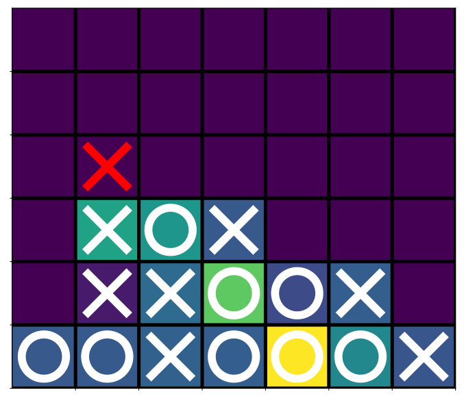
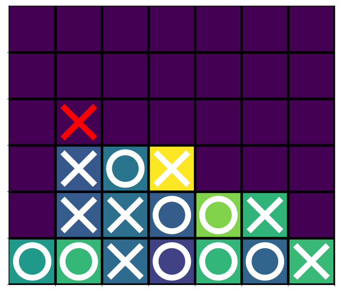
Figure 6: Top: One move explained by different saliency maps: The PI-50 agent placed a piece in the second column, blocking a potential win by their opponent (red cross). The saliency maps for this move are shown for each method. Bottom: The agent is presented with the colour information of the 50% most salient pieces according to each method (marked in white). This can lead to a different decision, here for LRP and Random, allowing the opponent to win.

We can now compare different saliency methods via the setup explained in Figure 1. As our agent we select PI-50 and allow to show 50% of colour features, thus remaining on-manifold. To implement the masker, we let an XAI-method explain the decision of the policy function for the most probable action. For every occupied field we sum the absolute value of saliency score from the first two colour channels (that represent which player occupies the field). The saliency scores on empty fields and on the third channel are ignored. Then we select the 50% (rounded up) highest scoring colour features and hide the rest from the board state (set them to 0). This state is then used by the player, (PI-50, non-competitive) to select a move. We present an illustration for all used saliency methods in Figure 6. Afterwards this process is mirrored by a different saliency method and this is iterated until the game is finished.

We compare the saliency methods Gradient, GuidedBackprop (GB) SmoothGrad, LRP- $\epsilon$ , DeepTaylor and Random from the Innvestigate⁸⁸ 8 https://github.com/albermax/innvestigate DBLP:journals/corr/abs-1808-04260 and DeepShap from the SHAP⁹⁹ 9 https://github.com/slundberg/shap toolboxes with recommended settings. Random, which assigns a random Gaussian noise as saliency value, Input, which shows the complete board state, and the FW-method explained in the previous chapter serve as comparison for the other methods.

We let each saliency method compete in a round-robin tournament with 1000 games for each encounter. In case of a draw, both methods score half a victory. We display the number of victories for each encounter in Figure 7 together with two challenges described in Section 4.3 and Section 3.3.

Results

The results are displayed in Figure 7. The methods form two groups of performance. DeepShap, GuidedBackprop and the Frank-Wolfe-based method perform best and equally well. The second group is formed by gradient, LRP and DeepTaylor who show a weaker performance. SmoothGrad has the worst showing, potentially owing to the fact that it does not automatically sample other valid board situations. These results are confirmed by the information-performance graphs, introduced in Section 3.3 for play against PI-50 with full information, where instead of randomly selecting the revealed features they are selected by each saliency method, see Figure 7.

Regarding FW, we showed in Section 4 that the optimiser does not always find what we consider the important pieces but rather the pieces that ensure the policy network makes the right decision. Thus DeepShap and GuidedBackprop compare very favourably considering FW optimises directly for winning the game. Additionally, DeepShap, Gradient, LRP- $\epsilon$ and GuidedBackprop severely outperform Shapley Sampling in finding the ground-truth pieces. This shows that heuristic methods can have merit over theoretically founded one. We explain a possible reason for the weak performance of the Shapley values and a way forward to improve it in Section 6.

Figure 7: Comparison of different XAI-methods playing Connect Four. Left: Win rates row vs column, with draws counting as

\frac{1}{2}

. Top right: Win rate of PI-50 with varying percentage of hidden information against itself. The partial colour features have been selected using the XAI-methods. The win rate of the agent decays slower, when the method is better at selecting the crucial information. Bottom right: Comparison of the XAI-methods in the ground truth task described in Section 4.3. We can see that DeepShap and GuidedBackprop perform well in all these tasks.

6 Conclusion

We have demonstrated that simple game setups can be used to train agents capable of handling missing features. This allowed us to design a proxy task for XAI-methods based on the idea that such agents make better decisions if provided more relevant information. We evaluate a collection of saliency methods and see strong performances for DeepShap and GuidedBackprop.

As explained in Section 2, using proxy tasks that evaluate the classifier off-manifold can have paradoxical consequence such as yielding “superstimulus” masks as the optimal strategy. To avoid this, we train our agents on the partial information used in our proxy task. Using the resulting characteristic function given by the policy network, we can directly calculate Shapley values via sampling. This attribution method is theoretically well understood and only relies inputs that were part of the training manifold which justifies trusting the resulting saliency maps.

However, one problem we discovered is that simply extending the training manifold is not enough if the training objective does not strongly regulate behaviour of the classifier. In our example the policy network is trained to predict sensible game actions—a task that becomes increasingly ill-defined for low information input. The additional entropy term was not strong enough to regulate behaviour towards a uniform distribution over all actions and thus the network output for many low information states was essentially random. A remedy could lie in using Q-learning instead, even in scenarios where it performs slightly worse than PPO as it only indirectly optimises for policy. Q-learning trains a value function to obey an consistency condition in form of the Bellman-equation Sutton and Barto, 2018. This indirectness can become useful since the objective remains well-defined even if almost no information is given. For a low average loss in terms of the Bellman equation the network would be required to give a conservative estimate of the board value, such as a 50% chance of winning. A similarly option for supervised learning on partial information is to include a default option of “I don’t know” that is preferred to a wrong answer. Then the objective on low information data becomes well defined and techniques such as Shapley sampling can be used as a theoretically sound saliency method. Tempering with the model to hide biases would require changing on-manifold behaviour which could be detected through performance tests.

In our investigation, the heuristic saliency methods compared very favourably to the more theoretically founded methods. The hope is that future research might prove guaranteed for time efficient methods, e.g. that DeepShap indeed provides a good approximation to the true Shapley values for networks trained on real-world data. If these saliency attribution methods can be made robust to manipulation, e.g. by approaches from Frye et al., 2020 and Anders et al., 2020, they could constitute promising tools for XAI.

Acknowledgements

This research was partially supported by the DFG Cluster of Excellence MATH+ (EXC-2046/1, project id 390685689) and the Research Campus Modal funded by the German Federal Ministry of Education and Research (fund numbers 05M14ZAM,05M20ZBM).

References

Adadi and Berrada, (2018) Adadi, A. and Berrada, M. (2018). Peeking inside the black-box: a survey on explainable artificial intelligence (xai). IEEE access, 6:52138–52160.
Adebayo et al., (2018) Adebayo, J., Gilmer, J., Muelly, M., Goodfellow, I., Hardt, M., and Kim, B. (2018). Sanity checks for saliency maps. arXiv preprint arXiv:1810.03292.
Allis, (1988) Allis, L. V. (1988). A knowledge-based approach of connect-four. J. Int. Comput. Games Assoc., 11(4):165.
Anders et al., (2020) Anders, C., Pasliev, P., Dombrowski, A.-K., Müller, K.-R., and Kessel, P. (2020). Fairwashing explanations with off-manifold detergent. In International Conference on Machine Learning, pages 314–323. PMLR.
Arrieta et al., (2020) Arrieta, A. B., Díaz-Rodríguez, N., Del Ser, J., Bennetot, A., Tabik, S., Barbado, A., García, S., Gil-López, S., Molina, D., Benjamins, R., et al. (2020). Explainable artificial intelligence (xai): Concepts, taxonomies, opportunities and challenges toward responsible ai. Information Fusion, 58:82–115.
Bach et al., (2015) Bach, S., Binder, A., Montavon, G., Klauschen, F., Müller, K.-R., and Samek, W. (2015). On pixel-wise explanations for non-linear classifier decisions by layer-wise relevance propagation. PLOS ONE, 10(7):1–46.
Biessmann and Refiano, (2021) Biessmann, F. and Refiano, D. (2021). Quality metrics for transparent machine learning with and without humans in the loop are not correlated. arXiv preprint arXiv:2107.02033.
Chalkiadakis et al., (2011) Chalkiadakis, G., Elkind, E., and Wooldridge, M. (2011). Computational aspects of cooperative game theory. Synthesis Lectures on Artificial Intelligence and Machine Learning, 5(6):1–168.
Clausen et al., (2021) Clausen, C., Reichhuber, S., Thomsen, I., and Tomforde, S. (2021). Improvements to increase the efficiency of the alphazero algorithm: A case study in the game’connect 4’. In ICAART (2), pages 803–811.
Crespo, (2019) Crespo, J. (2019). Reinforcement learning for two-player zero-sum games. Master’s thesis, Tecnico Lisboa, https://fenix.tecnico.ulisboa.pt/downloadFile/1689244997260153/81811-joao-crespo_dissertacao.pdf.
Dabas et al., (2022) Dabas, M., Dahiya, N., and Pushparaj, P. (2022). Solving connect 4 using artificial intelligence. In International Conference on Innovative Computing and Communications, pages 727–735. Springer.
Deng and Papadimitriou, (1994) Deng, X. and Papadimitriou, C. H. (1994). On the complexity of cooperative solution concepts. Mathematics of operations research, 19(2):257–266.
Dimanov et al., (2020) Dimanov, B., Bhatt, U., Jamnik, M., and Weller, A. (2020). You shouldn’t trust me: Learning models which conceal unfairness from multiple explanation methods. In SafeAI@ AAAI.
Dombrowski et al., (2019) Dombrowski, A.-K., Alber, M., Anders, C. J., Ackermann, M., Müller, K.-R., and Kessel, P. (2019). Explanations can be manipulated and geometry is to blame. arXiv preprint arXiv:1906.07983.
Doshi-Velez and Kim, (2017) Doshi-Velez, F. and Kim, B. (2017). Towards a rigorous science of interpretable machine learning. arXiv preprint arXiv:1702.08608.
Fong and Vedaldi, (2017) Fong, R. C. and Vedaldi, A. (2017). Interpretable explanations of black boxes by meaningful perturbation. In Proceedings of the IEEE international conference on computer vision, pages 3429–3437.
Frye et al., (2020) Frye, C., de Mijolla, D., Begley, T., Cowton, L., Stanley, M., and Feige, I. (2020). Shapley explainability on the data manifold. arXiv preprint arXiv:2006.01272.
Heo et al., (2019) Heo, J., Joo, S., and Moon, T. (2019). Fooling neural network interpretations via adversarial model manipulation. Advances in Neural Information Processing Systems, 32:2925–2936.
Hoeffding, (1994) Hoeffding, W. (1994). Probability inequalities for sums of bounded random variables. In The collected works of Wassily Hoeffding, pages 409–426. Springer.
Holzinger et al., (2017) Holzinger, A., Biemann, C., Pattichis, C. S., and Kell, D. B. (2017). What do we need to build explainable ai systems for the medical domain? arXiv preprint arXiv:1712.09923.
Huber et al., (2021) Huber, T., Limmer, B., and André, E. (2021). Benchmarking perturbation-based saliency maps for explaining deep reinforcement learning agents. arXiv preprint arXiv:2101.07312.
Jia et al., (2019) Jia, R., Dao, D., Wang, B., Hubis, F. A., Hynes, N., Gürel, N. M., Li, B., Zhang, C., Song, D., and Spanos, C. J. (2019). Towards efficient data valuation based on the shapley value. In The 22nd International Conference on Artificial Intelligence and Statistics, pages 1167–1176. PMLR.
Lapuschkin et al., (2019) Lapuschkin, S., Wäldchen, S., Binder, A., Montavon, G., Samek, W., and Müller, K.-R. (2019). Unmasking clever hans predictors and assessing what machines really learn. Nature communications, 10(1):1–8.
Li, (2017) Li, Y. (2017). Deep reinforcement learning: An overview. arXiv preprint arXiv:1701.07274.
Lipton, (2018) Lipton, Z. C. (2018). The mythos of model interpretability: In machine learning, the concept of interpretability is both important and slippery. Queue, 16(3):31–57.
(26) Lundberg, S. M. and Lee, S.-I. (2017a). A unified approach to interpreting model predictions. In Guyon, I., Luxburg, U. V., Bengio, S., Wallach, H., Fergus, R., Vishwanathan, S., and Garnett, R., editors, Advances in Neural Information Processing Systems 30, pages 4765–4774. Curran Associates, Inc.
(27) Lundberg, S. M. and Lee, S.-I. (2017b). A unified approach to interpreting model predictions. In Proceedings of the 31st international conference on neural information processing systems, pages 4768–4777.
Macdonald et al., (2021) Macdonald, J., Besançon, M., and Pokutta, S. (2021). Interpretable neural networks with frank-wolfe: Sparse relevance maps and relevance orderings. arXiv preprint arXiv:2110.08105.
Macdonald et al., (2019) Macdonald, J., Wäldchen, S., Hauch, S., and Kutyniok, G. (2019). A rate-distortion framework for explaining neural network decisions. arXiv preprint arXiv:1905.11092.
Macdonald et al., (2020) Macdonald, J., Wäldchen, S., Hauch, S., and Kutyniok, G. (2020). Explaining neural network decisions is hard. In XXAI Workshop, 37th ICML.
Mitchell et al., (2021) Mitchell, R., Cooper, J., Frank, E., and Holmes, G. (2021). Sampling permutations for shapley value estimation. arXiv preprint arXiv:2104.12199.
Mnih et al., (2015) Mnih, V., Kavukcuoglu, K., Silver, D., Rusu, A. A., Veness, J., Bellemare, M. G., Graves, A., Riedmiller, M., Fidjeland, A. K., Ostrovski, G., et al. (2015). Human-level control through deep reinforcement learning. nature, 518(7540):529–533.
Mohseni et al., (2021) Mohseni, S., Zarei, N., and Ragan, E. D. (2021). A multidisciplinary survey and framework for design and evaluation of explainable ai systems. ACM Transactions on Interactive Intelligent Systems (TiiS), 11(3-4):1–45.
Pokutta et al., (2020) Pokutta, S., Spiegel, C., and Zimmer, M. (2020). Deep neural network training with frank-wolfe. arXiv preprint arXiv:2010.07243.
Pons, (2019) Pons, P. (2019). Connect 4 game solver.
Ribeiro et al., (2016) Ribeiro, M. T., Singh, S., and Guestrin, C. (2016). " why should i trust you?" explaining the predictions of any classifier. In Proceedings of the 22nd ACM SIGKDD international conference on knowledge discovery and data mining, pages 1135–1144.
Ribeiro et al., (2018) Ribeiro, M. T., Singh, S., and Guestrin, C. (2018). Anchors: High-precision model-agnostic explanations. In Proceedings of the AAAI conference on artificial intelligence, volume 32.
Rudin, (2019) Rudin, C. (2019). Stop explaining black box machine learning models for high stakes decisions and use interpretable models instead. Nature Machine Intelligence, 1(5):206–215.
Rudin and Ustun, (2018) Rudin, C. and Ustun, B. (2018). Optimized scoring systems: Toward trust in machine learning for healthcare and criminal justice. Interfaces, 48(5):449–466.
Samek et al., (2017) Samek, W., Binder, A., Montavon, G., Lapuschkin, S., and Müller, K.-R. (2017). Evaluating the visualization of what a deep neural network has learned. IEEE Transactions on Neural Networks and Learning Systems, 28(11):2660–2673.
Schraagen et al., (2020) Schraagen, J. M., Elsasser, P., Fricke, H., Hof, M., and Ragalmuto, F. (2020). Trusting the x in xai: Effects of different types of explanations by a self-driving car on trust, explanation satisfaction and mental models. In Proceedings of the Human Factors and Ergonomics Society Annual Meeting, volume 64, pages 339–343. SAGE Publications Sage CA: Los Angeles, CA.
Schulman et al., (2017) Schulman, J., Wolski, F., Dhariwal, P., Radford, A., and Klimov, O. (2017). Proximal policy optimization algorithms. arXiv preprint arXiv:1707.06347.
Shapley, (2016) Shapley, L. S. (2016). 17. A value for n-person games. Princeton University Press.
Shih et al., (2018) Shih, A., Choi, A., and Darwiche, A. (2018). A symbolic approach to explaining bayesian network classifiers. arXiv preprint arXiv:1805.03364.
Shrikumar et al., (2017) Shrikumar, A., Greenside, P., and Kundaje, A. (2017). Learning important features through propagating activation differences. In International Conference on Machine Learning, pages 3145–3153. PMLR.
Silver et al., (2017) Silver, D., Schrittwieser, J., Simonyan, K., Antonoglou, I., Huang, A., Guez, A., Hubert, T., Baker, L., Lai, M., Bolton, A., et al. (2017). Mastering the game of go without human knowledge. nature, 550(7676):354–359.
Simonyan et al., (2013) Simonyan, K., Vedaldi, A., and Zisserman, A. (2013). Deep inside convolutional networks: Visualising image classification models and saliency maps. arXiv preprint arXiv:1312.6034.
Slack et al., (2020) Slack, D., Hilgard, S., Jia, E., Singh, S., and Lakkaraju, H. (2020). Fooling lime and shap: Adversarial attacks on post hoc explanation methods. In Proceedings of the AAAI/ACM Conference on AI, Ethics, and Society, pages 180–186.
Slack et al., (2021) Slack, D., Hilgard, S., Lakkaraju, H., and Singh, S. (2021). Counterfactual explanations can be manipulated. arXiv preprint arXiv:2106.02666.
Smilkov et al., (2017) Smilkov, D., Thorat, N., Kim, B., Viégas, F., and Wattenberg, M. (2017). Smoothgrad: removing noise by adding noise. arXiv preprint arXiv:1706.03825.
Springenberg et al., (2015) Springenberg, J. T., Dosovitskiy, A., Brox, T., and Riedmiller, M. A. (2015). Striving for simplicity: The all convolutional net. In ICLR (Workshop).
Sundararajan and Najmi, (2020) Sundararajan, M. and Najmi, A. (2020). The many shapley values for model explanation. In International Conference on Machine Learning, pages 9269–9278. PMLR.
Sutton and Barto, (2018) Sutton, R. S. and Barto, A. G. (2018). Reinforcement learning: An introduction. MIT press.
Vogt, (2019) Vogt, M. D. P. T. (2019). Carlo connect.
Wang et al., (2021) Wang, H., Preuss, M., and Plaat, A. (2021). Adaptive warm-start mcts in alphazero-like deep reinforcement learning. arXiv preprint arXiv:2105.06136.
Zeiler and Fergus, (2014) Zeiler, M. D. and Fergus, R. (2014). Visualizing and understanding convolutional networks. In Fleet, D., Pajdla, T., Schiele, B., and Tuytelaars, T., editors, Computer Vision – ECCV 2014, pages 818–833, Cham. Springer International Publishing.

Appendix A Saliency Methods and Off-Manifold Counterfactuals

Considering a classifier function $f:[0,1]^{d}\rightarrow[0,1]$ and an input $\mathbf{x}\in[0,1]^{d}$ , saliency methods attribute importance (or relevance) values to each input feature $x_{i}$ , with $i\in[d]$ , for the classifier decision $f(\mathbf{x})$ . In a sense they describe what the classifier focuses on. For a good introduction we refer to Adebayo et al., 2018. We now argue that the three categories of saliency methods introduced in Section 2 all rely on counter-factual inputs that lie off-manifold.