Virtual walks inspired by a mean field kinetic exchange model of opinion dynamics
Abstract
We propose two different schemes of realizing a virtual walk corresponding to a kinetic exchange model of opinion dynamics. The walks are either Markovian or non-Markovian in nature. The opinion dynamics model is characterized by a parameter which drives an order disorder transition at a critical value . The distribution of the displacements from the origin of the walkers is computed at different times. Below , two time scales associated with a crossover behavior in time are detected, which diverge in a power law manner at criticality with different exponent values. also carries the signature of the phase transition as it changes its form at . The walks show the features of a biased random walk below , and above , the walks are like unbiased random walks. The bias vanishes in a power law manner at and the width of the resulting Gaussian function shows a discontinuity. Some of the features of the walks are argued to be comparable to the critical quantities associated with the mean field Ising model, to which class the opinion dynamics model belongs. The results for the Markovian and non-Markovian walks are almost identical which is justified by considering the different fluxes. We compare the present results with some earlier similar studies.
Keywords:
Markov and non-Markovian processes, phase transitions, biased random walk, probability distribution, crossoverI Introduction
It is a common practice to study the dynamics of one physical system comprising of some interacting units by mapping it into another system of interacting particles or pseudo particles in a different space. Several such examples can already be found in the literature. The correspondence between the zero temperature spin coarsening dynamics in a Ising-Glauber model in one dimension privman; derrida1; derrida2; derri2 and the diffusive motion of the domain walls, which annihilate as they meet, is well known. In the voter model, one can conceive of a system of coalescing walkers which is equivalent to the dynamics of the agents liggett; krap; howard in any dimension. The dynamics of a opinion formation model in which the domain sizes play a key role, can also be studied by an equivalent system of annihilating walkers with a dynamic bias sbprps; reshmi.
On the other hand, one can directly represent the evolution of the state of a spin by the displacements of a virtual walker in the spin space. Such a walk picture has been recently used in pratik for a generalized Voter model and earlier, several aspects of this type of a walk have been considered in different systems dornic_g98; drouffe98; newman; balda; luck; drouffe2001, especially in the context of persistence behavior. In all these previous studies, one has a binary spin variable and the spin up (down) state at any time can be thought of as a displacement of the walker towards right (left) in the one dimensional space in that particular instant. In some of these works, the shape of the probability distribution of the displacements was shown to have some interesting features; in particular, it carries the signature of the phase transition, if any, occurring in the system.
Such virtual walks have been considered previously in systems other than spin or binary opinion dynamics models also. Here one may have more than two variables in the original system that can be mapped to a system of particles with binary states. For example, to study the stochastic properties, nucleotide sequences in a DNA was mapped onto a walk peng. For financial data, a random walk picture was introduced initially by Louis Bachelier bachelier. Later, similar walks were studied for models of wealth exchange econo1; econo2.
In this paper, we have considered a kinetic exchange model of opinion dynamics. Opinion dynamics models involving kinetic exchange type interactions have been studied in various ways during the last twenty years or so deffuant; toscani; lallouache; sb2011; ps2011; sociophysics. We have considered, in particular, the model proposed in soumya2012 and studied the version in which the opinions can have three discrete values. This model shows a phase transition driven by the disorder in the interaction between the agents. Several aspects of this model have been studied later sudip2016; ante2017; oester2019; sbsmps2020.
The mean field case, where any agent can interact with any other, has been considered here. We have studied two schemes for the walk, one of them is Markovian (Scheme I) process and the other non-Markovian (Scheme II). We show that the phase transition can be detected from the behavior of the distribution , where is the displacement of the walker at time , for both the walks. The walks show a crossover behavior in time in the ordered phase from which two time scales can be defined which diverge close to the critical point with different exponent values. We also find that an individual walker is like a biased random walker below the critical point while above it, the bias vanishes. The behavior of two particular features of the walks can be argued to be comparable to those of the order parameter and specific heat of the mean field Ising model.
In section II, we have described the opinion dynamics model under consideration and the related walks in detail. The results obtained are presented and analyzed in section III. In the last section, we summarize the work with some conclusive statements.
II Description of the opinion dynamics model and the virtual walks
We consider the kinetic exchange model (KEM) of opinion dynamics introduced in soumya2012. However, instead of continuous values, we take the case where the opinions can take three discrete values, 0 and . In this model, , the opinion of the th individual at time changes by a pair-wise interaction in the following manner
| (1) |
Here and the choice of pairs is unrestricted, i.e., this model is defined on a fully connected graph. is the interaction parameter representing the influence of the th agent on the th individual. It can take values ; a negative value is taken with probability , the only parameter in the model. The opinion value is bounded, if it becomes higher (lower) than then it is made equal to . In a system of agents, the quantity is defined as the order parameter. The above mean field model can be exactly solved yielding a order-disorder phase transition at , with Ising like criticalitysoumya2012.
We have associated a walker to each of the individuals of the system in a virtual one dimensional space. The position of the -th walker at time step in this space can be written as
At each step the walker can perform one of the three following actions: it can move to the nearest-neighbor site to its right or left or it can remain at its present location. So, is a random number which can take values ,, or . In this work, we consider the displacements to depend on the opinion states. We have used two schemes to implement the walk.
Scheme I is a Markovian process, i.e. here depends on the present opinion states only:
Scheme II is a non-Markovian walk where the depends on the present as well as the previous opinion states in the following way:
The values of thus chosen are tabulated in Table 1. In either case we take for all . It is to be emphasized here that the evolution of the opinions directly involves the parameter . The walks on the other hand are solely determined on the basis of the opinions in the last one or two steps and does not directly enter into the definition of the walk.
| Scheme I | Scheme II | ||
| 1 | 1 | 1 | 1 |
| 1 | 0 | 0 | -1 |
| 0 | 0 | 0 | 0 |
| 0 | 1 | 1 | 1 |
| 0 | -1 | -1 | -1 |
| -1 | 0 | 0 | 1 |
| -1 | -1 | -1 | -1 |
III Results


We have numerically simulated the kinetic exchange model of opinion dynamics on a fully connected graph of size and started with a completely random configuration, i.e., at , the number of individuals with opinions , and is taken to be for each. One Monte Carlo Step (MCS) consists of updates. In each update two different individuals are chosen randomly and the opinion of the first individual is updated according to eq. 1. The maximum system size simulated is and the maximum number of configurations over which averaging has been done is 2000. The time up to which the model is simulated depends on .
We first show the world lines of the walkers as is varied in Fig. 1. Each of these snapshots is taken for 20 individuals chosen randomly from a system with . It may be noted that for both the schemes, for small , at very early stages, the walk is centered around zero. At later stages, the walkers are more or less directed, either towards the left or right, with small diversions in the other direction which lasts for comparatively much shorter periods of time as shown in Figs 1a and b. However, for larger , observations over a longer timescale shows that there are occasional changes in the direction and the walker stays in the same direction over finite intervals of time (see Fig. 1c). As exceeds , there is a distinct change in the behavior of the trajectories, we find that walkers are more or less localized with no apparent bias (Fig. 1d). The picture at for larger times, rules out the possibility that the walk is entirely ballistic, as we see occasional directional changes, more so as increases as indicated in Fig. 1.
To gain more quantitative information, the probability distribution for the position of the walkers at time is estimated. The range of is .

Before discussing the nature of the distribution, we present the results for a crossover effect noted in time, for . During early times, shows a single peak at but at larger timescales one can observe a crossover from the centrally peaked distribution to a double peaked one. The positions of the two peaks are symmetric about the origin. The peaks of occur at larger values of (Fig. 2) as increases. To characterize this crossover behavior, we estimate the ratio where is the maximum value of . A study of the variation of with time shows that it remains close to unity till a time , then vanishes exponentially for . The results for a particular value of are shown in Fig. 3a. While is the timescale up to which the transient (single peaked) behavior of is observed, another timescale may be defined from the observation beyond . Fig. 3b shows the variation of the two timescales as a function of . As we approach the critical point , and both diverge as
| (2) |
We thus obtain two new critical exponents and ; for Scheme I and for Scheme II and is equal to for Scheme I and for Scheme II. We note that the exponent values differ by less than ten percent for the two schemes. The values of the exponents are also shown in Table 2.
For , shows a single peak at the origin and there is no crossover behavior in time. In Fig. 4, for different values at long times shows that the distribution becomes a single peaked one from a double peaked form at in both the schemes. Thus we see that the signature of the phase transition is indeed captured in the virtual walks.


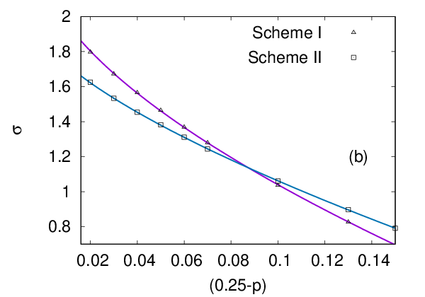
We next discuss the form of the distribution beyond the crossover time. As already mentioned, for there are two peaks occurring symmetrically on both sides of the origin. It is therefore sufficient to focus on, say, . It is natural to have as a first check whether a distribution for a walk is random (either biased or unbiased). We indeed find that a nice collapse can be obtained by plotting against where independent of and (for ) is a function of . The resulting collapsed curve is seen to fit to a Gaussian form, i.e., where the width depends on . For , we find a similar collapse with . In this regime, the Gaussian curve has a width which is nearly a constant except for very close to (which may be a finite size effect). All these results are presented in Fig. 5.
The above results show that the walks are like biased random walks for and like an unbiased walk above criticality. However, we note that we have here a biased walk where the bias can be positive and negative, i.e., will have both positive and negative values. It is expected that as , should vanish. This is indeed true and we note by analyzing the data that
| (3) |
As a function of , can be fitted in the following way:
| (4) | |||||
with indicating there is a discontinuity at . We will come back to this point later in the last section. The data for and are plotted in Fig. 6 for which the above forms have been obtained.
The qualitative behavior discussed above is again true for both the schemes but the values of the parameters differ for the two schemes. We observe that the walk for Scheme II takes place in a more zig-zag manner such that the net displacement is larger for Scheme I. The precise values of the parameters occurring in eqs 3 and 4 are given in Table 2.
| Scheme I | |||||||
|---|---|---|---|---|---|---|---|
| Scheme II |


We try to justify next why the two schemes give almost identical results for the exponents , and . ( is different for the two walks but it is actually not a critical exponent). The fact is, as Table 1 shows, the difference in the two schemes occurs only when the opinion state changes from a non-zero value to zero. Note that below , as the order parameter is non-zero, we expect an excess of either opinion value 1 or -1. For a configuration where, say, opinion dominates, the expression for the fractions of opinion values can be obtained from soumya2012 below as
| (5) |
where . Hence the flux of states with nonzero opinion to zero opinion will be equal to and where
| (6) |
The values of these fluxes are in general less than that of the other fluxes, for example, is given by
| (7) |
The first term in eq.7 arises due to the interaction with an agent with opinion value zero, which occurs with probability . In Fig. 7, the above three fluxes are shown for comparison that indicates that transition to states with zero values are rarer such that the dynamics in Scheme I and Scheme II may become nearly identical.

IV Summary and discussions
In this work, we have considered one dimensional walks in a virtual space corresponding to a kinetic exchange model of opinion dynamics. Two different schemes have been conceived, one Markovian and the other non-Markovian. The expected feature that the walks contain the signature of the phase transition is obtained. This was also found in pratik.
A crossover behavior in time is also observed and the results show the existence of two timescales which diverge close to the known critical point with two new exponents. It has been checked that this crossover behavior does not vanish in the thermodynamic limit. Such a crossover was also noted in the voter model pratik, although the distribution showed a different form.
The form of the distribution function shows that the individual walkers perform biased random walk motion where the bias is either to the left or right in the ordered phase. Such a distribution is not noted for similar walks corresponding to binary spin models like the Ising model or generalized voter models in two dimensions. For these models, the displacement of the walker was taken to be simply equal to the spin state. Although Scheme I is a similar walk, in the present case, since one has a spin zero state as well, the walks are not equivalent which gives rise to the difference in the nature of . Above the critical point of course, one has a Gaussian walk when the displacements become uncorrelated, independent of the particular model.
We would also like to add that here we get a biased walk where the bias can be positive and negative with equal probability on an average. Hence, if one considers the entire distribution, one will get for all . This will give for and for . Note that in ordinary biased random walk, in contrast. Using either the region or we obtained as in the biased random walk. We argue it is better to regard the distribution to the left and right of the origin separately, consistent with the snapshots which clearly reveal the biased nature of the walks below . We also find that the bias goes to zero above and is therefore analogous to an order parameter. Indeed, the critical exponent associated with is very close to 0.5, the known value for , the order parameter in the opinion dynamics model (or Ising model) in the mean field case.
We also observed a discontinuity in the value of at . In fact the behavior of is quite similar to that of the specific heat of the mean field Ising model with the critical exponent equal to zero and a jump discontinuity stanley. Note that both and specific heat are measures of fluctuation. So we claim that from these walks, not only the transition point can be detected, one can also obtain an estimate of the static critical points.
As far as the present two schemes are concerned, one gets nearly identical exponents for the time scales which diverge and the bias that vanishes close to the critical point. A brief analysis helps us to understand why this is so. However, the motion of the walkers is more zig-zag in Scheme II, that leads to a reduced bias and the width of the distribution shows different results quantitatively in the two schemes as a result. In principle, the walks can be conceived in many other ways, so although three exponents show comparable values, one cannot immediately conclude that a universal behavior exists for all virtual walks. Still, it is interesting that the Markovian and the non-Markovian walks show similar behavior.
Authors’ Contributions
The work has been formulated and the manuscript prepared by both authors. Simulations were carried out by SS.
Funding
Research by SS is supported by the Council of Scientific and Industrial Research, Government of India through CSIR NET fellowship (CSIR JRF Sanction No. 09/028(1134)/2019-EMR-I). PS has received support from SERB (Government of India) scheme no MAT/2020/000356.
References
- (1) Privman V. 1997 Nonequilibrium Statistical Mechanics in One Dimension (Cambridge University Press, Cambridge).
- (2) Derrida B, Bray AJ and Godrèche C. 1994 Non-trivial exponents in the zero temperature dynamics of the 1D Ising and Potts models J. Phys. A 27, L357.
- (3) Derrida B. 1995 Exponents appearing in the zero-temperature dynamics of the 1D Potts model. J. Phys. A Math. Theor. 28, 1481.
- (4) Derrida B, Hakim V, Pasquier V. 1995 Exact First-Passage Exponents of 1D Domain Growth: Relation to a Reaction-Diffusion Model. Phys. Rev. Lett. 75, 751.
- (5) Liggett TM. 1985 Interacting Particle Systems (Springer, New York).
- (6) Krapivsky PL, Redner S, Ben-Naim E. 2010 A Kinetic View of Statistical Physics. (Cambridge University Press, Cambridge).
- (7) Howard M and Godrèche C. 1998 Persistence in the Voter model: continuum reaction-diffusion approach. J. Phys. A 31, L209.
- (8) Biswas S, Ray P, Sen P. 2011 Opinion dynamics model with domain size dependent dynamics: novel features and new universality class. Journal of Physics : Conference Series, 297, 012003.
- (9) Roy R, Ray P, Sen P. 2020 Tagged particle dynamics in one dimensional models with the particles biased to diffuse towards their nearest neighbour. J. Phys. A: Math. Theor. 53, 155002.
- (10) Mullick P and Sen P. 2018 Virtual walks in spin space: A study in a family of two-parameter models. Phys. Rev. E 97, 052122.
- (11) Dornic I and Godrèche C. 1998 Mathematical and General Large deviations and nontrivial exponents in coarsening systems . J. Phys. A 31 5413.
- (12) Drouffe JM and Godrèche C. 1998 Journal of Physics A: Mathematical and General Stationary definition of persistence for finite-temperature phase ordering . J. Phys. A 31, 9801.
- (13) Newman TJ and Toroczkai Z. 1998 Diffusive persistence and the ”sign-time” distribution. Phys. Rev. E 58, R2685.
- (14) Baldassarri A, Bouchaud JP, Dornic I and Godrèche C. 1999 Statistics of persistent events: An exactly soluble model . Phys. Rev. E 59, R20.
- (15) Godrèche C and Luck JM. 2001 Statistics of the Occupation Time of Renewal Processes. J. Stat. Phys. 104, 489.
- (16) Drouffe JM and Godrèche C. 2001 Temporal correlations and persistence in the kinetic Ising model: the role of temperature Eur. Phys. J. B 20, 281.
- (17) Peng CK. 1992 Long-range correlations in nucleotide sequences. Nature 356, 168.
- (18) Bachelier L. 1900 Theorie de la speculation, Annales Scientifiques de I’Ecole Normale Superiure, 3 (17), pp. 21-86.
- (19) Chatterjee A and Sen P. 2010 Agent dynamics in kinetic models of wealth exchange. Phys. Rev. E 82, 056117.
- (20) Goswami S, Chatterjee A and Sen P. 2011 Antipersistent dynamics in kinetic models of wealth exchange. Phys. Rev. E 84, 051118.
- (21) Deffuant G, Neau D, Amblard F, Weisbuch G. 2000 Mixing beliefs among interacting agents. Advances in Complex Systems, 3, 87.
- (22) Toscani G. 2006 Kinetic models of opinion formation. Communications in Math- ematical Sciences,4, 481.
- (23) Lallouache M, Chakrabarti A.S, Chakraborti A, and Chakrabarti B.K. 2010 Opinion formation in kinetic exchange models: Spontaneous symmetry-breaking transition. Phys. Rev. E, 82,056112.
- (24) Sen P. 2011 Phase transitions in a two-parameter model of opinion dynamics with random kinetic exchanges. Phys. Rev. E 83, 016108.
- (25) Biswas S. 2011 Mean-field solutions of kinetic-exchange opinion models. Phys. Rev. E 84, 056106.
- (26) Sen P, Chakrabarti BK. 2014 B.K.Sociophysics: An Introduction(Oxford University Press, Oxford) and the references therein.
- (27) Biswas S, Chatterjee A, Sen P. 2012 Disorder induced phase transition in kinetic models of opinion dynamics. Physica A 391, 3257.
- (28) Mukherjee S, Chatterjee A. 2016 Disorder-induced phase transition in an opinion dynamics model: Results in two and three dimensions. Phys. Rev. E 94, 062317.
- (29) Anteneodo C, Crokidakis N. 2017 Symmetry breaking by heating in a continuous opinion model. Phys. Rev. E 95, 042308.
- (30) Oestereich AL, Pires MA, Crokidakis N. 2019 Three-state opinion dynamics in modular networks. Phys. Rev. E 100, 032312.
- (31) Mukherjee S, Biswas S, Sen P. 2020 Long route to consensus: Two-stage coarsening in a binary choice voting model. Phys. Rev. E 102, 012316.
- (32) Stanley HE. 1971 Introduction to Phase Transitions and Critical Phenomena(Oxford University Press, London).