Hybrid Mechanical and Electronic Beam Steering for Maximizing OAM Channel CapacityThanks: This work was supported in part by the Natural Science Basic Research Program of Shaanxi under Grant 2021JZ-18 and in part by the Natural Science Foundation of Guangdong Province of China under Grant 2021A1515010812 and in part by the open research fund of National Mobile Communications Research Laboratory, Southeast University under Grant 2021D04.Thanks: R. Chen is with the State Key Laboratory of ISN, Xidian University, Xi’an 710071, China, and also with the National Mobile Communications Research Laboratory, Southeast University, Nanjing 210018, China (e-mail: rchen@xidian.edu.cn).Thanks: Z. Tian and W.-X. Long are with the State Key Laboratory of Integrated Service Networks (ISN), Xidian University, Shaanxi 710071, China.Thanks: X. Wang is with the Electrical Engineering Department, Columbia University, New York, NY 10027 USA (e-mail: wangx@ee.columbia.edu).Thanks: W. Zhang is with the School of Electrical Engineering and Telecommunications, The University of New South Wales, Australia, (e-mail: w.zhang@unsw.edu.au).
Abstract
Radio frequency-orbital angular momentum (RF-OAM) is a novel approach of multiplexing a set of orthogonal modes on the same frequency channel to achieve high spectrum efficiencies. Since OAM requires precise alignment of the transmit and the receive antennas, the electronic beam steering approach has been proposed for the uniform circular array (UCA)-based OAM communication system to circumvent large performance degradation induced by small antenna misalignment in practical environment. However, in the case of large-angle misalignment, the OAM channel capacity can not be effectively compensated only by the electronic beam steering. To solve this problem, we propose a hybrid mechanical and electronic beam steering scheme, in which mechanical rotating devices controlled by pulse width modulation (PWM) signals as the execution unit are utilized to eliminate the large misalignment angle, while electronic beam steering is in charge of the remaining small misalignment angle caused by perturbations. Furthermore, due to the interferometry, the receive signal-to-noise ratios (SNRs) are not uniform at the elements of the receive UCA. Therefore, a rotatable UCA structure is proposed for the OAM receiver to maximize the channel capacity, in which the simulated annealing algorithm is adopted to obtain the optimal rotation angle at first, then the servo system performs mechanical rotation, at last the electronic beam steering is adjusted accordingly. Both mathematical analysis and simulation results validate that the proposed hybrid mechanical and electronic beam steering scheme can effectively eliminate the effect of diverse misalignment errors of any practical OAM channel and maximize the OAM channel capacity.
Index Terms:
Orbital angular momentum (OAM), uniform circular array (UCA), hybrid mechanical and electronic, beam steering.I Introduction
The rapid development of emerging applications, such as high-definition (HD) video, virtual reality (VR) and auto-pilot driving, results in a never-ending growth in mobile data traffic. It is recognized that the next 6G communication system will be required to increase the capacity of current 5G systems hundred fold [1]. To meet the requirement, more and more high frequency bands such as millimeter wave and terahertz bands are being licensed. As radio frequency (RF) spectrum resources are scarce, besides exploiting more frequency bandwidth, innovative techniques to enhance spectrum efficiency (SE) have been explored, such as advanced coding, cognitive radio (CR) and ultra-massive multiple-input multiple-output (MIMO). In essence, all these techniques are based on planar electromagnetic (EM) waves physically.
Since the discovery in 1992 that light beams with helical phase fronts can carry orbital angular momentum (OAM) [2], a significant research effort has also been focused on vortex EM waves as a novel approach to carrying a set of orthogonal OAM modes on the same frequency channel and achieving high-SE mode multiplexing[3, 4, 5, 6, 7, 8, 9, 10, 11, 12, 13, 14, 15, 16, 17]. Multiple OAM modes could significantly reduce the receivers complexity, compared to a MIMO single mode communication, without affecting the system capacity[6, 16]. The helical phase wave front of vortex EM is described by a phase term , where is the transverse azimuthal angle and is an infinite integer, known as topological charge or OAM mode number [2]. So far, there have been several methods to generate radio OAM beams such as using spiral phase plate (SPP) [4], solid cylinder dielectric resonator antenna [18], tri-mode concentric circularly polarized patch antenna, metallic traveling-wave ring-slot structure [19], time-switched array structure [20], uniform circular array (UCA) [21, 8, 11] and metasurface [22], among which UCA is the most popular device because of the ubiquitous application of antenna array on 4G, 5G and even 6G base stations (BSs) and its compatibility with MIMO beam steering[11]. Therefore, we focus on the UCA rather than other particular antenna structures for OAM waves’ generation and reception in this paper.
Since OAM communication requires precise alignment of the transmit and the receive antennas, the electronic beam steering approach has been proposed for the uniform circular array (UCA)-based OAM communication system to circumvent large performance degradation induced by small antenna misalignment in practical environments [7, 11]. However, in large-angle misalignment case, the OAM channel capacity can not be effectively compensated only by the electronic beam steering, which has not been investigated before as far as we know. Moreover, it is observed that when multiple OAM modes are transmitted simultaneously, due to the interferometry, the electric field intensities of the multi-mode OAM beam are not uniform on the ring of its main lobe. Hence, the receive signal-to-noise ratios (SNRs) are not equal at the elements of the receive UCA, which results in the OAM channel capacities being quite different at different rotation angles of the receive UCA around its axis.

In this paper, to deal with the aforementioned problems, we first propose a hybrid mechanical and electronic beam steerable transceiver structure, which consists of a UCA fixed with mechanical rotation devices in pitch, roll and yaw directions, respectively, as shown in Fig. 1. Specifically, the coarse alignment is first achieved by mechanical beam steering, and then electronic beam steering is exploited to compensate the small-scale misalignment error caused by perturbations, such as random wind, rain, or installation errors [23]. The principle of electronic beam steering for UCA-based OAM communication system is compensating the changed phases caused by oblique angle at the transmit or receive UCA through adjusting the delays of antenna elements by phase shifters, then the normal phases used only for OAM piralization/despiralization are tuned to the new phases used for both OAM piralization/despiralization and beam steering towards the direction of departure/arrival of OAM beams [7]. Furthermore, due to the interferometry, the receive UCA needs rotating to an optimal angle for maximizing the OAM channel capacity. The mathematical analysis and numerical simulations show that the proposed hybrid mechanical and electronic beam steering scheme outperforms the traditional scheme of only using electronic beam steering, especially in the practical case of large misalignment error, and obtaining the maximum OAM channel capacity. The novelty and major contributions of this paper are summarized as follows:
- •
First, based on the line-of-sight (LoS) OAM channel model, we show mathematically why only using electronic beam steering is not enough for compensating the performance degradation of OAM channel capacity in the large-angle misalignment case.
- •
Second, we propose the hybrid mechanical and electronic beam steering scheme to effectively improve the OAM channel capacity in practical environments, in which mechanical rotating devices controlled by pulse width modulation (PWM) signals as the execution unit are utilized to eliminate the large misalignment angle, while electronic beam steering is in charge of the remaining small misalignment angle caused by perturbations.
- •
Third, considering that the rotation angle of the receive UCA around its axis has a large effect on the receive signal-to-noise ratio (SNR) due to the interferometry, we propose a rotatable UCA structure for the OAM receiver to maximize the channel capacity, for which the simulated annealing algorithm is adopted to obtain the optimal rotation angle at first, then the servo system performs mechanical rotation, at last the electronic beam steering is adjusted accordingly.
The remainder of this paper is organized as follows. In Section II, we model the UCA-based LoS OAM communication system with hybrid mechanical and electronic beam steerable transceiver. In Section III, the effect of electronic beam steering in large-angle misalignment case is analyzed. In Section IV, to deal with the performance degradation of electronic beam steering in large-angle misalignment case and maximize the OAM channel capacity, we propose the hybrid mechanical and electronic beam steering scheme. Simulation results are shown in Section V and conclusions are summarized in Section VI.
Notations: Bold lowercase letters denote column vectors, and bold uppercase letters denote matrices. and denote transpose and conjugate transpose. is identity matrix. and denote the Hadamard product and modulus. represents expectation.

| (1) |
II UCA-Based OAM Communication Systems
In this paper, we focus on a UCA-based line-of-sight (LoS) OAM communication system as considered in [6, 8, 7, 10, 11, 23, 12, 24]. Since the transmit UCA and the receive UCA need to be aligned, beam steering approach is proposed to achieve beam alignment between the UCAs at both sides [7, 11]. As the functions of the transmit beam steering and the receive beam steering are the same, in order to evaluate the effects of mechanical beam steering and electronic beam steering, we have to separate the effects of transmit and receive beam steering and only consider one side. Therefore, we assume the transmit UCA having been aligned to the center of the receive UCA through mechanical rotation, while the receive UCA will align to the transmit UCA through yaw and pitch mechanical rotations firstly, and then electronic beam steering more accurately in real time, as shown in Fig. 1. Thus, this geometric model falls into the non-parallel misalignment case [7, 11], as shown in Fig. 2.
In the considered OAM communication system, a multi-mode OAM beam is generated by an -element UCA at the transmitter and received by another -element UCA at the receiver. For higher data rate transmission, orthogonal frequency-division multiplexing (OFDM)-based LoS multi-carrier and multi-mode OAM (MCMM-OAM) communication scheme proposed in [11, 12] is adopted, and we assume subcarriers and OAM modes for data transmission, subcarriers and OAM modes for coarse angle of arrival (AoA) estimation, and subcarriers and OAM modes for refined AoA estimation.
II-A Channel Model
The geometrical model of the UCA-based LoS OAM channel is illustrated in Fig. 2. In this model, the transmitter coordinate system is established using the transmit UCA plane as the XOY plane and the axis through the transmit UCA center O and perpendicular to the transmit UCA plane as the Z-axis, and the receiver coordinate system is established on the plane of the receive UCA by the similar approach, where -axis and -axis correspond to the pitch axis and the roll axis in Fig. 1, respectively. Since the transmit UCA is aligned with the center of the receive UCA in the non-parallel misalignment case, the spherical coordinate of the receive UCA center can be denoted as in in the non-parallel misalignment case. Suppose the point D is the projection of the point O on the plane, and the spherical coordinate of the transmit UCA center is denoted as in , where is the distance between the transmit and the receive UCA centers, is the azimuth angle, is the elevation angle, and and are defined as the AoA of the OAM beam[11, 12].
The coordinate system is built so that its origin is at the point O and plane is parallel to . Meanwhile, we build the coordinate system so that its origin is at the point and plane is parallel to XOY, where -axis corresponds to the yaw axis in Fig. 1. According to the geometrical model, the angle between -axis and Z-axis is , so is that between -axis and -axis. Denote the angle between the -axis and the -axis as (), so is that between X-axis and -axis, where . Denote the angle between the -axis and the -axis as (), so is that between Y-axis and -axis, where , and could be obtained as , and can be obtained by the OAM AoA estimation method[11, 12]. The proof of is given in Appendix A. Then, could be calculated as (1), whose proof is given in Appendix B. Denote the angle between the line and X-axis as and the angle between the line and -axis as , where is the position of the th () element at the transmitter, is the position of the th () element at the receiver, and , and are respectively the corresponding initial angles of the first reference antenna elements in both UCAs.
According to Fig. 2, the cartesian coordinate of the th antenna element on the transmit UCA is in coordinate system, and the cartesian coordinate of the th antenna element on the receive UCA can be written as in coordinate system, where and are respectively the radii of the transmit and receive UCAs. In order to calculate the distance between the th antenna element on the transmit UCA and the th antenna element on the receive UCA, we transform the coordinate of the th antenna element on the receive UCA in coordinate system to the coordinate in coordinate system. Hence, the cartesian coordinate of the th antenna element on the receive UCA in coordinate system, denoted by , can be obtained as [25], where and representing the axis rotation matrixes corresponding to the pitch direction and yaw direction, respectively, take the forms
| (2) |
Thus, the cartesian coordinate of the th antenna element on the receive UCA in coordinate system can be written as[17]
| (3) |
As the coordinate system is parallel to , the cartesian coordinate of the th antenna element of the receive UCA in coordinate system, denoted by , can be obtained as . With the above coordinates, we can obtain the transmission distance from the th transmit antenna element to the th receive antenna element. By assuming that the transmit and receive UCAs are in far-field distance region of each other, thus and , we can approximate as
| (4) |
where (a) uses the method of completing a square and the condition as same as the simple case , (b) is directly obtained from the condition of . In LoS communications, propagation through the RF channel leads to attenuation and phase rotation of the transmitted signal. This effect is modelled through multiplying by a complex constant , whose value depends on the frequency and the distance between the transmit and receive antennas, as
| (5) |
where , (a) neglects a few minor terms in the denominator of the amplitude term and thus only is left, is the wave number at the th subcarrier, and is the wavelength at the th subcarrier, and denotes the degradation of amplitude, , models all the constants relative to each receive antenna element, and the complex exponential term is the phase difference due to the propagation distance. In order to mainly analyze the factors we concerned, the transmission loss caused by the polarization mismatch between the transmit and receive UCAs is ignored.
Then, the channel matrix of the UCA-based LoS communication system can be expressed as . Note that when and , is a circulant matrix that can be decomposed by the -dimentional Fourier matrix as , where is a diagonal matrix with the eigenvalues of on its diagonal. In [6, 7, 8, 11], the OAM channel is defined as , which will become in perfect alignment case.
II-B Signal Model
As a UCA can generate multi-mode OAM beams with the baseband (partial) discrete Fourier transform (DFT) matrix , the equivalent baseband signal models of transmitting multi-mode OAM data symbols could be expressed as , where is used for spiralization, contains the modulation symbols transmitted on OAM modes at the th subcarrier simultaneously, is the th OAM mode number. Thus, the received OAM signal can be written as
| (6) |
where is a right circularly shifted (partial) Fourier matrix used for despiralization, , is the complex Gaussian noise vector with zero mean and covariance matrix , , , is the received information signal on the th mode OAM and the th subcarrier of receiver, and can be written as
| (7) |
is the th-row and th-column element of , and can be expressed as
| (8) |
, , and . In (7), carries useful signals. Once or , , which becomes interferences.
For this model, in order to alleviate the interference that is resulted by the large misalignment error in the practical case, we propose the hybrid mechanical and electronic beam steering scheme, as shown in Fig. 1. It can be observed from (II-A) that mechanical rotations of the UCA plane will result in the changes of , and the amplitudes and phases of . It is worth noting that the amplitude and phase of do not linearly change with the rotation angles, which are dependent on , and . Therefore, the mechanical beam steering is a non-linear transformation for the channel matrix . In order to represent the operation of the mechanical beam steering, we assume a non-linear function and then the effect of mechanical beam steering on the channel matrix can be expressed as
| (9) |
where is the estimate of by the OAM AoA estimation technique, is the estimate of obtained with and the estimate of , i.e., , and is the optimal value of the rotation angle in roll direction for maximizing the OAM channel capacity, so , and are mechanical rotation angles in the pitch, yaw and roll directions, respectively, and is the channel matrix after mechanical rotations of the receive UCA. In contrast to the mechanical beam steering, the electronic beam steering is linear transformation [7, 11]. With the hybrid non-linear mechanical beam steering and linear electronic beam steering, the recovered information signal vector becomes
| (10) |
where is the electronic beam steering matrix at the receiver. The procedure of the mechanical and electronic beam steering for the LoS OAM communication receiver will be detailed in Section IV.
III The Effect of Electronic Beam Steering and Solution in Large-Angle Misalignment Case
The motivation of the proposed hybrid beam steering is from practical implementation of mmWave relays. Let us consider the case in the Fig. 3(a), no matter it is OAM array or mmWave massive MIMO array, the performance of the communication is poor. However, with the proposed the hybrid beam steering scheme, which first enables the coarse alignment between the transmit array plane and the receive array plane through mechanical rotation as in Fig. 3(b), the good performance can be expected through refined electronic beam steering.

III-A The Effect of Electronic Beam Steering
In this section, we first investigate the effect of electronic beam steering, especially in large-angle misalignment case. With only electronic beam steering, the recovered information signal vector takes the form [11]
| (11) |
where is defined as the effective OAM channel matrix after electronic beam steering, the electronic beam steering matrix of the receive UCA is designed as , and , , , , , is the information symbol on the th mode OAM and the th subcarrier after electronic beam steering, and can be written as
| (12) |
is the th-row and th-column element of , and can be expressed as
| (13) |

Hence, after electronic beam steering, the signal-to-interference-plus-noise ratio (SINR) on the th mode and the th subcarrier can be formulated as
| (14) |
where is the average power of modulation symbols on the th mode and th subcarrier. We assume that the average power of modulation symbols on all modes and subcarriers are the same, and then the SINR approaches to the signal-to-interference ratio (SIR) at high SNR as
| (15) |
where . Then, we evaluate how the SINRs change with the increase of and of the electronic beam steering. If we substitute (13) into (III-A), the obtained two-dimensional function of and is too complex to analyze. Therefore, we turn to check how changes with the increase of when , and how changes with the increase of when , and obtain the following results.
Proposition 1.
When , the SIR after electronic beam steering on the th mode and th subcarrier decreases with the increase of as goes to zero.
Proof:
The proof is given in Appendix C. ∎
Proposition 2.
When , the SIR after electronic beam steering on the th mode and th subcarrier decreases with the increase of as goes to zero.
Proof:
The proof is completely similar to Proposition 1. ∎
The Proposition 1 and Proposition 2 show that is monotonically decreasing for and in two one-dimensional directions respectively on the condition that approaches to zero. Moreover, we show through simulation results in Fig. 4(a) and Fig. 4(b) that is also monotonically decreasing for and in the case is larger. Furthermore, Fig. 4(c) shows that when is fixed to be a value other than zero, is still monotonically decreasing for and . It follows that with the increase of oblique angles the SINR after applying only electronic beam steering will get worse.
In order to further figure out the total effect of all the subcarriers, the MCMM-OAM system with only electronic beam steering can be evaluated according to the channel capacity
| (16) |
In Fig. 5, we illustrate what is the condition for “small-angle misalignment” so that electronic steering is sufficient, and what is the condition for “large-angle misalignment” so that it is insufficient. It can be seen apparently from the figure that under this set of parameters the threshhold between “small-angle” and “large-angle” is about 20 degree. When and are smaller than the threshold, the electronic beam steering can well compensate for the performance loss caused by misalignment, while and are larger than this threshold, the electronic beam steering is not good enough especially when and approach .
| (18) |
III-B Solution in Large-Angle Misalignment Case
The reason for the performance degradation of electronic beam steering is that with the increase of misalignment angles, the inter-mode interferences increase. In order to minimize the value of the interference term , we observe from (13) that the smaller the and , the smaller the value of the interference term. As long as the and are equal to zero, and interferences disappear. It follows that when the receive UCA is in the large-angle misalignment with the transmit UCA, it is the best choice to firstly steer the yaw and pitch directions of the receive UCA physically in order that and are as small as possible. Furthermore, besides minimizing the interference, maximizing the channel capacity needs also maximizing the received signal power, that is, maximizing the term . Note that when and are fixed, for the receive UCA only has effect on , which means the roll rotation angle needs to be optimized. The above analysis could be formulated in the follows.
| (17) |
This is the motivation of proposing hybrid mechanical and electronic beam steering. Mechanical beam steering enables the misalignment angles fall into the range of “small angle” and leave them for electronic beam steering, which happens when the receiver starts running or moves to another place.
IV Hybrid Mechanical and Electronic Beam Steering of OAM Communication Systems
According to (III-B), the procedure of the hybrid mechanical and electronic beam steering scheme can be designed as the four successive steps shown in Fig. 6. Then, the hybrid beam steering can be formulated as (III-A), where is the recovered information signal vector with hybrid beam steering, is defined as the effective OAM channel matrix after the hybrid steering, , is the first electronic beam steering matrix in pitch and yaw directions, is the second beam steering matrix that represents adjusting the electronic beam in roll direction, represents the operation of the first mechanical beam steering in pitch and yaw directions, and represents the operation of the second mechanical beam steering in roll direction.
The implementation of mechanical beam steering relies on the servo system of mechanical rotating devices, which is controlled by PWM signals [26]. The schematic diagram of the servo system corresponding to the hybrid OAM transceiver in Fig. 1 is shown in Fig. 7, where the control unit generates three tunable PWM signals for pitch-axis, yaw-axis and roll-axis, respectively. In the execution unit, intelligent power modules (IPMs) are used to drive steering gears in the three directions respectively, and potentiometer is used to convert the motion of steering gear to voltage and feedback to control unit. We denote the accuracy of the potentiometer as . The relationship between the duty cycle of the PWM signal and the expected rotation angle can be obtained as , where is the signal period of PWM signal, , and are the pulse widths of PWM signal corresponding to the minimum angle, middle angle and the maximum angle of the mechanical rotating device [27]. Here, represents , and in pitch-axis, yaw-axis and roll-axis, respectively.
IV-A Mechanical Beam Steering in Pitch and Yaw Directions
Firstly, the coarse alignment is achieved by mechanical beam steering. From the Fig. 1 we can see that only with rotations in pitch and yaw directions can the receive UCA align to the transmit UCA. Then, according to the Fig. 2, we can see that the mechanical beam steering in yaw and pitch directions are performed around -axis and -axis, respectively. It is assumed that and are the coarse estimates of and in this step, and and are the remaining small misalignment errors in yaw and pitch directions, respectively. In the first-stage yaw direction, the mechanical beam steering makes the receive UCA rotate around the -axis of the coordinate system so that the angle between the -axis and the -axis changes from to . Then, in the second-stage pitch direction, the receive UCA rotates around the rotated -axis so that the angle between the -axis and -axis changes from to . With the pitch and yaw rotations, the cartesian coordinate of the th antenna element on the receive UCA in , denoted by , can be obtained as , where and represent the coordinate rotation matrixes in pitch and yaw directions and considering the second-stage pitch rotation around the rotated -axis not any axis of the coordinate system, the axis rotation matrix is required after the first-stage yaw rotation for the coordinate transformation from -axis to -axis, in the end, performs the opposite coordinate transformation from -axis to -axis. Thus, after the pitch and yaw rotations the transmission distance from the th transmit antenna element to the th receive antenna element becomes
| (19) |
Hence, the channel matrix after the mechanical beam steering in pitch and yaw directions can be expressed as , where the th-row th-column element can be written as
| (20) |
(a) neglects a few small terms in the denominator and only is left. If only with the mechanical beam steering, the received OAM signal takes the form
| (21) |
where is defined as the effective multi-mode OAM channel matrix after the first mechanical beam steering. is the th-row and th-column element of , and can be calculated as
| (22) |
where , (a) applies the approximation for and in the case that and are relatively small, and neglects a few small terms under the condition . As is a non-diagonal matrix, we can conclude that there is still inter-mode interferences after the first mechanical beam steering.
IV-B Electronic Beam Steering in Pitch and Yaw Directions
In order to eliminate the inter-mode interferences induced by the remaining small perturbations and after previous mechanical beam steering, periodic refined AoA estimation are necessary. It is assumed that and varies slower than the duration of AoA estimation, and and can be perfectly estimated. With the estimates of and , electronic beam steering can enable the receive beam to align with the direction of the arrived OAM beam. The electronic beam steering matrix can be designed as , where and , , . After involving these phases into the original phases in at the receive UCA, the effective multi-mode OAM channel matrix at the th subcarrier becomes
| (23) |
Denote as the th-row and th-column element of , which can be expressed as
| (24) |
. Note that in (24), we have
That is to say, the non-diagonal elements of equal to zero approximately. It follows that after the mechanical and electronic beam steering in pitch and yaw directions, the inter-mode interferences are almost completely eliminated in the case of large-angle misalignment. At the same time, according to the conclusion in Section III, steering the OAM beam with only a small angle in electronic way does not result in large performance degradation. Therefore, the proposed hybrid mechanical and electronic beam steering outperforms only using electronic beam steering in a wide variety of practical scenarios.


IV-C Mechanical Rotation in Roll Direction for OAM Channel Capacity Maximization
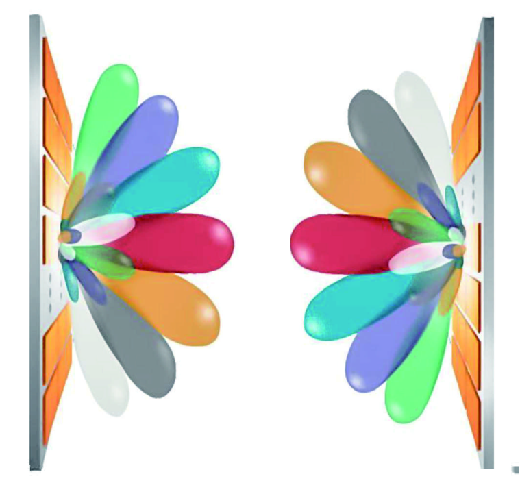
When a multi-mode OAM beam that can be deemed as the superposition of multiple OAM modes is transmitted, we can observe the phenomenon of interferometry as shown in the simulation results of HFSS in Fig. 8, that is, the electric field intensities of one multi-mode OAM beam are not uniform on the ring of its main lobe. Therefore, the receive antenna elements need to be set in the maximum SNR positions on the ring of the main lobe, which means that another rotation angle in roll direction within the plane of the receive UCA should be optimized. In order to obtain the optimal rotation angle in roll direction, we first formulate the optimization problem and then apply SA algorithm to solve the problem.
Input:
, , ,
Output:
IV-C1 Optimization Model
First, we denote the effective OAM channel matrix with twice mechanical and once electronic beam steering as . Since the roll rotation will result in the misalignment between the transmit and receive beams and deteriorate the performance of the OAM communication systems, we assume the second-step roll rotation can be well compensated by the forth-step electronic beam steering. Only in this way, can the effective OAM channel capacity be maximized. For this purpose, we denote the effective OAM channel matrix with twice mechanical and twice electronic beam steering as . Then, based on (24) the th diagonal element of can be obtained as
| (27) |
where is the rotation angle in roll direction. Therefore, the SINR at the th mode and th subcarrier can be formulated as . The channel capacity of the OAM communication system with hybrid beam steering can be expressed as
| (28) |
In order to see the impact of on OAM channel capacity intuitively, we plot the relationship between and in Fig. 9. It can be seen from the figure that the OAM channel capacity varies periodically with in the range of . That is because the antenna elements on the receive UCA are uniformly arranged around the center of the circle. In Fig. 9, leads to 10 cycles. Therefore, we can limit to only any circle of the range to obtain the optimal rotation angle from the following optimization problem.
Since the target function is not guaranteed to be differentiable, gradient-based procedures cannot be applied. A large number of global optimization techniques were developed to provide alternative solution methods for challenging problems, e.g., simulated annealing (SA) [28]. SA algorithm is a derivative-free promising algorithm, whose final solution quality does not strongly depend on the choice of the initial solution [29]. So, SA is adopted here to obtain the optimal rotation angle within the range . The solving procedure of the problem (IV-C1) is given in Algorithm 1, where is the initial temperature, is the lowest temperature, is the cooling coefficient, is the number of inner-layer iterations, is used to identify whether a new value is accepted at , is the optimal channel capacity, represents the new solution obtained in the algorithm, and represents the roll angle corresponding to . In the end, the optimal rotation angle that maximizes the OAM channel capacity can be obtained.
Remark 1.
We can observe from (27) and (IV-C1) that is only decided by {, , , }. That is to say, the mechanical beam steering in roll direction does not dependent on the electronic beam steering in pitch and yaw directions. Therefore, the procedure of hybrid mechanical and electronic beam steering can change its order from , , , to , , , . Thus, we have , which unifies (10) and (III-A). Therefore, the relationship between , and is .
IV-C2 Mechanical Rotation in Roll Direction
Having the optimal rotation angle , the servo system make the receive UCA rotate around the roll-axis. Since the mechanical beam steering in roll direction is just for maximizing the OAM channel capacity rather than aligning the transmit and receive beams, we don’t consider the rotation error in for easier analysis. According to the Fig. 2, the cartesian coordinate of the th antenna element on the receive UCA in coordinate system after the mechanical rotation in roll direction, denoted by , can be expressed as , where represents the coordinate rotation matrix in roll direction and can be expressed as
Thus, the cartesian coordinate of the th antenna element on the receive UCA in coordinate system, denoted by , can be expressed as , where and represent the axis rotation matrixes corresponding to the pitch direction and the yaw direction after the mechanical rotation in roll direction, respectively.
Hence, after roll rotation the transmission distance from the th transmit antenna element to the th receive antenna element can be calculated as
| (34) |
where . Correspondingly, the channel matrix can be expressed as , where the th-row th-column element can be written as
| (35) |
(a) neglects a few small terms in the denominator and thus only is left. Thus, the effective multi-mode OAM channel matrix after the roll rotation can be written as
| (36) |
where is the th-row and th-column element of , and can be calculated as
| (37) |
(a) applies the approximation for and in the case that and are relatively small, and neglects a few small terms under the condition .
IV-D Adjusting Electronic Beam in Three Directions
It can be seen from (37) that the effective multi-mode OAM channel matrix after roll rotation is not a diagonal matrix any more, because the transmit and receive beam directions are not aligned after the roll rotation. In order to solve the reemerging inter-mode interferences, the electronic beam has to be adjusted in pitch, yaw and roll directions. The beam adjustment matrix could be designed as , where and has the form
| (38) |
. After involving these phases into the original phases in at the receive UCA, the effective multi-mode OAM channel matrix at the th subcarrier becomes
| (39) |
Proposition 3.
The successive implementation of the electronic beam steering matrices and can eliminate the inter-mode interferences in the channel matrix after mechanical beam steering .
Proof:
Successive implementing and to leads to the th-row and th-column element of being expressed as
| (40) |
where (a) applies the approximation for and in the case that, and are relatively small, and neglects a few small terms under the condition . According to (IV-B), it is apparent that the th diagonal element of can be expressed as
| (41) |
and the non-diagonal elements of approximately equal to zero. It follows that the successive implementation of the electronic beam steering matrices and can eliminate the inter-mode interferences. ∎
Remark 2.
According to the Proposition 3, the procedure of the hybrid mechanical and electronic beam steering for the LoS MCMM-OAM receiver can be simplified from the four steps , , , illustrated in Fig. 6 to only the two steps: mechanical beam steering in pitch, yaw and roll directions and electronic beam steering in pitch, yaw and roll directions .
IV-E Complexity Analysis
The specific computational complexity of the proposed hybrid mechanical and electronic beam steering scheme is compared with that of traditional electronic beam steering in the Table I. For LoS MCMM-OAM communication systems, whether the coarse distance and AoA estimation method or the refined distance and AoA estimation method, their complexities are both determined by the complexity of the EVD in (16) of reference [11]. However, the complexity of the coarse distance and AoA estimation method is affected by the values of and , and factors that affect the complexity of the refined distance and AoA estimation method are the values of and . Moreover, the complexity of the electronic beam steering is determined by the complexity of the multiplying the received signal vector by . It follows that the values of , and decide the complexity of the electronic beam steering. The complexity of is determined by the complexity of the mechanical rotation in pitch and yaw directions, and the value of , and decide the complexity of the . Meanwhile, the complexity of the is determined by the complexity of the mechanical rotation in roll direction corresponding to the value of and . The complexity of the optimization algorithm is determined by the values of , , and . The total computational complexity comparison between the hybrid mechanical and electronic beam steering and electronic beam steering scheme is shown in the Fig. 10. It can be seen from the Fig. 10 that due to the coarse AoA estimation using fewer OAM modes and subcarriers, mechanical beam steering and optimization having relatively low complexity, the total complexity of the proposed hybrid beam steering scheme is only slightly higher than that of traditional electronic beam steering. Furthermore, we calculate the relative complexity from the proposed hybrid beam steering to electronic beam steering as . To show their difference, we select parameters as , , , , , , , , , , , , and . With these parameters, the complexity of the hybrid beam steering is 1.009 to 1.026 times that of the electronic beam steering.
| Scheme | Complexity | |
| Hybrid BS | Coarse AoA estimation | |
| Mechanical beam steering | ||
| Optimization algorithm | ||
| Mechanical beam steering | ||
| Refined AoA estimation | ||
| Electronic beam steering | ||
| Electronic BS | AoA estimation | |
| Electronic beam steering | ||
V Numerical Simulations And Results
In this section we show the performance of the proposed hybrid mechanical and electronic beam steering method by numerical simulations. We first verify the effectiveness of SA algorithm in solving the optimal solution , and show the convergence rate of the algorithm. Then, we compare the channel capacities of the UCA-based LoS MCMM-OAM system with the proposed hybrid beam steering and that with only electronic beam steering. Unless otherwise stated, the SNRs in all the figures are defined as the ratio of the received signal power versus the noise power. In the simulations, we choose subcarriers from GHz to GHz, , , with , , , , , , , .
Fig.11 shows the solution of the optimization problem (IV-C1). It can be seen from the figure that the channel capacity with obtained rotation angle by Algorithm 1 reaches its optimum. In Fig.12, we show the convergence rate of the Algorithm 1 with the number of outer-layer iterations, where , and . It can be clearly seen that through reasonably setting the parameters of SA algorithm, the target function has a fast convergence rate.
In Fig.13, we illustrate the channel capacities of the proposed hybrid mechanical and electronic beam steering scheme and the channel capacities of only using electronic beam steering method under different pitch, yaw and roll rotation angles. Also, the channel capacities in the case of perfect alignment is given for clearer comparison. It can be seen from the results that for the electronic beam steering method, the larger the oblique angles, the lower the channel capacity, while the proposed hybrid mechanical and electronic beam steering scheme can effectively eliminate the effect of large misalignment errors of any practical OAM channel and approaches the performance of perfect aligned OAM channel.
Although we performed simulations at 4GHz, the proposed hybrid mechanical and electronic beam steering scheme is applicable to all frequency bands due to that the channel capacity in (28) is dependent on the two terms and related to frequency in (27). Recall that , and , we set , and to be different times of in the simulations. As the difference of and is so small within a certain bandwidth that the values of and do not vary much with frequency. The simulation results in higher frequencies used in 5G and 6G are similar to those at 4GHz, which are omitted here due to limited space.
VI Conclusions
In this paper, a hybrid mechanical and electronic beam steering scheme is proposed for LoS multi-carrier and multi-mode OAM communication systems to deal with the capacity loss encountered by electronic beam steering in large misalignment condition. To intuitively reveal the motivation of the proposed hybrid beam steering scheme, we show from both mathematical proof and numerical simulations that only using the electronic beam steering method, the larger the oblique angles, the lower the receive SINR and OAM channel capacity. In our proposed hybrid beam steering scheme, mechanical rotating devices controlled by PWM signals are utilized to eliminate the large misalignment angle, while electronic beam steering is in charge of the remaining small misalignment angle caused by perturbations. The whole procedure is designed as four consecutive steps including mechanical beam steering in pitch and yaw directions, electronic beam steering in pitch and yaw directions, mechanical rotation in roll direction and adjusting electronic beam in pitch, yaw and roll directions. As the physical beam steering in mechanical way is nonlinear operation for channel matrix, while electronic beam steering in digital way is linear operation, we show that the four steps of hybrid beam steering can be simplified to only two steps, i.e., mechanical beam steering in pitch, yaw and roll directions and electronic beam steering in these three directions. Numerical simulations show that searching for the optimal roll rotation angle only requires no more than 30 iterations with the SA algorithm, and the proposed hybrid beam steering scheme can effectively eliminate the effect of large misalignment errors of any practical OAM channel approaching the performance of perfect aligned OAM channel.
It is worth noting that for the OAM communication system in the large off-axis and more general misalignment cases, the proposed hybrid mechanical and electronic beam steering scheme is still applicable with the same idea in [7] that beam steering is performed at both receiver and transmitter. However, the specific procedure needs to be further developed, which can also be used in mmWave massive MIMO systems. Moreover, the directivity of the antenna units will affect the rotation angle . Although in this manuscript the antenna elements are assumed to be ideally omnidirectional, we believe that it is of practical significance to study how the directivity of the antenna units affect the rotation angle , which is left for our future work.

| (B.3) |
In order to prove the relationship between , and , we illustrate the geometrical relationship between , and in Fig. A1. We assume that A is the point on the -axis with its cartesian coordinate in the coordinate system , is the point that A rotates around -axis the angel to. Thus, the cartesian coordinate of is . is the point that rotates around -axis the angel to. Thus, the cartesian coordinate of is . Therefore, the distance between A and can be obtained as
| (A.1) |
According to the law of cosines, . Thus, can be expressed as
| (A.2) |
Because the cartesian coordinate of the point in the coordinate system can be easily obtained as , is on the -axis. Therefore, the angle between -axis and Z-axis is . Hence, the relationship between the , and can be obtained as .
In order to prove (1), we first magnify the geometrical model of the receive UCA of Fig. 2 when as Fig. B1(a). In the coordinate system , the cartesian coordinates of the point and O are and , respectively. We assume that B is the point on the -axis, is the point on the -axis, and their cartesian coordinates in the coordinate system are and , respectively. So, the cartesian coordinates of B and are and in the coordinate system , respectively. With the cartesian coordinates of , and B, we can obtain the plane equation of the receive UCA , where , , , and . Thus, the distance from the point O to the plane of receive UCA can be written as
| (B.1) |
With the cartesian coordinates of B and O, the distance between O and B can be obtained as
| (B.2) |
Since the line OD is perpendicular to the plane of the receive UCA, it is perpendicular to the line DB. Hence, OD, DB and OB form a right triangle, where OD and DB are two legs and OB is hypotenuse. Therefore, the distance from D to B can be expressed as (B.3). With the cartesian coordinates of and B, we can calculate as
| (B.4) |


Similarly, the line OD is perpendicular to due to OD being perpendicular to the plane of the receive UCA. Hence, OD, and form a right triangle, where OD and are two legs and is hypotenuse. Hence, can be written as
| (B.5) |
According to the law of cosines, . Therefore,
| (B.6) |
Since B is on the -axis while is on the -axis, . Meanwhile, and , Therefore, can be obtained as when .
Similarly, when , the geometrical model of the receive UCA is shown in Fig. B1(b). We can prove in the same way that when .
On one hand, when and , the th diagonal element of can be obtained as
| (C.1) |
where is defined as
| (C.2) |
When goes to zero, . Therefore, can be approximated as
| (C.3) |
According to [11], we can substitute the Taylor series expansion of the exponential function into (C.3) and eventually have , where .
| (C.6) |
On the other hand, when and , the th-row and th-column element of can be obtained as
| (C.4) |
where is defined as
| (C.5) |
We substitute into and obtain (C.6). For the last summation in (C.6), it is easy to verify that
| (C.7) |
When , we always have (recall that ) according to (34) of [11]. When , (C.7) is always zero, i.e., the Taylor series of does not contain the terms , and when , (C.7) equals to if and only if ; . Furthermore, when , the coefficient of is much smaller due to the term , and hence the term is counted into the higher order infinitesimal of denoted as as goes to zero. Thus, (C.5) can be approximated as
| (C.8) |
where . Therefore, (C.4) can be approximated as
| (C.9) |
Then, similar to the approximation of the summation term with Taylor series expansion in (C.3), (C.9) can be further approximated as
| (C.10) |
where .
In order to analyze how changes with the increase of when , we first express the reciprocal of when as
| (C.11) |
It is obvious that (C.11) consists of three terms and the derivative of (C.11) is the sum of their derivatives. Moreover, the derivative of is given as
| (C.12) |
where
| (C.13) |
| (C.14) |
| (C.15) |
and .
When , , thus the sign of the derivative of depends on and . We can find that when , and , thus can be written as
| (C.16) |
Because , . Hence, the derivative of is greater than zero so that is increasing with ; when , and , thus can be written as
| (C.17) |
It can be seen from (C.17) that . Therefore, the derivatives of every term of are greater than zero so that the term is increasing with ; when , and . We can find that when , can be expressed as
| (C.18) |
when , can be expressed as
| (C.19) |
Thus, when , . Therefore, the derivatives of every term of are greater than zero so that is increasing with .
When , the reciprocal of can be written as
| (C.20) |
It is obvious that (C.20) consists of two terms and the derivative of (C.20) is the sum of their derivatives. Moreover, when , . When or , and , thus
| (C.21) |
Hence, the derivatives of every term of and are greater than zero so that and are increasing with .
Therefore, we get the conclusion that is decreasing with when . On the contrary, we can prove in the same way that is increasing with when . Overall, the Proposition 1 that is decreasing with is proved.
References
- [1] H. Tataria, M. Shafi, A. F. Molisch, M. Dohler, H. SjÖland, and F. Tufvesson, “6G wireless systems: Vision, requirements, challenges, insights, and opportunities,” Proc. IEEE, vol. 109, no. 7, pp. 1166–1199, 2021.
- [2] L. Allen, M. W. Beijersbergen, R. J. C. Spreeuw, and J. P. Woerdman, “Orbital angular momentum of light and the transformation of Laguerre-Gaussian laser modes,” Phys. Rev. A, Gen. Phys., vol. 45, no. 11, pp. 8185–8189, Jun. 1992.
- [3] F. Tamburini, E. Mari, A. Sponselli, B. Thidé, A. Bianchini, and F. Romanato, “Encoding many channels on the same frequency through radio vorticity: First experimental test,” New J. Phys., vol. 14, no. 3, p. 033001, 2012.
- [4] Y. Yan et al., “High-capacity millimetre-wave communications with orbital angular momentum multiplexing,” Nature Commun., vol. 5, no. 1, p. 4876, Dec. 2014.
- [5] Y. Ren et al., “Line-of-sight millimeter-wave communications using orbital angular momentum multiplexing combined with conventional spatial multiplexing,” IEEE Trans. Wireless Commun., vol. 16, no. 5, pp. 3151–3161, May 2017.
- [6] W. Zhang, S. Zheng, X. Hui, R. Dong, X. Jin, H. Chi, and X. Zhang, “Mode division multiplexing communication using microwave orbital angular momentum: An experimental study,” IEEE Trans. Wireless Commun., vol. 16, no. 2, pp. 1308–1318, Feb. 2017.
- [7] R. Chen, H. Xu, M. Moretti, and J. Li, “Beam steering for the misalignment in UCA-based OAM communication systems,” IEEE Wireless Commun. Lett., vol. 7, no. 4, pp. 582–585, Aug. 2018.
- [8] R. Chen, W. Yang, H. Xu, and J. Li, “A 2-D FFT-based transceiver architecture for OAM-OFDM systems with UCA antennas,” IEEE Trans. Veh. Technol., vol. 67, no. 6, pp. 5481–5485, Jun. 2018.
- [9] C. Zhang and Y. Zhao, “Orbital angular momentum nondegenerate index mapping for long distance transmission,” IEEE Trans. Wireless Commun., vol. 18, no. 11, pp. 5027–5036, Nov. 2019.
- [10] R. Chen, H. Zhou, M. Moretti, X. Wang, and J. Li, “Orbital angular momentum waves: Generation, detection and emerging applications,” IEEE Commun. Surveys Tuts., vol. 22, no. 2, pp. 840–868, 2nd Quart., 2020.
- [11] R. Chen, W.-X. Long, X. Wang, and J. Li, “Multi-mode OAM radio waves: Generation, angle of arrival estimation and reception with UCAs,” IEEE Trans. Wireless Commun., vol. 19, no. 10, pp. 6932–6947, Oct. 2020.
- [12] W.-X. Long, R. Chen, M. Moretti, and J. Li, “AoA estimation for OAM communication systems with mode-frequency multi-time ESPRIT method,” IEEE Trans. Veh. Technol., vol. 99, no. 1, Apr. 2021.
- [13] W.-X. Long, R. Chen, M. Moretti, J. Xiong, and J. Li, “Joint spatial division and coaxial multiplexing for downlink multi-user OAM wireless backhaul,” IEEE Trans. Broadcasting, vol. 67, no. 4, pp. 1–15, Dec. 2021.
- [14] X. Zhang et al., Orbital Angular Momentum Based Structured Radio Beams and its Applications. John Wiley & Sons, Ltd, 2021, ch. 9, pp. 269–293.
- [15] X. Xiong, S. Zheng, Z. Zhu, X. Yu, X. Jin, and X. Zhang, “Performance analysis of plane spiral OAM mode-group based MIMO system,” IEEE Commun. Lett., vol. 24, no. 7, pp. 1414–1418, 2020.
- [16] A. Trichili, K.-H. Park, M. Zghal, B. S. Ooi, and M.-S. Alouini, “Communicating using spatial mode multiplexing: Potentials, challenges, and perspectives,” IEEE Commun. Surveys Tuts., vol. 21, no. 4, pp. 3175–3203, 2019.
- [17] Z. Tian, R. Chen, W.-X. Long, H. Zhou, and M. Moretti, “Broadband beam steering for misaligned multi-mode OAM communication systems,” J. Syst. Eng. Electron., vol. 32, no. 4, pp. 779–788, Aug. 2021.
- [18] J. Liang and S. Zhang, “Orbital angular momentum (OAM) generation by cylinder dielectric resonator antenna for future wireless communications,” IEEE Access, vol. 4, pp. 9570–9574, Apr. 2016.
- [19] W. Zhang, S. Zheng, X. Hui, Y. Chen, X. Jin, H. Chi, and X. Zhang, “Four-OAM-mode antenna with traveling-wave ring-slot structure,” IEEE Antennas Wireless Propag. Lett., vol. 16, pp. 194–197, 2017.
- [20] A. Tennant and B. Allen, “Generation of radio frequency OAM radiation modes using circular time-switched and phased array antennas,” in Proc. Loughborough Antennas Propag. Conf. (LAPC), Nov. 2012, pp. 1–4.
- [21] S. M. Mohammadi, L. K. S. Daldorff, J. E. S. Bergman, R. L. Karlsson, B. Thide, K. Forozesh, T. D. Carozzi, and B. Isham, “Orbital angular momentum in radio A system study,” IEEE Trans. Antennas Propag., vol. 58, no. 2, pp. 565–572, Feb. 2010.
- [22] Y. Shen, J. Yang, H. Meng, W. Dou, and S. Hu, “Generating millimeter-wave Bessel beam with orbital angular momentum using reflective-type metasurface inherently integrated with source,” Appl. Phys. Lett., vol. 112, no. 14, p. 141901, Apr. 2018.
- [23] M. Jian, Y. Chen, and G. Yu, “Non-coaxial OAM: Precoding design, misaligned parameter estimation and capacity compensation,” IEEE Access, vol. 9, pp. 37 726–37 738, 2021.
- [24] Y. Yagi, H. Sasaki, T. Yamada, and D. Lee, “200 Gb/s wireless transmission using dual-polarized OAM-MIMO multiplexing with uniform circular array on 28 GHz band,” IEEE Antennas and Wireless Propag. Lett., vol. 20, no. 5, pp. 833–837, 2021.
- [25] Y. Rahmat-Samii, “Useful coordinate transformations for antenna applications,” IEEE Trans. Antennas Propagat., vol. 27, no. 4, pp. 571–574, 1979.
- [26] M. F. N. Tajuddin, N. H. Ghazali, M. F. Mohammed, B. Ismail, Z. M. Isa, T. C. Siong, and N. Ghazali, “TMS320F2812 digital signal processor (DSP) implementation of DPWM,” in Proc. IEEE Student Conf. Res. Develop. (SCOReD), 2009, pp. 142–145.
- [27] N. Pinckney, “Pulse-width modulation for microcontroller servo control,” IEEE Potentials, vol. 25, no. 1, pp. 27–29, 2006.
- [28] S. Xavier-de Souza, J. A. K. Suykens, J. Vandewalle, and D. Bolle, “Coupled simulated annealing,” IEEE Trans. Syst. Man Cybern. B, vol. 40, no. 2, pp. 320–335, 2010.
- [29] M. Abido, “Robust design of multimachine power system stabilizers using simulated annealing,” IEEE Trans. Energy conversion, vol. 15, no. 3, pp. 297–304, 2000.
![[Uncaptioned image]](2202.11693v2/RuiC.png) |
Rui Chen (S’08-M’11) received the B.S., M.S. and Ph.D. degrees in Communications and Information Systems from Xidian University, Xi’an, China, in 2005, 2007 and 2011, respectively. From 2014 to 2015, he was a visiting scholar at Columbia University in the City of New York. He is currently an associate professor and Ph.D. supervisor in the school of Telecommunications Engineering at Xidian University. He has published more than 80 papers in international journals and conferences and held 40 patents. He is an Associate Editor for International Journal of Electronics, Communications, and Measurement Engineering (IGI Global). His research interests include broadband wireless communication systems, array signal processing and intelligent transportation systems. |
![[Uncaptioned image]](2202.11693v2/ZhenyangT.png) |
Zhenyang Tian (S’18) received the B.S. degree in Electronical Information Science and Technology from the Shanxi University, Taiyuan, China, in 2020. He is currently pursuing the M.S. degree in communications and information systems with Xidian University. His research interests include orbital angular momentum (OAM) communication systems and array signal processing. |
![[Uncaptioned image]](2202.11693v2/WenxuanL.png) |
Wen-Xuan Long (S’18) received the B.S. degree (with Highest Hons.) in Rail Transit Signal and Control from Dalian Jiaotong University, Dalian, China in 2017. She is currently pursuing a double Ph.D. degree in Communications and Information Systems at Xidian University, China and University of Pisa, Italy. Her research interests include broadband wireless communication systems and array signal processing. |
![[Uncaptioned image]](2202.11693v2/XW.png) |
Xiaodong Wang (S’98-M’98-SM’04-F’08) received the Ph.D. degree in electrical engineering from Princeton University. He is currently a Professor of electrical engineering with Columbia University, New York, NY, USA. He has authored the book Wireless Communication Systems: Advanced Techniques for Signal Reception (Prentice-Hall, 2003). His research interests include computing, signal processing, and communications, and has published extensively in these areas. His current research interests include wireless communications, statistical signal processing, and genomic signal processing. He was a recipient of the 1999 NSF CAREER Award, the 2001 IEEE Communications Society and Information Theory Society Joint Paper Award, and the 2011 IEEE Communication Society Award for Outstanding Paper on New Communication Topics. He was an Associate Editor for the IEEE TRANSACTIONS ON COMMUNICATIONS, the IEEE TRANSACTIONS ON WIRELESS COMMUNICATIONS, the IEEE TRANSACTIONS ON SIGNAL PROCESSING, and the IEEE TRANSACTIONS ON INFORMATION THEORY. He is listed as an ISI highly cited author. |
![[Uncaptioned image]](2202.11693v2/WeiZ.png) |
Wei Zhang (S’01-M’06-SM’11-F’15) received the Ph.D. degree in Electronic Engineering from the Chinese University of Hong Kong in 2005. Currently, he is Professor at School of Electrical Engineering and Telecommunications, the University of New South Wales, Sydney, Australia. His research interests include space information networks, IoT, and massive MIMO. He has published over 200 papers and holds 5 US patents. He received 5 best paper awards from international conferences, IEEE Communications Society (ComSoc) TCCN Publication Award, and ComSoc Asia Pacific Outstanding Paper Award. He was ComSoc Distinguished Lecturer in 2016-2017 and the Editor-in-Chief of IEEE Wireless Communications Letters in 2016-2019. Currently, he serves as Area Editor of IEEE Transactions on Wireless Communications and Editor-in-Chief of Journal of Communications and Information Networks. He also serves in Steering Committee of IEEE Networking Letters and IEEE Transactions on Green Communications and Networking. He is Chair for IEEE Wireless Communications Technical Committee and Vice Director of the IEEE ComSoc Asia Pacific Board. He was a member of Fellow Evaluation Committee of IEEE Vehicular Technology Society in 2016-2019. He served on the organizing committee of the IEEE ICASSP 2016 and the IEEE GLOBECOM 2017. He was TPC Chair of APCC 2017 and ICCC 2019. He is a member of ComSoc IT Committee, TC Recertification Committee, and Finance Standing Committee. He is Member-at-Large of ComSoc in 2018-2020. |