跳到论文正文
W Papers独立论文阅读器 arXiv:2202.11685 论文正文 计算阅读时间 · 0%
引用这篇论文根据当前论文元数据生成,正式投稿前建议核对。


License: CC BY 4.0
arXiv:2202.11685v1 [cs.LG] 23 Feb 2022
 

A Class of Geometric Structures in Transfer Learning:
Minimax Bounds and Optimality


Xuhui Zhang          Jose Blanchet          Soumyadip Ghosh          Mark S. Squillante

Stanford University          Stanford University          IBM Research          IBM Research

Abstract

We study the problem of transfer learning, observing that previous efforts to understand its information-theoretic limits do not fully exploit the geometric structure of the source and target domains. In contrast, our study first illustrates the benefits of incorporating a natural geometric structure within a linear regression model, which corresponds to the generalized eigenvalue problem formed by the Gram matrices of both domains. We next establish a finite-sample minimax lower bound, propose a refined model interpolation estimator that enjoys a matching upper bound, and then extend our framework to multiple source domains and generalized linear models. Surprisingly, as long as information is available on the distance between the source and target parameters, negative-transfer does not occur. Simulation studies show that our proposed interpolation estimator outperforms state-of-the-art transfer learning methods in both moderate- and high-dimensional settings.

1 INTRODUCTION

The task of transferring knowledge from one domain (source) to another related domain (target) is known as transfer learning. This task arises naturally in a wide range of applications where data is scarce in the target domain but substantial in a source domain believed to be somewhat similar to the target. For example, in the context of marketing and demand prediction for products in a new market, it is natural to use source information involving well-tested markets. Similarly, demand prediction for new products can be estimated using source information from current market products (Afrin et al. 2018). Rigorous statistical formulations of transfer learning introduce non-trivial challenges. This includes balancing the tension between tractability in the training procedure and flexibility in order to reflect the differences between the source and target environments. In addition to this tension, a useful modeling framework should provide statistical insights on the efficiency gain induced by introducing source information into target inference.

Our goal in this paper is to introduce a transfer learning formulation under linear and generalized linear models that addresses the above tractability-flexibility tension and produces effective efficiency insights. In particular, the contributions of this paper include:

(ii) Our formulation provides an easy-to-compute transfer learning estimator that optimally (in a precise sense) interpolates the target and source parameters subject to an uncertainty region which controls the differences between source and target models.

(i​iii) Our modelling framework exposes a natural geometric structure that is built on using the Fisher information metric (also known as information geometry) which we exploit in order to understand the main drivers of transfer learning from source to target.

(i​i​iiii) We are able to provide a finite-sample minimax lower bound and show that the worst-case risk of our estimator in (ii) achieves (up to a constant) the minimax lower bound uniformly over the magnitude of the difference between the target and source models.

One of the insights from our formulation, for example, is that as long as information is available on the distance between the source and target parameters, negative-transfer does not occur. Namely, the worst-case risk of our estimator in (ii) is always smaller than the minimax risk of using the target dataset alone.

Although there is a significant amount of literature on applied transfer learning procedures (Pan and Yang 2009; Torrey and Shavlik 2010; Weiss et al. 2016; Taskesen et al. 2021), the literature on rigorous mathematical formulations that lead to minimax optimal estimators is limited. Cai and Wei 2021 consider transfer learning in the context of a stylized non-parametric classification setting under a different set of assumptions including a model that only allows posterior drift. Kpotufe and Martinet 2021 study classification settings similar to that of Cai and Wei 2021, albeit under covariate-shift assumptions on the difference in source and target environments. In strong contrast, while our methodology is parametric, our analysis is not limited to classification problems and it further supports more general environments including more general drift conditions between the target and source models, where indeed our analysis of the underlying geometry explicitly accounts for these differences.

Bastani 2021 considers linear and non-linear regression models similar to our work, and proposes a two-step joint estimator for transfer learning. However, their focus is on high-dimensional settings under sparsity assumptions and no minimax optimality result is established; moreover, since they use an l1l_{1} norm for the analysis, their results are not directly comparable to our results. Li et al. 2020 extend the work of Bastani 2021 to allow multiple source domains and establish a minimax lower bound for high-dimensional linear regression models (LRMs). However, their bound is asymptotic in the number of target samples, and they further constrain the difference between the source and target parameters relative to the size of the target sample.  Tian and Feng 2021 further extend this work of Li et al. 2020 to high-dimensional generalized linear models (GLMs). In strong contrast, we study a fixed-difference environment without any such constraint and the performance of our optimal estimator is measured in terms of finite-sample bounds which match (up to a computable constant factor) the minimax lower bound uniformly over the magnitude of the difference between the models.

Kalan et al. 2020 consider the LRM setting and involve the spectral gap of the generalized eigenvalue problem we consider, with definitions for the population distribution of their random-design setting analogous to ours in the fixed-design setting. However, in strong contrast, our analysis handles the entire spectrum of the generalized eigenvalues and our results essentially provide a tighter lower bound in comparison with the results of Kalan et al. 2020, thus illustrating the significance of our geometric perspective.

A simulation study compares our estimator to the work of Bastani 2021, Li et al. 2020 and more direct methods commonly used in practice (e.g., pooling all available data). As our estimator is designed in a fixed-dimension setting, the simulation results confirm the strong performance of our approach in moderate dimensions. Moreover, a heuristic modification of our methods using an l1l_{1} regularization, as in Li et al. 2020 and Bastani 2021, seems to provide further improvements over these methods in the sparse high-dimensional case. We plan to investigate these types of modifications as part of our future research. Finally, results based on a real-world dataset further confirm the strong performance of our approach.

To briefly summarize our approach, let us consider the linear regression transfer learning problem between a source and a target with Gaussian errors. We start the construction of our estimator by reparameterizing the linear regression estimators. Instead of expressing them in terms of the canonical bases, as is customary, we express them in terms of a generalized eigenvalue problem that arises when computing the Fisher-Rao distance using the design matrices of the source and target. This distance induces a Riemmanian geometric structure between the models. Specifically, convex combinations in the reparameterized (Riemmanian) space correspond to general interpolations in the (original space of) LRM parameters.

Our estimator is obtained from the class generated by the convex combination of estimators for the source and target in the reparameterized space. Then, we obtain the minimax estimator by maximizing over models within a given distance while minimizing over our chosen class of estimators. The minimization is carried out over convex combination parameters which are different for each coefficient. The final estimator is transformed back to the canonical basis.

For our minimax lower bound, we rely once again on the Fisher information metric and the reparameterization used in the design of our estimator. We then apply Le Cam’s two-point minimax method which in our case reduces to studying two carefully designed hypotheses for each coefficient.

Section 2 presents our mathematical framework and theoretical results for transfer learning under LRMs. Then, Section 3 extends our framework to support a class of GLMs as well as multiple sources. Section 4 presents simulation results showing that our algorithm outperforms various transfer learning methods. The supplement contains additional theoretical and simulation results, related technical details, and all proofs.

2 LINEAR REGRESSION MODELS

We consider our mathematical framework for transfer learning within the context of LRMs. We introduce our framework and establish our theoretical results on minimax bounds in Section 2.1, where we also propose a refined model interpolation estimator that is minimax optimal. Then, in Section 2.2, we compare the minimax bounds to the basic approaches discussed in Daumé 2007, showing the latter to be suboptimal.

2.1 Mathematical Framework

Let 𝒳{\mathcal{X}} denote a dd-dimensional feature space, 𝒴{\mathcal{Y}} a response space, and 𝒩⁡(μ,σ2){\mathcal{N}}(\mu,\sigma^{2}) the normal distribution with mean μ\mu and variance σ2\sigma^{2}. Our base source LRM can then be formally written as

yi=xi⊤​θS+ϵi,i∈[nS],y_{i}=x_{i}^{\top}\theta_{S}+\epsilon_{i},\qquad i\in[n_{S}], (1)

where θS∈ℝd\theta_{S}\in{\mathbb{R}}^{d} is the regression coefficient for the source model, nSn_{S} is the number of samples from the source model, xi∈𝒳x_{i}\in{\mathcal{X}} are (fixed) designs and yi∈𝒴y_{i}\in{\mathcal{Y}} are independent response samples, ϵi∼𝒩⁡(0,σS2)\epsilon_{i}\sim{\mathcal{N}}(0,\sigma_{S}^{2}) are independent noise random variables for i∈[nS]i\in[n_{S}], and [n]:={1,…,n}[n]:=\{1,\ldots,n\}. Similarly, our base target LRM can be formally written as

vi=wi⊤​θT+ηi,i∈[nT],v_{i}=w_{i}^{\top}\theta_{T}+\eta_{i},\qquad i\in[n_{T}], (2)

where θT∈ℝd\theta_{T}\in{\mathbb{R}}^{d} is the regression coefficient for the target model, nTn_{T} is the number of samples from the target model, wi∈𝒳w_{i}\in{\mathcal{X}} are (fixed) designs and vi∈𝒴v_{i}\in{\mathcal{Y}} are independent response samples, and ηi∼𝒩⁡(0,σT2)\eta_{i}\sim{\mathcal{N}}(0,\sigma_{T}^{2}) are independent noise random variables for i∈[nT]i\in[n_{T}]. We denote the distribution of the models (1) and (2) by PSP_{S} and PTP_{T}, respectively.

For ease of exposition, we collect the designs and responses in (1) from the source domain into the design matrix 𝐗{\mathbf{X}} and the response vector 𝐘{\mathbf{Y}}, respectively; i.e., xi⊤x_{i}^{\top} is the ii-th row of 𝐗{\mathbf{X}} and yiy_{i} is the ii-th element of 𝐘{\mathbf{Y}}. Similarly, we collect the target designs and responses in (2) into the design matrix 𝐖{\mathbf{W}} and the response vector 𝐕{\mathbf{V}}, respectively. With ϵ:=(ϵi)i∈[nS]\epsilon:=(\epsilon_{i})_{i\in[n_{S}]} and η:=(ηi)i∈[nT]\eta:=(\eta_{i})_{i\in[n_{T}]}, we can then write the LRM as

𝐘\displaystyle\mathbf{Y} =𝐗​θS+ϵ,ϵi∼𝒩⁡(0,σS2),\displaystyle=\mathbf{X}\theta_{S}+\epsilon,\qquad\epsilon_{i}\sim\mathcal{N}(0,\sigma_{S}^{2}), (3)
𝐕\displaystyle\mathbf{V} =𝐖​θT+η,ηi∼𝒩⁡(0,σT2).\displaystyle=\mathbf{W}\theta_{T}+\eta,\qquad\eta_{i}\sim\mathcal{N}(0,\sigma^{2}_{T}). (4)

We consider fixed-design matrices to be (arbitrarily) different for the source and target domains, thus focusing on a combination of concept drift and a version of covariate shift best suited to the fixed-design setting, which is similar to Bastani 2021.

Our interests lie in estimating the regression coefficient θT\theta_{T} for the target domain. Hence, we assume that the noise variance σT2\sigma_{T}^{2} is known and then we consider the family of distributions (4) parameterized by θT\theta_{T} as a manifold. Various geometries can be defined on a manifold of statistical models (Nielsen 2020), among which the Fisher-Riemannian manifold given by the Fisher information metric tensor is particularly useful, representing the unique invariant metric tensor under Markov embeddings up to a scaling constant (Campbell 1986). For the Gaussian location model (4), we can compute the Fisher information matrix with respect to θT\theta_{T}, up to a scaling constant, as 𝐖⊤​𝐖\mathbf{W}^{\top}\mathbf{W}.

Given an estimate θ^\widehat{\theta} of θT\theta_{T}, we consider the Riemannian geodesic metric distance (or the Fisher-Rao distance) as a principled way to measure the dissimilarity of θ^\widehat{\theta} to the (unknown) ground truth θT\theta_{T}. We therefore define the loss function ℓ⁡(θ^,θT)\ell(\widehat{\theta},\theta_{T}) as

ℓ⁡(θ^,θT)=(θ^−θT)⊤​(𝐖⊤​𝐖)​(θ^−θT).\ell(\widehat{\theta},\theta_{T})=(\widehat{\theta}-\theta_{T})^{\top}(\mathbf{W}^{\top}\mathbf{W})(\widehat{\theta}-\theta_{T}). (5)

Such a loss function was used and termed “prediction loss” in Lee and Courtade 2020 without the above geometrical motivation. However, as we will show, the geometric structure of the source and target models can play an important role in transfer learning, in particular, the discrepancy between the Fisher-Rao distances induced by the models (3) and (4).

We aim to employ minimax theory to establish the optimality of statistical learning procedures. Given an estimator θ^\widehat{\theta} arising from any learning procedure, we consider its worst-case risk over an uncertainty set of plausible distributions; refer to (Tsybakov 2008, Chapter 2). In the transfer learning setting, one natural uncertainty set is given by all source and target distributions whose dissimilarity is upper-bounded. However, instead of the l0l_{0} or l1l_{1}-norm typically used in the high-dimensional setting (Tian and Feng 2021; Bastani 2021; Li et al. 2020), we characterize the dissimilarity between θS\theta_{S} and θT\theta_{T} in terms of the Fisher-Rao distance induced by (4), and thus the transfer learning uncertainty set is given by {D(θS,θT)≤U2}\{D(\theta_{S},\theta_{T})\leq U^{2}\} where

D⁡(θS,θT)=(θS−θT)⊤​(𝐖⊤​𝐖)​(θS−θT).D(\theta_{S},\theta_{T})=(\theta_{S}-\theta_{T})^{\top}(\mathbf{W}^{\top}\mathbf{W})(\theta_{S}-\theta_{T}). (6)

While our approach is based on knowledge of UU, we note that requirements of knowing certain population quantities to rigorously prove optimality are also prevalent in recent studies such as Bastani 2021, Cai and Wei 2021, Li et al. 2020, Tian and Feng 2021.

We further remark that the form of D⁡(θS,θT)D(\theta_{S},\theta_{T}) in (6) is chosen for the convenience of our analysis, though more general forms are available to us. In fact, for our analysis to go through, it suffices to choose

D⁡(θS,θT)=(θS−θT)⊤​𝐎​(θS−θT),D(\theta_{S},\theta_{T})=(\theta_{S}-\theta_{T})^{\top}\mathbf{O}(\theta_{S}-\theta_{T}),

for 𝐎\mathbf{O} positive-definite, and where (𝐖⊤​𝐖)−1​𝐎({\mathbf{W}}^{\top}{\mathbf{W}})^{-1}\mathbf{O} commutes with (𝐖⊤​𝐖)−1​𝐗⊤​𝐗({\mathbf{W}}^{\top}{\mathbf{W}})^{-1}{\mathbf{X}}^{\top}{\mathbf{X}}.

These ingredients lead to the minimax risk formulation

R=infθ^supD⁡(θS,θT)≤U2𝔼PS,PT​[ℓ⁡(θ^,θT)].R=\inf_{\widehat{\theta}}\sup_{D(\theta_{S},\theta_{T})\leq U^{2}}\mathbb{E}_{P_{S},P_{T}}[\ell(\widehat{\theta},\theta_{T})]. (7)

Our minimax risk takes the infimum over all estimators θ^\widehat{\theta} given the data and takes the supremum over all pairs (θS,θT)(\theta_{S},\theta_{T}) whose distance (6) is bounded by U2U^{2}. Fixing some θS\theta_{S} implies that samples from the source domain are not useful, whereas we establish minimax bounds with the finiteness of both source and target samples playing a role, consistent with the existing literature.

In order to determine RR, we obtain an upper bound BB and a lower bound LL on RR. Note that the maximum risk of any estimator provides an upper bound. Hence, we first construct a novel estimator that utilizes the geometric structure of the source and target models, and then derive a matching lower bound (up to a constant factor) using Le Cam’s method (Tsybakov 2008, Chapter 2). We make the following assumption throughout the rest of Section 2.1.

Assumption 2.1.

The Gram matrix 𝐖⊤​𝐖{\mathbf{W}}^{\top}{\mathbf{W}} corresponding to the target model is positive-definite.

2.1.1 Derivation of the Upper Bound

The key to obtain a tight upper bound BB is to note that the geometric structural difference between the Fisher-Riemannian manifolds induced by the models (3) and (4) is fully described by the generalized eigenvalue problem of the pencil (𝐗⊤​𝐗,𝐖⊤​𝐖)(\mathbf{X}^{\top}\mathbf{X},\mathbf{W}^{\top}\mathbf{W}); refer to Golub and Van Loan 2013. Specifically, we have

𝐗⊤​𝐗​ei=λi​𝐖⊤​𝐖​ei,\mathbf{X}^{\top}\mathbf{X}e_{i}=\lambda_{i}\mathbf{W}^{\top}\mathbf{W}e_{i},

with eigenvalues λi\lambda_{i} arranged in descending order and eigenvectors E=(e1,…,ed)E=(e_{1},\ldots,e_{d}) normalized so that

E⊤​(𝐖⊤​𝐖)​E=I,E⊤​(𝐗⊤​𝐗)​E=diag⁡(λ1,…,λd).E^{\top}(\mathbf{W}^{\top}\mathbf{W})E=I,\quad E^{\top}(\mathbf{X}^{\top}\mathbf{X})E=\mathrm{diag}(\lambda_{1},\ldots,\lambda_{d}).

These eigenvectors represent the directions of the spread of designs with the corresponding eigenvalues representing the relative magnitude of the spread in these directions. The generalized eigenvalue problem has been previously used to define suitable loss functions for positive definite matrices, such as the Förstner metric (Förstner and Moonen 2003) and Stein’s loss (James and Stein 1992).

Next, let us write θS\theta_{S} and θT\theta_{T} in the eigenbasis EE as

θS=E​βS,θT=E​βT,\theta_{S}=E\beta_{S},\qquad\theta_{T}=E\beta_{T}, (8)

respectively, and thus the problem is given by

𝐘\displaystyle\mathbf{Y} =(𝐗​E)​βS+ϵ,ϵi∼𝒩⁡(0,σS2),\displaystyle=(\mathbf{X}E)\beta_{S}+\epsilon,\qquad\epsilon_{i}\sim\mathcal{N}(0,\sigma_{S}^{2}), (9)
𝐕\displaystyle\mathbf{V} =(𝐖​E)​βT+η,ηi∼𝒩⁡(0,σT2),\displaystyle=(\mathbf{W}E)\beta_{T}+\eta,\qquad\eta_{i}\sim\mathcal{N}(0,\sigma^{2}_{T}), (10)
ℓ⁡(θ^,θT)=ℓ~​(β^,βT)=‖β^−βT‖22,\displaystyle\ell(\widehat{\theta},\theta_{T})=\tilde{\ell}(\widehat{\beta},\beta_{T})=\|\widehat{\beta}-\beta_{T}\|_{2}^{2},
D⁡(θS,θT)=D~​(βS,βT)=‖βS−βT‖22,\displaystyle D(\theta_{S},\theta_{T})=\tilde{D}(\beta_{S},\beta_{T})=\|\beta_{S}-\beta_{T}\|_{2}^{2},

where θ^=E​β^\widehat{\theta}=E\widehat{\beta}. Hence, it is more convenient to work with the following reparameterization of the original formulation in (7):

infβ^supD~​(βS,βT)≤U2𝔼PS,PT​[ℓ~​(β^,βT)].\inf_{\widehat{\beta}}\sup_{\tilde{D}(\beta_{S},\beta_{T})\leq U^{2}}\mathbb{E}_{P_{S},P_{T}}[\tilde{\ell}(\widehat{\beta},\beta_{T})]. (11)

Denote by β^S\widehat{\beta}_{S} and β^T\widehat{\beta}_{T} the ordinary least squares estimate for problems (9) and (10), respectively; namely,

β^S\displaystyle\widehat{\beta}_{S} =(E⊤​𝐗⊤​𝐗​E)−1​E⊤​𝐗⊤​𝐘,\displaystyle=(E^{\top}\mathbf{X}^{\top}\mathbf{X}E)^{-1}E^{\top}\mathbf{X}^{\top}\mathbf{Y},
β^T\displaystyle\widehat{\beta}_{T} =(E⊤​𝐖⊤​𝐖​E)−1​E⊤​𝐖⊤​𝐕.\displaystyle=(E^{\top}\mathbf{W}^{\top}\mathbf{W}E)^{-1}E^{\top}\mathbf{W}^{\top}\mathbf{V}.

Our proposed model averaging estimator then interpolates β^S\widehat{\beta}_{S} and β^T\widehat{\beta}_{T} coordinate-wise, i.e., we have

θ^t1,…,td\displaystyle\widehat{\theta}_{t_{1},\ldots,t_{d}} =E​β^t1,…,td,\displaystyle=E\widehat{\beta}_{t_{1},\ldots,t_{d}},
β^t1,…,td\displaystyle\widehat{\beta}_{t_{1},\ldots,t_{d}} =diag⁡(t1,…,td)​β^S\displaystyle=\mathrm{diag}(t_{1},\ldots,t_{d})\widehat{\beta}_{S} (12)
+diag⁡(1−t1,…,1−td)​β^T,ti∈[0,1].\displaystyle\quad+\mathrm{diag}(1-t_{1},\ldots,1-t_{d})\widehat{\beta}_{T},\qquad t_{i}\in[0,1].

We have the following main result for an upper bound BB on problem (7), or equivalently on problem (11).

Theorem 2.1.

Under Assumption 2.1, an upper bound BB is given by

inft1,…,tdsupD⁡(θS,θT)≤U2\displaystyle\inf_{t_{1},\ldots,t_{d}}\sup_{D(\theta_{S},\theta_{T})\leq U^{2}} 𝔼PS,PT​[ℓ⁡(θ^t1,…,td,θT)]\displaystyle\mathbb{E}_{P_{S},P_{T}}[\ell(\widehat{\theta}_{t_{1},\ldots,t_{d}},\theta_{T})] (13)
=∑i=1d11σT2+1αi⋆​U2+σS2λi,\displaystyle\qquad=\sum_{i=1}^{d}\frac{1}{\frac{1}{\sigma_{T}^{2}}+\frac{1}{\alpha_{i}^{\star}U^{2}+\frac{\sigma_{S}^{2}}{\lambda_{i}}}}, (14)

where

αi⋆={∑j=iK⋆κj+1K⋆+1​(1−∑j=1K⋆j​κj)if ​i≤K⋆+1,0if ​i>K⋆+1,\alpha_{i}^{\star}=\begin{cases}\sum_{j=i}^{K^{\star}}\kappa_{j}+\frac{1}{K^{\star}+1}(1-\sum_{j=1}^{K^{\star}}j\kappa_{j})&\textrm{if }i\leq K^{\star}+1,\\ 0&\textrm{if }i>K^{\star}+1,\end{cases}
K⋆=max∑i=1Ki​κi≤1,0≤K≤d−1⁡K,K^{\star}=\max_{\sum_{i=1}^{K}i\kappa_{i}\leq 1,0\leq K\leq d-1}K,
κi=σS2U2(1λi+1−1λi),i=1,…,d−1.\kappa_{i}=\frac{\sigma_{S}^{2}}{U^{2}}(\frac{1}{\lambda_{i+1}}-\frac{1}{\lambda_{i}}),\qquad i=1,\ldots,d-1.

Moreover, the optimal estimator θ^t1⋆,…,td⋆\widehat{\theta}_{t_{1}^{\star},\ldots,t_{d}^{\star}} satisfies

ti⋆=σT2σT2+αi⋆​U2+σS2λi.t_{i}^{\star}=\frac{\sigma_{T}^{2}}{\sigma_{T}^{2}+\alpha_{i}^{\star}U^{2}+\frac{\sigma_{S}^{2}}{\lambda_{i}}}. (15)

Sketch of Proof: Problem (13) can be reformulated into the following finite-dimensional optimization:

infti∈[0,1]supαi≥0,∑i=1dαi=1∑i=1dti2​(σS2λi+αi​U2)+(1−ti)2​σT2.\inf_{t_{i}\in[0,1]}\sup_{\alpha_{i}\geq 0,\sum_{i=1}^{d}\alpha_{i}=1}\sum_{i=1}^{d}t_{i}^{2}\left(\frac{\sigma_{S}^{2}}{\lambda_{i}}+\alpha_{i}U^{2}\right)+(1-t_{i})^{2}\sigma_{T}^{2}.

Since the objective function is convex in tit_{i} and concave in αi\alpha_{i}, by Sion’s minimax theorem (Sion 1958) we can swap the infimum and supremum to obtain (and, moreover, a pair of Nash equilibrium exists for)

supαi≥0,∑i=1dαi=1infti∈[0,1]∑i=1dti2​(σS2λi+αi​U2)+(1−ti)2​σT2.\sup_{\alpha_{i}\geq 0,\sum_{i=1}^{d}\alpha_{i}=1}\inf_{t_{i}\in[0,1]}\sum_{i=1}^{d}t_{i}^{2}\left(\frac{\sigma_{S}^{2}}{\lambda_{i}}+\alpha_{i}U^{2}\right)+(1-t_{i})^{2}\sigma_{T}^{2}.

The inner problem is quadratic and easy to solve, and thus we arrive at

supαi≥0,∑i=1dαi=1∑i=1d11σT2+1αi​U2+σS2λi,\sup_{\alpha_{i}\geq 0,\sum_{i=1}^{d}\alpha_{i}=1}\sum_{i=1}^{d}\frac{1}{\frac{1}{\sigma_{T}^{2}}+\frac{1}{\alpha_{i}U^{2}+\frac{\sigma_{S}^{2}}{\lambda_{i}}}},

which again has an explicit solution. □\square

2.1.2 Derivation of the Lower Bound

Utilizing the coordinate transformation (8) and results from Theorem 15, we next have the following main result for a lower bound LL on problem (7), or equivalently on problem (11).

Theorem 2.2.

Under Assumption 2.1, a lower bound LL is given by

infθ^supD⁡(θS,θT)≤U2\displaystyle\inf_{\widehat{\theta}}\sup_{D(\theta_{S},\theta_{T})\leq U^{2}} 𝔼PS,PT​[ℓ⁡(θ^,θT)]\displaystyle\mathbb{E}_{P_{S},P_{T}}[\ell(\widehat{\theta},\theta_{T})]
≥exp⁡(−12)16​∑i=1d11σT2+1αi⋆​U2+σS2λi.\displaystyle\geq\frac{\exp{\left(-\frac{1}{2}\right)}}{16}\sum_{i=1}^{d}\frac{1}{\frac{1}{\sigma_{T}^{2}}+\frac{1}{\alpha_{i}^{\star}U^{2}+\frac{\sigma_{S}^{2}}{\lambda_{i}}}}. (16)

Sketch of Proof: It is more convenient to work with the reparametrization (11), which is lower bounded by

infβ^sup((βS)i−(βT)i)2≤αi⋆​U2​∀i𝔼PS,PT​[ℓ~​(β^,βT)]\displaystyle\inf_{\widehat{\beta}}\sup_{((\beta_{S})_{i}-(\beta_{T})_{i})^{2}\leq\alpha_{i}^{\star}U^{2}\forall i}\mathbb{E}_{P_{S},P_{T}}[\tilde{\ell}(\widehat{\beta},\beta_{T})]
≥∑i=1dinfβ^isup((βS)i−(βT)i)2≤αi⋆​U2𝔼PS,PT​[(β^i−(βT)i)2].\displaystyle\geq\sum_{i=1}^{d}\inf_{\widehat{\beta}_{i}}\sup_{((\beta_{S})_{i}-(\beta_{T})_{i})^{2}\leq\alpha_{i}^{\star}U^{2}}\mathbb{E}_{P_{S},P_{T}}[(\widehat{\beta}_{i}-(\beta_{T})_{i})^{2}]. (17)

We note that (E⊤​𝐗⊤​𝐘)i(E^{\top}{\mathbf{X}}^{\top}{\mathbf{Y}})_{i} and (E⊤​𝐖⊤​𝐕)i(E^{\top}{\mathbf{W}}^{\top}{\mathbf{V}})_{i} are sufficient statistics for (βS)i(\beta_{S})_{i} and (βT)i(\beta_{T})_{i}, respectively, and

(E⊤​𝐗⊤​𝐘)i\displaystyle(E^{\top}{\mathbf{X}}^{\top}{\mathbf{Y}})_{i} =λi​(βS)i+ϵ~i,ϵ~i∼𝒩⁡(0,λi​σS2),\displaystyle=\lambda_{i}(\beta_{S})_{i}+\tilde{\epsilon}_{i},\quad\tilde{\epsilon}_{i}\sim\mathcal{N}(0,\lambda_{i}\sigma_{S}^{2}),
(E⊤​𝐖⊤​𝐕)i\displaystyle(E^{\top}{\mathbf{W}}^{\top}{\mathbf{V}})_{i} =(βT)i+η~i,η~i∼𝒩⁡(0,σT2),\displaystyle=(\beta_{T})_{i}+\tilde{\eta}_{i},\quad\tilde{\eta}_{i}\sim\mathcal{N}(0,\sigma_{T}^{2}),

where the noise ϵ~i\tilde{\epsilon}_{i} and η~i\tilde{\eta}_{i} are independent. For each of the dd one-dimensional minimax problems in (17), we reduce the problem to the testing of two carefully constructed hypotheses via Le Cam’s method. □\square

From Theorems 15 and 2.2, we observe that the upper bound BB and the lower bound LL differ by only a constant factor (i.e., exp⁡(−12)/16\exp{\left(-\frac{1}{2}\right)}/16). We therefore have established that the minimax risk RR obeys the rate

R∼∑i=1d11σT2+1αi⋆​U2+σS2λi.R\sim\sum_{i=1}^{d}\frac{1}{\frac{1}{\sigma_{T}^{2}}+\frac{1}{\alpha_{i}^{\star}U^{2}+\frac{\sigma_{S}^{2}}{\lambda_{i}}}}.

Under mild conditions, we obtain that the Gram matrix 𝐖⊤​𝐖{\mathbf{W}}^{\top}{\mathbf{W}} grows on the order Op​(nT)O_{p}(n_{T}), and then the minimax risk for the usual l2l_{2} loss has the rate

infθ^supD⁡(θS,θT)≤U2𝔼PS,PT​[‖θ^−θT‖22]∼∑i=1d1nT1σT2+1αi⋆​U2+σS2λi\inf_{\widehat{\theta}}\sup_{D(\theta_{S},\theta_{T})\leq U^{2}}\mathbb{E}_{P_{S},P_{T}}[\|\widehat{\theta}-\theta_{T}\|_{2}^{2}]\sim\sum_{i=1}^{d}\frac{\frac{1}{n_{T}}}{\frac{1}{\sigma_{T}^{2}}+\frac{1}{\alpha_{i}^{\star}U^{2}+\frac{\sigma_{S}^{2}}{\lambda_{i}}}}

with probability one on the realization of designs.

Remark 2.1.

Using the channel capacity of a non-Gaussian additive noise channel (Ihara 1978), we can improve the uniform constant exp⁡(−12)/16\exp{\left(-\frac{1}{2}\right)}/16 to max⁡{exp⁡(−12)/16,((σS2/λi)/(αi⋆​U2+σS2/λi))2}\max\{\exp{\left(-\frac{1}{2}\right)}/16,\left((\sigma_{S}^{2}/\lambda_{i})/(\alpha_{i}^{\star}U^{2}+\sigma_{S}^{2}/\lambda_{i})\right)^{2}\} for the ii-th summand in (16). Note that the second term is 11 if αi⋆=0\alpha_{i}^{\star}=0, and it is arbitrarily close to 11 if UU is sufficiently small. Details are given in the supplement.

Remark 2.2.

The analysis in Kalan et al. 2020 (in random design) involves the spectral gap of the generalized eigenvalue problem, while our analysis (in fixed design) takes care of the entire spectrum of the generalized eigenvalues. Details are given in the supplement.

2.2 Comparison with Basic Approaches

For an analytical comparison with our theoretical results above, we now consider a corresponding mathematical analysis of three basic approaches for transfer learning often deployed in practice: use only the source dataset; use only the target dataset; and pool both the source and target datasets to train a single model as discussed in Daumé 2007. We then compare and discuss the results for each of these basic transfer learning approaches with those above in Theorems 15 and 2.2.

Our theoretical results for the three basic approaches are summarized in the following proposition.

Proposition 2.1.

1. For the LRM based solely on the source dataset, the estimator θ^S=E​β^S\widehat{\theta}_{S}=E\widehat{\beta}_{S} satisfies

supD⁡(θS,θT)≤U2𝔼PS,PT​[ℓ⁡(θ^S,θT)]=U2+σS2​∑i=1dλi−1.\sup_{D(\theta_{S},\theta_{T})\leq U^{2}}\mathbb{E}_{P_{S},P_{T}}[\ell(\widehat{\theta}_{S},\theta_{T})]=U^{2}+\sigma_{S}^{2}\sum_{i=1}^{d}\lambda_{i}^{-1}.

2. For the LRM based solely on the target dataset, the estimator θ^T=E​β^T\widehat{\theta}_{T}=E\widehat{\beta}_{T} satisfies

supD⁡(θS,θT)≤U2𝔼PS,PT​[ℓ⁡(θ^T,θT)]=d​σT2.\sup_{D(\theta_{S},\theta_{T})\leq U^{2}}\mathbb{E}_{P_{S},P_{T}}[\ell(\widehat{\theta}_{T},\theta_{T})]=d\sigma_{T}^{2}.

3. Finally, for the LRM based on pooling the source and target datasets, the estimator

θ^P=((𝐗⊤​𝐖⊤)​(𝐗𝐖))−1⋅(𝐗⊤​𝐖⊤)​(𝐘𝐕)\widehat{\theta}_{P}=\left(\begin{pmatrix}\mathbf{X}^{\top}\;\;\mathbf{W}^{\top}\end{pmatrix}\begin{pmatrix}\mathbf{X}\\ \mathbf{W}\end{pmatrix}\right)^{-1}\cdot\begin{pmatrix}\mathbf{X}^{\top}\;\;\mathbf{W}^{\top}\end{pmatrix}\begin{pmatrix}\mathbf{Y}\\ \mathbf{V}\end{pmatrix} (18)

satisfies

supD⁡(θS,θT)≤U2𝔼PS,PT​[ℓ⁡(θ^P,θT)]=U2​max1≤i≤d​{(λi1+λi)2}\displaystyle\sup_{D(\theta_{S},\theta_{T})\leq U^{2}}\mathbb{E}_{P_{S},P_{T}}[\ell(\widehat{\theta}_{P},\theta_{T})]=U^{2}\max_{1\leq i\leq d}\left\{\left(\frac{\lambda_{i}}{1+\lambda_{i}}\right)^{2}\right\}
+σT2∑i=1d(11+λi)2+σS2∑i=1dλi(1+λi)2.\displaystyle\qquad\qquad\quad+\sigma_{T}^{2}\sum_{i=1}^{d}\left(\frac{1}{1+\lambda_{i}}\right)^{2}+\sigma_{S}^{2}\sum_{i=1}^{d}\frac{\lambda_{i}}{(1+\lambda_{i})^{2}}.

We observe that the worst-case risk (14) attained by our proposed estimator is smaller than that of the basic approaches using only the source or target dataset. Moreover, the ordinary least squares estimate θ^T\widehat{\theta}_{T} is minimax optimal when using only the target dataset (Hodges and Lehmann 1950, Theorem 6.5). Thus we show, surprisingly, that negative transfer cannot occur if we have access to the bound UU on the distance between the source and target parameters. In particular, negative transfer does not occur if there exists an estimator such that the worst-case risk of the estimator is smaller than the minimax risk of only using the samples from the target domain, noting that our model interpolation estimator satisfies this condition. We also show in the supplement that the worst-case risk (14) is smaller than that of the pooling method.

3 GENERALIZED LINEAR MODEL

Our mathematical framework and theoretical results above have been limited to the case of transfer learning with respect to LRMs. We next turn to consider our corresponding mathematical framework and theoretical results for the case of transfer learning within the context of a class of GLMs. We also extend our framework to allow multiple source domains. The class of GLMs of interest is presented first, followed by our mathematical analysis that leads to theoretical results for GLMs analogous to Theorems 2.2 and 15.

Suppose we have access to MM different source distributions. For each source m∈[M]m\in[M], assume the nSmn_{S_{m}} samples y1(m),…,ynSm(m)y_{1}^{(m)},\ldots,y_{n_{S_{m}}}^{(m)} come from the GLM density (with respect to some dominating measure μSm\mu_{S_{m}})

f(m)​(yi(m),θSm)=\displaystyle f^{(m)}(y_{i}^{(m)};\theta_{S_{m}})=
t(m)​(yi(m))​exp⁡(yi(m)​⟨xi(m),θSm⟩−Ψ(m)​(⟨xi(m),θSm⟩)a(m)​(σSm)),\displaystyle t^{(m)}(y_{i}^{(m)})\exp\left(\frac{y_{i}^{(m)}\langle x^{(m)}_{i},\theta_{S_{m}}\rangle-\Psi^{(m)}(\langle x_{i}^{(m)},\theta_{S_{m}}\rangle)}{a^{(m)}(\sigma_{S_{m}})}\right),

where (xi(m))⊤(x_{i}^{(m)})^{\top} is the ii-th row of the design matrix 𝐗(m)\mathbf{X}^{(m)}, t(m)​(⋅)t^{(m)}(\cdot) is a nonnegative-valued function defined on the response space, a(m)​(⋅)a^{(m)}(\cdot) is a positive function of σSm\sigma_{S_{m}}, and Ψ(m)​(⋅)\Psi^{(m)}(\cdot) is the log-partition function. In a similar manner for the target, assume the nTn_{T} samples v1,…,vnTv_{1},\ldots,v_{n_{T}} come from the GLM density (with respect to a possibly different dominating measure μT\mu_{T})

g⁡(vi,θT)=l⁡(vi)​exp⁡(vi​⟨wi,θT⟩−Γ⁡(⟨wi,θT⟩)b⁡(σT)),g(v_{i};\theta_{T})=l(v_{i})\exp\left(\frac{v_{i}\langle w_{i},\theta_{T}\rangle-\Gamma(\langle w_{i},\theta_{T}\rangle)}{b(\sigma_{T})}\right),

where wi⊤w_{i}^{\top} is the ii-th row of the design matrix 𝐖\mathbf{W}, l⁡(⋅)~l(\cdot) is analogous to t(m)​(⋅)t^{(m)}(\cdot), b⁡(⋅)~b(\cdot) is analogous to a(m)​(⋅)a^{(m)}(\cdot), and Γ⁡(⋅)\Gamma(\cdot) is analogous to Ψ(m)​(⋅)\Psi^{(m)}(\cdot).

Note that the above GLM, under which samples are generated according to an exponential family with natural parameter equal to a linear transformation of the underlying parameter θ\theta, was used in Lee and Courtade 2020 though not in the context of transfer learning. We further assume that

supz(Ψ(m))′′(z)≤CSm∀m,supzΓ′′(z)≤CT.\sup_{z}(\Psi^{(m)})^{{}^{\prime\prime}}(z)\leq C_{S_{m}}~\forall m,\qquad\sup_{z}\Gamma^{{}^{\prime\prime}}(z)\leq C_{T}.

Following in a manner similar to Section 2.1, we next can respectively define the loss function ℓ⁡(θ^,θT)\ell(\widehat{\theta},\theta_{T}) and the uncertainty set {D(θSm,θT)≤Um2}\{D(\theta_{S_{m}},\theta_{T})\leq U_{m}^{2}\} as

ℓ⁡(θ^,θT)\displaystyle\ell(\widehat{\theta},\theta_{T}) =(θ^−θT)⊤​(𝐖⊤​𝐖)​(θ^−θT),\displaystyle=(\widehat{\theta}-\theta_{T})^{\top}(\mathbf{W}^{\top}\mathbf{W})(\widehat{\theta}-\theta_{T}),
D⁡(θSm,θT)\displaystyle D(\theta_{S_{m}},\theta_{T}) =(θSm−θT)⊤​(𝐖⊤​𝐖)​(θSm−θT).\displaystyle=(\theta_{S_{m}}-\theta_{T})^{\top}(\mathbf{W}^{\top}\mathbf{W})(\theta_{S_{m}}-\theta_{T}).

This leads to the problem formulation

infθ^supD⁡(θSm,θT)≤Um2,∀m𝔼PT,PSm,m∈[M]​[ℓ⁡(θ^,θT)].\inf_{\widehat{\theta}}\sup_{D(\theta_{S_{m}},\theta_{T})\leq U_{m}^{2},\forall m}\mathbb{E}_{P_{T},P_{S_{m}},m\in[M]}[\ell(\widehat{\theta},\theta_{T})]. (19)

To simplify the notation, when no confusion arises, we shall henceforth abbreviate the expectation 𝔼PT,PSm,m∈[M]​[ℓ⁡(θ^,θT)]\mathbb{E}_{P_{T},P_{S_{m}},m\in[M]}[\ell(\widehat{\theta},\theta_{T})] by 𝔼⁡[ℓ⁡(θ^,θT)]\mathbb{E}[\ell(\widehat{\theta},\theta_{T})].

Towards solving this problem formulation, consider the generalized eigenvalue problem of the matrix pencil ((𝐗(m))⊤​𝐗(m),𝐖⊤​𝐖)((\mathbf{X}^{(m)})^{\top}\mathbf{X}^{(m)},\mathbf{W}^{\top}\mathbf{W}); refer to Golub and Van Loan 2013. More specifically, we have

(𝐗(m))⊤​𝐗(m)​ei(m)=λi(m)​𝐖⊤​𝐖​ei(m),(\mathbf{X}^{(m)})^{\top}\mathbf{X}^{(m)}e^{(m)}_{i}=\lambda_{i}^{(m)}\mathbf{W}^{\top}\mathbf{W}e_{i}^{(m)},

where the eigenvalues are arranged such that λ1(m)≥⋯≥λd(m)\lambda_{1}^{(m)}\geq\cdots\geq\lambda_{d}^{(m)}. Observe that, for any θ∈ℝd\theta\in\mathbb{R}^{d},

θ⊤​(𝐗(m))⊤​𝐗(m)​θ≤λ1(m)​θ⊤​𝐖⊤​𝐖​θ.\theta^{\top}(\mathbf{X}^{(m)})^{\top}\mathbf{X}^{(m)}\theta\leq\lambda_{1}^{(m)}\theta^{\top}\mathbf{W}^{\top}\mathbf{W}\theta.

We then have the following main result for a lower bound on the solution of (19) using Le Cam’s and Fano’s methods (Tsybakov 2008, Chapter 2).

Theorem 3.1.

A lower bound of the minimax risk corresponding to the GLMs is given by

infθ^\displaystyle\inf_{\widehat{\theta}} supD⁡(θSm,θT)≤Um2,∀m𝔼⁡[ℓ⁡(θ^,θT)]\displaystyle\sup_{D(\theta_{S_{m}},\theta_{T})\leq U_{m}^{2},\forall m}\mathbb{E}[\ell(\widehat{\theta},\theta_{T})]
≥e−1800​d∑m=1M1Um2d+a(m)​(σSm)CSm​λ1(m)+CTb⁡(σT).\displaystyle\qquad\qquad\geq\frac{e^{-1}}{800}\frac{d}{\sum_{m=1}^{M}\frac{1}{\frac{U_{m}^{2}}{d}+\frac{a^{(m)}(\sigma_{S_{m}})}{C_{S_{m}}\lambda_{1}^{(m)}}}+\frac{C_{T}}{b(\sigma_{T})}}.

Details are given in the supplement.

Remark 3.1.

For the non-transfer learning setting considered in Lee and Courtade 2020, our proof method gives rise to a lower bound of d⋅b⁡(σT)/CTd\cdot b(\sigma_{T})/C_{T} which is sharper than their lower bound of

max⁡{‖Λ𝐖‖12‖Λ𝐖‖22,λmin​(𝐖⊤​𝐖)​‖Λ𝐖−1‖1}⋅b⁡(σT)/CT,\max\left\{\frac{\|\Lambda_{\mathbf{W}}\|_{1}^{2}}{\|\Lambda_{\mathbf{W}}\|_{2}^{2}},\lambda_{\textrm{min}}({\mathbf{W}}^{\top}{\mathbf{W}})\|\Lambda^{-1}_{\mathbf{W}}\|_{1}\right\}\cdot b(\sigma_{T})/C_{T},

where Λ𝐖\Lambda_{\mathbf{W}} is the vector of eigenvalues of the positive-definite matrix 𝐖⊤​𝐖{\mathbf{W}}^{\top}{\mathbf{W}}, and Λ𝐖−1\Lambda_{\mathbf{W}}^{-1} denotes its coordinate-wise inverse.

Specializing Theorem 3.1 to the LRM case, we derive a multiple sources analog to Theorem 2.2.

Corollary 3.1.

When the GLMs considered are Gaussian LRMs, then a lower bound of the minimax risk is

infθ^\displaystyle\inf_{\widehat{\theta}} supD⁡(θSm,θT)≤Um2,∀m𝔼⁡[ℓ⁡(θ^,θT)]\displaystyle\sup_{D(\theta_{S_{m}},\theta_{T})\leq U_{m}^{2},\forall m}\mathbb{E}[\ell(\widehat{\theta},\theta_{T})]
≥e−1800​d∑m=1M1Um2d+σSm2λ1(m)+1σT2.\displaystyle\qquad\qquad\qquad\geq\frac{e^{-1}}{800}\frac{d}{\sum_{m=1}^{M}\frac{1}{\frac{U_{m}^{2}}{d}+\frac{\sigma_{S_{m}}^{2}}{\lambda_{1}^{(m)}}}+\frac{1}{\sigma_{T}^{2}}}.

In comparison to Theorem 2.2, the rate in Corollary 3.1 involves the spectral gap λ1(m)/λd(m)\lambda^{(m)}_{1}/\lambda^{(m)}_{d}.

Turning to consider an upper bound within the context of GLMs, we assume that infz(Ψ(m))′′(z)≥LSm,∀m,\inf_{z}(\Psi^{(m)})^{{}^{\prime\prime}}(z)\geq L_{S_{m}},~\forall m, and infzΓ′′(z)≥LT\inf_{z}\Gamma^{{}^{\prime\prime}}(z)\geq L_{T}. Then, using the sub-Gaussian concentration bound for GLM noise and results of Bastani 2021, we obtain the following upper bound of the minimax risk corresponding to the GLMs (ignoring the leading constant):

d∑m=1M1Um2d+2​CSm​a(m)​(σSm)LSm2​λd(m)+12​CT​b​(σT)LT2.\frac{d}{\sum_{m=1}^{M}\frac{1}{\frac{U_{m}^{2}}{d}+\frac{2C_{S_{m}}a^{(m)}(\sigma_{S_{m}})}{L_{S_{m}}^{2}\lambda_{d}^{(m)}}}+\frac{1}{\frac{2C_{T}b(\sigma_{T})}{L_{T}^{2}}}}. (20)

The details are provided in the supplement. Comparing (20) with Theorem 3.1, we observe that our upper and lower bounds match up to the ratios CSm/LSmC_{S_{m}}/L_{S_{m}} and CT/LTC_{T}/L_{T} and the spectral gap λ1(m)/λd(m)\lambda_{1}^{(m)}/\lambda_{d}^{(m)}. We plan to consider the tight analysis of upper and lower bounds in the GLM setting as part of future research.

4 SIMULATION RESULTS

Our focus in this paper is on a mathematical framework of transfer learning and corresponding theoretical results related to geometric structures, minimax bounds, and minimax optimality. To provide further insights and understanding with respect to our framework and results, we now present a collection of simulation results that investigate the quantitative performance of our model interpolation estimator under various conditions, environments, and parameter settings. These simulation results showcase the ability of our proposed estimator to outperform the basic transfer learning approach discussed in Daumé 2007 and the recent state-of-the-art transfer learning methods of Bastani 2021 and Li et al. 2020.

We consider the LRM in the transfer learning setting of a single source domain and a single target domain. The optimal interpolation scheme (15) requires that we specify the parameters U,σSU,\sigma_{S} and σT\sigma_{T}, which are typically unknown a priori. In Section 4.1, we first qualitatively explore the behavior of our proposed method with respect to the setting of UU relative to its true value, while assuming perfect knowledge of the remaining parameters. Then, in Section 4.2, we treat all three parameters as unknown and develop heuristic estimation procedures with which we compare this full-fledged version of our proposed method against other competing methods in the research literature.11 1 All problems are modeled in Python and run on an Intel i5 CPU (1.4GHz) computer.

Refer to caption
Figure 1: Simulation Results with Different Ground Truth UU. Solid Lines Represent the Proposed Method. Dashed Lines Represent the Basic Pooling Method.
Table 1: Simulation Results Comparing the Proposed Method to Other Competing Methods in Moderate-Dimensions (Left-Half) and in High-Dimensions (Right-Half). “Basic” Represents the Lowest of the Errors Attained by the Three Basic Methods in Section 2.2. Numbers in Parentheses Are Standard Deviations.
UU Basic Proposed Two-Step Trans-Lasso Basic Proposed Two-Step Trans-Lasso
0.5 1.9(0.6) 2.3(1.3) 3.0(2.5) 0.9(1.8) 9.1(1.7) 9.3(2.1) 11.8(3.9) 9.6(3.0)
1.5 3.9(1.1) 4.3(1.5) 5.7(3.2) 2.8(2.9) 11.4(2.0) 11.4(2.3) 14.5(4.6) 12.2(2.9)
2.5 6.9(1.5) 6.5(1.7) 7.9(2.6) 5.3(2.3) 15.2(1.9) 14.6(2.5) 18.1(3.8) 16.2(2.3)
3.5 11.7(1.9) 9.2(2.5) 11.9(3.5) 9.5(2.9) 20.5(2.5) 18.6(2.7) 23.8(3.4) 21.7(2.8)
4.5 18.6(2.7) 12.4(4.1) 15.4(4.9) 13.9(4.0) 27.6(2.3) 23.6(3.9) 31.2(3.1) 29.2(2.9)
5.5 20.3(6.1) 14.8(5.3) 17.9(5.9) 18.0(5.3) 36.9(3.1) 29.4(4.6) 41.3(3.9) 38.3(3.4)
6.5 20.9(6.6) 15.8(5.5) 18.4(6.6) 19.2(7.3) 46.1(3.2) 33.7(5.0) 42.1(4.8) 47.9(3.7)
7.5 19.3(5.8) 16.2(4.8) 18.8(7.8) 19.6(8.2) 54.6(12.5) 40.7(6.6) 65.6(5.9) 60.8(5.2)
8.5 20.8(6.6) 18.8(6.6) 20.8(8.5) 21.4(8.8) 53.8(10.5) 43.6(7.2) 80.9(6.3) 73.5(4.8)
9.5 20.4(6.6) 19.1(6.5) 19.6(7.5) 20.1(8.0) 51.7(11.3) 48.3(9.6) 97.7(9.1) 88.6(6.2)

4.1 Misspecification of UU

For our investigation of the impact of misspecifications of UU, the baseline parameters are set to be d=20,nS=1000,nT=100,σS2=σT2=1d=20,n_{S}=1000,n_{T}=100,\sigma_{S}^{2}=\sigma_{T}^{2}=1. We randomly generate 𝐗\mathbf{X} where each row independently follows the standard multivariate Gaussian, and also independently generate 𝐖\mathbf{W} in a similar fashion. We consider βT\beta_{T}, the target parameter after the coordinate transformation (8), as the vector of all ones. Note that specifying θT\theta_{T} and βT\beta_{T} is equivalent given the design matrices 𝐗\mathbf{X} and 𝐖\mathbf{W}. Experiments are then performed with ground-truth values of U∈{0.5,1.5,2.5}U\in\{0.5,1.5,2.5\} where, for each value of UU, we generate βS\beta_{S} to be the Nash equilibrium in problem (13). We then repeat 10001000 independent simulation runs where, in each run, the design matrices 𝐗,𝐖\mathbf{X},\mathbf{W} are kept unchanged and fresh copies of the response vectors 𝐘,𝐕\mathbf{Y},\mathbf{V} are resampled following the LRM (9) and (10).

In calculating the optimal interpolation scheme, we assume σS2,σT2\sigma_{S}^{2},\sigma_{T}^{2} to be known and experiment with UguessU_{\textrm{guess}} values that are equispaced within the interval [0,3][0,3] as (mis)specifications of UU. Then, we compute the average of the estimation error for θT\theta_{T} in (5) over the 10001000 runs and plot the corresponding trends with respect to UguessU_{\textrm{guess}}. The results are summarized in the left plot of Figure 1, where the horizontal lines are the averaged error of the basic pooling method (18) included for comparison. We observe that the performance gap between the proposed method (in solid lines) and the basic pooling method (in dashed lines) increases with the ground-truth value of UU. While this gap is highest when the proposed method uses the correct UU value, it is robust to misspecification in UU.

We now vary the parameter values and observe that similar phenomena exist across the different settings:

∙\bullet The ground-truth value of UU is changed to {5,10,15}\{5,10,15\}, and we experiment with UguessU_{\textrm{guess}} values equispaced within [0,20][0,20]. The results are summarized in the right plot of Figure 1. Our proposed method works much better than the basic pooling method across the wider range of UU values around the ground-truth.

∙\bullet The rows of 𝐗\mathbf{X} are generated independently by a zero-mean Gaussian with a Toeplitz covariance matrix (Li et al. 2020, Section 5.2), or both 𝐗\mathbf{X} and 𝐖\mathbf{W} are generated in this way; refer to the supplement and Figure 2. The introduction of correlation does not impact the performance of either method when compared to the uncorrelated case in the left plot of Figure 1.

∙\bullet The noise variances are changed to σS2=1,σT2=5\sigma_{S}^{2}=1,\sigma_{T}^{2}=5, or σS2=5,σT2=1\sigma_{S}^{2}=5,\sigma_{T}^{2}=1; refer to the supplement and Figure 3. The proposed method handles large variances in the source data much better than the basic pooling method, while high variance in (smaller sized) target data has no significant impact on either method.

∙\bullet The dimension dd is changed to 55, or d=100d=100 but with βT\beta_{T} three-sparse (specifically, the first three elements of βT\beta_{T} are one and the rest are zero); refer to the supplement and Figure 4. Lower dimensionality seems to improve the performance gap between the two methods as compared to the left plot of Figure 1, while this gap shortens in high-dimensions with extreme sparsity.

Table 2: Results Comparing the Proposed Method to Other Competing Methods on Uber&\&Lyft Data.
nSn_{S} nTn_{T} U^\widehat{U} Basic Proposed Two-Step Trans-Lasso
1000 100 19.79 34.54(15.10) (pooling) 28.50(16.53) 1.16(2.03)×105\times 10^{5} 93.80(57.22)
10000 1000 19.20 38.52(14.72) (target) 36.30(14.32) 1.62(2.35)×105\times 10^{5} 778.47(538.76)
1000 1000 15.05 37.17(10.66) (target) 36.04(11.08) 8.84(13.23)×105\times 10^{5} 353.49(347.70)
100 10000 47.97 30.72(9.35) (target) 30.50(9.35) 1.08(15.94)×106\times 10^{6} 47.59(44.61)
10000 100 9.29 29.86(6.37) (pooling) 26.47(8.10) 1.35(2.46)×104\times 10^{4} 101.31(67.10)

4.2 Comparisons with Competing Methods

We have seen from Figures 1 – 4 that our method admits a broad tolerance to misspecifications of the value of UU relative to its true value, especially if the true value is moderately large. We next develop heuristic procedures for estimating UU, alongside with σS2\sigma_{S}^{2} and σT2\sigma_{T}^{2}, from the datasets as follows.

∙\bullet We use the usual least squares MLE estimate

σS2^=1nS​∑i=1nS(yi−xi⊤​θ^S)2,\widehat{\sigma_{S}^{2}}=\frac{1}{n_{S}}\sum_{i=1}^{n_{S}}\left(y_{i}-x_{i}^{\top}\widehat{\theta}_{S}\right)^{2},

with θ^S\widehat{\theta}_{S} the ordinary least squares estimate of θS\theta_{S} in (3).

∙\bullet For moderate dimension and θT\theta_{T} not sparse, we use a similar least squares estimate σT2^\widehat{\sigma_{T}^{2}}. However, in high-dimensional settings, it has been observed that a more accurate estimator is given by (Reid et al. 2016)

σT2^=1nT−s^γ^​∑i=1nT(vi−wi⊤​θ^T,γ^)2,\widehat{\sigma_{T}^{2}}=\frac{1}{n_{T}-\hat{s}_{\hat{\gamma}}}\sum_{i=1}^{n_{T}}\left(v_{i}-w_{i}^{\top}\widehat{\theta}_{T,\hat{\gamma}}\right)^{2},

where θ^T,γ^\widehat{\theta}_{T,\hat{\gamma}} is the Lasso estimator with cross-validated penalization parameter γ^\hat{\gamma}, and s^γ^\hat{s}_{\hat{\gamma}} is the number of non-zero elements in θ^T,γ^\widehat{\theta}_{T,\hat{\gamma}}.

∙\bullet We use a 55-fold cross-validation (CV) procedure to determine an estimate U^\widehat{U}, where the CV objective is the mean-squared test error on the hold-out set.

The experimental results in Section 4.1 demonstrate forms of robustness with respect to the misspecification of UU in our approach. Beyond the above 55-fold CV approach to estimate UU from the datasets, which delivers promising results below in comparison with state-of-the-art methods, we can use subsampling methods as an alternative to estimate UU whenever the source and target samples are not too scarce. We plan to address this issue in more detail as part of future work.

Now we compare the results from our full-fledged method with those from the basic methods discussed in Section 2.2 and two recent state-of-the-art transfer learning methods in the literature, namely the two-step joint estimator proposed by Bastani 2021 and its extension to Trans-Lasso by Li et al. 2020. For the latter case, since the setting is a single source domain from which learning is transferred to a target domain, we only include for comparison the Oracle Trans-Lasso algorithm in Li et al. 2020 (i.e., their Algorithm 1).

4.2.1 Comparisons in Moderate-Dimensions

The parameters for the case of moderate dimensions are set to be d=20,nS=1000,nT=100,σS2=σT2=1d=20,n_{S}=1000,n_{T}=100,\sigma_{S}^{2}=\sigma_{T}^{2}=1. We randomly generate 𝐗\mathbf{X} where each row independently follows the standard multivariate Gaussian, and independently generate 𝐖\mathbf{W} in a similar fashion. We consider θT\theta_{T} to be the vector of all ones. Experiments are performed with ground-truth values of UU in {0.5,1.5,…,9.5}\{0.5,1.5,\ldots,9.5\} where, for each value of UU, we generate θS\theta_{S} to be the Nash equilibrium in problem (13). We then repeat 10001000 independent simulation runs where, in each run, the design matrices 𝐗,𝐖\mathbf{X},\mathbf{W} are kept unchanged and fresh copies of the response vectors 𝐘,𝐕\mathbf{Y},\mathbf{V} are resampled following the LRM (3) and (4). For the methods under consideration, we report the average estimation error of θT\theta_{T} in (5), and its standard deviation, over the 10001000 runs. The results are summarized in the left-half of Table 1. For small UU, the Trans-Lasso method produces the best results. We note that these minimax optimality results of Li et al. 2020 are established under different assumptions, and that their results do not contradict our minimax optimality results. For moderate to larger UU, our proposed method attains better performance on average. We also provide additional experiments with nS=200,nT=100n_{S}=200,n_{T}=100 in the supplement, which exhibit consistent behaviors.

4.2.2 Comparisons in High-Dimensions

With all other parameters remaining the same, we now consider a more challenging high-dimensional setting where d=100d=100. Moreover, we set θT\theta_{T} to be a sparse vector where the first 2020 elements are one, and the remaining 8080 elements are zero. To deal with this high-dimensional setup, we make a simple heuristic modification to the proposed interpolation scheme (12) by replacing the least squares estimator β^T\widehat{\beta}_{T} with β^T,γ^\widehat{\beta}_{T,\hat{\gamma}}, i.e., the Lasso estimator θ^T,γ^\widehat{\theta}_{T,\hat{\gamma}} after the coordinate transformation (8). We repeat 10001000 independent simulation runs, and report the average estimation error of θT\theta_{T} in (5) and its standard deviation for the methods under consideration. The results are summarized in the right-half of Table 1. Our proposed method outperforms the other two methods for all UU values considered, somewhat surprisingly even for small UU since the competing methods were designed to exploit sparsity. The supplement provides additional experiments with nS=200,nT=100n_{S}=200,n_{T}=100 that exhibit consistent behaviors.

4.2.3 Comparisons on Real-World Dataset

Lastly, we compare the results from the different methods using the Uber&\&Lyft dataset22 2 https://www.kaggle.com/brllrb/uber-and-lyft-dataset-boston-ma of Uber and Lyft cab rides collected in Boston, MA. The learning problem comprises prediction of the price using d=32d=32 numerical features, including hour-of-the-day, distance, weather, and demand factors. We consider UberX as the source model and standard Lyft service as the target. The entire dataset consists of 55094 observations for the source and 51235 observations for the target, from which we compute the ground truth regression parameters; see the supplement. Since we wish to study the benefit of transfer learning, we restrict ourselves to small random subsamples. We repeat 100100 independent experiments and summarize the results in Table 2. Our proposed method attains a better performance on average, by a small margin relative to the basic methods and by a large margin relative to the two-step estimator and Trans-Lasso. Notice that for this problem lql_{q} sparsity, q∈[0,1]q\in[0,1], (required by the last two methods) does not reasonably capture the contrast between the source and target models, due to the moderate dimensions and the existence of one dominating feature; see Table 4 and Figure 9 in the supplement.

Acknowledgements

J. Blanchet gratefully acknowledges support from the NSF via grant DMS-EPSRC 2118199 and AFOSR, as well as NSF-DMS 1915967 and AFOSR MURI FA9550-20-1-0397.

Part of this work was done while X. Zhang was at the IBM Thomas J. Watson Research Center.

References

  • Afrin et al. (2018) Kahkashan Afrin, Bimal Nepal, and Leslie Monplaisir. A data-driven framework to new product demand prediction: Integrating product differentiation and transfer learning approach. Expert Systems with Applications, 108:246–257, 2018.
  • Bastani (2021) Hamsa Bastani. Predicting with proxies: Transfer learning in high dimension. Management Science, 67(5):2964–2984, 2021.
  • Cai and Wei (2021) T. Tony Cai and Hongji Wei. Transfer learning for nonparametric classification: Minimax rate and adaptive classifier. The Annals of Statistics, 49(1):100 – 128, 2021.
  • Campbell (1986) L. Lorne Campbell. An extended Cencov characterization of the information metric. Proceedings of the American Mathematical Society, 98(1):135–141, 1986.
  • Daumé (2007) Hal Daumé, III. Frustratingly easy domain adaptation. In Proceedings of the Conference of the Association for Computational Linguistics (ACL), 2007.
  • Förstner and Moonen (2003) Wolfgang Förstner and Boudewijn Moonen. A Metric for Covariance Matrices, pages 299–309. Springer Berlin Heidelberg, 2003.
  • Golub and Van Loan (2013) Gene H. Golub and Charles F. Van Loan. Matrix Computations. Johns Hopkins University Press, 4th edition, 2013.
  • Hodges and Lehmann (1950) J. L. Hodges and E. L. Lehmann. Some problems in minimax point estimation. The Annals of Mathematical Statistics, 21(2):182–197, 1950.
  • Ihara (1978) Shunsuke Ihara. On the capacity of channels with additive non-Gaussian noise. Information and Control, 37(1):34–39, 1978.
  • James and Stein (1992) W. James and Charles Stein. Estimation with Quadratic Loss, pages 443–460. Springer New York, 1992.
  • Kalan et al. (2020) Mohammadreza Mousavi Kalan, Zalan Fabian, Salman Avestimehr, and Mahdi Soltanolkotabi. Minimax lower bounds for transfer learning with linear and one-hidden layer neural networks. In Advances in Neural Information Processing Systems, volume 33. Curran Associates, Inc., 2020.
  • Kpotufe and Martinet (2021) Samory Kpotufe and Guillaume Martinet. Marginal singularity and the benefits of labels in covariate-shift. Annals of Statistics, 49(6):3299–3323, 2021.
  • Lee and Courtade (2020) Kuan-Yun Lee and Thomas Courtade. Minimax bounds for generalized linear models. In Advances in Neural Information Processing Systems, volume 33, pages 9372–9382. Curran Associates, Inc., 2020.
  • Li et al. (2020) Sai Li, T. Tony Cai, and Hongzhe Li. Transfer learning for high-dimensional linear regression: Prediction, estimation, and minimax optimality. arXiv e-prints, art. arXiv:2006.10593, 2020.
  • Nielsen (2020) Frank Nielsen. An elementary introduction to information geometry. Entropy, 22(10), 2020.
  • Pan and Yang (2009) S. J. Pan and Q. Yang. A survey on transfer learning. IEEE Transactions on Knowledge and Data Engineering, 22(10):1345–1359, 2009.
  • Reid et al. (2016) Stephen Reid, Robert Tibshirani, and Jerome Friedman. A study of error variance estimation in Lasso regression. Statistica Sinica, 26(1):35–67, 2016.
  • Sion (1958) Maurice Sion. On general minimax theorems. Pacific Journal of Mathematics, 8(1):171 – 176, 1958.
  • Taskesen et al. (2021) Bahar Taskesen, Man-Chung Yue, Jose Blanchet, Daniel Kuhn, and Viet Anh Nguyen. Sequential domain adaptation by synthesizing distributionally robust experts. In Proceedings of the 38th International Conference on Machine Learning, volume 139 of Proceedings of Machine Learning Research, pages 10162–10172. PMLR, 2021.
  • Tian and Feng (2021) Ye Tian and Yang Feng. Transfer learning under high-dimensional generalized linear models. arXiv e-prints, art. arXiv:2105.14328, 2021.
  • Torrey and Shavlik (2010) L. Torrey and J. Shavlik. Transfer learning. In Handbook of Research on Machine Learning Applications and Trends: Algorithms, Methods, and Techniques, page 242–264. IGI Global, 2010.
  • Tsybakov (2008) A.B. Tsybakov. Introduction to Nonparametric Estimation. Springer Series in Statistics. Springer New York, 2008.
  • Weiss et al. (2016) K. Weiss, T.M. Khoshgoftaar, and D. Wang. A survey of transfer learning. Journal of Big data, 3(1):1–40, 2016.
 

Supplementary Material:
A Class of Geometric Structures in Transfer Learning:
Minimax Bounds and Optimality


In support of the main body of the paper, this supplement contains additional results, technical details, and complete proofs of our theoretical results. We start by presenting proofs and related results for Theorem 15 and Theorem 2.2 in Sections A.1 and A.2, respectively. We then present the proofs of Remark 2.1 and Proposition 2.1 in Sections A.3 and A.4, respectively. Next, we present the proofs of Theorem 3.1, Remark 3.1 and Corollary 3.1 in Sections A.5, A.6 and A.7, respectively. Each of these sections includes statements of the theoretical results from the main body of the paper in an effort to make the supplement self-contained. We also provide auxiliary results on the GLM upper bound in Section A.8 and on the comparison with Kalan et al. 2020 in Section A.9. Finally, in Section B, we present an additional set of simulation results together with additional details and results for the application of a real-world dataset that complement those in the main body of the paper.

Appendix A Proofs and Related Results

A.1 Proof of Theorem 15

Theorem 15. Under Assumption 2.1, an upper bound BB is given by

inft1,…,tdsupD⁡(θS,θT)≤U2\displaystyle\inf_{t_{1},\ldots,t_{d}}\sup_{D(\theta_{S},\theta_{T})\leq U^{2}} 𝔼PS,PT​[ℓ⁡(θ^t1,…,td,θT)]\displaystyle\mathbb{E}_{P_{S},P_{T}}[\ell(\widehat{\theta}_{t_{1},\ldots,t_{d}},\theta_{T})] (13)
=∑i=1d11σT2+1αi⋆​U2+σS2λi,\displaystyle\qquad=\sum_{i=1}^{d}\frac{1}{\frac{1}{\sigma_{T}^{2}}+\frac{1}{\alpha_{i}^{\star}U^{2}+\frac{\sigma_{S}^{2}}{\lambda_{i}}}}, (14)

where

αi⋆={∑j=iK⋆κj+1K⋆+1​(1−∑j=1K⋆j​κj)if ​i≤K⋆+1,0if ​i>K⋆+1,\alpha_{i}^{\star}=\begin{cases}\sum_{j=i}^{K^{\star}}\kappa_{j}+\frac{1}{K^{\star}+1}(1-\sum_{j=1}^{K^{\star}}j\kappa_{j})&\textrm{if }i\leq K^{\star}+1,\\ 0&\textrm{if }i>K^{\star}+1,\end{cases}

and

K⋆=max∑i=1Ki​κi≤1,0≤K≤d−1⁡K,K^{\star}=\max_{\sum_{i=1}^{K}i\kappa_{i}\leq 1,0\leq K\leq d-1}K,

with

κi=σS2U2(1λi+1−1λi),i=1,…,d−1.\kappa_{i}=\frac{\sigma_{S}^{2}}{U^{2}}(\frac{1}{\lambda_{i+1}}-\frac{1}{\lambda_{i}}),\qquad i=1,\ldots,d-1.

Moreover, the optimal estimator θ^t1⋆,…,td⋆\widehat{\theta}_{t_{1}^{\star},\ldots,t_{d}^{\star}} satisfies

ti⋆=σT2σT2+αi⋆​U2+σS2λi.t_{i}^{\star}=\frac{\sigma_{T}^{2}}{\sigma_{T}^{2}+\alpha_{i}^{\star}U^{2}+\frac{\sigma_{S}^{2}}{\lambda_{i}}}. (15)
Proof.

It is more convenient to work with the reparametrization (11). Note that

β^S\displaystyle\widehat{\beta}_{S} =(E⊤​𝐗⊤​𝐗​E)−1​E⊤​𝐗⊤​𝐘∼𝒩⁡(βS,σS2​diag​(λ1−1,…,λd−1)),\displaystyle\;=\;(E^{\top}\mathbf{X}^{\top}\mathbf{X}E)^{-1}E^{\top}\mathbf{X}^{\top}\mathbf{Y}\;\sim\;\mathcal{N}(\beta_{S},\sigma_{S}^{2}\mathrm{diag}(\lambda_{1}^{-1},\ldots,\lambda_{d}^{-1})),
β^T\displaystyle\widehat{\beta}_{T} =(E⊤​𝐖⊤​𝐖​E)−1​E⊤​𝐖⊤​𝐕∼𝒩⁡(βT,σT2​I).\displaystyle\;=\;(E^{\top}\mathbf{W}^{\top}\mathbf{W}E)^{-1}E^{\top}\mathbf{W}^{\top}\mathbf{V}\;\sim\;\mathcal{N}(\beta_{T},\sigma_{T}^{2}I).

We therefore obtain

inft1,…,tdsupD~​(βS,βT)≤U2\displaystyle\inf_{t_{1},\ldots,t_{d}}\sup_{\tilde{D}(\beta_{S},\beta_{T})\leq U^{2}} 𝔼PS,PT​[‖β^−βT‖22]\displaystyle\mathbb{E}_{P_{S},P_{T}}[\|\widehat{\beta}-\beta_{T}\|_{2}^{2}]
=inft1,…,tdsup‖βS−βT‖22≤U2Tr⁡(diag⁡(t12,…,td2)​σS2​diag​(λ1−1,…,λd−1))+∑i=1dti2​((βS)i−(βT)i)2\displaystyle=\inf_{t_{1},\ldots,t_{d}}\sup_{\|\beta_{S}-\beta_{T}\|_{2}^{2}\leq U^{2}}\mathrm{Tr}\left(\mathrm{diag}(t_{1}^{2},\ldots,t_{d}^{2})\sigma_{S}^{2}\mathrm{diag}(\lambda_{1}^{-1},\ldots,\lambda_{d}^{-1})\right)+\sum_{i=1}^{d}t_{i}^{2}((\beta_{S})_{i}-(\beta_{T})_{i})^{2}
+Tr⁡(diag⁡((1−t1)2,…,(1−td)2)​σT2)\displaystyle\qquad\qquad\qquad+\mathrm{Tr}\left(\mathrm{diag}((1-t_{1})^{2},\ldots,(1-t_{d})^{2})\sigma_{T}^{2}\right)
=inft1,…,tdsupαi≥0,∑i=1dαi=1∑i=1dti2​(σS2λi+αi​U2)+(1−ti)2​σT2\displaystyle=\inf_{t_{1},\ldots,t_{d}}\sup_{\alpha_{i}\geq 0,\sum_{i=1}^{d}\alpha_{i}=1}\sum_{i=1}^{d}t_{i}^{2}\left(\frac{\sigma_{S}^{2}}{\lambda_{i}}+\alpha_{i}U^{2}\right)+(1-t_{i})^{2}\sigma_{T}^{2}
=supαi≥0,∑i=1dαi=1inft1,…,td∑i=1dti2​(σS2λi+αi​U2)+(1−ti)2​σT2\displaystyle=\sup_{\alpha_{i}\geq 0,\sum_{i=1}^{d}\alpha_{i}=1}\inf_{t_{1},\ldots,t_{d}}\sum_{i=1}^{d}t_{i}^{2}\left(\frac{\sigma_{S}^{2}}{\lambda_{i}}+\alpha_{i}U^{2}\right)+(1-t_{i})^{2}\sigma_{T}^{2}
=supαi≥0,∑i=1dαi=1∑i=1d11σT2+1αi​U2+σS2λi\displaystyle=\sup_{\alpha_{i}\geq 0,\sum_{i=1}^{d}\alpha_{i}=1}\sum_{i=1}^{d}\frac{1}{\frac{1}{\sigma_{T}^{2}}+\frac{1}{\alpha_{i}U^{2}+\frac{\sigma_{S}^{2}}{\lambda_{i}}}}
=d​σT2−σT4​(infαi≥0,∑i=1dαi=1∑i=1d1αi​U2+σT2+σS2λi),\displaystyle=d\sigma_{T}^{2}-\sigma_{T}^{4}\left(\inf_{\alpha_{i}\geq 0,\sum_{i=1}^{d}\alpha_{i}=1}\sum_{i=1}^{d}\frac{1}{\alpha_{i}U^{2}+\sigma_{T}^{2}+\frac{\sigma_{S}^{2}}{\lambda_{i}}}\right),

where Sion’s minimax theorem (Sion 1958) is employed to swap the supremum and infinum. Further note that

σT2+σS2λ1≤⋯≤σT2+σS2λd.\sigma_{T}^{2}+\frac{\sigma_{S}^{2}}{\lambda_{1}}\leq\cdots\leq\sigma_{T}^{2}+\frac{\sigma_{S}^{2}}{\lambda_{d}}.

Let

κi=σS2U2(1λi+1−1λi),i=1,…,d−1,\kappa_{i}=\frac{\sigma_{S}^{2}}{U^{2}}(\frac{1}{\lambda_{i+1}}-\frac{1}{\lambda_{i}}),\qquad i=1,\ldots,d-1,

and

K⋆=max∑i=1Ki​κi≤1,0≤K≤d−1⁡K.K^{\star}=\max_{\sum_{i=1}^{K}i\kappa_{i}\leq 1,0\leq K\leq d-1}K.

It is then easy to see that the solution of

infαi≥0,∑i=1dαi=1∑i=1d1αi​U2+σT2+σS2λi\inf_{\alpha_{i}\geq 0,\sum_{i=1}^{d}\alpha_{i}=1}\sum_{i=1}^{d}\frac{1}{\alpha_{i}U^{2}+\sigma_{T}^{2}+\frac{\sigma_{S}^{2}}{\lambda_{i}}}

is given by

αi⋆={∑j=iK⋆κj+1K⋆+1​(1−∑j=1K⋆j​κj) if ​i≤K⋆+1,0 if ​i>K⋆+1.\alpha_{i}^{\star}=\begin{cases}\sum_{j=i}^{K^{\star}}\kappa_{j}+\frac{1}{K^{\star}+1}(1-\sum_{j=1}^{K^{\star}}j\kappa_{j})&\textrm{ if }i\leq K^{\star}+1,\\ 0&\textrm{ if }i>K^{\star}+1.\end{cases}

Hence, we have

inft1,…,tdsupD~​(βS,βT)≤U2𝔼PS,PT​[‖β^−βT‖22]=∑i=1d11σT2+1αi⋆​U2+σS2λi,\inf_{t_{1},\ldots,t_{d}}\sup_{\tilde{D}(\beta_{S},\beta_{T})\leq U^{2}}\mathbb{E}_{P_{S},P_{T}}[\|\widehat{\beta}-\beta_{T}\|_{2}^{2}]=\sum_{i=1}^{d}\frac{1}{\frac{1}{\sigma_{T}^{2}}+\frac{1}{\alpha_{i}^{\star}U^{2}+\frac{\sigma_{S}^{2}}{\lambda_{i}}}},

and

ti⋆=1αi⋆​U2+σS2λi1σT2+1αi⋆​U2+σS2λi=σT2σT2+αi⋆​U2+σS2λi,i=1,…,d,t_{i}^{\star}=\frac{\frac{1}{\alpha_{i}^{\star}U^{2}+\frac{\sigma_{S}^{2}}{\lambda_{i}}}}{\frac{1}{\sigma_{T}^{2}}+\frac{1}{\alpha_{i}^{\star}U^{2}+\frac{\sigma_{S}^{2}}{\lambda_{i}}}}=\frac{\sigma_{T}^{2}}{\sigma_{T}^{2}+\alpha_{i}^{\star}U^{2}+\frac{\sigma_{S}^{2}}{\lambda_{i}}},\qquad i=1,\ldots,d,

thus completing the proof. ∎

A.2 Proof of Theorem 2.2

In order to obtain our lower bound results, we shall make use of the following lemma which concerns the admissibility of the hypotheses in applying Le Cam’s or Fano’s method (Tsybakov 2008, Chapter 2).

Lemma A.1.

For any γi>0\gamma_{i}>0, Ui>0,i=0,…,M,U_{i}>0,i=0,\ldots,M, and K≥14K\geq\frac{1}{4}, there exists βi(j)∈ℝ,i=0,…,M,j=0,1,\beta_{i}^{(j)}\in\mathbb{R},i=0,\ldots,M,j=0,1, such that the following conditions hold simultaneously:

  1. 1.

    (β0(0)−β0(1))2=1K​1γ0+∑k=1M1Uk2+1γk;\left(\beta_{0}^{(0)}-\beta_{0}^{(1)}\right)^{2}=\frac{1}{K}\frac{1}{\gamma_{0}+\sum_{k=1}^{M}\frac{1}{U_{k}^{2}+\frac{1}{\gamma_{k}}}};

  2. 2.

    |β0(j)−βi(j)|≤Ui,i=1,…,M,j=0,1;\left|\beta_{0}^{(j)}-\beta_{i}^{(j)}\right|\leq U_{i},\qquad i=1,\ldots,M,j=0,1;

  3. 3.

    (βi(0)−βi(1))2≤1K1Ui2+1γi​1γiγ0+∑k=1M1Uk2+1γk,i=1,…,M\left(\beta_{i}^{(0)}-\beta_{i}^{(1)}\right)^{2}\leq\frac{1}{K}\frac{\frac{1}{U_{i}^{2}+\frac{1}{\gamma_{i}}}\frac{1}{\gamma_{i}}}{\gamma_{0}+\sum_{k=1}^{M}\frac{1}{U^{2}_{k}+\frac{1}{\gamma_{k}}}},\qquad i=1,\ldots,M.

Under these conditions, we have

∑i=0Mγi​(βi(0)−βi(1))2≤1K.\sum_{i=0}^{M}\gamma_{i}\left(\beta_{i}^{(0)}-\beta_{i}^{(1)}\right)^{2}\leq\frac{1}{K}.
Proof.

For the three conditions to hold simultaneously, it suffices to show (using the triangle inequality twice to bound condition 22 in terms of conditions 11 and 33) that, for i=1,…,Mi=1,\ldots,M,

1γ0+∑k=1M1Uk2+1γk−1Ui2+1γi​1γiγ0+∑k=1M1Uk2+1γk≤2​K​Ui.\sqrt{\frac{1}{\gamma_{0}+\sum_{k=1}^{M}\frac{1}{U_{k}^{2}+\frac{1}{\gamma_{k}}}}}-\sqrt{\frac{\frac{1}{U_{i}^{2}+\frac{1}{\gamma_{i}}}\frac{1}{\gamma_{i}}}{\gamma_{0}+\sum_{k=1}^{M}\frac{1}{U^{2}_{k}+\frac{1}{\gamma_{k}}}}}\leq 2\sqrt{K}U_{i}.

This problem is equivalent to showing that

1−1γi​1Ui2+1γi≤2​K​Ui​γ0+∑k=1M1Uk2+1γk.1-\sqrt{\frac{1}{\gamma_{i}}\frac{1}{U_{i}^{2}+\frac{1}{\gamma_{i}}}}\leq 2\sqrt{K}U_{i}\sqrt{\gamma_{0}+\sum_{k=1}^{M}\frac{1}{U_{k}^{2}+\frac{1}{\gamma_{k}}}}.

In fact, we can show a tighter bound

1−1γi​1Ui2+1γi≤2​K​Ui​γ0+1Ui2+1γi,1-\sqrt{\frac{1}{\gamma_{i}}\frac{1}{U_{i}^{2}+\frac{1}{\gamma_{i}}}}\leq 2\sqrt{K}U_{i}\sqrt{\gamma_{0}+\frac{1}{U_{i}^{2}+\frac{1}{\gamma_{i}}}},

which can be rewritten as

Ui2+1γi−1γi≤2​K​Ui​1+γ0​(Ui2+1γi),\sqrt{U_{i}^{2}+\frac{1}{\gamma_{i}}}-\sqrt{\frac{1}{\gamma_{i}}}\leq 2\sqrt{K}U_{i}\sqrt{1+\gamma_{0}(U_{i}^{2}+\frac{1}{\gamma_{i}})},

or further rewritten as

Ui2Ui2+1γi+1γi≤2​K​Ui​1+γ0​(Ui2+1γi).\frac{U_{i}^{2}}{\sqrt{U_{i}^{2}+\frac{1}{\gamma_{i}}}+\sqrt{\frac{1}{\gamma_{i}}}}\leq 2\sqrt{K}U_{i}\sqrt{1+\gamma_{0}(U_{i}^{2}+\frac{1}{\gamma_{i}})}. (21)

Since K≥14K\geq\frac{1}{4} and

UiUi2+1γi+1γi≤1,\frac{U_{i}}{\sqrt{U_{i}^{2}+\frac{1}{\gamma_{i}}}+\sqrt{\frac{1}{\gamma_{i}}}}\leq 1,

we conclude that the desired result (21) holds. The last part of the claim in Lemma A.1 follows easily. ∎

We now are in a position to prove Theorem 2.2 via Le Cam’s method (Tsybakov 2008, Chapter 2), which we restate as follows.

Theorem 2.2. Under Assumption 2.1, a lower bound LL is given by

infθ^supD⁡(θS,θT)≤U2𝔼PS,PT​[ℓ⁡(θ^,θT)]≥exp⁡(−12)16​∑i=1d11σT2+1αi⋆​U2+σS2λi.\inf_{\widehat{\theta}}\sup_{D(\theta_{S},\theta_{T})\leq U^{2}}\mathbb{E}_{P_{S},P_{T}}[\ell(\widehat{\theta},\theta_{T})]\geq\frac{\exp{\left(-\frac{1}{2}\right)}}{16}\sum_{i=1}^{d}\frac{1}{\frac{1}{\sigma_{T}^{2}}+\frac{1}{\alpha_{i}^{\star}U^{2}+\frac{\sigma_{S}^{2}}{\lambda_{i}}}}. (16)
Proof.

It is more convenient to work with the reparametrization (11). Note that

infβ^supD~​(βS,βT)≤U2𝔼PS,PT​[ℓ~​(β^,βT)]\displaystyle\inf_{\widehat{\beta}}\sup_{\tilde{D}(\beta_{S},\beta_{T})\leq U^{2}}\mathbb{E}_{P_{S},P_{T}}[\tilde{\ell}(\widehat{\beta},\beta_{T})] ≥infβ^sup((βS)i−(βT)i)2≤αi⋆​U2​∀i𝔼PS,PT​[ℓ~​(β^,βT)]\displaystyle\geq\inf_{\widehat{\beta}}\sup_{((\beta_{S})_{i}-(\beta_{T})_{i})^{2}\leq\alpha_{i}^{\star}U^{2}\forall i}\mathbb{E}_{P_{S},P_{T}}[\tilde{\ell}(\widehat{\beta},\beta_{T})]
≥∑i=1dinfβ^isup((βS)i−(βT)i)2≤αi⋆​U2𝔼PS,PT​[(β^i−(βT)i)2].\displaystyle\geq\sum_{i=1}^{d}\inf_{\widehat{\beta}_{i}}\sup_{((\beta_{S})_{i}-(\beta_{T})_{i})^{2}\leq\alpha_{i}^{\star}U^{2}}\mathbb{E}_{P_{S},P_{T}}[(\widehat{\beta}_{i}-(\beta_{T})_{i})^{2}].

Consider the singular value decomposition of 𝐖​E\mathbf{W}E, for which we obtain

𝐖​E=P​D​Q=P​(Q0),\mathbf{W}E=PDQ=P\begin{pmatrix}Q\\ 0\end{pmatrix},

since E⊤​𝐖⊤​𝐖​E=IE^{\top}\mathbf{W}^{\top}\mathbf{W}E=I and where P,QP,Q are orthogonal matrices of appropriate dimensions. We therefore have

(E⊤​𝐖⊤(0​I)​P⊤)​𝐖​E=(Q⊤00I)​P⊤​𝐖​E=(I0),\begin{pmatrix}E^{\top}\mathbf{W}^{\top}\\ (0\,\,I)P^{\top}\end{pmatrix}\mathbf{W}E=\begin{pmatrix}Q^{\top}&0\\ 0&I\end{pmatrix}P^{\top}\mathbf{W}E=\begin{pmatrix}I\\ 0\end{pmatrix},

and thus

𝐕~=(E⊤​𝐖⊤(0​I)​P⊤)​𝐕=(I0)​βT+η~,η~∼𝒩⁡(0,σT2​(I00Γ)),\tilde{\mathbf{V}}=\begin{pmatrix}E^{\top}\mathbf{W}^{\top}\\ (0\,\,I)P^{\top}\end{pmatrix}\mathbf{V}=\begin{pmatrix}I\\ 0\end{pmatrix}\beta_{T}+\tilde{\eta},\quad\tilde{\eta}\sim\mathcal{N}\left(0,\sigma_{T}^{2}\begin{pmatrix}I&0\\ 0&\Gamma\end{pmatrix}\right), (22)

where Γ\Gamma is some positive-definite matrix that does not concern us in the following calculations. Similarly, considering the singular value decomposition of 𝐗​E\mathbf{X}E, we obtain

𝐗​E=P~​D~​Q~=P~​(diag⁡(λ11/2,…,λd1/2)​Q~0),\mathbf{X}E=\tilde{P}\tilde{D}\tilde{Q}=\tilde{P}\begin{pmatrix}\mathrm{diag}(\lambda_{1}^{1/2},\ldots,\lambda_{d}^{1/2})\tilde{Q}\\ 0\end{pmatrix},

since E⊤​𝐗⊤​𝐗​E=diag⁡(λ1,…,λd)E^{\top}\mathbf{X}^{\top}\mathbf{X}E=\mathrm{diag}(\lambda_{1},\ldots,\lambda_{d}) and where P~,Q~\tilde{P},\tilde{Q} are orthogonal matrices of appropriate dimensions. We therefore have

𝐘~=(E⊤​𝐗⊤(0​I)​P~⊤)​𝐘=(diag⁡(λ1,…,λd)0)​βS+ϵ~,ϵ~∼𝒩⁡(0,σS2​(diag⁡(λ1,…,λd)00Γ~)),\tilde{\mathbf{Y}}=\begin{pmatrix}E^{\top}\mathbf{X}^{\top}\\ (0\,\,I)\tilde{P}^{\top}\end{pmatrix}\mathbf{Y}=\begin{pmatrix}\mathrm{diag}(\lambda_{1},\ldots,\lambda_{d})\\ 0\end{pmatrix}\beta_{S}+\tilde{\epsilon},\quad\tilde{\epsilon}\sim\mathcal{N}\left(0,\sigma_{S}^{2}\begin{pmatrix}\mathrm{diag}(\lambda_{1},\ldots,\lambda_{d})&0\\ 0&\tilde{\Gamma}\end{pmatrix}\right), (23)

where Γ~\tilde{\Gamma} is some positive-definite matrix that does not concern us in the following calculations. By Le Cam’s method (Tsybakov 2008, Chapter 2), we then obtain

infβ^isup((βS)i−(βT)i)2≤αi⋆​U2𝔼PS,PT​[(β^i−(βT)i)2]≥((βT)i0−(βT)i1)216​exp⁡(−((βT)i0−(βT)i1)22​σT2−λi​((βS)i0−(βS)i1)22​σS2),\inf_{\widehat{\beta}_{i}}\sup_{((\beta_{S})_{i}-(\beta_{T})_{i})^{2}\leq\alpha_{i}^{\star}U^{2}}\mathbb{E}_{P_{S},P_{T}}[(\widehat{\beta}_{i}-(\beta_{T})_{i})^{2}]\geq\frac{((\beta_{T})_{i}^{0}-(\beta_{T})_{i}^{1})^{2}}{16}\exp{\left(-\frac{((\beta_{T})_{i}^{0}-(\beta_{T})_{i}^{1})^{2}}{2\sigma_{T}^{2}}-\frac{\lambda_{i}((\beta_{S})_{i}^{0}-(\beta_{S})_{i}^{1})^{2}}{2\sigma_{S}^{2}}\right)},

for any

|(βT)i0−(βS)i0|=|(βT0−βS0)i|≤αi⋆​U|(\beta_{T})_{i}^{0}-(\beta_{S})_{i}^{0}|=|(\beta_{T}^{0}-\beta_{S}^{0})_{i}|\leq\sqrt{\alpha_{i}^{\star}}U

and

|(βT)i1−(βS)i1|=|(βT1−βS1)i|≤αi⋆​U.|(\beta_{T})_{i}^{1}-(\beta_{S})_{i}^{1}|=|(\beta_{T}^{1}-\beta_{S}^{1})_{i}|\leq\sqrt{\alpha_{i}^{\star}}U.

From Lemma A.1, upon choosing K=1K=1, we know there exists (βT)i0,(βT)i1,(βS)i0,(βS)i1(\beta_{T})_{i}^{0},(\beta_{T})_{i}^{1},(\beta_{S})_{i}^{0},(\beta_{S})_{i}^{1} such that

(βT0−βS0)i2≤αi⋆​U2,(βT1−βS1)i2≤αi⋆​U2,(βT0−βT1)i2=11αi⋆​U2+σS2λi+1σT2(\beta_{T}^{0}-\beta_{S}^{0})_{i}^{2}\leq\alpha_{i}^{\star}U^{2},(\beta_{T}^{1}-\beta_{S}^{1})_{i}^{2}\leq\alpha_{i}^{\star}U^{2},(\beta_{T}^{0}-\beta_{T}^{1})_{i}^{2}=\frac{1}{\frac{1}{\alpha_{i}^{\star}U^{2}+\frac{\sigma^{2}_{S}}{\lambda_{i}}}+\frac{1}{\sigma_{T}^{2}}}

and

(βS0−βS1)i2≤1αi⋆​U2+σS2λi​σS2λi1αi⋆​U2+σS2λi+1σT2.(\beta_{S}^{0}-\beta_{S}^{1})_{i}^{2}\leq\frac{\frac{1}{\alpha_{i}^{\star}U^{2}+\frac{\sigma_{S}^{2}}{\lambda_{i}}}\frac{\sigma_{S}^{2}}{\lambda_{i}}}{\frac{1}{\alpha_{i}^{\star}U^{2}+\frac{\sigma_{S}^{2}}{\lambda_{i}}}+\frac{1}{\sigma_{T}^{2}}}.

We therefore have

((βT)i0−(βT)i1)216​exp⁡(−((βT)i0−(βT)i1)22​σT2−λi​((βS)i0−(βS)i1)22​σS2)≥exp⁡(−12)16​11αi⋆​U2+σS2λi+1σT2,\displaystyle\frac{((\beta_{T})_{i}^{0}-(\beta_{T})_{i}^{1})^{2}}{16}\exp{\left(-\frac{((\beta_{T})_{i}^{0}-(\beta_{T})_{i}^{1})^{2}}{2\sigma_{T}^{2}}-\frac{\lambda_{i}((\beta_{S})_{i}^{0}-(\beta_{S})_{i}^{1})^{2}}{2\sigma_{S}^{2}}\right)}\geq\frac{\exp\left(-\frac{1}{2}\right)}{16}\frac{1}{\frac{1}{\alpha_{i}^{\star}U^{2}+\frac{\sigma^{2}_{S}}{\lambda_{i}}}+\frac{1}{\sigma_{T}^{2}}},

and thus conclude the lower bound

infβ^supD~​(βS,βT)≤U2𝔼PS,PT​[ℓ~​(β^,βT)]≥exp⁡(−12)16​∑i=1d11αi⋆​U2+σS2λi+1σT2.\inf_{\widehat{\beta}}\sup_{\tilde{D}(\beta_{S},\beta_{T})\leq U^{2}}\mathbb{E}_{P_{S},P_{T}}[\tilde{\ell}(\widehat{\beta},\beta_{T})]\geq\frac{\exp\left(-\frac{1}{2}\right)}{16}\sum_{i=1}^{d}\frac{1}{\frac{1}{\alpha_{i}^{\star}U^{2}+\frac{\sigma^{2}_{S}}{\lambda_{i}}}+\frac{1}{\sigma_{T}^{2}}}.

∎

A.3 Proof of Remark 2.1

Remark 2.1. Using the channel capacity of a non-Gaussian additive noise channel (Ihara 1978), we can improve the uniform constant exp⁡(−12)16\displaystyle\;\frac{\exp{\left(-\frac{1}{2}\right)}}{16}\; to

max⁡{exp⁡(−12)16,(σS2λiαi⋆​U2+σS2λi)2}\max\left\{\frac{\exp{\left(-\frac{1}{2}\right)}}{16},\left(\frac{\frac{\sigma_{S}^{2}}{\lambda_{i}}}{\alpha_{i}^{\star}U^{2}+\frac{\sigma_{S}^{2}}{\lambda_{i}}}\right)^{2}\right\}

for the ii-th summand in (16). Note that the second term is 11 if αi⋆=0\alpha_{i}^{\star}=0, and it is arbitrarily close to 11 if UU is sufficiently small.

Proof.

It is well known that the minimax risk is lower bounded by the Bayesian risk

infβ^supD~​(βS,βT)≤U2𝔼PS,PT​[ℓ~​(β^,βT)]≥infβ^𝔼⁡[‖β^−βT‖22],\inf_{\widehat{\beta}}\sup_{\tilde{D}(\beta_{S},\beta_{T})\leq U^{2}}\mathbb{E}_{P_{S},P_{T}}[\tilde{\ell}(\widehat{\beta},\beta_{T})]\geq\inf_{\widehat{\beta}}\mathbb{E}[\|\widehat{\beta}-\beta_{T}\|_{2}^{2}],

where the expectation on the right-hand side refers to a fixed design model (i.e., the predictors in the source and target are given), there is a prior on both βS\beta_{S} and βT\beta_{T}, and the responses, conditional on the prior, follow the PSP_{S} and PTP_{T} models for source and target environments, respectively. We assume independent priors (βT)i∼𝒩⁡(0,σ2)(\beta_{T})_{i}\sim\mathcal{N}(0,\sigma^{2}), and further assume (βS)i=(βT)i+αi⋆​Δi(\beta_{S})_{i}=(\beta_{T})_{i}+\sqrt{\alpha_{i}^{\star}}\Delta_{i} where Δi\Delta_{i} assigns a probability of 0.50.5 to −U-U and a probability of 0.50.5 to UU. By the maximum entropy of the Gaussian distribution and the data processing inequality, we have

infβ^𝔼⁡[‖β^−βT‖22]≥12​π​e​∑i=1de2​h​((βT)i)−2​I​(𝐘,𝐕,(βT)i).\inf_{\widehat{\beta}}\mathbb{E}[\|\widehat{\beta}-\beta_{T}\|_{2}^{2}]\geq\frac{1}{2\pi e}\sum_{i=1}^{d}e^{2h((\beta_{T})_{i})-2I(\mathbf{Y},\mathbf{V};(\beta_{T})_{i})}.

Since mutual information is invariant under invertible transformations, we obtain

I⁡(𝐘,𝐕,(βT)i)=I⁡(𝐕~,𝐘~,(βT)i)=I⁡(𝐕~i,𝐘~i,(βT)i),I(\mathbf{Y},\mathbf{V};(\beta_{T})_{i})=I(\tilde{\mathbf{V}},\tilde{\mathbf{Y}};(\beta_{T})_{i})=I(\tilde{\mathbf{V}}_{i},\tilde{\mathbf{Y}}_{i};(\beta_{T})_{i}),

where V~\tilde{V} and Y~\tilde{Y} are invertible transformations of VV and YY; refer to (22) and (23). We also know that

𝐕~i=(βT)i+η~i\tilde{\mathbf{V}}_{i}=(\beta_{T})_{i}+\tilde{\eta}_{i}

and

𝐘~iλi=(βT)i+αi⋆​Δi+1λi​ϵ~i.\frac{\tilde{\mathbf{Y}}_{i}}{\lambda_{i}}=(\beta_{T})_{i}+\sqrt{\alpha_{i}^{\star}}\Delta_{i}+\frac{1}{\lambda_{i}}\tilde{\epsilon}_{i}.

Noting the decomposition

I⁡(𝐕~i,𝐘~i,(βT)i)=I⁡(𝐕~i,(βT)i)+I⁡(𝐘~i;(βT)i|𝐕~i),I(\tilde{\mathbf{V}}_{i},\tilde{\mathbf{Y}}_{i};(\beta_{T})_{i})=I(\tilde{\mathbf{V}}_{i};(\beta_{T})_{i})+I(\tilde{\mathbf{Y}}_{i};(\beta_{T})_{i}|\tilde{\mathbf{V}}_{i}),

then, as σ2→∞\sigma^{2}\to\infty, we have

I⁡(𝐕~i,(βT)i)∼12​(log⁡(σ2)−log⁡(σT2)).I(\tilde{\mathbf{V}}_{i};(\beta_{T})_{i})\sim\frac{1}{2}(\log(\sigma^{2})-\log(\sigma_{T}^{2})).

For the second term of this decomposition, we obtain

I⁡(𝐘~i;(βT)i|𝐕~i)=𝔼𝐕~i​[I⁡(𝐘~i;(βT)i|𝐕~i=v~i)].I(\tilde{\mathbf{Y}}_{i};(\beta_{T})_{i}|\tilde{\mathbf{V}}_{i})=\mathbb{E}_{\tilde{\mathbf{V}}_{i}}[I(\tilde{\mathbf{Y}}_{i};(\beta_{T})_{i}|\tilde{\mathbf{V}}_{i}=\tilde{v}_{i})].

Due to conditional independence, we know that 𝐘~i|((βT)i,𝐕~i=v~i)\tilde{\mathbf{Y}}_{i}|((\beta_{T})_{i},\tilde{\mathbf{V}}_{i}=\tilde{v}_{i}) has the same distribution as 𝐘~i|(βT)i\tilde{\mathbf{Y}}_{i}|(\beta_{T})_{i}. Hence, we see that

I⁡(𝐘~i;(βT)i|𝐕~i=v~i)=I⁡(𝐘~i,(β~T)i),I(\tilde{\mathbf{Y}}_{i};(\beta_{T})_{i}|\tilde{\mathbf{V}}_{i}=\tilde{v}_{i})=I(\tilde{\mathbf{Y}}_{i};(\tilde{\beta}_{T})_{i}),

where

(β~T)i∼𝒩⁡((1+1σ2)−1​vi,σT2​(1+1σ2)−1).(\tilde{\beta}_{T})_{i}\sim\mathcal{N}((1+\frac{1}{\sigma^{2}})^{-1}v_{i},\sigma_{T}^{2}(1+\frac{1}{\sigma^{2}})^{-1}).

From the non-Gaussian additive noise channel capacity (Ihara 1978), we have

I(𝐘~i;(β~T)i)≤12log(1+σT2​(1+σ−2)−1αi⋆​U2+σS2λi)+KL(Pαi⋆​Δi+1λi​ϵ~i∥𝒩(0,αi⋆U2+σS2λi)),I(\tilde{\mathbf{Y}}_{i};(\tilde{\beta}_{T})_{i})\leq\frac{1}{2}\log(1+\frac{\sigma_{T}^{2}(1+\sigma^{-2})^{-1}}{\alpha_{i}^{\star}U^{2}+\frac{\sigma_{S}^{2}}{\lambda_{i}}})+\mathrm{KL}(P_{\sqrt{\alpha_{i}^{\star}}\Delta_{i}+\frac{1}{\lambda_{i}}\tilde{\epsilon}_{i}}\|\mathcal{N}(0,\alpha_{i}^{\star}U^{2}+\frac{\sigma_{S}^{2}}{\lambda_{i}})),

and by the convexity of KL divergence, we obtain

KL(Pαi⋆​Δi+1λi​ϵ~i∥𝒩(0,αi⋆U2+σS2λi))\displaystyle\mathrm{KL}(P_{\sqrt{\alpha_{i}^{\star}}\Delta_{i}+\frac{1}{\lambda_{i}}\tilde{\epsilon}_{i}}\|\mathcal{N}(0,\alpha_{i}^{\star}U^{2}+\frac{\sigma_{S}^{2}}{\lambda_{i}}))
≤12KL(𝒩(αi⋆U,σS2λi)∥𝒩(0,αi⋆U2+σS2λi))+12KL(𝒩(−αi⋆U,σS2λi)∥𝒩(0,αi⋆U2+σS2λi))\displaystyle\qquad\leq\frac{1}{2}\mathrm{KL}(\mathcal{N}(\sqrt{\alpha_{i}^{\star}}U,\frac{\sigma_{S}^{2}}{\lambda_{i}})\|\mathcal{N}(0,\alpha_{i}^{\star}U^{2}+\frac{\sigma_{S}^{2}}{\lambda_{i}}))+\frac{1}{2}\mathrm{KL}(\mathcal{N}(-\sqrt{\alpha_{i}^{\star}}U,\frac{\sigma_{S}^{2}}{\lambda_{i}})\|\mathcal{N}(0,\alpha_{i}^{\star}U^{2}+\frac{\sigma_{S}^{2}}{\lambda_{i}}))
≤log⁡(αi⋆​U2+σS2λi)−log⁡(σS2λi).\displaystyle\qquad\leq\log(\alpha_{i}^{\star}U^{2}+\frac{\sigma_{S}^{2}}{\lambda_{i}})-\log(\frac{\sigma_{S}^{2}}{\lambda_{i}}).

We therefore have

limσ2→∞h⁡((βT)i)−I⁡(𝐕~i,𝐘~i,(βT)i)≥12​(log⁡(2​π​e)−log⁡(1σT2+1αi⋆​U2+σS2λi))+log⁡(σS2λi)−log⁡(αi⋆​U2+σS2λi),\lim_{\sigma^{2}\to\infty}h((\beta_{T})_{i})-I(\tilde{\mathbf{V}}_{i},\tilde{\mathbf{Y}}_{i};(\beta_{T})_{i})\geq\frac{1}{2}\left(\log(2\pi e)-\log(\frac{1}{\sigma_{T}^{2}}+\frac{1}{\alpha^{\star}_{i}U^{2}+\frac{\sigma_{S}^{2}}{\lambda_{i}}})\right)+\log(\frac{\sigma_{S}^{2}}{\lambda_{i}})-\log(\alpha_{i}^{\star}U^{2}+\frac{\sigma_{S}^{2}}{\lambda_{i}}),

and thus conclude the lower bound

infβ^𝔼⁡[‖β^−βT‖22]≥∑i=1d(σS2λiαi⋆​U2+σS2λi)2⋅11σT2+1αi⋆​U2+σS2λi.\inf_{\widehat{\beta}}\mathbb{E}[\|\widehat{\beta}-\beta_{T}\|_{2}^{2}]\geq\sum_{i=1}^{d}\left(\frac{\frac{\sigma_{S}^{2}}{\lambda_{i}}}{\alpha_{i}^{\star}U^{2}+\frac{\sigma_{S}^{2}}{\lambda_{i}}}\right)^{2}\cdot\frac{1}{\frac{1}{\sigma_{T}^{2}}+\frac{1}{\alpha_{i}^{\star}U^{2}+\frac{\sigma_{S}^{2}}{\lambda_{i}}}}.

∎

A.4 Proof of Proposition 2.1

Proposition 2.1.

  1. 1.

    For the LRM based solely on the source dataset, the estimator θ^S=E​β^S\widehat{\theta}_{S}=E\widehat{\beta}_{S} satisfies

    supD⁡(θS,θT)≤U2𝔼PS,PT​[ℓ⁡(θ^S,θT)]=U2+σS2​∑i=1dλi−1.\sup_{D(\theta_{S},\theta_{T})\leq U^{2}}\mathbb{E}_{P_{S},P_{T}}[\ell(\widehat{\theta}_{S},\theta_{T})]=U^{2}+\sigma_{S}^{2}\sum_{i=1}^{d}\lambda_{i}^{-1}.
  2. 2.

    For the LRM based solely on the target dataset, the estimator θ^T=E​β^T\widehat{\theta}_{T}=E\widehat{\beta}_{T} satisfies

    supD⁡(θS,θT)≤U2𝔼PS,PT​[ℓ⁡(θ^T,θT)]=d​σT2.\sup_{D(\theta_{S},\theta_{T})\leq U^{2}}\mathbb{E}_{P_{S},P_{T}}[\ell(\widehat{\theta}_{T},\theta_{T})]=d\sigma_{T}^{2}.
  3. 3.

    Finally, for the LRM based on pooling the source and target datasets, the estimator

    θ^P=((𝐗⊤​𝐖⊤)​(𝐗𝐖))−1⋅(𝐗⊤​𝐖⊤)​(𝐘𝐕)\widehat{\theta}_{P}=\left(\begin{pmatrix}\mathbf{X}^{\top}\;\;\mathbf{W}^{\top}\end{pmatrix}\begin{pmatrix}\mathbf{X}\\ \mathbf{W}\end{pmatrix}\right)^{-1}\cdot\begin{pmatrix}\mathbf{X}^{\top}\;\;\mathbf{W}^{\top}\end{pmatrix}\begin{pmatrix}\mathbf{Y}\\ \mathbf{V}\end{pmatrix} (18)

    satisfies

    supD⁡(θS,θT)≤U2𝔼PS,PT​[ℓ⁡(θ^P,θT)]=U2​max1≤i≤d​{(λi1+λi)2}+σT2​∑i=1d(11+λi)2+σS2​∑i=1dλi(1+λi)2.\sup_{D(\theta_{S},\theta_{T})\leq U^{2}}\mathbb{E}_{P_{S},P_{T}}[\ell(\widehat{\theta}_{P},\theta_{T})]=U^{2}\max_{1\leq i\leq d}\left\{\left(\frac{\lambda_{i}}{1+\lambda_{i}}\right)^{2}\right\}+\sigma_{T}^{2}\sum_{i=1}^{d}\left(\frac{1}{1+\lambda_{i}}\right)^{2}+\sigma_{S}^{2}\sum_{i=1}^{d}\frac{\lambda_{i}}{(1+\lambda_{i})^{2}}.
Proof.

It is more convenient to work with the reparametrization (11). Note that

β^S\displaystyle\widehat{\beta}_{S} =(E⊤​𝐗⊤​𝐗​E)−1​E⊤​𝐗⊤​𝐘∼𝒩⁡(βS,σS2​diag​(λ1−1,…,λd−1)),\displaystyle=(E^{\top}\mathbf{X}^{\top}\mathbf{X}E)^{-1}E^{\top}\mathbf{X}^{\top}\mathbf{Y}\;\sim\;\mathcal{N}(\beta_{S},\sigma_{S}^{2}\mathrm{diag}(\lambda_{1}^{-1},\ldots,\lambda_{d}^{-1})),
β^T\displaystyle\widehat{\beta}_{T} =(E⊤​𝐖⊤​𝐖​E)−1​E⊤​𝐖⊤​𝐕∼𝒩⁡(βT,σT2​I).\displaystyle=(E^{\top}\mathbf{W}^{\top}\mathbf{W}E)^{-1}E^{\top}\mathbf{W}^{\top}\mathbf{V}\;\sim\;\mathcal{N}(\beta_{T},\sigma_{T}^{2}I).

We then have for the estimator θ^S\widehat{\theta}_{S}

supD~​(βS,βT)≤U2𝔼PS,PT​[‖β^S−βT‖22]\displaystyle\sup_{\tilde{D}(\beta_{S},\beta_{T})\leq U^{2}}\mathbb{E}_{P_{S},P_{T}}[\|\widehat{\beta}_{S}-\beta_{T}\|_{2}^{2}] =sup‖βS−βT‖22≤U2Tr⁡(σS2⋅diag⁡(λ1−1,…,λd−1))+∑i=1d((βS)i−(βT)i)2\displaystyle=\sup_{\|\beta_{S}-\beta_{T}\|_{2}^{2}\leq U^{2}}\mathrm{Tr}\left(\sigma_{S}^{2}\cdot\mathrm{diag}(\lambda_{1}^{-1},\ldots,\lambda_{d}^{-1})\right)+\sum_{i=1}^{d}((\beta_{S})_{i}-(\beta_{T})_{i})^{2}
=σS2​∑i=1dλi−1+U2,\displaystyle=\sigma_{S}^{2}\sum_{i=1}^{d}\lambda_{i}^{-1}+U^{2},

and similarly for the estimator θ^T\widehat{\theta}_{T}

supD~​(βS,βT)≤U2𝔼PS,PT​[‖β^T−βT‖22]\displaystyle\sup_{\tilde{D}(\beta_{S},\beta_{T})\leq U^{2}}\mathbb{E}_{P_{S},P_{T}}[\|\widehat{\beta}_{T}-\beta_{T}\|_{2}^{2}] =sup‖βS−βT‖22≤U2Tr⁡(σT2⋅I)=σT2​d.\displaystyle=\sup_{\|\beta_{S}-\beta_{T}\|_{2}^{2}\leq U^{2}}\mathrm{Tr}\left(\sigma_{T}^{2}\cdot I\right)=\sigma_{T}^{2}d.

For the pooling estimator (18), consider its reparametrization

β^P=((E⊤​𝐗⊤E⊤​𝐖⊤)​(𝐗​E𝐖​E))−1​(E⊤​𝐗⊤E⊤​𝐖⊤)​(𝐘𝐕),\widehat{\beta}_{P}=\left(\begin{pmatrix}E^{\top}\mathbf{X}^{\top}&E^{\top}\mathbf{W}^{\top}\end{pmatrix}\begin{pmatrix}\mathbf{X}E\\ \mathbf{W}E\end{pmatrix}\right)^{-1}\begin{pmatrix}E^{\top}\mathbf{X}^{\top}&E^{\top}\mathbf{W}^{\top}\end{pmatrix}\begin{pmatrix}\mathbf{Y}\\ \mathbf{V}\end{pmatrix},

whose bias we can compute as

𝔼PS,PT​[β^P]−βT\displaystyle\mathbb{E}_{P_{S},P_{T}}[\widehat{\beta}_{P}]-\beta_{T} =(E⊤​𝐗⊤​𝐗​E+E⊤​𝐖⊤​𝐖​E)−1​(E⊤​𝐗⊤​𝐗​E​βS+E⊤​𝐖⊤​𝐖​E​βT)−βT\displaystyle=\left(E^{\top}{\mathbf{X}}^{\top}{\mathbf{X}}E+E^{\top}{\mathbf{W}}^{\top}{\mathbf{W}}E\right)^{-1}\left(E^{\top}{\mathbf{X}}^{\top}{\mathbf{X}}E\beta_{S}+E^{\top}{\mathbf{W}}^{\top}{\mathbf{W}}E\beta_{T}\right)-\beta_{T}
=diag​(1+λ1,…,1+λd)−1​(diag⁡(λ1,…,λd)​βS+βT)−βT\displaystyle=\mathrm{diag}\left(1+\lambda_{1},\ldots,1+\lambda_{d}\right)^{-1}\left(\mathrm{diag}\left(\lambda_{1},\ldots,\lambda_{d}\right)\beta_{S}+\beta_{T}\right)-\beta_{T}
=diag⁡(λ1/(1+λ1),…,λd/(1+λd))​(βS−βT),\displaystyle=\mathrm{diag}\left(\lambda_{1}/(1+\lambda_{1}),\ldots,\lambda_{d}/(1+\lambda_{d})\right)(\beta_{S}-\beta_{T}),

and whose variance we can compute as

𝔼PS,PT​[‖β^P‖22]\displaystyle\mathbb{E}_{P_{S},P_{T}}[\|\widehat{\beta}_{P}\|_{2}^{2}] =Tr⁡(diag​(1+λ1,…,1+λd)−1​(diag⁡(λ1,…,λd)​σS2+σT2​I)​diag​(1+λ1,…,1+λd)−1)\displaystyle=\mathrm{Tr}\left(\mathrm{diag}\left(1+\lambda_{1},\ldots,1+\lambda_{d}\right)^{-1}\left(\mathrm{diag}\left(\lambda_{1},\ldots,\lambda_{d}\right)\sigma_{S}^{2}+\sigma_{T}^{2}I\right)\mathrm{diag}\left(1+\lambda_{1},\ldots,1+\lambda_{d}\right)^{-1}\right)
=σT2​∑i=1d(11+λi)2+σS2​∑i=1dλi(1+λi)2.\displaystyle=\sigma_{T}^{2}\sum_{i=1}^{d}\left(\frac{1}{1+\lambda_{i}}\right)^{2}+\sigma_{S}^{2}\sum_{i=1}^{d}\frac{\lambda_{i}}{(1+\lambda_{i})^{2}}.

We therefore obtain

supD~​(βS,βT)≤U2𝔼PS,PT​[‖β^P−βT‖22]\displaystyle\sup_{\tilde{D}(\beta_{S},\beta_{T})\leq U^{2}}\mathbb{E}_{P_{S},P_{T}}[\|\widehat{\beta}_{P}-\beta_{T}\|_{2}^{2}] =sup‖βS−βT‖22≤U2σT2​∑i=1d(11+λi)2+σS2​∑i=1dλi(1+λi)2+∑i=1d(λi1+λi)2​(βS−βT)i2\displaystyle=\sup_{\|\beta_{S}-\beta_{T}\|_{2}^{2}\leq U^{2}}\sigma_{T}^{2}\sum_{i=1}^{d}\left(\frac{1}{1+\lambda_{i}}\right)^{2}+\sigma_{S}^{2}\sum_{i=1}^{d}\frac{\lambda_{i}}{(1+\lambda_{i})^{2}}+\sum_{i=1}^{d}\left(\frac{\lambda_{i}}{1+\lambda_{i}}\right)^{2}(\beta_{S}-\beta_{T})_{i}^{2}
=U2​max1≤i≤d​{(λi1+λi)2}+σT2​∑i=1d(11+λi)2+σS2​∑i=1dλi(1+λi)2,\displaystyle=U^{2}\max_{1\leq i\leq d}\left\{\left(\frac{\lambda_{i}}{1+\lambda_{i}}\right)^{2}\right\}+\sigma_{T}^{2}\sum_{i=1}^{d}\left(\frac{1}{1+\lambda_{i}}\right)^{2}+\sigma_{S}^{2}\sum_{i=1}^{d}\frac{\lambda_{i}}{(1+\lambda_{i})^{2}},

thus completing the proof. ∎

To see that the worst-case risk (14) is also smaller than that of the pooling method, we can compute

11σT2+1αi⋆​U2+σS2λi−\displaystyle\frac{1}{\frac{1}{\sigma_{T}^{2}}+\frac{1}{\alpha_{i}^{\star}U^{2}+\frac{\sigma_{S}^{2}}{\lambda_{i}}}}- σT2​(11+λi)2−σS2​λi(1+λi)2\displaystyle\sigma_{T}^{2}\left(\frac{1}{1+\lambda_{i}}\right)^{2}-\sigma_{S}^{2}\frac{\lambda_{i}}{(1+\lambda_{i})^{2}}
=(λi1+λi)2​λi​σT2+(2​σT2−σS2)λi​σT2+λi​αi⋆​U2+σS2​αi⋆​U2+λi(1+λi)2​2​σS2​σT2−σS4−σT4λi​σT2+λi​αi⋆​U2+σS2\displaystyle\qquad=\left(\frac{\lambda_{i}}{1+\lambda_{i}}\right)^{2}\frac{\lambda_{i}\sigma_{T}^{2}+(2\sigma_{T}^{2}-\sigma_{S}^{2})}{\lambda_{i}\sigma_{T}^{2}+\lambda_{i}\alpha_{i}^{\star}U^{2}+\sigma_{S}^{2}}\alpha_{i}^{\star}U^{2}+\frac{\lambda_{i}}{(1+\lambda_{i})^{2}}\frac{2\sigma_{S}^{2}\sigma_{T}^{2}-\sigma_{S}^{4}-\sigma_{T}^{4}}{\lambda_{i}\sigma_{T}^{2}+\lambda_{i}\alpha_{i}^{\star}U^{2}+\sigma_{S}^{2}}
=(λi1+λi)2​λi​σT2+(2​σT2−σS2)+2​σS2​σT2−σS4−σT4λi​αi⋆​U2λi​σT2+λi​αi⋆​U2+σS2​αi⋆​U2.\displaystyle\qquad=\left(\frac{\lambda_{i}}{1+\lambda_{i}}\right)^{2}\frac{\lambda_{i}\sigma_{T}^{2}+(2\sigma_{T}^{2}-\sigma_{S}^{2})+\frac{2\sigma_{S}^{2}\sigma_{T}^{2}-\sigma_{S}^{4}-\sigma_{T}^{4}}{\lambda_{i}\alpha_{i}^{\star}U^{2}}}{\lambda_{i}\sigma_{T}^{2}+\lambda_{i}\alpha_{i}^{\star}U^{2}+\sigma_{S}^{2}}\alpha_{i}^{\star}U^{2}.

It is then readily verified that

(2​σT2−σS2)+2​σS2​σT2−σS4−σT4λi​αi⋆​U2≤λi​αi⋆​U2+σS2,(2\sigma_{T}^{2}-\sigma_{S}^{2})+\frac{2\sigma_{S}^{2}\sigma_{T}^{2}-\sigma_{S}^{4}-\sigma_{T}^{4}}{\lambda_{i}\alpha_{i}^{\star}U^{2}}\leq\lambda_{i}\alpha_{i}^{\star}U^{2}+\sigma_{S}^{2},

as this is equivalent to

2​(σT2−σS2)​λi​αi⋆​U2≤(λi​αi⋆​U2)2+(σS2−σT2)2.2(\sigma_{T}^{2}-\sigma_{S}^{2})\lambda_{i}\alpha_{i}^{\star}U^{2}\leq\left(\lambda_{i}\alpha_{i}^{\star}U^{2}\right)^{2}+\left(\sigma_{S}^{2}-\sigma_{T}^{2}\right)^{2}.

Hence, we have the desired inequality

∑i=1d11σT2+1αi⋆​U2+σS2λi≤U2​max1≤i≤d​{(λi1+λi)2}+σT2​∑i=1d(11+λi)2+σS2​∑i=1dλi(1+λi)2.\sum_{i=1}^{d}\frac{1}{\frac{1}{\sigma_{T}^{2}}+\frac{1}{\alpha_{i}^{\star}U^{2}+\frac{\sigma_{S}^{2}}{\lambda_{i}}}}\leq U^{2}\max_{1\leq i\leq d}\left\{\left(\frac{\lambda_{i}}{1+\lambda_{i}}\right)^{2}\right\}+\sigma_{T}^{2}\sum_{i=1}^{d}\left(\frac{1}{1+\lambda_{i}}\right)^{2}+\sigma_{S}^{2}\sum_{i=1}^{d}\frac{\lambda_{i}}{(1+\lambda_{i})^{2}}.

A.5 Proof of Theorem 3.1

Theorem 3.1. A lower bound of the minimax risk corresponding to the GLMs is given by

infθ^supD⁡(θSm,θT)≤Um2,∀m𝔼⁡[ℓ⁡(θ^,θT)]≥e−1800​d∑m=1M1Um2d+a(m)​(σSm)CSm​λ1(m)+CTb⁡(σT).\inf_{\widehat{\theta}}\sup_{D(\theta_{S_{m}},\theta_{T})\leq U_{m}^{2},\forall m}\mathbb{E}[\ell(\widehat{\theta},\theta_{T})]\geq\frac{e^{-1}}{800}\frac{d}{\sum_{m=1}^{M}\frac{1}{\frac{U_{m}^{2}}{d}+\frac{a^{(m)}(\sigma_{S_{m}})}{C_{S_{m}}\lambda_{1}^{(m)}}}+\frac{C_{T}}{b(\sigma_{T})}}.
Proof.

First consider the case where d≤100d\leq 100, for which we use Le Cam’s method (Tsybakov 2008, Chapter 2). For two pairs of parameters (θS10,…,θSM0,θT0)(\theta_{S_{1}}^{0},\ldots,\theta_{S_{M}}^{0},\theta_{T}^{0}) and (θS11,…,θSM1,θT1)(\theta_{S_{1}}^{1},\ldots,\theta_{S_{M}}^{1},\theta_{T}^{1}), we have

infθ^supD⁡(θSm,θT)≤Um2​∀m𝔼⁡[ℓ⁡(θ^,θT)]≥ℓ⁡(θT0,θT1)16​exp⁡{−KL⁡((θS10,…,θSM0,θT0),(θS11,…,θSM1,θT1))}.\inf_{\widehat{\theta}}\sup_{D(\theta_{S_{m}},\theta_{T})\leq U_{m}^{2}\forall m}\mathbb{E}[\ell(\widehat{\theta},\theta_{T})]\geq\frac{\ell(\theta_{T}^{0},\theta_{T}^{1})}{16}\exp\left\{-\mathrm{KL}((\theta_{S_{1}}^{0},\ldots,\theta_{S_{M}}^{0},\theta_{T}^{0});(\theta_{S_{1}}^{1},\ldots,\theta_{S_{M}}^{1},\theta_{T}^{1}))\right\}.

By independence, we note that

KL⁡((θS10,…,θSM0,θT0),(θS11,…,θSM1,θT1))\displaystyle\mathrm{KL}((\theta_{S_{1}}^{0},\ldots,\theta_{S_{M}}^{0},\theta_{T}^{0});(\theta_{S_{1}}^{1},\ldots,\theta_{S_{M}}^{1},\theta_{T}^{1})) =∑m=1MKL⁡(θSm0,θSm1)+KL⁡(θT0,θT1)\displaystyle=\sum_{m=1}^{M}\mathrm{KL}(\theta_{S_{m}}^{0};\theta_{S_{m}}^{1})+\mathrm{KL}(\theta_{T}^{0};\theta_{T}^{1})

and

KL⁡(θSm0,θSm1)\displaystyle\mathrm{KL}(\theta_{S_{m}}^{0};\theta_{S_{m}}^{1}) =1a(m)​(σSm)​∑i=1nSm(Ψ(m)​(⟨xi(m),θSm1⟩)−Ψ(m)​(⟨xi(m),θSm0⟩)CLOSE\displaystyle=\frac{1}{a^{(m)}(\sigma_{S_{m}})}\sum_{i=1}^{n_{S_{m}}}\big(\Psi^{(m)}(\langle x_{i}^{(m)},\theta_{S_{m}}^{1}\rangle)-\Psi^{(m)}(\langle x_{i}^{(m)},\theta_{S_{m}}^{0}\rangle)
−⟨(Ψ(m))′(⟨xi(m),θSm0⟩)xi(m),θSm1−θSm0⟩)\displaystyle\qquad\qquad\qquad\qquad-\langle(\Psi^{(m)})^{{}^{\prime}}(\langle x_{i}^{(m)},\theta_{S_{m}}^{0}\rangle)x^{(m)}_{i},\theta_{S_{m}}^{1}-\theta_{S_{m}}^{0}\rangle\big)
≤1a(m)​(σSm)​∑i=1nSm12​CSm​∑j,kxi​j(m)​xi​k(m)​(θSm1−θSm0)j​(θSm1−θSm0)k\displaystyle\leq\frac{1}{a^{(m)}(\sigma_{S_{m}})}\sum_{i=1}^{n_{S_{m}}}\frac{1}{2}C_{S_{m}}\sum_{j,k}x_{ij}^{(m)}x_{ik}^{(m)}(\theta_{S_{m}}^{1}-\theta_{S_{m}}^{0})_{j}(\theta_{S_{m}}^{1}-\theta_{S_{m}}^{0})_{k}
≤CSm2​a(m)​(σSm)​(θSm1−θSm0)⊤​(𝐗(m))⊤​𝐗(m)​(θSm1−θSm0)\displaystyle\leq\frac{C_{S_{m}}}{2a^{(m)}(\sigma_{S_{m}})}(\theta_{S_{m}}^{1}-\theta_{S_{m}}^{0})^{\top}(\mathbf{X}^{(m)})^{\top}\mathbf{X}^{(m)}(\theta_{S_{m}}^{1}-\theta_{S_{m}}^{0})
≤λ1(m)​CSm2​a(m)​(σSm)​(θSm1−θSm0)⊤​𝐖⊤​𝐖​(θSm1−θSm0).\displaystyle\leq\frac{\lambda_{1}^{(m)}C_{S_{m}}}{2a^{(m)}(\sigma_{S_{m}})}(\theta_{S_{m}}^{1}-\theta_{S_{m}}^{0})^{\top}\mathbf{W}^{\top}\mathbf{W}(\theta_{S_{m}}^{1}-\theta_{S_{m}}^{0}).

Similarly, we obtain

KL⁡(θT0,θT1)≤CT2​b​(σT)​(θT1−θT0)⊤​𝐖⊤​𝐖​(θT1−θT0).\mathrm{KL}(\theta_{T}^{0};\theta_{T}^{1})\leq\frac{C_{T}}{2b(\sigma_{T})}(\theta_{T}^{1}-\theta_{T}^{0})^{\top}\mathbf{W}^{\top}\mathbf{W}(\theta_{T}^{1}-\theta_{T}^{0}).

Then, by Le Cam’s bound (Tsybakov 2008, Chapter 2), we have

infθ^supD⁡(θSm,θT)≤Um2​∀m𝔼⁡[ℓ⁡(θ^,θT)]\displaystyle\inf_{\widehat{\theta}}\sup_{D(\theta_{S_{m}},\theta_{T})\leq U_{m}^{2}\forall m}\mathbb{E}[\ell(\widehat{\theta},\theta_{T})] ≥ℓ⁡(θT0,θT1)16​exp⁡{−KL⁡((θS10,…,θSM0,θT0),(θS11,…,θSM1,θT1))}\displaystyle\geq\frac{\ell(\theta_{T}^{0},\theta_{T}^{1})}{16}\exp\left\{-\mathrm{KL}((\theta_{S_{1}}^{0},\ldots,\theta_{S_{M}}^{0},\theta_{T}^{0});(\theta_{S_{1}}^{1},\ldots,\theta_{S_{M}}^{1},\theta_{T}^{1}))\right\}
≥(θT1−θT0)⊤​𝐖⊤​𝐖​(θT1−θT0)16exp{−CT2​b​(σT)(θT1−θT0)⊤𝐖⊤𝐖(θT1−θT0)}⋅\displaystyle\geq\frac{(\theta_{T}^{1}-\theta_{T}^{0})^{\top}\mathbf{W}^{\top}\mathbf{W}(\theta_{T}^{1}-\theta_{T}^{0})}{16}\exp\left\{-\frac{C_{T}}{2b(\sigma_{T})}(\theta_{T}^{1}-\theta_{T}^{0})^{\top}\mathbf{W}^{\top}\mathbf{W}(\theta_{T}^{1}-\theta_{T}^{0})\right\}\;\cdot
exp{−∑m=1Mλ1(m)​CSm2​a(m)​(σSm)(θSm1−θSm0)⊤𝐖⊤𝐖(θSm1−θSm0)}\displaystyle\qquad\qquad\qquad\qquad\qquad\exp\left\{-\sum_{m=1}^{M}\frac{\lambda_{1}^{(m)}C_{S_{m}}}{2a^{(m)}(\sigma_{S_{m}})}(\theta_{S_{m}}^{1}-\theta_{S_{m}}^{0})^{\top}\mathbf{W}^{\top}\mathbf{W}(\theta_{S_{m}}^{1}-\theta_{S_{m}}^{0})\right\}
=‖βT1−βT0‖2216exp{−∑i=1d(CT2​b​(σT)(βT1−βT0)i2+∑m=1Mλ1(m)​CSm2​a(m)​(σSm)(βSm1−βSm0)i2)},\displaystyle=\frac{\|\beta_{T}^{1}-\beta_{T}^{0}\|_{2}^{2}}{16}\exp\left\{-\sum_{i=1}^{d}\left(\frac{C_{T}}{2b(\sigma_{T})}(\beta_{T}^{1}-\beta_{T}^{0})_{i}^{2}+\sum_{m=1}^{M}\frac{\lambda_{1}^{(m)}C_{S_{m}}}{2a^{(m)}(\sigma_{S_{m}})}(\beta_{S_{m}}^{1}-\beta_{S_{m}}^{0})_{i}^{2}\right)\right\},

where

θTj=E​βTj,θSmj=E​βSmj\theta_{T}^{j}=E\beta_{T}^{j},\theta_{S_{m}}^{j}=E\beta_{S_{m}}^{j}

and E∈ℝd×dE\in\mathbb{R}^{d\times d} is any matrix that satisfies

E⊤​𝐖⊤​𝐖​E=I.E^{\top}\mathbf{W}^{\top}\mathbf{W}E=I.

By Lemma A.1, for any K≥14K\geq\frac{1}{4}, we can choose βT0,βT1,βSm0,βSm1,m∈[M],\beta_{T}^{0},\beta_{T}^{1},\beta_{S_{m}}^{0},\beta_{S_{m}}^{1},m\in[M], such that

(βT0−βSm0)i2≤Um2d,(βT1−βSm1)i2≤Um2d,(βT0−βT1)i2=1K​1∑k=1M1Uk2d+a(k)​(σSk)CSk​λ1(k)+CTb⁡(σT)(\beta_{T}^{0}-\beta_{S_{m}}^{0})_{i}^{2}\leq\frac{U_{m}^{2}}{d},(\beta_{T}^{1}-\beta_{S_{m}}^{1})_{i}^{2}\leq\frac{U_{m}^{2}}{d},(\beta_{T}^{0}-\beta_{T}^{1})_{i}^{2}=\frac{1}{K}\frac{1}{\sum_{k=1}^{M}\frac{1}{\frac{U_{k}^{2}}{d}+\frac{a^{(k)}(\sigma_{S_{k}})}{C_{S_{k}}\lambda^{(k)}_{1}}}+\frac{C_{T}}{b(\sigma_{T})}}

and

(βSm0−βSm1)i2≤1K​1Um2d+a(m)​(σSm)CSm​λ1(m)​a(m)​(σSm)CSm​λ1(m)∑k=1M1Uk2d+a(k)​(σSk)CSk​λ1(k)+CTb⁡(σT).(\beta_{S_{m}}^{0}-\beta_{S_{m}}^{1})_{i}^{2}\leq\frac{1}{K}\frac{\frac{1}{\frac{U_{m}^{2}}{d}+\frac{a^{(m)}(\sigma_{S_{m}})}{C_{S_{m}}\lambda^{(m)}_{1}}}\frac{a^{(m)}(\sigma_{S_{m}})}{C_{S_{m}}\lambda^{(m)}_{1}}}{\sum_{k=1}^{M}\frac{1}{\frac{U_{k}^{2}}{d}+\frac{a^{(k)}(\sigma_{S_{k}})}{C_{S_{k}}\lambda^{(k)}_{1}}}+\frac{C_{T}}{b(\sigma_{T})}}.

We therefore conclude

‖βT1−βT0‖2216\displaystyle\frac{\|\beta_{T}^{1}-\beta_{T}^{0}\|_{2}^{2}}{16} exp{−∑i=1d(CT2​b​(σT)(βT1−βT0)i2+∑m=1Mλ1(m)​CSm2​a(m)​(σSm)(βSm1−βSm0)i2)}\displaystyle\exp\left\{-\sum_{i=1}^{d}\left(\frac{C_{T}}{2b(\sigma_{T})}(\beta_{T}^{1}-\beta_{T}^{0})_{i}^{2}+\sum_{m=1}^{M}\frac{\lambda_{1}^{(m)}C_{S_{m}}}{2a^{(m)}(\sigma_{S_{m}})}(\beta_{S_{m}}^{1}-\beta_{S_{m}}^{0})_{i}^{2}\right)\right\}
≥exp⁡(−d2​K)16​K​d∑k=1M1Uk2d+a(k)​(σSk)CSk​λ1(k)+CTb⁡(σT)\displaystyle\qquad\qquad\qquad\qquad\geq\frac{\exp\left(-\frac{d}{2K}\right)}{16K}\frac{d}{\sum_{k=1}^{M}\frac{1}{\frac{U_{k}^{2}}{d}+\frac{a^{(k)}(\sigma_{S_{k}})}{C_{S_{k}}\lambda^{(k)}_{1}}}+\frac{C_{T}}{b(\sigma_{T})}}
≥exp⁡(−50K)16​K​d∑k=1M1Uk2d+a(k)​(σSk)CSk​λ1(k)+CTb⁡(σT), for ​d≤100,\displaystyle\qquad\qquad\qquad\qquad\geq\frac{\exp\left(-\frac{50}{K}\right)}{16K}\frac{d}{\sum_{k=1}^{M}\frac{1}{\frac{U_{k}^{2}}{d}+\frac{a^{(k)}(\sigma_{S_{k}})}{C_{S_{k}}\lambda^{(k)}_{1}}}+\frac{C_{T}}{b(\sigma_{T})}},\qquad\textrm{ for }d\leq 100,
≥e−1800​d∑k=1M1Uk2d+a(k)​(σSk)CSk​λ1(k)+CTb⁡(σT),\displaystyle\qquad\qquad\qquad\qquad\geq\frac{e^{-1}}{800}\frac{d}{\sum_{k=1}^{M}\frac{1}{\frac{U_{k}^{2}}{d}+\frac{a^{(k)}(\sigma_{S_{k}})}{C_{S_{k}}\lambda^{(k)}_{1}}}+\frac{C_{T}}{b(\sigma_{T})}},

where K=50K=50 is chosen.

Now, for d≥100d\geq 100, we use Fano’s method (Tsybakov 2008, Chapter 2). Let

h=14​K​1∑k=1M1Uk2d+a(k)​(σSk)CSk​λ1(k)+CTb⁡(σT),h=\sqrt{\frac{1}{4K}\frac{1}{\sum_{k=1}^{M}\frac{1}{\frac{U_{k}^{2}}{d}+\frac{a^{(k)}(\sigma_{S_{k}})}{C_{S_{k}}\lambda^{(k)}_{1}}}+\frac{C_{T}}{b(\sigma_{T})}}},

and consider the hypercube

𝒞={β∈ℝd:βi∈{−h,h},i=1,…,d}.\mathcal{C}=\{\beta\in\mathbb{R}^{d}:\beta_{i}\in\{-h,h\},i=1,\ldots,d\}.

Then, by the Varshamov-Gilbert Lemma, since d≥8d\geq 8, there exists a pruned hypercube βT0,…,βTJ∈𝒞\beta_{T}^{0},\ldots,\beta_{T}^{J}\in\mathcal{C} such that J≥2d/8J\geq 2^{d/8} and H⁡(βTj,βTk)≥d8H(\beta_{T}^{j},\beta_{T}^{k})\geq\frac{d}{8} for 0≤j<k≤J0\leq j<k\leq J, where HH denotes the Hamming distance, namely

H(βTj,βTk)=∑i=1dId{(βTj)i≠(βTk)i}.H(\beta_{T}^{j},\beta_{T}^{k})=\sum_{i=1}^{d}Id_{\{(\beta_{T}^{j})_{i}\neq(\beta_{T}^{k})_{i}\}}.

We therefore have

minj≠k⁡‖βTj−βTk‖22≥d8​K​1∑k=1M1Uk2d+a(k)​(σSk)CSk​λ1(k)+CTb⁡(σT).\min_{j\neq k}\|\beta_{T}^{j}-\beta_{T}^{k}\|_{2}^{2}\geq\frac{d}{8K}\frac{1}{\sum_{k=1}^{M}\frac{1}{\frac{U_{k}^{2}}{d}+\frac{a^{(k)}(\sigma_{S_{k}})}{C_{S_{k}}\lambda^{(k)}_{1}}}+\frac{C_{T}}{b(\sigma_{T})}}.

By Lemma A.1, for any m∈[M]m\in[M], there exists kmk_{m} such that 0≤km≤h0\leq k_{m}\leq h and

(h−km)2≤Um2d,(2​km)2≤1K​1Um2d+a(m)​(σSm)CSm​λ1(m)​a(m)​(σSm)CSm​λ1(m)∑k=1M1Uk2d+a(k)​(σSk)CSk​λ1(k)+CTb⁡(σT).(h-k_{m})^{2}\leq\frac{U_{m}^{2}}{d},(2k_{m})^{2}\leq\frac{1}{K}\frac{\frac{1}{\frac{U_{m}^{2}}{d}+\frac{a^{(m)}(\sigma_{S_{m}})}{C_{S_{m}}\lambda^{(m)}_{1}}}\frac{a^{(m)}(\sigma_{S_{m}})}{C_{S_{m}}\lambda^{(m)}_{1}}}{\sum_{k=1}^{M}\frac{1}{\frac{U_{k}^{2}}{d}+\frac{a^{(k)}(\sigma_{S_{k}})}{C_{S_{k}}\lambda^{(k)}_{1}}}+\frac{C_{T}}{b(\sigma_{T})}}.

Hence, choosing βSmj,j=0,…,J,\beta_{S_{m}}^{j},j=0,\ldots,J, such that

∀1≤i≤d,(βSmj)i={km if ​(βTj)i=h−km if ​(βTj)i=−h,\forall 1\leq i\leq d,(\beta_{S_{m}}^{j})_{i}=\begin{cases}k_{m}&\textrm{ if }(\beta_{T}^{j})_{i}=h\\ -k_{m}&\textrm{ if }(\beta_{T}^{j})_{i}=-h\end{cases},

we obtain

∥βTj−βSmj∥22≤Um2,j=0,…,J,m∈[M],\|\beta_{T}^{j}-\beta_{S_{m}}^{j}\|_{2}^{2}\leq U_{m}^{2},\qquad j=0,\ldots,J,\qquad m\in[M],

and

KL⁡((θS1j,…,θSMj,θTj),(θS1k,…,θSMk,θTk))≤d2​K,∀0≤j<k≤M.\mathrm{KL}((\theta_{S_{1}}^{j},\ldots,\theta_{S_{M}}^{j},\theta_{T}^{j});(\theta_{S_{1}}^{k},\ldots,\theta_{S_{M}}^{k},\theta_{T}^{k}))\leq\frac{d}{2K},\qquad\forall 0\leq j<k\leq M.

We therefore have, by Fano’s bound (Tsybakov 2008, Chapter 2),

infθ^supD⁡(θSm,θT)≤Um2​∀m𝔼⁡[ℓ⁡(θ^,θT)]\displaystyle\inf_{\widehat{\theta}}\sup_{D(\theta_{S_{m}},\theta_{T})\leq U_{m}^{2}\forall m}\mathbb{E}[\ell(\widehat{\theta},\theta_{T})] ≥minj≠k⁡‖βTj−βTk‖224​(1−d2​K+log⁡2log⁡J)\displaystyle\geq\frac{\min_{j\neq k}\|\beta_{T}^{j}-\beta_{T}^{k}\|_{2}^{2}}{4}\left(1-\frac{\frac{d}{2K}+\log 2}{\log J}\right)
≥132​K​(1−4K​log⁡2−8d)​d∑k=1M1Uk2d+a(k)​(σSk)CSk​λ1(k)+CTb⁡(σT)\displaystyle\geq\frac{1}{32K}\left(1-\frac{4}{K\log 2}-\frac{8}{d}\right)\frac{d}{\sum_{k=1}^{M}\frac{1}{\frac{U_{k}^{2}}{d}+\frac{a^{(k)}(\sigma_{S_{k}})}{C_{S_{k}}\lambda^{(k)}_{1}}}+\frac{C_{T}}{b(\sigma_{T})}}
≥33200​d∑k=1M1Uk2d+a(k)​(σSk)CSk​λ1(k)+CTb⁡(σT),\displaystyle\geq\frac{3}{3200}\frac{d}{\sum_{k=1}^{M}\frac{1}{\frac{U_{k}^{2}}{d}+\frac{a^{(k)}(\sigma_{S_{k}})}{C_{S_{k}}\lambda^{(k)}_{1}}}+\frac{C_{T}}{b(\sigma_{T})}},

where K=503K=\frac{50}{3} is chosen and recalling that d≥100d\geq 100. ∎

A.6 Proof of Remark 3.1

Remark 3.1. For the non-transfer learning setting considered in Lee and Courtade 2020, our proof method gives rise to a lower bound of

d⋅b⁡(σT)/CTd\cdot b(\sigma_{T})/C_{T}

which is sharper than their lower bound of

max⁡{‖Λ𝐖‖12‖Λ𝐖‖22,λmin​(𝐖⊤​𝐖)​‖Λ𝐖−1‖1}⋅b⁡(σT)/CT,\max\left\{\frac{\|\Lambda_{\mathbf{W}}\|_{1}^{2}}{\|\Lambda_{\mathbf{W}}\|_{2}^{2}},\lambda_{\textrm{min}}({\mathbf{W}}^{\top}{\mathbf{W}})\|\Lambda^{-1}_{\mathbf{W}}\|_{1}\right\}\cdot b(\sigma_{T})/C_{T},

where Λ𝐖\Lambda_{\mathbf{W}} is the vector of eigenvalues of the positive-definite matrix 𝐖⊤​𝐖{\mathbf{W}}^{\top}{\mathbf{W}}, and Λ𝐖−1\Lambda_{\mathbf{W}}^{-1} denotes its coordinate-wise inverse.

Proof.

By Holder’s inequality, we have

‖Λ𝐖‖12≤‖Λ𝐖‖22​d.\|\Lambda_{\mathbf{W}}\|_{1}^{2}\leq\|\Lambda_{\mathbf{W}}\|_{2}^{2}d.

It is also readily verified that

λmin​(𝐖⊤​𝐖)​‖Λ𝐖−1‖1≤d,\lambda_{\textrm{min}}({\mathbf{W}}^{\top}{\mathbf{W}})\|\Lambda^{-1}_{\mathbf{W}}\|_{1}\leq d,

and the desired result follows. ∎

A.7 Proof of Corollary 3.1

Corollary 3.1. When the GLMs considered are Gaussian LRMs, then a lower bound of the minimax risk is

infθ^supD⁡(θSm,θT)≤Um2,∀m𝔼⁡[ℓ⁡(θ^,θT)]≥e−1800​d∑m=1M1Um2d+σSm2λ1(m)+1σT2.\inf_{\widehat{\theta}}\sup_{D(\theta_{S_{m}},\theta_{T})\leq U_{m}^{2},\forall m}\mathbb{E}[\ell(\widehat{\theta},\theta_{T})]\geq\frac{e^{-1}}{800}\frac{d}{\sum_{m=1}^{M}\frac{1}{\frac{U_{m}^{2}}{d}+\frac{\sigma_{S_{m}}^{2}}{\lambda_{1}^{(m)}}}+\frac{1}{\sigma_{T}^{2}}}.
Proof.

Upon simply noting that, for Gaussian LRMs, we have a(m)​(σSm)=σSm2a^{(m)}(\sigma_{S_{m}})=\sigma_{S_{m}}^{2}, b⁡(σT)=σT2b(\sigma_{T})=\sigma_{T}^{2} and CSm=CT=1C_{S_{m}}=C_{T}=1, the desired result then follows. ∎

A.8 Auxiliary Result on the GLM Upper Bound

We now provide details on the GLM upper bound in equation (20), where we additionally assume that

infz(Ψ(m))′′(z)≥LSm∀m,infzΓ′′(z)≥LT.\inf_{z}(\Psi^{(m)})^{{}^{\prime\prime}}(z)\geq L_{S_{m}}~\forall m,\qquad\inf_{z}\Gamma^{{}^{\prime\prime}}(z)\geq L_{T}.

Consider the usual MLE estimator θ^Sm\widehat{\theta}_{S_{m}} and θ^T\widehat{\theta}_{T} for the source and target domains, and further consider a simplified interpolator

θ^t=∑m=1Mtm​θ^Sm+tM+1​θ^T,∑m=1M+1tm=1,tm≥0.\widehat{\theta}_{t}=\sum_{m=1}^{M}t_{m}\widehat{\theta}_{S_{m}}+t_{M+1}\widehat{\theta}_{T},\qquad\sum_{m=1}^{M+1}t_{m}=1,\quad t_{m}\geq 0.

For any fixed admissible parameters satisfying D⁡(θSm,θT)≤Um2,∀mD(\theta_{S_{m}},\theta_{T})\leq U_{m}^{2},\forall m, we claim that with probability at least 1−e−c1-e^{-c}, it holds that

ℓ⁡(θ^t⋆,θT)=(θ^t⋆−θT)​𝐖⊤​𝐖​(θ^t⋆−θT)≤d∑m=1M1Um2d+2​CSm​a(m)​(σSm)LSm2​λd(m)​(c+log⁡(2​d​m))+12​CT​b​(σT)LT2​(c+log⁡(2​d​m)),\ell(\widehat{\theta}_{t^{\star}},\theta_{T})=(\widehat{\theta}_{t^{\star}}-\theta_{T})\mathbf{W}^{\top}\mathbf{W}(\widehat{\theta}_{t^{\star}}-\theta_{T})\leq\frac{d}{\sum_{m=1}^{M}\frac{1}{\frac{U_{m}^{2}}{d}+\frac{2C_{S_{m}}a^{(m)}(\sigma_{S_{m}})}{L_{S_{m}}^{2}\lambda_{d}^{(m)}}(c+\log(2dm))}+\frac{1}{\frac{2C_{T}b(\sigma_{T})}{L_{T}^{2}}(c+\log(2dm))}},

where t⋆t^{\star} solves

inft=(t1,…,tM+1)≥0,∑m=1M+1tm=1∑m=1Mtm2​(2​d​CSm​a(m)​(σSm)LSm2​λd(m)​(c+log⁡(2​d​m))+Um2)+tM+12​2​d​CT​b​(σT)LT2​(c+log⁡(2​d​m)).\inf_{t=(t_{1},\ldots,t_{M+1})\geq 0,\sum_{m=1}^{M+1}t_{m}=1}\sum_{m=1}^{M}t_{m}^{2}\left(\frac{2dC_{S_{m}}a^{(m)}(\sigma_{S_{m}})}{L_{S_{m}}^{2}\lambda_{d}^{(m)}}(c+\log(2dm))+U_{m}^{2}\right)+t_{M+1}^{2}\frac{2dC_{T}b(\sigma_{T})}{L_{T}^{2}}(c+\log(2dm)).

Given that the dimension and number of sources are fixed, we consider c≫log⁡(2​d​m)c\gg\log(2dm) and compare against our lower bound in Theorem 3.1, namely

e−1800​d∑m=1M1Um2d+a(m)​(σSm)CSm​λ1(m)+CTb⁡(σT),\frac{e^{-1}}{800}\frac{d}{\sum_{m=1}^{M}\frac{1}{\frac{U_{m}^{2}}{d}+\frac{a^{(m)}(\sigma_{S_{m}})}{C_{S_{m}}\lambda_{1}^{(m)}}}+\frac{C_{T}}{b(\sigma_{T})}},

from which we find that there are gaps due to the ratios CSmLSm,CTLT\frac{C_{S_{m}}}{L_{S_{m}}},\frac{C_{T}}{L_{T}} and the eigen gap λ1(m)λd(m)\frac{\lambda_{1}^{(m)}}{\lambda_{d}^{(m)}}.

Proof of Upper Bound.

Using the sub-Gaussian concentration bound for GLM noise and the trick in Lemma 8 of Bastani (2021), we have the concentration bounds

P⁡((θ^Sm−θSm)​𝐖⊤​𝐖​(θ^Sm−θSm)≤2​d​CSm​a(m)​(σSm)LSm2​λd(m)​(c1+log⁡(2​d)))>1−e−c1,∀m∈[M],P\left((\widehat{\theta}_{S_{m}}-\theta_{S_{m}})\mathbf{W}^{\top}\mathbf{W}(\widehat{\theta}_{S_{m}}-\theta_{S_{m}})\leq\frac{2dC_{S_{m}}a^{(m)}(\sigma_{S_{m}})}{L_{S_{m}}^{2}\lambda_{d}^{(m)}}(c_{1}+\log(2d))\right)>1-e^{-c_{1}},\qquad\forall m\in[M],

and

P⁡((θ^T−θT)​𝐖⊤​𝐖​(θ^T−θT)≤2​d​CT​b​(σT)LT2​(c1+log⁡(2​d)))>1−e−c1.P\left((\widehat{\theta}_{T}-\theta_{T})\mathbf{W}^{\top}\mathbf{W}(\widehat{\theta}_{T}-\theta_{T})\leq\frac{2dC_{T}b(\sigma_{T})}{L_{T}^{2}}(c_{1}+\log(2d))\right)>1-e^{-c_{1}}.

Due to independence, the probability of the intersection of the events happening is greater than (1−e−c1)m≥1−2​m​e−c1(1-e^{-c_{1}})^{m}\geq 1-2me^{-c_{1}} for large c1c_{1}. On the intersection of the events, we solve the problem

inft=(t1,…,tM+1)≥0,∑m=1M+1tm=1∑m=1Mtm2​(2​d​CSm​a(m)​(σSm)LSm2​λd(m)​(c1+log⁡(2​d))+Um2)+tM+12​2​d​CT​b​(σT)LT2​(c1+log⁡(2​d)),\inf_{t=(t_{1},\ldots,t_{M+1})\geq 0,\sum_{m=1}^{M+1}t_{m}=1}\sum_{m=1}^{M}t_{m}^{2}\left(\frac{2dC_{S_{m}}a^{(m)}(\sigma_{S_{m}})}{L_{S_{m}}^{2}\lambda_{d}^{(m)}}(c_{1}+\log(2d))+U_{m}^{2}\right)+t_{M+1}^{2}\frac{2dC_{T}b(\sigma_{T})}{L_{T}^{2}}(c_{1}+\log(2d)),

with optimal solution t⋆t^{\star}. We have that the optimal interpolator defined by

θ^t⋆=∑m=1Mtm⋆​θ^Sm+tM+1⋆​θ^T,\widehat{\theta}_{t^{\star}}=\sum_{m=1}^{M}t_{m}^{\star}\widehat{\theta}_{S_{m}}+t_{M+1}^{\star}\widehat{\theta}_{T},

satisfies

(θ^t⋆−θT)​𝐖⊤​𝐖​(θ^t⋆−θT)≤d∑m=1M1Um2d+2​CSm​a(m)​(σSm)LSm2​λd(m)​(c1+log⁡(2​d))+12​CT​b​(σT)LT2​(c1+log⁡(2​d)).(\widehat{\theta}_{t^{\star}}-\theta_{T})\mathbf{W}^{\top}\mathbf{W}(\widehat{\theta}_{t^{\star}}-\theta_{T})\leq\frac{d}{\sum_{m=1}^{M}\frac{1}{\frac{U_{m}^{2}}{d}+\frac{2C_{S_{m}}a^{(m)}(\sigma_{S_{m}})}{L_{S_{m}}^{2}\lambda_{d}^{(m)}}(c_{1}+\log(2d))}+\frac{1}{\frac{2C_{T}b(\sigma_{T})}{L_{T}^{2}}(c_{1}+\log(2d))}}.

We choose c1=c1′+log(2m)c_{1}=c_{1}^{{}^{\prime}}+\log(2m) so that this event happens with probability at least 1−e−c1′1-e^{-c_{1}^{{}^{\prime}}}. ∎

A.9 Auxiliary Result on the Comparison with Kalan et al. 2020

Kalan et al. 2020 study a minimax lower bound for the linear regression setting (albeit under random design) and involve the spectral gap of the generalized eigenvalue problem we consider, with analogous definitions for the population distribution of their random design setting. The significance of our geometric perspective is best illustrated in comparison with their results where, in strong contrast, our analysis (in fixed design) takes care of the entire spectrum of the generalized eigenvalues. More precisely, our lower bound scaled by 1/nT1/n_{T} is lower bounded by (ignoring the constant exp(−1/2)/16\exp{(-1/2)}/16):

1nT​∑i=1d11σ2+1αi⋆​U2+σ2λi≥“spectral gap”1nT​d​σ21+1U2d​σ2+1λ1≥1nT​{c1​σ2​d if ​U2≥c~1​σ2​d,c2​U2 if ​c~2​σ2​d1+λ1≤U2≤c~1​σ2​d,c3​σ2​d1+λ1 if ​U2≤c~2​σ2​d1+λ1,\frac{1}{n_{T}}\sum_{i=1}^{d}\frac{1}{\frac{1}{\sigma^{2}}+\frac{1}{\alpha_{i}^{\star}U^{2}+\frac{\sigma^{2}}{\lambda_{i}}}}\stackrel{{\scriptstyle\textrm{``spectral gap''}}}{{\geq}}\frac{1}{n_{T}}\frac{d\sigma^{2}}{1+\frac{1}{\frac{U^{2}}{d\sigma^{2}}+\frac{1}{\lambda_{1}}}}\geq\frac{1}{n_{T}}\begin{cases}c_{1}\sigma^{2}d&\textrm{ if }U^{2}\geq\tilde{c}_{1}\sigma^{2}d,\\ c_{2}U^{2}&\textrm{ if }\tilde{c}_{2}\frac{\sigma^{2}d}{1+\lambda_{1}}\leq U^{2}\leq\tilde{c}_{1}\sigma^{2}d,\\ c_{3}\frac{\sigma^{2}d}{1+\lambda_{1}}&\textrm{ if }U^{2}\leq\tilde{c}_{2}\frac{\sigma^{2}d}{1+\lambda_{1}},\end{cases}

where ci,c~ic_{i},\tilde{c}_{i} are universal constants. The last expression essentially amounts to the lower bound in equation (3.1) in Kalan et al. 2020, adjusting for the random designs and the scaling of UU. We emphasize that the spectral gap may cause the last expression to be arbitrarily suboptimal, e.g., when U=o⁡(1)U=o(1), λ1→∞\lambda_{1}\to\infty and λd=O⁡(1)\lambda_{d}=O(1), while our analysis is sharp (i.e., the upper bound and lower bound match).

Appendix B Simulation Results

We first describe the choice of the algorithm from Li et al. 2020 used for comparison against our proposed method. Since the setting is a single source domain from which learning is transferred to a target domain, we only consider Algorithm 1 from Li et al. 2020, i.e., the (original) Oracle Trans-Lasso algorithm. Algorithm 4 from Li et al. 2020 uses the l0l_{0}-norm to quantify the difference between the source and target parameters. However, for this algorithm, they require that the l0l_{0}-difference (denoted by h0h_{0}) is much smaller than the l0l_{0} sparsity of the target parameter (denoted by ss) for the learning to be effective, which does not hold in our simulation settings and in the real-world dataset (where h0=8h_{0}=8 and s≈8s\approx 8 from Table 4 and Figure 8 in Section B.2). The Oracle Trans-Lasso algorithm from Appendix C.2 in Li et al. 2020 uses the lql_{q}-norm, q∈(0,1)q\in(0,1), to quantify the difference between the source and target parameters. However, for this algorithm, they require that the lql_{q}-difference (denoted by hqh_{q}) is much smaller than s​log⁡d/nT\sqrt{s\log d/n_{T}} for the learning to be effective, which also does not hold in our simulation settings and in the real-world dataset (refer to Table 4 in Section B.2 and note that log⁡d/nT\sqrt{\log d/n_{T}} is between 0.0180.018 and 0.20.2). We therefore choose to compare our proposed method with Algorithm 1 from Li et al. 2020, which uses the l1l_{1}-norm to quantify the difference.

B.1 Additional Simulation Comparisons

As part of our additional simulation results related to the misspecification of UU, we vary the parameter values from the baseline in Section 4.1 such that the rows of 𝐗\mathbf{X} are generated independently by a zero-mean Gaussian with a Toeplitz covariance matrix (Li et al. 2020, Section 5.2), or that both 𝐗\mathbf{X} and 𝐖\mathbf{W} are generated in this way. The corresponding results are provided in the left plot and right plot of Figure 2, respectively. We observe from these results that the introduction of correlation, either in only 𝐗\mathbf{X} or in both 𝐗\mathbf{X} and 𝐖\mathbf{W}, does not impact the performance of either method when compared to the uncorrelated case in the left plot of Figure 1.

Refer to caption
Figure 2: Simulation Results with Toeplitz Covariance Matrix for Designs. Solid Lines (Dashed Lines) Represent the Proposed Method (Basic Pooling Method).

We also consider varying the noise variances. In particular, the noise variances are changed to σS2=1,σT2=5\sigma_{S}^{2}=1,\sigma_{T}^{2}=5 or σS2=5,σT2=1\sigma_{S}^{2}=5,\sigma_{T}^{2}=1, the results of which are provided in the left plot and right plot of Figure 3, respectively. The proposed method handles large variances in the source data much better than the basic pooling method, while high variance in (smaller sized) target data has no significant impact on either method.

Refer to caption
Figure 3: Simulation Results with Unequal Noise Variances. Solid Lines Represent the Proposed Method. Dashed Lines Represent the Basic Pooling Method.

We further consider varying the different dimensions. In particular, the dimension dd is changed to 55 or d=100d=100 with βT\beta_{T} three-sparse; specifically, the first three elements of βT\beta_{T} are one and the rest are zero. The corresponding results are provided in the left plot and right plot of Figure 4, respectively. Lower dimensionality (left) seems to improve the performance gap between the two methods as compared to the left plot of Figure 1, while this gap shortens in high-dimensions with extreme sparsity (right).

Refer to caption
Figure 4: Simulation Results with Different Dimensions. Solid Lines Represent the Proposed Method. Dashed Lines Represent the Basic Pooling Method.

We additionally consider varying the magnitude (sup-norm) of the ground truth value of the parameter βT\beta_{T} from the baseline in Section 4.1 such that βT\beta_{T} is the vector whose component values are all 0.10.1, or that βT\beta_{T} is the vector whose component values are all 1010. The corresponding results are provided in the left plot and right plot of Figure 5, respectively. We observe that the plots remain exactly the same as the left plot of Figure 1, which is consistent with Theorem 15 that the worst-case performance of our method does not depend on the magnitude of βT\beta_{T}, and similarly for the basic pooling method.

Refer to caption
Figure 5: Simulation Results with Different Magnitudes of the Ground Truth βT\beta_{T}. Solid Lines (Dashed Lines) Represent the Proposed Method (Basic Pooling Method).

We next investigate the behavior of the performance gap as the sample size increases. In particular, we vary the sample sizes to be nS=10000n_{S}=10000 and nT=1000n_{T}=1000, and present the corresponding results in Figure 6. We observe from these results that the plot remains the same as the left plot of Figure 1, demonstrating the robustness of the performance gap.
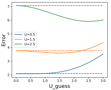
Refer to caption
Figure 6: Simulation Results with A Larger Sample Size. Solid Lines (Dashed Lines) Represent the Proposed Method (Basic Pooling Method).

As part of our additional simulation results related to the comparisons against competing methods in the literature, we consider the same settings in Section 4.2.1 and Section 4.2.2 with a smaller nS/nTn_{S}/n_{T} ratio. In particular, we vary the sample sizes to be nS=200n_{S}=200 and nT=100n_{T}=100. For the methods under consideration, we report the average estimation error of θT\theta_{T} in (5), and its standard deviation, over 10001000 simulation runs. The results are summarized in the left-half of Table 3 for moderate-dimensions and the right-half of Table 3 for high-dimensions. We observe behaviors of our proposed method relative to the competing methods to be consistent with those in Section 4.2.1 and Section 4.2.2.

Table 3: Simulation Results Comparing the Proposed Method to Other Competing Methods in Moderate-Dimensions (Left-Half) and in High-Dimensions (Right-Half). “Basic” Represents the Lowest of the Errors Attained by the Three Basic Methods in Section 2.2. Numbers in Parentheses Are Standard Deviations.
UU Basic Proposed Two-Step Trans-Lasso Basic Proposed Two-Step Trans-Lasso
0.5 6.8(2.1) 7.1(2.2) 10.6(3.6) 1.1(2.4) 33.9(7.2) 30.9(7.6) 61.1(23.7) 34.2(7.5)
1.5 8.4(2.5) 8.5(2.7) 11.4(3.5) 1.7(2.2) 36.3(6.2) 32.6(6.6) 62.9(22.2) 37.4(6.6)
2.5 10.5(2.7) 9.9(2.5) 14.1(4.5) 2.5(2.6) 38.6(5.9) 34.3(6.1) 69.8(22.1) 40.5(6.3)
3.5 13.1(3.2) 11.6(3.1) 15.5(4.6) 4.8(3.4) 44.6(5.6) 38.3(6.4) 77.1(23.7) 47.6(6.0)
4.5 17.5(3.7) 14.5(3.9) 17.6(6.2) 8.7(4.5) 50.8(6.1) 41.5(5.8) 84.8(23.5) 55.2(7.4)
5.5 19.3(5.8) 15.3(4.8) 18.7(7.2) 11.7(4.9) 58.3(7.2) 45.4(8.1) 98.8(24.9) 63.6(8.1)
6.5 19.3(6.4) 17.3(6.0) 19.7(7.7) 16.6(6.6) 55.9(12.5) 49.3(8.7) 115.9(29.4) 74.4(7.5)
7.5 19.4(6.8) 18.3(6.4) 19.3(7.5) 20.4(7.2) 57.1(11.6) 52.9(9.4) 130.3(30.1) 87.3(9.8)
8.5 20.1(5.5) 18.5(6.1) 19.0(6.4) 21.7(9.4) 56.3(12.8) 53.4(10.7) 151.8(28.3) 98.9(9.8)
9.5 21.4(12.4) 18.8(6.9) 20.5(7.6) 23.2(9.0) 57.7(13.9) 56.9(9.6) 167.6(34.5) 112.5(10.8)

B.2 Real-World Dataset Experiments

As part of our final set of empirical results considered in Section 4.2.3, we compare our proposed method against the other competing methods using the Uber&\&Lyft dataset (https://www.kaggle.com/brllrb/uber-and-lyft-dataset-boston-ma) of Uber and Lyft cab rides collected in Boston, MA. Recall that we consider UberX to be the source model and standard Lyft service to be the target model where the learning problem comprises prediction of the price using d=32d=32 numerical features. Given that the focus of our study is on the benefit of transfer learning, we restrict our experiments to small random subsamples and we summarize in Table 2 the results taken over 100100 repeated independent experiments.

The Uber&\&Lyft dataset consists of 55094 observations for the source and 51235 observations for the target, from which we obtain and present in Figures 7 and 8 the corresponding ground-truth regression parameters as bar plots for the source and target models, respectively. We observe that the parameters are moderately sparse with the feature “surge_multiplier” having much larger magnitudes in comparison with the other features. Figure 9 plots the difference between these two parameters, from which we again observe that the difference is sparse. We also compute the lql_{q}-distance, q∈{0,0.5,1}q\in\{0,0.5,1\}, between the source and target parameters and summarize these results in Table 4.

The results in Table 2 show that our proposed method attains a better performance on average, by a small margin relative to the basic methods and by a large margin relative to the two-step estimator and Trans-Lasso. We note that the lql_{q} sparsity, q∈[0,1]q\in[0,1], required by the last two methods does not reasonably capture the contrast between the source and target models of the real-world dataset, due to the moderate dimensions and the existence of one dominating feature In particular, while Bastani 2021 shows that the two-step joint estimator performs well when the difference of regression parameters is l0l_{0} sparse, their result applies to high-dimensions which is in contrast to the 3232 dimensions of the dataset at hand. This helps to explain why their two-step joint estimator does not yield good performance in Table 2 where the moderate dimensions and a single feature of “surge_multiplier” significantly affects the model. Li et al. 2020 show that their Trans-Lasso method performs well when the l1l_{1}-difference of the regression parameters (denoted by h1h_{1}) satisfies h1≪s​log⁡d/nTh_{1}\ll s\sqrt{\log d/n_{T}}, where ss is the l0l_{0} sparsity of the target regression parameters. However, for the real-world dataset, we observe that s≈8s\approx 8 (see Figure 8), that the factor log⁡(d)/nT\sqrt{\log(d)/n_{T}} is smaller than 0.20.2, that hqh_{q} (i.e., lql_{q}-difference of the regression parameters) increases as qq decreases from 11 toward 00, and that hqh_{q} presents a discontinuity at q=0q=0 with h0=8h_{0}=8, some of which is illustrated in Table 4. Hence, the l1l_{1} (or lql_{q} in general) relationship assumed by Li et al. 2020 does not appear to hold for the dataset at hand. This in turn helps to explain why Trans-Lasso does not yield good performance in Table 2.

Refer to caption
Figure 7: Estimated Regression Parameters of Source Model From the Entire Source Dataset.
Refer to caption
Figure 8: Estimated Regression Parameters of Target Model From the Entire Target Dataset.
Refer to caption
Figure 9: Difference in Regression Parameters of Target versus Source Model From the Entire Dataset.
Table 4: Results For Distance (under Different Sparsity Norms) between Source and Target Ground-truth Parameters on Uber&\&Lyft Data. The l0l_{0}-distance Has a Threshold of 0.10.1 to Determine Non-zero Entries.
l0l_{0}-distance (h0h_{0}) l0.5l_{0.5}-distance (h0.5h_{0.5}) l1l_{1}-distance (h1h_{1})
8 189.67 53.65