Self-Consistent Implementation of Kohn-Sham Adiabatic Connection Models with Improved Treatment of the Strong-Interaction Limit
Abstract
Adiabatic connection models (ACMs), which interpolate between the limits of weak and strong interaction, are powerful tools to build accurate exchange-correlation functionals. If the exact weak-interaction expansion from second-order perturbation theory is included, a self-consistent implementation of these functionals is challenging and still absent in the literature. In this work we fill this gap by presenting a fully self-consistent-field (SCF) implementation of some popular ACM functionals. While using second-order perturbation theory at weak interactions, we have also introduced new generalised gradient approximations (GGA’s), beyond the usual point-charge-plus-continuum model, for the first two leading terms at strong interactions, which are crucial to ensure robustness and reliability. We then assess the SCF-ACM functionals for molecular systems and for prototypical strong-correlation problems. We find that they perform well for both the total energy and the electronic density and that the impact of SCF orbitals is directly connected to the accuracy of the ACM functional form. For the H2 dissociation the SCF-ACM functionals yield significant improvements with respect to standard functionals, also thanks to the use of the new GGA’s for the strong-coupling functionals.
1 Introduction
Kohn-Sham (KS)Kohn and Sham 1965 density functional theory (DFT) is the most used electronic structure computational approach for molecular and solid-state systemsBurke 2012; Becke 2014; Jones 2015. Its accuracy depends on the choice of the approximation for the exchange-correlation (XC) functional Scuseria and Staroverov 2005; Mardirossian and Head-Gordon 2017; Della Sala et al. 2016 which, at the highest-rung of the Jacob’s ladderPerdew and Schmidt 2001, involves all the occupied and virtual KS orbitals as well as the eigenvalues. Then, the XC approximation is no more an explicit functional of the density and, to stay within the pure KS formalism, the optimized effective potential (OEP) method Engel 2003; Kümmel and Kronik 2008 must be employed. Early OEP approaches included exact-exchange (EXX) and approximated the correlation using the second-order Görling-Levy perturbation theory (GL2) Görling and Levy 1994. However this led to a large overestimation of correlation effects and to convergence problems Grabowski et al. 2002; Bartlett et al. 2005; Jiang and Engel 2005; Schweigert et al. 2006; Mori-Sánchez et al. 2005; Grabowski et al. 2011; Grabowski et al. 2007.
Actually two different main approaches have been explored to solve this issue: going beyond the second-order approximation Verma and Bartlett 2012; Furche 2008; Grüneis et al. 2009; Heßelmann and Görling 2010; Heßelmann and Görling 2011; Bleiziffer et al. 2013; Bleiziffer et al. 2015; Zhang et al. 2016 or using a semicanonical trasformation Grabowski et al. 2002; Bartlett et al. 2005; Grabowski et al. 2007 . Another possible path is the adiabatic connection (AC) formalism Langreth and Perdew 1975; Gunnarsson and Lundqvist 1976; Savin et al. 2003 which is a general, powerful tool for the development of XC functionals. For several decades it has been used to justify the introduction of hybrid Becke 1993; Perdew et al. 1996; Fabiano et al. 2015 and double hybrid (DH) functionals Sharkas et al. 2011; Brémond and Adamo 2011; Brémond et al. 2016 and successively it has been directly employed to construct high-level XC functionals based on AC models (ACM) interpolating between known limits of the AC integrand Seidl et al. 2000; Seidl et al. 2005; Seidl et al. 2000; Gori-Giorgi et al. 2009; Seidl et al. 1999; Liu and Burke 2009; Ernzerhof 1996; Teale et al. 2010. Recently it has also been employed in the context of the Hartree-Fock (HF) theory Seidl et al. 2018; Daas et al. 2020 to develop corrections to the Møller-Plesset perturbation series Daas et al. 2021.
The XC functionals based on ACMs have the general form
| (1) |
where , with being the exact exchange energy, being twice the GL2 correlation energy Görling and Levy 1994, and and being the indirect part of the minimum expectation value of the electron-electron repulsion for a given density and the potential energy of coupled zero-point oscillations around this minimum, respectively Seidl et al. 2007; Gori-Giorgi et al. 2009. The model is designed to mimic the exact but unknown , in particular by considering the known asymptotic expansions Gori-Giorgi et al. 2009; Seidl et al. 1999; Görling and Levy 1994; Seidl et al. 2007
| (2) | |||||
| (3) |
In recent years several ACMs have been tested for various chemical applications showing promising results Fabiano et al. 2016; Giarrusso et al. 2018, especially in the description of non-covalent interactions Daas et al. 2021; Vuckovic et al. 2018. However, most of these recent studies have been performed within the HF-AC framework, i.e. as post-HF calculations. Conversely, little attention has been devoted to DFT-based ACM functionals. The main reason for this is that in the HF case the ACM is applied on top of the HF ground state Seidl et al. 2018; Daas et al. 2020, which is a simple and well defined reference; on the contrary, in the DFT framework the ACM-based XC functional should be in principle applied inside the KS equations in a self-consistent-field (SCF) fashion. This requirement is not trivial because ACM-based functionals are in general not simple explicit functionals of the density but are instead complicated expressions depending on KS orbitals and orbital energies as well (through and ). One notable exception are the MCY functionals Cohen et al. 2007 which use semilocal approximations to set the interpolation points along the AC integrand, thus allowing for a relatively straightforward SCF implementation. In the most general case considered in this work, however, ACM functionals are fifth rung functionals thus, in practice, also in the context of DFT, they are always applied in a post-SCF scheme using precomputed DFT densities and orbitals Fabiano et al. 2016; Śmiga and Constantin 2020. In this way the results depend significantly on the choice of the reference density and orbitals, making the whole method not fully reliable Fabiano et al. 2016. On the other hand, an exploratory study of the XC potential derived from ACM models has shown that this possesses promising features, indicating that SCF calculations with ACM-based functionals might be an interesting path to explore Fabiano et al. 2019.
In this work we tackle this issue by introducing an SCF implementation of the ACM potential and applying it to some test problems in order to verify its ability to describe different properties and systems. One important aim of this work is in fact to measure and assess the capabilities of some of the most popular ACM presently available in literature. To this purpose the use of a proper SCF procedure is crucial as the level of accuracy of such methods can be inspected independently of an arbitrary reference ground-state as in previous works. In fact, for any density functional the energy error can be decomposed into a contribution due to the approximate nature of the functional (intrinsic error) and that due to the approximate density used in the calculation (relaxation error) Kim et al. 2013; Sim et al. 2022. When the functional is evaluated on an arbitrary (non-SCF) density, the relaxation error may become important and the whole performance can be influenced by the choice of the density. Indeed, recent studies have shown how this effect can be used to improve DFT results by choosing accurate non-SCF densities Sim et al. 2022; Li Manni et al. 2014. Nevertheless, within this framework its difficult to really understand the accuracy of the functional form itself and therefore to plan new advances. On the other hand, the use of a proper SCF procedure provides a well defined reference for assessing the intrinsic errors. This is an extremely important point to clarify in view of future ACM developments. Note that such a development of new and possibly more accurate ACMs will instead not be covered in this work but left to upcoming publications. The development work performed here will instead focus an a second important goal aimed at solving some open problems with the ACM potential that hinder its straightforward SCF implementation. These problems originate mainly from the naive treatment used so far for the large- contributions and which causes an unphysical behavior in the ACM potential. Hence, in this article we develop new approximations for both and that preserve the accuracy for energies and remove the limitations on the potential side. As a byproduct of this work we obtain useful strong-correlation generalized gradient approximations that prove to be very robust for the description of the Harmonium atom and the H2 dissociation.
In the following, we present the theory behind SCF implementation of ACM functionals and the construction of new and approximations. Afterwards, we present some interesting preliminary results obtained for model and real systems.
2 Theory
To perform SCF ACM calculations we need to deal with the potential arising from the functional derivative of the energy of Eq. (1), that is Fabiano et al. 2019
| (4) | |||||
where with , , , . As discussed in Ref. 53, the potential in Eq. (4) requires a combination of OEP (for and ) and GGA approaches (for and ). Thus it resembles the OEP-SCF implementation of the DH functionals reported in Ref. 57; 58. In more details, the and functional derivatives are obtained via solving the OEP equation which readsSharp and Horton 1953; Talman and Shadwick 1976; Grabowski et al. 2002; Kümmel and Kronik 2008; Della Sala 2011; Engel 2003
| (5) |
with denoting the exchange and correlation parts, respectively. The inhomogeneity on the right hand side of Eq. (5) is given by
| (6) | |||||
and the static KS linear response function
| (7) |
All quantities are evaluated using orbitals and eigenvalues in a given cycle of KS SCF procedure. (Further details can be found in Refs. 17; 62; 63; 57; 58). We note, however, that there is a significant difference between ACM and DH approaches: in the former the coefficients and are not fixed empirical parameters as in DH, but are well defined (non-linear) functions of Fabiano et al. 2019.
2.1 Approximations for the strong-interaction limit
Another important issue to consider in the SCF implementation of the ACMs is related to the treatment of and , which describe the limit of the AC integrand. It can be proven that both and display a highly non-local density dependence.Buttazzo et al. 2012; Cotar et al. 2013; Cotar et al. 2018; Lewin 2018; Colombo et al. 2021 This is accurately described by the strictly-correlated electrons (SCE) formalism, Seidl et al. 2007; Gori-Giorgi et al. 2009 which is however computationally very demanding and non trivial to evaluate. Therefore, the limit is usually approximated by simple semilocal gradient expansions (GEA) derived within the point-charge-plus-continuum (PC) model Seidl et al. 2000
| (8) | |||||
| (9) |
where is the reduced gradient of the density, , , , and (slightly different estimates are possible for , see e.g. Refs. 36; 39). The GEAs of Eqs. (8) and (9) yield, at least for small atoms, energies that are quite close to the accurate SCE values. However, when is large, e.g. in the tail of an exponentially decaying density, they fail, giving functional derivatives that diverge.Fabiano et al. 2019 This is a severe drawback that does not allow these approximations to be used directly in an SCF implementation.
To remedy this limitation we consider here a simple GGA approximation, named harmonium PC (hPC) model, based on the Perdew-Burke-Ernzerhof (PBE) exchange enhancement factor Perdew et al. 1996, that recovers the GEAs of Eqs. (8) and (9) in the slowly-varying regime, is well behaved everywhere, and reproduces as close as possible the SCE values for both and . Thus, we have
| (10) | |||||
| (11) |
where and have been fixed such that and recover exactly the corresponding SCE values for the harmonium atom at Kooi and Gori-Giorgi 2018: with this value the degree of correlation resembles that of the He atom and a simple analytical density is obtained. We note that a previous attempt to develop GGA’s for and , the modified PC (mPC) model of Ref. 71, yields results that are quite far from both the PC and the SCE values, in particular does not even recover the PC model in the small limit. In fact, the mPC GGAs have been derived for the quasi-two-dimensional density regime Constantin 2019 and their application in three-dimensional systems, e.g. for the total correlation of atoms, is highly based on an error cancellation between the quite inaccurate values of and . Constantin 2019 In particular, has been designed to compensate the inaccuracies of for the ISI functional, but this error compensation cannot work for other ACMs (especially those, as SPL, using only ).
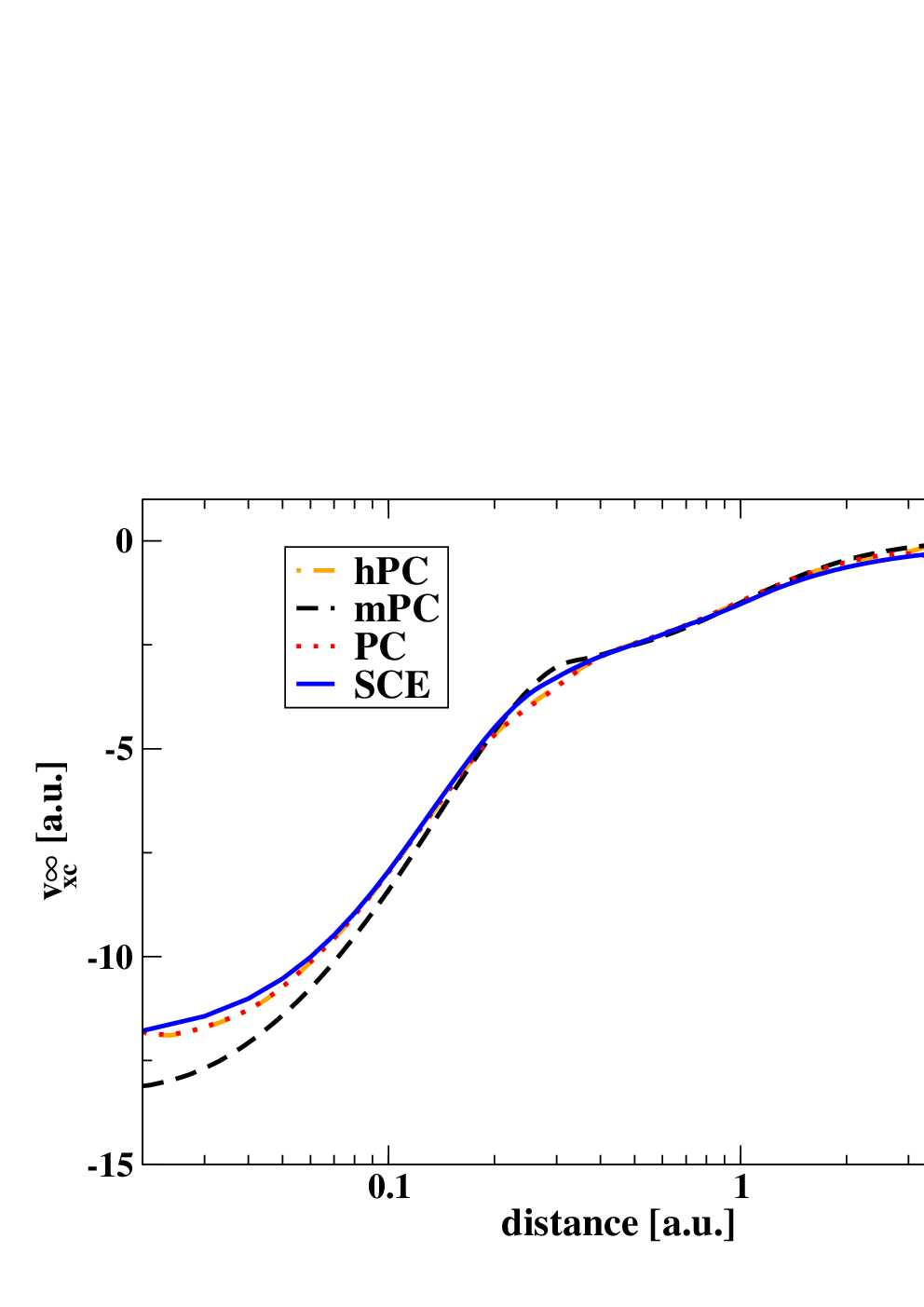
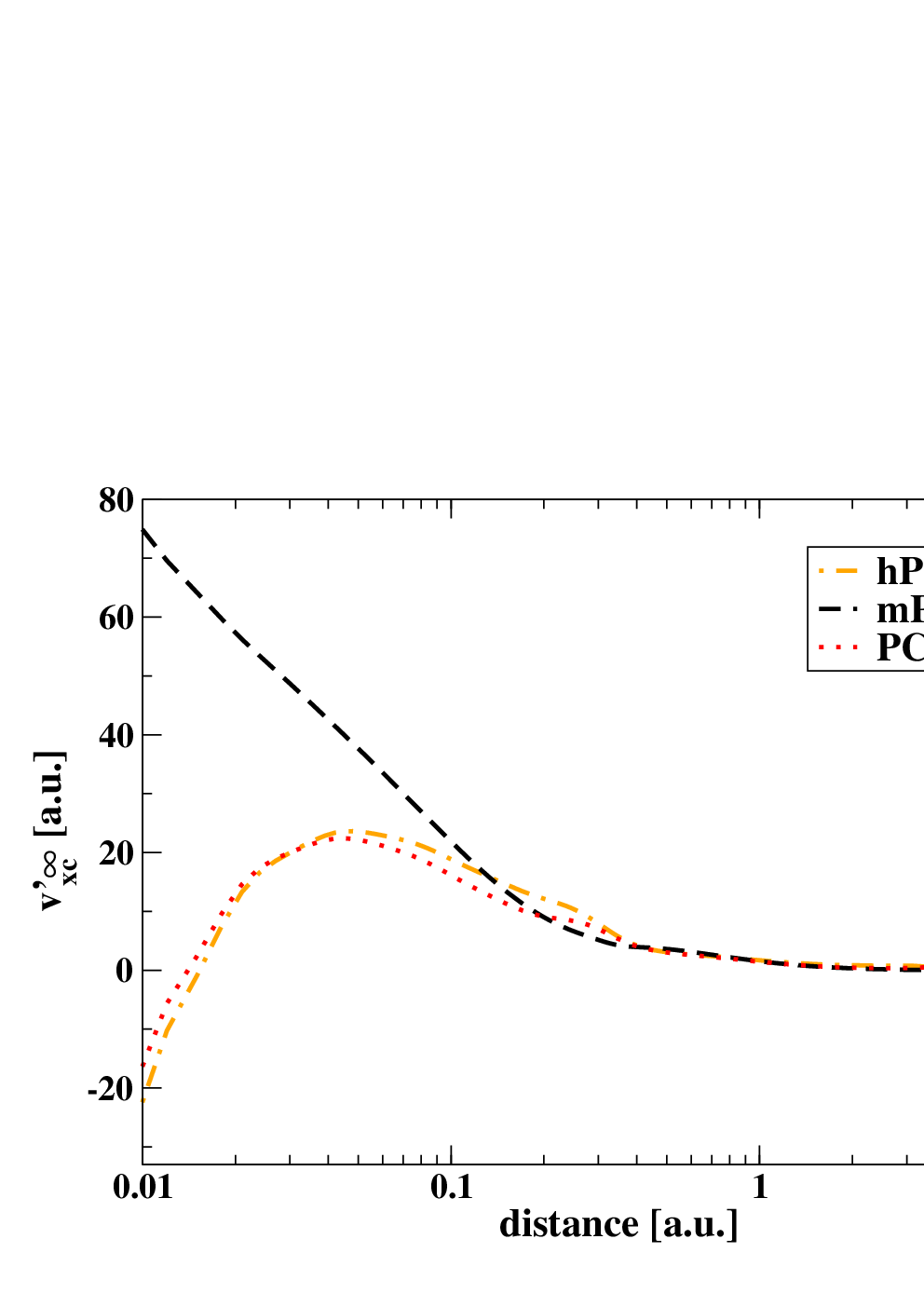
To understand the performances of the different approximations for the strong-interaction functionals, we report in Fig. 1 the differences between the values of and computed with the two GGA’s and the PC model, for the Hooke atom at different confinement strengths . The corresponding values for those instances of for which exact SCE reference data are available are also reported in Table 1.
| SCE | PC | hPC | mPC | |
| 0.0365373 | -0.170 | -0.156 | -0.167 | -0.191 |
| 0.1 | -0.304 | -0.284 | -0.303 | -0.344 |
| 0.5 | -0.743 | -0.702 | -0.743 | -0.841 |
| MARE | 6.78% | 0.70% | 12.90% | |
| 0.0365373 | 0.022 | 0.021 | 0.021 | 0.060 |
| 0.1 | 0.054 | 0.054 | 0.053 | 0.146 |
| 0.5 | 0.208 | 0.215 | 0.208 | 0.562 |
| MARE | 2.64% | 2.13% | 171.10% | |

We see that, unlike mPC, the hPC model reproduces very well both the and accurate SCE values,Kooi and Gori-Giorgi 2018 being comparable to and even superior to the original PC model. This performance is not trivial since hPC was parameterized only on a single instance of the Hooke’s atom () but turns out to be very accurate for the whole range of confinement strengths. In particular, Figure 2 shows that in the small range (strong interaction limit of the Hooke’s atom) hPC yields the best estimation of the XC energy , being slightly better than PC, while the mPC method fails completely.

An additional assessment is provided in Table 2 and Fig. 3 where real atoms are considered both for SCE energies and SCE potentials. Also in this case the results of the hPC functional are in line with or better than the PC model, that was originally parametrized against the He atom, indicating once more the robustness of the hPC method. As anticipated the mPC is instead quite far from the reference, especially for .
| SCE | PC | hPC | mPC | |
| H | -0.3125 | -0.3128 | -0.3293 | -0.4000 |
| He | -1.500 | -1.463 | -1.492 | -1.671 |
| Be | -4.021 | -3.943 | -3.976 | -4.380 |
| Ne | -20.035 | -20.018 | -20.079 | -21.022 |
| MARE | 1.15% | 1.81% | 13.31% | |
| H | 0 | 0.0426 | 0.0255 | 0.2918 |
| He | 0.621 | 0.729 | 0.646 | 1.728 |
| Be | 2.59 | 2.919 | 2.600 | 6.167 |
| Ne | 22 | 24.425 | 23.045 | 38.644 |
| MARE | 13.71% | 3.05% | 130.67% | |
3 Computation details
All calculations have been performed with a locally modified ACESII Stanton et al. 2007 software package. As in our previous studiesŚmiga et al. 2016; Śmiga et al. 2020; Grabowski et al. 2011; Śmiga et al. 2016; Grabowski et al. 2014; Fabiano et al. 2019; Śmiga et al. 2020; Śmiga et al. 2020 in order to solve OEP equations we have employed the finite-basis set procedure of Refs. 77; 78. In calculations we employed the basis sets detailed below and tight convergence criteria (SCF: ). In general, the convergence criteria were met within several cycles of SCF procedure.
In order to solve algebraic OEP equations, the truncated singular-value decomposition (TSVD) of the response matrix was employed. The cutoff criteria in the TSVD procedure was set to . For technical details on this type of calculations we refer the reader to Refs. 17; 63.
As reference data we have considered the coupled-cluster single double and perturbative triple [CCSD(T)]Raghavachari et al. 1989 results obtained in the same basis set, in order to make a comparison on the same footing and to reduce basis set related errors. In particular, we have considered a comparison with CCSD(T) relaxed densities, the corresponding KS potentials obtained via KS inversionWu and Yang 2003 and the total CCSD(T) energies. In the assessment we have considered several properties i.e.:
- -
total energies: the total energies have been calculated for the systems listed in Table I in Ref. 63 using identical computational setup as in the same paper. A summary of the employed basis sets is also reported in the Supporting Information. We remark that, although total energies are not very important in practical chemical applications, they are important observables and are especially useful as indicators of the quality of the ACM interpolation.
- -
Dipole moments: for selected systems (H2O, HF, HCl, H2S, CO) we have calculated the dipole moments using SCF densities for various methods. This is a direct test of the quality of self-consistent densities obtained within all approaches. The uncontracted aug-cc-pVTZ basis set of Dunning Kendall et al. 1992 was used for all systems together with geometries taken from Ref. 82.
- -
HOMO and HOMO-LUMO gap energies: as in Ref. 83 and Ref. 63 we have computed the HOMO and HOMO-LUMO gaps, respectively, for the same set of systems as in the case of total energies. In the case of HOMO energies, the reference data have been taken from Ref. 83 whereas the HOMO-LUMO gap energies have been obtained from applying the KS inversion method Wu and Yang 2003 taking as a starting point the CCSD(T) relaxed density matrix as in Ref. 63.
- -
correlation potentials and densities: as in our previous studiesGrabowski et al. 2011; Grabowski et al. 2014; Grabowski et al. 2014; Śmiga et al. 2014 , also here we investigate the quality of correlation potentials and densitiesJankowski et al. 2009; Jankowski et al. 2010; Grabowski et al. 2011 looking at their spatial behavior. Both quantities are obtained from fully SCF calculations. The densities are analyzed in term of correlation densities defined as , where is the density obtained from the exact exchange only (X=EXX)Talman and Shadwick 1976 or Hartree-Fock (HF) (X=HF) calculations, for DFT and WFT methods, respectively. The Ne atom OEP calculations have been performed in fully uncontracted ROOS-ATZP Widmark et al. 1990 basis set whereas for CO molecule the uncontracted cc-pVTZ Dunning 1989 basis sets was employed.
- -
dissociation of H2: fully self-consistent and post-SCF calculations, using OEP EXX orbitals, have been performed in the spin restricted formalism using the uncontracted aug-cc-pVTZ basis set. For comparison PBE, MP2, GL2@EXX and FCI data are also reported.
- -
correlation energies of Hooke’s atoms: as previouslyŚmiga and Constantin 2020; Jana et al. 2020; Jana et al. 2021 we have performed calculation for various values of in the Hooke’s atom modelKestner and Sinanoḡlu 1962 ranging between 0.03 (strong interaction) to 1000 (weak interaction) using a even-tempered Gaussian basis set from Ref. 93. For comparison, the ACM correlation energies have been calculated at both @EXX and @SCF reference orbitals.
4 Results
We have performed a series of SCF ACM calculations to investigate the performance of these methods in the KS framework. In particular, we have considered the Interaction-Strength-Interpolation (ISI)Seidl et al. 2000 and Seidl-Perdew-Levy (SPL)Seidl et al. 1999 ACMs. Unless explicitly stated, the hPC model has been used to describe the strong-interaction limit in all calculations. Moreover the bare GL2 (for SCF calculations OEP-GL2 Grabowski et al. 2002) approach is also reported. The ISI model for has in general a larger deviation from linearity than SPL (which does not depend on too), whereas GL2 corresponds to the linear approximation . Thus the comparison of ISI with SPL and GL2 gives information on the importance of the shape of the ACM interpolation form.
In Table 3 we show the total energies computed with the various methods for a test set of 16 closed-shell atoms and small molecules, namely He, Be, Ne, Mg, Ar, HF, CO, H2O, H2, He2,Cl2,N2,Ne2,HCl,NH3 ,C2H6.
| @SCF | @EXX | |||||||
|---|---|---|---|---|---|---|---|---|
| System | ISI | SPL | GL2 | ISI | SPL | GL2 | CCSD(T) | |
| He | -2.90089 | -2.90043 | -2.90780 | -2.90191 | -2.90148 | -2.90925 | -2.90253 | |
| Be | -14.67318 | -14.67551 | not. conv. | -14.67102 | -14.67278 | -14.69013 | -14.66234 | |
| Ne | -128.93274 | -128.94313 | -128.98863 | -128.92733 | -128.93628 | -128.97770 | -128.89996 | |
| Mg | -199.86915 | -199.86937 | -199.88275 | -199.86560 | -199.86569 | -199.87826 | -199.82815 | |
| Ar | -527.51661 | -527.53309 | -527.58461 | -527.51478 | -527.53095 | -527.58181 | -527.45748 | |
| H2 | -1.17039 | -1.16972 | -1.18107 | -1.17019 | -1.16953 | -1.18060 | -1.17273 | |
| He2 | -5.80177 | -5.80086 | -5.81560 | -5.80167 | -5.80075 | -5.81539 | -5.80506 | |
| N2 | -109.58263 | -109.61715 | -109.75090 | -109.56105 | -109.58609 | -109.68725 | -109.47628 | |
| Ne2 | -257.86564 | -257.88644 | -257.97751 | -257.85475 | -257.87266 | -257.95552 | -257.80003 | |
| HF | -100.43787 | -100.45019 | -100.50368 | -100.43148 | -100.44188 | -100.48965 | -100.39579 | |
| CO | -113.35397 | -113.38496 | -113.51191 | -113.32766 | -113.34760 | -113.43484 | -113.25738 | |
| H2O | -76.42686 | -76.44091 | -76.50285 | -76.42076 | -76.43270 | -76.48790 | -76.38692 | |
| HCl | -460.58531 | -460.58876 | -460.61411 | -460.58227 | -460.58550 | -460.61020 | -460.50933 | |
| Cl2 | -919.93674 | -919.94378 | -919.99349 | -919.92413 | -919.93022 | -919.97763 | -919.77032 | |
| NH3 | -56.55283 | -56.56435 | -56.62446 | -56.54859 | -56.55876 | -56.61412 | -56.52332 | |
| C2H6 | -79.80517 | -79.82045 | -79.92279 | -79.79876 | -79.81239 | -79.90830 | -79.76414 | |
| ME | -50.00 | -61.08a | -120.85 | -43.14 | -52.09 | -99.17 | ||
| MAE | 50.91 | 62.25a | 120.85 | 43.96 | 53.16 | 99.17 | ||
| MARE | 0.055% | 0.071%a | 0.162% | 0.048% | 0.062% | 0.150% | ||
not. conv. - not converged; a without Be.
We see that ISI@SCF and SPL@SCF perform quite well, giving errors roughly half that of OEP-GL2. For comparison we acknowledge that the PBE functional Perdew et al. 1996 yields a MARE of 0.11%, which is twice as large as that of ISI@SCF.
Nevertheless, we have to acknowledge that the performance has further margins of improvement. For example the MAEs of MP2 and OEP2-sc (not reported) for the same test are 20 mHa and 17 mHa, respectively. We can trace back most of this difference to the fact that the use of KS eigenvalues, as in ISI, SPL and OEP-GL2, requires a quite large AC curvature (i.e. second derivative with respect to ) to yield accurate results, whereas this is not the case for MP2 and OEP2-sc that employ HF-quality eigenvalues. Then, KS based methods need much more accurate ACMs to compete with HF based ones. This is also confirmed observing that in Tab. 3, ISI is generally better than SPL, as the former is a more advanced ACM than the latter.
A second, related observation is that the ISI and SPL results suffer from a small relaxation error that worsens slightly the performance (with respect using EXX orbitals). This effect might be related to the fact that the considered ACMs were developed in the context of post-SCF calculations and, as a result, may include some inherent error cancellation which is lost when they are evaluated using a (more accurate) SCF density. To understand better this trend we define the quantity
| (12) |
which considers the absolute error difference (with respect the reference, i.e. CCSD(T)) going from EXX orbitals to SCF orbitals (a negative value means that SCF orbitals give better accuracy than EXX orbitals). The values of for ISI, SPL and OEP-GL2/GL2 are 7.0, 9.1 and 16.9 mHa, respectively. Despite the values all being positive (i.e. calculations using EXX orbitals are more accurate) they decrease going from GL2 to SPL and then from SPL to ISI, showing again that increasing the complexity/accuracy of the ACM can yield better SCF potentials and relaxed total energies.
Interestingly an opposite effect of the density relaxation is found in the harmonium atom, as shown in Fig. 4, where if we look at small values of the confinement strength, where the relaxation becomes more important, the SCF results are better with respect to the ones obtained using EXX orbitals and density (for both ISI and SPL) . This depends on the fact that at these regimes the true density is very different from the EXX one and thus the SCF procedure produces a significant improvement on the density. This also traces back to the use of hPC which yields accurate strong-correlation potentials; we note in fact that the accuracy of both ACMs with the hPC model is very high (compare e.g. with Figure 3 of Ref. 52). Conversely using the mPC model only ISI results are rather accurate, because of error compensation effects between the and the terms, while SPL ones, where only is used, are rather poor (see Fig. S2 in the Supporting Information). This is an important indication of the importance of using proper strong-correlation approximations, delivering both good energies and potentials.

In Table 4 we report the dipole moments of some selected systems, from the SCF density. The results for CO are reported separately because they are qualitatively different and deserve a distinct analysis.
| Method | H2O | HF | HCl | H2S | MAE | CO | |
|---|---|---|---|---|---|---|---|
| CCSD(T) | Exp. | ||||||
| OEPx | 2.043 | 1.954 | 1.279 | 1.171 | 0.121 | 0.180 | -0.265 |
| GL2 | 1.616 | 1.531 | 1.061 | 1.004 | 0.187 | 0.145 | 1.703 |
| SPL | 1.758 | 1.654 | 1.085 | 1.024 | 0.110 | 0.080 | 0.940 |
| ISI | 1.809 | 1.699 | 1.093 | 1.030 | 0.083 | 0.060 | 0.692 |
| OEP2-sc | 1.885 | 1.786 | 1.185 | 1.094 | 0.018 | 0.073 | 0.355 |
| CCSD(T) | 1.904 | 1.809 | 1.170 | 1.079 | 0.065 | 0.153 | |
| Exp. | 1.855 | 1.820 | 1.080 | 0.970 | 0.122 | ||
For H2O, HF, HCl, and H2S, a comparison with the CCSD(T) data shows that ISI is quite effective in predicting the dipole moments being slightly better than SPL and twice as good as GL2 (for comparison PBE give in this case a MAE of 0.092 Debye with respect CCSD(T)). Anyway, as already observed for the total energies, there are important margins of improvement as testified by the OEP2-sc performance that is definitely better than the ISI one. As already discussed we can trace back the limitations of ISI and SPL in part to relaxation effects but also on the fact that, working in a pure SCF KS framework, it is very hard for the ACM to provide a proper curvature of the AC integrand curve as to get accurate KS orbital energies; consequently the orbital-dependent energies are also negatively affected. For the case of CO these effects are even more evident. In this case in fact OEPx predicts a qualitatively wrong dipole moment but GL2 largely over-corrects it, indicating that the linear behavior of the AC integrand needs to be significantly improved. Both ISI and SPL can partially achieve this task, halving the error with respect to GL2, but still they yield quite overestimated dipole moments.
| @SCF | |||||||
|---|---|---|---|---|---|---|---|
| System | OEPx | GL2 | OEP2-sc | SPL | ISI | KS[CCSD(T)] | |
| He | 21.60 | 20.95 | 21.32 | 21.23 | 21.23 | 21.21 | |
| Be | 3.57 | not. conv. | 3.63 | 3.40 | 3.47 | 3.61 | |
| Ne | 18.48 | 14.12 | 16.45 | 15.17 | 15.60 | 17.00 | |
| Mg | 3.18 | 3.40 | 3.33 | 3.38 | 3.38 | 3.36 | |
| Ar | 11.80 | 10.95 | 11.43 | 11.08 | 11.17 | 11.51 | |
| H2 | 12.09 | 12.03 | 12.13 | 12.12 | 12.12 | 12.14 | |
| He2 | 21.28 | 20.64 | 21.02 | 20.81 | 20.81 | 20.56 | |
| N2 | 9.21 | 6.73 | 8.37 | 7.68 | 7.99 | 8.55 | |
| Ne2 | 17.84 | 13.49 | 15.75 | 14.41 | 14.83 | 16.23 | |
| HF | 11.36 | 7.80 | 9.84 | 8.70 | 9.08 | 10.30 | |
| CO | 7.77 | 5.87 | 7.22 | 6.68 | 6.90 | 7.29 | |
| H2O | 8.44 | 5.99 | 7.49 | 6.73 | 7.03 | 7.75 | |
| HCl | 7.82 | 7.10 | 7.52 | 7.11 | 7.14 | 7.55 | |
| Cl2 | 3.90 | 2.65 | 3.35 | 2.74 | 2.78 | 3.29 | |
| NH3 | 6.97 | 5.30 | 6.35 | 5.78 | 5.98 | 6.54 | |
| C2H6 | 9.21 | 8.24 | 8.85 | 8.51 | 8.62 | 8.95 | |
| ME | +0.54 | -1.13a | -0.11 | -0.64 | -0.48 | ||
| MAE | 0.52 | 1.15a | 0.21 | 0.68 | 0.52 | ||
| MARE | 6.49 | 12.16%a | 1.86% | 7.49% | 5.71% | ||
not. conv. - not converged; a without Be.
| @SCF | ||||||
|---|---|---|---|---|---|---|
| System | OEPx | GL2 | OEP2-sc | SPL | ISI | CCSD(T) |
| He | -24.98 | -24.23 | -24.55 | -24.46 | -24.39 | -24.48 |
| Be | -8.41 | not. conv. | -8.89 | -9.47 | -9.32 | -9.31 |
| Ne | -23.38 | -17.66 | -20.14 | -18.98 | -19.48 | -21.47 |
| Mg | -6.88 | -8.04 | -7.33 | -7.93 | -7.91 | -7.57 |
| Ar | -16.08 | -14.94 | -15.34 | -15.11 | -15.20 | -15.63 |
| H2 | -16.17 | -16.34 | -16.30 | -16.25 | -16.13 | -16.41 |
| He2 | -24.92 | -24.14 | -24.47 | -24.38 | -24.30 | -24.48 |
| N2 | -17.17 | -11.32 | -15.65 | -13.09 | -13.78 | -15.51 |
| Ne2 | -23.05 | -17.45 | -19.98 | -18.80 | -19.31 | -21.34 |
| HF | -17.48 | -12.16 | -14.57 | -13.52 | -14.03 | -15.96 |
| CO | -15.02 | -10.64 | -13.21 | -12.18 | -12.70 | -13.94 |
| H2O | -13.69 | -9.01 | -11.27 | -10.39 | -10.87 | -12.50 |
| HCl | -12.92 | -11.94 | -12.28 | -12.04 | -12.08 | -12.59 |
| Cl2 | -12.06 | -9.92 | -10.85 | -10.14 | -10.22 | -11.45 |
| NH3 | -11.56 | -8.37 | -9.91 | -9.34 | -9.65 | -10.78 |
| C2H6 | -13.21 | -11.39 | -12.20 | -11.93 | -12.07 | -13.01 |
| ME | -0.65 | +1.97a | +0.59 | +1.15 | +0.93 | |
| MAE | 0.89 | 2.49a | 0.62 | 1.22 | 0.98 | |
| MARE | 6.12% | 13.68%a | 4.36% | 8.28% | 6.67% | |
not. conv. - not converged; a without Be.
As a next step, we consider in Table 5 the HOMO-LUMO gaps obtained from different methods. As it could be expected both ACMs correct the general overestimation of gaps given by the OEPx but in doing so they overestimate the correlation effects yielding gaps that are too small in most cases. Thus we obtain MAEs of 0.68 and 0.52 eV for SPL and ISI, respectively, to be compared with the OEP2-sc MAE of 0.21 eV. We note anyway that the ISI and SPL results are clearly better than conventional semilocal functionals (PBE gives a MAE of 0.97 eV). Moreover, we note that by improving the quality of the ACM (GE2SPLISI) the description of the HOMO-LUMO gap is also significantly improved. Similar considerations apply as well for the HOMO energies (see Table 6). At the ISI level, the HOMO is shifted to higher energy with the almost the same MARE as OEPx (which is shifted to lower energy). Again the ISI approach is better than SPL and much better than GL2 (as well as PBE with a MARE of 38.3%.)
Then, we consider the correlation potentials for two typical systems, the Ne atom and the CO molecule. In the top panels of Fig. 5 we see that the ACMs provide a quite good description of the correlation potential for the two systems, improving significantly over GL2. Nevertheless, with respect to reference data there are still some limitations, e.g. a moderate overestimation of the correlation potential in valence regions. This characteristic corresponds to an overestimation of shell oscillations in the SCF density, as indicated in the bottom panels of Fig. 5, where we report the correlation density , i.e. the difference between the density obtained with a correlated method and its exchange-only version.
In the central panels of Fig. 5, we report the values , which is defined, in analogy to Eq. (12) as
| (13) |
These show, point-by-point whether or not the SCF procedure improves the correlation potential with respect to EXX orbitals. As we found for energies, the SCF correlation potentials are less accurate, but the error reduces with more accurate ACM functionals. This feature is also evident for the correlation density, see bottom panels. In this context, we should however also point out that the ACM-SCF density does not correspond to the exact linear response density Voora et al. 2019; Jin et al. 2020; Yu et al. 2021.

As a final case we consider in Fig. 6 the potential energy surface for the dissociation of the H2 molecule, in a restricted formalism Cohen et al. 2012, which is one of the main DFT challenges Cohen et al. 2012; Kirkpatrick et al. 2021, and was previously investigated in the ACM framework Peach et al. 2007; Teale et al. 2009; Teale et al. 2010. While both MP2 and GL2@EXX diverge at large distances, ISI@SCF nicely reproduces the exact FCI curve, much better than ISI@EXX, see also Ref. 48. Thus the SCF procedure turns out to be quite important showing that, despite some limitations discussed above, it is crucial to include important correlation effects into the orbitals. For SPL (see Fig. S1 in the Supporting Information) similar trends are found the SPL@SCF curve for first increases and then decreases asymptotically, a behaviour which is clearly incorrect and depends on some drawbacks of the SPL functional to describe the limit for large distances, which is more influenced by the strong correlation..

The limit for very large distances, well beyond , is numerically tricky, but it can be computed exactly using the hydrogen atom with fractional spins, H(1/2,1/2), i.e. with half spin up and half spin down Cohen et al. 2008. For this system we have so that the ISI XC energy reduces to Seidl et al. 2000
| (14) |
with . The potential is thus a simple linear combination of the EXX potential and the GGA potential from and . For the SPL approach, we have simply that and thus the potential is just .
The errors for different methods and orbitals are reported in Tab. 7.
| @EXACT | @SCF | IDD | |
| PBE | 54.7 | 51.5 | 0.103 |
| EXX | 196.1 | 178.6 | 0.260 |
| SPL-PC | -0.4 | - | - |
| SPL-mPC | -109.8 | -114.9 | 0.125 |
| SPL-hPC | -21.0 | -21.4 | 0.024 |
| ISI-PC | 27.4 | - | - |
| ISI-mPC | 90.2 | 83.7 | 0.151 |
| ISI-hPC | 23.6 | 19.4 | 0.107 |
At the exact density () SPL-PC gives an extremely accurate total energy but the same method fails for the SCF calculation. The SPL-mPC approach strongly underestimate the total energy, while the SPL-hPC gives a much lower error, both for the exact and the SCF densities. At the ISI level all the energies are higher and the ISI-hPC@SCF is the most accurate approach. Note, however, that ISI-PC can be made exact with a proper choice of the parameters Seidl et al. 2000. Note also that EXX fails for this system and PBE is also quite inaccurate. When SCF effects are considered, When SCF effects are considered, PBE, EXX, ISI-mPC, and ISI-hPC yield a slight improvement with respect to the case when the exact density is used. Because the integrated density difference (IDD) is not zero in all cases, this is a clear signature that all methods display some error compensation effect. Moreover, some methods give important convergence issues: the simple PC model does not converge, as explained above; the mPC model converges but the errors are very large, about twice the PBE ones. Instead, the ISI-hPC is very good for both the considered densities, having the best accuracy among all functionals and performing even better than all the functionals considered in Tab. 5 of Ref. 97. Note that the good accuracy of the ISI-hPC with respect to ISI-mPC is not related to the previously mentioned error cancellation between an incorrect SCF density and an incorrect energy. In fact, the IDD error is significantly smaller going from ISI-hPC to ISI-mPC. Interestingly, the same arguments hold when comparing SPL-hPC to SPL-mPC, thus confirming the high quality of the hPC functional. Note that the almost vanishing IDD value for the SPL-hPC approach is a particular case, and all methods with show a quite accurate density. The accuracy of the ISI-hPC@SCF approach for the H2 dissociation limit is thus quite significant, considering that it uses full exact exchange and a combination of GL2 and a GGA functional without empirical parameters, in contrast to other approaches that use more complex constructions or extensive fitting on molecular data Zhang and Xu 2021; Kirkpatrick et al. 2021.
5 Conclusions
In this paper we have shown that it is possible to use ACM-based XC functionals in a full SCF procedure. This solves a long-standing issue in DFT as all the previous calculations with ACM functionals had been done in a post-SCF fashion using GGA or exact-exchange orbitals. This opens the way to new applications and even basic studies in this context, removing the need for a post-SCF procedure and all the related sources of inaccuracy. Of course, despite the ACM-SCF procedure presented here is well defined, conceptually clean and fully capable of producing important results, is it fair to state that the whole method is not yet optimized and straightforward to apply especially because it is strictly related to the OEP approach used for the treatment of the GL2 component, which requires itself some expertise to be handled. Nevertheless, several tricks and improvements can be used to make the OEP calculations simpler and more reliable Heaton-Burgess and Yang 2008, thus various upgrades can be easily seen from the practical point of for the SCF-ACM method. Anyway, these are left for future works as in this paper we wanted to focus only on the core of problem without adding too many technical details.
Having been able to perform SCF ACM calculations on various systems we could perform a thorough assessment of the functionals, finding important results. For strongly-correlated systems, such as the harmonium atom and the hydrogen molecule at the dissociation limit, the ACM SCF calculations yield very accurate results taking advantage of the incorporated strong-correlation limit and also thanks to the novel hPC functional for and that proved to be very accurate for these cases. For molecular systems, we found that the overall accuracy using SCF orbitals depends on the quality of the underlying ACM, in line with the Refs. 24 and 25. In any case the ISI-hPC yields already quite correct SCF potentials and total energies: nevertheless its accuracy need to be further verified for reactions and atomization energies
Thus, we can finally conclude that, despite some limitations, the overall accuracy of the ISI functional (and partially also of the SPL one), when the full SCF solution is taken into account, is overall satisfactory, especially considering that: i) it does not employ any parameter obtained from molecular systems, ii) the approach is within a pure KS formalism with a local potential. These results and the availability of a working SCF procedure for general ACM formulas now open to the application and testing on other systems beyond the simple ones considered in this work. Moreover, it paves the path towards the development of more accurate ACM functional forms (see e.g. Ref. 46) as well as to further development of and approximations, with improved accuracy for molecular systems.
Supporting Information
Details on the basis set, dissociation curve of with the SPL functional, further results for the Hooke’s atom.
Acknowledgements
S.Ś. thanks the Polish National Science Center for the partial financial support under Grant No. 2020/37/B/ST4/02713 whereas E.F. and F.D.S. thanks for financial support the CANALETTO project (No. PPN/BIL/2018/2/00004, PO19MO06). PG-G was funded by the Netherlands Organisation for Scientific Research (NWO) under Vici grant 724.017.001.
Appendix A Interpolation Formulas
In the following we report the ISI and SPL interpolation formulas.
Interaction Strength Interpolation (ISI) formula Seidl et al. 2000
| (15) |
with
| (16) | |||
| (17) |
which yields for the exchange-correlation energy:
| (18) |
Seidl-Perdew-Levy (SPL) formula Seidl et al. 1999
| (19) |
with
| (20) |
The SPL XC functional reads
| (21) |
Notice that this functional does not make use of the information from .
References
- Kohn and Sham (1965) Kohn, W.; Sham, L. J. Self-consistent equations including exchange and correlation effects. Phys. Rev. 1965, 140, A1133.
- Burke (2012) Burke, K. Perspective on density functional theory. J. Chem. Phys. 2012, 136, 150901.
- Becke (2014) Becke, A. D. Perspective: Fifty years of density-functional theory in chemical physics. J. Chem. Phys. 2014, 140, 18A301.
- Jones (2015) Jones, R. O. Density functional theory: Its origins, rise to prominence, and future. Rev. Mod. Phys. 2015, 87, 897–923.
- Scuseria and Staroverov (2005) Scuseria, G. E.; Staroverov, V. N. In Theory and Applications of Computational Chemistry; Dykstra, C. E., Frenking, G., Kim, K. S., Scuseria, G. E., Eds.; Elsevier: Amsterdam, 2005; pp 669–724.
- Mardirossian and Head-Gordon (2017) Mardirossian, N.; Head-Gordon, M. Thirty years of density functional theory in computational chemistry: an overview and extensive assessment of 200 density functionals. Mol. Phys. 2017, 115, 2315–2372.
- Della Sala et al. (2016) Della Sala, F.; Fabiano, E.; Constantin, L. A. Kinetic-energy-density dependent semilocal exchange-correlation functionals. Int. J. Quantum Chem. 2016, 116, 1641–1694.
- Perdew and Schmidt (2001) Perdew, J. P.; Schmidt, K. Jacob’s ladder of density functional approximations for the exchange-correlation energy. AIP Conf. Proc. 2001, 577, 1–20.
- Engel (2003) Engel, E. In A Primer in Density Functional Theory; Fiolhais, C., Nogueira, F., Marques, M. A., Eds.; Springer, Berlin, 2003.
- Kümmel and Kronik (2008) Kümmel, S.; Kronik, L. Orbital-dependent density functionals: Theory and applications. Rev. Mod. Phys. 2008, 80, 3–60.
- Görling and Levy (1994) Görling, A.; Levy, M. Exact Kohn-Sham scheme based on perturbation theory. Phys. Rev. A 1994, 50, 196–204.
- Grabowski et al. (2002) Grabowski, I.; Hirata, S.; Ivanov, S.; Bartlett, R. J. Ab initio density functional theory: OEP-MBPT(2). A new orbital-dependent correlation functional. J. Chem. Phys. 2002, 116, 4415–4425.
- Bartlett et al. (2005) Bartlett, R. J.; Grabowski, I.; Hirata, S.; Ivanov, S. The exchange-correlation potential in ab initio density functional theory. J. Chem. Phys. 2005, 122, 034104.
- Jiang and Engel (2005) Jiang, H.; Engel, E. Second-order Kohn-Sham perturbation theory: Correlation potential for atoms in a cavity. J. Chem. Phys. 2005, 123, 224102.
- Schweigert et al. (2006) Schweigert, I. V.; Lotrich, V. F.; Bartlett, R. J. Ab initio correlation functionals from second-order perturbation theory. J. Chem. Phys. 2006, 125, 104108.
- Mori-Sánchez et al. (2005) Mori-Sánchez, P.; Wu, Q.; Yang, W. Orbital-dependent correlation energy in density-functional theory based on a second-order perturbation approach: Success and failure. J. Chem. Phys. 2005, 123, 062204.
- Grabowski et al. (2011) Grabowski, I.; Teale, A. M.; Śmiga, S.; Bartlett, R. J. Comparing ab initio density-functional and wave function theories: The impact of correlation on the electronic density and the role of the correlation potential. J. Chem. Phys. 2011, 135, 114111.
- Grabowski et al. (2007) Grabowski, I.; Lotrich, V.; Bartlett, R. J. Ab initio density functional theory applied to quasidegenerate problems. J. Chem. Phys. 2007, 127, 154111.
- Verma and Bartlett (2012) Verma, P.; Bartlett, R. J. Increasing the applicability of density functional theory. II. Correlation potentials from the random phase approximation and beyond. J. Chem. Phys. 2012, 136, 044105.
- Furche (2008) Furche, F. Developing the random phase approximation into a practical post-Kohn–Sham correlation model. J. Chem. Phys. 2008, 129, 114105.
- Grüneis et al. (2009) Grüneis, A.; Marsman, M.; Harl, J.; Schimka, L.; Kresse, G. Making the random phase approximation to electronic correlation accurate. J. Chem. Phys. 2009, 131, 154115.
- Heßelmann and Görling (2010) Heßelmann, A.; Görling, A. Random phase approximation correlation energies with exact Kohn–Sham exchange. Mol. Phys. 2010, 108, 359–372.
- Heßelmann and Görling (2011) Heßelmann, A.; Görling, A. Correct Description of the Bond Dissociation Limit without Breaking Spin Symmetry by a Random-Phase-Approximation Correlation Functional. Phys. Rev. Lett. 2011, 106, 093001.
- Bleiziffer et al. (2013) Bleiziffer, P.; Heßelmann, A.; Görling, A. Efficient self-consistent treatment of electron correlation within the random phase approximation. J. Chem. Phys. 2013, 139, 084113.
- Bleiziffer et al. (2015) Bleiziffer, P.; Krug, M.; Görling, A. Self-consistent Kohn-Sham method based on the adiabatic-connection fluctuation-dissipation theorem and the exact-exchange kernel. J. Chem. Phys. 2015, 142, 244108.
- Zhang et al. (2016) Zhang, I. Y.; Rinke, P.; Perdew, J. P.; Scheffler, M. Towards Efficient Orbital-Dependent Density Functionals for Weak and Strong Correlation. Phys. Rev. Lett. 2016, 117, 133002.
- Langreth and Perdew (1975) Langreth, D.; Perdew, J. The exchange-correlation energy of a metallic surface. Sol. State Commun. 1975, 17, 1425 – 1429.
- Gunnarsson and Lundqvist (1976) Gunnarsson, O.; Lundqvist, B. I. Exchange and correlation in atoms, molecules, and solids by the spin-density-functional formalism. Phys. Rev. B 1976, 13, 4274–4298.
- Savin et al. (2003) Savin, A.; Colonna, F.; Pollet, R. Adiabatic connection approach to density functional theory of electronic systems. Int. J. Quantum Chem. 2003, 93, 166–190.
- Becke (1993) Becke, A. D. Density‐functional thermochemistry. III. The role of exact exchange. J. Chem. Phys. 1993, 98, 5648–5652.
- Perdew et al. (1996) Perdew, J. P.; Ernzerhof, M.; Burke, K. Rationale for mixing exact exchange with density functional approximations. J. Chem. Phys. 1996, 105, 9982–9985.
- Fabiano et al. (2015) Fabiano, E.; Constantin, L. A.; Cortona, P.; Della Sala, F. Global Hybrids from the Semiclassical Atom Theory Satisfying the Local Density Linear Response. J. Chem. Theory Comput. 2015, 11, 122–131.
- Sharkas et al. (2011) Sharkas, K.; Toulouse, J.; Savin, A. Double-hybrid density-functional theory made rigorous. J. Chem. Phys. 2011, 134, 064113.
- Brémond and Adamo (2011) Brémond, E.; Adamo, C. Seeking for parameter-free double-hybrid functionals: The PBE0-DH model. J. Chem. Phys. 2011, 135, 024106.
- Brémond et al. (2016) Brémond, E.; Ciofini, I.; Sancho-García, J. C.; Adamo, C. Nonempirical Double-Hybrid Functionals: An Effective Tool for Chemists. Acc. Chem. Res. 2016, 49, 1503–1513.
- Seidl et al. (2000) Seidl, M.; Perdew, J. P.; Kurth, S. Simulation of All-Order Density-Functional Perturbation Theory, Using the Second Order and the Strong-Correlation Limit. Phys. Rev. Lett. 2000, 84, 5070–5073.
- Seidl et al. (2005) Seidl, M.; Perdew, J. P.; Kurth, S. Erratum: Density functionals for the strong-interaction limit [Phys. Rev. A 62, 012502 (2000)]. Phys. Rev. A 2005, 72, 029904.
- Seidl et al. (2000) Seidl, M.; Perdew, J. P.; Kurth, S. Density functionals for the strong-interaction limit. Phys. Rev. A 2000, 62, 012502.
- Gori-Giorgi et al. (2009) Gori-Giorgi, P.; Vignale, G.; Seidl, M. Electronic Zero-Point Oscillations in the Strong-Interaction Limit of Density Functional Theory. J. Chem. Theory Comput. 2009, 5, 743–753.
- Seidl et al. (1999) Seidl, M.; Perdew, J. P.; Levy, M. Strictly correlated electrons in density-functional theory. Phys. Rev. A 1999, 59, 51.
- Liu and Burke (2009) Liu, Z.-F.; Burke, K. Adiabatic connection in the low-density limit. Phys. Rev. A 2009, 79, 064503.
- Ernzerhof (1996) Ernzerhof, M. Construction of the adiabatic connection. Chem. Phys. Lett. 1996, 263, 499 – 506.
- Teale et al. (2010) Teale, A. M.; Coriani, S.; Helgaker, T. Accurate calculation and modeling of the adiabatic connection in density functional theory. J. Chem. Phys. 2010, 132, 164115.
- Seidl et al. (2018) Seidl, M.; Giarrusso, S.; Vuckovic, S.; Fabiano, E.; Gori-Giorgi, P. Communication: Strong-interaction limit of an adiabatic connection in Hartree-Fock theory. J. Chem. Phys. 2018, 149, 241101.
- Daas et al. (2020) Daas, T. J.; Grossi, J.; Vuckovic, S.; Musslimani, Z. H.; Kooi, D. P.; Seidl, M.; Giesbertz, K. J. H.; Gori-Giorgi, P. Large coupling-strength expansion of the Møller–Plesset adiabatic connection: From paradigmatic cases to variational expressions for the leading terms. J. Chem. Phys. 2020, 153, 214112.
- Daas et al. (2021) Daas, T. J.; Fabiano, E.; Della Sala, F.; Gori-Giorgi, P.; Vuckovic, S. Noncovalent Interactions from Models for the Møller–Plesset Adiabatic Connection. J. Chem. Phys. Lett. 2021, 12, 4867–4875.
- Seidl et al. (2007) Seidl, M.; Gori-Giorgi, P.; Savin, A. Strictly correlated electrons in density-functional theory: A general formulation with applications to spherical densities. Phys. Rev. A 2007, 75, 042511.
- Fabiano et al. (2016) Fabiano, E.; Gori-Giorgi, P.; Seidl, M.; Della Sala, F. Interaction-Strength Interpolation Method for Main-Group Chemistry: Benchmarking, Limitations, and Perspectives. J. Chem. Theory Comput. 2016, 12, 4885–4896.
- Giarrusso et al. (2018) Giarrusso, S.; Gori-Giorgi, P.; Della Sala, F.; Fabiano, E. Assessment of interaction-strength interpolation formulas for gold and silver clusters. J. Chem. Phys. 2018, 148, 134106.
- Vuckovic et al. (2018) Vuckovic, S.; Gori-Giorgi, P.; Della Sala, F.; Fabiano, E. Restoring Size Consistency of Approximate Functionals Constructed from the Adiabatic Connection. J. Phys. Chem. Lett. 2018, 9, 3137.
- Cohen et al. (2007) Cohen, A. J.; Mori-Sánchez, P.; Yang, W. Assessment and formal properties of exchange-correlation functionals constructed from the adiabatic connection. J. Chem. Phys. 2007, 127, 034101.
- Śmiga and Constantin (2020) Śmiga, S.; Constantin, L. A. Modified Interaction-Strength Interpolation Method as an Important Step toward Self-Consistent Calculations. J. Chem. Theory Comput. 2020, 16, 4983–4992.
- Fabiano et al. (2019) Fabiano, E.; Śmiga, S.; Giarrusso, S.; Daas, T. J.; Della Sala, F.; Grabowski, I.; Gori-Giorgi, P. Investigation of the Exchange-Correlation Potentials of Functionals Based on the Adiabatic Connection Interpolation. J. Chem. Theory Comput. 2019, 15, 1006–1015.
- Kim et al. (2013) Kim, M.-C.; Sim, E.; Burke, K. Understanding and Reducing Errors in Density Functional Calculations. Phys. Rev. Lett. 2013, 111, 073003.
- Sim et al. (2022) Sim, E.; Song, S.; Vuckovic, S.; Burke, K. Improving Results by Improving Densities: Density-Corrected Density Functional Theory. Journal of the American Chemical Society 2022, 144, 6625–6639.
- Li Manni et al. (2014) Li Manni, G.; Carlson, R. K.; Luo, S.; Ma, D.; Olsen, J.; Truhlar, D. G.; Gagliardi, L. Multiconfiguration Pair-Density Functional Theory. J. Chem. Theory Comput. 2014, 10, 3669–3680.
- Śmiga et al. (2016) Śmiga, S.; Franck, O.; Mussard, B.; Buksztel, A.; Grabowski, I.; Luppi, E.; Toulouse, J. Self-consistent double-hybrid density-functional theory using the optimized-effective-potential method. J. Chem. Phys. 2016, 145, 144102.
- Śmiga et al. (2020) Śmiga, S.; Grabowski, I.; Witkowski, M.; Mussard, B.; Toulouse, J. Self-Consistent Range-Separated Density-Functional Theory with Second-Order Perturbative Correction via the Optimized-Effective-Potential Method. J. Chem. Theory Comput. 2020, 16, 211–223.
- Sharp and Horton (1953) Sharp, R. T.; Horton, G. K. A Variational Approach to the Unipotential Many-Electron Problem. Phys. Rev. 1953, 90, 317–317.
- Talman and Shadwick (1976) Talman, J. D.; Shadwick, W. F. Optimized effective atomic central potential. Phys. Rev. A 1976, 14, 36–40.
- Della Sala (2011) Della Sala, F. In Chemical Modelling, vol. 7; Springborg, M., Ed.; Royal Society of Chemistry: London, UK, 2011; pp 115–161.
- Śmiga et al. (2016) Śmiga, S.; Della Sala, F.; Buksztel, A.; Grabowski, I.; Fabiano, E. Accurate Kohn–Sham ionization potentials from scaled‐opposite‐spin second‐order optimized effective potential methods. J. Comput. Chem. 2016, 37, 2081–2090.
- Grabowski et al. (2014) Grabowski, I.; Fabiano, E.; Teale, A. M.; Śmiga, S.; Buksztel, A.; Sala, F. D. Orbital-dependent second-order scaled-opposite-spin correlation functionals in the optimized effective potential method. J. Chem. Phys. 2014, 141, 024113.
- Buttazzo et al. (2012) Buttazzo, G.; De Pascale, L.; Gori-Giorgi, P. Optimal-transport formulation of electronic density-functional theory. Phys. Rev. A 2012, 85, 062502.
- Cotar et al. (2013) Cotar, C.; Friesecke, G.; Klüppelberg, C. Density Functional Theory and Optimal Transportation with Coulomb Cost. Comm. Pure Appl. Math. 2013, 66, 548–599.
- Cotar et al. (2018) Cotar, C.; Friesecke, G.; Klüppelberg, C. Smoothing of transport plans with fixed marginals and rigorous semiclassical limit of the Hohenberg–Kohn functional. Arch. Ration. Mech. An. 2018, 228, 891–922.
- Lewin (2018) Lewin, M. Semi-classical limit of the Levy–Lieb functional in Density Functional Theory. C. R. Math. 2018, 356, 449–455.
- Colombo et al. (2021) Colombo, M.; Di Marino, S.; Stra, F. First order expansion in the semiclassical limit of the Levy-Lieb functional. arXiv 2021, 2106.06282.
- Perdew et al. (1996) Perdew, J. P.; Burke, K.; Ernzerhof, M. Generalized Gradient Approximation Made Simple. Phys. Rev. Lett. 1996, 77, 3865–3868.
- Kooi and Gori-Giorgi (2018) Kooi, D. P.; Gori-Giorgi, P. Local and global interpolations along the adiabatic connection of DFT: a study at different correlation regimes. Theor. Chem. Acc. 2018, 137, 166.
- Constantin (2019) Constantin, L. A. Correlation energy functionals from adiabatic connection formalism. Phys. Rev. B 2019, 99, 085117.
- Taut (1993) Taut, M. Two electrons in an external oscillator potential: Particular analytic solutions of a Coulomb correlation problem. Phys. Rev. A 1993, 48, 3561.
- Cioslowski and Pernal (2000) Cioslowski, J.; Pernal, K. The ground state of harmonium. J. Chem. Phys. 2000, 113, 8434.
- Stanton et al. (2007) Stanton, J. F.; Gauss, J.; Watts, J. D.; Nooijen, M.; Oliphant, N.; Perera, S. A.; Szalay, P.; Lauderdale, W. J.; Kucharski, S.; Gwaltney, S.; Beck, S.; Balková, A.; Bernholdt, D. E.; Baeck, K. K.; Rozyczko, P.; Sekino, H.; Hober, C.; R. J. Bartlett Integral packages included are VMOL (J. Almlöf and P.R. Taylor); VPROPS (P. Taylor) ABACUS; (T. Helgaker, H.J. Aa. Jensen, P. Jörgensen, J. Olsen, and P.R. Taylor), ACES II; Quantum Theory Project: Gainesville, Florida, 2007.
- Śmiga et al. (2020) Śmiga, S.; Marusiak, V.; Grabowski, I.; Fabiano, E. The ab initio density functional theory applied for spin-polarized calculations. J. Chem. Phys. 2020, 152, 054109.
- Śmiga et al. (2020) Śmiga, S.; Siecińska, S.; Fabiano, E. Methods to generate reference total and Pauli kinetic potentials. Phys. Rev. B 2020, 101, 165144.
- Görling (1999) Görling, A. New KS method for molecules based on an exchange charge density generating the exact local KS exchange potential. Phys. Rev. Lett. 1999, 83, 5459–5462.
- Ivanov et al. (1999) Ivanov, S.; Hirata, S.; Bartlett, R. J. Exact exchange treatment for molecules in finite-basis-set Kohn-Sham theory. Phys. Rev. Lett. 1999, 83, 5455–5458.
- Raghavachari et al. (1989) Raghavachari, K.; Trucks, G. W.; Pople, J. A.; Head-Gordon, M. A fifth-order perturbation comparison of electron correlation theories. Chem. Phys. Lett. 1989, 157, 479 – 483.
- Wu and Yang (2003) Wu, Q.; Yang, W. A direct optimization method for calculating density functionals and exchange–correlation potentials from electron densities. J. Chem. Phys. 2003, 118, 2498–2509.
- Kendall et al. (1992) Kendall, R. A.; Dunning Jr., T. H.; Harrison, R. J. Electron affinities of the first row atoms revisited. Systematic basis sets and wave functions. J. Chem. Phys. 1992, 96, 6796–6806.
- NIS (September 2015) NIST Computational Chemistry Comparison and Benchmark Database, edited by R. D. Johnson III, NIST Standard Reference Database Number 101 Release 17b September 2015,
- Śmiga and Constantin (2020) Śmiga, S.; Constantin, L. A. Unveiling the Physics Behind Hybrid Functionals. J. Phys. Chem A 2020, 124, 5606–5614.
- Grabowski et al. (2014) Grabowski, I.; Teale, A. M.; Fabiano, E.; Śmiga, S.; Buksztel, A.; Sala, F. D. A density difference based analysis of orbital-dependent exchange-correlation functionals. Mol. Phys. 2014, 112, 700–710.
- Śmiga et al. (2014) Śmiga, S.; Buksztel, A.; Grabowski, I. In Proceedings of MEST 2012: Electronic structure methods with applications to experimental chemistry; Hoggan, P., Ed.; Adv. Quantum Chem.; Academic Press, 2014; Vol. 68; pp 125 – 151.
- Jankowski et al. (2009) Jankowski, K.; Nowakowski, K.; Grabowski, I.; Wasilewski, J. Coverage of dynamic correlation effects by density functional theory functionals: Density-based analysis for neon. J. Chem. Phys. 2009, 130, 164102.
- Jankowski et al. (2010) Jankowski, K.; Nowakowski, K.; Grabowski, I.; Wasilewski, J. Ab initio dynamic correlation effects in density functional theories: a density based study for argon. Theor. Chem. Acc. 2010, 125, 433–444.
- Widmark et al. (1990) Widmark, P.-O.; Malmqvist, P.-Å.; Roos, B. O. Density matrix averaged atomic natural orbital (ANO) basis sets for correlated molecular wave functions. Theor. Chim. Acta 1990, 77, 291–306.
- Dunning (1989) Dunning, T. H. Gaussian basis sets for use in correlated molecular calculations. I. The atoms boron through neon and hydrogen. J. Chem. Phys. 1989, 90, 1007–1023.
- Jana et al. (2020) Jana, S.; Patra, B.; Śmiga, S.; Constantin, L. A.; Samal, P. Improved solid stability from a screened range-separated hybrid functional by satisfying semiclassical atom theory and local density linear response. Phys. Rev. B 2020, 102, 155107.
- Jana et al. (2021) Jana, S.; Behera, S. K.; Śmiga, S.; Constantin, L. A.; Samal, P. Improving the applicability of the Pauli kinetic energy density based semilocal functional for solids. New J. Phys. 2021, 23, 063007.
- Kestner and Sinanoḡlu (1962) Kestner, N. R.; Sinanoḡlu, O. Study of Electron Correlation in Helium-Like Systems Using an Exactly Soluble Model. Phys. Rev. 1962, 128, 2687–2692.
- Matito et al. (2010) Matito, E.; Cioslowski, J.; Vyboishchikov, S. F. Properties of harmonium atoms from FCI calculations: Calibration and benchmarks for the ground state of the two-electron species. Phys. Chem. Chem. Phys. 2010, 12, 6712–6716.
- Voora et al. (2019) Voora, V. K.; Balasubramani, S. G.; Furche, F. Variational generalized Kohn-Sham approach combining the random-phase-approximation and Green’s-function methods. Phys. Rev. A 2019, 99, 012518.
- Jin et al. (2020) Jin, Y.; Su, N. Q.; Chen, Z.; Yang, W. Introductory lecture: when the density of the noninteracting reference system is not the density of the physical system in density functional theory. Faraday Discuss. 2020, 224, 9–26.
- Yu et al. (2021) Yu, J. M.; Nguyen, B. D.; Tsai, J.; Hernandez, D. J.; Furche, F. Selfconsistent random phase approximation methods. J. Chem. Phys. 2021, 155, 040902.
- Cohen et al. (2012) Cohen, A. J.; Mori-Sánchez, P.; Yang, W. Challenges for Density Functional Theory. Chem. Rev. 2012, 112, 289–320.
- Kirkpatrick et al. (2021) Kirkpatrick, J.; McMorrow, B.; Turban, D. H. P.; Gaunt, A. L.; Spencer, J. S.; Matthews, A. G. D. G.; Obika, A.; Thiry, L.; Fortunato, M.; Pfau, D.; Castellanos, L. R.; Petersen, S.; Nelson, A. W. R.; Kohli, P.; Mori-Sánchez, P.; Hassabis, D.; Cohen, A. J. Pushing the frontiers of density functionals by solving the fractional electron problem. Science 2021, 374, 1385–1389.
- Peach et al. (2007) Peach, M. J. G.; Teale, A. M.; Tozer, D. J. Modeling the adiabatic connection in H2. J. Chem. Phys. 2007, 126, 244104.
- Teale et al. (2009) Teale, A. M.; Coriani, S.; Helgaker, T. The calculation of adiabatic-connection curves from full configuration-interaction densities: Two-electron systems. J. Chem. Phys. 2009, 130, 104111.
- Cohen et al. (2008) Cohen, A. J.; Mori-Sánchez, P.; Yang, W. Fractional spins and static correlation error in density functional theory. J. Chem. Phys. 2008, 129, 121104.
- Zhang and Xu (2021) Zhang, I. Y.; Xu, X. On the top rung of Jacob’s ladder of density functional theory: Toward resolving the dilemma of SIE and NCE. WIREs Comput. Mol. Sci. 2021, 11, e1490.
- Heaton-Burgess and Yang (2008) Heaton-Burgess, T.; Yang, W. Optimized effective potentials from arbitrary basis sets. J. Chem. Phys. 2008, 129, 194102.