J-PLUS: A catalogue of globular cluster candidates around the M 81/M 82/NGC 3077 triplet of galaxies2022J-PLUS: A catalogue of globular cluster candidates around the M 81/M 82/NGC 3077 triplet of galaxies–E
Abstract
Globular clusters (GCs) are proxies of the formation assemblies of their host galaxies. However, few studies exist targeting GC systems of spiral galaxies up to several effective radii. Through 12-band Javalambre Photometric Local Universe Survey (J-PLUS) imaging, we study the point sources around the M 81/M 82/NGC 3077 triplet in search of new GC candidates. We develop a tailored classification scheme to search for GC candidates based on their similarity to known GCs via a principal components analysis (PCA) projection. Our method accounts for missing data and photometric errors. We report 642 new GC candidates in a region of 3.5 deg2 around the triplet, ranked according to their Gaia astrometric proper motions when available. We find tantalising evidence for an overdensity of GC candidate sources forming a bridge connecting M 81 and M 82. Finally, the spatial distribution of the GC candidates colours is consistent with halo/intra-cluster GCs, i.e. it gets bluer as they get further from the closest galaxy in the field. We further employ a regression-tree based model to estimate the metallicity distribution of the GC candidates based on their J-PLUS bands. The metallicity distribution of the sample candidates is broad and displays a bump towards the metal-rich end. Our list increases the population of GC candidates around the triplet by 3-fold, stresses the usefulness of multi-band surveys in finding these objects, and provides a testbed for further studies analysing their spatial distribution around nearby (spirals) galaxies.
Keywords:
galaxies: star clusters: general – galaxies: star clusters: individual – galaxies: stellar content – methods: statistical – galaxies: groups: individual1 Introduction
Understanding the assembly history of the baryonic content in galaxies is pivotal for studying the cosmic growth of large-scale structures. Globular clusters (GC) are found around galaxies spanning an extensive range of masses, from dwarfs to giants (Brodie & Strader 2006; Beasley 2020) and are discrete bright beacons that help shed light on the evolution of their host galaxies up to distances of hundreds of Mpc (Harris et al. 2017; Alamo-Martínez & Blakeslee 2017). In addition to their high intrinsic brightness, another property makes them of vital interest to galaxy evolution studies. Having mean ages older than 10 Gyrs (Strader et al. 2005; Chies-Santos et al. 2011b) GCs act as fossil tracers of galaxy evolution and its environment.
The properties of GC systems are intrinsically related to the accretion history of their host galaxies not only through the physical processes ruling their origin (Kruijssen et al. 2019, Choksi & Gnedin 2019) but also due to subsequent assembly episodes that shape their current properties through the contribution of accreted populations (e.g. Forbes et al. 2011a, Caso et al. 2017, Longobardi et al. 2018, Villaume et al. 2020, Fensch et al. 2020). GCs are not only found in the bodies of their host galaxies but also free floating in galaxy clusters, not necessarily bound to a host galaxy (Blakeslee 1999, Bassino et al. 2003; West et al. 1995; Lee et al. 2010; Alamo-Martínez & Blakeslee 2017, Harris et al. 2020). The Virgo, the Fornax, the Coma and the Abell 1689 galaxy clusters all appear to have rich populations of intracluster GCs. Moreover, the Milky Way satellite dwarf galaxies Large and Small Magellanic Clouds (LMC/SMC) have a bridge population of GCs (e.g. Bica et al. 2015). Further out in the Local Group (LG), a rich population of stream GCs has been uncovered by the Pandas Survey in M 31 (e.g. Huxor et al. 2014) as well as a population of intragroup GCs, not associated with any particular galaxy from the LG (Di Tullio Zinn & Zinn 2015a). Several studies point to the relevance of the environment in the build-up and later evolution of GC systems (De Bórtoli et al. 2022), including stripping (Bassino et al. 2006) and potential signs of supra-galactic formation processes (Forte et al. 2019). This is supported by the constant GC-to-halo mass relation, described in both observational (Hudson et al. 2014; Harris et al. 2017, e.g.) and numerical studies (El-Badry et al. 2019; Reina-Campos et al. 2021; Doppel et al. 2021, e.g.), and their common use in the literature as dynamical tracers of the galaxy halo (Schuberth et al. 2012; Alabi et al. 2017, e.g.).
In addition to the GC systems associated with the Milky Way, galaxies in the LG and a few other exceptions (e.g. González-Lópezlira et al. 2017; González-Lópezlira et al. 2019), GC system studies have traditionally targeted early-type galaxies (ETGs). In ETGs, GCs are found in large numbers and are more easily detectable against a smoother galactic background. Age-metallicity distribution of GCs for Milky Way-type simulations at the present-day Universe show a remarkable variety of distributions, which arises due to differences in the formation and assembly histories of the host galaxies (Kruijssen et al. 2019, Choksi et al. 2018, Li & Gnedin 2019). Although the halo to total mass relation seems to rule the richness of a GC system, observational studies point to second-order differences based on the morphological type, with late-type galaxies appearing less efficient per unit mass in forming GCs, and having metal-rich GC fractions slightly higher than early-types (Harris et al. 2015). The extension of the GC system and the properties of those GCs located in the distant halo might also be relevant to describe the evolutionary history of the system (Marchi-Lasch et al. 2019, e.g.). In this sense, the brightest galaxies in the LG arise as a natural reference for spiral galaxies. For instance, Laevens et al. 2014 found a Galactic GC at a distance of kpc, and Hernitschek et al. 2019 used RRLyrae to measure precise spatial distances to 13 Galactic GCs, spanning up to 90 kpc, and a fraction of unknown distant GCs are yet to be found (Webb & Carlberg 2021). Going further out from our spiral neighbour Andromeda Di Tullio Zinn & Zinn 2015b uncovered distant GCs associated with M31. They surveyed a large portion of the LG, resulting in 17 candidates associated with M31 GCs with projected distances of 137 kpc. This same work found five intragroup GC candidates not associated with any particular galaxy. Hence, wide-field studies of GC systems associated with nearby spirals are critical to a comprehensive picture of GCs and their role in galaxy evolution.
The region around the M 81/M 82/NGC 3077 triplet (from now one refereed as the triplet) has been the subject of several campaigns targeting its stellar cluster systems. However, they target regions close to the respective host galaxies. A detailed picture of the GC population in the vicinity of this interacting system is still unknown. M 81 is a spiral located at 3.6 Mpc (Tully et al. 2013), being the dominant galaxy of a group conformed by members. The foreground extinction in the direction of M 81 is 0.16 in the r-band (Schlafly & Finkbeiner 2011). It is classified as a spiral with a classical bulge by Fisher & Drory 2008, and its bulge mass is huge given its stellar halo mass, occupying an unusual region in the bulge mass-stellar halo mass diagram in the sample of Bell et al. 2017. It presents a stellar mass of (Karachentsev & Kudrya 2014 and Oehm et al. 2017) and a dark matter halo mass of , (Oehm et al. 2017). Its halo shows a flat colour profile, indicating negligible halo population variations as a function of galactocentric distances (Monachesi et al. 2013). Perelmuter et al. 1995 present the kinematics and metallicity of 25 GCs in M 81 from 82 bright spectra of GC candidates and computes relative strengths of H, CaI 4227, and FeI 4045 absorption lines to distinguish stellar images of M 81 globular clusters from stars in the Milky Way. Nantais & Huchra 2010 obtain spectra for 74 GCs in M 81, finding a mean GC metallicity of -1.06, higher than either M31 or the Milky Way. The authors report a similar rotation pattern among blue and red GC subpopulations to the Milky Way ones. Clusters at small projected radii and metal-rich clusters rotate firmly, while clusters at large projected radii and metal-poor clusters show weaker evidence of rotation. Nantais et al. 2010 present a catalogue of extended objects in the vicinity of M 81 based on a set of 24 Hubble Space Telescope (HST) Advanced Camera for Surveys (ACS) I-band images. They find a total of 233 good GC candidates, 92 candidate Hii regions, OB associations, or diffuse open clusters. Nantais et al. 2011 study over 400 GC candidates from HST/ACS photometry. The blue and red GC candidates and the metal-rich and metal-poor spectroscopically confirmed clusters are similar in half-light radius. The total population of confirmed and "good" candidates shows an increase in half-light radius as a function of galactocentric distance. More recently, Ma et al. 2017 derives structural parameters of two old and massive GCs in the halo of M 81 - GC1, GC2 through the Galaxy Evolution Explorer (GALEX), the Beijing-Arizona-Taiwan-Connecticut (BATC), the Two Micron All-Sky Survey (2MASS) and HST/Wide Field Camera 3 (WFC3) imaging. The effective radius versus diagram shows that GC2 is an ultra-compact dwarf (UCD).
M 82, located at 3.5 Mpc (Tully et al. 2013), has a baryonic and halo mass of and respectively, (Oehm et al. 2017). It is the textbook example of starburst galaxy, with a star formation rate (Adebahr et al. 2017). The foreground extinction in the direction of M 82 is estimated to be 0.32 in the r-band but drops to 0.17 halfway towards M81 (Schlafly & Finkbeiner 2011). Through Subaru Faint Object Camera and Spectrograph (FOCAS) imaging and spectroscopy Saito et al. 2005 identify two bona fide GCs that should have formed at the epoch of M 82’s formation. They also identify a few young star clusters in M 82, likely produced during the tidal-interaction episode with M 81. Lim et al. 2013 finds over 1000 star clusters through UBVIYJH imaging. The colours of halo clusters are similar to GCs in the Milky Way, and their ages are estimated to be older than 1 Gyr. Cuevas-Otahola et al. 2021 extracts structural parameters for a sample of 99 intermediate-age super star clusters (SSCs) in the disc of M 82 and carry out a survival analysis using a semi-analytical cluster evolution code. NGC 3077 is an irregular galaxy located at 3.8 Mpc (Tully et al. 2013) with a baryonic and halo mass of and respectively (Oehm et al. 2017). Its foreground extinction is of 0.14 in the r-band (Schlafly & Finkbeiner 2011). Davidge 2004 investigates the near-infrared photometric properties of NGC 3077 through the Canada-France-Hawaii Telescope and Harris et al. 2004 studies the star clusters candidates of NGC 3077 through HST/ACS broad (F300W, F547M, and F814W) and narrow-band (F487N and F656N) filters. They estimate the age and mass of each star cluster, which provides constraints on the recent star formation histories of the host galaxy.
The Javalambre Photometric Local Universe Survey (J-PLUS) is currently undertaking observations of thousands square degrees of the sky visible from Observatorio Astrofísico de Javalambre (OAJ, Teruel, Spain; Cenarro et al. 2014) with the panoramic camera T80Cam (Marín-Franch et al. 2015) at the Javalambre Auxiliary Survey Telescope (JAST80) using a set of 12 broad, intermediate and narrow-band optical filters (Cenarro et al. 2019, see also Mendes de Oliveira et al. 2019 for the southern counterpart, S-PLUS). The wide-field (1.4 deg 1.4 deg) capabilities of T80Cam allow the study of nearby systems out to great galactocentric distances (see Brito-Silva et al. 2021, Buzzo et al. 2022). Our goal is to make optimum use of the J-PLUS photometric bands to identify extragalactic GCs candidates in a region of 3.5 deg2 around the M 81 triplet. Most studies focus on two main criteria to identify GCs, ranging from simple cuts in colour space to fits of their spectral energy distributions (SEDs). Our study employs an approach that naturally utilises the full information provided by the J-PLUS SEDs while accounting for missing data and photometric errors applying a principled statistical learning technique.
We organise the paper as follows. In Sect. 2 we present the J-PLUS data details and outline the photometric procedures adopted to extract a list of point sources in the analysed pointings. In Sect. 3 we present the heuristic GC search methodology procedure adopted and the training sample literature data used that allowed us to derive a list of candidate GCs around the triplet. In Sect. 4 we show the analysis and results, and finally, in Sect. 5 we present a summary and the concluding remarks.
2 Data
Here we outline the J-PLUS data used in the present study and explain the procedures we adopt to extract photometry when J-PLUS pipeline magnitudes are unavailable. We supplement our analysis with literature catalogues (see Appendix A). Ancillary spectroscopic data from Sloan Digital Sky Survey (SDSS) and Gaia Early Data Release 3 (EDR3) are presented in Sect 2.3 and used later on. Appendices D and E discuss the GAIA flux excess and extinction.
2.1 J-PLUS
The J-PLUS dataset consists of the processed images in the 12 available broad (u, g, r, i and z) and narrow (J0378, J0395, J0410, J0430, J0515, J0660, J0861) filters of the J-PLUS survey (Cenarro et al. 2019) for three pointings from the J-PLUS second data release (DR2), downloaded from the J-PLUS collaboration website11 1 http://www.j-plus.es/datareleases/data_release_dr2. These pointings cover the central region of the M 81 group, which contains the two brightest galaxies in the group, M 81 and M 82, and they extend to the South, including other less massive members like NGC 3077. The field of view of each pointing is deg2, with a pixel scale of 0.55 arcsec. In this work, the analysis is limited to the region spanning and (see Figure 1), which matches the H i emission described in de Blok et al. 2018, and spans a total of deg2.

2.1.1 Photometry and preliminary catalogue
The J-PLUS DR2 catalogue offers a list of detected sources for each field with their corresponding estimated magnitudes. The detection of sources is good enough at large galactocentric distances. However, the completeness of the J-PLUS catalogue significantly decreases in the vicinity of galaxies, making it mandatory to pre-process the images to recover objects in such regions. Here, we require aperture corrected magnitudes and a homogeneous treatment of the data, hence the photometry was rerun for all 12 J-PLUS filters across the 3 pointings analysed.
Based on bright point sources from the images, the seeing typically spans arcsec, with some degradation towards the blue side of the spectral range. There are examples of extended clusters in the literature, whose nature have been largely discussed (Brodie et al. 2011; Brüns & Kroupa 2012; Norris et al. 2019, e.g.). However the mean effective radius for old GCs is pc (Peng et al. 2008, e.g. Harris 1996, 2010 Edition;), i.e. arcsec at the distance of M 81, which is close to the limit of detection for several devoted algorithms (Larsen 1999, e.g. ISHAPE,). Therefore, we assume that GCs can be treated as point sources in the following.
We run a median filter of size 100 px on each J-PLUS filter, and then subtracted it from the original image. This procedure slightly increases the noise of the images, but the removal of the extended emission of the galaxies largely improves the source detection. The initial catalogues are build using SExtractor version 2.19.5 (Bertin & Arnouts 1996a) in dual mode with the filter acting as a reference image. We consider every group of three connected pixels with a number of counts above the sky level as a positive detection. The analysis threshold is above sky level, except for the filters bluer than , for which we reduced the threshold to . Aperture photometry is performed in the 12 filters, assuming in each case an integer aperture diameter close to 3 times the FWHM of point sources. Several bright and isolated stars are used to build the point spread function (PSF) and to calculate the aperture corrections in different sections of the fields, focused on the region analysed in this work. Such aperture corrections span mag. Finally, zero points for each field and filter are calculated from the crossmatch of the sources with the J-PLUS photometric catalogue. To this end, a second aperture photometry run is carried out, with a standard diameter of 5.45 px ( arcsec), to facilitate the comparison with the photometric catalogue from the J-PLUS Data Release 2. In all cases, more than 100 bright sources are used, and the scatter ranges from to mag. At this point, the photometric catalogue that spans the 3 J-PLUS fields described above contains 17,800 sources.
2.1.2 Selection of point sources
A representative value for the FWHM is derived for the redder broad bands (, , and filters), as the average of the values measured from the two filters presenting lower seeing. This leads to a similar FWHM distribution for sources from the three fields, with a sudden peak at 2 px, and a smooth slope towards larger values. A preliminary catalogue of point-sources is built from sources presenting px and a stellarity index from SExtractor (Bertin & Arnouts 1996b) in the filter larger than . Such criteria have proven to be useful to discard the majority of the extended sources but relaxed enough to be fulfilled by sources embedded in the disk of M 81. Additionally, since we aim to perform a multi-band analysis, we require sources to have as many photometric data points as possible. The completeness drops towards the blue direction of the spectral range, and it is particularly low in the band. For this reason, we choose to exclude sources with photometry available in less than 11 filters. This results in a final sample of 7 200 point-like sources. The 90-percentile of the photometric errors in the filter, assumed as the reference one, increases from 0.01 at mag to 0.1 at mag.
2.1.3 Consistency check for the filtering procedure
To be certain that the filtering procedure does not affect the photometry of point-like sources, we run a test in a region of arcmin2, centred on M 81. The previously generated PSF is used to add 250 artificial stars to the original images, and the procedure is repeated 40 times until we achieve a final sample of 10,000 artificial stars. Following this, we applied the filtering and repeated the SExtractor photometry in the same manner. The results show that the filtering does not affect the photometry, with a typical scatter after removing outliers of 0.12 mag for artificial stars brighter than mag. Moreover, no trends related to the distance to the galaxy centre are found.
2.2 Published GCs
A number of observational studies, focused on the GCs from M 81 and M 82, have produced both photometric (Nantais et al. 2011; Lim et al. 2013) and spectroscopic catalogues (Perelmuter et al. 1995; Saito et al. 2005; Nantais & Huchra 2010) of the GC systems. Even a couple of intragroup GCs in the region between M 81 and M 82 have already been reported (Jang et al. 2012; Ma et al. 2017). As an example, we show the J-PLUS SED of GC-2 from Jang et al. 2012, in Figure 2, along side its SDSS spectrum.
We gather a sample of 105 GCs that have spectroscopy available. In the majority of cases, objects are marginally resolved through observations, but for some, the classification as GCs was based on the relative strengths of spectral lines (Perelmuter et al. 1995). This spectroscopic sample of literature confirmed GCs is listed in Table 1 (see Appendix A). The crossmatch between these 105 objects and the 7,200 source catalogue described in Section 2.1.2 leads to 73 objects, whose locus on the colour-magnitude diagram is highlighted in Figure 3. Marginal distributions are shown on the side panels re-scaled to have a maximum height of one per group for clarity. All subsequent marginals shown in the paper will follow a similar normalisation.
Another 21 objects are detected in such catalogue. However, photometry is only available for a subset of the filters. In section 3 we use the 73 previously known GCs with J-PLUS photometry in at least 11 filters as our training set.
2.3 Ancillary data
We cross-match our 7,200 point-source catalog with SDSS DR1622 2 http://skyserver.sdss.org/dr16/en/home.aspx (Ahumada et al. 2020), to include radial velocity measurements and find a total of 53 SDSS sources. Based on the NASA/IPAC Extragalactic Database (NED)33 3 The NASA/IPAC Extragalactic Database (NED) is operated by the Jet Propulsion Laboratory, California Institute of Technology, under contract with the National Aeronautics and Space Administration., the heliocentric velocities of the galaxies of the triplet are in the range between and . From a visual inspection of such SDSS spectra, we find 27 objects with , which is consistent with the systemic velocity of the group. Most of these present spectral features and continuum slopes consistent with bluer (A, F) or redder (M) spectral stellar types, with seven of them classified by the SDSS as G or K stars. For instance, the previously classified intragroup GC-2 (Jang et al. 2012) is classified as a G2 star in SDSS16 (Figure 2). On the other hand, the 26 objects with seem to be more consistent with background galaxies, displaying bluer broad-band colours than typical GCs, and a similar brightness range.
We further cross-match our J-PLUS point source catalogue with Gaia EDR3 (Gaia Collaboration et al. 2021) to add information on proper motion, resulting in 6,000 positive detections (Section 2.1.2). Figure 4 displays the proper motion distribution for the point sources and confirmed GCs and the respective empirical cumulative distribution function as inset. From 73 confirmed GCs in our sample, 45 of them have proper motion measurements, and only 4 have values of , representing only 5 per cent of the sample. In contrast, the point sources have a much broader distribution, with more than 60 per cent of the sample presenting values above this threshold. Additionally, from the 27 objects in our sample with , 25 present proper motion measurements, and 16 have . This represents more than 60 per cent of the sample, including the majority of those with spectral types from G to K. While this cannot provide a hard cut for GC detection, this is valuable information to discriminate the most plausible candidates.
3 Methodology
The set of confirmed GCs account for a very small fraction ( 1 per cent) of the catalogue of point sources used on this project. Therefore, the selection of GC candidates requires a more crafted statistical procedure than an off-the-shelf machine learning heuristics. However, a data-driven approach offers a few advantages. For instance, by using a set of actual GCs as our training sample, our method will avoid classifying as GCs objects with unusual properties, even if these objects can be reproduced by an unrealistic configuration of parameters from a template fitting based approach. Besides, it allows us to automatically exploit the bulk of the information available in the 12 J-PLUS filters instead of relying on a few ad-hoc combinations. Other data issues are also considered, including missing data and errors-in-measurements.
3.1 Missing data: Multiple Copula Imputation
When constructing a catalogue, missing data is likely to occur, and here is no different. Figure 5 shows the missing pattern of our data, from which 81.5 per cent have complete information, 13.3 per cent are missing the u band, and 1.7 per cent are missing u and J430 bands together. Hence, a naive removal of rows presenting missing information would throw away a non-negligible amount of data. The imputation here is not meant to provide "true" values for the missing bands but to marginalise them, thus enabling to use of the entire dataset. We employ a Multiple Copula Imputation (MCI). The method decomposes joint probability distributions into their marginal distributions and a copula function that couples them (Nelsen 2010). Recently, Kuhn et al. 2021 used the method of MCI to aid the construction of the SPICY catalogue of young stellar objects in the Galactic midplane. Noteworthy applications of copula to astronomy include Sato et al. 2011, and Lin et al. 2016, who constructed likelihood functions for weak lensing analysis, and Andreani et al. 2018 that inferred bivariate luminosity and mass functions of galaxies. Previous tests suggest that this method outperforms other popular approaches, such as multiple imputations via chained equations (Buuren & Groothuis-Oudshoorn 2011) and Amelia (Honaker et al. 2011), in terms of bias and coverage, especially for non-Gaussian distributed variables (Hoff 2007). The underlying idea of MCI is to derive conditional density functions of the missing variables given the observed ones through the corresponding conditional copulas and then impute missing values by drawing observations from them. Although the method employs a Bayesian marginalisation under the hood, a critical difference is an assumption regarding the joint distribution of the data. The typical approach usually marginalises missing values under the assumption of a multivariate normal distribution. At the same time, the copula imputation relaxes such assumptions and computes the imputation on a transformed space (the copula space). In the present work we implement the MCI using the sbgcop package (Hoff 2018) within the r language (R Core Team 2019). Copulas fit simultaneously to both training and target datasets. For a detailed discussion about Copula and applications, we refer the reader to Hofert et al. 2018.
3.2 Uncertainty aware Principal Component Analysis
The last step of our analysis consists in projecting the 12 bands using Principal Component Analysis (PCA). PCA is ubiquitous in data analysis because of some of its desired properties. Generally speaking, PCA acts as a dimensionality reduction and variance modelling method. At each projection, it minimises the information loss of the data by maximising the explained variance on each component (Jolliffe & Cadima 2016, e.g.). Because of its versatility, PCA is utilised in a broad range of astronomical studies (Ishida & de Souza 2011; Ishida et al. 2011; Ishida & de Souza 2013; De Souza et al. 2014; Wild et al. 2014; Maltby et al. 2018; Yohana et al. 2021, e.g.,). A standard approach to compute PCA is via the singular value decomposition (SVD) of the data matrix :
| (1) |
where gives the principal components, and the columns of the corresponding coefficients of the linear combination of the original variables known as PC loadings. The projection of a new point into the PCA space is then given by so that is equal to in the original space.
Despite its versatility, the standard PCA has some drawbacks, it is not robust against outliers, does not distinguish intrinsic variance from measurement errors, and does not perform well on data structures embedded in complex manifolds. This inspired the development of PCA extensions such as robust PCA (resilient to outliers), and kernel PCA (for non-linear structures). Here, we follow the framework proposed by Wentzell & Lohnes 1999; Wentzell 2009; Wentzell & Hou 2012 and employ a PCA variant suitable to account for measurement errors. This uncertainty aware PCA finds a maximum likelihood projection of the data x in a new subspace that considers a variance-covariance structure , for the errors, this projection is given by
| (2) |
Therefore, we can approximate x in the original space by
| (3) |
For the case in which the errors are all independent and identically normally distributed with fixed variance , where is the identity matrix, the projection in (2) recovers the one associated to the standard PCA:
| (4) |
Algorithm 1 shows a pseudocode describing the procedure, which has been implemented in R language as the package RMLPCA (Santos Barbosa 2020), and in python (Chen & de Souza 2022). In addition, codes snippets are available in Appendix B for both languages.
- •
Matrix ;
- •
Error Matrix ;
3.3 Flagging GC candidates
We search for GC candidates in the projected PCA space by matching confirmed GCs with their closest counterparts. Figure 6 displays the list of known GCs projected in two principal components, together with all available point sources. We also show the known galactic stars and background galaxies as a reference. A visual inspection suggests that most of the known GCs occupy a well-defined locus, with only a low to moderate contamination. The match relies on a non-parametric approach known as propensity score matching (Ho et al. 2007; Austin 2011, PSM;). As stated in Equation 4, the projection of each object into the PCA space is given by . After computing the rotation matrix , we can then express each component PC1 and PC2 in terms of the standardised44 4 Subtracted by mean and divided by standard deviation. J-PLUS filters:
| (5) | ||||
For each confirmed GC, the method searches for the 50 closest candidates with replacement, i.e., a given point source can be matched with more than one confirmed GC – the inset panel at Figure 6 illustrates the heuristics. We then disregard any point source that failed to match any given GC at least once. The choice of 50 ensures the stability of the search. Increasing this number does not affect the list of candidates. This process leads to a list of 642 candidates, which we flag accordingly to Gaia proper motions, i.e., if is higher or lower than (see Figure 4), which represents the 95 percent quantiles of the current distribution of known GCs or not available. We note that if we assume a typical GC tangential velocity of 250 km/s, a more strict cut of (assuming a distance of 3.6 Mpc) should take place. However, the existence of spectroscopically confirmed GCs with measured proper motions suggests that a non-negligible measurement scatter around sources with nearly zero proper motion. Hence, this criterion does not represent a hard cut for the candidate’s credibility, but it conveys a simple rule to tag the most probable candidates. Figure 7 shows the candidates projected in two principal components and conveys the intuition behind our approach; the method is conservative in the sense that it only flags within the coverage of the known GCs and in the densest regions. Despite their limited size, the samples of galactic stars and background galaxies described in Section 2.3 convey some complementary information to test our procedure. Firstly, none of the Galactic stars and just one of the background galaxies were included in our selection of candidates to GCs. Besides, more than 60 per cent of the galactic stars have proper motion larger than . Thus, in section 4 we use this flag in the plots analysing the GC candidates colours and spatial distribution.
4 Analysis and Results
Here we present the analysis of some basic properties of the catalogue of GC candidates we selected through the methodology outlined in section 3. We study the spatial distribution, the colours and metallicities and show a few example J-PLUS spectral energy distributions (SEDs) of the candidates.
4.1 Spatial Distribution
In Figure 8 we show the spatial distribution of the candidates and previously known GCs in an Aitoff projection. While most of the previously known GCs are close to M 81, the new GC candidates appear to be distributed across the entire region. The count distribution of GC candidates with over-plotted density contours shown in the right panel of Figure 8 reveals an overdensity of GC candidates extending from M 81 in the direction of M 82. Such count excess provides tantalising evidence of a GC bridge. Although a bridge of H i gas between M 81 and M 82 is evident from de Blok et al. 2018, see Figure 1, a bridge of GCs between these galaxies has not yet been reported. A bridge of GCs has been found to exist between the SMC and LMC (Bica et al. 2015). If we go further out in the local group, towards Andromeda, the density of GCs around M 31 seems higher in the direction of M33, along the major axis of the galaxy, if compared to the opposite direction (see Fig. 1 of Huxor et al. 2009). In Appendix C we further discuss the potential bridge taking into account the different proper motion samples (Figure 17). Another interesting feature of Figure 8 is the absence of cluster candidates towards the south of M 81, opposite to the location of M 82. Moreover, we do not see many GC-like objects close to NGC 3077. This could be due to the fact that the stellar cluster population of this galaxy is dominated by younger clusters, whose SEDs differ from that of old globulars. Therefore, our methodology does not extract such objects from the data.
The colour of the candidates as a function of their minimum projected distance to the pair M 81/M 82 are indicated in Figure 9. As expected, there is a marginal increase in the population of redder GCs closer to the galaxy, indicating a metallicity gradient. Although the direct separation of two colour modes into two metallicity modes should be taken carefully (Chies-Santos et al. 2012; Blakeslee et al. 2012; Powalka et al. 2017; Lee et al. 2019; Fahrion et al. 2020), the colours in optical bands have largely been used to separate GCs in bluer and redder GCs (‘more metal-poor’ and ‘more metal-rich’, respectively), that present distinct behaviours in their spatial distribution (Bassino et al. 2006; Escudero et al. 2015) and kinematics (Schuberth et al. 2010; Pota et al. 2013). This has been suggested as a consequence of the processes ruling the build-up of the GC system (Forbes et al. 2011b; Choksi et al. 2018; Kruijssen et al. 2019). From Figure 9 it is clear that the GC systems in the triplet fit with the picture of redder GCs being more concentrated towards the centre of the hosts while the bluer ones being more extended to larger distances from the centre of the host and dominating at larger radii (Bassino et al. 2006; Brodie & Strader 2006; Beasley 2020).
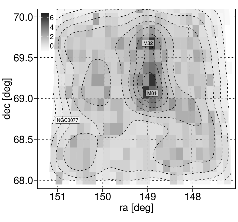
4.2 Colours

The colour-colour diagrams and colour distributions of the candidates provide extra insight into how our method selects the GCs. Figure 10 show 6 representative colour-colour diagrams for the selected sources in the J-PLUS narrow and broad-band filters. The distribution of the sources seem plausible since most of the candidates are within the coverage of the known GCs. However, the candidates with higher proper motions () are overall more spread than their lower proper motion counterparts. To illustrate the foreground extinction and to allow for easy comparison with other GC systems, we show a reddening vector calculated assuming (Schlafly & Finkbeiner 2011) towards the direction of the centre of the field analysed in this work.
In Figure 11 we show narrow and broad-band colour distributions for point sources, spectroscopically confirmed GCs and GC candidates. From the distributions, it is clear that our methodology selects GC candidates roughly consistent with the spectroscopically confirmed GCs in most colours and excludes very red objects (see, e.g. the distributions) that are consistent with background galaxies. In commonly used optical colours such as (Harris et al. 2016) and (Peng et al. 2006, Beasley et al. 2018) our sample of GC candidates peaks at slightly bluer colours, if compared to the spectroscopically confirmed GCs. This goes in hand with what is seen in Figure 9 and is not surprising, given that blue GCs are expected to dominate at large galactocentric radii. Looking at the distribution of candidates, we find that 85 per cent of the low proper motion candidates fall in the range mag, which is in agreement with the typical colours of extragalactic GCs in this photometric system (Sinnott et al. 2010; Chies-Santos et al. 2011a; Faifer et al. 2011; Caso et al. 2019; Ennis et al. 2020, e.g.) under the assumption of foreground reddening mag (Schlafly & Finkbeiner 2011). Moreover, there is a tail of candidates presenting mag, they are mainly fainter than mag and of them have higher proper motion values.

4.3 Metallicities
Based on the sample of 73 spectroscopically confirmed GCs with derived metallicities (Nantais & Huchra 2010), we build a function to map the metallicity distribution of confirmed GCs to their respective photometric bands in order to infer the metallicity distribution function (MDF) of the GC candidates. More specifically, we model the GC metallicity as a function of J-PLUS photometric bands with XGBoost (Chen & Guestrin 2016), a scalable regression-tree-based model that outperforms deep-learning-based approaches when it is comes to model tabular data (Shwartz-Ziv & Armon 2021). In a nutshell, the intuition behind different regression models relies on how we approximate the underlying relationship between a given response variable, here defined by the metallicity, and a set of covariates, herein represented by the first two PCs. The choice for only two PCs is motivated by both being able to explain more than 97 percent of the data variance. In a hypothetical scenario where the relationship could be amenable by a linear regression model, the linear relation would be written as:
| (6) |
Where is the intercept and and are the respective slopes of each covariate. On the other hand, is a preconceived parametric regression does not exists or is unknown, a non-parametric approach is needed. Different solutions have been proposed in the literature, notable examples include additive models, kernel-based models, neural networks and regression-tree models. While a comprehensive discussion about non-parametric regression is beyond the scope of this paper, the underlying intuition behind tree-based models is to approximate the unknown relation by a series of additive functions:
| (7) |
Each corresponds to an independent tree structure , where is a step function and is the - tree. The model then partitions the space of covariates and fits a series of trees in each of them. We choose XGBoost because empirical results have shown that it enables us to uncover complex relations without fine-tuning. Furthermore, we perform a PCA regression instead of using all twelve J-PLUS filters to mitigate co-linearity and over-fitting. Figure 12 displays a pair-wise correlation matrix of the filters and PCs. The filters are highly correlated, a feature known to cause regression models instability. The PCs, on the other hand, show weak to moderate correlation – a desiderata for any regression analysis. Figure 13 displays the correlation between the first two PCs and the J-PLUS filters. The first PC correlates strongly with most of the colours, except for the -band, which is expected since most colours are highly correlated. To convey intuition about the model solution, the left panel of Figure 14 depicts the regression plane between the first two PCs and the [Fe/H] abundance. The colours represent different bins of metallicity. The points depict the metallicities of the training sample, while the contours the predicted value by the XGBoost. The right panel shows the predicted metallicities as open circles and the metallicities of known GCs as solid circles.
In Figure 15 we show the MDF of the GC candidates and the spectroscopically confirmed GCs with metallicities available (including our training sample). We stress that we are using a small and biased training sample, which is far from ideal. Nevertheless, it can give us a grasp of our sample GC candidates’ MDF shape. The top panel of Figure 15 shows that the MDF of the GC candidates is broad, -2.5 [Fe/H] 0.5, but has an important tail towards the metal-rich end (-0.5 [Fe/H] 0.7). A comparison to the work of Caldwell et al. 2011 and the catalogue published in Caldwell & Romanowsky 2016 for the M 31 GC system (bottom panel of Figure 15) shows similarities, including such metal-rich tail at similar values. While the Milky Way GC system shows two clear peaks, this is not seen for either M 31 or the M 81/M 82 systems. A visual inspection of Figure 15 indicates that our method is conservative and does not select GC candidates towards the tails of the MDF of the spectroscopically confirmed GCs. Thus, we caution the reader that we are not complete towards the extremes of metallicity distribution.


4.4 Spectral energy distributions
With the aim of illustrating the shapes of our GC candidate SEDs we show a few example SEDs of GCs of different metallicities and proper motion values in Figure 16. We divide the sample of GC candidates in bins of metallicity, according to the analysis presented in Section. 4.3. From left to right, the panels are divided in bins of metallicity: -1.91 [Fe/H] -1.37; -1.37 [Fe/H] -1.09; -1.09 [Fe/H] -0.76 and [Fe/H] -0.76). From top to bottom we show GC candidates with , and no measured proper motion. A visual inspection suggests that the SEDs resemble significantly the SEDs of confirmed GC (Figure 2), specially the more metal-poor GC candidates (left panels).
5 Summary and Concluding Remarks
To build a large and homogeneous catalogue of GC candidates around the M 81/M 82/NGC 3077 triplet with 12 J-PLUS broad and narrow-bands in 3 pointings, we develop a tailored statistical model. Our model accounts for missing data and small training sets and uses uncertainty aware PCA to flag GC candidates from a sample of point sources, starting from a training set of 73 spectroscopically confirmed GCs that we recover in J-PLUS. GCs are proxies of the formation assemblies of their host galaxies (Brodie & Strader 2006; Beasley 2020) and of their environments (Lee et al. 2010; Huxor et al. 2014; Alamo-Martínez & Blakeslee 2017; De Bórtoli et al. 2022). With the lack of wide-field studies targeting GC systems of spiral galaxies (Kruijssen et al. 2019), such a catalogue is timely. This work showcases the power of principled statistical techniques allied with multi-band surveys in finding extragalactic GCs in and beyond the outskirts of their host galaxy in the local Universe. Our list increases the population of GC candidates around the triplet by 3-fold and provides a testbed for further studies of GC spatial distribution around spirals galaxies.
We study the spatial distribution of the candidate clusters and report an over-density of GC candidates, forming a potential bridge connecting M 81 and M 82. Interestingly, we do not recover a significant population of GC-like objects around NGC 3077, probably due to the fact that the star cluster population of such galaxy is not made of old GCs, but of younger objects, whose SEDs are not part of our training sample. As expected, blue GCs dominate at more considerable distances from M 81 and M 82.
The power of our method is further tested against colour-colour diagrams and colour distributions of the point sources, the confirmed GCs and GC candidates. The bulk of our candidates tends to have bluer colours in typical and colours than the confirmed GCs. Our method generally excludes very red objects, typical of background galaxies. We further map the metallicity distribution of the spectroscopically confirmed GCs into the metallicity distribution of the sample candidates. Furthermore, find that the MDF of GC candidates is in the range of -2.5 [Fe/H] 0.5, but has a tail towards the metal-rich end (-0.5 [Fe/H] 0.7), similar to what is seen in the GC system of M 31 (Caldwell et al. 2011). We present a few SEDs for GC candidates and discuss them in light of what is expected for GC systems.
The method presented here can be straightforwardly applied to other nearby systems in J-PLUS and S-PLUS surveys and more remote systems with the upcoming J-PAS survey. For the specific system studied in this work M 81/M 82/NGC 3077, future developments include follow-up observations of a randomly selected sample of our candidate clusters in order to better quantify the contamination rate, SED fitting to derive stellar population parameters of a cleaner sample of GC candidates and a dedicated study to characterise the properties of the bridge of GCs connecting M 81 and M 82.
Acknowledgements
We thank the anonymous referee for suggestions that improved the paper. ACS acknowledges funding from the Conselho Nacional de Desenvolvimento Científico e Tecnológico (CNPq) and the Rio Grande do Sul Research Foundation (FAPERGS) through grants CNPq-403580/2016-1, CNPq-11153/2018-6, PqG/FAPERGS-17/2551-0001, FAPERGS/CAPES 19/2551-0000696-9, L’Oréal UNESCO ABC Para Mulheres na Ciência and the Chinese Academy of Sciences (CAS) President’s International Fellowship Initiative (PIFI) through grant 2021VMC0005. R.S.S. was supported by the National Natural Science Foundation of China project 1201101284. This work was funded with grants from Consejo Nacional de Investigaciones Científicas y Técnicas de la República Argentina, Agencia Nacional de Promoción Científica y Tecnológica, and Universidad Nacional de La Plata, Argentina. We acknowledge Tamara Civera from the technical member of UPAD for her invaluable work and Alvaro Alvarez-Candal and Juan Antonio Fernández Ontiveros for comments that helped improve the paper. J. V. acknowledges the technical members of the UPAD for their invaluable work: Juan Castillo, Tamara Civera, Javier Hernández, Ángel López, Alberto Moreno, and David Muniesa. R.A.D. acknowledges support from CNPq through BP grant 308105/2018-4, and the Financiadora de Estudos e Projetos – FINEP grants REF. 1217/13 – 01.13.0279.00 and REF 0859/10 – 01.10.0663.00 for hardware support for the J-PLUS project through the National Observatory of Brazil. Based on observations made with the JAST80 telescope at the Observatorio Astrofísico de Javalambre (OAJ), in Teruel, owned, managed, and operated by the Centro de Estudios de Física del Cosmos de Aragón (CEFCA). We acknowledge the OAJ Data Processing and Archiving Unit (UPAD) for reducing and calibrating the OAJ data used in this work. Funding for the J-PLUS Project has been provided by the Governments of Spain and Aragón through the Fondo de Inversiones de Teruel; the Aragón Government through the Research Groups E96, E103, E16_17R, and E16_20R; the Spanish Ministry of Science, Innovation and Universities (MCIU/AEI/FEDER, UE) with grants PGC2018-097585-B-C21 and PGC2018-097585-B-C22; the Spanish Ministry of Economy and Competitiveness (MINECO) under AYA2015-66211-C2-1-P, AYA2015-66211-C2-2, AYA2012-30789, and ICTS-2009-14; and European FEDER funding (FCDD10-4E-867, FCDD13-4E-2685). The Brazilian agencies FINEP, FAPESP, and the National Observatory of Brazil have also contributed to this project.
Data Availability
The raw data underlying this article is available from J-PLUS DR2 http://www.j-plus.es/datareleases/data_release_dr2. The catalogue of GC candidates will be made available at Vizier and https://www.j-plus.es/ancillarydata/dr2_M81_triplet_GC_candidates.
References
- Adebahr et al. (2017) Adebahr B., Krause M., Klein U., Heald G., Dettmar R. J., 2017, A&A, 608, A29
- Ahumada et al. (2020) Ahumada R., et al., 2020, ApJS, 249, 3
- Alabi et al. (2017) Alabi A. B., et al., 2017, MNRAS, 468, 3949
- Alamo-Martínez & Blakeslee (2017) Alamo-Martínez K. A., Blakeslee J. P., 2017, ApJ, 849, 6
- Andreani et al. (2018) Andreani P., Boselli A., Ciesla L., Vio R., Cortese L., Buat V., Miyamoto Y., 2018, A&A, 617, A33
- Austin (2011) Austin P. C., 2011, Multivariate Behavioral Research, 46, 399
- Bassino et al. (2003) Bassino L. P., Cellone S. A., Forte J. C., Dirsch B., 2003, A&A, 399, 489
- Bassino et al. (2006) Bassino L. P., Faifer F. R., Forte J. C., Dirsch B., Richtler T., Geisler D., Schuberth Y., 2006, A&A, 451, 789
- Beasley (2020) Beasley M. A., 2020, Globular Cluster Systems and Galaxy Formation. Springer Nature Switzerland, pp 245–277, doi:10.1007/978-3-030-38509-5_9
- Beasley et al. (2018) Beasley M. A., Trujillo I., Leaman R., Montes M., 2018, Nature, 555, 483
- Bell et al. (2017) Bell E. F., Monachesi A., Harmsen B., de Jong R. S., Bailin J., Radburn-Smith D. J., D’Souza R., Holwerda B. W., 2017, ApJ, 837, L8
- Bertin & Arnouts (1996a) Bertin E., Arnouts S., 1996a, A&AS, 117, 393
- Bertin & Arnouts (1996b) Bertin E., Arnouts S., 1996b, A&AS, 117, 393
- Bica et al. (2015) Bica E., Santiago B., Bonatto C., Garcia-Dias R., Kerber L., Dias B., Barbuy B., Balbinot E., 2015, MNRAS, 453, 3190
- Blakeslee (1999) Blakeslee J. P., 1999, AJ, 118, 1506
- Blakeslee et al. (2012) Blakeslee J. P., Cho H., Peng E. W., Ferrarese L., Jordán A., Martel A. R., 2012, ApJ, 746, 88
- Bressan et al. (2012) Bressan A., Marigo P., Girardi L., Salasnich B., Dal Cero C., Rubele S., Nanni A., 2012, MNRAS, 427, 127
- Brito-Silva et al. (2021) Brito-Silva D., et al., 2021, arXiv e-prints, p. arXiv:2110.04423
- Brodie & Strader (2006) Brodie J. P., Strader J., 2006, ARA&A, 44, 193
- Brodie et al. (2011) Brodie J. P., Romanowsky A. J., Strader J., Forbes D. A., 2011, AJ, 142, 199
- Brüns & Kroupa (2012) Brüns R. C., Kroupa P., 2012, A&A, 547, A65
- Buuren & Groothuis-Oudshoorn (2011) Buuren S. V., Groothuis-Oudshoorn K., 2011, Journal of Statistical Software, Articles, 45, 1
- Buzzo et al. (2022) Buzzo M. L., et al., 2022, MNRAS, 510, 1383
- Caldwell & Romanowsky (2016) Caldwell N., Romanowsky A. J., 2016, VizieR Online Data Catalog, p. J/ApJ/824/42
- Caldwell et al. (2011) Caldwell N., Schiavon R., Morrison H., Rose J. A., Harding P., 2011, AJ, 141, 61
- Caso et al. (2014) Caso J. P., Bassino L. P., Richtler T., Calderón J. P., Smith Castelli A. V., 2014, MNRAS, 442, 891
- Caso et al. (2017) Caso J. P., Bassino L. P., Gómez M., 2017, MNRAS, 470, 3227
- Caso et al. (2019) Caso J. P., Bassino L. P., Richtler T., Salinas R., 2019, MNRAS, 483, 4371
- Cenarro et al. (2014) Cenarro A. J., et al., 2014, in Observatory Operations: Strategies, Processes, and Systems V. p. 91491I, doi:10.1117/12.2055455
- Cenarro et al. (2019) Cenarro A. J., et al., 2019, A&A, 622, A176
- Chen & Guestrin (2016) Chen T., Guestrin C., 2016, in Proceedings of the 22nd ACM SIGKDD International Conference on Knowledge Discovery and Data Mining. KDD ’16. Association for Computing Machinery, New York, NY, USA, p. 785–794, doi:10.1145/2939672.2939785, https://doi.org/10.1145/2939672.2939785
- Chen & de Souza (2022) Chen P., de Souza R. S., 2022, Research Notes of the AAS, 6, 51
- Chies-Santos et al. (2011a) Chies-Santos A. L., Larsen S. S., Wehner E. M., Kuntschner H., Strader J., Brodie J. P., 2011a, A&A, 525, A19
- Chies-Santos et al. (2011b) Chies-Santos A. L., Larsen S. S., Kuntschner H., Anders P., Wehner E. M., Strader J., Brodie J. P., Santos J. F. C., 2011b, A&A, 525, A20
- Chies-Santos et al. (2012) Chies-Santos A. L., Larsen S. S., Cantiello M., Strader J., Kuntschner H., Wehner E. M., Brodie J. P., 2012, A&A, 539, A54
- Choksi & Gnedin (2019) Choksi N., Gnedin O. Y., 2019, MNRAS, 488, 5409
- Choksi et al. (2018) Choksi N., Gnedin O. Y., Li H., 2018, MNRAS, 480, 2343
- Cuevas-Otahola et al. (2021) Cuevas-Otahola B., Mayya Y. D., Puerari I., Rosa-González D., 2021, MNRAS, 500, 4422
- Davidge (2004) Davidge T. J., 2004, AJ, 127, 1460
- De Bórtoli et al. (2022) De Bórtoli B. J., Caso J. P., Ennis A. I., Bassino L. P., 2022, MNRAS, 510, 5725
- De Souza et al. (2014) De Souza R. S., Maio U., Biffi V., Ciardi B., 2014, MNRAS, 440, 240
- Di Tullio Zinn & Zinn (2015a) Di Tullio Zinn G., Zinn R., 2015a, AJ, 149, 139
- Di Tullio Zinn & Zinn (2015b) Di Tullio Zinn G., Zinn R., 2015b, AJ, 149, 139
- Doppel et al. (2021) Doppel J. E., Sales L. V., Navarro J. F., Abadi M. G., Peng E. W., Toloba E., Ramos-Almendares F., 2021, MNRAS, 502, 1661
- El-Badry et al. (2019) El-Badry K., Quataert E., Weisz D. R., Choksi N., Boylan-Kolchin M., 2019, MNRAS, 482, 4528
- Ennis et al. (2020) Ennis A. I., Caso J. P., Bassino L. P., Salinas R., Gómez M., 2020, MNRAS, 499, 2554
- Escudero et al. (2015) Escudero C. G., Faifer F. R., Bassino L. P., Calderón J. P., Caso J. P., 2015, MNRAS, 449, 612
- Evans et al. (2018) Evans D. W., et al., 2018, A&A, 616, A4
- Fabricius et al. (2021) Fabricius C., et al., 2021, A&A, 649, A5
- Fahrion et al. (2020) Fahrion K., et al., 2020, A&A, 637, A27
- Faifer et al. (2011) Faifer F. R., et al., 2011, MNRAS, 416, 155
- Fensch et al. (2020) Fensch J., et al., 2020, A&A, 644, A164
- Fisher & Drory (2008) Fisher D. B., Drory N., 2008, AJ, 136, 773
- Forbes et al. (2011a) Forbes D. A., Spitler L. R., Strader J., Romanowsky A. J., Brodie J. P., Foster C., 2011a, MNRAS, 413, 2943
- Forbes et al. (2011b) Forbes D. A., Spitler L. R., Strader J., Romanowsky A. J., Brodie J. P., Foster C., 2011b, MNRAS, 413, 2943
- Forte et al. (2019) Forte J. C., et al., 2019, MNRAS, 482, 950
- Gaia Collaboration et al. (2016) Gaia Collaboration et al., 2016, A&A, 595, A1
- Gaia Collaboration et al. (2021) Gaia Collaboration et al., 2021, A&A, 649, A1
- González-Lópezlira et al. (2017) González-Lópezlira R. A., et al., 2017, ApJ, 835, 184
- González-Lópezlira et al. (2019) González-Lópezlira R. A., et al., 2019, ApJ, 876, 39
- Harris (1996) Harris W. E., 1996, AJ, 112, 1487
- Harris et al. (2004) Harris J., Calzetti D., Gallagher John S. I., Smith D. A., Conselice C. J., 2004, ApJ, 603, 503
- Harris et al. (2015) Harris W. E., Harris G. L., Hudson M. J., 2015, ApJ, 806, 36
- Harris et al. (2016) Harris W. E., Blakeslee J. P., Whitmore B. C., Gnedin O. Y., Geisler D., Rothberg B., 2016, ApJ, 817, 58
- Harris et al. (2017) Harris W. E., Blakeslee J. P., Harris G. L. H., 2017, ApJ, 836, 67
- Harris et al. (2020) Harris W. E., et al., 2020, ApJ, 890, 105
- Hernitschek et al. (2019) Hernitschek N., et al., 2019, ApJ, 871, 49
- Ho et al. (2007) Ho D., Imai K., King G., Stuart E., 2007, Political Analysis, 15, 199–236
- Hofert et al. (2018) Hofert M., Kojadinovic I., Maechler M., Yan J., 2018, Elements of Copula Modeling with R. Springer Use R! Series, http://www.springer.com/de/book/9783319896342
- Hoff (2007) Hoff P. D., 2007, Ann. Appl. Stat., 1, 265
- Hoff (2018) Hoff P., 2018, sbgcop: Semiparametric Bayesian Gaussian Copula Estimation and Imputation. https://CRAN.R-project.org/package=sbgcop
- Honaker et al. (2011) Honaker J., King G., Blackwell M., 2011, Journal of Statistical Software, 45, 1
- Hudson et al. (2014) Hudson M. J., Harris G. L., Harris W. E., 2014, ApJ, 787, L5
- Huxor et al. (2009) Huxor A., Ferguson A. M. N., Barker M. K., Tanvir N. R., Irwin M. J., Chapman S. C., Ibata R., Lewis G., 2009, ApJ, 698, L77
- Huxor et al. (2014) Huxor A. P., et al., 2014, MNRAS, 442, 2165
- Ishida & de Souza (2011) Ishida E. E. O., de Souza R. S., 2011, A&A, 527, A49
- Ishida & de Souza (2013) Ishida E. E. O., de Souza R. S., 2013, MNRAS, 430, 509
- Ishida et al. (2011) Ishida E. E. O., de Souza R. S., Ferrara A., 2011, MNRAS, 418, 500
- Jang et al. (2012) Jang I. S., Lim S., Park H. S., Lee M. G., 2012, ApJ, 751, L19
- Jolliffe & Cadima (2016) Jolliffe I. T., Cadima J., 2016, Philos. Trans. R. Soc. A Math. Phys. Eng. Sci., 374, 20150202
- Karachentsev & Kudrya (2014) Karachentsev I. D., Kudrya Y. N., 2014, AJ, 148, 50
- Kruijssen et al. (2019) Kruijssen J. M. D., Pfeffer J. L., Reina-Campos M., Crain R. A., Bastian N., 2019, MNRAS, 486, 3180
- Kuhn et al. (2021) Kuhn M. A., de Souza R. S., Krone-Martins A., Castro-Ginard A., Ishida E. E. O., Povich M. S., Hillenbrand L. A., COIN Collaboration 2021, ApJS, 254, 33
- Laevens et al. (2014) Laevens B. P. M., et al., 2014, ApJ, 786, L3
- Larsen (1999) Larsen S. S., 1999, A&AS, 139, 393
- Lee et al. (2010) Lee M. G., Park H. S., Hwang H. S., 2010, Science, 328, 334
- Lee et al. (2019) Lee S.-Y., Chung C., Yoon S.-J., 2019, ApJS, 240, 2
- Li & Gnedin (2019) Li H., Gnedin O. Y., 2019, MNRAS, 486, 4030
- Lim et al. (2013) Lim S., Hwang N., Lee M. G., 2013, ApJ, 766, 20
- Lin et al. (2016) Lin C.-A., Kilbinger M., Pires S., 2016, A&A, 593, A88
- Longobardi et al. (2018) Longobardi A., et al., 2018, ApJ, 864, 36
- López-Sanjuan et al. (2019) López-Sanjuan C., et al., 2019, A&A, 631, A119
- Lupton et al. (2004) Lupton R., Blanton M. R., Fekete G., Hogg D. W., O’Mullane W., Szalay A., Wherry N., 2004, PASP, 116, 133
- Ma et al. (2017) Ma J., et al., 2017, MNRAS, 468, 4513
- Maltby et al. (2018) Maltby D. T., Almaini O., Wild V., Hatch N. A., Hartley W. G., Simpson C., Rowlands K., Socolovsky M., 2018, MNRAS, 480, 381
- Marchi-Lasch et al. (2019) Marchi-Lasch S., et al., 2019, ApJ, 874, 29
- Marín-Franch et al. (2015) Marín-Franch A., Taylor K., Cenarro J., Cristobal-Hornillos D., Moles M., 2015, in IAU General Assembly. p. 2257381
- Mendes de Oliveira et al. (2019) Mendes de Oliveira C., et al., 2019, MNRAS, 489, 241
- Monachesi et al. (2013) Monachesi A., et al., 2013, ApJ, 766, 106
- Nantais & Huchra (2010) Nantais J. B., Huchra J. P., 2010, AJ, 139, 2620
- Nantais et al. (2010) Nantais J. B., Huchra J. P., McLeod B., Strader J., Brodie J. P., 2010, AJ, 139, 1413
- Nantais et al. (2011) Nantais J. B., Huchra J. P., Zezas A., Gazeas K., Strader J., 2011, AJ, 142, 183
- Nelsen (2010) Nelsen R. B., 2010, An Introduction to Copulas. Springer Publishing Company, Incorporated
- Norris et al. (2019) Norris M. A., van de Ven G., Kannappan S. J., Schinnerer E., Leaman R., 2019, MNRAS, 488, 5400
- Oehm et al. (2017) Oehm W., Thies I., Kroupa P., 2017, MNRAS, 467, 273
- Okamoto et al. (2015) Okamoto S., Arimoto N., Ferguson A. M. N., Bernard E. J., Irwin M. J., Yamada Y., Utsumi Y., 2015, ApJ, 809, L1
- Peng et al. (2006) Peng E. W., et al., 2006, ApJ, 639, 95
- Peng et al. (2008) Peng E. W., et al., 2008, ApJ, 681, 197
- Perelmuter et al. (1995) Perelmuter J.-M., Brodie J. P., Huchra J. P., 1995, AJ, 110, 620
- Pota et al. (2013) Pota V., et al., 2013, MNRAS, 428, 389
- Powalka et al. (2017) Powalka M., et al., 2017, ApJ, 844, 104
- R Core Team (2019) R Core Team 2019, R: A Language and Environment for Statistical Computing. R Foundation for Statistical Computing, Vienna, Austria, https://www.R-project.org/
- Reina-Campos et al. (2021) Reina-Campos M., Trujillo-Gomez S., Deason A. J., Kruijssen J. M. D., Pfeffer J. L., Crain R. A., Bastian N., Hughes M. E., 2021, arXiv e-prints, p. arXiv:2106.07652
- Saito et al. (2005) Saito Y., et al., 2005, ApJ, 621, 750
- Santos Barbosa (2020) Santos Barbosa R., 2020, RMLPCA: Maximum Likelihood Principal Component Analysis. https://CRAN.R-project.org/package=RMLPCA
- Sato et al. (2011) Sato M., Ichiki K., Takeuchi T. T., 2011, Phys. Rev. D, 83, 023501
- Schlafly & Finkbeiner (2011) Schlafly E. F., Finkbeiner D. P., 2011, ApJ, 737, 103
- Schuberth et al. (2010) Schuberth Y., Richtler T., Hilker M., Dirsch B., Bassino L. P., Romanowsky A. J., Infante L., 2010, A&A, 513, A52
- Schuberth et al. (2012) Schuberth Y., Richtler T., Hilker M., Salinas R., Dirsch B., Larsen S. S., 2012, A&A, 544, A115
- Sharina et al. (2010) Sharina M. E., Chandar R., Puzia T. H., Goudfrooij P., Davoust E., 2010, MNRAS, 405, 839
- Shwartz-Ziv & Armon (2021) Shwartz-Ziv R., Armon A., 2021, Information Fusion
- Sinnott et al. (2010) Sinnott B., Hou A., Anderson R., Harris W. E., Woodley K. A., 2010, AJ, 140, 2101
- Smercina et al. (2020) Smercina A., et al., 2020, ApJ, 905, 60
- Strader et al. (2005) Strader J., Brodie J. P., Cenarro A. J., Beasley M. A., Forbes D. A., 2005, AJ, 130, 1315
- Tully et al. (2013) Tully R. B., et al., 2013, AJ, 146, 86
- Villaume et al. (2020) Villaume A., Foreman-Mackey D., Romanowsky A. J., Brodie J., Strader J., 2020, ApJ, 900, 95
- Voggel et al. (2020) Voggel K. T., Seth A. C., Sand D. J., Hughes A., Strader J., Crnojevic D., Caldwell N., 2020, ApJ, 899, 140
- Webb & Carlberg (2021) Webb J. J., Carlberg R. G., 2021, MNRAS, 502, 4547
- Wentzell (2009) Wentzell P., 2009, in Brown S. D., Tauler R., Walczak B., eds, , Comprehensive Chemometrics. Elsevier, Oxford, pp 507–558, doi:10.1016/B978-044452701-1.00057-0
- Wentzell & Hou (2012) Wentzell P. D., Hou S., 2012, Journal of Chemometrics, 26, 264
- Wentzell & Lohnes (1999) Wentzell P. D., Lohnes M. T., 1999, Chemometrics and Intelligent Laboratory Systems, 45, 65
- West et al. (1995) West M. J., Cote P., Jones C., Forman W., Marzke R. O., 1995, ApJ, 453, L77
- Wild et al. (2014) Wild V., et al., 2014, MNRAS, 440, 1880
- Yohana et al. (2021) Yohana E., Ma Y.-Z., Li D., Chen X., Dai W.-M., 2021, MNRAS, 504, 5231
- de Blok et al. (2018) de Blok W. J. G., et al., 2018, ApJ, 865, 26
Appendix A Literature sources in the region of the M 81 triplet
In Table 1 we present the previously catalogued 105 confirmed globular clusters from Perelmuter et al. 1995, Nantais & Huchra 2010, Sharina et al. 2010, Jang et al. 2012 and Lim et al. 2013. We detect 95 of these in J-PLUS. However, only 73 are detected in at least 11 of the 12 J-PLUS filters. As outlined in Sect.3, these are the ones used in our statistical analysis. The other 22 are either detected in less than 11 filters or do not pass the stellarity 0.5 cut, and are marked with □ in the table.
| ID | r | (g-i) | [Fe/H] | ||
| (J2000) | (J2000) | [mag] | [mag] | ||
| Id70349∗ | 09 53 03.2 | 69 13 47.4 | 19.818 | 0.880 | -2.41 |
| JM81GC-2‡ | 09 53 20.2 | 69 39 16.4 | 17.751 | 0.983 | -2.30 |
| JM81GC-1‡ | 09 53 26.2 | 69 31 17.5 | 18.559 | 0.916 | – |
| Is90103∗ | 09 53 39.8 | 68 48 00.7 | 17.958 | 0.552 | -2.20 |
| □Id70319∗ | 09 53 42.9 | 69 13 23.9 | 20.357 | 1.328 | -2.31 |
| Is80172∗ | 09 53 51.7 | 68 57 04.4 | 18.682 | 1.069 | -0.77 |
| Nan-4§ | 09 54 04.9 | 69 09 18.8 | 19.550 | 1.532 | +1.10 |
| Id50357∗ | 09 54 11.2 | 69 02 06.6 | 19.199 | 1.262 | -3.62 |
| Is50394∗ | 09 54 16.5 | 69 02 34.4 | 19.017 | 0.804 | -1.50 |
| Is51027∗ | 09 54 20.0 | 69 09 11.1 | 19.151 | 0.630 | -2.47 |
| □Nan-16§ | 09 54 25.1 | 69 08 04.1 | 19.876 | 1.380 | -0.72 |
| Nan-28§ | 09 54 35.7 | 69 06 43.3 | 18.736 | 1.112 | – |
| Nan-31§ | 09 54 38.8 | 69 04 10.5 | 19.125 | 1.413 | +0.08 |
| Nan-32§ | 09 54 39.7 | 69 03 26.8 | 19.685 | 1.087 | -1.51 |
| □Nan-45§ | 09 54 46.5 | 69 10 54.3 | 20.333 | 1.087 | -1.63 |
| □Nan-51§ | 09 54 50.3 | 69 05 08.7 | 20.448 | 0.857 | -2.10 |
| Nan-55§ | 09 54 51.1 | 69 07 50.5 | 19.705 | 1.387 | -0.43 |
| Nan-71§ | 09 54 56.1 | 69 02 31.4 | 19.323 | 1.195 | -0.64 |
| Nan-79§ | 09 54 58.5 | 69 08 08.8 | 20.335 | 1.483 | -0.44 |
| Is50286∗ | 09 54 58.9 | 69 00 58.2 | – | – | -0.04 |
| Id50826∗ | 09 54 58.9 | 69 00 58.2 | 19.885 | 0.470 | -1.46 |
| □Nan-82§ | 09 54 59.8 | 69 09 27.8 | 20.176 | 1.459 | -1.04 |
| Nan-90§ | 09 55 02.2 | 69 05 38.1 | 17.866 | 1.037 | – |
| Nan-96§ | 09 55 02.8 | 69 07 29.8 | 19.352 | 1.198 | -0.29 |
| □Nan-97§ | 09 55 03.3 | 69 02 24.0 | 20.466 | 0.762 | -1.69 |
| Is40165∗ | 09 55 03.8 | 69 15 37.8 | 18.034 | 0.656 | -1.57 |
| Nan-100§ | 09 55 04.4 | 69 05 16.2 | 19.440 | 0.939 | -1.17 |
| Is50037∗ | 09 55 06.4 | 68 56 26.0 | – | – | -2.34 |
| Nan-109§ | 09 55 07.3 | 69 07 34.6 | 20.472 | 1.380 | +1.15 |
| □Nan-114§ | 09 55 08.4 | 69 04 11.5 | 19.975 | 1.473 | -0.81 |
| Nan-115§ | 09 55 09.0 | 69 05 51.9 | 18.841 | 1.391 | -0.89 |
| Nan-116§ | 09 55 09.1 | 69 04 28.7 | 18.877 | 1.085 | -1.44 |
| Nan-118§ | 09 55 09.8 | 69 04 08.0 | 17.082 | 1.117 | -0.81 |
| Nan-129§ | 09 55 14.3 | 69 02 06.6 | 19.808 | 1.082 | -1.48 |
| □Nan-130§ | 09 55 15.2 | 69 00 26.1 | 19.657 | 1.038 | -0.57 |
| Nan-131§ | 09 55 15.3 | 69 05 24.5 | 19.446 | 1.192 | -0.79 |
| Nan-136§ | 09 55 15.6 | 69 05 48.2 | 19.684 | 1.129 | -0.54 |
| Nan-145§ | 09 55 19.2 | 69 05 50.5 | 19.143 | 1.365 | -0.37 |
| □Nan-153§ | 09 55 20.2 | 69 05 38.0 | 20.614 | 1.641 | -0.99 |
| Nan-158§ | 09 55 21.4 | 69 05 32.1 | 18.583 | 1.057 | – |
| Nan-160§ | 09 55 21.9 | 69 06 38.0 | 16.691 | 1.151 | -0.86 |
| Nan-162§ | 09 55 22.1 | 69 05 19.2 | 17.736 | 1.118 | – |
| Nan-175§ | 09 55 25.2 | 69 07 15.0 | 18.874 | 1.021 | -1.37 |
| Nan-179§ | 09 55 25.7 | 69 01 40.2 | 17.180 | 1.484 | -1.26 |
| Nan-188§ | 09 55 29.1 | 69 00 31.3 | 20.438 | 1.215 | -0.05 |
| Nan-190§ | 09 55 29.7 | 69 05 12.1 | – | – | -0.82 |
| Nan-193§ | 09 55 30.1 | 69 06 06.6 | – | – | – |
| □Nan-194§ | 09 55 30.1 | 69 01 59.8 | 20.227 | 1.019 | – |
| Nan-199§ | 09 55 30.8 | 69 07 39.1 | 17.782 | 1.119 | – |
| Nan-209§ | 09 55 32.9 | 69 06 40.1 | 18.471 | 1.040 | – |
| □Nan-215§ | 09 55 34.4 | 69 06 42.6 | 20.508 | 0.572 | -1.97 |
| Nan-218§ | 09 55 34.9 | 68 58 15.0 | 18.703 | 1.205 | -0.80 |
| □Nan-227§ | 09 55 37.2 | 69 06 35.9 | 18.639 | 1.639 | -1.86 |
| Nan-228§ | 09 55 37.3 | 69 02 07.9 | – | – | -0.15 |
| Nan-231§ | 09 55 37.8 | 68 59 17.9 | 19.822 | 1.425 | -0.40 |
| Nan-232§ | 09 55 37.8 | 69 03 28.2 | – | – | -1.41 |
| Nan-236§ | 09 55 38.5 | 69 06 55.4 | 19.478 | 2.013 | -0.95 |
| Nan-239§ | 09 55 39.4 | 69 05 33.0 | 19.692 | 1.157 | -1.49 |
| Nan-244§ | 09 55 40.0 | 69 02 29.9 | – | – | -0.88 |
| Nan-246§ | 09 55 40.0 | 69 04 10.5 | – | – | -1.77 |
| Nan-247§ | 09 55 40.5 | 69 05 25.1 | 19.394 | 1.517 | -1.38 |
| □Nan-253§ | 09 55 41.9 | 68 55 00.9 | 19.557 | 1.379 | -0.12 |
| Nan-256§ | 09 55 43.4 | 69 03 51.9 | – | – | -0.35 |
| Is40181∗ | 09 55 44.1 | 69 14 11.7 | 18.558 | 1.353 | +0.64 |
| Nan-258§ | 09 55 44.2 | 69 04 24.5 | 19.522 | 1.572 | -1.08 |
| Nan-270§ | 09 55 46.1 | 69 01 26.0 | 19.714 | 0.955 | -0.56 |
| Nan-275§ | 09 55 47.7 | 69 06 25.6 | 18.831 | 1.056 | -1.42 |
| Nan-276§ | 09 55 48.0 | 69 07 28.2 | 20.620 | 0.569 | -1.31 |
| Nan-277§ | 09 55 48.0 | 69 03 52.3 | – | – | -0.40 |
| Nan-279§ | 09 55 48.5 | 69 06 12.4 | 19.637 | 1.119 | -0.22 |
| Lim-523 | 09 55 48.6 | 69 42 58.4 | 18.403 | 0.934 | – |
| Nan-280§ | 09 55 48.8 | 69 05 22.6 | 19.660 | 1.040 | -1.69 |
| Nan-282§ | 09 55 49.2 | 69 01 15.6 | 18.677 | 1.088 | -1.08 |
| Nan-288§ | 09 55 50.2 | 68 58 23 | 19.132 | 0.817 | -1.85 |
| Nan-292§ | 09 55 51.3 | 69 03 23.9 | 18.646 | 0.911 | -1.50 |
| Nan-293§ | 09 55 51.9 | 69 07 39.9 | 18.472 | 1.147 | -0.57 |
| Nan-294§ | 09 55 51.9 | 69 08 19.4 | 18.250 | 1.058 | – |
| □Nan-295§ | 09 55 52.1 | 69 07 10.9 | 19.491 | 1.366 | – |
| Lim-617† | 09 55 53.0 | 69 42 11.9 | 19.737 | 1.448 | – |
| Nan-301§ | 09 55 54.5 | 69 02 52.9 | 18.225 | 1.179 | -0.90 |
| Nan-302§ | 09 55 55.0 | 69 00 56.4 | 18.225 | 1.395 | -0.91 |
| □Nan-304§ | 09 55 55.3 | 69 03 37.8 | 19.444 | 1.405 | +0.12 |
| Nan-307§ | 09 55 55.7 | 69 00 03.5 | 18.899 | 0.965 | – |
| Nan-309§ | 09 55 56.2 | 69 02 28.8 | 20.448 | 0.546 | -1.81 |
| Is60045∗ | 09 55 56.9 | 68 52 13.4 | 18.434 | 0.786 | -1.03 |
| □Nan-315§ | 09 55 57.7 | 69 02 23.5 | 19.005 | 1.229 | – |
| □Nan-330§ | 09 56 03.1 | 69 07 19.9 | 19.378 | 1.430 | -0.37 |
| Nan-337§ | 09 56 05.0 | 69 09 21.7 | 19.301 | 0.995 | -0.61 |
| Nan-340§ | 09 56 05.5 | 69 06 43.4 | 18.907 | 1.013 | – |
| □Nan-353§ | 09 56 08.7 | 69 02 24.8 | 20.090 | 1.154 | -1.10 |
| Nan-354§ | 09 56 08.8 | 69 00 23.8 | 20.671 | 1.096 | -1.94 |
| Nan-365§ | 09 56 14.1 | 69 05 05.7 | 20.588 | 1.055 | -1.26 |
| Nan-367§ | 09 56 14.3 | 69 01 30.2 | 19.946 | 1.064 | -1.63 |
| Nan-377§ | 09 56 17.5 | 68 57 12.3 | 19.614 | 1.065 | -1.22 |
| □Nan-378§ | 09 56 17.8 | 68 59 18.9 | 19.652 | 0.963 | -1.08 |
| Nan-379§ | 09 56 17.8 | 69 03 04.9 | 18.880 | 1.142 | -1.33 |
| Nan-385§ | 09 56 18.9 | 68 59 55.6 | 19.790 | 0.800 | -1.79 |
| Nan-388§ | 09 56 21.1 | 69 02 01.8 | 18.651 | 0.900 | -1.46 |
| Nan-398§ | 09 56 27.5 | 69 01 10.1 | 17.446 | 0.849 | -1.53 |
| Nan-404§ | 09 56 31.7 | 69 03 55.2 | 20.157 | 1.163 | -0.26 |
| □Nan-410§ | 09 56 36.9 | 69 01 46.6 | 19.318 | 1.412 | -0.30 |
| Is40083∗ | 09 56 38.5 | 69 22 50.3 | 18.185 | 0.660 | -1.29 |
| Is50225∗ | 09 56 40.6 | 68 59 52.6 | 18.178 | 0.966 | -0.04 |
| HoIX-4-1038⋄ | 09 57 40.0 | 69 03 25.0 | 19.145 | 0.090 | – |
| Id30244∗ | 09 57 54.9 | 68 49 00.4 | 19.582 | 1.025 | -1.76 |
Appendix B MLPCA
In the following, we show a snippet code to run the algorithm in R and python. The code uses as input a matrix of covariates X, a error matrix Xsd of same dimension, and the desired dimension of the projection, p < rank(X).
Appendix C Spatial Distribution
Having information on proper motions, in Figure 17, we show the spatial distribution for each of the GC candidates category colour-coded by counts of GC within each square bin of 0.15 deg on each side. Despite the compelling evidence of GC bridge between M 81 and M 82, considerably contribution comes from GC without proper motion information. Thus, spectroscopic follow-up will be carried out around the region to confirm the potential bridge hypothesis.
Appendix D Flux excess
Besides the astrometric information used in subsection 2.3, Gaia EDR3 provides photometry in three bands, , and . The first one covers the wavelength range from 330 nm to 1050 nm and results from the profile-fitting of the sources in the astrometric field. The latter ones are integrated over a rectangular aperture from the low-resolution spectra observed with two different prisms, and their joint range of wavelength matches with that of the band, with slightly different transmission curves (Evans et al. 2018). The similarity between these passbands leads to the definition of the flux ratio, , as a proxy of crowded regions. Although the flux ratio from the Gaia passbands, , is assumed as an indication of crowded regions, large values can also represent extended objects. This is particularly relevant in the case of GCs in nearby systems, like the M 82/M 82/NGC 3077 triplet, for which the typical effective radii ( arcsec, from , e.g. Harris 1996, 2010 Edition, and Caso et al. 2014, and the distance assumed in this paper) is comparable to the pixel scale for the Gaia astrometric CCD (Gaia Collaboration et al. 2016). Figure 18 shows the flux excess for GC candidates as a function of the colour with blue squares. The majority of the GC candidates present flux excess close to unity, as expected from point sources (Figure 18 and Fabricius et al. 2021). Still, there are plausible candidates and a few less plausible ones with flux excess larger than 2. In contrast, almost all the flux excess for Galactic stars and background galaxies are below 2. However, we are aware that several confirmed GCs also present flux excess close to unity. This feature cannot be used to unequivocally separate GCs from Galactic stars in our sample (but see Voggel et al. 2020).
Appendix E Comparison with foreground extinction estimates
To independently test the photometric calibration of the catalogue and to estimate the mean extinction of the GCs embedded in the M 81 disk, we assumed the following approach based on the spectroscopic metallicities available in the literature for a fraction of the confirmed GCs (Perelmuter et al. 1995; Nantais & Huchra 2010, e.g.), that belong to our photometric catalogue. For such GCs, we calculated simulated magnitudes in the broad-bands from J-PLUS through the SSPs from the CMD web interface55 5 http://stev.oapd.inaf.it/cgi-bin/cmd_3.1, by means of the PARSEC evolutionary tracks (Bressan et al. 2012) and a Chabrier log-normal initial mass function, and a fiducial age of 10 Gyrs. Then, the absorption is estimated as the difference between the simulated and real magnitudes, considering the absorption coefficients from López-Sanjuan et al. (2019) and we estimate the magnitudes from the difference between observed and expected colours, and the transformations from López-Sanjuan et al. 2019. We note that the procedure is largely uncertain, due to the combination of the errors in the spectroscopic metallicities, the assumption of a fiducial age for all the GCs, systematic effects from the SSPs, and the photometric errors. However, it serves the purpose to estimate a mean . By restricting the sample to GCs at projected distances from the galaxy centre to be larger than 12 arcmin, the mean absorptions from the broad-band colours are around mag. The estimated absorptions for these GCs should be ruled by Galactic foreground extinction, which is settled at mag from Schlafly & Finkbeiner 2011. The GCs at less than 12 arcmin from M 81 centre are typically embedded in its disk, their mean absorption reach mag leading to a mean intrinsic absorption in the disk of M 81 of mag. This is considerably lower than the mean value calculated by Nantais et al. 2011, but it is also an estimation from optical data, and the samples in both analysis are not the same.