, , ,
Keywords: random network, random regular graph, distribution of shortest path lengths, moments, mean, variance
The mean and variance of the distribution of shortest path lengths of random regular graphs
Abstract
The distribution of shortest path lengths (DSPL) of random networks provides useful information on their large scale structure. In the special case of random regular graphs (RRGs), which consist of nodes of degree , the DSPL, denoted by , follows a discrete Gompertz distribution. Using the discrete Laplace transform we derive a closed-form expression for the moment generating function of the DSPL of RRGs. From the moment generating function we obtain closed-form expressions for the mean and variance of the DSPL. More specifically, we find that the mean distance between pairs of distinct nodes is given by , where is the Euler-Mascheroni constant. While the leading term is known, this result includes a novel correction term, which yields very good agreement with the results obtained from direct numerical evaluation of via the tail-sum formula and with the results obtained from computer simulations. However, it does not account for an oscillatory behavior of as a function of or . These oscillations are negligible in sparse networks but detectable in dense networks. We also derive an expression for the variance of the DSPL, which captures the overall dependence of the variance on but does not account for the oscillations. The oscillations are due to the discrete nature of the shell structure around a random node. They reflect the profile of the filling of new shells as is increased. The results for the mean and variance are compared to the corresponding results obtained in other types of random networks. The relation between the mean distance and the diameter is discussed.
1 Introduction
Random networks (or graphs) consist of a set of nodes that are connected by edges in a way that is determined by some random process. They provide a useful conceptual framework for the study of a large variety of systems and processes in science, technology and society [1, 2, 3, 4, 5]. The local structure of a random network can be characterized by the degree distribution and its moments , . In particular, the mean degree provides the expected number of neighbors of a random node, while the variance accounts for the width of the degree distribution.
The large scale structure of a random network is captured by the distribution of shortest path lengths (DSPL), or the distance distribution, between pairs of distinct nodes. Properties of the DSPL, which is denoted by , have been studied in random networks with different degree distributions [6, 7, 8, 10, 9, 11, 12, 13, 14, 18, 19, 15, 16, 17, 20, 21, 22, 24, 23, 25, 26]. It was shown that in random networks whose degree distribution has a finite variance, the mean distance between pairs of distinct nodes scales like [6, 7, 12]. This implies that random networks are small-world networks [27, 28, 29, 30, 31]. Moreover, it was shown that scale-free networks, which exhibit a power-law degree distribution of the form , may be ultrasmall depending on the value of the exponent . In particular, for , where the variance of diverges in the infinite system limit, the mean distance scales like [32, 7, 9]. The variance of the DSPL was also studied. It was shown that the DSPL of random networks is typically a narrow distribution, whose width does not grow as the network size is increased [7].
In the study of the DSPL it is convenient to use the tail distribution , which is the probability that the distance between a random pair of distinct nodes and is larger than . In networks that consist of more than one connected component, the distance between nodes that reside on different network components is . In this case the DSPL is restricted to pairs of nodes that reside on the same connected component [15, 16, 24, 23]. In the analysis below we focus on networks that consist of a single connected component. In this case, the mean distance can be obtained from the tail-sum formula [33]
| (1) |
In configuration model networks the degree of each node is drawn independently from a given degree distribution and the connections are random and uncorrelated [34, 35, 6]. The configuration model generates maximum entropy ensembles in which the degree distribution is fixed [6, 31, 34, 35]. Therefore, the configuration model provides a general and highly powerful platform for the analysis of statistical properties of networks. In configuration model networks, the DSPL is completely determined by the degree distribution and the network size . In particular, in the large network limit the mean distance can be approximated by [6, 29, 30, 31]
| (2) |
where
| (3) |
is the mean of the excess degree distribution of nodes selected via a random edge. The excess degree distribution, given by [36]
| (4) |
is obtained by selecting random edges and choosing randomly one of the two end-nodes of the selected edge. The excess degree of such end-node is obtained by extracting the edge that led to that node, reducing its degree by .
The random regular graph (RRG) is a special case of a configuration model network, in which the degree distribution is a degenerate distribution of the form , namely all the nodes are of the same degree , where . In the special case of an RRG, the second moment of the degree distribution satisfies and the excess degree is . As a result, Eq. (2) is reduced to
| (5) |
Recently, the DSPL of the Erdős-Rényi (ER) network [37, 38, 39] and other configuration model networks was calculated using an approach called the random path approach (RPA), which is based on recursion equations [15, 16, 20]. In general, the recursion equations are iterated step by step and the resulting distribution is evaluated numerically. The DSPL obtained from the recursion equations was found to be in very good agreement with the results obtained from computer simulations for configuration model networks with a broad range of degree distributions [16]. In the special case of random regular graphs (RRGs) of degree , the recursion equations yield a closed-form expression for the DSPL, whose tail distribution takes the form [16]
| (6) |
The distribution shown in Eq. (6) is a discrete form of the Gompertz distribution [40, 41]. Eq. (6) coincides with an earlier calculation of the DSPL of RRGs [8]. The existence of a closed-form expression for opens the way to the derivation of compact formulae for the mean distance and the variance of the DSPL of RRGs. The mean distance provides the typical length scale in the network, as well as its scaling with respect to the network size and the degree . The variance provides the width of the peak in the probability mass function .
In this paper we derive a closed-form expression for the moment generating function of the DSPL of RRGs. The moment generating function is expressed in terms of a discrete Laplace transform. The discrete sum is then evaluated using the Euler-Maclaurin formula that applies for sufficiently large networks. Using the moment generating function we obtain closed-form expressions for the mean distance and for the second moment of the DSPL. Using these results we also obtain, for the first time, a closed form expression for the variance . In previous studies [6, 29, 8, 42] it was found that in the large limit the mean distance can be approximated by Eq. (5). On top of this result, we obtain a novel correction term, which is of order , namely independent of . Since the mean distance is logarithmic in , such correction of order is often not negligible. Taking this correction into account yields a very good agreement with the results obtained from computer simulations. However, it does not account for an apparent oscillatory behavior of as a function of and as a function of . These oscillations are negligible in the sparse-network limit but detectable in the dense-network limit. The closed-form expression obtained for captures the overall dependence of the variance on the degree . However, it does not account for the oscillatory behavior of as a function of , which becomes significant in the dense-network limit. The oscillations of and as a function of and are analyzed and discussed. In particular, it is shown that the oscillations become regular when plotted as a function of , when is kept fixed and is varied. The results for the mean and variance of the DSPL are compared to the corresponding results obtained in other types of random networks. The relation to the diameter is also discussed.
The paper is organized as follows. In Sec. 2 we describe the random regular graph. In Sec. 3 we review the calculation of the distribution of shortest path lengths. In Sec. 4 we derive a closed-form expression for the moment generating function of the DSPL. In Sec. 5 we calculate the mean distance . In Sec. 6 we calculate the variance of the DSPL. The results are discussed in Sec. 7 and summarized in Sec. 8.
2 The random regular graph
The RRG is a special case of a configuration model network, in which the degree distribution is a degenerate distribution of the form , namely all the nodes are of the same degree . Here we focus on the case of , in which for a sufficiently large value of the RRG consists of a single connected component [34, 35, 43]. RRGs of any finite size exhibit a local tree-like structure, while at larger scales there is a broad spectrum of cycle lengths. In that sense RRGs differ from Cayley trees, which maintain their tree structure by reducing the most peripheral nodes to leaf nodes of degree . They also differ from Bethe lattices which exhibit a tree structure of an infinite size.
The neighborhood of a given node can be described by a shell structure, in which the first shell consists of the neighbors of and the second shell consists of the neighbors of the nodes of the first shell, which are at distance from . In general, the th shell around consists of all the nodes that are at a distance from [13, 14]. In the infinite network limit, the th shell around each node consists of nodes.
A convenient way to construct an RRG of size and degree ( must be an even number) is to prepare the nodes such that each node is connected to half edges or stubs [3, 44]. At each step of the construction, one connects a pair of random stubs that belong to two different nodes and that are not already connected, forming an edge between them. This procedure is repeated until all the stubs are exhausted. The process may get stuck before completion in case that all the remaining stubs belong to the same node or to pairs of nodes that are already connected. In such case one needs to perform some random reconnections in order to complete the construction.
3 The distribution of shortest path lengths
Consider an RRG consisting of nodes of degree . The distance between a pair of nodes and is given by the length of the shortest path between and . The tail distribution of shortest path lengths between pairs of random nodes is denoted by . In computer simulations this distribution is obtained by generating a large number of network instances from an ensemble of RRGs of a given size and degree . In each network instance one repeatedly selects pairs of random nodes, finds the shortest paths between them and measures their lengths. These results yield the distribution .
Another useful way to sample nodes is via a random edge. In this case one selects a random edge and picks randomly one of the end-nodes of the selected edge. The edge is then deleted, giving rise to a reduced network that includes all the nodes and edges, apart from , also called the cavity graph [45]. The tail distribution of shortest path lengths between pairs of distinct nodes consisting of a node , selected via a random edge , and a random node , on the reduced network from which is removed, is denoted by .
Apart from the tail distributions and , it is also useful to consider various conditional distributions. Consider a pair of random nodes and , such that the distance between them is known to be larger than . The conditional probability provides the probability that the length of the shortest path between and is larger than , given that it is larger than . Similarly, for a pair of nodes consisting of a node , which is selected via a random edge , and a random node , the conditional probability is the probability that the distance between and is larger than , given that it is larger than , in the reduced network from which is removed.
Below we evaluate the conditional probability , namely the probability that the shortest path length between a pair of random nodes and is larger than , given that it is larger than , using the RPA [15, 16, 20]. Since each node in the network (e.g. node ) has neighbors, the boundary condition at is given by
| (7) |
For the conditional probability can be expressed in the form
| (8) |
where is the conditional distribution of shortest path lengths between a node selected via a random edge and a random node in the reduced network in which the edge is removed. The conditional distribution can be further expressed in the form
| (9) |
where the power of reflects the fact that in the reduced network the node is of degree . In general, the conditional distribution is given by
| (10) |
where . This cascade of recursion equations eventually leads to , which can be evaluated directly and is given by
| (11) |
For sufficiently large and for , Eq. (11) can be replaced by
| (12) |
| (13) |
| (14) |
Finally, for we obtain
| (15) |
Similarly, the conditional distribution is given by
| (16) |
The tail distribution is obtained from
| (17) |
| (18) |
Carrying out the summation, we obtain
| (19) |
where
| (20) |
and
| (21) |
The tail distribution , given by Eq. (19), is a discrete version of the Gompertz distribution [40, 41]. It is in agreement with the DSPL of RRGs obtained in Ref. [8].
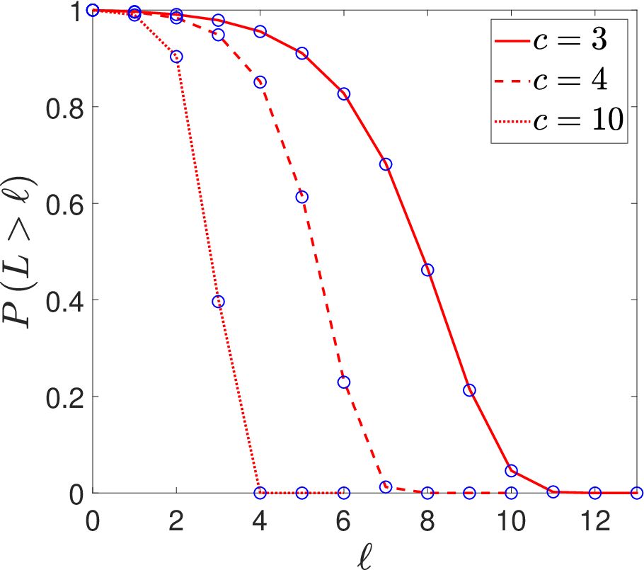
In Fig. 1 we present analytical results for the tail distribution of shortest path lengths for ensembles of RRGs of size and degrees (solid line), (dashed line) and (dotted line). The analytical results, obtained from Eqs. (19)-(21), are in very good agreement with the results obtained from computer simulations (circles). The tail distribution, which follows a discrete Gompertz distribution, exhibits a monotonically decreasing sigmoid-like shape, or a smoothed Heaviside step function. As is increased, the sigmoid function shifts to the left, which implies that distances in the network become shorter. The sigmoid function also becomes steeper, which implies that the DSPL becomes narrower. This means that for sufficiently large values of the majority of pairs of nodes are at equal distance from each other.
The probability mass function of the DSPL can be recovered from the tail distribution by
| (22) |
As mentioned in the introduction, it reflects the shell structure around a random node , where the th shell consists of the nodes that reside at a distance from . The expected number of nodes in the th shell is given by
| (23) |
The Gompertz distribution frequently appears in the analysis of life spans and survival. It describes situations in which the mortality rate grows exponentially with time. The shell structure around a random node can be interpreted in terms of survival probabilities. To explain this property we express Eq. (17) in the form
| (24) |
This implies that the probability of a random node to remain outside the first shells is given by the probability to be outside the first shells times a survival probability, which is given by Eq. (15). The complementary probability is the probability that such random node ends up in the th shell. In the context of survival analysis this probability corresponds to the hazard function or the mortality rate.
4 The moment generating function of the DSPL
In this section we apply a systematic method for the calculation of moments of the DSPL, which is based on the discrete Laplace transform of the tail distribution . The discrete Laplace transform of some function is given by
| (25) |
which is related to the one-sided Z-transform and to the starred transform [46]. Inserting we obtain
| (26) |
where the summation is truncated above . This reflects the fact that in a network that consists of nodes, for . In spite of this fact, note that Eq. (19) yields non-zero results for the probabilities even for . However, these probabilities are vanishingly small. Therefore, the upper limit of the sum in Eq. (26) can be changed from to without affecting the results. We also note that the tail distribution is defined as the distribution of distances between pairs of distinct nodes. Thus, it satisfies . Using these observations, Eq. (26) can be written in the form
| (27) |
The sum on the right hand side of Eq. (27) can be approximated by the corresponding integral. However, a more accurate result can be obtained using the Euler-Maclaurin formula, in which the difference between the sum and the integral is systematically approximated in terms of derivatives of the integrand, which are evaluated at the end-points of the interval [47, 48]. Applying the Euler-Maclaurin formula (equation 2.10.1 in Ref. [49]), we obtain
| (28) | |||||
where is the Bernoulli number of order [49]. Carrying out the integration, we obtain
| (29) |
where is the generalized exponential integral (Eq. 8.19.3 in Ref. [49]). In order to evaluate the sum in Eq. (28), we expand the summand up to first order in . Inserting from Eq. (19), we obtain
| (30) |
where . Expanding Eq. (30) in powers of , we obtain
| (31) | |||||
Differentiating Eq. (31) times with respect to and evaluating the result at , we obtain
| (32) | |||||
Inserting the right hand side of Eq. (32) into Eq. (28) and using the identity (Eq. 4.19.6 in Ref. [49])
| (33) |
we obtain
| (34) | |||||
In the large network limit Eq. (34) can be reduced to
| (35) | |||||
The moment generating function of the DSPL is denoted by
| (36) |
| (37) |
Using Eq. (26) we express the moment generating function in terms of the Laplace transform, namely
| (38) |
In the sections below we use the moment generating function to obtain closed form expressions for the mean and variance of the DSPL.
5 The mean distance
The mean distance between pairs of distinct nodes in an RRG can be calculated using the tail-sum formula [33]
| (39) |
where is given by Eq. (19). Since Eq. (19) is highly accurate for , Eq. (39) is expected to yield accurate results for the mean distance except for the limit of very dense networks. However, this expression provides little insight on the behavior of and its dependence on and . Since , given by Eq. (19), is vanishingly small for , Eq. (39) can be replaced by
| (40) |
Below we use the moment generating function to obtain a closed-form expression for , which is valid for sufficiently large networks. It is given by
| (41) |
| (42) | |||||
where is the exponential integral, also denoted as [49]. Expanding the right hand side of Eq. (42) in powers of , we obtain
| (43) | |||||
where is the Euler-Mascheroni constant [49, 50]. For sufficiently large values of , the corrections of orders and can be neglected, leading to
| (44) |
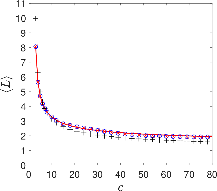
In Fig. 2 we present analytical results (solid line) for the mean distance between pairs of nodes in an RRG of size as a function of the degree , obtained from the closed-form (CF) expression of Eq. (44). We also present the results ( symbols) obtained from a direct numerical evaluation (DE) of the sum in Eq. (40), where is taken from Eq. (19). Since the discrete Gompertz distribution provides highly accurate results for the DSPL, the results obtained from the direct numerical evaluation of Eq. (40) are expected to be accurate. Indeed, they are found to be in very good agreement with the results obtained from computer simulations (circles). The analytical results obtained from Eq. (44) are in very good agreement with the results obtained from direct evaluation and computer simulations. The widely known result of , given by Eq. (5), is also shown ( symbols), indicating that the subleading correction presented in Eq. (44) is important. However, close inspection of Fig. 2 reveals that on top of the overall trend, the mean distance exhibits an oscillatory behavior as a function of , which is not captured by Eq. (44). The amplitude of these oscillations is negligible in the sparse-network limit and becomes detectable for dense networks. Moreover, the period of the oscillations increases as is increased.
Interestingly, in the dense-network limit the direct numerical evaluation of the mean distance can be done using an approximate form of the tail-sum formula of Eq. (40). It is given by
| (45) |
where
| (46) |
and is the integer part of . The first term on the right hand side of Eq. (45) accounts for the sum over the probabilities for , which in the dense-network limit can be approximated by . The next three terms account for the range of distances in which the tail distribution decreases sharply. In the dense-network limit this range is narrow, while the probabilities for are negligible.
To analyze the oscillations, it is convenient to consider the difference , where is the mean distance obtained from direct numerical evaluation of the mean of the discrete Gompertz distribution by Eq. (40), while is the mean distance obtained from the closed-form expression of Eq. (44).
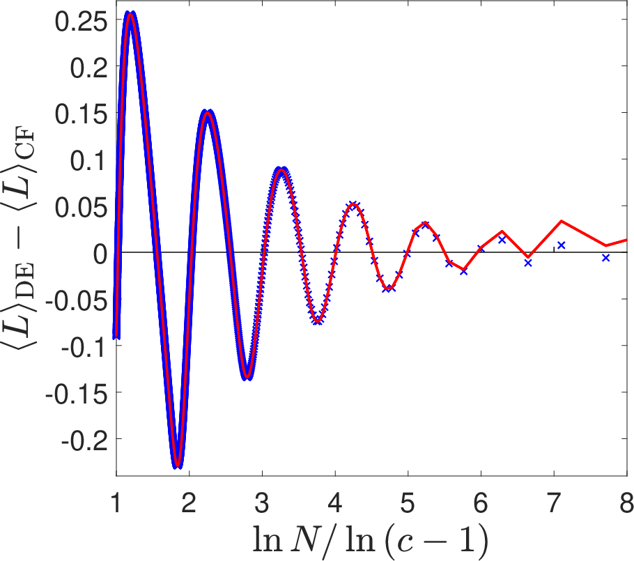
In Fig. 3 we present ( symbols) the difference as a function of where the network size is fixed at and the mean degree is varied. The mean distance is obtained from Eq. (40) and is obtained from Eq. (44). It is found that this difference exhibits oscillations as a function of , whose wavelength is equal to . The amplitude of the oscillations decreases as is increased. The difference vanishes at integer and half-integer values of . It is found that the maxima of the oscillations take place when the fractional part of is approximately , while the minima take place when the fractional part is approximately . We also present approximated results (solid line) in which is evaluated using Eq. (45). The two curves are found to be in very good agreement except for the limit of sparse networks in which Eq. (45) is not expected to provide accurate results. It is important to note that the amplitude of the oscillations is very small compared to the mean distance . Thus, Eq. (44) provides a very good approximation for .
In Fig. 4 we present ( symbols) the difference as a function of , where the degree is fixed at and the network size is varied. The mean distance is obtained from Eq. (40) and is obtained from Eq. (44). It is found that this difference exhibits oscillations as a function of , whose wavelength is equal to . For sufficiently large values of the amplitude of the oscillations is a constant. The difference vanishes at integer and half-integer values of . It is found that the maxima of the oscillations take place when the fractional part of is approximately , while the minima take place when the fractional part is approximately . We also present approximated results (solid line) in which is evaluated using Eq. (45). The two curves are found to be in very good agreement.
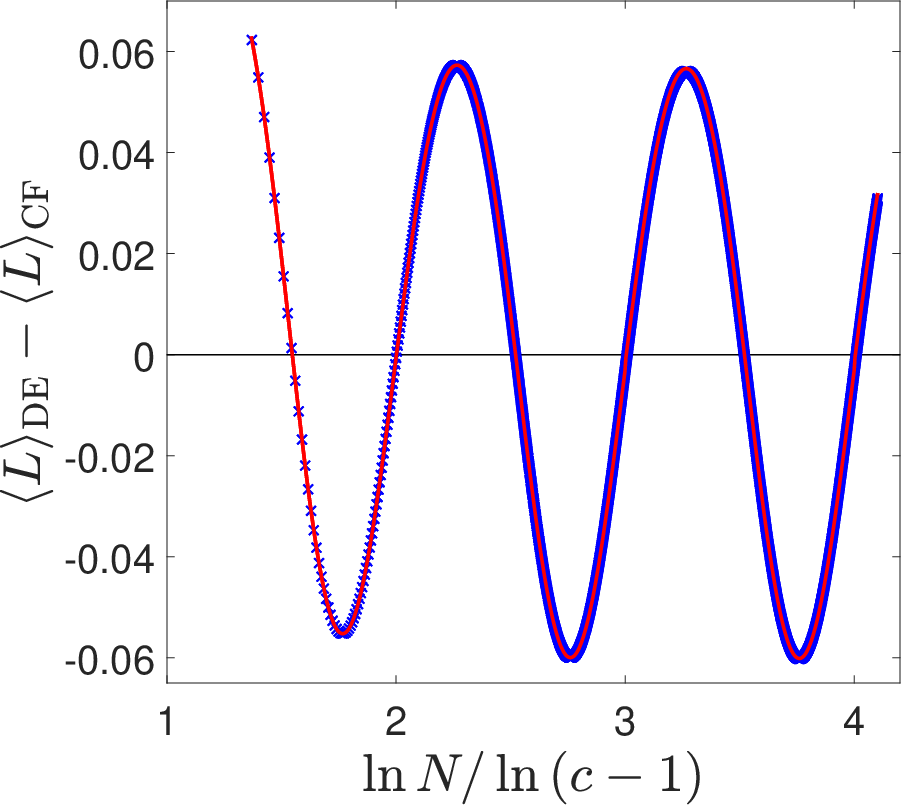
The oscillatory behavior presented in Fig. 4 and specifically the fact that the wavelength is and the amplitude is constant, implies that the difference depends on only via the fractional part
| (47) |
which can be considered as a phase and takes values in the range . Below we show that for sufficiently large this can be rigorously justified. In the large limit, where , Eq. (19) can be reduced to
| (48) |
which can also be written in the form
| (49) |
Using this expression, one can show that
| (50) |
This implies that the dependence of on the network size is only via the phase .
The mean distance can be expressed by
| (51) |
which is justified because for . Shifting the summation variable by to the left, we obtain the equivalent expression
| (52) |
Summing up separately the two terms on the right hand side, we obtain
| (53) |
Expressing the probability in terms of the tail distribution, we obtain
| (54) |
| (55) | |||||
Inserting the probabilities from Eq. (50) into Eq. (55), one finds that is only a function of the degree and the phase . This implies that its dependence on the network size is only via the phase . Note that the argument above holds when the network size is sufficiently large, such that Eq. (50) is a good approximation for Eq. (19).
6 The variance of the DSPL
Using the tail-sum formula, the second moment of the DSPL can be expressed in the form [33]
| (56) |
Since the probability , given by Eq. (19), is vanishingly small for , the upper limit of the summation can be changed from to , without any noticeable change in the result. Therefore,
| (57) |
The variance of the DSPL is given by
| (58) |
Inserting from Eq. (40) and inserting from Eq. (57) into Eq. (58) yields highly accurate results for the variance of the DSPL. However, this expression provides little insight on the behavior of the variance and its dependence on and .
Below we use the moment generating function to obtain a closed-form expression for , which is valid for large networks. It is given by
| (59) |
| (63) | |||||
where is the exponential integral and is the generalized hypergeometric function [49]. Performing an asymptotic expansion for large , we obtain
| (64) | |||||
To obtain the variance of the DSPL we insert from Eq. (63) and from Eq. (42) into Eq. (58). While this result is expected to be relatively precise the resulting expression is complicated. A simpler expression for the variance can be obtained by inserting from Eq. (64) and from Eq. (44) into Eq. (58). In this case the resulting expression can be simplified to the form
| (65) |
This result implies that except for the limit of very small networks, the variance does not depend on the network size but only on the degree . Moreover is a monotonically decreasing function of , whose largest value, obtained at is . We thus conclude that the DSPL of RRGs is a narrow distribution, whose width decreases as is increased.
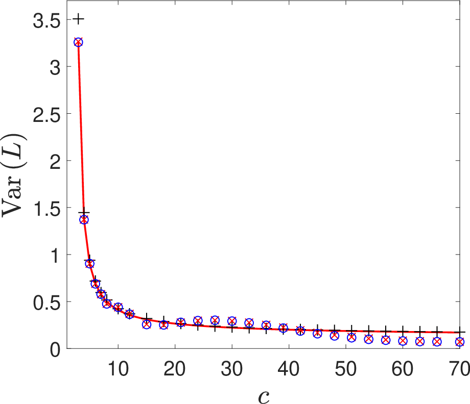
In Fig. 5 we present analytical results (solid line) for the variance for RRGs of size as a function of the degree obtained from Eq. (58), where is given by Eq. (42) and is given by Eq. (63). We also present the results obtained from a direct numerical evaluation ( symbols) of the sums in Eqs. (40) and (57) for and , respectively. These results are found to be in very good agreement with the results obtained from computer simulations (circles). In the regime of sparse networks the analytical results obtained from the closed form expressions of Eqs. (42) and (63) are in very good agreement with the results obtained from direct evaluation and computer simulations. For dense networks the results obtained from direct evaluation and computer simulations exhibit some oscillations that are not captured by the closed form expressions. Instead, the closed-form expressions capture the overall trend of vs. as if the oscillations are averaged out. We also present the results obtained from the simpler expression of Eq. (65) ( symbols). For very small values of , Eq. (65) is found to slightly over-estimate the variance, while for larger values of it is in very good agreement with the results obtained from Eqs. (42) and (63).
In the dense-network limit, the tail sum formula (56) can be approximated by
| (66) |
where is given by Eq. (46). Inserting from Eq. (66) and from Eq. (45) into Eq. (58) and rearranging terms, we obtain
| (67) | |||||
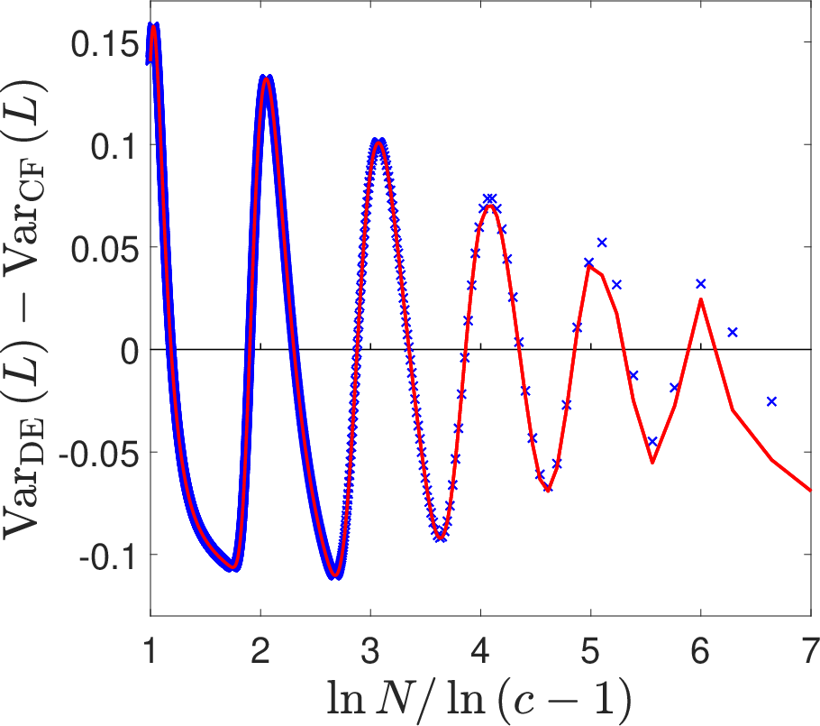
To analyze the discrepancy between the results obtained from the closed-form expressions and those obtained from the direct numerical evaluation of the variance, it is convenient to consider the difference , where is the variance obtained from the direct numerical evaluation of Eqs. (40) and (57) and is the variance obtained from the closed form expressions of Eqs. (42) and (63). It turns out that this difference exhibits oscillations similar to those obtained for , between positive and negative values as a function of . Moreover, the period and the amplitude of these oscillations increase as is increased.
In Fig. 6 we present ( symbols) the difference as a function of for . It is found that this difference exhibits oscillations as a function of , whose wavelength is equal to . The amplitude of the oscillations decreases as is increased. It is found that the maxima of the oscillations take place at integer values of , while the minima take place at half-integer values. This means that around integer values of the closed-form expression provides an under-estimated value for , while around half-integer values of the closed-form expressions provide an over-estimated value for . We also present approximated results (solid line) in which is evaluated using Eq. (67). The two curves are found to be in very good agreement except for the limit of sparse networks in which Eq. (67) is not expected to provide accurate results.
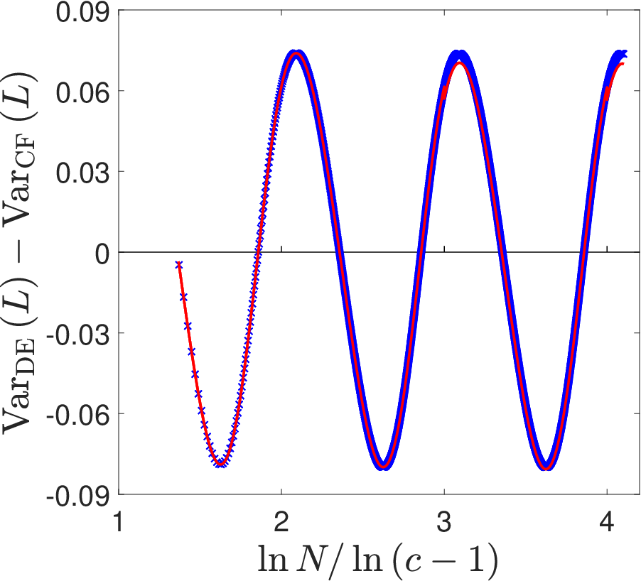
In Fig. 7 we present ( symbols) the difference as a function of where the degree is fixed at and the network size is varied. It is found that this difference exhibits oscillations as a function of , whose wavelength is equal to and the amplitude is a constant. It is found that the maxima of the oscillations take place at integer values of , while the minima take place at half-integer values. This means that around integer values of the closed-form expression provides an under-estimated value for , while around half-integer values of the closed-form expressions provide an over-estimated value for . We also present approximated results (solid line) in which is evaluated using Eq. (67). The two curves are found to be in very good agreement except for the limit of sparse networks in which Eq. (67) is not expected to provide accurate results. The oscillatory behavior presented in Fig. 7 implies that the difference depends on only via the phase . This can be justified using an argument similar to the one presented for the mean distance at the end of Sec. 5.
7 Discussion
In configuration model networks, in the large network limit, the mean distance can be approximated by Eq. (2). It is interesting to compare this result to the corresponding results in models of growing networks. Here we focus on a model of random networks that grow by node duplication (ND), introduced in Ref. [51]. In this model, at each time step a random (mother) node is duplicated. The daughter node is connected to the mother node and is also connected to each one of the neighbors of the mother node with probability . This model exhibits a phase transition at between the sparse-network regime at and the dense-network regime at . In the sparse-network regime, the mean distance is given by [21]
| (68) |
where . Thus, the mean distance of a node duplication network scales logarithmically with as in the case of configuration model networks. However, it was found that for a given network size , the mean distance is significantly larger than the mean distance of a configuration model network with the same degree distribution [21]. The variance of the DSPL of ND networks is given by [21]
| (69) |
Comparing Eqs. (68) and (69), one observes that the mean and variance are the same, which is typical to Poisson-like distributions. This implies that the DSPL of ND networks is a broad distribution whose width scales like . This is in contrast to the case of RRGs, in which the variance is very small and does not scale with the network size.
In directed ND networks not all the pairs of nodes are connected by directed paths. Conditioning on pairs of nodes that are connected by directed paths, it was found that , which is similar to the result for undirected ND networks. However, the variance scales like , which means that the distribution is much broader [22].
Another quantity which is closely related to the mean distance is the mean diameter [52, 53, 54]. Unlike the mean distance which is averaged over all pairs of nodes in each network instance as well as over the ensemble, the mean diameter is averaged only over the ensemble (each network instance provides a single value of the diameter). It was shown that the mean diameter of an ensemble of RRGs is given by [55]
| (70) |
It thus turns out that the expressions for the mean distance and the mean diameter share the same leading term. This is not an obvious result. It appears to reflect the fact that in the shell structure around a random node, most nodes are concentrated in the last few shells. Such networks, in which most of the distances are almost the same, are called idemetric networks [56]. Having said that, the subleading term for the mean diameter scales like , unlike the case of in which it does not depend on . This reflects the fact that the diameter of an RRG of size is the maximal distance between all pairs of nodes. As is increased the number of such pairs increases, making it more probable to find a pair of nodes that are farther away from each other.
8 Summary
The DSPL of RRGs follows a discrete Gompertz distribution. Using the discrete Laplace transform and the Euler-Maclaurin formula we derived a closed-form expression for the moment generating function of the DSPL. From the moment generating function we obtained expressions for the mean distance and for the variance of the DSPL. More specifically, it was found that the mean distance is given by
| (71) |
and the variance of the DSPL is given by
| (72) |
The result for extends known results by adding a correction term, which yields very good agreement with the results obtained from direct numerical evaluation of via the tail-sum formula and with the results obtained from computer simulations. The expression obtained for the variance captures the overall dependence of the variance on the degree . However, it turns out that on top of the overall trend, the mean distance and the variance also exhibit some oscillatory behavior, which is not captured by the closed-form expressions. The oscillations of the mean and variance are due to the discrete nature of the shell structure around a random node. They reflect the profile of the filling of new shells as is increased, or as is decreased. It was shown that these oscillations depend on only via the phase , defined in Eq. (47). This implies regular oscillations with wavelength as a function of , when is varied and is kept fixed. The results for the mean and variance of the DSPL were compared to the corresponding results obtained in other types of random networks. The relation between the mean distance and the diameter was also discussed.
The authors wish to thank one of the anonymous referees for insightful comments and analysis that helped to clarify the nature of the oscillations of the mean and variance of the DSPL. This work was supported by the Israel Science Foundation grant no. 1682/18.
References
References
- [1] Dorogovtsev S N and Mendes J F F 2003 Evolution of Networks: From Biological Nets to the Internet and WWW (Oxford: Oxford University Press)
- [2] Havlin S and Cohen R 2010 Complex Networks: Structure, Robustness and Function (New York: Cambridge University Press)
- [3] Newman M E J 2018 Networks: an Introduction, Second Edition (Oxford: Oxford University Press)
- [4] Estrada E 2011 The Structure of Complex Networks: Theory and Applications (Oxford: Oxford University Press)
- [5] Barrat A, Barthélemy M and Vespignani A 2012 Dynamical Processes on Complex Networks (Boston: Cambridge University Press)
- [6] Newman M E J, Strogatz S H and Watts D J 2001 Random graphs with arbitrary degree distributions and their applications Phys. Rev. E 64 026118
- [7] Dorogovtsev S N, Mendes J F F and Samukhin A N 2003 Metric structure of random networks Nuclear Physics B 653 307
- [8] van der Hofstad R, Hooghiemstra G and Van Mieghem P 2005 Distances in random graphs with finite variance degrees Random Structures & Algorithms 27 76
- [9] van der Hofstad R, Hooghiemstra G and Znamenski D 2007 Distances in Random Graphs with Finite Mean and Infinite Variance Degrees Electronic Journal of Probability 12 703
- [10] Blondel V D, Guillaume J-L, Hendrickx J M and Jungers R M 2007 Distance distribution in random graphs and application to network exploration Phys. Rev. E 76 066101
- [11] van der Hofstad R and Hooghiemstra G 2008 Universality for distances in power-law random graphs J. Math. Phys. 49, 125209
- [12] van der Esker H, van der Hofstad R and Hooghiemstra G 2008 Universality for the distance in finite variance random graphs J. Stat. Phys. 133 169
- [13] Shao J, Buldyrev S V, Cohen R, Kitsak M, Havlin S and Stanley H E 2008 Fractal boundaries of complex networks EPL 84 48004
- [14] Shao J, Buldyrev S V, Braunstein L A, Havlin S and Stanley H E 2009 Structure of shells in complex networks Phys. Rev. E 80 036105
- [15] Katzav E, Nitzan M, ben-Avraham D, Krapivsky P L, Kühn R, Ross N and Biham O 2015 Analytical results for the distribution of shortest path lengths in random networks EPL 111 26006
- [16] Nitzan M, Katzav E, Kühn R and Biham O 2016 Distance distribution in configuration-model networks Phys. Rev. E 93 062309
- [17] Melnik S and Gleeson J P 2016 Simple and accurate analytical calculation of shortest path lengths arXiv:1604.05521
- [18] Goldental A, Vardi R, Sardi S, Sabo P and Kanter I 2015 Broadband macroscopic cortical oscillations emerge from intrinsic neuronal response failures Frontiers of Neural Circuits 9 65
- [19] Goldental A, Uzan H, Sardi S and Kanter I 2017 Oscillations in networks of networks stem from adaptive nodes with memory Scientific Reports 7 2700
- [20] Bonneau H, Hassid A, Biham O, Kühn R and Katzav E 2017 Distribution of shortest cycle lengths in random networks Phys. Rev. E 96 062307
- [21] Steinbock C, Biham O and Katzav E 2017 Distribution of shortest path lengths in a class of node duplication network models Phys. Rev. E 96 032301
- [22] Steinbock C, Biham O and Katzav E 2019 Analytical results for the distribution of shortest path lengths in directed random networks that grow by node duplication Eur. Phys. J. B 92 130
- [23] Tishby I, Biham O, Katzav E and Kühn R 2018 Revealing the microstructure of the giant component in random graph ensembles Phys. Rev. E 97, 042318
- [24] Katzav E, Biham O and Hartmann A 2018 Metric properties of subcritical Erdős-Rényi networks, Phys. Rev. E 98, 012301
- [25] Asher E, Sanhedrai H, Panduranga N K, Cohen R and Havlin S 2020 Distance distribution in extreme modular networks, Phys. Rev. E 101 022313
- [26] Jackson A D and Patil S P 2021 Phases of Small Worlds: A Mean Field Formulation arXiv:2103.14001
- [27] Travers J and Milgram S 1969 An experimental study of the small world problem Socimetry 32 425
- [28] Watts D J and Strogatz S H 1998 Collective dynamics of ‘small-world’ networks Nature 393 440
- [29] Chung F and Lu L 2002 The average distances in random graphs with given expected degrees Proc. Nat. Acad. Sci. USA 99 15879
- [30] Chung F and Lu L 2003 The average distance in a random graph with given expected degrees, Internet Mathematics 1 91
- [31] Fronczak A Fronczak P, and Holyst, J A 2004 Average path length in random networks Phys. Rev. E 70 056110
- [32] Cohen R and Havlin S 2003 Scale-free networks are ultrasmall Phys. Rev. Lett. 90 058701
- [33] Pitman J 1993 Probability (New York: Springer-Verlag)
- [34] Molloy M and Reed A 1995 A critical point for random graphs with a given degree sequence Random Structures & Algorithms 6 161
- [35] Molloy M and Reed A 1998 The Size of the Giant Component of a Random Graph with a Given Degree Sequence Combinatorics, Probability & Computing 7 295
- [36] Newman M E J and Park J 2003 Why social networks are different from other types of networks Phys. Rev. E 68 036122
- [37] Erdős P and Rényi A 1959 On random graphs I Publicationes Mathematicae 6, 290
- [38] Erdős P and Rényi A 1960 On the evolution of random graphs Publ. Math. Inst. Hung. Acad. Sci. 5 17
- [39] Erdős P and Rényi A 1961 On the evolution of random graphs II Bull. Inst. Int. Stat. 38 343
- [40] Gompertz B 1825 On the nature of the function expressive of the law of human mortality and on a new mode of determining the value of life contingencies Philosophical Trans. R. Soc. London A 115 513
- [41] Shklovskii B I 2005 A simple derivation of the Gompertz law for human mortality Theory in Biosciences 123 431
- [42] Shimizu N 2020 The average distance and the diameter of dense random regular graphs The Electronic Journal of Combinatorics 27 P3.62
- [43] Bollobas B 2001 Random Graphs, Second Edition (London: Academic Press)
- [44] Coolen A C C, Annibale A and Roberts E 2017 Generating Random Networks and Graphs (Oxford: Oxford University Press)
- [45] Mézard M and Parisi G 2003 The Cavity Method at Zero Temperature J. Stat. Phys. 111 1
- [46] Phillips C L, Nagle H T, and Chakrabortty A 2015 Digital Control System: Analysis and Design, Fourth Edition (Harlow: Pearson Education)
- [47] Apostol T M 1999 An Elementary View of Euler’s Summation Formula The American Mathematical Monthly 106 409
- [48] Bender C M and Orzag S A 1999 Advanced Mathematical Methods for Scientists and Engineers: Asymptotic Methods and Perturbation Theory (New York: Springer-Verlag)
- [49] Olver F W J, Lozier D M, Boisvert R R and Clark C W 2010 NIST Handbook of Mathematical Functions (Cambridge: Cambridge University Press)
- [50] Finch S R 2003 Mathematical Constants (Cambridge: Cambridge University Press)
- [51] Lambiotte R, Krapivsky P L, Bhat U and Redner S 2016 Structural Transitions in Densifying Networks Phys. Rev. Lett. 117 218301
- [52] Fernholz D and Ramachandran V 2007 The diameter of sparse random graphs Random Structures & Algorithms 31 482
- [53] Riordan O and Wormald N 2010 The diameter of sparse random graphs Combinatorics, Probability & Computing 19 835
- [54] Chung F and Lu L 2001 The diameter of sparse random graphs Advances in Applied Mathematics 26 257
- [55] Bollobás B and de la Vega W F 1982 The diameter of random regular graphs Combinatorica 2 125
- [56] Barmpalias G, Huang N, Lewis-Pye A, Li A, Li X, Pan Y and Roughgarden T 2019 The idemetric property: when most distances are (almost) the same Proc. R. Soc. A 475 20180283