Deep Recurrent Modelling of Granger Causality with Latent Confounding
Abstract
Inferring causal relationships in observational time series data is an important task when interventions cannot be performed. Granger causality is a popular framework to infer potential causal mechanisms between different time series. The original definition of Granger causality is restricted to linear processes and leads to spurious conclusions in the presence of a latent confounder. In this work, we harness the expressive power of recurrent neural networks and propose a deep learning-based approach to model non-linear Granger causality by directly accounting for latent confounders. Our approach leverages multiple recurrent neural networks to parameterise predictive distributions and we propose the novel use of a dual-decoder setup to conduct the Granger tests. We demonstrate the model performance on non-linear stochastic time series for which the latent confounder influences the cause and effect with different time lags; results show the effectiveness of our model compared to existing benchmarks.
Keywords:
latent confounders , recurrent neural networks , time series prediction1 INTRODUCTION
Identifying causal relationships from time series data is important as it helps to facilitate informed decision making. When controlled experiments are feasible, interventions are often performed to break the symmetry of association and provide the direction of causal mechanisms [Eichler 2012], e.g. predicting patients’ response to certain treatments over time [Bica et al. 2020]. In reality, causal inference through interventions is not always feasible as it could be unethical, costly, or simply impossible to carry out, as in the case of financial time series [Hiemstra & Jones 1994] and climate variables [Stips et al. 2016]; in those scenarios we resort to causal inference from observational data.
Granger causality [Granger 1969] is a commonly used framework to infer potential causal relationships. The notion of Granger causality relies on two fundamental principles: 1. the cause precedes the effect in time and 2. the cause contains unique information about the effect not available elsewhere [Eichler 2012]. We say that one time series Granger causes another if its past helps to predict the future values of the target time series [Granger 1969]. Traditionally, model-based Granger causality has been tested mostly on linear dynamics in the form of a vector autoregressive model (VAR) [Yuan & Shou 2020], where one regresses the lagged values of potential causes against the future value of the target series and assess whether the coefficients are statistically different from zero.
Since real world temporal dynamics are rarely linear, several adaptations to model nonlinear causal relationships have been made using for example polynomial autoregression models [Bezruchko et al. 2008] and kernel-based methods [Marinazzo et al. 2011]. Model-free approaches such as transfer entropy [Vicente et al. 2011] are able to detect nonlinear dependencies between time series, however they suffer from high variance and require large amounts of data for reliable estimation [Tank et al. 2021]. In this work, we follow a recent trend that uses neural networks to infer complex nonlinear causal dependencies in time series data [Khanna & Tan 2020, Nauta et al. 2019, Tank et al. 2021, Bussmann et al. 2020, Trifunov et al. 2019, De Brouwer et al. 2020, Marcinkevičs & Vogt 2021, Moraffah et al. 2021].
An important consideration for causal inference from observational time series is confounding bias. A confounder variable affects both cause and effect and therefore must be accounted for to avoid spurious conclusions. Granger causality relies on the causal sufficiency (no latent confounding) assumption [Spirtes & Zhang 2016] and is known to be biased in the presence of confounding [Peters et al. 2017]. Consider the case where the confounder affects the cause variable with lag 2 and the effect variable with lag 4, assuming causal sufficiency would lead to the biased conclusion that Granger causes . When all confounders are observed, one could apply multivariate conditional Granger causality tests [Chen et al. 2006], which relies on the fact that all variables that could have had a possible influence have been considered in the analysis [Marinazzo et al. 2011]. In reality, it is rarely possible to measure all the confounders, nevertheless, we may have access to noisy measurements of proxies for the confounders [Louizos et al. 2017, Pearl 2010]. Since the majority of existing works on neural network-based approaches to Granger causality assume causal sufficiency, how best to account for latent confounders is still an open question. In this work, we use recurrent neural networks (RNN) to infer representations of the latent confounder from the available proxies, which we then use in the subsequent Granger causality tests.
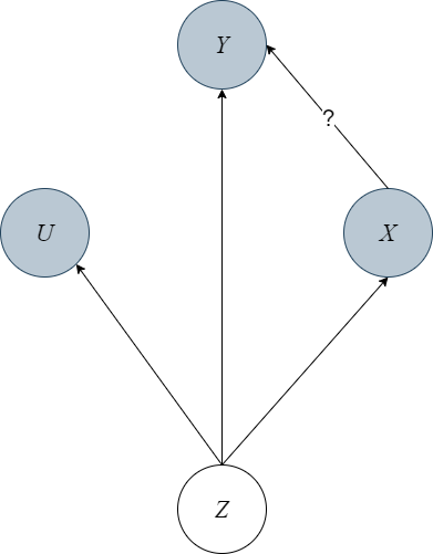
We consider the causal system in Fig. 1 involving a cause variable , an effect variable , a latent confounder and proxies of the confounder , where is the length of the time series and is the number of proxies available. Our aim is infer the Granger causal relationship between the confounded pair and . The main contributions of our work are as follows:
- 1.
we propose a deep learning-based test for nonlinear Granger causality with latent confounding. We leverage the expressive power of recurrent neural networks to infer representations of the latent confounder from the proxy variables and parameterise two predictive distributions for the target variable (with and without ). We apply a two-sample t-test to establish whether the inclusion of results in a statistically significant reduction in prediction error, and hence a Granger causal relationship.
- 2.
we propose the novel use of a dual-decoder setup corresponding to the two predictive distributions mentioned above. This avoids the need to train two separate neural networks for comparison of predictive accuracy
- 3.
we demonstrate the effectiveness of our model on datasets with known data generating processes and we perform a range of sensitivity analyses to show the robustness of our proposed approach
2 RELATED WORK
The original definition of Granger causality [Granger 1969] involves linear dynamics studied using a VAR model. For a collection of time series and a VAR model is defined:
| (1) |
where is the maximum lag considered, is a matrix of coefficients and is a noise term with zero mean. In the linear regime, time series does not Granger-cause series i if for all . Tank et al. 2021 generalise the definition of Granger causality for nonlinear autoregressive models:
| (2) |
where denotes the history of time series and is a nonlinear function mapping the lagged values of other time series to series . Granger non-causality is concluded between series and if for all and all , , implying that does not depend on.
In Tank et al. 2021 the function is parameterised by a multilayer perceptron (MLP) regularised by group lasso penalties and trained with proximal gradient descent to shrink the input weights of lagged values of non-causal time series to zero. Bussmann et al. 2020 propose a neural additive VAR model with each time series expressed as a sum of nonlinear functions of the other time series. The nonlinear functions are parameterised by MLPs and the additive structure allows the contribution of each time series to be analysed separately.
Nauta et al. 2019 propose an attention based convolutional neural network with an explicit validation phase. The attention mechanism learns which time series are attended to during prediction, and interventions on potential causal time series are performed in the validation phase. Khanna & Tan 2020 infer Granger causal relations from a structured sparse estimate of internal parameters of statistical recurrent units [Oliva et al. 2017] trained for time series prediction.
A popular class of methods involves training two neural network time series prediction models and comparing their performances. One model would accept the past values of the target and exogenous variables as inputs, and the other accepts only the past target values. A statistically significant reduction in prediction error is a sign of Granger causality. In existing literature, these prediction models are often different variants of RNNs [Wang et al. 2018, Duggento et al. 2019, Abbasvandi & Nasrabadi 2019] or MLPs [Orjuela-Canon et al. 2020]. Our proposed approach falls within this class of methods however we argue that training two separate neural networks is inefficient and spurious conclusions could be reached due to differences in neural network hyperparameters. In our architecture, we propose to train a neural network with two decoders to alleviate these issues.
With the exception of Nauta et al. 2019, all above-mentioned literature assumes causal sufficiency. How best to account for an unobserved confounder in Granger causal analysis is an open question. In Nauta et al. 2019, the model can only detect a latent confounder if it affects cause and effect with equal time lags. In our work however we consider a more challenging scenario involving different lags in the causal mechanisms. We follow a popular approach involving the use of neural networks to infer representations of the latent confounder (a substitute confounder). Louizos et al. 2017 propose a variational autoencoder to recover the joint distribution of the observed and latent variables which they use to estimate the average treatment effect (ATE) in a static setting. Trifunov et al. 2019 adapt the architecture in Louizos et al. 2017 to a time series setting for the estimation of ATE. Bica et al. 2020 propose a recurrent neural network architecture to build a factor model and estimate ATE using the inferred substitute confounders.
Outside of the deep learning domain, different methods can accommodate hidden confounders to different extents. Chu & Glymour 2008 propose additive nonlinear time series model (ANLTSM) which can only deal with hidden confounders that are linear and instantaneous. Conditional independence based approaches LPCMCI [Gerhardus & Runge 2020] and SVARFCI[Malinsky & Spirtes 2018] detect hidden confounders by inferring a special edge type in the partial ancestral graph.
3 METHODOLOGY
Our proposed approach involves the use of multiple recurrent neural networks to parameterise predictive distributions. We define the full model predictive distribution as . The restricted model distribution is defined as . Parameterising the two predictive distributions allows us to compare the predictive performances of two time series prediction models and a statistically significant reduction in prediction error from the restricted model to the full model is a sign of Granger causality.
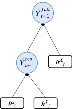
To parameterise the full-model and restricted-model distributions, we leverage the expressive power of recurrent neural networks. In our model we use gated recurrent units (GRU) [Cho et al. 2014]. The architecture of the restricted model is given in Fig. 2. Each GRU is characterised by a sequence of hidden states which contains information of time series up to time . We propose to learn representations of the latent confounder using the available proxies by parameterising the filtering distribution:
| (3) |
The inferred representation of follows an isotropic Gaussian distribution:
| (4) |
where the covariance matrix is diagonal. The dimension of is a tunable hyperparameter. The parameters of the filtering distribution are given by
| (5) |
where is a function approximated by an MLP. To ensure positivity of the standard deviation we use a softplus activation function on the MLP output.

To avoid the need to train two separate time series prediction models, we propose the use of a dual-decoder setup. The restricted-model distribution is normal and given as
| (6) |
The full-model distribution is also normal and expressed as
| (7) |
where is the predicted value of from the restricted model and and are two MLP models. The proposed dual-decoder setup is shown in Fig. 3 and . A combination of Fig.2 and Fig.3 represents the full architecture of the model where the output of the restricted-model serves as one of the inputs of the full-model.
For model optimisation we maximise the following objective function:
| (8) |
where the first and second terms correspond to the full and restricted model distributions respectively, and and are the model parameters to be optimised.
To infer the Granger causal relationship between and in the presence of a latent confounder, we wish to check whether the inclusion of in the full-model results in a statistically significant reduction in prediction error compared to the restricted model. With substitute confounders we perform a two-sample t-test to establish whether (where denotes independence); in such cases we conclude that Granger-causes , and vice versa. We use the mean-squared-error as the error metric.
4 EXPERIMENTS
We first demonstrate the model performance on two arbitrary synthetic datasets with known data generating processes. The nonlinear functions and noise levels have been set arbitrarily. The data generating processes for the two datasets are given by (9) and (10) respectively. We generate 1000 samples and use 800 for training, 100 for validation and 100 for testing.
4.1 Dataset 1
| (9) | ||||
where the hyperbolic tangent and sigmoid functions are used to introduce non-linearity into the system. The noise term is Gaussian of the form .
4.2 Dataset 2
The data generating processes for , and remain the same as in (9). We generate using:
| (10) | ||||
4.3 River discharge dataset
To investigate the model performance on real-world time series, we use the river discharge dataset provided in Gerhardus & Runge 2020. This dataset describes the average daily discharges of rivers in the upper Danube basin. We consider measurements from the Iller at Kempten as , the Danube at Dillingen as , and the Isar at Lenggries as the proxy variable. All three variables are potentially confounded by rainfall or other weather conditions [Gerhardus & Runge 2020]. The Iller discharges into the Danube within a day, implying an instantaneous causal link . For the scope of Granger causality considered in this paper, the cause is required to precede the effect in time [Eichler 2012] so we do not take into account instantaneous causal relationships. We therefore expect no Granger-causal relationship between and . The dataset contains roughly 1000 entries, we use 80% for training, 10% for validation and 10% for testing.
4.4 Neural network parameters
The GRU hidden states , and have a dimension of 5, has a dimension of 1 for the synthetic datasets and 2 for the river discharge dataset, the MLPs , and given in (5,6,7) respectively contain 1 hidden layer with 5 units for the synthetic datasets and 10 units for river discharge, a dropout rate of 0.3 and ReLU activation functions are chosen. We use the ADAM optimiser with a learning rate of 0.001. The sequence length used for model training is 20 with a batch size of 10. These parameters were selected using the validation set through random search.
4.5 Statistical testing
By comparing the sample prediction errors of the full and restricted models, we are able to infer whether a Granger causal relationship between and exists. A two-sample t-test could be used as an additional verification step. For dataset 1&2 (Granger) we adopt the following null and alternative hypothesis:
| (11) | ||||
where and are the mean prediction errors generated by the full and restricted models respectively. For dataset 1&2 (no Granger) we adopt the following alternative hypothesis:
| (12) |
The alternative hypothesis is chosen by comparing the sample mean prediction errors computed by the full and restricted models, I.e. we choose the alternative hypothesis in (11) if the mean sample error of the full model is less than that of the restricted model, and vice versa. In cases where the mean sample errors of the two models differ significantly from one another, the statistical test is perhaps redundant. To perform the two-sample t-test, we generate prediction samples from the restricted and full models and we choose a significance level of .
5 RESULTS & DISCUSSION
In Table 1 we provide the prediction errors of the full and restricted models, the p values of the two-sample t-tests and the Granger causal relationship between and inferred by our model, as well as those inferred by LPCMCI [Gerhardus & Runge 2020] with , maximum lag and 4 preliminary iterations, and SVAR-FCI [Malinsky & Spirtes 2018] with and . These are conditional independence based methods for inferring potential causal relationships and are capable of handling latent confounders.
| Dataset | Restricted-model error () | Full-model error () | p value | Ours | LPCMCI | SVAR-FCI |
|---|---|---|---|---|---|---|
| dataset 1 (Granger) | ✓ | ✓ | ✓ | |||
| dataset 1 (no Granger) | ✓ | ✓ | ||||
| dataset 2 (Granger) | ✓ | |||||
| dataset 2 (no Granger) | ||||||
| river discharge |
We observe from Table 1 that the for all the statistical tests. For dataset 1&2 (no Granger) and the river discharge dataset, we reject the null hypothesis that the mean prediction errors of the restricted and full models are equal and conclude that the inclusion of to predict future values of results in a higher prediction error and therefore does not Granger-cause . For dataset 1&2 (Granger) we reject the null hypothesis and conclude that the inclusion of reduces the prediction errors of and therefore Granger-causes . Our model correctly identifies the correct Granger-causal relationship in all scenarios, whereas LPCMCI and SVAR-FCI identify spurious relationships for dataset 1 (no Granger) and dataset 2 (Granger).
Real-world time series can be highly nonlinear and have different noise levels. We have shown that our model is able to identify the Granger-causal relationship for various nonlinear functions and arbitrary noise levels. We investigate the robustness of our model by varying the signal-to-noise ratio defined as:
| (13) |
where denotes the magnitude of the signal ( without the noise term) at and is the standard deviation of the noise term in the data generating process. For dataset 1&2 (Granger) we wish to find the critical below which the noise term becomes dominant and the model fails to identify the Granger-causal link between and ; to do this we vary the standard deviation of the noise term in (9) and (10). We start with a rough range of to and we use a bisection search strategy to find the critical value . A denotes Granger causality inferred by our model. Results are shown in Table 2. For dataset 1 (Granger) we see that the critical value is approximately 59.22 (highlighted in bold), i.e. the Granger-causal link between and for this set of stochastic time series can only be identified if ; for dataset 2(Granger) .
Lastly, we tested the sensitivity of the model output to the sequence length used in training for dataset 1&2 (Granger). We noted that all , which suggests that our model is able to consistently identify the Granger-causal link given short and long used in training. This is desirable as it indicates that model results are not very sensitive to the choice of hyperparameters.
| Dataset 1 (Granger) | Dataset 2 (Granger) | ||
| 10.00 | 1.00 | 10.00 | 1.00 |
| 55.00 | 21.25 | ||
| 57.81 | 26.88 | ||
| 58.51 | 27.58 | ||
| 59.22 | 28.28 | ||
| 60.63 | 29.69 | ||
| 66.25 | 32.50 | ||
| 77.50 | 55.00 | ||
| 100 | 100 |
6 CONCLUSION
In this paper we have presented a deep-learning based approach to model nonlinear Granger-causality with in the presence of a latent confounder. Our model involves the use of multiple recurrent neural networks to parameterise a restricted-model distribution and a full-model distribution . We generate prediction samples from the two distributions and we use a two-sample t-test to establish whether the inclusion of helps to predict future values of given a learned representation of the confounder. To enable efficient comparison, we propose a dual-decoder setup, which avoids the need to train two separate models (as presented in many existing literature), and we believe this helps to reduce bias resulting from neural network hyperparameter tuning. We demonstrate the effectiveness of our model on both synthetic and real-world datasets, and we recognise that a high enough signal-to-noise ratio is required to correctly identify a Granger-causal link.
Acknowledgements
The authors acknowledge Dr Fabio Caccioli and Dr Brooks Paige (both Dept of Computer Science, UCL) for their advice on the project and the manuscript.
References
- Abbasvandi & Nasrabadi [2019] Abbasvandi, Z., & Nasrabadi, A. M. (2019). A self-organized recurrent neural network for estimating the effective connectivity and its application to EEG data. Computers in Biology and Medicine, 110, 93–107. URL: https://doi.org/10.1016/j.compbiomed.2019.05.012. doi:10.1016/j.compbiomed.2019.05.012.
- Bezruchko et al. [2008] Bezruchko, B. P., Ponomarenko, V. I., Prokhorov, M. D., Smirnov, D. A., & Tass, P. A. (2008). Modeling nonlinear oscillatory systems and diagnostics of coupling between them using chaotic time series analysis: applications in neurophysiology. Physics-Uspekhi, 51, 304–310. URL: https://doi.org/10.1070/pu2008v051n03abeh006494. doi:10.1070/pu2008v051n03abeh006494.
- Bica et al. [2020] Bica, I., Alaa, A. M., & Van Der Schaar, M. (2020). Time series deconfounder: Estimating treatment effects over time in the presence of hidden confounders. In 37th International Conference on Machine Learning, ICML 2020 (pp. 861–872). volume PartF16814. arXiv:1902.00450.
- Bussmann et al. [2020] Bussmann, B., Nys, J., & Latré, S. (2020). Neural Additive Vector Autoregression Models for Causal Discovery in Time Series Data. arXiv preprint, . URL: http://arxiv.org/abs/2010.09429. arXiv:2010.09429.
- Chen et al. [2006] Chen, Y., Bressler, S. L., & Ding, M. (2006). Frequency decomposition of conditional Granger causality and application to multivariate neural field potential data. Journal of Neuroscience Methods, 150, 228–237. doi:10.1016/j.jneumeth.2005.06.011. arXiv:0608034.
- Cho et al. [2014] Cho, K., van Merrienboer, B., Bahdanau, D., & Bengio, Y. (2014). On the Properties of Neural Machine Translation: Encoder–Decoder Approaches. In In Eighth Workshop on Syntax, Semantics and Structure in Statistical Translation (SSST-8). doi:10.3115/v1/w14-4012. arXiv:1409.1259.
- Chu & Glymour [2008] Chu, T., & Glymour, C. (2008). Search for additive nonlinear time series causal models. Journal of Machine Learning Research, 9, 967–991.
- De Brouwer et al. [2020] De Brouwer, E., Arany, A., Simm, J., & Moreau, Y. (2020). Inferring Causal Dependencies between Chaotic Dynamical Systems from Sporadic Time Series. In ICML Workshop on the Art of Learning with Missing Values (Artemiss) 2020 Icml.
- Duggento et al. [2019] Duggento, A., Guerrisi, M., & Toschi, N. (2019). Echo State Network models for nonlinear Granger causality. bioRxiv, (pp. 1–7). doi:10.1101/651679.
- Eichler [2012] Eichler, M. (2012). Causal inference in time series analysis. Causality: Wiley Series in Probability and Statistics, (pp. 6–28). doi:10.1002/9781119945710.ch22.
- Gerhardus & Runge [2020] Gerhardus, A., & Runge, J. (2020). High-recall causal discovery for autocorrelated time series with latent confounders. In 34th Conference on Neural Information Processing Systems NeurIPS. URL: http://arxiv.org/abs/2007.01884. arXiv:2007.01884.
- Granger [1969] Granger, C. J. W. (1969). Investigating Causal Relations by Econometric Models and Cross-spectral Methods. Econometrica, 37, 424–438.
- Hiemstra & Jones [1994] Hiemstra, C., & Jones, J. (1994). Testing for linear and nonlinear Granger causality in the stock price-volume relation. The Journal of Finance, 49, 1639–1664.
- Khanna & Tan [2020] Khanna, S., & Tan, V. Y. F. (2020). Economy Statistical Recurrent Units For Inferring Nonlinear Granger Causality. In 8th International Conference on Learning Representations, ICLR 2020. URL: http://arxiv.org/abs/1911.09879. arXiv:1911.09879.
- Louizos et al. [2017] Louizos, C., Shalit, U., Mooij, J., Sontag, D., Zemel, R., & Welling, M. (2017). Causal effect inference with deep latent-variable models. Advances in Neural Information Processing Systems, 2017-December, 6447–6457. arXiv:1705.08821.
- Malinsky & Spirtes [2018] Malinsky, D., & Spirtes, P. (2018). Causal Structure Learning from Multivariate Time Series in Settings with Unmeasured Confounding. In Proceedings of 2018 ACM SIGKDD Workshop on Causal Disocvery 2010 (pp. 1–25).
- Marcinkevičs & Vogt [2021] Marcinkevičs, R., & Vogt, J. E. (2021). Interpretable Models for Granger Causality Using Self-explaining Neural Networks. In 9th International Conference on Learning Representations, ICLR 2021. URL: http://arxiv.org/abs/2101.07600. arXiv:2101.07600.
- Marinazzo et al. [2011] Marinazzo, D., Liao, W., Chen, H., & Stramaglia, S. (2011). Nonlinear connectivity by Granger causality. NeuroImage, 58, 330–338. URL: http://dx.doi.org/10.1016/j.neuroimage.2010.01.099. doi:10.1016/j.neuroimage.2010.01.099.
- Moraffah et al. [2021] Moraffah, R., Sheth, P., Karami, M., Bhattacharya, A., Wang, Q., Tahir, A., Raglin, A., & Liu, H. (2021). Causal Inference for Time series Analysis: Problems, Methods and Evaluation. arXiv preprint, . URL: http://arxiv.org/abs/2102.05829. arXiv:2102.05829.
- Nauta et al. [2019] Nauta, M., Bucur, D., & Seifert, C. (2019). Causal Discovery with Attention-Based Convolutional Neural Networks. Machine Learning and Knowledge Extraction, 1, 312–340. doi:10.3390/make1010019.
- Oliva et al. [2017] Oliva, J. B., Poczos, B., & Schneider, J. (2017). The statistical recurrent unit. In 34th International Conference on Machine Learning, ICML 2017 (pp. 4098–4107). volume 6. arXiv:1703.00381.
- Orjuela-Canon et al. [2020] Orjuela-Canon, A. D., Freund, J. A., Jutinico, A., & Cerquera, A. (2020). Granger Causality Analysis based on Neural Networks Architectures for bivariate cases. Proceedings of the International Joint Conference on Neural Networks, (pp. 1–6). doi:10.1109/IJCNN48605.2020.9206977.
- Pearl [2010] Pearl, J. (2010). On measurement bias in causal inference. Proceedings of the 26th Conference on Uncertainty in Artificial Intelligence, UAI 2010, (pp. 425–432). arXiv:1203.3504.
- Peters et al. [2017] Peters, J., Janzing, D., & Schlkopf, B. (2017). Elements of Causal Inference: Foundations and Learning Algorithms. The MIT Press.
- Spirtes & Zhang [2016] Spirtes, P., & Zhang, K. (2016). Causal discovery and inference: concepts and recent methodological advances. Applied Informatics, 3. doi:10.1186/s40535-016-0018-x.
- Stips et al. [2016] Stips, A., MacIas, D., Coughlan, C., Garcia-Gorriz, E., & Liang, X. S. (2016). On the causal structure between CO2 and global temperature. Scientific Reports, 6, 1–9. doi:10.1038/srep21691.
- Tank et al. [2021] Tank, A., Covert, I., Foti, N., Shojaie, A., & Fox, E. B. (2021). Neural Granger Causality. IEEE Transactions on Pattern Analysis and Machine Intelligence, (pp. 1–14). doi:10.1109/TPAMI.2021.3065601. arXiv:1802.05842.
- Trifunov et al. [2019] Trifunov, V. T., Shadaydeh, M., Runge, J., Eyring, V., Reichstein, M., & Denzler, J. (2019). Nonlinear Causal Link Estimation Under Hidden Confounding with an Application to Time Series Anomaly Detection. In 41st DAGM German Conference on Pattern Recognition, DAGM GCPR 2019 (pp. 261–273). volume 11824 LNCS. doi:10.1007/978-3-030-33676-9_18.
- Vicente et al. [2011] Vicente, R., Wibral, M., Lindner, M., & Pipa, G. (2011). Transfer entropy-a model-free measure of effective connectivity for the neurosciences. Journal of Computational Neuroscience, 30, 45–67. doi:10.1007/s10827-010-0262-3.
- Wang et al. [2018] Wang, Y., Lin, K., Qi, Y., Lian, Q., Feng, S., Wu, Z., & Pan, G. (2018). Estimating brain connectivity with varying-length time lags using a recurrent neural network. IEEE Transactions on Biomedical Engineering, 65, 1953–1963. doi:10.1109/TBME.2018.2842769.
- Yuan & Shou [2020] Yuan, A. E., & Shou, W. (2020). Data-driven causal analysis of observational time series: A synthesis. bioRxiv, . URL: https://doi.org/10.1101/2020.08.03.233692.