A Bayesian Deep Learning Approach to Near-Term Climate Prediction
Abstract
Since model bias and associated initialization shock are serious shortcomings that reduce prediction skill in state-of-the-art decadal climate prediction efforts, we pursue a complementary machine-learning-based approach to climate prediction. The example problem setting we consider consists of predicting natural variability of the North Atlantic sea surface temperature on the interannual timescale in the pre-industrial control simulation of the Community Earth System Model (CESM2). While previous works have considered the use of recurrent networks such as convolutional LSTMs and reservoir computing networks in this and other similar problem settings, we currently focus on the use of feedforward convolutional networks. In particular, we find that a feedforward convolutional network with a Densenet architecture is able to outperform a convolutional LSTM in terms of predictive skill. Next, we go on to consider a probabilistic formulation of the same network based on Stein variational gradient descent and find that in addition to providing useful measures of predictive uncertainty, the probabilistic (Bayesian) version improves on its deterministic counterpart in terms of predictive skill. Finally, we characterize the reliability of the ensemble of ML models obtained in the probilistic setting by using analysis tools developed in the context of ensemble numerical weather prediction.
Computational Science Initiative, Brookhaven National Laboratory, Upton, NY 11973, USA Los Alamos National Laboratory, Los Alamos, NM 87545, USA
keypoints
Model bias and associated initialization shock are serious shortcomings that reduce prediction skill in state-of-the-art decadal climate prediction efforts. A complementary machine-learning-based approach to climate prediction is considered. Both deterministic and probabilistic machine learning approaches are examined. In addition to providing useful measures of predictive uncertainty, Bayesian versions of deep learning models outperform their deterministic counterparts in terms of predictive skill.Plain Language Summary
Businesses and government agencies rely heavily on numerical predictions of climate variables such as temperature and precipitation for a wide variety of purposes ranging from integrated assessment to developing mitigation strategies to developing resilience and adaptation strategies. Developing interannual to decadal predictions using comprehensive and complex climate and earth system models, however, are computationally intensive. As such, computationally efficient and accurate surrogates of comprehensive earth system models is highly desired. Data-driven models using advanced deep learning algorithms are promising for this purpose. This paper first considers a recently proposed convolutional network architecture to develop such a surrogate and then integrates Bayesian inference to this architecture to further assess predictive uncertainty. We show that the resulting Bayesian deep learning model not only improves prediction accuracy but also quantifies the uncertainty arising from the data and model.
1 Introduction
The climate system consists of diverse yet interconnected components, such as the atmosphere, oceans, etc., and each can exhibit complex, multiscale, and chaotic behaviors. Additional interactions and feedbacks among these subsystems drive dynamic evolution over an enormous range of spatial and temporal scales in the climate system IPCC (2007); Stocker et al. (2013); Masson-Delmotte (2021). In this setting, comprehensive climate models have emerged as a powerful tool in helping unravel and better comprehend the myriad processes underlying climate and climate change. Moreover, studies using such models have greatly improved the understanding of climate system processes over the past few decades Masson-Delmotte (2021).
Importantly, comprehensive climate models have helped to better anticipate the climate system’s response to external forcings, such as those stemming from increased greenhouse gases that typically are realized on a timescale of a few decades or longer. At shorter timescales at which natural variability plays an increasingly important role, however, improvements in the ability to predict climate are not commensurate with advances in understanding dynamics and processes IPCC (2007); Stocker et al. (2013); Masson-Delmotte (2021). Notably, improvements in predicting the El Niño-Southern Oscillation (ENSO) remain more of an exception than the rule. Poor predictive skill at the shorter timescales is due to the fact that sources of predictability at these timescales reside in modes of natural variability of the climate system, and because models have difficulty in representing and capturing such modes and their timing with adequate accuracy.
Modes of natural variability in the climate system often are associated with delicate balances between multiple physical processes, and realizing those same balances in a climate model is difficult. This leads to biases in a model’s representation of the modes of variability. These model biases also exist in the representation of the mean climate state. While the downstream dynamical consequences of such model biases tend to be both complicated and manifold, from a dynamical systems perspective, an overall consequence tends to be that the model attractor is biased as well.
One way to understand poor predictive skill at shorter timescales is in terms of bias in the model’s representation of the climate attractor: when initialized predictions attempt to realize the predictability associated with natural variability by initializing the model state to be consistent with an observed climate state, the biased model attractor quickly pulls it away. This leads to the model trajectory exhibiting a jump away from the observed trajectory toward the biased model attractor that typically involves complicated nonlinear dynamics. An invariable effect tends to be loss of predictive skill Nadiga, Verma et al. (2019).
The current approach for dealing with this loss of skill consists of statistically correcting the predictions in a post-processing step. Given the nonlinear and complicated dynamics that take place to effect the dramatic readjustment of the flow field (e.g., Sanchez-Gomez et al. (2016)), namely, the jump-like behavior of the initialized prediction trajectory, it is unlikely that the statistical post-processing of the predictions is capable of correctly compensating for these dynamics.
Given the problems associated with a comprehensive climate-model-based approach to near-term predictions, we are interested in investigating and developing alternative data-driven approaches to such predictions. Herein, we split future climate into “near-term” and “long-term” and define near-term to mean the period over which initial conditions (IC) matter. Thus, while long-term predictability is solely determined by boundary conditions (BC) and/or forcing, near-term predictability is affected by both BC/forcing and IC.
In particular, we are investigating the utility of an approach for predicting near-term variations in a quantity of interest (QoI) that is based on learning spatiotemporal variability of that QoI in a controlled setting. Such learning can be achieved using both feedforward and recurrent neural networks (FNN, RNN respectively) (and transformer networks that are beginning to outperform RNNs in at least certain applications). Using RNNs for learning spatiotemporal variability can be traced back to applying optical flow-based computer vision techniques to extrapolate radar echo images toward nowcasting convective precipitation (e.g., see Sakaino (2012)). Further developments along these lines wherein precipitation nowcasting is formulated in the general framework of a “sequence-to-sequence” learning problem—transforming a sequence of past radar maps to a sequence of future radar maps—quickly led to the proposal of a convolutional long short-term memory (convLSTM) architecture/approach Xingjian et al. (2015). In essence, a convLSTM network determines the future states of a QoI at a spatial location using past states of a local neighborhood and other inputs. Subsequently, convLSTM has emerged as a machine learning (ML) technique that delivers good performance in various applications. This is especially evident in some previous work involving climate-relevant settings of predicting interannual variations of global surface temperature and sea-surface temperature in ocean basins Nadiga, Jiang & Farimani (2019); Park et al. (2019); Jiang et al. (2019). As such, even as other recurrent neural network (RNN) architectures have emerged in the context of sequence-to-sequence learning (e.g., attention-based transformers) and are displacing convLSTM as the state-of-the-art, this work is restricted to considering feedforward architectures and comparing their performance to convLSTM. We will report on ongoing work using attention-based methods elsewhere.
Another contribution of the present work consists of considering the ML-based prediction of near-term climate variations in a probablistic fashion as opposed to a deterministic approach. In the context of numerical weather prediction (NWP), the chaotic nature of atmospheric dynamics necessitates considering the evolution of an ensemble of trajectories in order to make reliable forecasts (of the one trajectory that actually is realized in the observed weather system). Starting with the statistical-dynamical prediction methods of Epstein (1969) and more widely adopted at NWP centers across the globe since the early 1990s11 1 The European Center for Medium-Range Weather Forecasts (ECMWF) has been leading the charge., probabilistic forecasts using an ensemble prediction system (EPS) have proven to be valuable in improving the skill of weather forecasts.
Likewise, we expect that probablistic ML models of spatiotemporal variability of climate will be both more skillful and useful than deterministic ML models. However, probabilistic ML remains in its infancy. As such, developing and applying efficient probabilistic deep learning models is difficult, and studies examining their utility and performance are few. In this context, assuming the network parameters (weights and biases) are random variables and applying Bayes’ rule provide the theoretical basis for inferring the posterior distribution of the network parameters that best fit the training data. Here, we note that (parametric) variational inference (VI) methods were developed to efficiently approximate such inference computationally by minimizing the Kullback-Leibler (KL) divergence between an approximate posterior and the true posterior. Subsequently, to extend the use of VI beyond the specialized families of distributions that enjoy particular conjugacy properties, approaches to nonparametric VI have been developed. Our study considers the Stein variational gradient descent (SVGD) approach to nonparametric VI. By adapting and applying this probablistic deep learning approach to the climate prediction problem being considered, we find that as in the context of NWP, a probabilistic ML approach serves to improve on the skill of a deterministic ML approach.
Next, we comment on the nature of the ensemble in a probabilistic ML setting. For this, it is useful to note that in the NWP setting—a first-principles-based setting—two kinds of ensembles have typically been used in EPSs: (1) Initial condition ensembles (ICE) where the model (is assumed to be perfect and so the model) configuration is held fixed and uncertainty in estimation of the state of the system is represented by an ensemble of initial conditions. (2) Perturbed physics ensembles (PPE) where the initial condition is held fixed, but the parameterizations that are used to represent unresolved processes are perturbed to represent uncertainty related to model error. In the current data-driven probabilistic ML setting, uncertainty represented by the ensemble may be thought of in the PPE sense as the diversity of predictions can be traced back to perturbations of the weights and biases that constitute the model’s parameters. In this data-driven setting, while it is true that the probabilistic learning algorithm is trying to learn generalities over a diverse set of IC to infer the perturbations of the ML model parameters that are required, the IC diversity in the training data is not a representation of uncertainty in state estimation as would be required for an ICE.
Finally, we make novel use of diagnostics developed for NWP-EPS in an ML context. This is motivated by the fact that the goal of ensemble prediction, whether it is in the more traditional context of ensemble prediction systems or in the current probabilistic ML context, is for the prediction to span the range of likely outcomes given the uncertainties Leith (1974). These diagnostics are based on the joint analysis of error and ensemble variance. To the best of our knowledge, we use these diagnostics for the first time in the context of probabilistic ML to gain added insight into both the network architecture and the process of probabilistically inferring the weights of the network. In this context, we note, however, that the joint analysis of error and ensemble variance can be carried out in many ways and we consider only the most elementary/simplest of such methods. Using the error-spread and rank-histogram diagnostics, we find, in a global sense, that the ML prediction ensemble is underdispersed. And the behavior persists on enlarging the size of the ensemble. This leads us to further considering the reliability diagnostics in a spatially localized or fine-grained sense. On so doing, a more complicated picture emerges: There are some regions, such as the subpolar North Atlantic, where the ML ensemble is actually overdispersed. However there are other larger regions, such as equatorial and tropical North Atlantic, where the ensemble is underdispersed. Therefore, in the aggregate an overall underdispersive behavior emerges. As such making changes to the probabilistic ML methodology to further improve the reliability of the prediction ensemble and making it optimally reliable tends to be tricky.
The rest of the paper is organized as follows. Section 2 presents the details of the data and definitions of prediction problem. Section 3 discusses the proposed Bayesian deep learning model, including the key derivation, architecture designs, training and testing procedures, and implementation guidelines. Section 4 performs a comparative study on different models and covers a qualitative and quantitative examination of the climate predictions. Finally, conclusions and suggestions for future developments are provided in section 5.
2 Data and Problem Setup
2.1 Spatiotemporal Variability of Sea Surface Temperature in the North Atlantic
We consider the spatiotemporal variability of sea surface temperature (SST) in the North Atlantic over the last 800 years of the pre-industrial control simulation, or piControl, a simulation in which external forcing is held fixed, from the Community Earth System Model (CESM) Danabasoglu et al. (2020) as part of the sixth phase of the Coupled Model Intercomparison Project (CMIP6). CESM2 is a global coupled ocean-atmosphere-land-land ice model, and the piControl simulation considered herein uses the Community Atmosphere Model (CAM6) and Parallel Ocean Program (POP2) at a nominal 1o horizontal resolution in both the atmosphere and ocean. Readers can refer to Danabasoglu et al. (2020) for details. These data are publicly available from the CMIP archive at https://esgf-node.llnl.gov/projects/cmip6 and its mirrors. These monthly data display variability on a large range of spatial and temporal scales. The largest spatial variation is in the meridional (i.e., latitudinal) direction, while the largest temporal variation is at the annual timescale and represents the seasonal cycle. Because both variations are easily learned and predicted, we preprocess the data to remove these components. The latitudinal variation is eliminated by subtracting the time-mean SST at each geographical location, and the seasonal cycle is removed by considering a 12-month moving average also at each geographical location.
2.2 Formulation of the Learning Problem
Without loss of generality, we cast the near-term climate prediction problem in a video prediction format with the model input-output relationship described by a mapping of the form:
| (1) |
where and denote the respective model input and output, and represent samples of and along the temporal dimension (that are chronologically ordered and at a constant sampling frequency), and SST is considered on a regular latitude (H) and longitude (W) spatial grid. Equivalently, the prediction problem may be written as:
| (2) |
where denotes the current state. Direct prediction of futures states are made given a sequence of past and current states . The schematic in Figure 1 outlines the prediction problem.

3 Methodology
The goal is to develop efficient probabilistic deep learning models for near-term climate prediction while using advanced inference methods in the context of deep neural networks. This section describes our Bayesian learning strategy, the network architectures used, and other specifics regarding the training and testing procedure.
3.1 Bayesian Deep Learning
Estimation and quantification of the various sources of uncertainty is critical to establish the reliability of an ML model and provide an assessment of confidence in its predictions Ghahramani (2015). This aspect of modeling is particularly important in the context of deep learning because of the large number of parameters that have to be leared in the DL setting. To that end, we consider a probabilistic formulation that allows for characterizing uncertainties associated both with the data and model Kendall & Gal (2017).
We assume that the weights have a probability density function of a fully factorized Gaussian prior with zero mean and a precision that is Gamma-distributed. Specifically, Bayesian deep learning (BDL) treats the network parameters as random variables that can be generated via a prior distribution . By constructing the likelihood function from the given training data set , Bayes’ rule can be used to infer the posterior distribution of the network parameters :
| (3) |
Subsequently, the predictive distribution can be obtained by sampling the posterior .
For the regression problem stated in Section 2.2, consider a deterministic neural network , where is the input, is the output and the parameters include both the weights and biases. While deterministic DL models treat the network parameters as deterministic unknowns, BDL considers as random variables to account for epistemic uncertainty induced both by limitations of the model (hypothesis set) considered and limited sampling of the data. A further additive noise term is used to model the irreducible aleatoric uncertainty in the data in this setting leading to
| (4) |
3.1.1 Prior definition
As little is known about the network parameters before training, a non-informative prior typically is suggested to reduce and minimize the bias associated with the introduction of a prior Neal (2012). Assuming that the prior is a fixed distribution independent of the input, we find imposing a sparsity-inducing prior on weights via a hierarchical Bayesian model provides good performance. In particular, epistemic uncertainty of model parameters is described by a fully factorized Gaussian with zero mean and Gamma-distributed precision:
| (5) |
This results in a prior with a Student’s T-distribution centered at zero. By tuning the rate parameter and the shape parameter , one can employ a wider region with heavy tails than a standard Gaussian Luo & Kareem (2020); Zhu & Zabaras (2018). In this study, and are the values taken for the rate and shape parameters. On the other hand, aleatoric uncertainties capturing the noise in the data are assumed to be homoscedastic. Here, we prescribe additive noise same for all output pixels/grids for lower memory and faster computation. Explicitly, the noise term is defined as , where is a scalar denoting the standard deviation of the data and is Gaussian noise, i.e., . In this work, the noise precision is modeled as a random variable with a conjugate prior in the form of
| (6) |
to better simulate the real-world applications. In most applications, the prior noise variance is assumed to be very small, e.g., , so that providing a good initial guess for the prior hyperparameters Gramacy & Lee (2012). Here, we consider the shape and rate parameters to be and . It is worth noting that is a learnable parameter that is derived from data. Consequently, in the posterior estimation step, we will learn model parameters and data parameter . Unless otherwise specified, let denote all the uncertain parameters for brevity.
3.1.2 Posterior estimation
The second step of Bayesian learning is to estimate the posterior with predefined prior distributions. One of the standard ways to obtain the approximate posterior is to use sampling methods Neal (2012). Given a large number of network parameters, e.g., tens or hundreds of millions in a modern deep learning model, this approach can be slow and difficult to converge. In recent years, significant progress has been made using VI methods as an alternative to approximate high-dimensional posterior distributions Blei et al. (2017).
Let be the training data. With a specified prior and a specified functional form for the likelihood, VI casts the Bayesian inference problem as an optimization problem. For a given likelihood and prior , the latter seeks to minimize the KL divergence between a proxy distribution and the posterior distribution :
| (7) |
where is the unnormalized posterior and is the normalizer, also called model evidence. In practice, the normalization constant is not considered in the KL divergence minimization Blei et al. (2017). Also, the proxy distribution is usually parameterized with a specified form of distributions , inevitably introducing deterministic biases Blundell et al. (2015). In this work, SVGD, a nonparametric VI algorithm, is adopted Liu & Wang (2016). Without defining a variational approximation family as parametric VI methods do, SVGD employs a set of independent identically distributed particles and minimizes the KL divergence between the empirical measure of these particles and the true posterior. The central idea is to iteratively move the set of particles toward the true posterior using the gradient descent method:
| (8) |
where is a small number representing the step size in the updating scheme and is the optimal perturbation direction that gives the steepest KL divergence gradient:
| (9) |
with denoting a positive definite kernel. In this work, we choose a standard radial basis function kernel for . In Equation (9), the gradient term pushes the particles toward high-density regions of the target distribution, and the repulsive force term imposes diversity and prevents particle collapse Liu & Wang (2016). Overall, the SVGD updating procedure can be summarized in five steps:
Step 1: compute the joint likelihood .
Step 2: calculate the gradient by back propagation.
Step 3: compute the kernel matrix and its gradient .
Step 4: calculate the kernel Stein operator using equation (9).
Step 5: Update via stochastic gradient descent.
3.1.3 Predictive distribution
On completion of training, the model can be applied to make probabilistic predictions using unseen data samples ; the predictive distribution is given by
| (10) |
Note that the SVGD algorithm provides a sample representation of the posterior . Meaning one can use the learned SVGD particles to estimate the predictive distribution than the direct integration. Furthermore, effectively, the BDL model can be viewed as an ensemble of deep learning models where the number of ensemble members is given by the particle number (e.g., in this work), we can approximate the moments of the predictive distribution using the Monte Carlo method. For instance, the ensemble mean prediction is given by the mean over the particles:
| (11) |
and uncertainties are estimated utilizing the second moment of the predictive distribution:
| (12) |
With the estimated mean and variance, we can make the prediction for new data samples and quantify its associated predictive uncertainty.
3.2 Architecture Design
Even as the success of applying deep learning to problems in science and engineering depends crucially on the choice of network architecture, designing efficient and effective networks remains problem-specific and requires human expertise. In this context, we note climate-relevant data typically are high dimensional, geographically heterogeneous, and most often result from dynamical and other physical interactions over a diverse range of spatial and temporal scales Reichstein et al. (2019).
In regard to the high-dimensional nature of climate data, recent studies reveal that the intrinsic dimension captured by dimensionality reduction techniques tends to be too low and, therefore, insufficient Kashinath et al. (2021). Consequently, rather than rely on dimensionality reduction techniques, we use an architecture that considers the full extent of the spatial degrees of freedom present in the data Xu et al. (2021). Next, motivated by the fact that common yet important fluid-dynamic processes, such as advection and diffusion, are represented by regular stencils in the numerical solution of partial differential solutions governing the climate system, we use convolution layers as an integral aspect of the network. Finally, to permit the learning of multiscale interactions, e.g., both local and remote interactions, we employ a bottleneck of sufficiently high dimension with additional optional fully connected layers in the bottleneck. Notably, this design maintains the deep learning promise of automatically extracting features, allowing them to interact appropriately for the task on hand and subsequently projecting them back at the required resolution in an end-to-end fashion.
In Figure 2, the down- and up-sampling learning modules greatly reduce the number of network parameters, thereby accelerating the training process. Specifically, convolution operations are performed to reduce the data size and extract features. Non-adjacent connections then are established for aggregating extracted features He et al. (2016). As most deep learning models are data-intensive, a densely connected convolutional network structure, known as dense block, is adopted in our encoder-decoder architecture to reduce network parameters and support more stable learning Huang et al. (2017). Consequently, each layer can reuse the features extracted from all preceding layers in the dense block. Inside each dense block, a layer is defined as a set of composition operations usually denoted as convolution, nonlinear activation, batch normalization, and dropout He et al. (2016). We combine image resizing techniques and convolution in the upsampling learning module. In particular, transposed convolutions are commonly performed for upsampling the extracted features to the desired spatial dimensions. However, Odena et al. (2016) find transposed convolutions with uneven overlapping cause a checkerboard pattern of artifacts. Therefore, image resizing techniques, such as nearest-neighbor or bilinear interpolation, serve as good alternatives. For instance, bilinear interpolation discourages high-frequency artifacts via an implicitly weighting filter, which is adopted here. Lastly, we observe pooling operations, usually implemented in-between successive convolution layers to reduce the size of feature maps, can deteriorate prediction performance. Knowing climate data, by nature, differ from most computer science application data (e.g., handwriting digits), we argue that max or average pooling may lead to the loss of distinctive features to infer finer pixel-wise regression. Hence, pooling operations are not considered. Instead, a convolution operator with a non-unit stride is used to manage the feature sizes Dumoulin & Visin (2016).

For the multiscale interactions that typically underlie climate data, a brute force solution consists of a fully connected multilayer perceptron (MLP) model Goodfellow et al. (2016). Thus, the influence from long-distance locations is seamlessly integrated into the MLP architecture. However, an MLP model can be memory-demanding and computationally prohibitive because the number of total parameters increases too quickly, i.e., as the cumulative product of the number of perceptrons in each layer. A better, more efficient way to account for long-distance effects is to add a fully connected linear layer in the feature space, ideally at the bottleneck level. The combination of convolutional and fully connected layers has shown its effectiveness in many computer vision tasks, such as objective detection and image segmentation Dosovitskiy et al. (2020); Rasp et al. (2020). Hence, we also consider fully connected layers between the densely connected encoder and decoder. In such a case, it is anticipated that the fully connected layers will relieve part of the burden on the encoder-decoder parts of the network to learn remote interactions, freeing them to better represent spatiotemporally local interactions—and convolution layers excel at these tasks.
Following such reasoning, we develop our deep learning (DL) model and its Bayesian version (BDL) for climate prediction. We also include the state-of-the-art dynamics forecasting model, ConvLSTM, in the study for better comparison. Here, all three models have a convolutional encoder to condense information. Of note, DL and BDL share the same architecture, and BDL is initialized and stored in a predefined particle number. We defer the network parameter details, including size of the convolving kernel, stride of the convolution, zero-padding size, etc., to A. Figure 2 offers a graphic illustration of the proposed model.
3.3 Network Training
The goal of network training is to minimize the mismatch between a prediction and the correct output . For DL and ConvLSTM, denotes the model output. On the other hand, is defined as the predictive mean of Bayesian particles in BDL. The mean squared error (MSE) is selected as the criterion here to measure the difference between and in each grid. Training details for all models are given as: (1) the data set is split into a training set consisting of paired samples () and a test set containing samples in all experiments; (2) the data is standardized by removing the mean and scaling to unit variance; (3) the batch size of both training and test sets are set the same as for non-probabilistic models and for Bayesian models; (4) the Adam stochastic gradient descent algorithm is used as the default optimizer with weight decay specified to to regularize the weights via an L2 penalty Kingma & Ba (2014), which ensures the model generalizes better to unseen data; (5) the initial learning rate is set to with a dynamic scheduler to reduce the learning rate by a factor of 10 when the computed metric has stopped improving; and (6) the dropout technique is used after each convolutional layer to further reduce overfitting and improve generalization error Hinton et al. (2012), where the probability of an element to be zeroed is set to .
3.4 Implementation Notes
We consider Python 3.7.3 and PyTorch 1.7.0 to implement the methodology. All data processing and model training assessments are carried out on a NVIDIA Tesla V100 graphics processing unit (GPU) card with 16 GB high-bandwidth memory (HBM). For full reproducibility of the results, the computer codes and data can be found at https://xihaier.github.io/ upon publication.
4 Results and Discussions
Figure 3 shows a measure of the magnitude of interannual internal/natural variability that we are interested in predicting. It is computed as the standard deviation of the interannual anomaly of SST. We also refer to this as the climatological standard deviation. This variability is seen to be geographically heterogeneous with the largest variations in the subpolar North Atlantic and the isolated part of the Eastern Pacific (related to ENSO). We nondimensionalize prediction error using the climatological standard deviation to make the errors geographically commensurate and to facilitate comparison of prediction error across different regions.

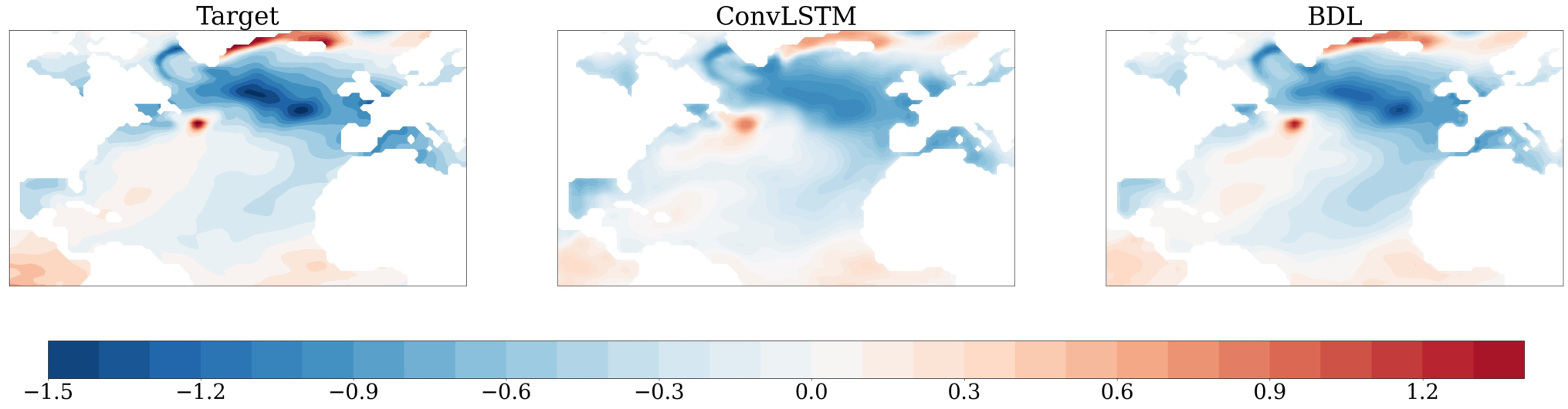
Figure 4 compares the predictions of SST in the North Atlantic at a lead time of six months for a randomly selected test case. The target spatial distribution of SST is shown in the left panel and we recall that both the strong, time-mean latitudinal variability and the seasonal cycle have been removed in the current study so as to focus largely on the interannual component of variability. As such the main variability seen in the target distribution is related to the spatial heterogenity of the nature of interannual variability. On comparing the predictions in the other two panels with the target distribution, it is seen that both the convLSTM prediction (center panel) and the ensemble-mean of the BDL prediction (right panel) successfully capture the main aspects of the spatial distribution such as the warm spot near Grand Banks, the cooler temperatures of the subpolar gyre, the warm anomaly in the East Greenland current, the lower variability in the subtropical gyre region, and others. However, it is also seen that whereas the convLSTM predictions tend to be more diffuse, features in the BDL prediction are better correlated with the target and tend to be sharper even though we are considering an ensemble-average. This is suggestive of better performance of the probablisitic BDL system as compared to the deterministic convLSTM system Xingjian et al. (2015); Park et al. (2019); Xu et al. (2021).
This observation is confirmed on examining the prediction accuracy averaged over the entire test data set of 128 test samples. Figure 5 shows the prediction error pattern map at a lead time of six months for convLSTM and BDL. The error is specifically defined as the non-dimensional root mean square error (NDRMSE), with the climatological standard deviation being used to non-dimensionalize the RMSE at each location. Results at other lead times are qualitatively similar.

Figure 6 compares the prediction error of DL and BDL for the same test sample as shown in Fig. 4, but at a lead time of twelve months. Two features are seen in this comparison: error is seen to be lower in the Bayesian model, and the error in the deterministic model is seen to have smaller scale features. This suggests the possibility that the deterministic DL model is more prone to overfitting and that the averaging inherent in the Bayesian DL acts to regularize the BDL predictions. This, in turn, reiterates the need to assess model and data uncertainty using probabilistic modeling techniques, particularly when considering deep networks Ghahramani (2015).

Figure 7 compares the domain averaged error as a function of prediction lead time in the various models considered. For convLSTM, DL, and BDL, NDRMSE averaged (over the domain and) over the test sets are shown in filled circles. A further fit of the inidividual points using an function of the form , with denoting the prediction lead time is also shown. The fit is obtained by minimizing the residual in a nonlinear least-squares problem using a trust-region algorithm Conn et al. (2000). Along with the previously mentioned models, the damped persistence fit, obtained by fitting a first order autoregressive model is shown and indicated as AR1.

First, it is seen that for the most part, irrespective of whether it is FNNs or RNNs, and whether it is deterministic ML models or probabilistic ones, each of the ML models performs better than damped persistence. Next, it is interesting to note that DL and BDL, both feedforward networks (FNN) outperform the convLSTM model, a recurrent network (RNN) that has previously been seen to provide good performance in a variety of temporal prediction settings. Furthermore, the probabilistic Bayesian deep learning model performs better than its deterministic counterpart, as discussed earlier. Finally, for BDL, uncertainty is estimated as the standard deviation of the ensemble spread and is shown by the red envelope in Figure 7. The uncertainty in prediction is seen to increase with lead time. In an RNN setting, in contrast to the current FNN setting, it is typical to train the recurrent network to produce a one step prediction. Thereafter, predictions at longer lead times are produced based on both the input at the current time and output at the previous time. Thus, compounding of error and uncertainty with increasing lead time explains the increase of both error and uncertainty with increasing lead time in an RNN setting. On the other hand, in the current FNN setting, the straight forward process of compounding of error and uncertainty with increasing lead time is absent and thus constitutes an independent validation of the current FNN approach. Indeed, we go on to consider the nature of these increases with time further in the following section.
In terms of computational cost, our implementation of the DL model (primarily based on convolution operations) is approximately 20 times faster than the ConvLSTM model. We have further verified this speed-up in the contest of a larger data set Park et al. (2019); Xu et al. (2021). It is worth noting that the time complexity of training a Bayesian network is theoretically , where n denotes the number of particles in the SVGD algorithm Liu & Wang (2016). In all experiments, we find that the BDL model achieves better scalability than linear complexity and requires less training time than the ConvLSTM model.
4.1 Quantification and Nature of Uncertainty as Represented in the Bayesian Deep Learning Model
Now that we have a probabilistic prediction system that takes into account the possibility of a range of models fitting the training data in a Bayesian framework, we are able to generate a range of outcomes for the test data as well. Such a distribution of predictions has multiple uses including obtaining information of alternative future evolutions and the possibility of predicting extreme events. However, given the experimental nature of the probablistic prediction system considered, we presently confine ourselves to examining the quality of the predictions and its utility in providing insights into the methodology itself.
In addition to the slight improvement in prediction skill when compared to deterministic deep learning models (DL and ConvLSTM), BDL allows for a means of quantifying the uncertainty inherent in the data and model. For example, in the particular approach we consider, learning the posterior distribution of , a parameter related to data uncertainty and whose prior distribution is given in (6) serves to quantify data uncertainty. Likewise, the learning of the posterior distribution of the model parameters , the priors for which are given in (5) serves to capture uncertainty in the model itself. While we have already shown and briefly discussed the behavior of uncertainty in the BDL in the previous section, we seek to analyze it further in this section and see what further insight it may yield into the workings of the Bayesian model.
The rightmost panel in Figure 8, shows an estimate of uncertainty in the prediction of the SST for a particular instance, defined as the standard deviation of the ensemble. Prediction uncertainty varies depending on the underlying dynamical state and the dynamics underlying SST varies significantly from the tropics to the midlatitude and sub-polar regions. This is reflected in the spatial heterogenity of the uncertainty estimated in the BDL scheme. The heterogenity of the estimated uncertainty is in agreement with the hetrogenity of the magnitude of interannual variability shown in Fig. 3. Finally, the figure also shows that the higher (lower) level of error in the subpolar (tropical) region is accompanied by a higher (lower) level of uncertainty.

We previously saw the growth of uncertainty with increasing prediction lead time in a domain-averaged sense in Fig. 7. Figure 9 shows the spatial distribution of the growth of uncertainty with prediction lead time. The spatial heterogenity is related to the hetrogenity of the dynamics governing the evolution of SST as discussed previously. The higher level of uncertainty in the isolated patch of the Pacific in the southwest corner of the domain is likely due to the fact that the dynamics in that region is controlled more by processes in the rest of the Pacific that is not considered presently.

Next, we focus attention on the nature of the relationship between prediction error and uncertainty. The reason for doing this is because in a realistic situation we do not have verification data. As such, we cannot directly estimate error in (or skill of) the predictions. So, the question is, as to what extent the uncertainty in the prediction can be used as a measure of prediction error? It is somewhat natural to think that the future state will be close to the ensemble mean when the dispersion of the ensemble is small and conversely for the accuracy of the ensemble mean to small when the ensemble is highly dispersed. As such, we proceed to quantify the relationship between ensemble spread and prediction accuracy of BDL when verification data is present.
The inset in the top left panel of Fig. 10 shows a scatterplot of error of the ensemble-mean against ensemble-spread at each geographical location, for each of the test instances, and at each prediction lead time of between one and eighteen months. In this inset plot, a large degree of scatter is seen and error and spread are moderately correlated; the Spearman correlation coefficient is 0.33. (We prefer to use the rank-based Spearman correlation coefficient since a) it is a nonparametric measure of monotonicity of the relationship between the two variables, b) unlike the Pearson correlation, it does not assume that the variables are normally distributed, which makes it more robust.) Here we note that even in idealized experiments where the prediction model is perfect (in the sense that it does not have any biases), for statistical reasons, the spread-error correlation need not be large (e.g., see Barker91, Houtekamer93).
The inset in the bottom-right shows the Spearman correlation coefficient as a function of the prediction lead time. The correlation coefficient is seen to decrease largely monotonically with lead time. The low correlation at long lead time corresponds to the prediction reverting to climatology.

The large scatter in the spread-error plot is due to considering the predictions at the highest level of detail available. Given the usual reduced predictability of the smaller of spatio-temporal scales (equivalenty, increased predictability of the larger of spatiotemporal scales), the question naturally arises as to the nature of this correlation when the predictions are considered in a less-detailed or more-aggregated fashion. To examine this, we consider a bin-averaging strategy: Previously, (e.g., wangbishop2003) binning only along the spread axis, followed by bin-averaging spread and error has been suggested. However, on implementing this procedure, we find that it leads to the predicted error falling in a range that is very narrow compared to the actual range of errors. For this reason, we consider binning along both the spread and error axes. First, the bin-edges for each axis was determined such that each bin contains an equal number of points. Next, the (spread, error) tuples were binned in the sense of a two-dimensional histogram using the previously determined bin-edges and spread and error were bin-averaged (RMS). Next, the least populated bins were eliminated and the correlation coefficient was computed. In the main plot in Fig. 10, the correlation is plotted as a function of bin size, where for computing the size of the bin, the range of values of both error and spread were set to unity for simplicity. (This way, the inverse of the bin size gives the number of bins.) For the points in blue, about a quarter of the points were eliminated, while for the points in red, just less than a third ( 31%) were eliminated. With this procedure, the range of predicted error values is much closer to the actual range of error values, and the plateau of correlation seen over a wide range of intermediate bin sizes suggests that the the ensemble spread may be used to estimate prediction error to a certain extent.
Finally, we consider the verification rank histogram as a means for characterizing the dependability and consistency of the BDL ensemble Hamill (2001). For each test sample, we have 20 predictions from the Bayesian surrogate. For each ocean point, for each test instance and for each prediction lead time, we first rank the predicted values, resulting in a vector of 20 scalars. We then use the bisection algorithm to find the insertion position for the target value in this vector. This is the rank of the target for that particular ocean point in the particular test instance and at a particular lead time. Figure 11 shows the histogram of the computed ranks. For an optimal ensemble, the rank-histogram would be flat. From the shape of the overall rank-histogram, it is seen that the target value fall outside of the ensemble more often than in an optimal ensemble, suggesting that the ensemble is slightly under-dispersive. As such, we attempted to improve the nature of the rank-histogram by increasing the number of particles, etc. However, this effort was unsuccessful. We therefore hypothesized that the dispersivity of the ensemble was geographically heterogeneous given the heterogenity of the interannual variability (Fig. 3) and the heterogenity of the estimated uncertainty (Fig. 10). To examine this, we present three heatmaps showing the counts of elements contained in the left exterior ), interior (), and right exterior () bins, respectively. Focusing attention on the center plot, a more detailed picture emerges wherein the ensemble is well-dispersed or even over-dispersed in certain locations (darker shades of red) and under-dispersed in other regions (lighter shades of red to white). As such, we were unable to use this diagnostic to improve the performance of the probabilistic ML methodology to the extent we originally anticipated. Nevertheless, we find this is a useful diagnostic that succintly characterizes the behavior of the ensemble predictions produced by a probabilistic ML framework.


5 Conclusions
Following concerted national and international efforts over the past 70 years to model climate, comprehensive climate models have emerged as a powerful tool in helping unravel and better understand the myriad processes underlying climate and climate change. For example, such models now help us better anticipate the climate system’s response to external forcings, such as those due to increased greenhouse gases on timescales longer than a few decades. However, efforts aimed at nearer term predictions are still only in a nascent stage given the difficult the comprehensive climate models have in representing and capturing internal modes of variability that are relevant at these shorter timescales with adequate accuracy. Furthermore, comprehensive climate models demand extensive infrastructure and are computationally very intensive. In this context, the increasing reliance on predictions of future climate for a wide variety of purposes ranging from integrated assessment to developing mitigation strategies to developing resilience and adaptation strategies, makes the availability of computationally efficient and accurate surrogates of comprehensive earth system models highly attractive.
In this paper we add to the growing body of efforts to build surrogates by first considering a recently proposed convolutional network architecture to develop such a surrogate and then integrating Bayesian inference into this architecture to further assess predictive uncertainty. We show that the resulting Bayesian deep learning model while marginally improving prediction accuracy, also provides a quantification of the uncertainty inherent in the data and that arising from the model itself, on having considered a particular architecture (inductive bias).
The probabilistic climate prediction framework we develop has multiple uses including obtaining information of alternative future evolutions and the possibility of predicting extreme events. However, given the experimental nature of the work, we went on to use diagnostics developed in the context of probabilistic weather prediction to examine the quality of the probabilistic ML predictions and its utility in providing insights into the methodology itself. The use of such diagnostics allowed us to examine certain characteristics of the prediction ensemble such as its reliability—a property that permits the use of the ensemble spread to estimate prediction error. Indeed, we find that the error-spread relation of the prediction ensemble is not optimal and suggest that efforts to drive such diagnostic relationships to optimality is one way to improve the probabilistic ML methodology itself.
Acknowledgments
BN was supported by the U.S. Department of Energy (DOE), Office of Science’s Scientific Discovery through Advanced Computation (SciDAC) program under project ”. All other authors were supported by the US DOE, SC’s Office of Advanced Scientific Computing Research under Award Number DE-SC-0012704. Brookhaven National Laboratory is supported by the DOE’s Office of Science under Contract No. DE-SC0012704. This research used Perlmutter supercomputer of the National Energy Research Scientific Computing Center, a DOE Office of Science User Facility supported by the Office of Science of the U.S. Department of Energy under Contract No. DE-AC02-05CH11231 using NERSC award NERSC DDR-ERCAP0022110.
Appendix A Network Architecture
This appendix discusses details related to the network architecture used in the represented case study. After an extensive hyperparameter search, Table A1 reflects the most promising fully connected convolutional neural networks configuration. As discussed in Section 3.2, we added fully connected linear layers at the bottleneck, and the modified network follows the structures specified in Table 2. In both tables, denotes the size of the convolving kernel, represents the stride of the convolution, is the zero-padding added to both sides, indicates the growth rate in dense block, and notes the number of layers.
| Name | Resolution | Configuration |
|---|---|---|
| Input | NA | |
| Convolution | ||
| Dense Block | ||
| Downsampling | ||
| Dense Block | ||
| Upsampling | ||
| Dense Block | ||
| Upsampling | ||
| Output | NA |
| Name | Resolution | Configuration |
|---|---|---|
| Input | NA | |
| Convolution | ||
| Dense Block | ||
| Downsampling | ||
| Convolution | ||
| Linear | NA | |
| Convolution | ||
| Dense Block | ||
| Concatenation | NA | |
| Upsampling | ||
| Dense Block | ||
| Upsampling | ||
| Output | NA |
References
- Blei et al. ((2017)) Blei, D.M., Kucukelbir, A. & McAuliffe, J.D. (2017). Variational inference: A review for statisticians. Journal of the American statistical Association 112 518 859–877.
- Blundell et al. ((2015)) Blundell, C., Cornebise, J., Kavukcuoglu, K. & Wierstra, D. (2015). Weight uncertainty in neural network. In International conference on machine learning ( 1613–1622).
- Conn et al. ((2000)) Conn, A.R., Gould, N.I. & Toint, P.L. (2000). Trust region methods. : SIAM.
- Danabasoglu et al. ((2020)) Danabasoglu, G., Lamarque, J-F., Bacmeister, J., Bailey, D., DuVivier, A., Edwards, J.others (2020). The community earth system model version 2 (cesm2). Journal of Advances in Modeling Earth Systems 12 2 e2019MS001916.
- Dosovitskiy et al. ((2020)) Dosovitskiy, A., Beyer, L., Kolesnikov, A., Weissenborn, D., Zhai, X., Unterthiner, T.others (2020). An image is worth 16x16 words: Transformers for image recognition at scale. arXiv preprint arXiv:2010.11929 .
- Dumoulin & Visin ((2016)) Dumoulin, V. & Visin, F. (2016). A guide to convolution arithmetic for deep learning. arXiv preprint arXiv:1603.07285 .
- Epstein ((1969)) Epstein, E.S. (1969). Stochastic dynamic prediction. Tellus 21 6 739–759.
- Ghahramani ((2015)) Ghahramani, Z. (2015). Probabilistic machine learning and artificial intelligence. Nature 521 7553 452–459.
- Goodfellow et al. ((2016)) Goodfellow, I., Bengio, Y., Courville, A. & Bengio, Y. (2016). Deep learning ( 1) (No. 2). : MIT press Cambridge.
- Gramacy & Lee ((2012)) Gramacy, R.B. & Lee, H.K. (2012). Cases for the nugget in modeling computer experiments. Statistics and Computing 22 3 713–722.
- Hamill ((2001)) Hamill, T.M. (2001). Interpretation of rank histograms for verifying ensemble forecasts. Monthly Weather Review 129 3 550–560.
- He et al. ((2016)) He, K., Zhang, X., Ren, S. & Sun, J. (20161). Deep residual learning for image recognition. In Proceedings of the ieee conference on computer vision and pattern recognition ( 770–778).
- He et al. ((2016)) He, K., Zhang, X., Ren, S. & Sun, J. (20162). Identity mappings in deep residual networks. In European conference on computer vision ( 630–645).
- Hinton et al. ((2012)) Hinton, G.E., Srivastava, N., Krizhevsky, A., Sutskever, I. & Salakhutdinov, R.R. (2012). Improving neural networks by preventing co-adaptation of feature detectors. arXiv preprint arXiv:1207.0580 .
- Huang et al. ((2017)) Huang, G., Liu, Z., Van Der Maaten, L. & Weinberger, K.Q. (2017). Densely connected convolutional networks. In Proceedings of the ieee conference on computer vision and pattern recognition ( 4700–4708).
- IPCC ((2007)) IPCC. (2007). Climate change 2007: the physical science basis. : Cambridge University Press, Cambridge, United Kingdom and New York, NY, USA.
- Jiang et al. ((2019)) Jiang, C., Nadiga, B. & Farimani, A. (2019). Interannual variability of climate using deep learning. in Proceedings of the 9th International Workshop on Climate Informatics: CI 2019, Brajard, J., Charantonis, A., Chen, C., & Runge, J. (Eds.). (No. NCAR/TN-561+PROC). doi:10.5065/y82j-f154 .
- Kashinath et al. ((2021)) Kashinath, K., Mustafa, M., Albert, A., Wu, J., Jiang, C., Esmaeilzadeh, S.others (2021). Physics-informed machine learning: case studies for weather and climate modelling. Philosophical Transactions of the Royal Society A 379 2194 20200093.
- Kendall & Gal ((2017)) Kendall, A. & Gal, Y. (2017). What uncertainties do we need in bayesian deep learning for computer vision? arXiv preprint arXiv:1703.04977 .
- Kingma & Ba ((2014)) Kingma, D.P. & Ba, J. (2014). Adam: A method for stochastic optimization. arXiv preprint arXiv:1412.6980 .
- Leith ((1974)) Leith, C.E. (1974). Theoretical skill of monte carlo forecasts. Monthly weather review 102 6 409–418.
- Liu & Wang ((2016)) Liu, Q. & Wang, D. (2016). Stein variational gradient descent: A general purpose bayesian inference algorithm. arXiv preprint arXiv:1608.04471 .
- Luo & Kareem ((2020)) Luo, X. & Kareem, A. (2020). Bayesian deep learning with hierarchical prior: Predictions from limited and noisy data. Structural Safety 84 101918.
- Masson-Delmotte ((2021)) Masson-Delmotte, e.a.e., V. (2021). Ipcc, 2021: Climate change 2021: The physical science basis. contribution of working group i to the sixth assessment report of the intergovernmental panel on climate change. : Cambridge University Press. In Press.
- Nadiga, Jiang & Farimani ((2019)) Nadiga, B.T., Jiang, C. & Farimani, A. (2019). Predicting interannual variability of climate using deep learning. APS G20–007.
- Nadiga, Verma et al. ((2019)) Nadiga, B.T., Verma, T., Weijer, W. & Urban, N.M. (2019). Enhancing skill of initialized decadal predictions using a dynamic model of drift. Geophysical Research Letters 46 16 9991–9999.
- Neal ((2012)) Neal, R.M. (2012). Bayesian learning for neural networks ( 118). : Springer Science & Business Media.
- Odena et al. ((2016)) Odena, A., Dumoulin, V. & Olah, C. (2016). Deconvolution and checkerboard artifacts. Distill 1 10 e3.
- Park et al. ((2019)) Park, J.H., Yoo, S. & Nadiga, B. (2019). Machine learning climate variability. NeurIPS 2019 workshop on Machine Learning and the Physical Sciences, https://ml4physicalsciences.github.io/files/NeurIPS_ML4PS_2019_84.pdf .
- Rasp et al. ((2020)) Rasp, S., Dueben, P.D., Scher, S., Weyn, J.A., Mouatadid, S. & Thuerey, N. (2020). Weatherbench: A benchmark data set for data-driven weather forecasting. Journal of Advances in Modeling Earth Systems 12 11 e2020MS002203.
- Reichstein et al. ((2019)) Reichstein, M., Camps-Valls, G., Stevens, B., Jung, M., Denzler, J., Carvalhais, N. et al. (2019). Deep learning and process understanding for data-driven earth system science. Nature 566 7743 195–204.
- Sakaino ((2012)) Sakaino, H. (2012). Spatio-temporal image pattern prediction method based on a physical model with time-varying optical flow. IEEE Transactions on Geoscience and Remote Sensing 51 5 3023–3036.
- Sanchez-Gomez et al. ((2016)) Sanchez-Gomez, E., Cassou, C., Ruprich-Robert, Y., Fernandez, E. & Terray, L. (2016). Drift dynamics in a coupled model initialized for decadal forecasts. Climate Dynamics 46 5-6 1819–1840.
- Stocker et al. ((2013)) Stocker, T., Qin, D., Plattner, G-K., Tignor, M., Allen, S., Boschung, J.(eds.), P.M. (2013). IPCC: Climate Change 2013: The physical science basis. contribution of working group i to the fifth assessment report of the intergovernmental panel on climate change. : Cambridge University Press, Cambridge, United Kingdom and New York, NY, USA.
- Xingjian et al. ((2015)) Xingjian, S., Chen, Z., Wang, H., Yeung, D-Y., Wong, W-K. & Woo, W-c. (2015). Convolutional lstm network: A machine learning approach for precipitation nowcasting. In Advances in neural information processing systems ( 802–810).
- Xu et al. ((2021)) Xu, W., Luo, X., Ren, Y., Park, J.H., Yoo, S. & Nadiga, B.T. (2021). Feature importance in a deep learning climate emulator. arXiv preprint arXiv:2108.13203 .
- Zhu & Zabaras ((2018)) Zhu, Y. & Zabaras, N. (2018). Bayesian deep convolutional encoder–decoder networks for surrogate modeling and uncertainty quantification. Journal of Computational Physics 366 415–447.