How viscous bubbles collapse:
topological and symmetry-breaking instabilities
in curvature-driven hydrodynamics
Abstract
The duality between deformations of elastic bodies and non-inertial flows in viscous liquids has been a guiding principle in decades of research. However, this duality is broken when a spheroidal or other doubly-curved liquid film is suddenly forced out of mechanical equilibrium, as occurs e.g. when the pressure inside a liquid bubble drops rapidly due to rupture or controlled evacuation. In such cases the film may evolve through a non-inertial yet geometrically-nonlinear surface dynamics, which has remained largely unexplored. We reveal the driver of such dynamics as temporal variations in the curvature of the evolving surface. Focusing on the prototypical example of a floating bubble that undergoes rapid depressurization, we show that the bubble surface evolves via a topological instability and a subsequent front propagation, whereby a small planar zone nucleates and expands in the spherically-shaped film, bringing about hoop compression and triggering another, symmetry-breaking instability and radial wrinkles that grow in amplitude and invade the flattening film. Our analysis reveals the dynamics as a non-equilibrium branch of “Jellium” physics, whereby a rate-of-change of surface curvature in a viscous film is akin to charge in an electrostatic medium that comprises polarizable and conducting domains. We explain key features underlying recent experiments and highlight a qualitative inconsistency between the prediction of linear stability analysis and the observed “wavelength” of surface wrinkles. Our analysis points to the existence of a nonlinear curvature-driven mechanism for pattern selection in viscous flows.
Whether it is a molten glass blown or drawn, a floating lava balloon, or a constituent of draining foam, the thermodynamic equilibrium state of a liquid film consists of tensile isotropic stress, whose value , is twice the corresponding surface tension (force/length). Consequently, the shape of the film is given by the famous Laplace law:
| (1) |
where is the excess pressure in the interior gas, and is the mean curvature of the film Landau and Lifshitz 1987. Laplace’s law (1) and its modification by viscous flow within a liquid film Trouton 1906; Middleman 1995; Howell 1996 constitute an intriguing mechanism for surface dynamics induced by temporal variation of pressure or boundary conditions. However, the unique properties of such viscous film dynamics are often obscured by experimental and conceptual challenges. A primary experimental hurdle is that surface dynamics are affected by external parameters, e.g. puncturing of the film which generates small and rapidly expanding holes Debrégeas et al. 1998, as well as gravitational effects Da Silveira et al. 2000. At the conceptual level, despite the profound similarity between Newtonian viscous dynamics and Hookean solid elasticity, often termed the Stokes-Rayleigh analogy (SRA) Slim et al. 2012, there exist also pivotal differences that complicate common attempts to draw parallels between the well-studied deformations of elastic sheets at mechanical equilibrium and a quasi-static shape evolution of viscous films. These differences stem from the existence of a preferred (“target”) metric in elastic sheets Efrati et al. 2009 and its absence in liquid films, yielding distinct impacts of surface tension Kumar et al. 2020 and Gaussian curvature Howell 1996 on the respective stress tensors.
A recent experiment by Oratis et al. Oratis Alexandros et al. 2020 offers a peephole into the viscous dynamics of curved liquid films. Revisiting the rapid depressurization of floating bubbles Debrégeas et al. 1998, the authors demonstrated that the emergence of highly ordered pattern of radial wrinkles, which invade the flattening liquid film (see Fig. 1c), is almost unaffected by the presence of an expanding hole or gravitational field. This discovery reveals the surface dynamics as being governed solely by an interplay of viscous and capillary forces, in contradiction with previous proposals Da Silveira et al. 2000. On the other hand, although SRA appears as a natural scenario, prompted by the seeming resemblance to wrinkling instabilities in azimuthally-compressed elastic sheets Huang et al. 2007; King et al. 2012; Paulsen et al. 2016; Box et al. 2019 and corresponding proposals of scaling rules for the wrinkles’ “wavelength” in terms of parameters of the liquid film Debrégeas et al. 1998; Da Silveira et al. 2000; Oratis Alexandros et al. 2020, the dynamical origin of compression remains elusive. In the absence of a theory that explains the emergence of a preferentially hoop (azimuthal) compression that exceeds the stabilizing surface tension, the adequacy of such models remains dubious. Thus, from the perspective of pattern formation theory, a desired objective is a theoretical framework that addresses the origin and spatial extent of net azimuthal (hoop) compression in the evolving film, describes the corresponding axially-symmetric surface dynamics, and provides a quantitative basis for its stability analysis.
In this paper, we show that SRA is generally valid only if the shape of a liquid film evolves slowly in comparison to a visco-capillary rate, , where are, respectively, the dynamic viscosity and film thickness. At faster (yet non-inertial) rates, the shape evolution of liquid films may not be captured by SRA, but rather by universal, curvature-driven surface dynamics. Such a dynamics is imparted by viscous resistance to temporal variation of the intrinsic (Gaussian) curvature, , and extrinsic (mean) curvature, , of the surface, and is expressed through a dynamo-geometric “charge” density, , that is determined by their rates of change. This scalar field acts as source of visco-capillary stress tensor within the liquid film, much like the vector fields that are generated by electrostatic charge in vacuum or polaraziable media. We reveal the experimental observations of Ref. Oratis Alexandros et al. 2020 as a ramification of such a surface dynamics. There, a rapid depressurization of a liquid film that is effectively pinned by its meniscus with the bath (Fig. 1a), gives rise to a radially moving front, , that localizes temporally-varying curvature, , between a flat core and a curved periphery (Fig. 1b). Crucially, the front emerges in tandem with a point-like (disclination) charge at the center of the film, such that the vicso-capillary stress in the flattening film is governed by a neutral dynamo-geometric charge density:
| (2) |
This topological instability, in which a front-disclination pair emerges to govern the flattening of a spherically-shaped film, gives rise to a hoop-compressive stress and thereby a symmetry-breaking instability and consequent growth of radial wrinkles.


The above scenario is similar to the classic Thomson problem in 2D elasticity Thomson 1904, where crystalline defects emerge to “screen” an imposed geometric charge density and suppress its associated stress Bowick et al. 2000; Bausch et al. 2003. The profound link to electrostatics further extends the classic analogy between Wigner crystals, the Abrikosov lattice in type-II superconductors, and the 2D elasticity of curved crystals Nelson 2002, to non-equilibrium 2D viscous hydrodynamics. Nevertheless, in this non-equilibrium process the dynamo-geometric charges in (2), and their respective locations, and , are determined by the first law of thermodynamics, through a balance of the rate of change of surface energy with the heat production in the viscous flow. More broadly, our theory reveals a geometrically-nonlinear branch of viscous two-dimensional (2D) hydrodynamics, governed by momentum conservation and the law of thermodynamics, which may be applied also to 2D strongly-correlated electronic liquids, such as the hydrodynamic flow in graphene Bandurin D. et al. 2016; Jesse et al. 2016; Moll Philip J. et al. 2016.
We commence by introducing the essential elements of our model, after which we address the axisymmetric surface dynamics of the collapsing bubble and the consequent emergence of wrinkles. We discuss briefly experimental signatures of our predictions and conclude with a forward looking overview. To keep our exposition concise we delegate many technical details to Supplementary Information (SI).
Model setup and equations of motion
Floating hemispherical bubbles of radius form when gas of pressure above ambient rises to the surface of a liquid bath of density and dynamic viscosity , causing a thin film of thickness to bulge upward, where is the capillary length. Using the time scales, and , at which a viscous stress generated by a flow in the film would balance, respectively, surface tension and Bernouli pressure, we define the dimensionless thickness, Bond number, and Ohnesorge number:
| (3) |
and address the parameter regime (see Table 1):
| (4) |
In this parameter regime gravity affects the surface shape only at the meniscus (see Fig. 1), and its dynamic effect is merely a slow drainage over a characteristic time . The negligibility of inertia and gravity means that the characteristic driving force/length and fluid velocity induced by suddenly perturbing this steady state are, respectively, and . Furthermore, the force/length required to move the meniscus at such a velocity is , hence it is safe to assume that the film remains effectively “pinned” to the bath at . In our study, such a capillary-driven Stokes-type hydrodynamics is generated by rapidly depressurizing the gas, e.g. , where
| (5) |
As was shown in Ref. Oratis Alexandros et al. 2020, this can be achieved by a controlled evacuation of the gas, without rupturing the bubble.
| definition |
|---|
We employ a Trouton method to study the hydrodynamics of thin, volumetrically-incompressible liquid films with free surfaces Middleman 1995. Specializing to dynamics that conserves the axial symmetry of the bubble, the mid-surface is given by , the film thickness is , and the thickness-averaged components of the fluid velocity are and . Following Howell Howell 1996, we employ the small-slope approximation, such that the thickness-integrated in-plane components of the stress tensor may be written via an Airy stress function , i.e.
| (6a) | |||||
| (6b) | |||||
Here,
| (6c) |
are the in-plane strain rate components. Eqs. (6) feature the inherent geometric nonlinearity induced by rotational invariance of an in-plane tensor on a curved surface (in Eq. (6c)), as well as thermodynamic and flow-dependent contributions to the thickness-integrated stress due to surface tension and viscous forces, respectively (Eqs. (6a,6b)). Assuming a nearly uniform thickness, i.e. with , it is possible to express normal and in-plane force balance in terms of two scalar fields, and . Normalizing by , and by , and by , where is an arbitrary small parameter that characterizes the average initial slope at , and introducing a dimensionless parameter , these two equations are (see SI):
| (7a) | ||||
| (7b) | ||||
where , and the dynamo-geometric charge density is a sum, , with
| (8) |
Here, and are the intrinsic (Gaussian) and extrinsic (mean) curvatures of the mid-surface: and , up to corrections of . We readily verify that the static (pressurized) state of the bubble, where the in-plane stress is just the surface tension ( in Eqs. 6), is a trivial solution of Eqs. (7), reducing to the Laplace law, Eq. (1). The appearance of in results from the geometric nonlinearity in Eq. (6), reflecting a source of stress due to areal shearing, whereas the appearance of in results from the term in Eq. (6) and reflects a source of stress due to areal contraction/expansion 11 1 The original form of Eqs. (7) in Ref. Howell 1996 ignores the contribution in (7b), whereas the version in Ref. Mahadevan et al. 2010 is valid only for small perturbations of a hemispherical shape.. Indeed, although the fluid is volumetrically-incompressible, areal compressibility, , is enabled by temporal variation of the thickness, governed by the continuity (mass conservation) equation Stone 1990:
| (9) |
Thus, the thickness variation implied by volumetric incompressibility is encoded in the term , revealing that the only explicit dependence of the mid-surface dynamics on the film’s thickness is in the effect of on the thickness-integrated stress. In SI we derive Eqs. (7,9) in their general, non-axisymmetric version, and elaborate on the small-slope approximation and nearly-uniform thickness assumption.
Before moving to solve Eqs. (7), we note their formal similarity to the Föppl-von Kármán (FvK) equations of an elastic sheet with thickness and Young’s modulus . This observation motivates us to employ the “membrane theory” approach of elasticity theory to analyze the axisymmetric dynamics, Eq. (7), for . Our numerical solution, to be discussed below, confirm that the omitted term is significant only at boundary layers describable by singular perturbation theory. More profoundly, the similarity to FvK equations reflects the SRA mapping between Newtonian hydrodynamics and Hookean elasticity, , which provides, in the absence of Gaussian curvature, a powerful tool to study viscous films and filaments Buckmaster et al. 1975; Ribe 2001a; Le Merrer et al. 2012; Slim et al. 2012; Pfingstag et al. 2011; Srinivasan et al. 2017; O’Kiely et al. 2019. Nevertheless, the geometrical nonlinearity in Eq. (6c), which gives rise to in Eq. (7b) versus in the analogous FvK equation, violates SRA, rendering Eqs. 7 a genuine nonequilibrium dynamics.
Nucleation of a disclination-front pair
We proceed to analyze Eqs. (7) with , for an axisymmetric bubble evolution, where (or other function that decays in time ), subject to initial conditions, where is paraboloid (i.e. hemi-sphere up to ), under isotropic uniform surface tension:
| (10) |
The boundary conditions (BCs) to Eqs. (7) require some discussion. These PDEs for and are order in , requiring eight BCs. Six BCs are straightforward, arising from regularity and symmetry considerations (see SI):
| (11) | |||||
| (12) |
The next homogeneous BC results from the immobility of the meniscus discussed above, enforcing preservation of its shape at while the rest of the film evolves (see SI):
| (13) |
To understand the implication of Eq. (13) it is useful to integrate the normal force balance Eq. (7a),
| (14) |
Eq. (14) implies that after the pressure drops, any portion of the film must be either completely flat, , or completely stress-free, . One very simple solution of Eqs. (7) that obeys this condition is just a shrinking paraboloid, , which is in fact nothing but the small-slope approximation of a uniformly shrinking sphere, see SI Ribe 2001b; Howell 2022. In this solution (see Fig. 2a), the film remains curved everywhere (and its curvature increases), in such a way that the charge densities, and mutually cancel. Crucially, this solution is forbidden in our system due to the immobile meniscus which clamps the film boundary to . By preventing the uniformly-shrinking paraboloid dynamics, the BC (13) affects an imbalance of and . Indeed, we will show later that the dominant source of stress becomes the areal shearing, i.e. , rather than areal contraction.
The final, and only nonhomogenous BC, derives from a global constraint, imposed by the first law of thermodynamics:
| (15) |
where is the dissipation rate of kinetic energy in the viscous flow, and is the surface energy, which is proportional to the film’s area and its reduction drives the dynamics. In SI we give and as area integrals of expressions that involve and .


The importance of Eq. (15) becomes evident by noticing an exact yet non-physical solution to Eqs. (7), namely, . This solution, which we dub “phantom bubble”, describes a depressurized, yet immobile bubble, that retains the hemispherical shape of its mid-surface by sucking liquid from the bath through an inward radial velocity, . In such a state, , and , given by Eqs. (6c,9), generate viscous stress in Eqs. (6a,6b) that counteracts surface tension, and yields the stress-free state necessary for normal force balance on a curved film, Eq. (14). Thus, this solution satisfies the hydrodynamic equations (7) and BCs (11,12,13), but violates the thermodynamic constraint, Eq. (15), since it is characterized by and viscous flow that implies . Since this thermodynamically-inconsistent solution would necessarily emerge by any set of completely homogeneous BCs, compatibility with Eq. (15) requires a non-homogeneous BC, which we can conveniently express as:
| (16) |
such that at , as implied by Eq. (10), and at is determined by requiring the solution of Eq. (7) subject to BCs (11,12,13) to satisfy the integral constraint, Eq. (15).
Notably, in Eq. (16) is readily recognized as a “point charge” density, , added to and in Eqs. (7b). The elastic counterpart in FvK equations, called “disclination”, is realized e.g. by inserting an azimuthal sector of angle into a solid disk Landau and Lifshitz 1986. For a film of volumetrically-incompressible liquid, an analogous effect is associated with temporal variations of the film’s thickness, governed by Eq. (9). In analogy to the elastic case, the logarithmic divergence, , implied by the thermodynamically-consistent disclination, Eq. (16), is regularized below a cut-off, (where Trouton approximation must be replaced by Stokes hydrodynamics in 3D), but whose presence does not affect the physics at . For numerical analysis, it is useful to solve Eqs. (7) in the interval , and replace Eq. (16) by at .
At the normal force balance Eq. (14) requires any curved portion of the film to be stress-free, i.e. . However, Eq. (16) with , implies near . This conflict is naturally resolved by a front-like dynamics, separating flattened-stressed and curved-unstressed regions:
| (17a) | |||
| (17b) | |||
where is the Heaviside function. The disclination potential, and the peripheral shape, (both of which are smooth at ), along with the location of the propagating front, , are discussed in the next section. Note that for the surface area of the film is decreasing in time, such that the thermodynamic constraint (15) can be satisfied for a suitable choice of . A numerical solution of Eqs. (7,11,12,13,16) is shown in Fig. 3a (see SI for numerical parameters). The numerical solution clearly shows the front dynamics, where the thickness parameter simply acts as a regularizer of the Heaviside functions of Eq. (17). More precisely, for :
| (18) |
where , and . Here, and are scaling functions, which approach for and 0 for . In SI we give these functions and show that the rapid drop in gas pressure determines the initial location of the front, Eq. (17):
| (19) |
where such that both in the parameter regime of Eqs. (4) and (5).
Axisymmetric front propagation
We now turn to evaluate the curved shape, at , and stress function at the flat portion , Eq. (17), along with the radial location of the front, .
Inspecting Eq. (7b) we note that having a stress-free curved periphery requires not only vanishing of at , but also an overall dynamo-geometric charge neutrality, , for any . This implies that the front dynamics (17) is characterized by a charge distribution, Eq. (2), such that the disclination charge is completely “screened” at the front, where the curvature changes abruptly. Thus, the formation of a front-disclination pair through rapid depressurization is understood as a topological instability, akin to nucleating a charge-neutral excitation in electrostatic medium. The stress function in the flat part is readily found to be:
| (20) |
such that the BC (16) is satisfied, and the radial stress, is continuous at the front, as implied by in-plane (radial) force balance.


The charge-neutral nature of the front-disclination pair points to a rather powerful analogy between in-plane force balance of a viscous film, Eq. (7b), and electrostatics in continuum media, which parallels a similar analogy between 2D elasticity and electrostatics Bowick et al. 2000; Irvine et al. 2010. Indeed, Eq. (7b) can be recast as a conservation law, akin to Poisson equation:
| (21) |
where
| (22) |
The “polarization” field is divergenceless everywhere, .
and the “curvature current” is analogous to
Maxwell’s electrostatic displacement, . Specifically, the curved-unstressed exterior, , where and , is analogous to a conductor, while the planar-stressed interior part is analogous to an insulator, where a point charge at gives rise to potential
. The front,
, is thus
akin to a vacuum-conductor boundary, where charge must accumulate
to screen the point charge in the vacuum interior. In analogy to an electrostatic field, the potential gradient is discontinuous at the front, whereas the curvature current remains continuous similarly to Maxwell’s displacement.
Continuity of the curvature current implies for any , such that the polarization in the curved-unstressed “conductor”, , is , yielding:
| (23) |
(Eq. (23) is obtained by integrating Eq. (7b) over a circle of radius , using Eqs. (2,8)). For a given , Eq. (23) is a order PDE in in a time-dependent interval , whose advancement in time requires 3 BCs at and , along with equation for advancing . Two of these 4 equations are obtained by specializing to the vicinity of . A second integration of Eq. (7b) across the front yields two equations at . The first is continuity of the slope, and the second one relates discontinuities and ,
| (24) | ||||
| (25) |
where the apical height , defined in Eq. (17), is
| (26) |
For any function and initial conditions , (Eqs. 19,10), we may use a first-order integrator to compute and the curved shape in , by temporally integrating the nonlinear PDE (23), along with Eqs. (24,25) at and at (Eqs. 12,13). The physical is then obtained by requiring Eq. (15) to be satisfied at all times.
While the prescription above fully solves the axisymmetric problem in principle, we can simplify the problem and obtain a valuable analytic approximation to the solution through an auxiliary version of Eqs. (7), where the “intrinsic” and “extrinsic” contributions to are explicitly separated out via an auxiliary variable ,
| (27) |
Specifically, the “intrinsic” model, which is amenable to an analytic solution, corresponds to substituting in Eq. (6), thereby ignoring the effect of the fluid’s volumetric incompressibility and the associated areal contraction, (Eq. (9), on the mid-surface dynamics Howell 1996. We show now that this analytic solution captures the behavior in the full model very well. For , the second term on the RHS of Eq. (23) vanishes, with two ramifications. First, the solution of Eq. (23) reduces to a Seivert surface of constant Gaussian curvature, , with . The solution evinces a jump in at . Second, the jump condition, Eq. (25), reduces to an explicit equation of motion for . Indeed, at the front, in the intrinsic model, one may switch to a comoving frame near the front, such that . Evaluating Eq. (25) in this case, one finds that . The dynamics are then completely dictated by , and one finds analytically (see SI),
| (28) | ||||
where .
Fig. 3b compares the numerical and analytic solutions of the intrinsic model, and also shows for the full model , with excellent agreement between the models. Indeed, as we show in the SI, when , the jump in at is merely broadened over a transition zone of width , while the overall dynamics remain essentially intact. This observation highlights the crucial role of stress-induced areal shearing in Eq. (7), on which we hinted earlier.
Wrinkling instability
We started this paper with a basic question: what is the origin of compression in the depressurized bubble? Our solution of the axisymmetric bubble collapse provides the answer immediately. A glance at Fig. 3a and Eq. (20) shows that the disclination induces hoop compression in an annular zone, , implying the film buckles along this axis, similarly to its elastic counterpart. Thus, the physical mechanism underlying the wrinkling instability is the propagation of the front, which we showed to result from the exclusion of a uniformly stress-free solution to Eq. (7), as implied by the joint effect of the meniscus “clamping”, Eq. (13), and the thermodynamic law (15). We stress that our theory shows that a wrinkling instability for the collapsing bubble can only arise from the front-induced hoop compression. This mechanism and the consequent quantitative predictions it entails, are conceptually different from previous proposals that attributed compression to contraction of the meniscus Da Silveira et al. 2000 or a highly nonuniform thickness profile Oratis Alexandros et al. 2020.
Our axisymmetric front solution enables us to carry out a quantitative linear stability analysis of the flattening film, and examine whether the wrinkle pattern observed experimentally in Ref. Oratis Alexandros et al. 2020 is explained via this fundamental paradigm of pattern formation theory. We consider periodic, infinitesimal deflections of the film’s mid-surface from the axisymmetric dynamics in Eq. (17), namely,
| (29) | ||||
where is an integer, and are the previously found solution. We expand the general (non-axisymmetric) form of Eq. (7) to linear order in and . Solutions of the linearized equation have the form: , such that positive values of signal instability, and defines the fastest-growing unstable mode , which dominates the observed pattern. After expanding we obtain four coupled PDEs. For our purpose it is enough to present one of them, which determines the exponential behavior and arises from normal force balance (see the SI for the other equations):
| (30) |
where is the 2D Laplacian.
Eq. (30) is analogous to the normal force balance that determines stability of an axisymmetrically-confined elastic sheet. The first term on the LHS, with , is a destabilizing, compression-induced force, and the second term is “viscous bending” that restores axisymmetry. (In the elastic counterpart, the bending force is proportional to rather than to ). The terms on the RHS of Eq. (30) consist of radial derivatives of and (akin to “tension-induced” and “curvature-induced” restoring forces in the elastic counterpart), and are pronounced only at the vicinity of the front.
For a given , Eq. (30) is an eigenvalue problem with a single eigenvalue and corresponding eigenfunctions . Inspection of Eq. (30) reveals that among the two terms on the RHS, the first one is non-vanishing only at the highly-curved front region, whereas the second one is smaller than the first term on the LHS (by a factor ). Hence, is determined by balancing the two dominant terms on the LHS, yielding (up to pre-factor that depends on ), which is maximized at small, -independent . This observation is in sharp contrast with the experimental observations in Refs. Debrégeas et al. 1998; Da Silveira et al. 2000; Oratis Alexandros et al. 2020 of a large and -dependent , see e.g. Fig. 1c. Following a general argument by Howell Howell 1996, it was suggested in Ref. Oratis Alexandros et al. 2020 that the LHS of Eq. (30) must be supplemented by another restoring force, (, which originates from the inertia of the fluid film. With this additional force, the fastest growing mode satisfies (see SI).
We now show that the experimental data appears to rule out any significant dependence. Our re-analysis of the data of Ref. Oratis Alexandros et al. 2020, presented in Fig. 4, reveals that the data scale very nicely with , and that introducing any dependence destroys the scaling. This leads us to a conundrum. On the one hand, an apparent irrelevance of inertia indicates that the dynamics is governed solely by viscous and capillary forces, even at the very onset of the wrinkling instability. On the other hand, the dependence on the film’s thickness contradicts linear stability analysis of the non-inertial theory. This conundrum suggests that unlike many examples of non-equilibrium pattern formation, the number of wrinkles in a depressurized viscous bubble is not determined when their amplitude is infinitesimal, but rather at a later, “far-from-threshold“ stage, at which they grow to suppress the compressive hoop stress altogether. Analysis of this stage is beyond the scope of this manuscript. However, we note that in the front-dominated scenario, there is a finite hoop compression, , at the vicinity of the propagating front, even though compression is suppressed elsewhere in the film. We therefore conjecture that the optimal wrinkle amplitude is governed by curvature-induced terms at the front, akin to those on the RHS of Eq. (30). A scaling analysis of the biharmonic operator shows that force balance indeed requires with no dependence.


Discussion
We offered here a mechanism for the collapse of a highly viscous bubble following rapid depressurization. We showed that any curved portion of the film must become stress free, and that this condition cannot be realized by uniform shrinkage due to the immobile meniscus. Instead, depressurization triggers a topological instability: spontaneous nucleation of a globally neutral dynamo-geometric charge distribution, which comprises a disclination-front pair. In this picture, the emerging surface dynamics is governed by curvature localized at a front, Eq. (17), propagating at a rate dictated by thermodynamics, Eq. (15), and separating an expanding planar core from a curved periphery, see Fig. 3. The wrinkling instability is merely a byproduct of the hoop compression in the disclination-induced stress field at the expanding planar core.
Our work reveals the bubble collapse problem as
a peephole into an entire, almost unexplored, branch of classical fluid dynamics: non-inertial motion of curved, free-surface films, governed by a geometrically nonlinear and topologically nontrivial hydrodynamics.
The nonequilibrium nature of this hydrodynamics
is encoded in a “charge” density , Eq. (8), that stems from temporal variation of the surface curvature, and the corresponding charge/stress relation, Eq. (7b), is akin to the charge/field relation in
electrostatics of continuum media. Furthermore, the association of stress-generating “charge” with temporal variation of the curvature, rather than with the curvature itself, underlies a violation of SRA between Hookean elasticity and viscous hydrodynamics.

Let us now discuss our results in view of experimental observations, and elaborate on key theoretical and experimental challenges that remain towards a full understanding of the viscous bubble collapse.
(i) A central theoretical prediction is that the surface evolves via front propagation. Evidence for such surface dynamics, and experimental data for the propagation rate , may be obtained by gathering and systematically analyzing side views of the collapsing bubble.
(ii) The front solution allows us to evaluate the collapse rate of the film, given by , since by construction the bubble apex and the front have the same height, see Fig. 3a and b. We find (see Eq. (28)) that at short times is a constant, , up to logarithmic corrections, where the numerical value of the disclination charge is determined from Eq. (15). This result is in accord with experimental data (Fig. 2 of Ref. Oratis Alexandros et al. 2020) that exhibits a constant speed, which is in the natural speed units, .
(iii) Our analysis shows that the experimentally observed wrinkle number is determined solely by the aspect ratio of the film, in contradiction with predictions based on linear stability analysis of the axisymmetric state. This observation calls for finding a far-from-threshold, non-equilibrium mechanism that selects the wrinkle number.
(iv) The simplest version of the hydrodynamics, represented in the current version of Eq. (7), assumes the initial state of the film is described by a simply-connected mid-surface and nearly uniform thickness profile. Incorporating rupture and spatially nonuniform thickness profile into this theoretical framework is a theoretical challenge, which may be crucial for quantitative comparison of theoretical predictions with experimental observations (e.g. for the propagation rate of the front and the radial extent of the wrinkled region).
(v)
Our study highlights
the central effect of the meniscus: “clamping” the film’s edge and thereby forbidding uniform shrinkage, while allowing a free exchange of fluid mass with the bath. This dual role of the meniscus may be disentangled in
a different set-up, depicted schematically in Fig. 5:
a thin solid ring of radius wets a bubble,
and the interior gas is depressurized rapidly, e.g. by pricking the bottom half.
Similarly to the meniscus, the wetting ring effectively “clamps”
the film, but unlike the meniscus it also
arrests the fluid at ,
thus prohibiting mass flux between the two halves of the film,
and thereby replacing the homogeneous BC (12) at by
an inhomogeneous one (see SI). Since a non-homogeneous BC
gives
rise to non-zero stress near , which cannot be realized
by a curved surface, we expect that after the rapid depressurization stage the film must be flattened there. As a result,
yet another, inward-moving front must emerge at the periphery, , in addition to
the outward-moving front at , such that
the
shrinking, curved portion of the film is buffered between the two fronts.
Beyond the Stokesian hydrodynamics of simply viscous films, our study raises questions concerning the effect of surface geometry on the hydrodynamics of viscous fluids that are also coupled to elastic degrees of freedom. One basic example, of interest to the complex fluids community, is a free-surface film of viscoelastic polymeric suspension, whose stress is affected both by the solution viscosity and by the polymer elasticity. Since the generator of stress in elastic sheets is the surface’s curvature itself, one may ask to what extent the stress-generating “charge” density in Eq. (7) is affected both by the rate of change of the surface’s curvature and by the curvature itself.
Another generalization of Eq. (7) is to the non-inertial hydrodynamics of purely 2D liquids that reside on a curved 2D surface such that their tangential momentum is conserved. A physical realization of such a system is the recently discovered viscous hydrodynamics of strongly correlated electrons in graphene and several other compounds Gurzhi 1963; Andreev et al. 2011; Hartnoll 2015; Levitov and Falkovich 2016; Bandurin D. et al. 2016; Jesse et al. 2016; Moll Philip J. et al. 2016. For the collapsing viscous film the curvature current , Eq. (21), is proportional to the gradient of the rate of change of surface area, , occupied by a volumetrically-incompressible fluid, and the dynamo-geometric charge density is required to vanish everywhere but at the front, due to the stress-free condition implied by normal force balance, Eq. (7a). In contrast, for a 2D-incompressible fluid is proportional to the gradient of the chemical potential (thus describing a flow of actual electric charge), and is externally imposed by a time-dependent curvature of the embedding surface, e.g. by appropriately vibrating the 2D sheet, through Eq. (8). These examples suggest that, beyond the fascinating journey taken by depressurized bubbles, studies of curved liquid films may lead to new exciting insights on the interplay between hydrodynamics and surface geometry.
Acknowledgements.
We thank J. Bird, A. Oratis, H.A. Stone for many inspiring discussions on their paper Oratis Alexandros et al. 2020 and beyond, and also thank J. Bird & A. Oratis for the permission to present their data in Fig. 1c. We thank G. Grason, P. Howell, D. Kastor, L. Mahadevan, V. Mathai, N. Menon, J. Traschen, M. Moshe, D. Vella, J. Schmalian, J. Ruhman, and G. Weinstein for helpful discussions, and G. Grason, D. Vella, and H.A. Stone for their critical reading of the manuscript. We acknowledge support by the National Science Foundation under grant DMR 1822439 (BD), and by the Israel Science Foundation (ISF), and the Israeli Directorate for Defense Research and Development (DDR&D) under grant No. 3467/21 (AK). This research was supported in part by the National Science Foundation under Grant No. NSF PHY-1748958 (AK). We gratefully acknowledge the hospitality of the Weizmann Institute of Science while this work was completed, and the support of the Weston Visiting Professorship Program (BD). Supplementary information (SI)Appendix A Stokes (non-inertial) dynamics of curved films
In this appendix we describe the derivation of the force balance equations (7a,7b) of the main text.
An early version of these equations, which does not include the “ extrinsic” charge, , was
obtained by Howell in Ref. Howell 1996 for a thin film of volumetrically-incompressible fluid, by exploiting a formal similarity to FvK equations that describe the mechanical equilibrium of elastic sheets. In addition to ignoring fluid inertia and using small-slope approximation, which we discussed already in the main text, we elaborate here further on the negligible effect of spatial gradients in the film thickness on its viscous hydrodynamics. For this purpose, we start by extending Howell’s derivation, using a more generic form of the stress tensor of a 2D isotropic fluid model
which does not depend explicitly on the film thickness and is not restricted to a film of incompressible liquid volume.
This allows us to evaluate (in a following section) when it is possible to ignore spatial variations of the film thickness.
A.1 An invariant form of strain rate and stress
Following Scriven Scriven 1960, we start with a generic, covariant formulation of the local mechanics and kinematics in a curved, 2D momentum-conserving viscous film. We consider a smooth surface made of viscous fluid and described by two generalized coordinates , with metric and curvature tensors, (), respectively, such that . Denoting orthogonal unit vectors locally tangential to the surface by , and a normal vector by , we decompose the fluid velocity into tangent and normal components, and , respectively. The mechanics of a Newtonian fluid is then expressed through a linear relation between the 2D tensors of stress (force/length) and strain rate (inverse time):
| (31) |
whereas the strain rate is given by:
| (32) |
where denotes a covariant derivative In the above expressions, the viscous part of the stress tensor is proportional to the 2D shear viscosity (pressure lengthtime), whereas an explicit dilatational viscosity is ignored. The thermodynamic part of the stress tensor is isotropic, proportional to a “chemical potential” (energy/area). Note that the strain rate is affected both by gradients of the tangential velocity, as well as by rate of change of the metric that does not involve tangential flow.
For the problem we study here, the 2D surface is actually a mid-surface of a film of thickness of a volumetrically-inompressible liquid. In this case, temporal variation of the mid-surface metric stems from the rate of change of film’s thickness, , as is evidenced in (6) of the main text. Mass conservation is given by Stone 1990:
| (33) | |||
| (34) |
is the surface covariant divergence of a vector field , and
is the mean curvature of the surface. Equation (9) of the main text is the axisymmetric version of (34).
For a viscous film of finite thickness , the thermodynamic part of the stress in Eq. (6) is determined by the surface energy of the two free surfaces, hence:
| (35) |
(where above is interpreted as Laplace-Beltrami operator). The assumption of nearly-uniform thickness allows us to ignore thickness gradient in the above expression (see below), hence . More specifically, while temporal variation of the thickness, i.e. the term , may have a finite () effect on the surface dynamics and is thus included in our analysis, spatial gradients in the thickness of a film, which is initially nearly uniform, remain during the flattening process and can therefore be safely neglected.
A.2 Tangential force balance
Since our focus in this paper is on a thin film of volumetrically-inompressible fluid, we choose in this section not to follow the covariant 2D formulation introduced above, but instead the standard method in continuum mechanics, namely starting with the viscous stress of a 3D, volumtrically-incompressible liquid film and performing “dimensional redution” by integrating over the film’s thickness. This method is analogous to the derivation of FvK equations in classical elasticity theory for a thin solid plate. In this approach, we assume the fluid surface is described as , such that , and we can choose, up to corrections of , the two orthogonal unit tangent vectors as and , and the normal vector is . To obtain the 2D strain rate and stress tensors (6), we decompose the tangential velocity into corresponding components, , and note that in the small-slope approximation the corresponding components of the strain rate tensor are:
| (36) |
These expressions for the tangential (or “in-plane”) components of the strain tensor are valid, up to corrections of , where is a characteristic lateral scale over which the dynamics varies, at any point in the film. Note that the quadratic terms in in the above expressions are analogous to the “geometrically nonlinear” terms in FvK equations of elastic plates, and stem from rotational invariance of the strain rate tensor. Specifically, note that can be written as , where is a “displacement” of fluid element along , and the term in square brackets is the corresponding component of a strain tensor. Here, the presence of of the quadratic term expresses the fact that a simple rotation of a fluid element (where ) generates in fact no strain.
In order to derive analogous expressions for the corresponding components of the thickness-averaged stress in the film, consider the -component of the normal force balance inside the film:
| (37) |
where fluid inertia is ignored, and is the dynamic shear viscosity of the liquid (pressuretime). Note that, similarly to the tangential strain rate components in Eq. (36), the pressure is also constant across the film’s thickness, up to . The pressure value is readily obtained by noticing that the free surfaces imply its balancing with a viscous force:
whereas the volumetric inompressibility of the liquid implies that (similarly to Eq. (34):
Plugging the pressure into Eq. (37), and performing the analogous manipulation for the force balance in the direction, we note that the two tangential force balance equations can be written as:
| (38) |
where is a thickness-integrated stress, whose components are:
| (39) |
Conversely, the strain rate tensors are given by:
| (40) |
It is well known (e.g. from linear elasticity Landau and Lifshitz 1986) that Eq. (38) is automatically satisfied by the celebrated Airy stress potential, , such that:
| (41) |
Substituting (41) for the stresses in (40), adding the second derivatives of the first line with respect to and the second line with respect to and subtracting the mixed second derivative of the third line, we obtain Eq. (7b)of the main text:
| (42) |
where .
A.3 Normal force balance
The normal force balance on the film is expressed by Eq. (7a) of the main text. This equation was obtained by Howell Howell 1996 as a generalization of the viscida Buckmaster et al. 1975, which is itself analogous to the celebrated Euler’s elastica that describes the normal force balance at mechanical equilibrium of a solid sheet subjected to developable deformation (i.e. ). A reader who is interested in a derivation of Eq. (7a) of the main text through “dimensional reduction” of the Navier-Stokes equation of a non-inertial, volumetrically incompressible liquid film (Trouton’s approach) is referred to Refs. Buckmaster et al. 1975 and Secs. 2,4 of Ref. Howell 1996. Here we will employ the similarity to the elastica in order to physically motivate this equation.
Elastica:
In the absence of external tangential forces, the planar deformation of a naturally flat elastic sheet, with , is characterized by a single non-vanishing stress component that is spatially constant, , and the normal force balance at mechanical equilibrium is given by:
| (43) |
where is the elastic bending modulus and is an external force/area exerted normally to the sheet. One may readily recognize the first term in this simplified version of the elastica as the resistance of a tensed string (corresponding to ) to deflections from flatness, whereas the second term originates from the resistance of a naturally-planar sheet to curvature. Alternatively, Eq. (43) is obtained as the Euler-Lagrange equation that minimizes the elastic energy , with respect to variations of the shape .
Viscida:
The small-slope version of the viscida Buckmaster et al. 1975, which describes the normal force balance in planar deformations of a free-surface viscous film, is now obtained from Eq. (43) by expressing the stress through its capillary and viscous contributions, , where the strain rate is given in Eq. (36), and replacing the elastic bending force by a “viscous bending”, namely, . We thus obtain:
| (44) |
Physically, the reason that the viscous bending force does not depend on the curvature (but only on its gradients) is identical to the reason that the viscous stress depends on gradients of the tangential velocity but not on the velocity itself. In both cases, it is the mutual shearing of liquid layers that generates mechanical resistance rather than net (rigid-body like) motion of the liquid body.
FvK equation:
Turning back to the case of an elastic sheet, we note that Eq. (43) is readily generalized to non-planar deformations, i.e. with , where the stress and curvature are now second rank tensors, rather than scalar functions, defined on a surface. The product becomes a scalar product of two tensors, and the second derivative of the curvature is replaced by the Laplacian of the trace of the curvature tensor. Consequently, normal force balance is:
| (45) |
and the stress tensor is obtained by solving the FvK equation (that describe in-plane force balance, akin to (42)).
Equations (7a):
The formal relation between Eqs. (7a) of the main text and (45) is identical to the relation between the viscida, Eq. (44) and the elastica, Eq. (43). Namely, the elastic stress tensor is replaced by the liquid stress, which consists of capillary and viscous contributions according to Eq. (6), and is found by solving Eq. (7b) of the main text. Additionally, the elastic bending force is replaced by a viscous bending force, . The resulting equation can be written as:
| (46) |
Equation (7a) of the main text, where , is the axisymmetric realization of this equation.
A.4 Comparison with previous versions
To our knowledge, the first attempt to derive equations of motion for the mid-surface of a thin film of viscous liquid (Stokes) flow, in the presence of Gaussian curvature, was done by Howell Howell 1996. The difference between (42) and its counterpart in Ref. Howell 1996 is the second term in the square brackets on the RHS. As we pointed our above, this difference is related to our inclusion of the effect of the temporal variation of thickness, , implied by mass conservation (Eq. 34), on the in-plane strain rate tensor.
Another related paper is Ref. Mahadevan et al. 2010, which addressed the viscous dynamics of a pressurized bubble slightly perturbed from its equilibrium hemispherical shape. In this case, the shape of the mid-surface is , with , and the surface dynamics in Ref. Mahadevan et al. 2010 is obtained by expanding Eqs. (46,42) to linear order in .
A.5 Spherically symmetric solution
Assume now a spherical, free-standing bubble, where the film’s mid-surface has radius and thickness , and assume that the interior gas’s pressure is suddenly suppressed at from to the ambient pressure . We consider a non-inertial, volumetrically-incompressible, spherically symmetric solution to this dynamics.
Following Ref. Van De Fliert et al. 1995, one may solve this problem by considering spherically-symmetric, volumetrically-incompressible flow in the bulk of the film, (where is the distance of a fluid element in the film from the bubble’s center) and determine the mid-surface shrinking rate, , by employing free-surface boundary conditions at the internal/external surfaces, . (We thank P. Howell for pointing out this simple solution of spherically symmetric dynamics). For our purpose it suffices to solve this problem within a small-slope description of an axisymmetric mid-surface dynamics, as given by Eqs. (7) of the main text. We can consider a small patch of an evolving spherical surface of radius as a paraboloid, , where is now the distance from the axis that connects the sphere center to the center of the small patch (such that ). The small-slope approximation now amounts to . The Gaussian and mean curvatures, evaluated through the expressions in (8) of the main text, are, respectively, , and , and the normal velocity is: , such that . Since a necessary condition for a stress-free dynamics (as implied by normal force balance, see main text), is , we obtain the axisymmetric dynamics of the paraboloid, , as the small-slope version of the stress-free spherically-symmetric solution. We remind the reader that such a “uniformly shrinking” paraboloid does not satisfy the effective clamping at the meniscus.
Appendix B Boundary conditions and thermodynamics
The BCs for the surface dynamics, Eqs. (7) of the main text, consist of a subset imposed at , Eq. (11) of the main text, and at the meniscus, ,Eqs. (12) and (13) of the main text. Additionally, we have the thermodynamic constraint, Eq. (15), that determines disclination charge in the non-homogenous BC (16) of the main text.
B.1 Homogeneous BCs at
At we have one non-homogeneous BC (16), on whose rationale we elaborated in the main text, and the 3 homogeneous BCs in Eq. (11) of the main text, which we discuss here.
Consider first the BCs on the shape at . Regardless of depressurization rate, the absence of an external, localized distribution of normal force anywhere on the film implies that for any finite thickness (i.e. ) the rate of change of the curvature components is finite anywhere. Specifically, integrating Eq. (7a) over a small, vicinity of implies that , such that two natural BCs are: and .
Consider now the stress potential, at the vicinity of , and express it formally as a sum of 4 solutions to the homogeneous (axisymmetric) bi-Laplacian equation, (in addition to possible non-homogeneous contribution from ). Among the 4 homogeneous solution only the last one is forbidden, since , which imply an infinite rate of kinetic energy dissipated by viscous flow (see below). The BC allows the 3 other homogeneous solutions and eliminates only the non-physical one.
B.2 BCs at
At we have 4 homognous BC’s, given by Eqs. (12,13) of the main text. Two of them are rather obvious: The condition at simply sets an arbitrary constant to the potential (gauge invariance, similarly to electrostatic potential), and the condition at derives from the immobility of the meniscus, on which we elaborated in the main text. Next we discuss the remaining two BCs at .
For the thin film of a floating bubble the “boundary” is in fact a meniscus – a nearly symmetric elevation of the liquid bath, of size , in both sides of the circle (see schematic Fig. 1a), as if the bubble would have been replaced by a thin, perfectly wetting solid wall protruding vertically from the liquid bath at . This free-surface structure is dominated by gravity and surface tension, and is thus described by the non-linear Young-Laplace equation Anderson et al. 2006 (assuming viscous stresses due to flow have negligible effect in this region). Specifically, the height of the ideal Young-Laplace meniscus is , and its width near the top is characterized by a parabolic profile, . Since the real meniscus must terminate at a finite width , a continuous transition from the film to the meniscus occurs through a boundary layer, of length . In addition to providing a “pinning ring” to the film that resists changes of its initial radius , the meniscus acts as a vertically-oriented “funnel”, through which liquid can flow from/into the the bath. Even though one may employ methods of singular perturbation theory to carry out a quantitative analysis of the transition between the film and meniscus of large bubbles (i.e. ), following an analogous study for small bubbles (Ref. Howell 1999), we will not pursue this approach here. Instead, we will obtain BCs for the film at the interior vicinity of the meniscus, (i.e. ) by assuming that vertically-oriented funneling of liquid into/from the film in the vicinity of the initial meniscus (of radius ) persists throughout the depressurization process, even if the meniscus size may deviate from (due to viscous stress) and so does the precise structure of the meniscus profile. Experimental observations clearly support this assumption (see e.g. SI movies 1-3 in Ref. Oratis Alexandros et al. 2020).
As long as liquid can flow freely through the meniscus, the momentum flux at , that is , is not restricted by the liquid bath. Mathematically, we express this physical condition by a homogeneous equation that involves derivatives of the stress potential at and is satisfied by the initial (pressurized) state of the bubble, where the stress is given everywhere by the isotropic surface tension. A general BC of this type is:
| (47) |
where are arbitrary (and may be in principle functions of , and depend on the dimensionless parameters and/or ). The BC in Eq. (12) of the main text is realized by choosing . We verified that the evolution of the bubble collapse is insensitive to other choices.
The remaining BC at pertains to the flux of angular momentum, that is the torque exerted by the meniscus on the liquid film. Such a torque exists since the steady, vertical orientation of the meniscus implies a sharp transition in the tangent direction of the mid-surface at the vicinity of . We emphasize that this is a real physical effect and not merely a mathematical artifact of the small-slope approximation that we employed intensively for describing the surface dynamics. Indeed, one may view this situation as a viscous analogue of peeling a thin elastic sheet off a rigid adhessive substrate, in which case the torque exerted by the substrate on the sheet gives rise to discontinuity of the curvature, , at the peeling front, such that the tangent direction undergoes a finite, variation over a “bendo-capillary” distance, Obreimoff 1930. Focusing on the normal force balance, Eq. (7a) of the main text, we can pursue further the elastic analogy by noticing that in the vicinity of the meniscus, where the radial component of the curvature tensor is large, force balance must be dominated by terms associated with it. Consequently, at the boundary layer, , where we expect the stress components to vary smoothly, it is possible to replace Eq. (7a) by the viscida, Eq. (44), where , , and is an arclength parameter of the surface along the tangent direction . Importantly, the one-dimensional viscida does not rely on a small-slope approximation and one may thus employ it to interpolate between the bulk of the film (where ) and the meniscus (where ). Integrating over the boundary layer, we obtain a relation between the jumps incurred by the curvature and tangent angle upon transitioning from the film to the meniscus:
| (48) |
where the numerical value of must be determined by carrying out an asymptotic matching of the film and the meniscus. Going back to the small-slope approximation for the inner part of the bubble, Eq. (48) becomes:
| (49) |
While the second term in (49) may dominate during the rapid depressurization period (at which time it implies a “freezing” of the meniscus in its original shape), the fact that the film must become stress-free makes this term irrelevant after this short period. Similarly, since the third derivative of a parabolic shape vanishes identically, we retain only the first term in the temporal derivative (associated with variation of the azimuthal curvature at the vicinity of the meniscus), yielding the BC (13) of the main text. We verified that the evolution of the bubble collapse is insensitive to modifying this choice, see Fig. 6.
For the example of a non-floating bubble (schematic Fig. 5 of main text), the static ring at implies that the tangential fluid velocity vanishes there (where we assume standard ”no-slip” at the solid-liquid contact). With the aid of Eqs. (6) and (9) of the main text, this condition can be expressed as an inhomogeneous BC on the stress potential:
| (50) |
which replaces the homogeneous BC (47).
B.3 Heat production and release of surface energy
In the main text we invoked the law of thermodynamics through (15),which determines the disclination charge in (16) of the main text. Here we express the heat production rate , and the release of surface energy in terms of the functions and that define the axisymmetric dynamics.
Consider a small volume element inside a free-surface film, , of viscous, volumetrically-incompressible, axisymmetric flow. Ignoring the heat production due to temperature gradients, the heat production rate in this volume an be written as (see e.g. Eq. 49.6 of Ref. Landau and Lifshitz 1987). Substituting and integrating over the thickness we obtain the heat prodution rate per area of the film:
| (51) |
The heat production per area of a liquid film in a free-surface film with curved mid-surface () is readily obtained from (51) by using the corresponding expressions for an axisymmetric strain rate components in (36), namely, . Incorporating the viscous flow due to temporal variation of the thickness requires us to revise the above calculation by substituting: , such that we obtain:
| (52) |
where again, . The total heat production rate is obtained upon integrating over the whole surface:
| (53) |
The strain rate components, and , along with the mean curvature and normal velocity, , are given in terms of and through Eqs. (6,8) of the main text.
The surface area due to the (two faces of) an axisymmetric surface with surface energy , is given by
| (54) |
Appendix C Detailed description of the axisymmetric front dynamics
In this section we provide additional details regarding the front propagation. We begin by deriving the general set of equations for the “auxiliary” model, as we named it in the main text, with . Then, we construct the solution for the “intrinsic” model with , see (27). Finally, we give further analytic and numerical arguments as to why the intrinsic model captures well the dynamics of the “full“ model, with , by analyzing the auxiliary model at short times and small .
Our starting point is the front solution, Eq. (17), reproduced here for clarity:
| (55a) | |||
| (55b) | |||
Eq. (55) is valid at the limit , which we take throughout this section. The fundamental electrostatic-like equation of our system, namely the in-plane force balance Eqs. (21) - (22), as well as the disclination form of the potential, (20), retain this form in both the intrinsic and auxiliary models, including the “full” model . For convenience, we rewrite it here,
| (56) |
where we recall that . We now integrate Eq. (56) twice to obtain equations for the electric field and electrostatic potential , which are dictated by . Integrating once we find,
| (57) |
where the polarization obeys,
| (58) |
Integrating again we obtain,
| (59) |
where is the contribution to the potential from the polarization, such that
| (60a) | |||
| where | |||
| (60b) | |||
Here is situated at infinitesimally less than , i.e. the integral covers the front itself. The constant is found from the requirement (due to radial force balance at the front) that at . Eqs. (56)-(60) are akin to the equations of Maxwell electric displacement field and associated potential in continuous media. They must be identically obeyed throughout the entire film, and should be insensitive to the “jump” at the front. Specializing to the front and using Eq. (20) of the main text sets the potential to
| (61) |
Furthermore, at the front, , jumps from a value of to zero, and hence must also jump from zero to ,
| (62) |
As we shall show, Eqs. (57)-(62) are enough to obtain the dynamics of the front.
C.1 The intrinsic model
C.1.1 Solution of the intrinsic model
Let us now simplify to the intrinsic model, . In that case, Eq. (58) simplifies to the following,
| (63) |
In addition, the jump in implies a jump in . This immediately gives the solution of Eq. (57) with
| (64) |
which describes a Seivert surface of constant Gaussian curvature. For convenience, we define:
| (65) |
and find that Eqs. (57,58) imply that the surface evolves according to
| (66) |
Next, consider Eq. (62). Using the piecewise form of , Eq. (55), and evaluating the jump condition, Eq. (62) in an infinitesimal region around the front, we obtain,
| (67) |
which yields the solution in the main text, Eq. (28). Thus, the jump condition completely determines the dynamics. Fig. 7 depicts the evolution of the intrinsic model. It shows how the slope of jumps at the front, and evolves exactly according to the analytic expression, Eq. (55).
C.1.2 The disclination charge
In the above calculation for the intrinsic model, we considered the disclination charge as a given temporal function, and determined the surface dynamics, Eqs. (64,65) through the two order ODE’s (66,67). Now we turn to determine the disclination charge , and thereby fully determine the dynamics.
In the main text, we noted that is determined by the thermodynamic Eq. (15), where the rates of heat production rate, , and surface energy release, , are given in Subsec. B.3 of the SI. As we pointed out in the main text, in the intrinsic model the effect of temporal variation of the film thickness on the mechanics is ignored altogether, and therefore we use , Eq. (51), to compute the total heat production rate, Eq. (53). The strain rates , are computed from , (20)), and the stress-strain rate relation, Eq. (6) of the main text, with and , yielding:
| (68) |
where is the Heaviside function. For the variation rate of surface energy , Eq. (54), we find using Eq. (64):
Substituting the above expressions in Eqs. (53,54) and Eq. (15) of the main text, we obtain:
| (69) |
At short times, where , we obtain .
For the full model, we do not have an analytic expression, but the similarity of the dynamics (see below)
suggests that Eq. (69) remains a reasonable approximation.
However, Eq. (15) is difficult to implement numerically, due to its inherently nonlocal form. Hence, in our numerical analysis we did not evaluate it explicitly, but rather replaced it by a local constraint in which is determined at the core, , namely
| (70) |
Numerically, we find , where is the numerical mesh constant (see Sec. F). Clearly, Eq. (70) and (69) yield essentially the same dynamics, as long as is small but larger than (which condition is always satisfied). The figures in the manuscript all use the local constraint above.
C.1.3 The velocity field
It is useful to employ the analytic solution we obtained for the intrinsic model, , to address also corresponding velocity field.
Inspecting the strain rate components that we evaluated above, Eq. (68), we note that the presence of a disclination-like singularity at must come in tandem with a generalized version of the kinematic relation between velocity and strain rate, Eq. (6c) of the main text, which includes a velocity independent contribution to the hoop strain rate rate:
| (71) | |||
such that the fluid velocity is:
Notice that the velocity field is discontinuous at (i.e. undergoes an variation over the scale , such that its average value and jump are:
| (76) |
While the above expressions are specific to the analytically-tractable intrinsic model, , we note that a discontinuity of across the front, , does not stem from the discontinuity of the slope (which is smoothed our for any ), but rather from the discontinuity of , and consequently , which characterizes also the physical model, . Consequently, we expect that a sharp variation in the tangential fluid velocity across the front is a real effect.
We note that the “revision”, Eq. (71), of the common relationship between velocity and strain rate in a free-surface fluid film is analogous to the revision of the displacement-strain relationship implied by disclination in an elastic sheet. The elastic analogue of a disclination is realized, for instance, by inserting an azimuthal sector of opening angle into a solid disk (Volterra construction Landau and Lifshitz 1986), and features an analogous contribution to the hoop strain, proportional to the disclination charge , similarly to Eq. (71). In our surface dynamics, the dynamo-geometrical charge reflects an axisymmetric “excess” strain rate of hoops that is not captured by the 2D velocity field
C.1.4 Spatial variation of thickness
Gradients in the film thickness imply corrections to Eq. (7b) of the main text. These corrections stem from two sources. The first type, related to Eq. (35), originates in the thermodynamic (capillary) stress, in Eq. (39), , where is a small-slope approximation to the curvature of the thickness profile. Including this correction in the above analysis yields through the double differentiation of (40), an additional term, in Eq. (42). The second type of thickness correction is the viscous stress in (39). Upon double differentiation of Eq. (40), one finds additional terms in Eq. (42) that are proportional to and . Employing our solution of the intrinsic model, we will show below that, as long as the initial thickness profile is smooth, with , these thickness gradient terms have negligible effect on the surface dynamics. Strictly speaking, variation of the film’s thickness from its initial state occurs only in the true physical model, , which incorporates fluid mass consrvation through Eq. (9) of the main text. Nevertheless, even for the intrinsic model, , for which analytic expressions of the radial velocity and mid-surface shape are given in the preceding sections, we can study the evolution of the thickness through Eq. (9) of the main text as a totally passive scalar function. We argue that the upper bound estimate we obtain below through this analysis remain valid also for the physical model, .
Consider then the evolution of the thickness field , assuming the film thickness is initially uniform, in the dimensionless convention used in the main text, or more generally, , where . Substituting in Eq. (9) of the main text analytic the expressions for and we obtained above, we note that , exhibits a logarithmic divergence , which terminates at the disclination core, , but is otherwise continuous everywhere except at the vicinity of the moving front, , such that both at and . Turning to the vicinity of the front, we note that the mid-surface’s slope, , and fluid velocity , undergo jump across the front, as indicated by Eqs. (64, 76). The continuity equation,Eq. (9) of the main text, thus yields and consequently a jump in the thickness across the front, . This implies that at the front, where we again used the front width .
We conclude that for an initially smooth profile of the film thickness, the corrections to due thickness gradients in the capillary and viscous terms in the stress tensor (39)remain small throughout the flattening process () and do not affect the surface dynamics. We note though that thickness gradients must be incorporated into Eqs. (7), at least locally, into in order to describe several aspects of the surface dynamics that are not addressed in this manuscript. An important example, is rupture-induced depressurization, where the thickness gradient at the vicinity of the hole’s edge must be considered, as was done for a planar film in Refs. Brenner and Gueyffier 1999; Savva and Bush 2009. Another important example is in the experiment of Oratis et al. Oratis Alexandros et al. 2020, where it was shown in Bartlett et al. 2023 that the initial thickness profile is nonuniform due to the slow drainage that occurs when the gas bubble rises to the interface.
C.2 The auxiliary model
We now generalize to the case . In contrast to the intrinsic model (), we do not have explicit analytic expressions for in this case, nevertheless we are able to show that the qualitative behavior of the front remains unchanged. Specifically, we find that the external terms (associated with mean curvature ) simply act to broaden the jump in at into a boundary layer of width , such that the form of Eq. (64) remains valid, but only in a “far-field” region of the interval . This smoothing of the jump in means that the jump in , which is dictated by Eq. (62) and is insensitive to the value of , is now taken up by the external contribution, in Eq. (60).
To see this, let us consider a front dynamics, Eq. (55), for a given , with given by Eq. (20) of the main text, and the the following ansatz for :
| (77) |
where the location of the front in the intrinsic model (defined formally through Eq. (67)), the first term on the RHS is formally identical to the solution of the intrinsic model (Eq. 64), and the second term on the RHS desribes a localized boundary layer function of width , which vanishes at the front, . In addition to the ansatz (55, 77) is characterized by two temporal functions, and . We will show now that for a given value of there exist for which the surface dynamics is properly described by the ansatz (77). Furthermore, we will show that can be computed perturbatively by treating as an (artificial) expansion parameter around the analytic solution of the intrinsic model . Note that as defined, has a discontinuous jump as it crosses , rather than .
Employing the ansatz (55,77), we now analyze the problem at short times, but still well after the formation of the front, , where Eq. (77) implies that . We assume, and confirm in a self-consistently manner, that for the vicinity of the perimeter, , is desribed by the first (“bare”) term on the RHS of Eq. (77). To see this, begin with the jump condition at the front for , noticing that Eqs. (60) and (62) imply,
| (78) |
yielding,
| (79) |
In Eq. (78) we kept only the highest order spatial derivative, which appears only in . This implies that, in contrast to the intrinsic model () , the jump no longer determines the evolution of . Instead, Eq. (79) implies a second BC for (in addition to the aforementioned condition, ).
Next we consider the polarization in the vicinity of , i.e. far away from the front. By our assumption, is negligible there, hence we take the intrinsic contribution only. Recalling Eq. (57) with at , and with given by (58) with of similar form as in the intrinsic model, and
| (80) |
where we used , expanding to leading order in . This leads again to Eq. (66), with
| (81) |
thereby self-consistently confirming our assumption, that for , vanishes near .
Eq. (81) defines for any , so that we need only address now . To this end, we consider again the electrostatic-like potential. Plugging in our ansatz, Eq. (77), into Eq. (60), and integrating up to the vicinity of , we find that the smooth dependence in Eq. (59) is provided by the terms in that depend explicitly on , leaving an equation that involves only (and an additional unknown time-dependent constant from ). Explicitly, the equation for is given by:
| (82) |
where in the last term we used the dependence of and its localized nature to bound its integral.
Clearly, Eq. (82) determines the dynamics of . At zeroth order in , it reduces to the intrinsic model’s equation of motion for . Expanding the equation in powers of (where we ignore a possible weak dependence of on ), we obtain a formal expression for as successive orders of :
| (83) |
One may readily verify that the next order term sets , implying an correction to as expected.
Fig. 8 provides numerical confirmation of the arguments we gave above. Fig. 8a shows for different at a specific time. The formation of the boundary layer is clear, and remarkably, all the lines cross at a single point, confirming that is independent of . Figs. 8b and 8c compare and for different , confirming the form of Eq. (81) and showing that the boundary layer merely shifts relative to by approximately a constant of order .
Appendix D Singular perturbation theory for the microscopic quantities
In this section we address two elements in the axisymmetric surface dynamics of a rapidly depressurized bubble, where the viscous bending term is pronounced – the radius of the flattened nucleus, Eq. (19) of the main text, and the width of the moving front that separates the flattened zone from the curved periphery, Eq. (18). In both calculations we employ the analytic solution of the intrinsic model ().
D.1 Adiabatically depressurized core
The size of the initial “nucleus”, which marks the zone flattened while the pressure drops, and thereby defines the initial value of , is set by the two small parameters, and (Eqs. (4,5). To see this, let us start by following our “membrane limit” approach of the main text, setting in Eq. (7a) of the main text. Assuming that at the core zone, , the film remains close to its initial, uniformly-tensed state (in contrast to the periphery, which remains curved and hence becomes stress-free when the pressure drops), we expand Eqs. (7) around the uniformly-tensed initial condition, Eq. (10) of the main text, to leading order in the deviation, , from the initial stress potential. This expansion yields:
| (84) | |||
Eq. (84) shows that the perturbation to the stress remains small (i.e. ) only for , yielding the initial core size for sufficiently small .
Considering depressurization rate, , we apply a self-consistency test to determine whether neglecting the viscous bending term in Eq. (7a) of the main text, which underlies Eq. (84) is justified. Estimating the time derivative during the depressurization period as , and the spatial derivative and slope in the adiabatic region by and , respectively, with , we find that viscous bending is negligible in comparison to pressure (which is at ), as long as:
| (85) |
In the complementary parameter regime, , the resistance of viscous bending to the formation of a flattened disk in the spherically-shaped film is dominant, and assuming this process occurs over a time longer than (which assumption must be verified self-consistently) we may neglect now the pressure. Assuming again that the stress within the initial flattening core of the film remains close to the original (uniformly tensed) state, , Eq. (7a) of the main text now becomes:
| (86) |
where we denote . Interestingly, the formal structure of this equation is an “inverse diffusion” (that is, ). This observation suggests we can approximate the flattening disk via a similarity solution, in analogy to diffusion of a scalar field:
| (87) |
such that Eq. (86) reduces to an ODE for the similarity function :
| (88) |
Eq. (88) has analytic solutions in terms of hypergeometric functions. We identify the physical solution as having , corresponding to and a finite , corresponding to a flattening region, see Eq. (87). Fig. 9 depicts the result.
To obtain the scaling of in this parameter regime (complementary to (85)) we note that the above similarity solution of Eq. (7a) of the main text implies one scaling relation: . A second scaling relation is obtained by requiring compatibility with a solution of Eq. (7b) of the main text. For such a solution the LHS of Eq. (7b) describes an spatial variation of the stress (between the tensed core and the stress-free periphery) over a length scale , whereas the RHS describes temporal variation of the Gaussian curvature (from a spherical shape to flat disk) over a time scale . Matching the RHS with the LHS (and noting that the stress itself is a second derivative of the stress potential), this consideration yields the scaling relation: . Taken together, these two conditions show that , and combining with the scaling obtained above for the parameter regime (85), we obtain Eq. (19) of the main text.
D.2 Inner structure of the moving front
As we noted in the main text, the viscous bending term becomes dominant at the propagating front, , where the large gradient in enables a balance between the two sides of Eq. (7a) of the main text, thus allowing both and to attain finite values (even through ) that interpolate across the Heaviside functions, Eq. (17) of the main text.
The method of asymptotic matching posits that, when analyzed in terms of the “inner” variable , the “inner” functions, and , must match the respective “outer” functions, and , at . Consequently, Eqs (17,20) of the main text indicate that , where and are both . Changing variables from , and recalling that , we readily note that a balance between the two sides of Eqs. (7) of the main text implies that . This scaling is confirmed by the numerical solution, see e.g. Figs. 7 and 10, and the discussion regarding them in Sec. F. In the front vicinity, the PDEs (7) of the main text reduce to a coupled set of ODEs for the functions and , where the explicit time acts merely as a parameter (and indicates derivation w.r.t. ):
| (89a) | |||||
| (89b) | |||||
| The BCs for these equations, obtained by matching with and , Eq. (17) of the main text, are: | |||||
| (89c) | |||||
where are totally determined by the “outer” analysis that was described in the previous section of the SI. Thus, for a given set of outer parameters, , a solution of ODEs (89), which one may obtain numerically, fully determines the inner functions, and . For the sake of brevity, and since the exact solution of these equations is of marginal importance for the purpose of this manuscript, we will not describe it here.
Appendix E Dynamics of the wrinkled state
Relaxing the assumption of axial symmetry (but retaining a small slope approximation), the force balance Eqs. (7) of the main text acquire azimuthal dependence upon replacing , and , where the stress components are given in terms of the stress potential and the Gaussian and mean curvatures are expressed through the determinant of the curvature tensor. Below we write the equations (written here for the full model, i.e. ).
Substituting the single-mode ansatz Eq. (29) of the main text in this generalized version of the force balance equations, and retaining only -independent terms and terms proportional to , one obtains from Eq. (7a) of the main text two equations for the normal force balance:
| (90) | |||
| (91) |
Here,
| (92) |
and is an “angular” force, which breaks the axial symmetry explicitly, and represents some microscopic fluctuations, e.g. thermal fluctuations. The equations for tangential force balance are:
| (93) | |||
| (94) |
Analogous set of equations have been analyzed for elastic sheets Davidovitch et al. 2012; Davidovitch et al. 2019 and shells Taffetani and Vella 2017 that undergo wrinkling instabilities above a threshold level of confinement. Even though such equations are derived through an uncontrolled truncation of higher-order harmonics (i.e. terms with ), it has been shown in these studies that this method captures quantitatively the non-perturbative effect of radial wrinkles on the stress in the confined body and the consequent surface dynamics.
Appendix F Numerical methods
In this section we describe the numerical algorithm we used in this work. We also provide details of the analysis and parameters used to generate the quantitative figures in this paper.
The numerical algorithm
We obtained all the numerical results reported in this paper by implementing an exact numerical solution of the axisymmetric equations, Eqs. (7a) and (7b). The equations form a set of nonlinear coupled differential-algebraic equations (DAEs) for the fields .
Our equations of motion are prescribed in terms of the scalars rather than the currents or velocities. In addition, Eqs. (90)-(94) only involve even powers of spatial derivatives. Hence it is natural to define the numerical difference equations on the numerical lattice sites, rather than on the bonds as is common in hydrodynamic difference schemes. We discretized all differential operators symmetrically, balancing forward and backwards difference operators. For example, the operator is implemented as,
| (95) |
where
are the usual forward/backward differences, is the averaged field value on the bond position, and
| (96) |
defines the numerical lattice from 0 to 1, where is the mesh size.
Because we are treating a system of DAEs, it is not possible to integrate the equations directly (either explicitly or implicitly). We solved the equations using the method of lines via Mathematica’s DAE solver implemented in the NDSolve function. As a general rule, the equations were stable as long as , as can be expected from the structure in Eqs. (90)-(91). We did not systematically investigate the stability of the equations.
Boundary conditions
As discussed in the main text, the development of the front-disclination pair and the following dynamics of the bubble collapse require non-homogeneous boundary conditions for the Airy stress function. Table 2 details the numerical boundary conditions we used in our simulations.
The Neumann boundary condition for at is denoted as , given by
| (97) |
The reason for this choice is to interpolate smoothly from the initial conditions, which do not obey Neumann boundary conditions on the discrete lattice, to the final one which does. Leaving the original condition does not change the numerics qualitatively but did affect the stability of the numerics and the behavior near . This is true for other boundary conditions as well: changing the boundary conditions did not qualitatively change our results, with the exception that, as discussed in the main text, changing the boundary conditions for to fully homogeneous ones leads to formation of a phantom bubble, rather than a propagating front. As a general rule, changing the conditions by e.g. modifying the constants to other numbers, or by changing the second derivative constraint on to a first order one, just resulted in the formation of a boundary layer of order .
Detailed description of the figures and the analysis used to generate them
We now provide details of our figure production. For each figure, we first give a sketch of the technique used (if relevant), and then provide the relevant parameters.
Figure 1
In this figure, only panel (b) is a quantitative solution of our equations. The parameters used to generate it are:
| (98) |
and it is a snapshot of the solution at
Figure 2
This figure does not use quantitative data, except for the bubble profile in panel (c), which is a snapshot from the same solution as Fig. 1b, at .
Figure 3
In order to generate this figure, we solved the equations numerically for the set of parameters given below. Panel (a) depicts the solution for the full model, . To generate panel (b), we solved the auxiliary model with , i.e. a solution very close to the intrinsic one. Then, we extracted the positions of by fitting the numerical to the relevant Sievert surface expression in Eqs. (55) and (64) of the SI and (20) of the main text (we regularized the Heaviside functions by a boundary layer of width ). Fig. 7 depicts some typical results of the fitting process, showing excellent agreement with the analytic expressions and the resulting high accuracy of the fit.
The analytic expressions are just those appearing in the text. They do not depend on any fitting parameter except for . In our fitting we took
| (99) |
which is exactly the size of the numerical core defined by the boundary conditions above. This choice also appeared, in a qualitative analysis, to give a best fit to the data.
The parameters used to generate this figure are:
| (100) |
Figure 4
The data in this figure was received directly from the authors of Ref. Oratis Alexandros et al. 2020. The values of necessary for the scaling analysis were all taken from the experimental data and can be obtained either from the work itself or from the authors. The four colors blue, yellow, green and red represent different viscosities Pas, respectively. We obtained each panel in the figure by rescaling the horizontal axis differently; the scaling is given in the label of each panel. We then fit the data to a linear equation using Mathematica’s FindFit procedure.
Figure 6
The parameters used to generate this figure are:
| (101) |
Figure 7
The parameters used to generate panel (a) of this figure are:
| (102) |
The parameters used to generate panels (b,c) of this figure are:
| (103) |
The reasons for using two different datasets were purely technical.
Figure 8
In order to generate this figure, we solved the equations numerically for the set of parameters given below, using the values shown in the figure panels. Panel (a) shows snapshots at . To find the parameters shown in panels (b,c) we fit first fit to the analytic expression, as discussed above for Fig. 3. Then we fit to the intrinsic analytic expression, broadened by a boundary layer with a width obtain as an additional fitting parameter. Fig. 10 shows an example of the fitting process, which is clearly very successful, proving the accuracy of our analysis in Sec. C.
The parameters used to generate this figure are:
| (104) |

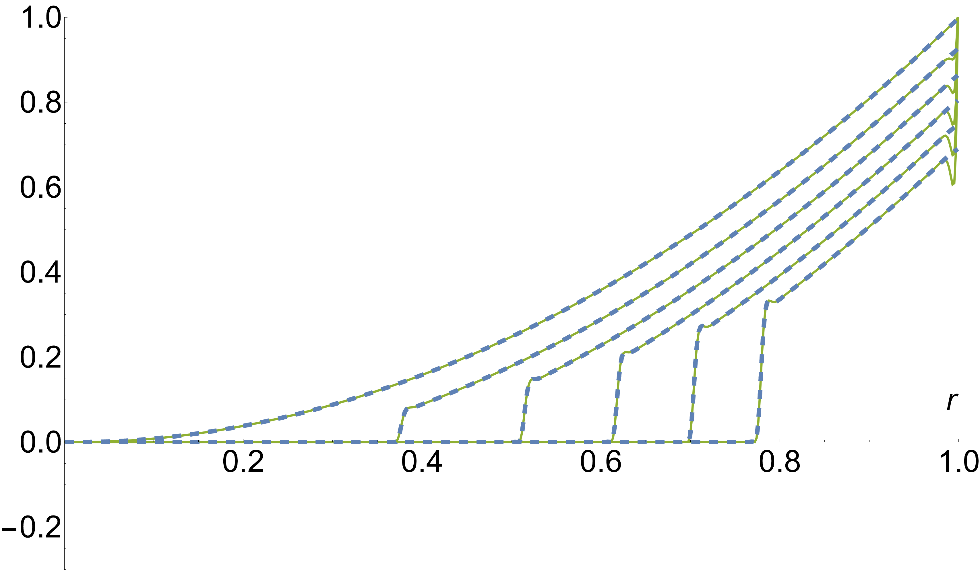


| Boundary | ||||||
|---|---|---|---|---|---|---|
|
|
| |||||
|
|
|
References
- Landau and Lifshitz (1987) L. Landau and E. Lifshitz, Fluid Mechanics Ed. (Butterworth-Heinenann, 1987).
- Trouton (1906) F. T. Trouton, On the coefficient of viscous traction and its relation to that of viscosity, Proceedings of the Royal Society of London. Series A, Containing Papers of a Mathematical and Physical Character 77, 426 (1906).
- Middleman (1995) S. Middleman, Modelling axismmetric flows: Dynamics of films, jets, and drops (Academic Press, Inc., 1995).
- Howell (1996) P. D. Howell, Models for thin viscous sheets, European Journal of Applied Mathematics 7, 321–343 (1996).
- Debrégeas et al. (1998) G. Debrégeas, de Gennes P.-G., and F. Brochard-Wyart, The life and death of ”bare” viscous bubbles, Science 279, 1704 (1998).
- Da Silveira et al. (2000) R. Da Silveira, S. Chaieb, and L. Mahadevan, Rippling instability of a collapsing bubble, Science 287, 1468 (2000).
- Slim et al. (2012) A. C. Slim, J. Teichman, and L. Mahadevan, Buckling of a thin-layer couette flow, Journal of fluid mechanics 694, 5 (2012).
- Efrati et al. (2009) E. Efrati, E. Sharon, and R. Kupferman, Elastic theory of unconstrained non-euclidean plates, Journal of the Mechanics and Physics of Solids 57, 762 (2009).
- Kumar et al. (2020) D. Kumar, T. P. Russell, B. Davidovitch, and N. Menon, Stresses in thin sheets at fluid interfaces, Nature materials 19, 690 (2020).
- Oratis Alexandros et al. (2020) T. Oratis Alexandros, M. Bush John W., A. Stone Howard, and C. Bird James, A new wrinkle on liquid sheets: Turning the mechanism of viscous bubble collapse upside down, Science 369, 685 (2020).
- Huang et al. (2007) J. Huang, M. Juszkiewicz, W. H. De Jeu, E. Cerda, T. Emrick, N. Menon, and T. P. Russell, Capillary wrinkling of floating thin polymer films, Science 317, 650 (2007).
- King et al. (2012) H. King, R. D. Schroll, B. Davidovitch, and N. Menon, Elastic sheet on a liquid drop reveals wrinkling and crumpling as distinct symmetry-breaking instabilities, Proceedings of the National Academy of Sciences 109, 9716 (2012).
- Paulsen et al. (2016) J. D. Paulsen, E. Hohlfeld, H. King, J. Huang, Z. Qiu, T. P. Russell, N. Menon, D. Vella, and B. Davidovitch, Curvature-induced stiffness and the spatial variation of wavelength in wrinkled sheets, Proceedings of the National Academy of Sciences 113, 1144 (2016).
- Box et al. (2019) F. Box, D. O’Kiely, O. Kodio, M. Inizan, A. A. Castrejón-Pita, and D. Vella, Dynamics of wrinkling in ultrathin elastic sheets, Proceedings of the National Academy of Sciences 116, 20875 (2019).
- Thomson (1904) J. J. Thomson, Xxiv. on the structure of the atom: an investigation of the stability and periods of oscillation of a number of corpuscles arranged at equal intervals around the circumference of a circle; with application of the results to the theory of atomic structure, The London, Edinburgh, and Dublin Philosophical Magazine and Journal of Science 7, 237 (1904).
- Bowick et al. (2000) M. J. Bowick, D. R. Nelson, and A. Travesset, Interacting topological defects on frozen topographies, Physical Review B 62, 8738 (2000).
- Bausch et al. (2003) A. Bausch, M. J. Bowick, A. Cacciuto, A. Dinsmore, M. Hsu, D. Nelson, M. Nikolaides, A. Travesset, and D. Weitz, Grain boundary scars and spherical crystallography, Science 299, 1716 (2003).
- Nelson (2002) D. Nelson, Defects and geometry in condensed matter physics (Cambridge University Press, 2002).
- Bandurin D. et al. (2016) A. Bandurin D., I. Torre, K. R. Krishna, M. Ben Shalom, A. Tomadin, A. Principi, H. Auton G., E. Khestanova, S. Novoselov K., V. Grigorieva I., A. Ponomarenko L., K. Geim A., and M. Polini, Negative local resistance caused by viscous electron backflow in graphene, Science 351, 1055 (2016).
- Jesse et al. (2016) C. Jesse, K. Shi Jing, W. Ke, L. Xiaomeng, H. Achim, L. Andrew, S. Subir, K. Philip, T. Takashi, W. Kenji, A. Ohki Thomas, and F. K. Chung, Observation of the dirac fluid and the breakdown of the wiedemann-franz law in graphene, Science 351, 1058 (2016).
- Moll Philip J. et al. (2016) W. Moll Philip J., K. Pallavi, N. Nabhanila, S. Burkhard, and P. Mackenzie Andrew, Evidence for hydrodynamic electron flow in PdCoO2, Science 351, 1061 (2016).
- (22) The original form of Eqs. (7) in Ref. Howell 1996 ignores the contribution in (7b), whereas the version in Ref. Mahadevan et al. 2010 is valid only for small perturbations of a hemispherical shape.
- Stone (1990) H. A. Stone, A simple derivation of the time dependent convective diffusion equation for surfactant transport along a deforming interface, Physics of Fluids A: Fluid Dynamics 2, 111 (1990).
- Buckmaster et al. (1975) J. Buckmaster, A. Nachman, and L. Ting, The buckling and stretching of a viscida, Journal of Fluid Mechanics 69, 1 (1975).
- Ribe (2001a) N. Ribe, Bending and stretching of thin viscous sheets, Journal of Fluid Mechanics 433, 135 (2001a).
- Le Merrer et al. (2012) M. Le Merrer, D. Quéré, and C. Clanet, Buckling of viscous filaments of a fluid under compression stresses, Physical review letters 109, 064502 (2012).
- Pfingstag et al. (2011) G. Pfingstag, B. Audoly, and A. Boudaoud, Linear and nonlinear stability of floating viscous sheets, Journal of fluid mechanics 683, 112 (2011).
- Srinivasan et al. (2017) S. Srinivasan, Z. Wei, and L. Mahadevan, Wrinkling instability of an inhomogeneously stretched viscous sheet, Physical Review Fluids 2, 074103 (2017).
- O’Kiely et al. (2019) D. O’Kiely, C. Breward, I. Griffiths, P. Howell, and U. Lange, Out-of-plane buckling in two-dimensional glass drawing, Journal of Fluid Mechanics 869, 587 (2019).
- Ribe (2001b) N. Ribe, Bending and stretching of thin viscous sheets, Journal of Fluid Mechanics 433, 135 (2001b).
- Howell (2022) P. Howell, private communication (2022).
- Landau and Lifshitz (1986) L. Landau and E. Lifshitz, Theory of Elasticity Ed. (Butterworth-Heinenann, 1986).
- Irvine et al. (2010) W. T. Irvine, V. Vitelli, and P. M. Chaikin, Pleats in crystals on curved surfaces, Nature 468, 947 (2010).
- Gurzhi (1963) R. N. Gurzhi, Minimum of resistance in impurity-free conductors, Journal of experimental and theoretical physics 17, 521 (1963).
- Andreev et al. (2011) A. V. Andreev, S. A. Kivelson, and B. Spivak, Hydrodynamic description of transport in strongly correlated electron systems, Phys. Rev. Lett. 106, 256804 (2011).
- Hartnoll (2015) S. A. Hartnoll, Theory of universal incoherent metallic transport, Nature Physics 11, 54 (2015).
- Levitov and Falkovich (2016) L. Levitov and G. Falkovich, Electron viscosity, current vortices and negative nonlocal resistance in graphene, Nature Physics 12, 672 (2016).
- Scriven (1960) L. E. Scriven, Dynamics of a fluid interface equation of motion for newtonian surface fluids, Chemical Engineering Science 12, 98 (1960).
- Mahadevan et al. (2010) L. Mahadevan, R. Bendick, and H. Liang, Why subduction zones are curved, Tectonics 29 (2010).
- Van De Fliert et al. (1995) B. W. Van De Fliert, P. D. Howell, and J. R. Ockenden, Pressure-driven flow of a thin viscous sheet, Journal of Fluid Mechanics 292, 359–376 (1995).
- Anderson et al. (2006) M. Anderson, A. Bassom, and N. Fowkes, Exact solutions of the laplace-young equation, Proceedings of the Royal Society A: Mathematical, Physical and Engineering Sciences 462, 3645–3656 (2006).
- Howell (1999) P. D. Howell, The draining of a two-dimensional bubble, Journal of Engineering Mathematics 35, 251–271 (1999).
- Obreimoff (1930) J. Obreimoff, The splitting strength of mica, Proceedings of the Royal Society A: Mathematical, Physical and Engineering Sciences 127, 290–297 (1930).
- Brenner and Gueyffier (1999) M. Brenner and D. Gueyffier, On the bursting of viscous films, Physics of Fluids 11, 737 (1999).
- Savva and Bush (2009) N. Savva and J. Bush, Viscous sheet retraction, Journal of Fluid Mechanics 626, 211 (2009).
- Bartlett et al. (2023) C. Bartlett, A. T. Oratis, M. Santin, and J. C. Bird, Universal non-monotonic drainage in large bare viscous bubbles, Nature Communications 14, 877 (2023).
- Davidovitch et al. (2012) B. Davidovitch, R. Schroll, and E. Cerda, Nonperturbative model for wrinkling in highly bendable sheets, Physical Review E 85, 066115 (2012).
- Davidovitch et al. (2019) B. Davidovitch, Y. Sun, and G. M. Grason, Geometrically incompatible confinement of solids, Proceedings of the National Academy of Sciences 116, 1483 (2019).
- Taffetani and Vella (2017) M. Taffetani and D. Vella, Regimes of wrinkling in pressurized elastic shells, Philosophical Transactions of the Royal Society A: Mathematical, Physical and Engineering Sciences 375, 20160330 (2017).