Nested spheroidal figures of equilibrium
I. Approximate solutions for rigid rotationsNested spheroidal figures of equilibrium
I. Approximate solutions for rigid rotations–???
Abstract
We discuss the equilibrium conditions for a body made of two homogeneous components separated by oblate spheroidal surfaces and in relative motion. While exact solutions are not permitted for rigid rotation (unless a specific ambient pressure), approximations can be obtained for configurations involving a small confocal parameter. The problem then admits two families of solutions, depending on the pressure along the common interface (constant or quadratic with the cylindrical radius). We give in both cases the pressure and the rotation rates as a function of the fractional radius, ellipticities and mass-density jump. Various degrees of flattening are allowed but there are severe limitations for global rotation, as already known from classical theory (e.g. impossibility of confocal and coelliptical solutions, gradient of ellipticity outward). States of relative rotation are much less constrained, but these require a mass-density jump. This analytical approach compares successfully with the numerical solutions obtained from the Self-Consistent-Field method. Practical formula are derived in the limit of small ellipticities appropriate for slowly-rotating star/planet interiors.
Keywords:
Gravitation — stars: interiors — stars: rotation — planets and satellites: interiors — Methods: analytical1 Introduction
According to the theory of figures (Chandrasekhar 1969), a homogeneous body bounded by a spheroidal surface with semi-minor axis and semi-major axis is in self-gravitating equilibrium if the rotation rate and the mass density are linked by
| (1) |
where is the ellipticity, is the constant of gravitation, and
| (2) |
This result is due to Maclaurin. In which conditions a body made of two rotating components separated by spheroidal surfaces can be a figure of equilibrium, and what types of solutions are permitted? These questions have been examined in details more than one century ago by Hamy, Poincaré and others in the specific context of the Earth and planets, already in the multilayer case (Love et al. 1914); see also Pohánka 2011 and Ragazzo 2018. As most systems in the Universe are significatly flattened by rotation and exhibit a certain internal stratification, the problem is obviously of wider interest. The interior of stars is concerned, with, for instance, the discovery of limits in the mass and size of nuclear cores (Schönberg & Chandrasekhar 1942; Maeder 1971; Rucinski 1988; Rozelot et al. 2001; Kiuchi et al. 2010; Kadam et al. 2016). Galactic halos hostings disks represent another class of composite systems, although mainly non-collisional, the equilibrium and stability of which have been studied from theory of ellipsoidal figures (Abramyan & Kaplan 1974; Abramyan & Kaplan 1975; Durisen 1978; Robe & Leruth 1984; Smeyers 1986; Caimmi & Secco 1990; Martinez et al. 1990).
The establishment of the conditions for the existence of nested, spheroidal figures is a tricky problem, even under the assumptions of incompressibility and rigid rotation. Actually, with only two components, this is already a four dimensional problem. Poincaré 1888 proved that only configurations involving confocal spheroidal surfaces are viable if all layers rotate synchroneously, while Hamy 1890 pointed out that such states require a density inversion (the mass density increases from centre to surface); see also Montalvo et al. 1983. In this article, we present a concise survey of the -layer problem and focus on oblate spheroidal, bounding surfaces (in the meridional plane, the layers are separated by perfect ellipses). The more complicated case of a multilayer system is treated in a forthcoming article (paper II). The two components are homogeneous and treated as collisional fluids in the sense that the two phases do not mix. In contrast with most previous investigations, we initially relax the assumptions of confocality, coellipticity and common rotation rate. The question of the rotation laws is central. According to Poincaré’s and Hamy’s theorems (Poincaré 1888; Moulton 1916), global rotation is not permitted neither for coelliptical nor for confocal configurations. Nevertheless, the numerical approach (Basillais & Huré 2021) shows that, for global rotation, i) the “cores” are generally more spherical than the surrounding layers, and ii) the bounding surfaces are remarkably close to ellipses. This is observed not only in the incompressible case but for a wide range of polytropic indices. This article is therefore partly motivated by this apparent paradox. In a remarkable monograph, Hamy 1889 has shown that rigid rotation is verified in a first approximation for small ellipticties. Here, we give an extended version of this analysis based on an expansion in the confocal parameter (rather than in the ellipticities). Besides, we wish to go beyond the “simple” case of global rotation and seek for solutions involving asynchroneously rotating layers.
There are different options to treat the problem: i) directly from the three components of forces (Hamy 1889, e.g.), ii) from the modified Lane-Emden equation (Caimmi 1986), iii) from the conservation of energy (Montalvo et al. 1983), and iv) from the Virial equations, which is probably the most powerful approach (Chandrasekhar 1969; Maeder 1971; Abramyan & Kaplan 1974; Durisen 1978; Brosche et al. 1983; Caimmi & Secco 1990, e.g.). In this paper, we follow the second path, and directly make use of the Bernoulli equation. We show that, to the first order in the confocal parameter (see below), the problem admits solutions compatible with the rigid rotation law. This is discussed in Sects. 2 and 3. We then examine the case of global rotation (type-C solutions; same rotation rate for both components) in Sect. 4. We consider the more general situation where the embedded spheroid and the surrounding layer are in relative motion (type-V solutions) in Sect. 5. A few practical formula valid in the limit of small ellipticities are derived in Sect. 6. Exact solutions corresponding to differentially rotating components are given in the concluding section. A basic (non-optimized) F90-code is appended.
2 The equations of equilibrium
2.1 Hypothesis and notations
Inside a Maclaurin spheroid (see the Introduction), the pressure of matter varies according to the Bernoulli equation
| (3) |
where the constant can be evaluated at the center of coordinates, and is the interior gravitational potential. In polar cylindrical coodinates , this function writes
| (4) |
where
| (5) |
and is the dimensionless polar radius. Note that ; see (2). The knowledge of the external potential is essential to treat the problem of nested figures. It is given by (Chandrasekhar 1969; Binney & Tremaine 1987, e.g.)
| (6) |
where the ’s are still given by (5),
| (7a) | |||||
| (7b) | |||||
| (7c) |
In (7a), is clearly the root of a second-degree polynomial. In the present case, only the largest positive root is relevant. For a given pair , this quantity varies with and ; see Sect. 3. It can be verified that (4) and (6) coincide at the boundary , where .
We consider that this spheroid (we use the subscript for associated quantities), is embedded inside a homogeneous body (subscript ), called the “host”, which shares the same axis of revolution and same plane of symmetry (and subsequently, the same center). This is a hollow body, internally bounded by (i.e. the common interface) and externally bounded by a larger, spheroidal surface , with semi-minor axis and semi-major axis . The spheroidal surfaces are not allowed to intersect. This two-component system is depicted in Fig. 1a. Another important assumption is that there is no exchange or travel of matter between the two components. In a collisionaless system, as in galaxies, this permitted (Abramyan & Kaplan 1975; Caimmi 1986, e.g.).

According to the common convention (Kelvin et al. 1883; Perek 1950), the host is called a “focaloid” when and are confocal, which corresponds to . It is called a “homoeoid” when and are similar or homothetic surfaces, which means . We can introduce the word “heteroeoid” to refer to the general case where and are neither confocal nor similar (but still not intersecting). Although a selection of preferred configurations will be perfomed, we do not impose any constraint yet on the ellipticities and , and each one can run over the full range . If denotes the fractional size of the embedded spheroid, the condition of complete immersion writes
| (8) |
An important ingredient of the problem is the mass-density jump11 1 The density contrast of the nested spheroid with respect to the host is . defined as
| (9) |
It must be a positive constant, with a preference for
| (10) |
otherwise the host is more dense than the embedded body (density inversion). With these notations, the total volume of the system is and the total mass is given by
| (11) |
which leads to the mean mass-density and to the fractional masses, namely
| (12) |
for the embedded spheroid and for the host.
2.2 The equations of equilibrium
Working with exact spheroidal surfaces offers a great mathematical simplification as it fixes the gravitational potential. The global equilibrium requires that (3) holds for each component. For the embedded spheroid, the relevant gravitational potential is found from superposition by considering (4) with appropriate settings for the mass densities and for the ’s and ’s involved, namely
| (13) |
where
| (14) |
In these conditions, the equilibrium of the embedded spheroid, assumed in rigid rotation, is dictated by (3) and (13), namely
| (15) |
where is the central pressure. Inside the host, the gravitational potential combines an interior form and an exterior form. From (4) and (6), we have
| (16) |
where
| (17) |
and and are still given by (7b) and (7c) respectively, but for . The ’s depend clearly on three parameters, namely , and , but, in contrast, with the ’s, these quantities also depend on , like and , and subsequently on and . Again, assuming rigid rotation (at a rate ), the Bernoulli equation for the host writes
| (18) |
where the constant can be derived at the surface. For instance at point A (see Fig. 1), provided the ambient medium brings no contribution to the pressure, we have
| (19) |
where the values of , and required at point A2 are easily found (see below).
Another decisive equation is the requirement of pressure balance at the connection between the two components, namely
| (20) |
The continuity of the pressure and the continuity of the gravitational potential at means that the mass densities and on both sides of the interface must be coherent with the Bernoulli equations (15) and (18), which implies a jump, i.e. . Eventually, a discontinuity in the rotation rates can occur in addition. From this point of view, the fact that and can differ at a given radius does not seem in contradiction with the Poincaré-Wavre theorem. Barotropic systems indeed require that the rotation rate must be constant on cylinders (Tassoul 1978; Amendt et al. 1989). Here, howewer, we have two components in contact and the change in the rotation law at the interface is associated with a coherent change in the mass density (Montalvo et al. 1983; Caimmi 1986; Kiuchi et al. 2010, e.g.).
2.3 Note on the pressure on the polar axis
A nested equilibrium is in principle found by solving (15), (18) and (20), with the conditions (8) and (10). As the centrifugal forces vanish on the rotation axis (this should be true for rotation laws other than rigid), the pressure at point A1 of the polar axis and the central pressure can already be calculated. From (15), (18) and (20), we actually find
| (21) |
and
| (22) |
These two expressions are exact (Robe & Leruth 1984).
3 The -parameter out of confocality
3.1 Conditions for approximate rigid rotations
As outlined above, the -parameter is a key-quantity of the problem. While is characterized by , we see from (7a) that generally involves a continuum of values for ranging from (on the polar axis; see point A2 in Fig. 1a) to (at the equator, i.e. point B2). If we define
| (23) |
we have at the two end-points
| (24) |
where
| (25) |
is the “confocal” parameter. We then have
| (26) |
Except if is confocal with (in which case ), we see from (7a) and (23) that varies along the surface according to
| (27) |
where
| (28) |
The relevant value for is the largest, positive root of this equation. It is given by
| (29) |
which is clearly not constant with the cylindrical radius. It means that, at the surface of the system, the ’s depend on and , with the consequence that (18) cannot be satisfied for rigid rotation. But there are two exceptions: i) and are confocal, or ii) the ambient medium exerts a specific, non-constant pressure along . The first property is known for long (Poincaré 1888), but it implies (Hamy 1890; Montalvo et al. 1983); see below. Regarding the second one, must partially or totally neutralize the terms in coming from . Due to the continuity of the gravitational potential, the pressure inside the host can remain quadratic with the radius along any intermediate spheroidal surface located from down to . Then, according to (15) and (20), the embedded spheroid can be in rigid rotation too, and the pressure inside can be either quadratic with the cylindrical radius or a constant. It follows that a sufficient condition for the two homogeneous components of a heterogeneous systems separated by spheroidal surfaces be in rigid rotation is the existence of an ambient pressure. Note that the origin of this ambient pressure is preferably a photon field, otherwise there would be an extra contribution to gravity that would affect .
3.2 Orders zero and one in the confocal parameter
It follows from the above discussion that, in the absence of any ambient pressure, any solution obtained with rigid rotations must be regarded as an approximation, as considered in Hamy 1889. Since the Bernoulli equation is already quadratic in and (and easily convertible in a function of on any ellipse), it is interesting to expand as a series of . In this purpose, the square root in (29) is rewritten as
| (30) |
and subsequently expanded. Because , we have . It follows that the term supporting in the above expression is, in absolute, less than unity provided . This excludes infinitely flat configurations (i.e. disks). In these conditions, the solution can be put into the form
| (31) |
where the factorization by is required as for for any . So, we have at order zero in . As first-order, we retain the next terms compatible with (24), namely
| (32) |
which implies i) (i.e. is close to a sphere) or ii) (the embedded spheroid has small size) or iii) (the embedded spheroid is close to a sphere). Thus, these latter conditions do not necessarily imply that the two spheroidal surfaces and are simultaneously close to spheres. This is in contrast with respect to the classical appraoch (Hamy 1889; Chandrasekhar & Roberts 1963, e.g.).
We see that (32) is simple and attractive as it yields the correct values at the two end-points A2 and B2 of ; see (24). Besides, (31) means that any regular function of or of is an infinite series of . The ’s which are needed in (18) enter into this category. While we will make no use of such an information, it is interesting to see how these quantities depend on along and on the confocal parameter . If we Taylor-expand around the value at one of the end-points, for instance at point B2 on the equator, we get
| (33) |
Unfortunately, this formula, which has to be truncated in practice, does not lead to the required value on the polar axis (i.e. at point A2 in Fig. 1), but we already see that . With a finite difference, we have
| (34) |
| (35) |
from (23) and (31). We therefore see that, at the lowest order in , all the ’s in (18) remain unsensitive to the radius, and we have . To the first order in , all the ’s in (18) bring a quadratic contribution in , which, depending on , and , reinforces or decreases the quadratic contribution explicitely present in (16). Accordingly, contains not only terms in but also terms in as well (see Sect. 7). The limit of rigid rotation is therefore reached. Whatever the variation of the ’s along , the values at the two-end points A2 and B2 are perfectly accessible from (23) and (26), and we will use these values to go beyond order zero. Note that, if is indeed close to , the derivatives , and subsequently the term inside the parenthesis in the right-hand-side of (34), are expected to be small-amplitude corrections.
4 Type-C solutions : the interface is a surface of constant pressure
4.1 Rotation rate and mass-density jump. Example
We have now to determine the rotation rate for the two components and the conditions that these are real and positive values. We first focus on order zero (i.e. ). The first family of solution is obtained by assuming that the interface is a surface of constant pressure (Lyttleton 1953, e.g.). On this surface, we have
| (36) |
As the do not depend on , the rotation rate of the embedded spheroid is directly deduced from (15), namely
| (37) |
which clearly differs from (1). This result is already known (Abramyan & Kaplan 1974, e.g.). If, for convenience, we express the ’s in units of by setting
| (38) |
The rotation rate of the host is obtained from (18) at where the pressure is zero. On this surface, we have
| (41) |
which can be injected in (18). At the lowest order, the ’s do not depend on . The term in in this expression must therefore vanish, which yields the rotation rate, namely
| (42) |
Let us now express the pressure in the host at the interface . Still using (18) but onto , which is assumed to be a surface of constant pressure, we see that the term in has to be null, again. The rotation rate is then given by
| (43) |
which must be identical to (42). It is clear from (14) and (17) that for . As a consequence, . Rotation is therefore global. Since all terms in are neutralized by the centrifugal potentials, and due to (20), the pressure is a constant all along the interface , which validates the initial assumption. The interface is therefore a surface of constant effective (gravitational and centrifugal) potential. This is called a “type-C solution” in the following. So, in the conditions of the approximation where , in a heterogeneous systems made of two homogeneous components separated by spheroidal surfaces and rotating at the same rate, the pressure at the common interface is a constant. We see by equating (40) to (42) that the necessary condition for global rotation is that the function
| (44) |
admits at least one zero over the range of interest. Solving the equation requires in principle a full survey of the parameter space, which is -dimensional, but it happens that in (44) is easily accessible from the other parameters as it is observed in the confocal case (Montalvo et al. 1983, e.g.), namely
| (45) |
At order one in , the rotation of the embedded spheroid is unchanged, as quoted, but varies slightly from point A1 to point B1 along the interface, which modifies . For the host, we use (18) at these two end points, and we find
| (46) |
which can be put in a dimensionless form from (16) and (38). In these conditions, it can then be shown that (42), (44) and (45) keep the same form provided the quantity is replaced by
| (47) |
where
| (48) |
which is therefore to be evaluated at points A2 and B2. This correction represents the deviation to confocality and it vanishes when .

| configuration A | ||||
|---|---|---|---|---|
| this work | DROP† | this work | DROP† | |
| order | order | |||
| input data | ||||
| ∗value on the polar axis | ||||
| †SCF-method (Basillais & Huré 2021) | ||||
Figure 2 displays an example of equilibrium in the form of contours levels for the pressure and for the gravitational potential22
2
In the graphs and tables, the pressure is given in units of and the potential is in units of . obtained for a canonical triplet . The main input and output quantities are listed in Tab. 1 for order (column 2) and for order (colmun 4). In this example, the confocal parameter is about , and the mass-density jumps are and , respectively. By comparing the exact root of the second-order polynomial (27) with as given by (32), we can easily verify that the approximation is justified. This is corroborated by the results obtained with the DROP-code (see Tab. 1, columns 3 and 5) that solves numerically the -layer problem from the Self-Consistent-Field (SCF) method33
3
This code includes an accurate determination of the bounding surfaces at each step of the SCF-cycle. In this process, the location of point B2 is not known in advance (output). (Basillais &
Huré 2021). We show in Fig. 3 the absolute deviation between the “true” bounding surfaces and the ellipses and , which is of the order of a few purcents. Equilibrium values (rotation rate, pressures, mass) are reproduced with a relative error of typically at order 0, while this is of the order of at order 1.


4.2 Singular cases. Condition of positivity
There is a pending difficulty in the above relationship since can diverge. This corresponds to a highly condensed embedded spheroid relative to the host, which situation can be associated with Roche systems (Jeans 1928); see below. The singularity occurs for finite values of the parameters when the denominator in (45) tends to (the sign of changes), i.e. for
| (49) |
Figure 4 displays in the form of contour levels. This quantity takes large positive values in the top-left part of the -plane where roughly, and it takes small, negative values elsewhere. The ratio of the st-order correction to the leading term is shown in Fig. 5 in the -plane (this ratio depends on only these two parameters). It turns out that the correction is of small amplitude in relative in a wide part of the plane around the line , except in three domains typically, namely: i) the vicinity of the line where vanishes (see Tab. 2 for a sample of solutions of ), ii) when is close to unity (right part of the plot; the host resembles a flat disk), and iii) when is close to unity (top part of the plot; the embedded ellipsoid is very flat, with a radius close to the radius of the host).
We see from (45) that the magnitude and the sign of the mass-density jump remain hard to guess without considering numbers in the formula. The reason is that and take opposite signs in the same domain of the -plane. Besides, is not a monotonic function of the ellipticity , with a maximum value at . In fact, for , we have and the numerator in (45) is therefore poisitve and dominated by . In the same time, , making the denominateur of small amplitude, and eventually negative (unless is small). The mass-density jump is large in absolute. In order to make the denominator positive (and subsequently to get a positive mass-density jump), must be small enough. This is the case of spheroids with a low oblateness and a massive host. The denominator in (45) reaches zero by increasing , and it becomes negative, which leads to . Note that configurations with corresponding to flat ellispoidal surfaces can be generated. This happens in the decreasing part of the function when ), but this involves -values close to unity.
Physically relevant solutions must be such that . Since the two rates are equal and , this inequality writes, from (40) and (42)
| (50a) | |||||
| (50b) |
It follows from the first condition that is inconditionally positive in the domain where . From Fig. 4, we see that this domain corresponds to . Such a condition, however, leads to small positive values, or even negative values, of . In contrast, from (50b), is inconditionally positive in the domain where , i.e. for from Fig. 4. This is precisely a situation that favours large, positive values of the mass-density jump, which also makes (50a) easily fulfilled. We conclude that the most favorable conditions for the existence of nested figures of equilibrium in global rotation (type-C solutions) are met for and small -values.
4.3 Special cases
Confocality. This geometry is met for . In this case, the st-order correction is zero, and (45) reads
| (51) |
A quick scan at the full domain shows that . Confocal states are exact solutions (Poincaré 1888), but the host must be more dense than the embedded spheroid, which is a highly unstable situation. This agrees with known results (Hamy 1890; Montalvo et al. 1983), and this is still true in the conditions of the actual approximation where : a heterogeneous body made of two homogeneous components separated by confocal spheroids cannot be in global rotation (unless a density inversion).

Coellipticity. For , we have , and so, from (44)
| (52) |
where
| (53) | ||||
If we exclude and as trivial solutions, keeps the same sign and does not vanish inside the relevant range , as Fig. 6 proves. This is true at orders and in the -parameter, and it does not depend on . Again, this agrees with Hamy 1889, and this is even true in the conditions of the approximation where : a heterogeneous body made of two homogeneous components separated by similar spheroids cannot be in global rotation.
The Maclaurin solution. For , the density of the host and the density of the embedded spheroid become equal. We have respectively from (40) and (42)
| (54a) | |||||
| (54b) |
As , the two rotation rates merge only if . This result does not depend on . The two components are indistinguishable and rotate in a synchroneous manner: this is basically a single object (Maclaurin) spheroid.


Generalized Roche systems. Another interesting situation is met for . In this case, the host is a rarefied medium compared to the embedded spheroid. From (40), we have , which is identical to (1). The embedded spheroid rotates by itself and carries away the host which has a negligible contribution to gravity. Actually, from (42), we get , and by using (49), we recover . We can expand the expression for in the limit . We have , and so we find
| (55) |
where we have included the first-order correction. If we now express the rotation rate at the surface of the host (point B2 of the equator; see Fig. 1), as it is imposed by the embedded spheroid (now reduced to a point mass), we get , which is equal to (55) for . This value is in agreement with Roche’s model, although the true surface is not an ellipse (Maeder 2009, e.g.). This calculus can in principle be repeated for any value of , in which case the equation , if exists, yields a relationship between and . As done in Jeans 1928, we have considered the ellipticity of the embedded (Maclaurin) spheroid at the bifurcation point towards the Jacobi sequence, namely where (Chandrasekhar 1969). The numerical solution is plotted in Fig. 7. It fulfills (8) for . For the lowest value, the host has zero thickness at the pole and the largest equatorial extension, while for , it has zero thickness all along (which is therefore confunded with ). The volume of the host goes through a maximum at , which is close to the exact estimate by Jeans 1928, .
5 Type-V solutions : the pressure varies along the interface
We get the second family of solution in a very similar way, by considering the host first. Clearly, (42) is still valid, with or without the st-order correction; see (47). The interface pressure, as imposed by the host, is therefore deduced from (18), and it must be the same as the pressure delivered by the embedded spheroid. The main difference with above comes from (43), which is no more imposed. This just means that the interface pressure participates in the mechanical support like the gravitatinal term in the Bernoulli equation, and it varies quadratically with the radius along . This is called a “type-V solution” in the following. By combining (15), (18) and (20), we find
| (56) |
which yields . We see that, if the quantity inside the curly brackets is zero, whatever the mass density jump, then : this is precisely the type-C solution; see (37). Type-C solutions form a therefore a subset of type-V solutions. The other important point is that the two components can be in relative rotation only if .
Figure 8 displays an example of a type-V solution obtained for the same triplet as for Fig. 2, but with (i.e. twice the value required by the type-C solution). The st-order correction has been accounted for. The key quantities are given in Tab. 3 (column 2). In this case, the rotation rate of the embedded spheroid is slightly larger than for the host. We can get a reverse situation if the mass-density jump is below the value corresponding to the type-C solution. We give in Tab. 3 (column 4) the results obtained for . Figure 9 shows the interface pressure as a function of the radius for these two examples. We notice that the variation from the pole to the equator is very weak, because the ellipticities of the two components are close to each other. Again, the comparison with the equilibrium states computed from the SCF-method (see Tab. 3, columns 3 and 5) is very satisfactory as the relative deviations are of the order of .

| configuration B | configuration C | |||
| this work | DROP† | this work | DROP† | |
| input data | ||||
| ∗value on the polar axis | ||||
| †SCF-method (Basillais & Huré 2021) | ||||
It is interesting to see how the approximation behaves when the ellipticities are not “small”. We show in Figs. 10, 11 and 12 three typical type-V solutions obtained for the input parameters listed in Tab. 4. Again, the st-order correction has been included in the calculations. We have conserved the same mass-density jump as above. The first case is a highly flattened embedded spheroid and a weakly oblate host. The -parameter is still lower than unity, but now positive. It means that the host is less oblate than the confocal configuration would produce. The approximation is still very good (the line where the pressure naturally vanishes almost coincides with ). The rotation rate of the host is lower that for the embedded spheroid. The second case corresponds to two hilghly flattened bodies, again with a low -parameter. The third example is a highly flattened host containing a moderately oblate, embedded body. The -parameter is close to unity in absolute. The approximation of rigid rotation therefore fails. The variation of is no more dominated by . This is visible in the figure since the line where and are no more confunded. Note that is beyond the threshold for dynamical stability (for a single body), and it would be interested to see the role of the host; see Sect. 7.


| config. D | config. E | config. F | |
| input data | |||
| ∗value on the polar axis | |||
| †SCF-method (Basillais & Huré 2021) | |||
5.1 Conditions of positivity
Because is free, type-V solutions are less contrained than type-C solutions. There are, however, still restrictions on the parameter sets leading to physically relevant solutions. The two rotation rates must be positive (double condition). Again, it is difficult to conclude since (42) and (56) are complicated funtions of , , and . If we omit the st-order correction, the condition writes
| (57) |
and it is automatically verified as soon as and (10) holds. We see from Fig. 4 that this occurs for moderate/large values of and small/moderate values of . In the other part of the domain where , both and play a critical role. The criterion can still be satisfied either with a value of very close to unity or for a small -parameter.
The second condition that must be examined simultaneously with (57) corresponds to . If we rewrite (56) as
| (58) |
we see that the term inside the brackets can eventually be negative, but it must not exceed , in absolute. Again, for , we have , which always ensures an equilibrium; see Fig. 4. For large, positive values of , which occurs when the embedded boby is very flat with respect to the host, can become negative. This situation can be “neutralized” in three ways: i) the mass-density jump is large enough in the sense , ii) in constrast, which decreases the term inside the brackets (we are close to global rotation in this case), and iii) , which occurs for extreme values of .
5.2 Note about confocal and coelliptical configurations
For , (42) reads
| (59) |
which is clearly a positive quantity for , and is easily deduced from (58). Since , is negative, meaning that , but . In agreement with Montalvo et al. 1983, and in the conditions of the approximation where , the two homogeneous components of a heterogeneous body separated by confocal spheroids are necessarily in relative rotation. Note that (59) also writes
| (60) |
where is the mean density of the system.
By setting in (56), we find
| (61) |
| (62) | ||||
We see that the two rotation rates are identical only when (single spheroid case), which is in agreement with the discussion in Sect. 4: the two homogeneous components of a heterogeneous body separated by similar spheroids are necessarily in relative rotation, in the conditions of the approximation where .
6 Practical formula for the slow-rotation limit
Cases with are of great interest for stars/planet interiors, as they correspond to the slow-rotation limit (the deformation with respect to sphericity is smaller than unity). It is generally admitted that interior layers are also characterized by small ellipticities, but there is no evidence that this occurs systematically, and this may depend on the process of formation, accretion and occasionally of differentiation of the entire body. If we set (which is not necessarily small) and expand (42), (48) and (58) for small ellipticities, we find (see the Appendix A for more details)
| (63) | ||||
for the host, and
| (64) | ||||
for the embedded spheroid. These formula include the st-order correction. For type-C solutions, (64) directly yields
| (65) | ||||
By equating this expression to (63), we get the value of the mass-density jump; see (81) in the Appendix A. If is significantly larger than unity or if a lower precision is sufficient, we can simplify more these formula and forget the st-order correction. In these conditions, we get
| (66a) | |||||
| (66b) |
For type-C solutions, (66b) yields
| (67) |
which is equal to (66a). Again, this gives the link between the mass-density jump, the size and the ellipticity of the embedded spheroid relative to the host, namely
| (68) |
Figure 13 compares these approximations with the references (42) and (58) for the pair already considered in the preceeding sections, and three values of the -parameter. We see the excellent agreement between various formula. While the st-order correction is, as expected, very precise, the leading term, alone, is already remarkably close to the reference, in particular for the embedded spheroid.

It is interesting to notice that (68) is compatible with the conclusions drawn in Sect. 4: global rotation is not possible for coelliptical configurations ( for ) and for confocal states ( for ) as well. Another important point concerns the magnitude of . By reversing (68), we find
| (69) |
and we see that is larger than unity in the whole domain of interest provided . This is in agreement with Hamy 1889, and in coherence with what is experimentally observed from the SCF-method (Basillais & Huré 2021). It follows that, in the conditions of the actual approximation where , in a heterogeneous body made of two homogeneous, synchroneously rotating components separated by spheroidal surfaces, the embedded spheroid is necessarily more spherical (less oblate) than the host. Note that when (the embedded spheroid has small size), while for (the host has small size).
For type-V solutions, the ratio of the rotation rates is directly found from (66a) and (66b), namely
| (70) |
Typically, this ratio is smaller than unity for large values of the -parameter (the embedded spheroid is very close to spherical) and close to unity (the relative size/volume of the host is small).
| input parameters | equation | comment | |
| ellipticity of | |||
| ellipticity of | |||
| fractional radius of the embedded spheroid | |||
| mass-density jump | useless for type-C solutions | ||
| intermediate data | |||
| confocal parameter | (25) | required | |
| various coefficients | , and | (5) | |
| (24) | exact values at points A2 and B2 | ||
| and | (26) | ||
| leading term | (39) | ||
| rst-order correction | (47) | ||
| pressure | |||
| surface | |||
| interface (pole value) | (22) | see (20) | |
| central value | (21) | ||
| rotation rate (type-V solution) | |||
| host | (42) | ||
| small ellipticities (order 0) | (66a) | and | |
| small ellipticities (order 1) | (63) | ||
| embedded spheroid | (58) | ||
| small ellipticities (order 0) | (66b) | and | |
| small ellipticities (order 1) | (64) | ||
| rotation rate (type-C solution) | |||
| both components | (40) or (42) | ||
| mass-density jump | (45) | ||
| small ellipticities (order 0) | (67) and (68) for | ||
| small ellipticities (order 1) | (63) or (64) and (81) for | ||
7 Conclusion and perspectives
This article is a novel contribution to the theory of figures (Chandrasekhar 1969). We have established the equilibrium conditions for a heterogeneous body made of two homogeneous components bounded by concentric and coaxial, spheroidal surfaces and in relative rotation. This special geometry offers a great mathematical simplification since the gravitational potential of spheroids is known in closed form. Regardless of the rotation laws, we can consider a wide range of flattenings that is difficult to reach through perturbative methods (Chandrasekhar 1933; Caimmi 2016). Various collisional systems are concerned, like stars and planets and gaseous envelopes hosting protostars. Due to the hypothesis of incompressibility, however, the best targets for this study are rocky/icy planets surrounded by a solid/liquid envelope. A generalization of the present approach to the multi-layer case is proposed in Huré 2021.
The two-component problem depends on four parameters, three geometrical parameters (the ellipticities and the fractional size of the immersed body) and one thermodynamical parameter (the mass-density jump). This already renders the analytical treatement complicated. Except for a specific ambient pressure and for confocal configurations (Poincaré’s theorem), there is no exact solution to the problem of nested spheroids compatible with rigid rotation. In the latter case, however, a mass-density inversion is necessary, which is highly improbable for stability reasons (Hamy 1890; Moulton 1916; Montalvo et al. 1983).
As argued in Hamy 1889, states of rigid rotations are valuable in a first approximation only for small ellipticies. As shown here, the confocal parameter defined by (25) enables to consider much more configurations than those accessible by assuming small ellipticities. This work can therefore be regarded as a prolongation of Hamy’s approach. When , the problem admits typically two families of solutions, depending on the interface pressure. For type-C solutions, both components are in synchronous rotation (rotation is global), and the pressure is constant all along the common interface. In agreement with previous works, neither confocal configurations nor coelliptical configurations are permitted, and the ellipticity of the host must be larger than that of the embedded spheroid. For type-V solutions, the interface pressure varies quadratically with the cylindrical radius. The embedded spheroid and the host are necessarily in relative rotation, and this requires a mass-density jump. More configurations are possible with respect to type-C solutions. Confocal and coelliptical states are permitted. Depending on the fractional radius and on the mass-density jump, the host can rotate faster or slower than the embedded body.
As discussed, the conditions for the existence of nested spheroidal figures are preferentially fulfilled when the embedded spheroid is more spherical than the host, and for a small fractional radius, but it is clear that the criteria, namely (8), (10), (50a), (50b) and (57), must be carefully tested for each configuration by considering numbers in the formula. Both type-C and typ-V solutions have been validated through several examples. In particular, these compare sucessfully with the numerical approach based on the SCF-method (Basillais & Huré 2021) as long as the condition is satisfied. In practice, the bounding surfaces deviate only slightly from pure ellipses, and the “true” gravitational potential differs from the expressions for the spheroids given in Sec. 2.1 only by a very small amount. In the case where the two spheroidal surfaces are close to spherical, which is appropriate for slowly-rotating stars and planets, we have derived a simple relationship for the rotation rate of each component, as function of the main input parameters. In the case of global rotation, this yields a simple relationship between the mass-density jump, the fractional radius and the ellipticity ratio; see Sect. 6. We give in Tab. 5 a summary of the most useful formula. A basic (non-optimized) program written in Fortran 90 is given in the Appendix B.
A natural extension of this paper concerns the impact of the next term in the expansion of the gravitational potential. As shown, the “coefficients” ”s in (17) depend on , and subsequently on through (27). While appears as the leading term for small confocal parameters, higher powers are present and can be accounted for. This means to go beyond the assumption of rigid rotation, at least for the host. If
| (71) |
denotes the centrifugal potential for component , we have, as a generalization of (15) and (18)
| (72a) | |||||
| (72b) |
Clearly, is determined by evaluating (72b) along where , namely
| (73) |
and the requirement of pressure balance onto enables to link and together. From (20), (72a) and (72b), we have
| (74) |
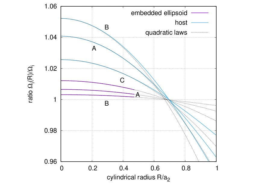
hence . Then, the rotation profiles and are easily deduced from (71) by derivation. We show in Fig. 14 the rotation profile for the embedded spheroid and the host deduced from (71), (72b) and (72a) for configurations A, B and C already considered (see Tabs. 1 and 3). While the range of variation of is of the order of a few purcents (which validates the approximation), we clearly see an underlying quadratic law for , and even a quartic contribution for the host.
Another point that would merit some investigation concerns the dynamical stability of the system. A possible option is to reproduce the present analysis in the case of a two-components, triaxial body (Martinez et al. 1990, e.g.), and to compare the energies between the spheroidal and the ellipsoidal configurations. In this purpose, a dedicated code capable of solving the three dimensional problem numerically, for instance via the SCF-method, seems vital.
Data availability
All data are incorporated into the article.
Acknowledgements
I am grateful to Pr. J. Tohline, Dr. B. Basillais and A. Meunier for advices and suggestions on the article. We thank the anonymous referee for a very detailed examination of the paper and the many suggestions (including a few key-references on classical works) that has enabled to improve the paper.
References
- Abramyan & Kaplan (1974) Abramyan M. G., Kaplan S. A., 1974, Astrophysics, 10, 358
- Abramyan & Kaplan (1975) Abramyan M. G., Kaplan S. A., 1975, Astrophysics, 11, 77
- Amendt et al. (1989) Amendt P., Lanza A., Abramowicz M. A., 1989, ApJ, 343, 437
- Basillais & Huré (2021) Basillais B., Huré J. M., 2021, MNRAS, 506, 3773
- Binney & Tremaine (1987) Binney J., Tremaine S., 1987, Galactic dynamics. Princeton, NJ, Princeton University Press, 1987, 747 p.
- Brosche et al. (1983) Brosche P., Caimmi R., Secco L., 1983, A&A, 125, 338
- Caimmi (1986) Caimmi R., 1986, A&A, 159, 147
- Caimmi (2016) Caimmi R., 2016, Applied Mathematical Sciences, 10, 1821
- Caimmi & Secco (1990) Caimmi R., Secco L., 1990, A&A, 237, 336
- Chandrasekhar (1933) Chandrasekhar S., 1933, MNRAS, 93, 390
- Chandrasekhar (1969) Chandrasekhar S., 1969, Ellipsoidal figures of equilibrium. Yale Univ. Press
- Chandrasekhar & Roberts (1963) Chandrasekhar S., Roberts P. H., 1963, ApJ, 138, 801
- Durisen (1978) Durisen R. H., 1978, ApJ, 224, 826
- Hamy (1889) Hamy M., 1889, Annales de l’Observatoire de Paris, 19, F.1
- Hamy (1890) Hamy M., 1890, Journal de mathématiques pures et appliquées. Tome VI. Gauthier-Villars et Fils
- Huré (2021) Huré J. M., 2021, submitted to MNRAS (Paper II)
- Jeans (1928) Jeans J. H., 1928, Astronomy and cosmogony
- Kadam et al. (2016) Kadam K., Motl P. M., Frank J., Clayton G. C., Marcello D. C., 2016, MNRAS, 462, 2237
- Kelvin et al. (1883) Kelvin W., Tait P., Darwin G., 1883, Treatise on Natural Philosophy. No. vol. 1,ptie. 2 in Treatise on Natural Philosophy, At the University Press
- Kiuchi et al. (2010) Kiuchi K., Nagakura H., Yamada S., 2010, ApJ, 717, 666
- Love et al. (1914) Love A., Appell P., Beghin H., Villat H., 1914, Encyclopédie des sciences mathématiques pures et appliquées. Tome IV. Cinquième volume. Fascicule 2. 18.4. Les grands classiques Gauthier-Villars, J. Gabay, Sceaux
- Lyttleton (1953) Lyttleton R., 1953, The Stability of Rotating Liquid Masses. University Press
- Maeder (1971) Maeder A., 1971, A&A, 14, 351
- Maeder (2009) Maeder A., 2009, Physics, Formation and Evolution of Rotating Stars
- Martinez et al. (1990) Martinez F. J., Cisneros J., Montalvo D., 1990, Rev. Mex. Astron. Astrofis., 20, 15
- Montalvo et al. (1983) Montalvo D., Martinez F. J., Cisneros J., 1983, Rev. Mex. Astron. Astrofis., 5, 293
- Moulton (1916) Moulton E. J., 1916, Transactions of the American Mathematical Society, 17, 100
- Perek (1950) Perek L., 1950, Bulletin of the Astronomical Institutes of Czechoslovakia, 2, 75
- Pohánka (2011) Pohánka V., 2011, Contributions to Geophysics and Geodesy, 41, 117
- Poincaré (1888) Poincaré H., 1888, Comptes rendus des seéances de l’académie des sciences. Tome 106. Gauthier-Villars et Fils
- Ragazzo (2018) Ragazzo C. G., , 2018, The theory of figures of Clairaut with focus on the gravitational rigidity modulus: inequalities and an improvement in the Darwin-Radau equation
- Robe & Leruth (1984) Robe H., Leruth L., 1984, A&A, 133, 369
- Rozelot et al. (2001) Rozelot J. P., Godier S., Lefebvre S., 2001, Sol. Phys., 198, 223
- Rucinski (1988) Rucinski S. M., 1988, AJ, 95, 1895
- Schönberg & Chandrasekhar (1942) Schönberg M., Chandrasekhar S., 1942, ApJ, 96, 161
- Smeyers (1986) Smeyers P., 1986, A&A, 160, 385
- Tassoul (1978) Tassoul J.-L., 1978, Theory of rotating stars
Appendix A The limit of small ellipticities
For and , we can expand the ’s, and subsequently the leading term and the st-order correction . We have
| (75) |
and
| (76) |
According to (26), (42) and (47), we find at point B2
| (77) | ||||
since . In a similar way, we have at point A2
| (78) |
where and is given by (25). This latter relationship can be expanded as
| (79) | ||||
It follows that
| (80) | ||||
Appendix B A basic F90 program
Program nsfoe ! gfortran nsfoe.f90; ./a.out
  Implicit None
  Integer,Parameter::AP=Kind(1.00D+00)
  Real(Kind=AP),Parameter::PI=Atan(1._AP)*4
  Real(Kind=AP)::e12,e1,e1bar,e22,e2,e2bar,q,qe1,c,correction,xa,xb,fa,fb,eprima,eprimb
  Real(Kind=AP)::alpha,alphac,const1,const2,om1over2,om2over2,pif,pc,mass,vol
  ! Statements
  print*,"from J.M.Hur\’e (2021), MNRAS, ’Nested Spheroidal Figures of Equilibrium. I’"
  e2bar=0.3_AP;e1bar=0.75_AP;q=0.2_AP ! configuration F
  e2bar=0.35_AP;e1bar=0.25_AP;q=0.9_AP ! configuration E
  e2bar=0.75_AP;e1bar=0.2_AP;q=0.8_AP ! configuration D
  e2bar=0.90_AP;e1bar=0.95_AP;q=0.45_AP/e1bar;alpha=6.355758519789902_AP ! configuration A
  e22=1._AP-e2bar**2;e2=sqrt(e22);e12=1._AP-e1bar**2;e1=sqrt(e12);qe1=q*e1
  c=qe1**2-e22; print*,"Confocal parameter c",c
  xb=1._AP;eprimb=qe1/Sqrt(xb);fb=q**3*e1bar/xb/sqrt(xb-qe1**2)
  correction=fb*(cteA0(eprimb)-(1._AP-e22)*cteA3(eprimb))
  xa=1._AP+c;eprima=qe1/Sqrt(xa);fa=q**3*e1bar/xa/sqrt(xa-qe1**2)
  correction=correction-fa*(cteA0(eprima)*xa-(1._AP-e22)*cteA3(eprima))
  print*,"1rst-order correction M(e2).f.C|",correction
  pif=cteA0(e2)+(alpha-1._AP)*cteA0(e1)*q**2-(cteA3(e2)+(alpha-1._AP)*cteA3(e1))*e1bar**2*q**2
  pif=pif-(cteA0(e2)+(alpha-1._AP)*fa*cteA0(eprima)*xa)&
      &+(cteA3(e2)+(alpha-1._AP)*fa*cteA3(eprima))*e2bar**2
  pc=pif+alpha*(cteA3(e2)+(alpha-1._AP)*cteA3(e1))*e1bar**2*q**2
  print*,"Interface pressure p*(E1)",pif;print*,"Central pressure",pc
  const1=pc/alpha-(cteA0(e2)+(alpha-1._AP)*cteA0(e1)*q**2)
  const2=-(cteA0(e2)+(alpha-1._AP)*fa*cteA0(eprima)*xa)&
      &+(cteA3(e2)+(alpha-1._AP)*fa*cteA3(eprima))*e2bar**2
  print*,"Const ",const1;print*,"Const’",const2
  alphac=1._AP+(cteM(e2)+cteM(e1)*Pos(e1,e2))/(cteM(e1)+cteM(e2)*fb*Pos(e2,eprimb)+correction)
  om1over2=cteM(e1)*(alphac-1._AP-Pos(e1,e2))
  print*,"TYPE-C SOLUTION";print*," Mass density jump",alphac;print*," Rotation rate W^2",om1over2
  print*,"TYPE-V SOLUTION";print*,"Alpha",alpha
  om2over2=cteM(e2)-(alpha-1._AP)*(fb*cteA0(eprimb)-fa*cteA0(eprima)*(1._AP+c)&
       &+fa*cteA3(eprima)*(1._AP-e22)-fb*cteA1(eprimb))
  om2over2=cteM(e2)*(1._AP-(alpha-1._AP)*fb*Pos(e2,eprimb)-(alpha-1._AP)*correction/cteM(e2))
  om1over2=(om2over2+(alpha-1._AP)*(cteA1(e2)+(alpha-1._AP)*cteA1(e1)&
       &-(cteA3(e2)+(alpha-1._AP)*cteA3(e1))*(1._AP-e12)))/alpha
  print*," Rotation rate W^2 (host)",om2over2;print*," Rotation rate W^2 (embedded ell.)",om1over2
  vol=PI*e2bar*4/3;print*,"Volume",vol;mass=PI*(e2bar+(alpha-1)*q**3*e1bar)*4/3
  print*,"Total mass",mass;print*,"Fractional mass (embedded ell.)",PI*alpha*q**3*e1bar*4/3/mass
Contains
  Function cteA0(e)
    Implicit none;Real(Kind=AP)::e,cteA0
    cteA0=2._AP;If (e>0._AP) cteA0=Sqrt(1._AP-e**2)/e*Asin(e)*2
  End Function cteA0
  Function cteA1(e)
    Implicit none;Real(Kind=AP)::e,cteA1
    cteA1=2._AP/3;If (e>0._AP) cteA1=Sqrt(1._AP-e**2)/e**2*(Asin(e)/e-Sqrt(1._AP-e**2))
  End Function cteA1
  Function cteA3(e)
    Implicit none;Real(Kind=AP)::e,cteA3
    cteA3=2._AP/3;If (e>0._AP) cteA3=Sqrt(1._AP-e**2)/e**2*(1._AP/Sqrt(1._AP-e**2)-Asin(e)/e)*2
  End Function cteA3
  Function cteM(e)
    Implicit none;Real(Kind=AP)::e,cteM
    cteM=0._AP;If (e*(1._AP-e)>0._AP) cteM=cteA1(e)-(1._AP-e**2)*cteA3(e)
  End Function cteM
  Function Pos(x,y)
    Implicit none;Real(Kind=AP)::x,y,Pos
    Pos=-1._AP;If (x*(1._AP-x)>0._AP) Pos=(cteA3(y)*(1._AP-x**2)-cteA1(y))/cteM(x)
  End Function Pos
End Program nsfoe