Learning Dynamics and Structure of Complex Systems Using Graph Neural Networks

A graph neural network (Scarselli et al. 2009; Li et al. 2016; Battaglia et al. 2018) is a message-passing algorithm defined over a graph $\mathcal{G}=(\mathcal{V},\mathcal{E})$ with vertices $\mathcal{V}$ and edges $\mathcal{E}$. For a graph of size $N$, $\mathcal{V}=\{1,\ldots,N\}$ and $\mathcal{E}\subseteq\{(i,j)\mid{(i,j)\in\mathcal{V}^{2}\wedge i\neq j}\}$ where $(i,j)$ represents a directed edge from vertex $j$ to $i$. Each vertex $i$ is associated with a vertex parameter ${\boldsymbol{v}}_{i}$, and each edge $(i,j)$ is associated with an edge parameter ${\boldsymbol{e}}_{ij}$. We assume that all vertex parameters ${\boldsymbol{v}}_{i}$ are of the same dimension $D_{v}$, and all edge parameters ${\boldsymbol{e}}_{ij}$ are of dimension $D_{e}$.

We use GNNs to model observations of a dynamical system at discrete time points. At each time point $t$, vertex $i$ receives a $D_{x}$-dimensional external input ${\boldsymbol{x}}_{i}^{t}$. We take $D_{x}$ to be the same for all vertices, and $D_{x}=0$ represents purely autonomous dynamics of a system. The state of vertex $i$ at time $t$ is denoted as ${\boldsymbol{s}}_{i}^{t}$, which is a vector of dimension $D_{s}$. Vertex states get updated by both time-varying inputs (when $D_{x}>0$) and the lateral interaction from neighboring vertices in the form of messages.

Along the edge $(i,j)$, a pairwise message ${\boldsymbol{m}}_{ij}^{t}$ of dimension $D_{m}$ is generated by a message function $\mathcal{M}(\cdot)$,

where ${\boldsymbol{\Theta}}_{\mathcal{M}}$ is the parameter of $\mathcal{M}(\cdot)$. All incoming messages on vertex $i$ are then aggregated via an aggregation function $\mathcal{A}(\cdot)$,

$\mathcal{A}(\cdot)$ takes the set of pairwise messages as input, ignoring their order, hence it is invariant to permutation. Simple choices of $\mathcal{A}(\cdot)$ include element-wise summation and max pooling, while more complicated mechanisms such as attention-based aggregation can also be used (Veličković et al. 2018; Liao et al. 2019). We choose summation in this study. The vertex state is updated by an update function $\mathcal{U}(\cdot)$,

where ${\boldsymbol{\Theta}}_{\mathcal{U}}$ is the parameter of $\mathcal{U}(\cdot)$. And finally, the GNN output is the projection of states via a readout function $\mathcal{R}(\cdot)$ that applies to every vertex separately,

where ${\boldsymbol{\Theta}}_{\mathcal{R}}$ is the parameter of $\mathcal{R}(\cdot)$.

There is an intrinsic degeneracy among $\mathcal{M}(\cdot)$, $\mathcal{U}(\cdot)$ and $\mathcal{R}(\cdot)$: the complexity of one function may be compensated by the other two. In this study, we use simple linear readouts, so all nonlinearities must be captured by message and update functions. We also assume the readout function $\mathcal{R}(\cdot)$ does not depend on vertex parameters ${\boldsymbol{v}}_{i}$.

A probabilistic graph model (PGM) describes a joint distribution of $N$ random variables $\theta_{1},\ldots,\theta_{N}$. Here we focus on PGMs with pairwise interactions. In a graph of size $N$, each vertex $i$ is associated with a singleton potential $\phi_{i}(\theta_{i})$, and each undirected edge $(i,j)$ is associated with a pairwise potential $\psi_{ij}(\theta_{i},\theta_{j})$. The joint distribution of $\left(\theta_{1},\ldots,\theta_{N}\right)$ is proportional to the product of all potentials,

Marginalization of the joint distribution is one of the most used computation in statistical analysis, and many different methods have been developed for it, including belief propagation (BP), which is an iterative algorithm that operates on a PGM. At each time point $t$, BP estimates the marginal distribution $p_{i}(\theta_{i})$ as $\hat{p}_{i}^{t}(\theta_{i})$. BP is not guaranteed to converge, and even when it converges it is not guaranteed to converge to the true marginal distribution, however it provides a decent estimation in many cases (Murphy et al. 1999; Wainwright et al. 2003).

To make the BP dynamics more interesting, we use time-varying singleton potentials $\phi_{i}^{t}(\theta_{i})$ while keeping the pairwise potential $\psi_{ij}(\theta_{i},\theta_{j})$ constant. This simulates a system with time-varying local evidence while the coupling among different parts is fixed. BP output $\hat{p}_{i}^{t}(x_{i})$ therefore is the continuous estimate of $p_{i}^{t}(\theta_{i})$ determined by $\phi_{i}^{t}(\theta_{i})$ and $\psi_{ij}(\theta_{i},\theta_{j})$.

An important merit of GNN is that the dynamical and structural aspects of a system are represented separately. The canonical functions characterize the dynamics “law” of a certain type of system, such as the BP algorithm, while the graph parameters describe the structure of a particular system instance, e.g. the pairwise coupling in a PGM.

Because both aspects affect the system behavior, it is not trivial to disentangle them based on the observations of the system. In order to inspect the effect of different structures while keeping the dynamics fixed, we need a large number of vertices and edges that cover a wide range of parameters, which suggests using a huge graph. However, training GNN on a huge fully connected graph is computationally expensive. Instead, a more feasible approach is to train multiple medium graphs simultaneously. It is equivalent to training on a huge graph with the knowledge that it is a union of several disconnected components.

In this study, we prepare BP traces on multiple PGMs and simultaneously train multiple GNNs corresponding to each. The GNNs share the same canonical functions but different graph parameters for each individual PGM. The training objective function is simply the summation of loss function over all PGMs (Fig. 1a). Each individual loss is designed to be proportional to the amount of data, therefore the trained canonical functions are naturally biased towards the PGMs with more training data.

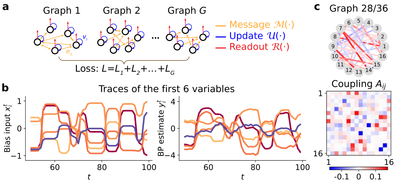
We categorize the GNN parameters as dynamical parameters ${\boldsymbol{\Theta}}^{\mathrm{D}}={\boldsymbol{\Theta}}_{\mathcal{M}}\cup{\boldsymbol{\Theta}}_{\mathcal{U}}\cup{\boldsymbol{\Theta}}_{\mathcal{R}}$ and structural parameters ${\boldsymbol{\Theta}}^{\mathrm{S}}=\{{\boldsymbol{e}}_{ij}\}\cup\{{\boldsymbol{v}}_{i}\}$. Denoting the number of GNN models as $G$, we need to learn one set of shared dynamical parameters ${\boldsymbol{\Theta}}^{\mathrm{D}}$, and $G$ sets of structure parameters ${\boldsymbol{\Theta}}^{\mathrm{S}}_{1},\ldots,{\boldsymbol{\Theta}}^{\mathrm{S}}_{G}$ for each PGM respectively.

We study the BP algorithm on a time-varying multivariate Gaussian distribution defined by

The joint distribution $p({\boldsymbol{\theta}})$ can be rewritten as

with ${\boldsymbol{A}}_{ii}=a_{i},{\boldsymbol{A}}_{ij}={\boldsymbol{A}}_{ji}=J_{ij}$ as the precision matrix. The bias time series ${\boldsymbol{b}}^{t}$ is a sequence of constant values with random duration following a Poisson process, while switching between periods are smoothed by a Hamming window.

Since the marginal distributions $p_{i}(\theta_{i})$ are also Gaussian distributions, BP on Gaussian distribution (Bickson 2009) returns its single-variable means $\mu_{i}^{t}$ and standard deviations $\sigma_{i}^{t}$, i.e.,

When converged, these means are exact but the standard deviations are approximate for loopy graphs (Weiss & Freeman 2001). We use a damped version of the BP algorithm so that belief update is slower, and add processing noise at each time step (). The damping parameter is adjusted so that transient dynamics makes up a significant portion of the full trial. When the precision matrix ${\boldsymbol{A}}$ is constant, the estimated standard deviation $\sigma_{i}^{t}$ quickly converges to the true value $\frac{1}{\sqrt{a_{i}}}$ independent of any time-dependent bias terms, so we focus on $\mu_{i}^{t}$ only. An example trial of BP trace is shown in Fig. 1b.

The inputs to GNN are ${\boldsymbol{x}}_{i}^{t}=[b_{i}^{t}]$, and the targets for the GNN to match are defined as ${\boldsymbol{y}}_{i}^{t}=[\mu_{i}^{t}]$. The GNN output ${\boldsymbol{o}}_{i}^{t}$ (Eq. 4) is constructed to have the same dimension as ${\boldsymbol{y}}_{i}^{t}$, in this case of dimension 1. We use the squared error $L=\sum_{i,t}\|{\boldsymbol{o}}_{i}^{t}-{\boldsymbol{y}}_{i}^{t}\|^{2}$ as the loss function. As introduced in Section 4.1, the losses on all PGMs are summed up as the overall objective function. In practice, each training batch is fetched from a randomly selected PGM. Our loss includes $L_{2}$ regularization on the structural parameters ${\boldsymbol{\Theta}}^{\mathrm{S}}=\{{\boldsymbol{e}}_{ij}\}\cup\{{\boldsymbol{v}}_{i}\}$, which turn out to be critical in disentangling ${\boldsymbol{\Theta}}^{\mathrm{S}}$ from ${\boldsymbol{\Theta}}^{\mathrm{D}}$ (see Section 5.5).

BP traces for 36 random PGMs are generated, using different number of variables, number of trials and time duration for each. The graph density and coupling strengths are approximately the same for all PGMs. More details can be found in Appendix D.

The GNN architecture is determined by various hyper-parameters, including the underlying graph connectivity $\mathcal{E}$, the dimensions $D_{v}$, $D_{e}$, $D_{s}$, $D_{m}$, and hidden layer sizes of canonical functions $\mathcal{M}(\cdot)$ and $\mathcal{U}(\cdot)$. We study the effect of hyper-parameters by performing an extensive search of model configurations and comparing the fitting quality of the trained GNNs. We first define a set of possible values for each hyper-parameter, randomly choose combinations for a GNN architecture, and find the best architecture conditioned on each value to examine the effect of this hyper-parameter. For example, if the candidate values for edge dimension $D_{e}$ are $\{0,2,4,8\}$, the best architectures found by hyper-parameter search conditioned on each $D_{e}$ value are compared.

The graph connectivity $\mathcal{E}$ is treated as a hyper-parameter because it is difficult to learn it in an end-to-end manner. Without any prior knowledge of the structure of a system, the only fair choices are a null graph ($\mathcal{E}=\varnothing$) or a complete graph ($\mathcal{E}=\{(i,j)\mid{(i,j)\in\mathcal{V}^{2}\wedge i\neq j}\}$). The former (‘null’) assumes no coupling among variables, while the latter (‘full’) assumes all pairs of coupling are possible. Not surprisingly, ‘full’ GNNs fit data better than ‘null’ GNNs (Fig. 2a), demonstrating the necessity of pairwise messages for explaining the traces in our BP example. It is worth mentioning that even the ‘null’ GNNs produce good fit ($R^{2}=0.923$), because BP estimates $\mu_{i}^{t}$ in this example are largely determined by the singleton potentials $\phi_{i}(x_{i})$ and only slightly ‘pulled’ by other variables. The reason for using the moderately coupled system is to avoid numerical instability of BP.

We next examine the effects of model component dimensions, including $D_{v}$, $D_{e}$, $D_{s}$ and $D_{m}$. The results (Fig. 2a) show that a non-zero edge dimension is critical in fitting the BP traces on Gaussian distribution; the real coupling is a scalar and thus of dimension 1. Surprisingly, the vertex dimension does not have to be greater than zero, even though the precision parameter $A_{ii}$ is a vertex attribute of dimension 1. We will discuss how to identify ground truth dimension through graph translators in Section 6. There is a small benefit of increasing state dimension $D_{s}$, but no significant effect of message dimension $D_{m}$. It should be noticed that the best architecture for each conditioned value is usually different. For example, the best configuration is $(D_{v}=0,D_{e}=8)$ for $D_{m}=2$ and $(D_{v}=4,D_{v}=1)$ for $D_{m}=12$.

Lastly we examine the effect of message function complexity characterized by the hidden layer sizes in $\mathcal{M}(\cdot)$, and find that nonlinearity in the message is crucial for GNNs to fit well (Fig. 2a). Due to the high cost of hyper-parameter search, we do not compare different update functions, but fix it as a GRU function modulated by the vertex parameter ${\boldsymbol{v}}_{i}$. A more thorough search is left for future work.

To summarize, the results show strong dependency of fitting quality on graph connectivity, edge dimension and the message function nonlinearity, which indicates that in order to fit this dataset well, nonlinear messages between vertices are essential, and the GNN edges need to be parameterized.

One of the best architecture we find uses ‘full’ connectivity, $D_{e}=2,D_{v}=2,D_{h}=12,D_{m}=12$ and a message function with one hidden layer of size 16. After a short initial burn-in period, the outputs of the trained GNNs faithfully reproduce the BP traces on the held-out testing set ($R^{2}=0.988$, Fig. 2b). Not only do the GNN outputs reach the same equilibrium as BP targets within each input period, but the temporal profile at each input switch is also accurate. An example trial is shown in Appendix E (Fig. 8).

We next analyze the states and messages of this well-trained GNN. We gathered these time series from all graphs and performed principal component analysis (PCA) on them. As expected, GNN states and messages only occupy a small portion of the high-dimensional space. The effective dimension of the manifold is defined as $\tilde{D}=\frac{\left(\sum_{i}{\lambda_{i}}\right)^{2}}{\sum_{i}{\lambda_{i}^{2}}}$, where $\lambda_{i}$ denotes the variance of the $i$-th PC. When the state dimension is set to $D_{s}=12$, the effective dimension of state manifold is only $\tilde{D}_{s}\approx 1.74$ (Fig. 3a). We visualize GNN states in 2D and find they are organized by vertices. States at each vertex form its own curved 1D manifold, slightly separated for different vertices (Fig. 3b).

We perform the same analysis on pairwise messages as well. The effective dimension of messages is $\tilde{D}_{m}\approx 3.37$ for message dimension $D_{m}=12$ (Fig. 3c). Different manifolds occupy the message space with different orientations and offsets. Though messages gathered from all edges are not as structured as states, those on individual edges also trace out its own 1D manifold (Fig. 3d). We analyze the dimensionality of aggregated messages ${\boldsymbol{m}}_{i}^{t}$ (Eq. 2) and find they also lie approximately on a 1D manifold specific to each vertex (Appendix F).

With a clearer picture of the GNN states and messages, we next analyze the learned canonical functions $\mathcal{U}(\cdot)$ and $\mathcal{M}(\cdot)$. We take advantage of the fact that the states and messages conditioned on a vertex or an edge approximately lie on a curved 1-D manifold (Section 5.3). Therefore we can project the states or messages on the leading PC for that vertex or edge, and use this projection as a proxy to visualize how these functions depend on their inputs. Although inputs and outputs of $\mathcal{U}(\cdot)$ and $\mathcal{M}(\cdot)$ are vectors, we use scalar proxies as coordinates to plot heat maps of canoncial functions (Fig. 4).

For a GNN vertex with parameter ${\boldsymbol{v}}_{i}$, the update function $\mathcal{U}(\cdot)$ (Eq. 3) is a function of ${\boldsymbol{s}}_{i}^{t}$, ${\boldsymbol{x}}_{i}^{t}$ and ${\boldsymbol{m}}_{i}^{t}$, in which the ${\boldsymbol{m}}_{i}^{t}$ is the aggregated message for vertex $i$ at time $t$. The input ${\boldsymbol{x}}_{i}^{t}$ is the external input, which is simply the local bias $b_{i}^{t}$ in this case. We denote the scalar proxies as $\tilde{s}_{i}^{t}$, $\tilde{s}_{i}^{t+1}$ and $\tilde{m}_{i}^{t}$ respectively. We then focus on the state change $\Delta\tilde{s}_{i}^{t}=\tilde{s}_{i}^{t+1}-\tilde{s}_{i}^{t}$ as a function of ${\boldsymbol{x}}_{i}^{t}$ and $\tilde{m}_{i}^{t}$. Fig. 4a shows one example, in which the state change $\Delta\tilde{s}_{i}^{t}$ is positive when $\tilde{m}_{i}^{t}$ is small and ${\boldsymbol{x}}_{i}^{t}$ is large, and is negative otherwise. Hence $\Delta\tilde{s}_{i}^{t}$ encodes the discrepancy between aggregated message $\tilde{m}_{i}^{t}$ and the external input ${\boldsymbol{x}}_{i}^{t}$. For a GNN edge with parameter ${\boldsymbol{e}}_{ij}$, the message function $\mathcal{M}(\cdot)$ (Eq. 1) is a function of ${\boldsymbol{s}}_{i}^{t}$ and ${\boldsymbol{s}}_{j}^{t}$ that returns ${\boldsymbol{m}}_{ij}^{t}$. Again we denote corresponding scalar proxies as $\tilde{s}_{i}^{t}$, $\tilde{s}_{j}^{t}$ and $\tilde{m}_{ij}^{t}$. It appears that $\tilde{m}_{ij}^{t}$ changes monotonically with either ${\boldsymbol{s}}_{i}^{t}$ or ${\boldsymbol{s}}_{j}^{t}$, while depending mostly on the source vertex state $\tilde{s}_{j}^{t}$ (Fig. 4b).

The structural parameters ${\boldsymbol{\Theta}}^{\mathrm{S}}=\{{\boldsymbol{e}}_{ij}\}\cup\{{\boldsymbol{v}}_{i}\}$ of each individual GNN are learned independently, and they should relate to the true parameters of the corresponding PGMs. In a multivariate Gaussian distribution, a local precision parameter $A_{ii}$ is associated with each variable, and a coupling strength parameter $A_{ij}$ (Eq. 6–8) is associated with each pair of variables. The hypothesis is that there exists a mapping between GNN vertex parameters ${\boldsymbol{v}}_{i}$ and $A_{ii}$, as well as between GNN edge parameters ${\boldsymbol{e}}_{ij}$ and $A_{ij}$. We will learn this mapping between GNN structural parameters and the static attributes of the target nonlinear dynamical system, and term it a ‘graph translator’ because the conversion goes both ways.

Before learning the translators, we first look at the distribution of ${\boldsymbol{v}}_{i}$ and ${\boldsymbol{e}}_{ij}$. Though $D_{v}=D_{e}=2$ in the trained GNN, both vertex parameters and edge parameters approximately form a 1-D manifold. Moreover, locations on the two manifolds are continuously mapped to the corresponding attributes of PGM (Fig. 5).

The explicit structure that emerges in parameter space depends critically on the regularization of structural parameters during training. Such low-dimensional structure does not show up without the $L_{2}$ norm regularization on ${\boldsymbol{v}}_{i}$ and ${\boldsymbol{e}}_{ij}$. Well-trained but unregularized GNNs still give approximately the same good predictions of BP traces, but the effective dimensionality for vertex and edge parameters are very close to their embedding dimensions of $D_{v}$ and $D_{e}$ (Appendix G).

The graph translator we train is simply an MLP with two hidden layers, though it can be any regression model that predicts $A_{ii}$ from ${\boldsymbol{v}}_{i}$ (vertex translator) or $A_{ij}$ from ${\boldsymbol{e}}_{ij}$ (edge translator), or the opposite direction. To quantitatively evaluate graph translators, we divide all $G$ graphs into training, validation and testing sets. Only the original PGM attributes (e.g. $A_{ii}$ and $A_{ij}$) of training and validation graphs will be used to learn the graph translator, and the testing graphs will be used to evaluate how well the translator behaves. The training graphs are used to train the translator directly, and the validation graphs are only used for early stopping. We also assume it is expensive to obtain the original graph attributes (e.g. in neuroscience applications it is laborious to measure synapse strength by patch-clamping experiments), so we use only a subset of the data in training and validation graphs. Specifically, only 80% of the vertices or edges are randomly selected for training the corresponding graph translator. All vertices and edges in the testing graphs are used for evaluation.

The translated local precision $A_{ii}$ and coupling strength $A_{ij}$ both match the ground truth well, with $R^{2}=0.946$ and $R^{2}=0.867$ respectively (Fig. 6a). Recovered coupling matrix $A_{ij}$ looks similar to the ground truth (Fig. 6b), revealing the correct interactions among different random variables. Since we do not enforce any symmetry about GNN edges ${\boldsymbol{e}}_{ij}$, the recovered coupling matrix is not perfectly symmetric. It is straightforward to reveal the underlying structural connectivity between variables by thresholding the coupling strength (Appendix H).

Graph translators can also be used in the reverse direction to directly construct GNN models for a given PGM. The new GNN uses old dynamical parameter ${\boldsymbol{\Theta}}^{\mathrm{D}}$ with the new structural parameter ${\boldsymbol{\Theta}}^{\mathrm{S}}$ translated from precision matrix ${\boldsymbol{A}}$. We compare the constructed GNNs with two control models. The first is the best trained colorless GNN with $D_{v}=D_{e}=0$, i.e. vertices and edges are homogeneous in a graph. Colorless GNNs can be constructed for new PGM directly, without using a graph translator. The second control is the best-trained GNNs with the same parameter dimension as the constructed one, namely the GNNs we obtained earlier for the testing graphs.

The graph parameters of constructed and trained GNNs are close to each other (Fig. 7a). The constructed $\hat{{\boldsymbol{v}}}_{i}$ and $\hat{{\boldsymbol{e}}}_{ij}$ for the testing PGMs are close to the optimal values ${\boldsymbol{v}}^{*}_{i}$ and ${\boldsymbol{e}}^{*}_{ij}$ from the corresponding trained GNNs. Although the strong bias terms ($b_{i}^{t}$) ensure that even disconnected GNNs would capture some amount of the correct marginals, the colorless GNNs match true traces worst, indicating the benefits of parameterized edges. The trained GNNs match true traces best, since they have access to trace data of the new PGM. The translated GNNs, though never trained on these BP traces, can generate credible traces (Fig. 7b).

References

- Bapst et al. (2020) Bapst, V., Keck, T., Grabska-Barwińska, A., Donner, C., Cubuk, E. D., Schoenholz, S. S., Obika, A., Nelson, A. W. R., Back, T., Hassabis, D., and Kohli, P. Unveiling the predictive power of static structure in glassy systems. Nature Physics, 16(4):448–454, 2020. ISSN 1745-2481. doi: 10.1038/s41567-020-0842-8.
- Battaglia et al. (2016) Battaglia, P., Pascanu, R., Lai, M., Jimenez Rezende, D., and kavukcuoglu, k. Interaction networks for learning about objects, relations and physics. In Lee, D. D., Sugiyama, M., Luxburg, U. V., Guyon, I., and Garnett, R. (eds.), Advances in Neural Information Processing Systems 29, pp. 4502–4510. Curran Associates, Inc., 2016.
- Battaglia et al. (2018) Battaglia, P. W., Hamrick, J. B., Bapst, V., Sanchez-Gonzalez, A., Zambaldi, V., Malinowski, M., Tacchetti, A., Raposo, D., Santoro, A., Faulkner, R., Gulcehre, C., Song, F., Ballard, A., Gilmer, J., Dahl, G., Vaswani, A., Allen, K., Nash, C., Langston, V., Dyer, C., Heess, N., Wierstra, D., Kohli, P., Botvinick, M., Vinyals, O., Li, Y., and Pascanu, R. Relational inductive biases, deep learning, and graph networks. ArXiv e-prints, Jun 2018.
- Bickson (2009) Bickson, D. Gaussian belief propagation: theory and application. PhD thesis, The Hebrew University of Jerusalem, Nov 2009.
- Chang et al. (2017) Chang, M., Ullman, T., Torralba, A., and Tenenbaum, J. B. A compositional object-based approach to learning physical dynamics. In 5th International Conference on Learning Representations, ICLR 2017, Toulon, France, April 24-26, 2017, Conference Track Proceedings. OpenReview.net, 2017. URL https://openreview.net/forum?id=Bkab5dqxe.
- Cho et al. (2014) Cho, K., van Merriënboer, B., Gulcehre, C., Bahdanau, D., Bougares, F., Schwenk, H., and Bengio, Y. Learning phrase representations using RNN encoder–decoder for statistical machine translation. In Proceedings of the 2014 Conference on Empirical Methods in Natural Language Processing (EMNLP), pp. 1724–1734. Association for Computational Linguistics, 2014. doi: 10.3115/v1/d14-1179.
- Cranmer et al. (2020) Cranmer, M., Sanchez-Gonzalez, A., Battaglia, P., Xu, R., Cranmer, K., Spergel, D., and Ho, S. Discovering symbolic models from deep learning with inductive biases. arXiv e-prints, June 2020.
- Fei & Pitkow (2021) Fei, Y. and Pitkow, X. Generalization of graph network inferences in higher-order probabilistic graphical models. arXiv preprint arXiv:2107.05729, 2021.
- Garcia Satorras et al. (2019) Garcia Satorras, V., Akata, Z., and Welling, M. Combining generative and discriminative models for hybrid inference. Advances in Neural Information Processing Systems, 32:13825–13835, 2019.
- Gilmer et al. (2017) Gilmer, J., Schoenholz, S. S., Riley, P. F., Vinyals, O., and Dahl, G. E. Neural message passing for quantum chemistry. In Precup, D. and Teh, Y. W. (eds.), Proceedings of the 34th International Conference on Machine Learning, volume 70 of Proceedings of Machine Learning Research, pp. 1263–1272, International Convention Centre, Sydney, Australia, 06–11 Aug 2017. PMLR.
- Kipf et al. (2018) Kipf, T., Fetaya, E., Wang, K.-C., Welling, M., and Zemel, R. Neural relational inference for interacting systems. ArXiv e-prints, February 2018.
- Li et al. (2016) Li, Y., Tarlow, D., Brockschmidt, M., and Zemel, R. Gated graph sequence neural networks. In In Proceedings of the International Conference on Learning Representations, 11 2016.
- Liao et al. (2019) Liao, R., Li, Y., Song, Y., Wang, S., Hamilton, W., Duvenaud, D. K., Urtasun, R., and Zemel, R. Efficient graph generation with graph recurrent attention networks. Advances in Neural Information Processing Systems, 32:4255–4265, 2019.
- Murphy et al. (1999) Murphy, K. P., Weiss, Y., and Jordan, M. I. Loopy belief propagation for approximate inference: An empirical study. In Proceedings of the Fifteenth Conference on Uncertainty in Artificial Intelligence, UAI’99, pp. 467–475, San Francisco, CA, USA, 1999. Morgan Kaufmann Publishers Inc. ISBN 1558606149.
- Qu et al. (2019) Qu, M., Bengio, Y., and Tang, J. GMNN: Graph Markov neural networks. In Chaudhuri, K. and Salakhutdinov, R. (eds.), Proceedings of the 36th International Conference on Machine Learning, volume 97 of Proceedings of Machine Learning Research, pp. 5241–5250. PMLR, 09–15 Jun 2019.
- Sanchez-Gonzalez et al. (2020) Sanchez-Gonzalez, A., Godwin, J., Pfaff, T., Ying, R., Leskovec, J., and Battaglia, P. Learning to simulate complex physics with graph networks. In III, H. D. and Singh, A. (eds.), Proceedings of the 37th International Conference on Machine Learning, volume 119 of Proceedings of Machine Learning Research, pp. 8459–8468. PMLR, 13–18 Jul 2020.
- Scarselli et al. (2009) Scarselli, F., Gori, M., Tsoi, A. C., Hagenbuchner, M., and Monfardini, G. The graph neural network model. IEEE Transactions on Neural Networks, 20(1):61–80, Jan 2009. ISSN 1045-9227. doi: 10.1109/TNN.2008.2005605.
- Veličković et al. (2018) Veličković, P., Cucurull, G., Casanova, A., Romero, A., Liò, P., and Bengio, Y. Graph attention networks. In International Conference on Learning Representations, 2018. URL https://openreview.net/forum?id=rJXMpikCZ.
- Wainwright et al. (2003) Wainwright, M., Jaakkola, T., and Willsky, A. Tree-based reparameterization framework for analysis of sum-product and related algorithms. IEEE Transactions on Information Theory, 49(5):1120–1146, 2003. doi: 10.1109/TIT.2003.810642.
- Watters et al. (2017) Watters, N., Zoran, D., Weber, T., Battaglia, P., Pascanu, R., and Tacchetti, A. Visual interaction networks: Learning a physics simulator from video. In Guyon, I., Luxburg, U. V., Bengio, S., Wallach, H., Fergus, R., Vishwanathan, S., and Garnett, R. (eds.), Advances in Neural Information Processing Systems, volume 30. Curran Associates, Inc., 2017.
- Weiss & Freeman (2001) Weiss, Y. and Freeman, W. T. Correctness of belief propagation in gaussian graphical models of arbitrary topology. Neural computation, 13(10):2173–2200, 2001.
- Ying et al. (2018) Ying, Z., You, J., Morris, C., Ren, X., Hamilton, W., and Leskovec, J. Hierarchical graph representation learning with differentiable pooling. In Bengio, S., Wallach, H., Larochelle, H., Grauman, K., Cesa-Bianchi, N., and Garnett, R. (eds.), Advances in Neural Information Processing Systems, volume 31. Curran Associates, Inc., 2018.
- Yoon et al. (2019) Yoon, K., Liao, R., Xiong, Y., Zhang, L., Fetaya, E., Urtasun, R., Zemel, R., and Pitkow, X. Inference in probabilistic graphical models by graph neural networks. In 2019 53rd Asilomar Conference on Signals, Systems, and Computers, pp. 868–875. IEEE, 2019.
- Zhang et al. (2019) Zhang, Z., Wu, F., and Lee, W. S. Factor graph neural network. arXiv preprint arXiv:1906.00554, 2019.
Appendix A Meta-MLP
We design a family of MLPs organized by meta-parameters, called meta-MLP or mMLP for short. In an original MLP, the input vector is defined as layer 0 activation . sequential perceptrons transform activation from one layer to the next by