Symmetry breaking yields chimeras in two small populations of Kuramoto-type oscillators

Oleksandr Burylko¹, Erik A. Martens^2,3, and Christian Bick^4,5 Affiliation: ¹Institute of Mathematics, National Academy of Sciences of Ukraine, Tereshchenkivska Str. 3, 01024 Kyiv, Ukraine
²Centre for Mathematical Sciences, Lund University, Sölvegatan 18, 221 00 Lund, Sweden
³Chair for Network Dynamics, Center for Advancing Electronics Dresden (cfaed) and Institute for Theoretical Physics, TU Dresden, 01062 Dresden, Germany
⁴Department of Mathematics, Vrije Universiteit Amsterdam, De Boelelaan 1111, Amsterdam, the Netherlands
⁵Department of Mathematics, University of Exeter, Exeter EX4 4QF, United Kingdom

August 11, 2026

Abstract

Despite their simplicity, networks of coupled phase oscillators can give rise to intriguing collective dynamical phenomena. However, the symmetries of globally and identically coupled identical units do not allow solutions where distinct oscillators are frequency-unlocked—a necessary condition for the emergence of chimeras. Thus, forced symmetry breaking is necessary to observe chimera-type solutions. Here, we consider the bifurcations that arise when full permutational symmetry is broken for the network to consist of coupled populations. We consider the smallest possible network composed of four phase oscillators and elucidate the phase space structure, (partial) integrability for some parameter values, and how the bifurcations away from full symmetry lead to frequency-unlocked weak chimera solutions. Since such solutions wind around a torus they must arise in a global bifurcation scenario. Moreover, periodic weak chimeras undergo a period doubling cascade leading to chaos. The resulting chaotic dynamics with distinct frequencies do not rely on amplitude variation and arise in the smallest networks that support chaos.

Networks of coupled oscillators occur in a wide range of systems in biology, medicine and technology. The proper functioning of such systems often relies on the emergence (or absence) of collective modes such as synchronization, where oscillators lock their frequencies and/or phases Strogatz2004; Pikovsky2003—a phenomenon that can be studied in the prominent Kuramoto model of phase oscillators Kuramoto; Acebron2005. Chimeras are symmetry breaking solutions where part of the population synchronizes while the other oscillates incoherently Kuramoto_Battogtokh_2002, even if oscillators are identical. While this phenomenon has received much attention in recent years Panaggio2016; Omelchenko2018, the bifurcations of chimera solutions in finite networks have remained elusive. In physical/mechanical oscillator models, the emergence of chimera states can be related to resonance MartensThutupalli2013; MartensThutupalli2022, and in phase oscillator models to phase lags between oscillators being near $\pm\frac{\pi}{2}$ Ashwin2014a; Martens2016. Here, we analyze a variant of the Kuramoto model with two populations with two phase oscillators near these parameter points. We present a detailed how phase space is organized and elucidate the emergence and bifurcations of chaotic weak chimeras Bick2017; Martens2016; Bick2018.

I Introduction

Coupled phase oscillator networks have been instrumental in understanding collective dynamic phenomena in real-world oscillatory systems Pikovsky2003; Strogatz2004. To understand the dynamics, in many cases it makes sense to assume an idealized system where all nodes are identically connected to all other nodes (such as in the Kuramoto model Kuramoto; Acebron2005) and/or all nodes are identical (for example, in the classical master stability approach Pecora1998). If both of these assumptions are made for a network of $L\in\mathbb{N}$ oscillators, then the resulting dynamical system is $\mathbf{S}_{L}$ -equivariant, where $\mathbf{S}_{L}$ denotes the group of permutations of $L$ symbols. While these systems can still exhibit intriguing dynamics Bick2011; Pikovsky2015a, the symmetry particularly restricts the speed at which the oscillators evolve: For networks of phase oscillators, all nodes have to be frequency-synchronized since oscillators’ phases cannot pass each other Ashwin2014a.

Dynamics where different oscillators evolve at different (asymptotic) frequencies have attracted significant attention in recent years, a phenomenon commonly known as a chimera; see Refs. Panaggio2015; Schoell2016; Omelchenko2018 for reviews. As such solutions/invariant sets are impossible in $\mathbf{S}_{L}$ -symmetric phase oscillator networks, breaking the full permutational symmetry is necessary for frequency unlocked solutions to arise. To break the symmetries, one can for example fix a proper subgroup $H\subset\mathbf{S}_{L}$ and then consider perturbations to the dynamical equations such that the perturbed system is $H$ -equivariant—this is also known as forced symmetry breaking Guyard1999. Breaking the symmetries will break some of the invariant subspaces that restrict the dynamics and create the possibility for frequency-unlocked chimera-type solutions. For example, consider perturbing a network of $L=MN$ oscillators to form $M$ populations of $N$ oscillators each: Let $\theta_{\sigma,k}\in\mathbb{T}:=\mathbb{R}/2\pi\mathbb{Z}$ denote the phase of oscillator $k\in\left\{1,\dotsc,N\right\}$ of population $\sigma\in\left\{1,\dotsc,M\right\}$ . The phase evolves according to

\begin{split}\dot{\theta}_{\sigma,k}:=\frac{\mathrm{d}}{\mathrm{d}t}\theta_{\sigma,k}&=\omega+\frac{1}{MN}\sum_{j=1}^{N}g_{\mathrm{s}}(\theta_{\sigma,j}-\theta_{\sigma,k})\\ &\qquad\quad+\frac{1}{MN}\sum_{\tau\neq\sigma}\sum_{j=1}^{N}g_{\mathrm{n}}(\theta_{\tau,j}-\theta_{\sigma,k}),\end{split}

(1)

where $g_{\mathrm{s}}:\mathbb{T}\to\mathbb{R}$ determines the self-coupling within populations and $g_{\mathrm{n}}:\mathbb{T}\to\mathbb{R}$ determines the coupling to other populations (i.e., ‘neighbors’). The system has a wreath product symmetry $H$ , whose elements act within populations or permute populations Dionne1996a. Note that, by definition, the perturbed system retains the symmetries $H$ ; thus the type of symmetry breaking is different from adding heterogeneity Ashwin2006, which, generically, does not preserve any symmetries. In particular, the populations in (1) are interchangeable in contrast to networks with distinct populations Hong2011a.

Splitting the oscillators into just $M=2$ populations can lead to frequency-unlocked chimera dynamics. Indeed, the classical work by Abrams et al. (Ref. Abrams2008) demonstrated the emergence of chimera solutions for two coupled populations with disparate coupling strength (but identical coupling functions $g_{\mathrm{s}}=g_{\mathrm{n}}$ ) in the limit of $N\to\infty$ oscillators. More generic interactions with nonidentical phase lags and a single harmonic in the limit of large networks may lead to chaotic collective dynamics Martens2016; Bick2018. Chimera solutions not only arise in the mean-field limit but also for finite networks Panaggio2016 and general sinusoidal coupling is sufficient to obtain chaotic dynamics Bick2018. While it was already indicated in Ref. Bick2018 that chaotic dynamics are possible even in the smallest networks of $M=2$ populations of $N=2$ oscillators, the bifurcations that lead to chaotic chimera dynamics remained elusive.

In this paper, we analyze symmetry breaking away from full permutational symmetry to understand the dynamics of small networks of $M=2$ populations of $N=2$ oscillators with generic sinusoidal coupling. This means that while the coupling functions $g_{\mathrm{s}},g_{\mathrm{n}}$ both have a single harmonic, they may have with distinct phase shifts and amplitudes. We first analyze degenerate cases where the dynamical system is either a gradient system or Hamiltonian-like with conserved quantities. These special cases allow to understand how frequency unlocked dynamics arise in these small networks: Perturbing away from the singular parameter values yields global bifurcation scenarios that give rise to frequency-unlocked limit cycle solutions—they correspond to weak chimeras. As such, these solutions have nonzero winding number, wrap around the torus, and have nontrivial homology. How (some of) these solutions bifurcate ¹¹ 1 Note that further branches co-exist. further is shown in the numerical bifurcation diagram in Fig. 1(a): The dynamics eventually undergo a period doubling cascade that leads to chaotic weak chimeras. Finally, we highlight that for certain parameter values, the system has simultaneously conservative and dissipative dynamics in different regions of phase space.

Refer to caption — Figure 1: The road to chaotic weak chimeras. Panel (a) shows a bifurcation diagram obtained via quasi-continuation (see Sec. V.3) for fixed $A=0.7$ and $\alpha_{\mathrm{s}}=0.44$ . Vertical lines delineate $\alpha_{\mathrm{s}}$ -values for the trajectories shown later in Fig. 9, referring to the corresponding panel labels. Panel (b) shows the maximal Lyapunov exponent for varying $(\alpha_{\mathrm{s}},\alpha_{n})$ calculated by numerically integrating from a fixed initial condition for $T=10000$ time units. The dashed line indicates parameter values shown in (a).

The paper is organized as follows. In Sect. II we collect basic information about the governing equations (1), identify invariant subspaces and equilibria, and analyze their linear stability. In Sect. III, we consider the case of pure sine coupling (odd coupling) for which the equations of motion are a gradient system. In Sect. IV, we consider the case of pure cosine coupling (even coupling) that leads to the emergence of conserved quantities; the phase space structure elucidates the emergence or frequency-unlocked solutions corresponding to weak chimeras. Subsequently, in Sect. V we show how these weak chimeras bifurcate. Specifically, we detail the bifurcations in Fig. 1 that lead to the emergence of chaotic dynamics. In Sect. VI, we briefly comment on coexisting conservative dissipative dynamics for combined pure sine/cosine coupling. We conclude with a discussion in the final section.

II From global coupling to coupled populations of Kuramoto oscillators

Before we analyze coupled phase oscillator networks, we briefly recall some notions related to dynamical systems that are equivariant with respect to the action of a group of symmetries. Let $F:\mathbb{X}\to T\mathbb{X}$ be a smooth vector field on $\mathbb{X}$ where $T\mathbb{X}$ denotes the tangent bundle. Suppose that a group $\Gamma$ acts on $\mathbb{X}$ . The vector field $F$ is $\Gamma$ -equivariant if

F(\gamma x)=\hat{\gamma}F(x)

for all $\gamma\in\Gamma$ where $\hat{\gamma}$ is the induced action on the tangent space. A $\Gamma$ -equivariant vector field $F$ defines a $\Gamma$ -equivariant dynamical system

\dot{x}=F(x)

(2)

on $\mathbb{X}$ Golubitsky2002; Field2007a. The group $\Gamma_{x}:=\left\{\,\gamma\in\Gamma\,\left|\;\gamma x=x\right.\right\}$ denotes the stabilizer or isotropy subgroup of $x\in\mathbb{X}$ . While the isotropy subgroup describes the symmetries of a single point, the symmetries of a set $X\subset\mathbb{X}$ are $\Sigma(X):=\left\{\,\gamma\in\Gamma\,\left|\;\gamma X\subset X\right.\right\}$ where $\gamma X=\left\{\,\gamma x\,\left|\;x\in X\right.\right\}$ . If $H\subset\Gamma$ is a subgroup, then the set $\Fix(H):=\left\{\,x\in\mathbb{X}\,\left|\;\gamma x=x\ \forall\gamma\in H\right.\right\}$ is invariant under the flow induced by (2).

II.1 Networks of $L$ oscillators

First consider a network dynamical system (1) with $L\in\mathbb{N}$ phase oscillators. For the remainder of the paper, we will assume that the coupling is of Kuramoto-type as in Ref. Martens2016; Choe2016; Bick2018, i.e., the coupling functions only contain the first harmonic. Specifically, we have $g_{\mathrm{s}}(\phi)=K_{\mathrm{s}}\sin(\phi-\alpha_{\mathrm{s}})$ , $g_{\mathrm{n}}(\phi)=K_{\mathrm{n}}\sin(\phi-\alpha_{\mathrm{n}})$ , where $K_{\mathrm{s}},K_{\mathrm{n}}>0$ are the coupling strengths within and between populations and $\alpha_{\mathrm{s}},\alpha_{\mathrm{n}}\in\mathbb{T}$ the phase lags. By rescaling time we can set $K_{\mathrm{s}}+K_{\mathrm{n}}=1$ without loss of generality and parametrize the coupling strength through the disparity parameter $A:=K_{\mathrm{s}}-K_{\mathrm{n}}$ ; see also Ref. Abrams2008. Note that since the coupling is through phase differences, the system is $\mathbb{T}$ equivariant: There is a continuous $\mathbb{T}$ symmetry where $\gamma\in\mathbb{T}$ acts on the phase space $\mathbb{T}^{L}$ by a common phase shift $\theta_{\sigma,k}\mapsto\theta_{\sigma,k}+\gamma$ to all oscillators.

II.1.1 Globally and identically coupled oscillators

If the coupling within and between populations is identical, that is, $A=0$ ( $K_{\mathrm{s}}=K_{\mathrm{n}}$ ) and $\alpha_{\mathrm{s}}=\alpha_{\mathrm{n}}=:\alpha$ , then we have a globally coupled network of $L=MN$ identical oscillators. Omitting the population index $\sigma$ , write $\theta=(\theta_{1},\dotsc,\theta_{L})$ and the evolution of the phase $\theta_{k}$ of oscillator $k\in\left\{1,\dotsc,L\right\}$ is

\dot{\theta}_{k}=\omega+\frac{1}{L}\sum_{j=1}^{L}\sin(\theta_{j}-\theta_{k}-\alpha).

(3)

The system (3) is $\mathbf{S}_{L}$ -equivariant, where $\mathbf{S}_{L}$ denotes the symmetric group on $L$ symbols which acts on $\mathbb{T}^{L}$ by permuting the oscillator indices. This implies that the sets $\mathcal{P}_{mn}:=\left\{\,\theta\,\left|\;\theta_{m}=\theta_{n}\right.\right\}$ are dynamically invariant as fixed-point sets of the transposition that swaps oscillators $m$ and $n$ . Thus, the dynamics can be reduced to the canonical invariant region

\mathcal{C}=\left\{\theta_{1}<\theta_{2}<\dotsb<\theta_{L}<\theta_{1}+2\pi\right\}

that is bounded by $\mathcal{P}_{nm}$ ; see Refs. Ashwin1992; Ashwin2016 for details. Indeed, since the coupling function only contains a first harmonic, the canonical invariant region is foliated into dynamically invariant sheets on which the dynamics are effectively 2-dimensional Watanabe1994.

The symmetries and type of coupling imply that certain phase configurations are dynamically invariant. The phase configuration

\bm{0}=\left\{\,\theta\,\left|\;\theta_{1}=\theta_{2}=\dotsb=\theta_{L}\right.\right\},

(4)

where all oscillators are phase-synchronized is dynamically invariant as the intersection of all $\mathcal{P}_{mn}$ . Phase synchrony is typically quantified by the Kuramoto order parameter

Z(\theta)=\frac{1}{L}\sum_{j=1}^{L}\exp(i\theta_{j})

(5)

with $i:=\sqrt{-1}$ : We have $\left|Z\right|=1$ if and only if $\theta\in\bm{0}$ . Define the antiphase or incoherent phase configurations as

\mathcal{I}=\left\{\,\theta\,\left|\;Z(\theta)=0\right.\right\}.

(6)

The set $\mathcal{I}$ is dynamically invariant for globally coupled networks and is a union of manifolds (see Ref. Ashwin2016).

The symmetries also constrain the frequencies of the oscillators. For a solution $\theta(t)$ of (3) with initial condition $\theta(0)=\theta^{0}$ define the asymptotic average frequencyBick2015c; Bick2015d as

\Omega_{k}(\theta^{0})=\lim_{T\to\infty}\frac{1}{T}\int_{0}^{T}\dot{\theta}_{k}(t)\,\mathrm{d}t.

(7)

Since the sets $\mathcal{P}_{mn}$ are dynamically invariant, the phase difference between oscillators is bounded. This implies that

\Omega_{m}(\theta^{0})=\Omega_{n}(\theta^{0})

(8)

for all $m,n\in\left\{1,\dotsc,L\right\}$ . Recall that a distinguishing feature of a weak chimera is the separation of frequencies Ashwin2016: A trajectory $\theta(t)$ with initial condition $\theta(0)=\theta^{0}$ converges to a weak chimera if there are distinct $m,n,n^{\prime}$ such that $\Omega_{m}(\theta^{0})\neq\Omega_{n}(\theta^{0})=\Omega_{n^{\prime}}(\theta^{0})$ . Thus, weak chimeras cannot exist in fully symmetric systems.

II.1.2 Breaking full symmetry: $M$ populations of $N$ oscillators

Breaking the symmetry is necessary to observe weak chimeras in a network of phase oscillators: Here, we consider the dynamics (1) of $M$ identical populations of $N$ oscillators each. Recall that $L=MN$ . Write $\theta_{\sigma}=(\theta_{\sigma,1},\dotsc,\theta_{\sigma,N})\in\mathbb{T}^{N}$ for the state of population $\sigma\in\left\{1,\dotsc,M\right\}$ and $\theta=(\theta_{1},\dotsc,\theta_{M})\in\mathbb{T}^{L}$ for the state of the entire network. For the Kuramoto-type coupling we are considering, the phase $\theta_{\sigma,k}$ of oscillator $k$ in population $\sigma$ evolves according to

\begin{split}\dot{\theta}_{\sigma,k}&=\omega+\frac{K_{\mathrm{s}}}{MN}\sum_{j=1}^{N}\sin(\theta_{\sigma,j}-\theta_{\sigma,k}-\alpha_{\mathrm{s}})\\ &\qquad\quad+\frac{K_{\mathrm{n}}}{MN}\sum_{\tau\neq\sigma}\sum_{j=1}^{N}\sin(\theta_{\tau,j}-\theta_{\sigma,k}-\alpha_{\mathrm{n}}).\end{split}

(9)

These equations are $\mathbf{S}_{N}\wr\mathbf{S}_{M}=(\mathbf{S}_{N})^{M}\rtimes\mathbf{S}_{M}\subset\mathbf{S}_{L}$ equivariant where $\rtimes$ denotes a semidirect product. Each copy of $\mathbf{S}_{N}$ acts on $\mathbb{T}^{L}$ by permuting the oscillator indices within a given population $\sigma$ and $\mathbf{S}_{M}$ acts by permuting the populations (i.e., the population indices $\sigma$ ); the symmetries within and between populations do not necessarily commute and hence the semi-direct product.

The system has fewer symmetries than the fully symmetric system. For example—in the notation of the previous section—the sets $\mathcal{P}_{mn}$ are only dynamically invariant if oscillators $m,n$ belong to the same population. Note that the oscillators in each population are still fully symmetric. This implies that for (9) there are invariant sets $\mathcal{P}_{\sigma,mn}:=\left\{\,\theta\,\left|\;\theta_{\sigma,m}=\theta_{\sigma,n}\right.\right\}$ for $m,n\in\left\{1,\dotsc,N\right\}$ and any $\sigma\in\left\{1,\dotsc,M\right\}$ .

The (global) Kuramoto order parameter $Z$ is defined as in (5); it quantifies coherence of all oscillators in the network. Naturally, we also define phase synchrony and incoherence for each population: The (local) Kuramoto order-parameter for population $\sigma$ is

Z_{\sigma}(\theta)=\frac{1}{N}\sum_{j=1}^{N}\exp(i\theta_{\sigma,j})

(10)

and we have $Z=\frac{1}{M}\sum_{\sigma=1}^{M}Z_{\sigma}$ .

II.2 Networks of $4$ oscillators

For the remainder of the section, we consider particular small oscillator networks that consist of $M=2$ populations of $N=2$ oscillators; the network is sketched in Fig. 2(a). In this case, the governing equations (9) read


	$\displaystyle\begin{split}\dot{\theta}_{1,1}&=\omega^{\prime}+\frac{1}{4}\big(K_{\mathrm{s}}\sin{(\theta_{1,2}-\theta_{1,1}-\alpha_{\mathrm{s}})}\\ &\qquad\qquad\qquad+K_{\mathrm{n}}\sin{(\theta_{2,1}-\theta_{1,1}-\alpha_{\mathrm{n}})}\\ &\qquad\qquad\qquad+K_{\mathrm{n}}\sin{(\theta_{2,2}-\theta_{1,1}-\alpha_{\mathrm{n}})}\big)\end{split}$			(11a)
	$\displaystyle\begin{split}\dot{\theta}_{1,2}&=\omega^{\prime}+\frac{1}{4}\big(K_{\mathrm{s}}\sin{(\theta_{1,1}-\theta_{1,2}-\alpha_{\mathrm{s}})}\\ &\qquad\qquad\qquad+K_{\mathrm{n}}\sin{(\theta_{2,1}-\theta_{1,2}-\alpha_{\mathrm{n}})}\\ &\qquad\qquad\qquad+K_{\mathrm{n}}\sin{(\theta_{2,2}-\theta_{1,2}-\alpha_{\mathrm{n}})}\big)\end{split}$			(11b)
	$\displaystyle\begin{split}\dot{\theta}_{2,1}&=\omega^{\prime}+\frac{1}{4}\big(K_{\mathrm{s}}\sin{(\theta_{2,2}-\theta_{2,1}-\alpha_{\mathrm{s}})}\\ &\qquad\qquad\qquad+K_{\mathrm{n}}\sin{(\theta_{1,1}-\theta_{2,1}-\alpha_{\mathrm{n}})}\\ &\qquad\qquad\qquad+K_{\mathrm{n}}\sin{(\theta_{1,2}-\theta_{2,1}-\alpha_{\mathrm{n}})}\big)\end{split}$			(11c)
	$\displaystyle\begin{split}\dot{\theta}_{2,2}&=\omega^{\prime}+\frac{1}{4}\big(K_{\mathrm{s}}\sin{(\theta_{2,1}-\theta_{2,2}-\alpha_{\mathrm{s}})}\\ &\qquad\qquad\qquad+K_{\mathrm{n}}\sin{(\theta_{1,1}-\theta_{2,2}-\alpha_{\mathrm{n}})}\\ &\qquad\qquad\qquad+K_{\mathrm{n}}\sin{(\theta_{1,2}-\theta_{2,2}-\alpha_{\mathrm{n}})}\big)\end{split}$			(11d)

with $\omega^{\prime}=\omega-\frac{K_{\mathrm{s}}}{4}\sin\alpha_{\mathrm{s}}$ . If the coupling is fully symmetric, i.e., $K_{\mathrm{s}}=K_{\mathrm{n}}$ and $\alpha_{\mathrm{s}}=\alpha_{\mathrm{n}}$ , then (11) is $\mathbf{S}_{4}$ -equivariant. That means that up to the rotational symmetry, the canonical invariant region is a tetrahedron bounded by the dynamically invariant $\mathcal{P}_{mn}$ (as in Sect. II.1.1); see Refs. Burylko-Pikovsky; Ashwin2016 for details. The phase configuration $\bm{0}$ with full phase synchrony corresponds to each of the four corners of the tetrahedron. The incoherent phase configurations $\mathcal{I}$ in $\mathcal{C}$ are the points with $\mathbf{S}_{2}\times\mathbf{S}_{2}$ isotropy, that is, a line of points parametrized by $(a,b,a+\pi,b+\pi)\in\mathbb{T}^{4}$ .

For a generic choice of coupling parameters, the dynamical system (11) is $\mathbf{S}_{2}\wr\mathbf{S}_{2}\equiv\mathbf{D}_{4}$ -equivariant, the symmetries of the square; cf. Fig. 2(a). Specifically, $\mathbf{D}_{4}$ is generated by the rotational symmetry


	$\displaystyle\overline{\gamma}_{\mathrm{r}}$	$\displaystyle:(\theta_{1,1},\theta_{1,2},\theta_{2,1},\theta_{2,2})\mapsto(\theta_{2,2},\theta_{2,1},\theta_{1,1},\theta_{1,2}),$	(12a)
(a clockwise rotation by an angele of $\frac{\pi}{2}$ in Fig. 2(a)) and the mirror symmetry
	$\displaystyle\overline{\gamma}_{\mathrm{m}}$	$\displaystyle:(\theta_{1,1},\theta_{1,2},\theta_{2,1},\theta_{2,2})\mapsto(\theta_{1,1},\theta_{1,2},\theta_{2,2},\theta_{2,1})$	(12b)

(a flip about the main diagonal in Fig. 2(a)). General properties of $\mathbf{D}_{4}$ -equivariant phase oscillator networks can be found in Ref. Ashwin1992. The codimension-1 invariant subspaces are $\mathcal{P}_{1,12}=\left\{\theta_{1,1}=\theta_{1,2}\right\}$ and $\mathcal{P}_{2,12}=\left\{\theta_{2,1}=\theta_{2,2}\right\}$ . Since we only have two oscillators per population we will write $\mathcal{P}_{1}:=\mathcal{P}_{1,12}$ , $\mathcal{P}_{2}:=\mathcal{P}_{2,12}$ for simplicity.

Three values of the disparity parameter stand out where the network structure is qualitatively different. As already discussed, $A=0$ corresponds to $K_{\mathrm{n}}=K_{\mathrm{s}}$ , that is the strength of interactions within and between populations is the same. If in addition also $\alpha_{\mathrm{n}}=\alpha_{\mathrm{s}}$ , the oscillators have full permutational symmetry and we have the Kuramoto–Sakaguchi equations for identical oscillators. If $A=1$ , we have $K_{\mathrm{n}}=0$ and the populations are uncoupled; this means that the green links are absent in Fig. 2(a). If $A=-1$ , we have $K_{\mathrm{s}}=0$ and the oscillators within populations are uncoupled. This configuration is equivalent to a ring of oscillators with nearest-neighbor coupling as illustrated in Fig. 2(a): If the purple links are absent, for a given oscillator the two oscillators of the other population are the direct neighbors.

II.2.1 Reduced Dynamics and Symmetries

The phase-shift symmetry of (11) means that the system dynamics is effectively three-dimensional. We exploit this by rewriting the system in terms of phase differences $\psi_{1}:=\theta_{1,1}-\theta_{1,2},\psi_{2}:=\theta_{1,2}-\theta_{2,1},\psi_{3}:=\theta_{2,1}-\theta_{2,2}$ . This yields the reduced system


	$\displaystyle\begin{split}\dot{\psi}_{1}&=-\frac{K_{\mathrm{s}}}{2}\cos(\alpha_{\mathrm{s}})\sin(\psi_{1})+\frac{K_{\mathrm{n}}}{4}\Big(\sin(\alpha_{\mathrm{n}}+\psi_{2})\\ &\qquad-\sin(\alpha_{\mathrm{n}}+\psi_{1}+\psi_{2})+\sin(\alpha_{\mathrm{n}}+\psi_{2}+\psi_{3})\\ &\qquad-\sin(\alpha_{\mathrm{n}}+\psi_{1}+\psi_{2}+\psi_{3})\Big)\\ \end{split}$			(13a)
	$\displaystyle\begin{split}\dot{\psi}_{2}&=\frac{K_{\mathrm{s}}}{4}\big(\sin(\alpha_{\mathrm{s}}+\psi_{3})-\sin(\alpha_{\mathrm{s}}-\psi_{1})\big)\\ &\qquad+\frac{K_{\mathrm{n}}}{4}\Big(\sin(\alpha_{\mathrm{n}}-\psi_{1}-\psi_{2})\\ &\qquad{-2}\cos(\alpha_{\mathrm{n}})\sin(\psi_{2})-\sin(\alpha_{\mathrm{n}}+\psi_{2}+\psi_{3})\Big)\\ \end{split}$			(13b)
	$\displaystyle\begin{split}\dot{\psi}_{3}&=-\frac{K_{\mathrm{s}}}{2}\cos(\alpha_{\mathrm{s}})\sin(\psi_{3})+\frac{K_{\mathrm{n}}}{4}\Big(-\sin(\alpha_{\mathrm{n}}-\psi_{2})\\ &\qquad-\sin(\alpha_{\mathrm{n}}-\psi_{1}-\psi_{2})+\sin(\alpha_{\mathrm{n}}-\psi_{2}-\psi_{3})\\ &\qquad+\sin(\alpha_{\mathrm{n}}-\psi_{1}-\psi_{2}-\psi_{3})\Big).\\ \end{split}$			(13c)

If the coupling is fully symmetric, i.e., $A=0$ ( $K_{\mathrm{s}}=K_{\mathrm{n}}$ ) and $\alpha_{\mathrm{s}}=\alpha_{\mathrm{n}}$ , then the phase space is organized by invariant planes $\mathcal{P}_{nm}$ , the canonical invariant region, and its images under the symmetry. In the reduced system (13), these invariant planes are given by $\psi_{1}=0$ , $\psi_{3}=0$ , $\psi_{2}=0$ , $\psi_{1}+\psi_{2}=0$ , $\psi_{2}+\psi_{3}=0$ , $\psi_{1}+\psi_{2}+\psi_{3}=0$ , which split $\mathbb{T}^{3}$ into six dynamically invariant regions, the canonical invariant regions and its images. The geometry is illustrated in Fig. 3(a) where one invariant region is bounded by coordinate planes and a light grey plane $\psi_{3}=2\pi-\psi_{1}-\psi_{2}$ . The intersection of all planes correspond to full phase synchrony. As defined above, the set of incoherent phase configurations are the points where the (global) Kuramoto order vanishes; in phase-difference coordinates these are given by

\mathcal{I}=\left\{\,(\psi_{1},\psi_{2},\psi_{3})\,\left|\;e^{i\psi_{1}}+e^{i(\psi_{1}+\psi_{2})}+e^{i(\psi_{1}+\psi_{2}+\psi_{3})}=-1\right.\right\}.

For arbitrary parameters $\alpha_{\mathrm{s}}$ , $\alpha_{\mathrm{n}}$ , $A$ , the network (11) has dihedral symmetry $\mathbf{S}_{2}\wr\mathbf{S}_{2}\equiv\mathbf{D}_{4}$ . In phase differences (13), the generators of the symmetry action (12) are

	$\displaystyle\gamma_{\mathrm{r}}:(\psi_{1},\psi_{2},\psi_{3})$	$\displaystyle\mapsto(-\psi_{3},-\psi_{1}-\psi_{2},\psi_{1}),$		(14)
	$\displaystyle\gamma_{\mathrm{m}}:(\psi_{1},\psi_{2},\psi_{3})$	$\displaystyle\mapsto(\psi_{1},\psi_{2}+\psi_{3},-\psi_{3})$		(15)

that correspond to the rotation and reflection mentioned above. Solutions transform in a nontrivial way along variable $\psi_{2}$ that describes the state of the two populations relative to one another under $\gamma_{\mathrm{r}}$ , $\gamma_{\mathrm{m}}$ . The system also has parameter symmetries

$\displaystyle\gamma^{(-)}$	$\displaystyle:(\psi_{1},\psi_{2},\psi_{3},\alpha_{\mathrm{s}},\alpha_{\mathrm{n}})\mapsto-(\psi_{1},\psi_{2},\psi_{3},\alpha_{\mathrm{s}},\alpha_{\mathrm{n}}),$	(16)
$\displaystyle\gamma^{(\alpha_{\mathrm{n}})}$	$\displaystyle:(\psi_{2};\alpha_{\mathrm{n}})\mapsto(\psi_{2}+\pi;\alpha_{\mathrm{n}}+\pi),$	(17)
$\displaystyle\gamma^{(A,t)}$	$\displaystyle:(\psi_{2};A,t)\mapsto\begin{cases}(\psi_{2}+\pi;1/A,t),&A>0\\ (\psi_{2}+\pi;1/A,-t),&A<0\end{cases}$	(18)

where (18) is time-reversing for $A<0$ .

II.2.2 Equilibria, invariant subspaces, and linear stability

The four oscillator network (13) supports phase-synchronized (or coherent) solutions. Specifically, there are fixed points

	$\displaystyle\bm{0}$	$\displaystyle=(0,0,0),$		(19)
	$\displaystyle\bm{\pi}$	$\displaystyle=(0,\pi,0).$		(20)

The first fixed point corresponds to the phase configuration where all oscillators are in-phase (the point of full isotropy where all phases are equal). The second corresponds to the configuration where both populations are in-phase but anti-phase with respect to each other. Linear stability of the solutions $\bm{0}$ and $\bm{\pi}$ is determined by the eigenvalues


$\displaystyle\lambda_{1}$	$\displaystyle=\mp{K_{\mathrm{n}}}\cos{\alpha_{\mathrm{n}}}$	(21a)
$\displaystyle\lambda_{2}$	$\displaystyle=\mp{\frac{1}{2}}K_{\mathrm{n}}\cos{\alpha_{\mathrm{n}}}-{\frac{1}{2}}K_{\mathrm{s}}\cos{\alpha_{\mathrm{s}}}$	(21b)
$\displaystyle\lambda_{3}$	$\displaystyle=\mp{\frac{1}{2}}K_{\mathrm{n}}\cos{\alpha_{\mathrm{n}}}-{\frac{1}{2}}K_{\mathrm{s}}\cos{\alpha_{\mathrm{s}}}.\$	(21c)

respectively; the signs are for $\bm{0}$ and $\bm{\pi}$ , respectively.

The incoherent phase configurations in $\mathcal{I}$ can be parametrized as three lines


$\displaystyle\mathcal{I}_{0}$	$\displaystyle:=\left\{\,(\pi,\varphi,\pi)\,\left\|\;\varphi\in\mathbb{T}\right.\right\}$	(22a)
$\displaystyle\mathcal{I}_{1}$	$\displaystyle:=\left\{\,(\varphi,\pi-\varphi,\varphi)\,\left\|\;\varphi\in\mathbb{T}\right.\right\}$	(22b)
$\displaystyle\mathcal{I}_{2}$	$\displaystyle:=\left\{\,(\varphi,\pi,-\varphi)\,\left\|\;\varphi\in\mathbb{T}\right.\right\},$	(22c)

such that $\mathcal{I}=\mathcal{I}_{0}\cup\mathcal{I}_{1}\cup\mathcal{I}_{2}$ . The set $\mathcal{I}_{0}$ are the phase configurations where each population is incoherent (that is, the phase difference of the two oscillators is $\pi$ ), the sets $\mathcal{I}_{1}$ and $\mathcal{I}_{2}$ correspond to phase configurations where oscillators in distinct populations have a phase difference of $\pi$ .

The line $\mathcal{I}_{0}$ is a continuum of equilibria. Linearizing the equations, we obtain that linear stability is determined by the eigenvalues


$\displaystyle\lambda_{1}$	$\displaystyle=0$	(23a)
$\displaystyle\lambda_{2}$	$\displaystyle={\frac{1}{2}}K_{\mathrm{s}}\cos\left(\alpha_{\mathrm{s}}\right)-\frac{\|K_{\mathrm{n}}\|}{{2}\sqrt{2}}\sqrt{\cos\left(2\alpha_{\mathrm{n}}\right)+\cos(2\varphi)}$	(23b)
$\displaystyle\lambda_{3}$	$\displaystyle={\frac{1}{2}}K_{\mathrm{s}}\cos\left(\alpha_{\mathrm{s}}\right)+\frac{\|K_{\mathrm{n}}\|}{{2}\sqrt{2}}\sqrt{\cos\left(2\alpha_{\mathrm{n}}\right)+\cos(2\varphi)}\$	(23c)

Writing $a=\frac{K_{\mathrm{s}}}{4}\cos\alpha_{\mathrm{s}}$ , $b=\frac{K_{\mathrm{n}}}{4}\cos(\alpha_{\mathrm{n}}+\varphi)$ , $c=\frac{K_{\mathrm{n}}}{4}\cos(\alpha_{\mathrm{n}}-\varphi)$ we have that $\lambda_{2,3}=2(a\mp\sqrt{bc})$ . This yields the linear stability properties of the equilibria: Phase configurations in $\mathcal{I}_{0}$ are linearly stable if $a<0$ and $bc<a^{2}$ or if $a<\min\{0,\ -\sqrt{bc}\}$ . How the equilibria bifurcate depends on $\varphi$ : The eigenvalues (23) are a complex conjugated pair if $\varphi\in(|\alpha_{\mathrm{n}}-\frac{\pi}{2}|-\pi,-|\alpha_{\mathrm{n}}-\frac{\pi}{2}|)\cup(|\alpha_{\mathrm{n}}-\frac{\pi}{2}|,\pi-|\alpha_{\mathrm{n}}-\frac{\pi}{2}|),$ which suggests a (degenerate) Hopf bifurcation for $K_{\mathrm{s}}\cos\alpha_{\mathrm{s}}=0$ . For other $\varphi$ , the eigenvalues are real. In the limiting case of global coupling ( $K_{\mathrm{s}}=K_{\mathrm{n}}:=1$ , $\alpha_{\mathrm{s}}=\alpha_{\mathrm{n}}=\alpha$ ) the eigenvalues evaluate to

\displaystyle\lambda_{2,3}

\displaystyle=\frac{1}{2}\left(\cos\alpha\mp\sqrt{\cos^{2}\alpha-\sin^{2}\varphi}\right).

Now consider the incoherent phase configurations $\mathcal{I}_{1}$ and $\mathcal{I}_{2}$ . These are invariant lines of (13) for any parameter values. The dynamics on each of these lines is given by

\dot{\varphi}=\frac{1}{2}(K_{\mathrm{n}}\cos(\alpha_{\mathrm{n}})-K_{\mathrm{s}}\cos(\alpha_{\mathrm{s}}))\sin(\varphi).

Thus, $\mathcal{I}_{1}$ and $\mathcal{I}_{2}$ are continua of nonisolated fixed points if $\alpha_{\mathrm{s}}=\alpha_{\mathrm{n}}=\pm\frac{\pi}{2}$ as in the traditional Kuramoto–Sakaguchi equations. Linear stability of these fixed points for $\alpha_{\mathrm{s}}=\alpha_{\mathrm{n}}=\alpha=\pm\frac{\pi}{2}$ is determined by the nontrivial eigenvalues

\lambda_{2,3}=\pm i\frac{1}{2}\sqrt{K_{\mathrm{s}}K_{\mathrm{n}}}\sin(\varphi).

This implies that the set of incoherent phase configurations $\mathcal{I}=\mathcal{I}_{0}\cup\mathcal{I}_{1}\cup\mathcal{I}_{2}$ are surrounded by sets of periodic orbits when $\alpha=\pm\frac{\pi}{2}$ when $K_{\mathrm{n}}K_{\mathrm{s}}>0$ ( $|A|<1$ ). If $\alpha_{\mathrm{s}},\alpha_{\mathrm{n}}\approx\pm\frac{\pi}{2}$ the invariant lines persist and are surrounded by spiral trajectories.

Finally, we consider the set of two-cluster synchronized phase configurations $\mathcal{S}$ , which are the points $\mathbf{S}_{2}\times\mathbf{S}_{2}$ isotropy in the globally coupled system: These are the points where there are two clusters of two oscillators each. In phase difference coordinates on $\mathbb{T}^{3}$ for (13), we define

	$\displaystyle\mathcal{S}_{0}$	$\displaystyle:=\left\{\,(0,\varphi,0)\in\mathbb{T}^{3}\,\left\|\;\varphi\in\mathbb{T}\right.\right\},$
	$\displaystyle\mathcal{S}_{1}$	$\displaystyle:=\left\{\,(\varphi,0,-\varphi)\in\mathbb{T}^{3}\,\left\|\;\varphi\in\mathbb{T}\right.\right\},$
	$\displaystyle\mathcal{S}_{2}$	$\displaystyle:=\left\{\,(\varphi,-\varphi,\varphi)\in\mathbb{T}^{3}\,\left\|\;\varphi\in\mathbb{T}\right.\right\}.$

and have $\mathcal{S}=\mathcal{S}_{0}\cup\mathcal{S}_{1}\cup\mathcal{S}_{2}$ . The set $\mathcal{S}_{0}$ consists of the phase configurations where each of the populations is phase synchronized—this means that $\mathcal{S}_{0}=\mathcal{P}_{1}\cap\mathcal{P}_{2}=\left\{\psi_{1}=0\right\}\cap\left\{\psi_{3}=0\right\}$ ; cf. Fig. 3. The sets $\mathcal{S}_{1},\mathcal{S}_{2}$ are phase configurations where two oscillators of distinct populations are phase-synchronized. The set $\mathcal{S}_{0}$ is dynamically invariant for any values of $\alpha_{\mathrm{s}}$ , $\alpha_{\mathrm{n}}$ , and $A$ as fixed point sets of a subgroup of $\mathbf{D}_{4}$ ; the other two sets are only invariant for certain values of the coupling parameters as we will discuss below. Now the dynamics on $\mathcal{S}_{0}$ is are determined by

\dot{\varphi}=-K_{\mathrm{n}}\cos(\alpha_{\mathrm{n}})\sin(\varphi).

For $\alpha_{\mathrm{n}}\neq\pm\frac{\pi}{2}$ there are exactly two fixed points on this line that correspond to $\bm{0}$ and $\bm{\pi}$ , respectively. For $\alpha_{\mathrm{n}}=\pm\frac{\pi}{2}$ , the set $\mathcal{S}_{0}$ is a continuum of fixed points. Linearization yields the eigenvalues

	$\displaystyle\lambda_{1}$	$\displaystyle=-K_{\mathrm{n}}\cos(\alpha_{\mathrm{n}})\cos(\varphi),$
	$\displaystyle\lambda_{2,3}$	$\displaystyle=-\frac{1}{2}K_{\mathrm{n}}\cos(\alpha_{\mathrm{n}}\mp\varphi)-\frac{1}{2}K_{\mathrm{s}}\cos(\alpha_{\mathrm{s}}).$

Note that the invariant planes $\mathcal{P}_{1}=\left\{\psi_{1}=0\right\}$ and $\mathcal{P}_{2}=\left\{\psi_{3}=0\right\}$ bound the phase differences within each population. Thus, $\Omega_{11,12}=0$ and $\Omega_{21,22}=0$ . By contrast, the phase difference $\psi_{2}$ between the two populations may not be bounded—this corresponds to weak chimeras. In the following sections we will elucidate the dynamical mechanisms that lead to such solutions.

III Gradient dynamics for odd coupling

If the coupling function is a pure sine function ( $\alpha_{\mathrm{s}}=\alpha_{\mathrm{n}}=0$ ), the system (11) is a gradient system²² 2 Note that the dynamics $\alpha_{\mathrm{s}}=\alpha_{\mathrm{n}}=\pi$ are identical up to a sign change.. More precisely, with the potential

	$\displaystyle V(\theta)$	$\displaystyle=-\frac{K_{\mathrm{s}}}{4}(\cos(\theta_{1,1}-\theta_{1,2})+\cos(\theta_{2,1}-\theta_{2,2}))$
		$\displaystyle\qquad-\frac{K_{\mathrm{n}}}{4}\Big(\cos(\theta_{1,1}-\theta_{2,1})+\cos(\theta_{1,1}-\theta_{2,2})$
		$\displaystyle\qquad\qquad\quad+\cos(\theta_{1,2}-\theta_{2,1})+\cos(\theta_{1,2}-\theta_{2,2})\Big),$

equation (11) can be written as

\displaystyle\dot{\theta}_{\sigma,k}=\omega-\frac{\partial}{\partial\theta_{\sigma,k}}V(\theta)

(24)

for $\sigma,k\in\left\{1,2\right\}$ . The system has a parameter symmetry given by the action of $\gamma^{(A)}$ as defined in (18). This allows to restrict the parameter range to $A\in(-1,1)$ and makes the bifurcation behavior of the system for the special parameter values $A=\pm 1$ (corresponding to uncoupled populations and a ring topology, respectively) more transparent. Note that for these parameter values $\gamma^{(-)}$ is an additional $\mathbb{Z}_{2}$ -symmetry.

III.1 Equilibria and their stability

We first analyze the equilibria and their stability for $\alpha_{\mathrm{s}}=\alpha_{\mathrm{n}}=0$ . According to (21), the stability of the coherent equilibrium $\bm{0}$ is determined by the eigenvalues $\lambda_{1}=(A-1)/2,$ $\lambda_{2,3}=-1/2.$ Thus, $\bm{0}$ is an attractor for $A<1$ and a saddle equilibrium otherwise. Similarly, the stability of the equilibrium $\bm{\pi}$ is determined by $\lambda_{1}=(1-A)/2,$ $\lambda_{2,3}=-A/2$ . Thus, $\bm{\pi}$ is a source for $A\leq 0$ , a saddle for $A\in(0,1)$ , and a sink for $A\geq 1$ (with neutral linear stability along $\mathcal{I}_{0}$ for $A=1$ ). Finally, the linearization of the vector field at the incoherent invariant line $\mathcal{I}_{0}=\left\{\,(\pi,\varphi,\pi)\,\left|\;\varphi\in\mathbb{T}\right.\right\}$ has eigenvalues (23), which evaluate to

\displaystyle\lambda_{1}

\displaystyle=0,

\displaystyle\lambda_{2,3}

\displaystyle=\frac{1}{4}(1+A\pm|1-A||\cos(\varphi)|).

Therefore, different points $\mathcal{I}_{0}$ have different transverse stability for certain values of the parameter $A$ . Specifically, for $A<-1$ the equilibria $(\pi,\varphi,\pi)$ are stable if

\displaystyle\varphi

\displaystyle\in(-\varphi^{*},\varphi^{*}-\pi)\cup(\pi-\varphi^{*},\varphi^{*}),

where $\varphi^{*}=\arccos\!\big(\frac{1+A}{|1-A|}\big).$ Decreasing $A$ from zero, the equilibria on $\mathcal{I}_{0}$ are (transversely) stable around $\varphi=\pm\frac{\pi}{2}$ ; the part of $\mathcal{I}_{0}$ with transverse stability increases as $A$ is decreased. Thus, there is multistability of the equilibrium $\bm{0}$ and segments of the manifold $\mathcal{I}_{0}$ if $A<-1$ . Conversely, for $A\in(-1,0)$ equilibria on $\mathcal{I}_{0}$ are repellers if $\varphi\in(\varphi^{*}-\pi,-\varphi^{*})\cup(\varphi^{*},\pi-\varphi^{*})$ . For $A>0$ , the entire line $\mathcal{I}_{0}$ is repelling. In all other cases, the points of $\mathcal{I}_{0}$ are of saddle type.

The system has a number of equilibria for apart from $\bm{0},\bm{\pi}$ , and the continuum $\mathcal{I}_{0}$ . First, the points $(\pi,0,0)$ , $(0,0,\pi)$ , $(\pi,\pi,0)$ , and $(0,\pi,\pi)$ —two cluster configurations of one and three oscillators; cf. Fig. 2(k,l)—are equilibria for any $A$ when $\alpha_{\mathrm{s}}=\alpha_{\mathrm{n}}=0$ . Linear stability is determined by the eigenvalues

\displaystyle\lambda_{1}

\displaystyle=-\frac{K_{\mathrm{s}}}{2},

\displaystyle\lambda_{2,3}

\displaystyle=\frac{1}{4}\left(K_{\mathrm{s}}\pm\sqrt{K_{\mathrm{s}}^{2}+8K_{\mathrm{n}}^{2}}\right).

These equilibria are of saddle type since $K_{\mathrm{n}}>0$ implies $\lambda_{1}\lambda_{2}<0$ , $K_{\mathrm{n}}<0$ implies $\lambda_{1}\lambda_{3}<0$ , and $K_{\mathrm{n}}=0$ implies $\lambda_{2}\lambda_{3}<0$ .

Second, for $A>0$ the system has four symmetric equilibria $(-2\psi^{*},\psi^{*},0)$ , $(2\psi^{*},-\psi^{*},0)$ , $(0,\psi^{*},-2\psi^{*})$ , and $(0,-\psi^{*},2\psi^{*})$ with $\psi^{*}=\arccos\left(\frac{A-1}{A+1}\right)$ . These equilibria are of saddle type and move along a straight line as the parameter $A$ is varied. Pairs of these saddle points (in each plane $\psi_{1}=0$ , $\psi_{3}=0$ ) disappear in pitchfork bifurcations with $\bm{\pi}$ at $A=0$ .

III.2 Bifurcations and integrability

The system bifurcates at $A=-1$ , $A=0$ , and $A=1$ . In each of these cases, the dynamics have additional symmetries and there can be conserved quantities.

If $A=0$ the system is fully symmetric and the well-known Kuramoto model for identical oscillators. The system has a global attractor $\bm{0}$ and repellers $\mathcal{I}=\mathcal{I}_{0}\cup\mathcal{I}_{1}\cup\mathcal{I}_{2}$ consisting entirely of equilibria. Other equilibria with phase difference coordinates $0$ and $\pi$ are saddles in this case. breaking the full permutational symmetry for $A\neq 0$ leads to the disappearance of fixed points from invariant varieties $\mathcal{I}_{1}$ and $\mathcal{I}_{2}$ but these lines remain invariant.

For $A=\pm 1$ the system has conserved quantities. If $A=1$ , the oscillator populations are uncoupled and there is a conserved quantity. A straightforward calculation confirms:

Proposition 1.

For $A=1$ and any $\alpha_{\mathrm{s}},\alpha_{\mathrm{n}}$ (thus also for $\alpha_{\mathrm{s}}=\alpha_{\mathrm{n}}=0$ ) the system has a first integral

H^{(1,\,\cdot\,)}(\psi_{1},\psi_{3})=\cot\!\left(\frac{\psi_{1}}{2}\right)\tan\!\left(\frac{\psi_{3}}{2}\right).

Moreover for the specific gradient cases, we have an additional constant of motion; thus trajectories are completely determined.

Proposition 2.

For $A=1$ and $\alpha_{\mathrm{s}}=0$ the system has a first integral

\displaystyle{H}^{(1,0)}(\psi_{1},\psi_{2},\psi_{3})

\displaystyle=\psi_{1}+2\psi_{2}+\psi_{3}

(25)

If $A=-1$ there is no coupling between distinct populations and we have a network of identical Kuramoto oscillators on a ring. This system also has a conserved quantity.

Proposition 3.

For $A=-1$ and $\alpha_{\mathrm{s}}=\alpha_{\mathrm{n}}=0$ the system has a first integral

{H}^{(-1,0)}(\psi_{1},\psi_{3})=\cot\!\left(\frac{\psi_{1}+\psi_{3}}{4}\right)\tan\!\left(\frac{\psi_{1}-\psi_{3}}{4}\right)

(26)

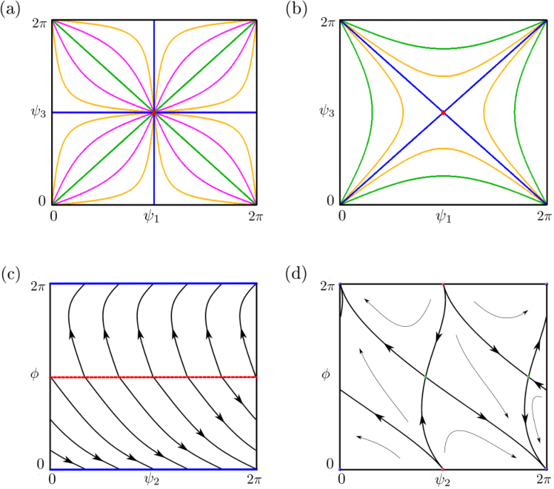
Note that the constant of motion $H^{(1,\cdot)}$ , $H^{(-1,0)}$ do not depend on the inter population phase difference $\psi_{2}$ . Thus, all solutions belong to cylinder-like surfaces. Figure 4 shows the projections of surfaces determined by $H^{(1,\cdot)}(\psi_{1},\psi_{3})=C$ and $H^{(-1,0)}(\psi_{1},\psi_{3})=C$ for fixed $C\in[-1,1]$ onto the plane $(\psi_{1},\psi_{3})$ for different values of parameter $C$ . In addition, for $A=1$ all solutions of the system belong to the parallel planes ${H}^{(1,0)}=\beta$ , $\beta\in\mathbb{T}$ : Each regular trajectory starts from a point of manifold $\mathcal{I}_{0}$ and tends to a point of the set $\psi_{1}=\psi_{3}=0$ ; see Fig. 4(c). The manifold $\mathcal{S}$ consists completely of fixed points in this case. For $A=-1$ , the whole manifold $\mathcal{I}$ consists of saddle equilibria (transverse to $\mathcal{I}$ ). In addition, the system has two more invariant lines of degenerate saddle points given by $\psi_{1}=\pi$ , $2\psi_{2}+\psi_{3}=0$ and $\psi_{1}+2\psi_{2}=0$ , $\psi_{3}=\pi$ . Stable and unstable 1-dimensional invariant manifolds of each saddle belong are contained in the same cylinder ${H}^{(-1,0)}=C$ for fixed $C$ . (Again, the saddles are neutral in the third direction). All trajectories that are not equilibria or separatrices connect the source $\bm{\pi}$ to the attractor $\bm{0}$ ; see Fig. 4(d). In particular, these trajectories on each cylinder ${H}^{(-1,0)}=C$ are bounded by 1-dimensional invariant manifolds of two saddle points.

To summarize, for the gradient case we observe the following stability/bifurcation behavior. For $A<0$ the system has multistability of $\bm{0}$ and two parts of the manifold $\mathcal{I}_{0}$ described in Sect. III.1. Moreover, the equilibrium $\bm{\pi}$ is a repeller. For $A\in(-1,0)$ , the system has only one attractor $\bm{0}$ and repellers $\bm{\pi}$ and parts of $\mathcal{I}_{0}$ . For $A>0$ the entire line $\mathcal{I}_{0}$ becomes a repeller. For $A\in(0,1)$ the equilibrium $\bm{0}$ is only attractor. Finally, if $A>1$ the equilibrium $\bm{\pi}$ is an attractor and $\bm{0}$ is repelling. One-dimensional manifolds of equilibria only exist at the bifurcation values of $A$ ; except for $\mathcal{I}_{0}$ these do not persist as the degeneracies are broken.

IV From conservative dynamics for even coupling to chimeras

Weak chimeras as solutions where the two populations have distinct frequencies arise for phase-lag parameters close to $\pm\frac{\pi}{2}$ ; cf. Refs. Ashwin2014a; Martens2016; Bick2017. Here we elucidate the mechanisms that lead to such solutions. We mainly consider the singular case $\alpha_{\mathrm{s}}=\alpha_{\mathrm{n}}=\alpha=\pm\frac{\pi}{2}$ : Then the vector field is conservative (Hamiltonian-like). Indeed, if the coupling function is even (this is the case if $\alpha_{\mathrm{s}}=\alpha_{\mathrm{n}}=\pm\frac{\pi}{2}$ ), the system (13) with vector field $G$ , is divergence-free, that is,

\divo(G):=\sum_{j=1}^{3}\frac{\partial G_{j}(\Psi)}{\partial\psi_{j}}\equiv 0

for any values of $K_{\mathrm{s}}$ and $K_{\mathrm{n}}$ ; see also Ref. Ashwin2016. This means that the system does not have any attractors or repellers and there are one-parameter families of fixed points and two-parametric families of periodic orbits or families of homo/heteroclinic cycles. Moreover, the system has the time-reversing symmetry given by action

\displaystyle\gamma^{(t)}

\displaystyle:(\psi_{1},\psi_{2},\psi_{3},t)\mapsto(\psi_{3},\psi_{2},\psi_{1},-t)

(27)

with fixed point space $\Fix(\gamma^{(t)})=\left\{\,(\psi_{1},\psi_{2},\psi_{3})\,\left|\;\psi_{1}=\psi_{3}\right.\right\}$ Due to the (parameter) symmetries, we can assume $\alpha:=\alpha_{\mathrm{n}}=\alpha_{\mathrm{s}}=\pm\frac{\pi}{2}$ without loss of generality. Indeed, for the other Hamiltonian-like case $\alpha_{\mathrm{s}}=-\alpha_{\mathrm{n}}=\pm\frac{\pi}{2}$ the parameter symmetries $\gamma^{(\alpha_{\mathrm{n}})}$ , $\gamma^{(A,t)}$ yield

\gamma^{(\alpha_{\mathrm{n}})}\circ\gamma^{(A,t)}:(A,\alpha_{\mathrm{s}},\alpha_{\mathrm{n}})\mapsto(A^{-1},\alpha_{\mathrm{s}},\alpha_{\mathrm{n}}+\pi).

Thus, the system (13) with parameters $A$ , $\alpha_{\mathrm{s}}=\pm\frac{\pi}{2}$ , $\alpha_{\mathrm{s}}=\mp\frac{\pi}{2}$ is equivalent to same system with parameters $A^{-1}$ , $\alpha_{\mathrm{s}}=\alpha_{\mathrm{n}}=\pm\frac{\pi}{2}$ .

IV.1 Phase space and integrability

Consider the case that the phase-lag parameter are identical, that is, $\alpha:=\alpha_{\mathrm{n}}=\alpha_{\mathrm{s}}=\pm\frac{\pi}{2}$ . For $A=0$ ( $K_{\mathrm{n}}=K_{\mathrm{s}}$ ) the system is fully symmetric and the phase space is organized into the canonical invariant region and its symmetric copies; cf. Sect. II.2. Specifically, the sets $\mathcal{S}_{1}$ , $\mathcal{S}_{2}$ are dynamically invariant as points with isotropy $\mathbf{S}_{2}\times\mathbf{S}_{2}$ . For $\alpha=\pm\frac{\pi}{2}$ , these sets remain invariant even for nonidentical coupling strength $A\neq 0$ (this is not true in general): They form continua of equilibria whose linear stability is determined by the eigenvalues


$\displaystyle\lambda_{1}$	$\displaystyle=0,$	(28a)
$\displaystyle\lambda_{2,3}$	$\displaystyle=\pm\frac{1}{2}\sqrt{K_{\mathrm{s}}K_{\mathrm{n}}}\sin(\varphi).$	(28b)

The zero eigenvalue corresponds to the direction along $\mathcal{S}_{1}$ or $\mathcal{S}_{2}$ , respectively, and the equilibria are degenerate saddles or degenerate centers depending on the sign $K_{\mathrm{s}}K_{\mathrm{n}}$ (or $1-A^{2}$ ).

By direct calculation, one can verify the existence of a first integral; see also the constants of motion in Refs. Panaggio2016; Watanabe1994.

Proposition 4.

For $\alpha_{\mathrm{n}}=\alpha_{\mathrm{s}}=\pm\frac{\pi}{2}$ the system (13) has the first integral

\displaystyle{H^{(\,\cdot\,,\frac{\pi}{2})}(\psi_{1},\psi_{3})}

\displaystyle=\sin\!\left(\frac{\psi_{1}}{2}\right)\sin\!\left(\frac{\psi_{3}}{2}\right).

The existence of the preserved quantity implies that the phase space is organized by invariant sets

\mathcal{L}(C)=\left\{\,(\psi_{1},\psi_{2},\psi_{3})\,\left|\;{H^{(\,\cdot\,,\frac{\pi}{2})}}(\psi_{1},\psi_{3})=C,\psi_{2}\in\mathbb{T}\right.\right\}

(29)

parametrized by $C\in(0,1)$ . These are cylindrical if lifted to $\mathbb{R}^{3}$ and two-dimensional tori in $\mathbb{T}^{3}$ ; in the following, we will simply refer to $L(C)$ as invariant cylinders. Note that we can also parametrize the invariant cylinders by their diameter $d=4\sqrt{2}\arccos(\sqrt{C})$ (at $\psi_{3}=\psi_{1}$ ). One of these cylinders is shown in Fig. 3(c) and typical projections of such cylinders on the $(\psi_{1},\psi_{3})$ -plane for different values of $C$ are shown in Fig. 3(d). In the limiting case of $C=1$ , we have $\mathcal{L}(C)=\mathcal{I}_{0}$ . If $C=0$ it corresponds to the ‘square’ cylinder of invariant planes $\psi_{1}=0$ , $\psi_{1}=\pi$ , $\psi_{3}=0$ , $\psi_{3}=\pi$ . For $C\in(0,1)$ , the set $\mathcal{L}(C)$ contains eight equilibria, which correspond to the intersection of $\mathcal{L}(C)$ with the sets $\mathcal{I}_{1}$ , $\mathcal{I}_{2}$ and $\mathcal{S}_{1}$ , $\mathcal{S}_{2}$ : With the parametrization of $\mathcal{I},\mathcal{S}$ as above, the intersection is at $\varphi=2\arcsin(\sqrt{C})$ and we have

	$\displaystyle\left\{I_{1},I_{1}^{\prime}\right\}:=\mathcal{I}_{1}\cap\mathcal{L}(C)$	$\displaystyle=\left\{(\varphi,\pi-\varphi,\varphi),(-\varphi,\varphi-\pi,-\varphi)\right\},$
	$\displaystyle\left\{I_{2},I_{2}^{\prime}\right\}:=\mathcal{I}_{2}\cap\mathcal{L}(C)$	$\displaystyle=\left\{(\varphi,\pi,-\varphi),(-\varphi,\pi,\varphi)\right\},$
	$\displaystyle\left\{S_{1},S_{1}^{\prime}\right\}:=\mathcal{S}_{1}\cap\mathcal{L}(C)$	$\displaystyle=\left\{(\varphi,0,-\varphi),(-\varphi,0,\varphi)\right\},$
	$\displaystyle\left\{S_{2},S_{2}^{\prime}\right\}:=\mathcal{S}_{2}\cap\mathcal{L}(C)$	$\displaystyle=\left\{(\varphi,-\varphi,\varphi),(-\varphi,\varphi,-\varphi)\right\},$

The intersections are shown in Fig. 3(c): Each invariant line $\mathcal{I}_{\ell}$ , $\ell=1,2$ , intersects the cylinder $\mathcal{L}(C)$ twice, at the point $I_{\ell}$ and the symmetric point $I_{\ell}^{\prime}=-I_{\ell}$ (or $I_{\ell}^{\prime}=2\pi-I_{\ell}$ in $\mathbb{R}^{3}$ ) for given $C\in(0,1)$ . The invariant line $\mathcal{S}_{\ell}$ intersects the cylinder $\mathcal{L}(C)$ at points $S_{\ell}$ and its symmetric counterpart $S_{\ell}^{\prime}=-S_{\ell}$ . In the limiting case $C=0$ the points $I_{1}$ , $I_{1}^{\prime}$ , $I_{2}$ , $I_{2}^{\prime}$ correspond to $\bm{\pi}$ (and its symmetric copies) while $S_{1}$ , $S_{1}^{\prime}$ , $S_{2}$ , $S_{2}^{\prime}$ correspond to the fully synchronized phase configuration $\bm{0}$ .

IV.2 The emergence of chimera-like solutions

The global dynamics are determined by the dynamics on the invariant cylinders. To obtain coordinates on the invariant cylinder (torus), write the variables $\psi_{1}$ , $\psi_{3}$ in polar coordinates $\rho$ , $\phi$ . Now the two-dimensional dynamics on $\mathcal{L}(C)$ can be expressed in coordinates $(\psi_{2},\phi)$ ; these depend on the value of $C$ and may bifurcate as $C$ is varied. Note that the dynamics for any $C$ is present since $C$ parametrizes the family of invariant tori that foliates phase space rather than being a system parameter Liebscher2011; Fiedler2000. First consider the special case $C=0$ ; in this case $\mathcal{L}(C)=\mathcal{L}(0)$ corresponds to the degenerate cylinder that consists of the invariant planes. The dynamics on $\mathcal{L}(0)$ depend on the coupling parameter $A$ as shown in Fig. 5(a–c): For $A\in(0,1)$ there are continua of heteroclinic trajectories from equilibria in $\mathcal{S}_{0}$ as shown in Fig. 5(a); these are bounded by homoclinic trajectories from $\bm{0}$ to itself (on the torus) and degenerate to the equilibrium $\bm{\pi}$ . Moreover, there are families of periodic orbits with nontrivial winding number (shaded areas). For $A=0$ these families of periodic orbits disappear as the stable and unstable manifold of $\bm{0}$ form a heteroclinic “web” on $\mathcal{L}(0)$ ; see Fig. 5(b). Finally for $A\in(-1,0)$ , there are homoclinic/heteroclinic trajectories from (points in) $\mathcal{S}_{0}$ to itself. For fixed $A\in(0,1)$ the bifurcation scenario is similar with $\bm{0}$ replaced by $S_{j},S_{j}^{\prime}$ , $j=1,2$ and $\bm{\pi}$ replaced by $I_{j},I_{j}^{\prime}$ , $j=1,2$ ; see Fig. 5(d–f). Define the critical cylinder size

C^{*}=\begin{cases}\displaystyle\frac{2A}{A+1},&A\in[0,1],\\[11.38109pt] \displaystyle\frac{2}{A+1},&A\geq 1.\end{cases}

(30)

(Here, we used the symmetry $\gamma^{(A,t)}$ to obtain the formula for $A\geq 1$ .) For $C\in(0,C^{*})$ we have families of periodic orbits where the populations rotate relative to one another. For $C=C^{*}$ we have a heteroclinic web between $S_{j},S_{j}^{\prime}$ . Finally, for $C\in(C^{*},1)$ , there are periodic frequency locked solutions.

IV.3 No coupling between populations

If $A=1$ ( $K_{\mathrm{n}}=0$ ) the network consists of two uncoupled populations that evolve independently of one another. In this case, $\gamma^{(A,t)}$ acts as a symmetry of the system since it maps $A\mapsto A^{-1}$ . The system (13) reduces to

(\dot{\psi}_{1},\dot{\psi}_{2},\dot{\psi}_{3})=(0,\cos(\psi_{3})-\cos(\psi_{1}),0)

and its solutions form a continuum of lines

(\psi_{1},\psi_{2},\psi_{3})(t)=(\psi_{1}^{0},(\cos(\psi_{3}^{0})-\cos(\psi_{1}^{0}))t+\psi_{2}^{0},\psi_{3}^{0})

parametrized by the initial conditions $(\psi_{1}(0),\psi_{2}(0),\psi_{3}(0))=(\psi_{1}^{0},\psi_{2}^{0},\psi_{3}^{0})$ . The dynamics are schematically shown in Fig. 3(b). For most initial conditions, the phase difference $\psi_{2}$ between the populations is increasing or decreasing monotonously. Specifically, we have that each population is frequency synchronized and they rotate relative to one another with $\Omega_{2,j}-\Omega_{1,k}=\cos(\psi_{3}(0))-\cos(\psi_{1}(0))$ , $j,k=1,2$ . Thus, $\psi_{2}$ increases monotonically if $|\psi_{3}|>|\psi_{1}|$ for $\psi_{1},\psi_{3}\in[-\pi,\pi]$ and $\psi_{2}$ decreases monotonically if $|\psi_{3}|<|\psi_{1}|$ for $\psi_{1},\psi_{3}\in[-\pi,\pi]$ . The direction of the flow is shown in Fig. 3(b) in the cube $[0,2\pi]^{3}$ . On the planes $\psi_{3}=\pm\psi_{1}$ the dynamics are trivial (there are nonisolated fixed points). Note that the invariant lines $\mathcal{I}_{0}$ and $\mathcal{S}_{0}$ are the intersection of these planes.

For coupling parameters $A$ ( $K_{\mathrm{n}}$ ) close to the singular case of uncoupled populations, the coupling between populations is weak. Frequency unlocked solutions persist but now deviate from straight lines. This gives the frequency unlocked solutions on the invariant cylinders $\mathcal{L}(C)$ for $C<C^{*}=C^{*}(A)$ and given $A\in(0,1)$ described above. For $\left|A\right|>1$ , the parameter symmetry $\gamma^{(A,t)}$ implies that the system (13) has the same phase portraits but with the shift $\phi_{2}\mapsto\phi_{2}+\pi$ and a potential time reversal. The symmetry also means that the saddles $S_{\ell}$ , $S_{\ell}^{\prime}$ swap places with centers $I_{\ell}$ , $I_{\ell}^{\prime}$ . Local bifurcations occur at each fixed point of invariant manifold of the system (two eigenvalues of each point transform from pure imaginary to real symmetric or vice versa). More globally all invariant manifolds of the fixed points $\mathcal{S}_{\ell}$ swap with those of $\mathcal{I}_{\ell}$ , $\ell=1,2$ . Fig. 6 schematically shows the bifurcation that occurs in the narrow stripe of phase space $(\psi_{2},\phi)\in\mathcal{L}(C)$ at the bifurcation point $A=1$ : There is a heteroclinic cycle between the saddle $S_{\ell}$ ( $S_{\ell}^{\prime}$ ) and its copy with coordinate $\psi_{2}+2\pi$ which bounds a family of periodic orbits around the center $I_{\ell}$ ( $I_{\ell}^{\prime}$ ) (see Fig. 6(a)). At the bifurcation point $A=1$ , the phase space is foliated by straight lines as discussed above (see Fig. 6(b)). For $A>1$ a new heteroclinic loop appears between the saddle $I_{\ell}$ ( $I_{\ell}^{\prime}$ ) that bounds periodic orbits centered at $S_{\ell}$ ( $S_{\ell}^{\prime}$ ). Frequency unlocked chimera solutions exist for all $A>1$ .

We can now describe the fate of the frequency-unlocked chimera solutions in more detail. At the bifurcation point $A=1$ the whole phase space is filled with frequency unlocked chimera solutions except on the invariant planes $\psi_{3}=\pm\psi_{1}$ . Indeed, there are two ‘chimera tubes’ with opposite directions of trajectories. As the parameter $A$ deviates from one, narrow cylinders with phase-locked periodic orbits appear. The heteroclinic trajectories form the boundaries between the region of frequency locking and a region of frequency-unlocked chimera solutions. Tracing these trajectories along the invariant cylinders $\mathcal{L}(C)$ that foliate phase space for $C\in(0,C^{*})$ , we obtain a tube of phase unlocked chimera solutions; cf Fig. 7. Since the surface bounding the tube resembles a snake, we will refer to it as a serpentine chimera region. Fig. 7(c) shows boundary surface of the tube schematically (“skin of the chimera-snake”) that consists of piecewise smooth surfaces. As $A\to 0$ the tube degenerates to a single heteroclinic connection with nontrivial winding number. Given the parameter symmetry $\gamma^{(A,t)}$ , we can conclude that there are phase unlocked chimera solutions for any $A>0$ .

IV.4 No coupling within populations

Finally, consider the case $A=-1$ when the oscillators within each population are uncoupled ( $K_{\mathrm{s}}=0$ )—they still remain coupled indirectly through the interaction with the other population. In this case, $\gamma^{(A,t)}$ acts as a time-reversing symmetry since it maps $A\mapsto A^{-1}$ . A direct calculation shows:

Proposition 5.

For $A=-1$ and $\alpha_{\mathrm{n}}=\pm\frac{\pi}{2}$ the system (13) has the conserved quantity

H^{(-1,\frac{\pi}{2})}(\psi_{1},\psi_{2},\psi_{3})=\psi_{1}+2\psi_{2}+\psi_{3}.

Remark 1.

Note that $H^{(-1,\frac{\pi}{2})}={H}^{(1,0)}$ in Proposition 2.

Thus for $A=-1$ , there are two conserved quantities, $H^{(\,\cdot\,,\frac{\pi}{2})}$ and $H^{(-1,\frac{\pi}{2})}$ , and thus solutions lie on the intersection of the invariant cylinders $L(C)$ with the plane $H^{(-1)}=C^{(-1)}$ for $C\in(0,1)$ , $C^{(-1)}\in\mathbb{T}$ , given by

\mathcal{K}(C,C^{(-1)})=\left\{\,(\psi_{1},\psi_{2},\psi_{3})\,\left|\;\begin{array}[]{c}\sin\!\left(\frac{\psi_{1}}{2}\right)\sin\!\left(\frac{\psi_{3}}{2}\right)=C,\\ \psi_{1}+2\psi_{2}+\psi_{3}=C^{(-1)}\end{array}\right.\right\}.

Similar to the case $A=1$ , local and global bifurcations occur when $A=-1$ . The time reversing symmetry organizes the solutions on the invariant cylinders (29): Invariant lines of saddle fixed points $\mathcal{S}_{\ell}$ mutually change the structure of their fixed points with the lines of center fixed points $\mathcal{I}_{\ell}$ , $\ell=1,2$ . Global bifurcation with phase-locked periodic orbits (lines in phase space $(\psi_{2},\phi)\in\mathbb{R}^{2}$ ) for $A=-1$ is of the same type that the global bifurcation with the appearance of the family of straight lines in the described case $A=1$ . In the case $A=-1$ global bifurcations occur on the square $\mathcal{K}(0,0)\in\mathbb{T}^{3}$ (with vertices at the points $\bm{0}$ , $\bm{\pi}$ and two their copies) instead of $\mathcal{S}_{0}$ as for $A=1$ .

V Dissipative dynamics: Bifurcations and transitions to chaos

In the conservative case, limit cycle solution with nontrivial winding number along the phase difference $\psi_{2}$ (the phase difference between the two populations) arise in phase space. How do these solutions bifurcate as parameters are varied and the additional structures are broken? In the following, we will refer to any limit cycle solution with nontrivial winding number as a weak chimera.

V.1 From conservative to dissipative dynamics

Before we turn to chimeras, we consider the overall organization of phase space by invariant subsets and qualitatively describe what dynamics are possible. The conservative dynamics for $\alpha_{\mathrm{s}}=\pm\alpha_{\mathrm{n}}=\pm\frac{\pi}{2}$ correspond to a bifurcation point. Recall that for these parameter values, the sets $\mathcal{I}_{1}$ , $\mathcal{I}_{2}$ and $\mathcal{S}_{1}$ , $\mathcal{S}_{2}$ are continua of equilibria; in particular, the linearization at each equilibrium has a zero eigenvalue with eigenvector in the direction of the corresponding set. Away from the bifurcation point, there are only two equilibria for each set: These are $\left\{\bm{\pi},(\pi,0,\pi)\right\}\subset\mathcal{I}_{1}$ , $\left\{\bm{\pi},(\pi,\pi,\pi)\right\}\subset\mathcal{I}_{2}$ , $\left\{\bm{0},(\pi,0,\pi)\right\}\subset\mathcal{S}_{1}$ , and $\left\{\bm{0},(\pi,\pi,\pi)\right\}\subset\mathcal{S}_{2}$ . Before the bifurcation point, one of the two equilibria is repelling along the set while the other one is attracting. After the bifurcation, the situation is reversed. Hence, the bifurcation corresponds to reversing the flow along the four sets in a degenerate bifurcation. The stability transverse to the invariant set determines the dynamics of trajectories nearby: If there are complex conjugate eigenvalues, nearby trajectories spiral around the set as the conservative structure is broken.

Away from the bifurcation point $\alpha_{\mathrm{s}},\alpha_{\mathrm{n}}=\pm\frac{\pi}{2}$ , the invariant cylinders (Fig. 3(c)) break up which allows for more intricate dynamics. For small deviations from the bifurcation parameter $\alpha_{\mathrm{s}}=\pm\frac{\pi}{2}-\varepsilon$ , there is a slow drift transverse to the cylinders $\mathcal{L}(C)$ (which are not invariant anymore). Since the families of heteroclinic orbits that separate frequency-locked and frequency-unlocked solutions also disconnect, it is possible for trajectories to come close to the continuum of equilibria $\mathcal{I}_{0}$ as well as the degenerate cylinder $\mathcal{L}(0)$ that consists of the invariant planes $\psi_{1}=0$ and $\psi_{3}=0$ .

Taken together, typical trajectories can exhibit dynamics that explore a large region of phase space beyond the bifurcation point. Trajectories can move from the vicinity of the points $\bm{\pi}$ ( $\bm{0}$ ), moving along the invariant line $\mathcal{I}_{1}$ or $\mathcal{I}_{2}$ ( $\mathcal{S}_{1}$ or $\mathcal{S}_{2}$ ) in a spiraling fashion to approach $\mathcal{I}_{0}$ , before then drifting along the level sets $\mathcal{L}(C)$ into the region where the phase difference between populations increases and approaching a frequency-unlocked solution on the invariant set $\mathcal{L}(0)$ . In the following we will consider the bifurcations of these asymptotic solutions.

V.2 Bifurcations on invariant manifolds and flat chimeras

We first consider the weak chimeras on the invariant planes $\mathcal{P}_{1},\mathcal{P}_{2}$ defined by $\psi_{1}=0$ or $\psi_{3}=0$ (these correspond to the limiting cylinder $\mathcal{L}(0)$ in Sect. IV.2); we will refer to these solutions as flat chimeras. These correspond to in-phase synchronization of one population while the other population is approximately in anti-phase Ashwin2014a; Bick2017. The relative phase difference between the two populations increases without bound as $\Omega_{1,2}\neq 0$ . Without loss of generality, we assume that $\psi_{3}=0$ , that is, the second population is phase synchronized. The dynamics (13) on the invariant subspace restrict to a two dimensional system; therefore no chaotic flat chimeras are possible. Recall that families of flat chimeras arise for $\alpha_{\mathrm{s}}=\pm\frac{\pi}{2}$ , $\alpha_{\mathrm{n}}=\pm\frac{\pi}{2}$ as described above; cf. Fig. 5(a). This family of flat chimeras is usually bounded by homoclinic or heteroclinic cycles (Fig. 5(b)). These flat chimeras are neurally stable transverse to the invariant plane $\psi_{3}=0$ due to the (partial) integrability of the system.

\onecolumngrid@push

\onecolumngrid@pop

Fig. 8 elucidates the bifurcation structure for parameter values for parameter values where the conservative structure is broken. Note that because of the symmetries, the system can have only an even number of fixed points on the plane $\psi_{3}=0$ . The system has 2, 4, or 6 fixed points depending on parameters values. Saddle-node and saddle-connection bifurcations must occur in pairs simultaneously. Specifically, the panels in Fig. 8(a–p) show all possible phase portraits for the dynamics of $(\psi_{2},\psi_{1})\in\mathbb{T}^{2}$ ; these are arranged to show bifurcation transitions from (a) to (b), from (b) to (c), and so on. The system exhibits the following bifurcations on the plane: A pitchfork bifurcation of $\bm{0}$ or $\bm{\pi}$ transverse to the invariant line $\psi_{1}=0$ (Fig. 8(c–d), (k–l), (l–m), (o–p)); two simultaneous saddle-node bifurcations on the flat chimera limit cycle (Fig. 8(a–c), (i–k)); two simultaneous saddle-node bifurcations away from the chimera (Fig. 8(o–n)); a subcritical pitchfork bifurcation of limit cycles (Fig. 8(h–g)); a supercritical pitchfork bifurcation of limit cycles (Fig. 8(g–h))); two simultaneous saddle connection bifurcations (Fig. 8(f–g), (m–n)).

We highlight the bifurcations that relate to the creation and destruction of stable flat chimeras. First, there are two simultaneous saddle-node bifurcations on an invariant circle that lead to a limit cycle solution with nonzero winding number, a flat chimera (Fig. 8(a–c), (k–m)). Second, there are pitchfork bifurcation of limit cycles both sub- (Fig. 8(h,i)) and supercritical (Fig. 8(p,q)); these bifurcations can stabilize flat chimeras (within the invariant subspace). Third, there are simultaneous saddle-connection bifurcations of saddle equilibria that lead to the emergence of two symmetric limit cycles with unbounded phase difference $\psi_{2}$ between populations; the resulting limit cycles can be stable (Fig. 8(f–g)) or unstable (Fig. 8(m–n)).

Note that the stability of flat chimeras in the full system (13) depends on the transverse stability with respect to the third direction.

V.3 Chaotic weak chimeras

Two populations of two phase oscillators with Kuramoto--Sakaguchi coupling support chaotic weak chimeras; the bifurcation scenario, obtained numerically³³ 3 The bifurcation diagram was obtained via quasi-continuation, i.e., the dynamical equations were numerically integrated over $T=10000$ time units for each parameter value, whereas end solutions for each parameter value were used as initial condition for the next parameter value. The initial condition $(\psi_{1},\psi_{2},\psi_{3})=(4.7204,1.6028,3.1790)$ was used as starting point at $\alpha_{s}=1.6$ for quasi-continuation with endvalues $\alpha_{s}=1.56$ and $\alpha_{s}=1.6415$ in backward and forward directions, respectively., is indicated in Fig. 1.

In the following we describe the bifurcations that lead to the emergence of chaotic weak chimeras in more detail. Since $\left|\mathbf{D}_{4}\right|=8$ , every point with trivial isotropy has eight images under the symmetry action. Recall that $\Sigma(A)$ are the symmetries that preserve the set $A$ . If $A_{\eta}$ is a family of limit sets indexed by a parameter $\eta$ and $\Sigma(A_{\eta})$ changes as $\eta$ is varied, we have a symmetry increasing bifurcation Chossat1988.

\onecolumngrid@push

\onecolumngrid@pop

We describe the bifurcations as a single parameter is varied; for concreteness, we fix $A=0.7$ , $\alpha_{\mathrm{n}}=0.44$ and vary as $\alpha_{\mathrm{s}}$ . For these parameters, there exists a flat chimera (limit cycle) on $\mathcal{P}_{1}\cup\mathcal{P}_{2}$ that consists of points with nontrivial isotropy as the plane is invariant under a reflection: Consider the stable limit cycle shown in Fig. 8(k–n) within $\mathcal{P}_{\sigma}$ . A numerical calculation shows that it is also stable transverse to $\mathcal{P}_{\sigma}$ . This limit cycle loses (transverse) stability in a pitchfork bifurcation of limit cycles which leads to two stable limit cycles with trivial isotropy that are mapped to each other through the reflectional symmetry. (Note that other stable limit cycles on $\mathcal{P}_{\sigma}$ , such as those shown in Fig. 8(g), which are unstable transversely and therefore lead to saddle limit cycles in a pitchfork bifurcation.) Since the bifurcations happen simultaneously on $\mathcal{P}_{1}$ and $\mathcal{P}_{2}$ , there is a total of four such solutions. The projections of four chimera states into the $(\psi_{1},\psi_{3})$ -plane are shown in Fig. 9(a). Note that each of the resulting limit cycles has a setwise reflectional symmetry. This symmetry is broken in a supercritical pitchfork bifurcation of limit cycles at $\alpha_{\mathrm{s}}\approx 1.616$ , which leads to a total of eight nonsymmetric weak chimera limit cycle solutions; cf. Fig. 9(a,b)

Each stable limit cycle loses stability in a period doubling bifurcation; see Fig. 9(b–c). The resulting limit cycle bounds a Möbius strip that wraps around the torus in the $\psi_{2}$ direction; the original limit cycle is of saddle type after the bifurcation and lies at the center of the strip. Note that the width of the Möbius strip varies along variable $\psi_{2}$ and for different parameter values. This indicates the heterogeneity of the attraction strength along the periodic solution that will have a further impact on the formation of chaos. The first period doubling bifurcation is followed by a chain of period-doubling bifurcations: The $n$ th period doubling bifurcation leads to a $2^{n}$ -limit cycle as shown in Fig. 9(c–f). At each period doubling bifurcation the geometry of the Möbius strips becomes more elaborate, allowing trajectories to follow different directions as the trajectory wraps around the torus in $\psi_{2}$ direction.

A chaotic attractor with nontrivial winding number (i.e., a chaotic weak chimera) emerges as a result of a period-doubling cascade as shown in Fig. 9(g). We estimate the fractal dimension of the chaotic attractor to be slightly larger than two. Roughly speaking, as trajectories wind around $\psi_{2}$ on the attractor, they can either take a direct path, closer to the original limit cycle, or make an ‘excursion’ in the $\psi_{1}$ or $\psi_{3}$ direction. The Poincaré section shown in Fig. 10(a) shows the finer structure of the attractor. The attractor undergoes a symmetry increasing bifurcation as two symmetrically related attractors merge (Fig. 9(g–h)); a similar effect was recently observed in coupled Stuart-Landau oscillators with symmetry Haugland2021. The enlargement of the chaotic attractor can also be seen in the Poincaré section in Fig. 10(b); note that the section does not necessarily respect the attractor symmetry.

As the parameter $\alpha_{\mathrm{s}}$ is increased beyond $\alpha_{\mathrm{s}}=1.64166$ , there is multistability between the equilibrium $\bm{0}$ and the four stable symmetric chaotic weak chimeras. Moreover, there are two saddle equilibria $S_{\ell}$ on each of the invariant planes $\mathcal{P}_{1},\mathcal{P}_{2}$ , as shown in Fig. 8(h) or Fig. 8(m). The stable manifold of each saddle is two-dimensional, intersect the appropriate invariant plane transversely, and separates the basin of attraction of $\bm{0}$ and the chaotic attractors. Finally, the chaotic attractor is destroyed through a homoclinic tangency Lukyanov1978; Gonchenko_1997; Bonatti-Diaz-Viana; Delshams_2015 and trajectories eventually converge to $\bm{0}$ . The transients in the vicinity of the former chaotic attractor can be very long before the stable equilibrium is approached.

V.4 Minichimerapedia for networks of two populations of two phase oscillators

To summarize, we have given an overview of the solutions of (13) that correspond to weak chimeras for two coupled populations of phase oscillators 11. All of these solutions share the property that the phase difference between the populations ( $\psi_{2}$ in the reduced dynamics) is unbounded as time evolves. As they wrap around the torus, the solutions are nonhomological to zero and must arise in global bifurcations as described above.

1.

Limit cycle solutions on the invariant planes $\mathcal{P}_{1}=\left\{\psi_{1}=0\right\}$ or $\mathcal{P}_{2}=\left\{\psi_{3}=0\right\}$ (Fig. 8(k–n)), referred to as flat chimeras. The situation corresponds to phase synchronization of one of the populations with local order parameter $\left|Z_{1}\right|=1$ (or $\left|Z_{2}\right|=1$ ) and $\left|Z_{2}\right|=\left|Z_{2}(t)\right|\in(0,1)$ (or $\left|Z_{1}\right|=\left|Z_{1}\right|(t)\in(0,1)$ ).
2.

A one-parameter family of periodic orbits on the invariant plane for $\alpha_{\mathrm{s}}=\pm\frac{\pi}{2}$ , $\alpha_{\mathrm{n}}=0$ , $\alpha_{\mathrm{n}}=\pm\frac{\pi}{2}$ , $\alpha_{\mathrm{n}}=\pi$ (Fig. 11(a)).
3.

The limit cycles with setwise symmetry (Fig. 9(a)).
4.

The limit cycles without symmetry (Fig. 9(b–f)).
5.

A two-parameter family of neutrally stable periodic orbits (parameters as in item 2); cf. Fig. 3(c), Fig. 5(a,d).
6.

The eight nonsymmetric chaotic attractors (Fig. 9(g), Fig. 10(a),(c)).
7.

The four symmetric chaotic attractor that appear as the result of the symmetry increasing bifurcation (Fig. 9(h), Fig. 10(b,d)).

Note that trajectories close to homoclinic/heteroclinic orbits that are nonhomological to zero (see Fig. 8(f)) can also show (transient) frequency-unlocked dynamics between the populations

VI Coexistence of conservative and dissipative dynamics

Finally, we remark that the system also has an interesting and unusual dynamics when $\alpha_{\mathrm{s}}=\pm\frac{\pi}{2}$ , $\alpha_{\mathrm{n}}\in\left\{0,\pi\right\}$ —this corresponds to the function of the coupling function $g_{\mathrm{s}}$ that determines the coupling with populations being even and the interaction function $g_{\mathrm{n}}$ between populations being odd. In this case, the system has the first integral given in Proposition 3; for simplicity, we use the same notation here.

Proposition 6.

For $\alpha_{\mathrm{s}}=\frac{\pi}{2}$ , $\alpha_{\mathrm{n}}=0$ and arbitrary $A$ the system has the first integral $H^{(-1,0)}$ as defined in (26).

Thus, the dynamics of the system evolve on the level sets $H^{(-1,0)}(\psi_{1},\psi_{3})=C$ for fixed $C\in[-1,1]$ ; see Fig. 4(b). In the cases $C=\pm 1$ we have a planar system on the invariant planes $\mathcal{P}_{1}=\left\{\psi_{3}=0\right\}$ and $\mathcal{P}_{2}=\left\{\psi_{1}=0\right\}$ . As $\left|C\right|$ is decreased, the level sets deform continuously and limit to dynamics on the half-planes $\psi_{3}=\psi_{1}$ for $\psi_{1}\in[0,\pi]$ and $\psi_{3}=2\pi-\psi_{1}$ for $\psi_{1}\in[\pi,2\pi]$ (or their symmetric counterparts) for $C=0$ .

This system has coexistence of conservative (Hamiltonian-like) and dissipative dynamics in phase space for $\alpha_{\mathrm{s}}=\frac{\pi}{2}$ , $\alpha_{\mathrm{n}}=0$ , and $A\in[A^{*},1/A^{*}]$ with $A^{*}\approx 0.38146$ . Conservative-dissipative dynamics are often related to the presence of time-reversing symmetries; such dynamics has been described, for example, in a three-dimensional laser system Politi1986, globally coupled superconducting Josephson junction arrays Tsang1991, chains of locally coupled phase oscillators Topaj-Pikovsky, and circulant networks of phase oscillators with skew-symmetric coupling BMWY_SIAM_2018. Here, the system has the conservative region filled with a two-parameter family of neutral periodic orbits (weak chimeras) and this region is bounded with the surface of one-parameter family of heteroclinic cycles forming a “heteroclinic tube”. Outside the Hamiltonian-like region, the dynamics is dissipative with attractor $\bm{0}$ and repeller $\bm{\pi}$ when $A<1$ or attractor $\bm{\pi}$ and repeller $\bm{0}$ when $A>1$ . The boundary surface of the 3-dimensional conservative region has a structure similar to that shown in Fig. 7(a). The system has two one-parameter families of saddle points (which are curved lines compared to the case $\alpha_{\mathrm{s}}=\alpha_{\mathrm{n}}=\pm\frac{\pi}{2}$ ). There are heteroclinic (homoclinic in $\mathbb{T}^{3}$ ) cycles that consist of these saddles and their stable and unstable invariant manifolds on the same level surface (each saddle is neutral in transversal towards the level surface). Note that while for fixed $\alpha_{\mathrm{s}}=\frac{\pi}{2}$ the dynamics for $\alpha_{\mathrm{n}}=\frac{\pi}{2}$ (see above) and $\alpha_{\mathrm{n}}=0$ both take place on neutrally stable cylindrical surfaces, these surfaces have essentially different shapes (compare Fig. 3(d) and Fig. 4(b)): Invariant lines that consist of neutral saddles are no longer straight lines (as $\mathcal{I}_{1}$ and $\mathcal{I}_{2}$ for $\alpha_{\mathrm{n}}=\frac{\pi}{2}$ ) but they deform when changing the parameter $A$ .

The theory of bifurcations without parameters Fiedler2000; Liebscher2011 can also be used to study the dynamics of the current case. We can consider two-dimensional dynamics on surfaces $H^{(-1,0)}=C$ using $C$ as a parameter. This allows to analyze conservative-dissipative dynamics on an individual level set and then extrapolate to the entire phase space $\mathbb{T}^{3}$ as $C$ parametrizes the level sets and attractors and repellers are located on the common boundary of all level sets $\psi_{1}=\psi_{3}=0$ . Fig. 11 shows schematic phase portraits on surfaces $H^{(-1,0)}=C$ for different $A$ and $C$ . The conservative region on the cylindric surface is the biggest for $C=\pm 1$ for any $A=1$ and it shrinks with decreasing $|C|$ to the heteroclinic cycle (transition from (a) to (c) in Fig. 11). Fig. 11(d) corresponds to the limit case $C=0$ with degenerate (green) line $\mathcal{I}_{0}$ of saddles in the entire phase space $\mathbb{T}^{3}$ . There are two conservative regions close to the straight lines $(0,\psi_{2},\pi)$ and $(\pi,\psi_{2},0)$ and also one common dissipative region in $\mathbb{T}^{3}$ .

For $A=1$ the three-dimensional conservative region corresponds to the whole phase space $\mathbb{T}^{3}$ . Finally, the conservative region is destroyed in a saddle-connection bifurcation when the connections of stable and unstable invariant manifolds of each saddle are simultaneously broken. This happens either when one of the equalities $\alpha_{\mathrm{s}}=\pm\frac{\pi}{2}$ , $\alpha_{\mathrm{n}}=0$ is violated or when the parameter $A$ leaves the interval $[A^{*},1/A^{*}]$ : If $A$ reaches the bifurcation value $A^{*}$ or $1/A^{*}$ (Fig. 8(c)), the conservative region collapses onto the one-dimensional heteroclinic cycle (between two saddles that belong to $\psi_{1}=0$ or $\psi_{3}=0$ ).

VII Discussion

Here we considered properties of phase oscillator networks that consist of $M$ populations of $N$ phase oscillators. While we analyzed networks for $M=N=2$ with sinusoidal coupling in details, some of the observation hold also for larger networks with more general coupling. We therefore briefly discuss a few general properties of (1). First, the system (1) has dihedral symmetry $\mathbf{D}_{MN}$ for any $M$ and $N$ . Second, (1) is a gradient system for any odd coupling functions $g_{\mathrm{s}}$ , $g_{\mathrm{n}}$ for all $M$ and $N$ . For example, if $g_{\mathrm{s}}(\phi)=g_{\mathrm{n}}(\phi)=g(\phi)$ satisfies $g(\phi)=-g(-\phi)$ then the system has the potential

\begin{split}V(\theta)&=-\frac{1}{2MN}\sum_{\sigma=1}^{M}\sum_{k=1}^{N}\Big(K_{\mathrm{s}}\sum_{j=1}^{N}h(\theta_{\sigma,j}-\theta_{\sigma,k})\\ &\qquad\qquad\qquad\qquad\quad+K_{\mathrm{n}}\sum_{\tau\neq\sigma}\sum_{j=1}^{N}h(\theta_{\tau,j}-\theta_{\sigma,k})\Big),\end{split}

where $h(\phi)$ is an even function such that $h^{\prime}(\phi)=g(\phi)$ . The gradient system (24) is a special case. Third, in case of an even coupling function $g_{\mathrm{s}}(\phi)=g_{\mathrm{n}}(\phi)=g(\phi)$ with $g(\phi)=g(-\phi)$ the system (1) is divergence-free (this generalizes results in Ref. Ashwin2016 for $K_{\mathrm{s}}=K_{\mathrm{n}}$ ). Other properties will be discussed elsewhere.

Our results also shed light on the phase space structure in higher dimensions, for example, $M=3$ populations of $N=2$ oscillators. In this case, the system has a continuous set of neutral chimera solutions for coupling $g_{\mathrm{s}}(x)=g_{\mathrm{n}}(x)=\pm\cos(x)$ (or $\alpha_{\mathrm{s}}=\alpha_{\mathrm{n}}=\pm\frac{\pi}{2}$ ). These solutions can be periodic, quasi-periodic or chaotic (similar to ABC flows Arnold(ABC); Dombre1986, chaos that fills an entire torus). Fig. 12 shows an example of such chaotic dynamics for $M=3$ populations of $N=2$ oscillators. This suggests that the situation with $(N-2)$ -parametric neutral chimeras also occurs in the case of arbitrary $M$ , $N$ for $\alpha_{\mathrm{s}}=\alpha_{\mathrm{n}}=\pm\frac{\pi}{2}$ .

The system in (1) with $M=2$ populations and $N>3$ oscillators has been subject of a number of studies Panaggio2015 with small and large finite oscillator systems Montbrio2004; Panaggio2016; Bick2018, including the continuum limit Abrams2008; Martens2016; Martens2016b; Bick2018 of infinitely many oscillators, some based on low-dimensional descriptions obtained via the Watanabe–Strogatz or Ott–Antonsen reductions Watanabe1994; Ott2008; Bick2018c. For future work, it would be interesting to investigate how our findings extend to the dynamic behavior of such larger system sizes, particularly regarding invariant subspaces and how they are affected by the symmetry breaking mechanism leading to weak chimera states.

Previous studies found that bifurcation curves leading to chimera states are organized around points in parameter space where $|\alpha|=\frac{\pi}{2}$ Ashwin2014a; Martens2016; Bick2017; here, we explained the symmetry breaking bifurcations generating weak chimeras near these points. It is interesting to note that experiments using mechanical oscillators MartensThutupalli2013; Panaggio2015 indicate that chimera states emergence in a scenario near resonance—this conjecture is confirmed as one can rigorously show MartensThutupalli2022 that resonance in such systems is related to phase lags being $\alpha_{\mathrm{s}},\alpha_{\mathrm{n}}=\pm\frac{\pi}{2}$ .

Acknowledgements

O.B. acknowledges the support of the National Research Foundation of Ukraine (Project number 2020.02/0089).

References

[1] Steven H. Strogatz. Sync: The Emerging Science of Spontaneous Order. Penguin, 2004.
[2] Arkady Pikovsky, Michael Rosenblum, and Jürgen Kurths. Synchronization: A Universal Concept in Nonlinear Sciences. Cambridge University Press, 2003.
[3] Yoshiki Kuramoto. Chemical Oscillations, Waves, and Turbulence, volume 19 of Springer Series in Synergetics. Springer, Berlin, 1984.
[4] Juan Acebrón, L. Bonilla, Conrad Pérez Vicente, Félix Ritort, and Renato Spigler. The Kuramoto model: A simple paradigm for synchronization phenomena. Reviews of Modern Physics, 77(1):137–185, 2005.
[5] Y Kuramoto and D Battogtokh. Coexistence of coherence and incoherence in nonlocally coupled phase oscillators. Nonlinear Phenomena in Complex Systems, 4:380–385, 2002.
[6] Mark J. Panaggio, Daniel M. Abrams, Peter Ashwin, and Carlo R. Laing. Chimera states in networks of phase oscillators: The case of two small populations. Physical Review E, 93(1):012218, 2016.
[7] Oleh E. Omel’chenko. The mathematics behind chimera states. Nonlinearity, 31(5):R121–R164, 2018.
[8] Erik Andreas Martens, Shashi Thutupalli, Antoine Fourrière, and Oskar Hallatschek. Chimera States in Mechanical Oscillator Networks. Proc. Natl. Acad. Sci., 110(26):10563–10567, 2013.
[9] Erik Andreas Martens, Mark Panaggio, and Shashi Thutupalli. On the origin of mechanical chimera states. (submitted).
[10] Peter Ashwin and Oleksandr Burylko. Weak chimeras in minimal networks of coupled phase oscillators. Chaos, 25:013106, 2015.
[11] Erik A. Martens, Christian Bick, and Mark J. Panaggio. Chimera states in two populations with heterogeneous phase-lag. Chaos, 26(9):094819, 2016.
[12] Christian Bick, Michael Sebek, and István Z. Kiss. Robust Weak Chimeras in Oscillator Networks with Delayed Linear and Quadratic Interactions. Physical Review Letters, 119(16):168301, 2017.
[13] Christian Bick, Mark J. Panaggio, and Erik A. Martens. Chaos in Kuramoto oscillator networks. Chaos, 28(7):071102, 2018.
[14] Louis M. Pecora and Thomas L. Carroll. Master Stability Functions for Synchronized Coupled Systems. Physical Review Letters, 80(10):2109–2112, 1998.
[15] Christian Bick, Marc Timme, Danilo Paulikat, Dirk Rathlev, and Peter Ashwin. Chaos in Symmetric Phase Oscillator Networks. Physical Review Letters, 107(24):244101, 2011.
[16] Arkady Pikovsky and Michael Rosenblum. Dynamics of globally coupled oscillators: Progress and perspectives. Chaos, 25(9):097616, 2015.
[17] Mark J. Panaggio and Daniel M. Abrams. Chimera states: coexistence of coherence and incoherence in networks of coupled oscillators. Nonlinearity, 28(3):R67–R87, 2015.
[18] Eckehard Schöll. Synchronization patterns and chimera states in complex networks: Interplay of topology and dynamics. The European Physical Journal Special Topics, 225(6):891–919, 2016.
[19] Frédéric Guyard and Reiner Lauterbach. Forced Symmetry Breaking: Theory and Applications. In Martin Golubitsky, D. Luss, and Steven H. Strogatz, editors, Pattern Formation in Continuous and Coupled Systems. The IMA Volumes in Mathematics and its Applications, chapter 10, pages 121–135. Springer, New York, NY, 1999.
[20] Benoit Dionne, Martin Golubitsky, and Ian Stewart. Coupled cells with internal symmetry: I. Wreath products. Nonlinearity, 9(2):559–574, 1996.
[21] Peter Ashwin, Oleksandr Burylko, Yuri L. Maistrenko, and Oleksandr V. Popovych. Extreme Sensitivity to Detuning for Globally Coupled Phase Oscillators. Physical Review Letters, 96(5):054102, 2006.
[22] Hyunsuk Hong and Steven H. Strogatz. Kuramoto Model of Coupled Oscillators with Positive and Negative Coupling Parameters: An Example of Conformist and Contrarian Oscillators. Physical Review Letters, 106(5):054102, 2011.
[23] Daniel M. Abrams, Renato E. Mirollo, Steven H. Strogatz, and Daniel A. Wiley. Solvable Model for Chimera States of Coupled Oscillators. Physical Review Letters, 101(8):084103, 2008.
[24] Note that further branches co-exist.
[25] Martin Golubitsky and Ian Stewart. The Symmetry Perspective, volume 200 of Progress in Mathematics. Birkhäuser Verlag, Basel, 2002.
[26] Michael J. Field. Dynamics and Symmetry, volume 3 of ICP Advanced Texts in Mathematics. Imperial College Press, 2007.
[27] Chol-Ung Choe, Ji-Song Ri, and Ryong-Son Kim. Incoherent chimera and glassy states in coupled oscillators with frustrated interactions. Physical Review E, 94(3):032205, 2016.
[28] Peter Ashwin and James W. Swift. The dynamics of n weakly coupled identical oscillators. Journal of Nonlinear Science, 2(1):69–108, 1992.
[29] Peter Ashwin, Christian Bick, and Oleksandr Burylko. Identical Phase Oscillator Networks: Bifurcations, Symmetry and Reversibility for Generalized Coupling. Frontiers in Applied Mathematics and Statistics, 2(7):1–16, 2016.
[30] Shinya Watanabe and Steven H. Strogatz. Constants of motion for superconducting Josephson arrays. Physica D, 74(3-4):197–253, 1994.
[31] Christian Bick and Peter Ashwin. Chaotic weak chimeras and their persistence in coupled populations of phase oscillators. Nonlinearity, 29(5):1468–1486, 2016.
[32] Christian Bick. Isotropy of Angular Frequencies and Weak Chimeras with Broken Symmetry. Journal of Nonlinear Science, 27(2):605–626, 2017.
[33] O. Burylko and A. Pikovsky. Desynchronization transitions in nonlinearly coupled phase oscillators. Physica D, 240(17):1352–1361, 2011.
[34] Note that the dynamics $\alpha_{\mathrm{s}}=\alpha_{\mathrm{n}}=\pi$ are identical up to a sign change.
[35] S. Liebscher. Dynamics near manifolds of equilibria of codimension one and bifurcation without parameters. Electronic Journal of Differential Equations, 2011(63):1–12, 2011.
[36] B. Fiedler, S. Liebscher, and J.C. Alexander. Generic hopf bifurcation from lline of equilibria without parameters: I. theory. Journal of Differential Equations, 167:16–35, 2000.
[37] The bifurcation diagram was obtained via quasi-continuation, i.e., the dynamical equations were numerically integrated over $T=10000$ time units for each parameter value, whereas end solutions for each parameter value were used as initial condition for the next parameter value. The initial condition $(\psi_{1},\psi_{2},\psi_{3})=(4.7204,1.6028,3.1790)$ was used as starting point at $\alpha_{s}=1.6$ for quasi-continuation with endvalues $\alpha_{s}=1.56$ and $\alpha_{s}=1.6415$ in backward and forward directions, respectively.
[38] Pascal Chossat and Martin Golubitsky. Symmetry-increasing bifurcation of chaotic attractors. Physica D, 32(3):423–436, 1988.
[39] S. W. Haugland and K. Krischer. Connecting minimal chimeras and fully asymmetric chaotic attractors through equivariant pitchfork bifurcations. Phys. Rev. E, 103:L060201, Jun 2021.
[40] V. Lukyanov and L. Shilnikov. On some bifurcations of dynamical systems with homoclinic structures. Soviet Math. Dokl., 19(6):1314–1318, 1978.
[41] S.V. Gonchenko, L.P. Shil’Nikov, and D.V. Turaev. Quasiattractors and homoclinic tangencies. Computers Math. Applic., 34(2–4):195–227, 1997.
[42] C. Bonatti, L.J. Díaz, and M.Viana. Dynamics beyond uniform hyperbolicity, volume 102 of Encyclopaedia of Mathematical Sciences (Mathematical Physics). Springer Verlag, 2004.
[43] A. Delshams, M. Gonchenko, and S. Gonchenko. On dynamics and bifurcations of area-preserving maps with homoclinic tangencies. Nonlinearity, 28(9):3027–3071, 2015.
[44] A. Politi, G. L. Oppo, and R. Badii. Coexistence of conservative and dissipative behavior in reversible dynamical systems. Phys. Rev. A, 33:4055–4060, Jun 1986.
[45] K.Y. Tsang, R.E. Mirollo, S.H. Strogatz, and K. Wiesenfeld. Dynamics of a globally coupled oscillator array. Physica D, 48(1):102–112, 1991.
[46] D. Topaj and A. Pikovsky. Reversibility vs. synchronization in oscillator lattices. Physica D, 170(2):118–130, 2002.
[47] O. Burylko, A. Mielke, M. Wolfrum, and S. Yanchuk. Coexistence of hamiltonian–like and dissipative dynamics in rings of coupled phase oscillators with skew–symmetric coupling. SIAM Journal on Applied Dynamical Systems, 17(3):2076–2105, 2018.
[48] V.I. Arnold. Sur la topologie des écoulements stationnaires des fluides parfaits, volume 2, chapter Vladimir I. Arnold – Collected Works, pages 15–18. Springer, 1965.
[49] T. Dombre, U. Frisch, J.M. Greene, M. Hénon, A. Mehr, and A.M. Soward. Chaotic streamlines in the abc flows. J. Fluid Mech., 167:353–391, 1986.
[50] Ernest Montbrió, Jürgen Kurths, and Bernd Blasius. Synchronization of two interacting populations of oscillators. Physical Review E, 70(5):056125, nov 2004.
[51] Erik A. Martens, Mark J. Panaggio, and Daniel M. Abrams. Basins of attraction for chimera states. New Journal of Physics, 18(2), 2016.
[52] Edward Ott and Thomas M Antonsen. Low dimensional behavior of large systems of globally coupled oscillators. Chaos (Woodbury, N.Y.), 18(3):037113, Sep 2008.
[53] Christian Bick, Marc Goodfellow, Carlo R. Laing, and Erik A. Martens. Understanding the dynamics of biological and neural oscillator networks through exact mean-field reductions: a review. The Journal of Mathematical Neuroscience, 10(1):9, 2020.