跳到论文正文
W Papers独立论文阅读器 arXiv:2202.10531 论文正文 计算阅读时间 · 0%
引用这篇论文根据当前论文元数据生成,正式投稿前建议核对。


License: CC BY 4.0
arXiv:2202.10531v3 [math.FA] 03 Nov 2022

Oscillating singular integral operators on compact Lie groups revisitedThanks: The authors are supported by the FWO Odysseus 1 grant G.0H94.18N: Analysis and Partial Differential Equations and by the Methusalem programme of the Ghent University Special Research Fund (BOF) (Grant number 01M01021). Michael Ruzhansky is also supported by EPSRC grant EP/R003025/2.

Duván Cardona Address:  Duván Cardona: Department of Mathematics: Analysis, Logic and Discrete Mathematics Ghent University, Belgium E-mail address duvanc306@gmail.com, duvan.cardonasanchez@ugent.be and Michael Ruzhansky Address:  Michael Ruzhansky: Department of Mathematics: Analysis, Logic and Discrete Mathematics Ghent University, Belgium and School of Mathematical Sciences Queen Mary University of London United Kingdom E-mail address michael.ruzhansky@ugent.be, m.ruzhansky@qmul.ac.uk
Abstract.

In [24, Theorem 2’] Charles Fefferman has proved the weak (1,1) boundedness for a class of oscillating singular integrals that includes the oscillating spectral multipliers of the Euclidean Laplacian Δ,\Delta, namely, operators of the form

Tθ​(−Δ):=(1−Δ)−n​θ4​ei​(1−Δ)θ2, 0≤θ<1.T_{\theta}(-\Delta):=(1-\Delta)^{-\frac{n\theta}{4}}e^{i(1-\Delta)^{\frac{\theta}{2}}},\,0\leq\theta<1. (0.1)

The aim of this work is to extend Fefferman’s result to oscillating singular integrals on any arbitrary compact Lie group. We also consider applications to oscillating spectral multipliers of the Laplace-Beltrami operator. The proof of our main theorem illustrates the delicate relationship between the condition on the kernel of the operator, its Fourier transform (defined in terms of the representation theory of the group) and the microlocal/geometric properties of the group.

Key words and phrases: 
Calderón-Zygmund operator, Weak (1,1) inequality, Oscillating singular integrals
2010 Mathematics Subject Classification
35S30, 42B20; Secondary 42B37, 42B35

1. Introduction

1.1. Outline

This work deals with the weak (1,1) boundedness of oscillating singular integrals on compact Lie groups by extending to the non-commutative setting the paradigm of the oscillating singular integrals introduced by Fefferman and Stein in [24, 25], which among other things, generalises some classical conditions introduced by Calderón and Zygmund [6] and Hörmander [35]. One of the novelties of this work is that we make use of the geometric properties of the group, of its microlocal analysis, and of its representation theory.

On compact Lie groups, oscillating singular integrals arose as generalisations of the oscillating spectral multipliers, which are linear operators defined by the spectral calculus via

Tθ​(ℒG):=(1+ℒG)−n​θ4​ei​(1+ℒG)θ2, 0≤θ<1,T_{\theta}(\mathcal{L}_{G}):=(1+\mathcal{L}_{G})^{-\frac{n\theta}{4}}e^{i(1+\mathcal{L}_{G})^{\frac{\theta}{2}}},\,0\leq\theta<1, (1.1)

where ℒG:=−(X12+⋯Xn2)\mathcal{L}_{G}:=-(X_{1}^{2}+\cdots X_{n}^{2}) is the positive Laplace-Beltrami operator on a compact Lie group G.G.

The problem of finding boundedness criteria for Fourier multipliers (left-convolution operators) has been widely investigated for a long time. On a compact Lie group G,G, the problem has been considered for central operators by N. Weiss [47], Coifman and Weiss [18], Cowling and Sikora [21] in the case of G=SU​(2),G=\textnormal{SU}(2), and Chen and Fan [15]. However, only symbol criteria for general Fourier multipliers (and for pseudo-differential operators) on compact Lie groups, making use of the difference structure of the unitary dual G^\widehat{G} of G,G, were firstly proved by the second author and Wirth in [39], and further generalisations were established in [8, 10, 11, 22] and in the works [9, 12, 26, 36] for the setting of graded Lie groups. We refer the reader to [1, 10, 16] and [38] for an extensive list of references on the subject as well as for a historical perspective, in particular in the setting of central operators. In particular, the work [3] introduces an interesting family of multipliers covering e.g. the Hörmander-Mihlin condition.

Before presenting the contributions of this paper, let us review the classical result due to Charles Fefferman which is of central interest for this work, see [24, Page 23]. In the Euclidean setting, a convolution operator T:f↦f∗K,T:f\mapsto f\ast K, f∈C0∞​(ℝn),f\in C^{\infty}_{0}(\mathbb{R}^{n}), with KK being a distribution of compact support and locally integrable outside the origin, and satisfying the conditions

|K^​(ξ)|=O⁡((1+|ξ|)−n​θ2),0≤θ<1,|\widehat{K}(\xi)|=O((1+|\xi|)^{-\frac{n\theta}{2}}),\quad 0\leq\theta<1, (1.2)

and

[K]H∞,θ:=sup0<R≤1‖∫|x|≥2​R1−θ|K⁡(x−y)−K⁡(x)|​𝑑x‖L∞​(B⁡(0,R),d​y)<∞,[K]_{H_{\infty,\theta}}:=\sup_{0<R\leq 1}\|\,\smallint\limits_{|x|\geq 2R^{1-\theta}}|K(x-y)-K(x)|dx\|_{L^{\infty}(B(0,R),\,dy)}<\infty, (1.3)

is called of oscillating type. Here, K^:=ℱℝn​K\widehat{K}:=\mathscr{F}_{\mathbb{R}^{n}}K denotes the Fourier transform of the distribution K.K. The LpL^{p}-properties for convolution operators of this form were firstly studied by Hardy [32], Hirschman [34] and Wainger [46], in the particular scenario of Fourier multipliers with symbols of the form

K^​(ξ)=(1+|ξ|2)−n​θ4​ei​(1+|ξ|2)θ2,0<θ<1.\widehat{K}(\xi)={(1+|\xi|^{2})^{-\frac{n\theta}{4}}}{e^{i(1+|\xi|^{2})^{\frac{\theta}{2}}}},\,\,\quad 0<\theta<1.

The corresponding operators are oscillating multipliers of the positive Euclidean Laplacian −Δ=ℒℝn,-\Delta=\mathcal{L}_{\mathbb{R}^{n}}, namely, operators of the form

Tθ​(−Δ):=(1−Δ)−n​θ4​ei​(1−Δ)θ2, 0≤θ<1.T_{\theta}(-\Delta):=(1-\Delta)^{-\frac{n\theta}{4}}e^{i(1-\Delta)^{\frac{\theta}{2}}},\,0\leq\theta<1. (1.4)

One of the fundamental contributions to the subject, came with the work [24] by Charles Fefferman where he established the weak (1,1) boundedness of a class of oscillating singular integrals that includes the oscillating spectral multipliers of the Laplacian (1.4). It is also important to mention that Fefferman and Stein, when extending the theory of Hardy spaces to Euclidean spaces of several variables, observed that the theory of oscillating singular integrals in [24] also begets bounded operators from the Hardy space H1H^{1} into L1,L^{1}, see [25] for details.

We also observe that although it does not appear in the hypotheses of Theorem 2’ of [24], Fefferman has assumed in the proof of such a statement (see [24, Page 23]) that the support of KK is small. For instance, his assumption says that diam​(supp​(K))<1.\textnormal{diam}(\textnormal{supp}(K))<1. This assumption in the Euclidean setting is not restrictive because one can use the natural dilation structure of ℝn,\mathbb{R}^{n}, and the argument in [24, Page 23] to reduce the analysis of oscillating convolution kernels with compact support of arbitrary size to distributions with small support.

1.2. Fefferman’s approach

Next, we review the fascinating technique developed by Fefferman in his Acta’s paper [24] for the proof of the aforementioned weak (1,1) estimate. As it was pointed out by Stein in [17, Page 1257], such a technique became a subject of much wider interest, as it was adapted to various other problems e.g. by S. Chanillo, M. Christ, Rubio de Francia, Seeger, Sogge and Stein [42], etc.

For this, let us fix a convolution operator TT with kernel KK satisfying (1.2) and (1.3) and assume that its support is small, for instance, assume that

diam​(supp​(K))<1.\textnormal{diam}(\textnormal{supp}(K))<1. (1.5)

To begin with he decomposed an arbitrary function f∈L1​(ℝn),f\in L^{1}(\mathbb{R}^{n}), for a fixed α>0,\alpha>0, according to the Calderón-Zygmund decomposition theorem, in the standard way, that is f=g+b,f=g+b, b:=∑jbj,b:=\sum_{j}b_{j}, where the L2L^{2}-norm of gg is bounded from above by α,\alpha, and the bjb_{j}’s are supported on disjoint dyadic cubes IjI_{j}’s in such a way that the following two properties are satisfied

1|Ij|​∫Ij|bj​(x)|​𝑑x∼α,∫Ijbj​(x)​𝑑x=0.\frac{1}{|I_{j}|}\smallint\limits_{I_{j}}|b_{j}(x)|dx\sim\alpha,\quad\smallint\limits_{I_{j}}b_{j}(x)dx=0. (1.6)

When estimating |{x∈ℝn:|T​f​(x)|>α}|,|\{x\in\mathbb{R}^{n}:|Tf(x)|>\alpha\}|, he started with the standard inequality

|{x∈ℝn:|T​f​(x)|>α}|≤|{x∈ℝn:|T​b​(x)|>α/2}|+|{x∈ℝn:|T​g​(x)|>α/2}|.|\{x\in\mathbb{R}^{n}:|Tf(x)|>\alpha\}|\leq|\{x\in\mathbb{R}^{n}:|Tb(x)|>\alpha/2\}|+|\{x\in\mathbb{R}^{n}:|Tg(x)|>\alpha/2\}|.

Then, he observed that T⁡(g)T(g) can be estimated from above with the L1L^{1}-norm of ff using the L2L^{2}-theory. As for the estimate of T⁡(bj),T(b_{j}), the main idea in Fefferman’s argument was the consideration of a family of measurable sets Ij∗I_{j}^{*} such that,

center​[Ij]=center​[Ij∗],diameter​[Ij∗]∼diameter​[Ij]1−θ.\textnormal{center}[I_{j}]=\textnormal{center}[I_{j}^{*}],\quad\textnormal{diameter}[I_{j}^{*}]\sim\textnormal{diameter}[I_{j}]^{1-\theta}. (1.7)

By making a suitable geometric reduction of the support of K,K, he proved that only cubes IjI_{j} with diam​[Ij]<1\textnormal{diam}[I_{j}]<1 were significant when estimating T⁡(bj).T(b_{j}). Moreover, the contribution of T⁡(bj)T(b_{j}) outside the set Ij∗I_{j}^{*} can be handled in view of the kernel condition (1.3).

About the critical contribution of T⁡(bj)T(b_{j}) in the set Ij∗∖Ij,I_{j}^{*}\setminus I_{j}, he introduced a nice replacement b~j\tilde{b}_{j} of bj,b_{j}, and another one b~=∑jb~j\tilde{b}=\sum_{j}\tilde{b}_{j} of b,b, and he was able to prove that

‖T⁡(b~)‖L2≲‖(−Δ)−n​θ4​b~‖L2≲α​‖f‖L1,\|T(\tilde{b})\|_{L^{2}}\lesssim\|(-\Delta)^{-\frac{n\theta}{4}}\tilde{b}\|_{L^{2}}\lesssim\alpha\|f\|_{L^{1}}, (1.8)

by combining the L2L^{2}-theory, a suitable decomposition of the function (−Δ)−n​θ4​b~=F1+F2,(-\Delta)^{-\frac{n\theta}{4}}\tilde{b}=F_{1}+F_{2}, and the Sobolev inequality. Putting all these estimates together he proved the weak (1,1) type of T.T.

1.3. Compact Lie groups setting

It is natural to investigate whether these results for oscillating singular integrals on ℝn\mathbb{R}^{n} can be extended to more general manifolds. In particular, in view of the behaviour of the Fourier transform of the kernel (1.2) one can analyse the problem in the setting of compact Lie groups where the group Fourier transform is defined in terms of the representation theory of the group.

On a compact Lie group G,G, an oscillating singular integral is a left-invariant operator T:C∞​(G)→𝒟′​(G)T:C^{\infty}(G)\rightarrow\mathscr{D}^{\prime}(G) with right convolution kernel KK satisfying the estimate

[K]H∞,θ​(G):=sup0<R≤1‖∫|x|≥2​R1−θ|K⁡(y−1​x)−K⁡(x)|​𝑑x‖L∞​(B⁡(0,R),d​y)<∞,[K]_{H_{\infty,\theta}(G)}:=\sup_{0<R\leq 1}\|\smallint\limits_{|x|\geq 2R^{1-\theta}}|K(y^{-1}x)-K(x)|dx\|_{L^{\infty}(B(0,R),\,dy)}<\infty, (1.9)

for some 0≤θ<1.0\leq\theta<1. We have denoted by |x|=d⁡(x,e)|x|=d(x,e) the geodesic distance from x∈Gx\in G to the neutral element e∈G.e\in G.

In order to study the boundedness of oscillating singular integrals in the non-commutative setting, one could adopt the argument of Fefferman and to study its extension to compact Lie groups. Nevertheless, when extending such a construction we found some obstructions related with the structure of the group G.G. More precisely, in Fefferman’s argument, the b~j′​s\tilde{b}_{j}^{\prime}s are defined by the convolution bj∗ϕj,b_{j}\ast\phi_{j}, where roughly speaking, any ϕj\phi_{j} is given by

ϕj(y):=diam[Ij]−n/(1−θ)ϕ(diam[Ij]−1/(1−θ)⋅y),∫ϕ=1,supp[ϕ]⊂{x:|x|≤1}.\phi_{j}(y):=\textnormal{diam}[I_{j}]^{-n/(1-\theta)}\phi(\textnormal{diam}[I_{j}]^{-1/(1-\theta)}\cdot y),\quad\smallint\phi=1,\quad\textnormal{supp}[\phi]\subset\{x:|x|\leq 1\}.

By taking into account the geometry of the group, we observe that there is not a global action ℝ+×G→G\mathbb{R}^{+}\times G\rightarrow G of ℝ+\mathbb{R}^{+} into G,G, that allows us to define the elements r⋅y∈G,r\cdot y\in G, for r>0r>0 and y∈G,y\in G, in a compatible way with Fefferman’s argument. Of particular interest are the dilations factors

r=diam[Ij]−1/(1−θ)>1.r=\textnormal{diam}[I_{j}]^{-1/(1-\theta)}>1.

Indeed, only on small neighborhoods ν\nu of 0∈𝔤,0\in\mathfrak{g}, and ν′\nu^{\prime} of the neutral element e∈G,e\in G, the exponential mapping exp:ν→ν′\textnormal{exp}:\nu\rightarrow\nu^{\prime} is a diffeomorphism, and a local family of dilations Dr:ν→ν,D_{r}:\nu\rightarrow\nu, with 0<r≤1,0<r\leq 1, denoted by y∈ν↦Dr​(y)=r⋅y,y\in\nu\mapsto D_{r}(y)=r\cdot y, can be defined via r⋅y=exp⁡(r​exp−1⁡(y)).r\cdot y=\exp(r\exp^{-1}(y)). One can translate these dilations to small neighborhoods of any point of the group by using the multiplication operation on GG, but, still, the case of dilations by factors r>1r>1 cannot be covered with this local construction.

However, inspired by the approach developed by Coifman and Weiss [20] and by Coifman and De Guzmán [19], we observe that for the scenario of compact Lie groups by taking the family of functions

ϕj​(y)=1|B⁡(e,Rj)|​1B⁡(e,Rj),Rj∼diam​[Ij]1/(1−θ),\phi_{j}(y)=\frac{1}{|B(e,R_{j})|}1_{B(e,R_{j})},\quad R_{j}\sim\textnormal{diam}[I_{j}]^{1/(1-\theta)}, (1.10)

will provide the necessary properties for extending Fefferman’s argument.

Since our analysis is local we will assume the following hypothesis:

  • (H):

    Assume that KK is a distribution of compact support and that its diameter is small enough, for instance, we assume that supp​(K)\textnormal{supp}(K) is contained in a neighborhood ν\nu of the identity e∈G,e\in G, in such a way that exp:ν′=exp−1⁡(ν)→ν\exp:\nu^{\prime}=\exp^{-1}(\nu)\rightarrow\nu is a diffeomorphism, and that diam​(supp​(K))<c,\textnormal{diam}(\textnormal{supp}(K))<c, where 0<c≤1.0<c\leq 1.

The main theorem of this work is the following. Here G^\widehat{G} denotes the unitary dual of GG and the elliptic weight ⟨ξ⟩,\langle\xi\rangle, [ξ]∈G^,[\xi]\in\widehat{G}, is defined in terms of the spectrum of the Laplacian on G,G, see Section 2 for details.

Theorem 1.1.

Let GG be a compact Lie group of dimension n,n, and let T:C∞​(G)→𝒟′​(G)T:C^{\infty}(G)\rightarrow\mathscr{D}^{\prime}(G) be a left-invariant operator with right-convolution kernel K∈Lloc1​(G∖{e})K\in L^{1}_{\textnormal{loc}}(G\setminus\{e\}) satisfying the small support condition (H).\textnormal{(H)}. Let us consider that for 0≤θ<1,0\leq\theta<1, KK satisfies the group Fourier transform condition

∃C>0,∀[ξ]∈G^,‖K^​(ξ)‖op≤C​⟨ξ⟩−n​θ2,\exists C>0,\quad\forall[\xi]\in\widehat{G},\quad\|\widehat{K}(\xi)\|_{\textnormal{op}}\leq C\langle\xi\rangle^{-\frac{n\theta}{2}}, (1.11)

and the oscillating Hörmander condition

[K]H∞,θ​(G):=sup0<R≤1sup|y|≤R∫|x|≥2​R1−θ|K⁡(y−1​x)−K⁡(x)|​𝑑x<∞.[K]_{H_{\infty,\theta}(G)}:=\sup_{0<R\leq 1}\sup_{|y|\leq R}\smallint\limits_{|x|\geq 2R^{1-\theta}}|K(y^{-1}x)-K(x)|dx<\infty. (1.12)

Then TT admits an extension of weak (1,1)(1,1) type.

Remark 1.2.

It was proved in [13] that under the hypothesis in Theorem 1.1, TT is bounded from the Hardy space H1​(G)H^{1}(G) into L1​(G).L^{1}(G). So, in the case of compact Lie groups our main Theorem 1.1 together with the results in [13] provide a complete perspective on the subject, related with the Hörmander condition in (1.12) for all 0≤θ<10\leq\theta<1. We observe that the case θ=1\theta=1 is outside of the analysis in our approach. It is related to the wave operator for the Laplace-Beltrami operator and in view of the weak (1,1) estimate for Fourier integral operators by Tao [44], it is expected that the right decay condition in (1.11) for θ=1\theta=1 could be the one with the order −(n−1)/2-(n-1)/2 (instead of −n/2-n/2).

Remark 1.3.

The condition that the support of the distribution KK is contained in a neighborhood ν\nu of the identity e∈G,e\in G, in such a way that that exp:ν′=exp−1⁡(ν)→ν=exp⁡(ν)\exp:\nu^{\prime}=\exp^{-1}(\nu)\rightarrow\nu=\exp(\nu) is a diffeomorphism guarantees a local analysis.

Remark 1.4.

We also observe that the relevant contribution of Theorem 1.1 is the case where 0<θ<1.0<\theta<1. Indeed, for θ=0,\theta=0, the Fourier transform condition in (1.11) can be replaced for the L2L^{2}-boundedness of the operator T,T, and the condition in (1.12) is reduced to the smoothness Hörmander condition which can be analysed in the setting of the Calderón-Zygmund theory on spaces of homogeneous type in the sense of Coifman and Weiss [20].

Remark 1.5.

One of the differences between the approach due to Fefferman in [24] and our proof of Theorem 1.1 lies in our application of the L2L^{2}-boundedness of the operator (−ℒG)z(-\mathcal{L}_{G})^{z} when Re​(z)<0,\textnormal{Re}(z)<0, in view of the Stein identity (see [43, Page 58])

(−ℒG)z=(−ℒG+ProjKer​(−ℒG))z−ProjKer​(−ℒG).(-\mathcal{L}_{G})^{z}=\left(-\mathcal{L}_{G}+\textnormal{Proj}_{\textnormal{Ker}(-\mathcal{L}_{G})}\right)^{z}-\textnormal{Proj}_{\textnormal{Ker}(-\mathcal{L}_{G})}.

See e.g. Remark 2.4 of [40]. Indeed, we have that (−ℒG)z(-\mathcal{L}_{G})^{z} is a pseudo-differential operator on GG of order Re​(z)<0.\textnormal{Re}(z)<0. Note that, this argument does not apply in the case of ℝn\mathbb{R}^{n} because the spectrum of the Euclidean Laplacian is continuous and the negative powers of −Δℝn-\Delta_{\mathbb{R}^{n}} are not pseudo-differential operators, while the powers of 1−Δℝn1-\Delta_{\mathbb{R}^{n}} are pseudo-differential operators with symbols in the Kohn-Nirenberg classes, see e.g. Taylor [45]. The boundedness of the operator (−ℒG)z(-\mathcal{L}_{G})^{z} on L2L^{2} allows us to apply the microlocal analysis of G.G.

Remark 1.6.

In view of the Hopf-Rinow theorem the exponential mapping on GG viewed as a Riemannian manifold agrees with the exponential mapping on G,G, considered as a closed sub-group of (the linear group of unitary matrices) U​(N)\textnormal{U}(N) for NN large enough. In particular on small neighborhoods ν\nu of 0∈𝔤,0\in\mathfrak{g}, and ν′\nu^{\prime} of the neutral element e∈G,e\in G, the exponential mapping exp:ν→ν′\textnormal{exp}:\nu\rightarrow\nu^{\prime} is a diffeomorphism. This geometric property of the group will be involved in the proof of our main Theorem 1.1.

Remark 1.7.

Clearly GG being a compact topological space is a homogeneous space in the sense of Coifman and Weiss [20]. The geometric measure theory of the group will be used due to the existence of Calderón-Zygmund type decompositions for any f∈L1​(G),f\in L^{1}(G), see [20, Pages 73-74].

Remark 1.8.

We observe that using the theory of Coifman and De Guzmán [19], the second author and Wirth in [39] have proved Hörmander-Mihlin criteria for Fourier multipliers on compact Lie groups. In that setting, as expected, it was a non-trivial fact that the operators satisfy Calderón-Zygmund type conditions (corresponding to the case θ=0\theta=0 in Theorem 1.1).

Remark 1.9.

For limited-range versions of the Calderón-Zygmund theorem we refer the reader to Baernstein and Sawyer [2], Carbery [7], Seeger [41], and Grafakos, Honzík, Ryabogin [31]. We observe that the case in the Euclidean setting, the case θ=0\theta=0 includes Fourier multipliers satisfying Hörmander-Mihlin conditions. Improvements for the Hörmander condition and conditions of Hörmander-Mihlin type in the Euclidean framework can be found in Grafakos [30]. We refer the reader to [14] for the boundedness properties of oscillating singular integrals on ℝn.\mathbb{R}^{n}.

This paper is organised as follows. In the short Section 2 we present the preliminaries on the Fourier analysis on compact Lie groups. Our main theorem is proved in Section 3. Finally, some examples are given in the case of the torus 𝕋n,\mathbb{T}^{n}, SU​(2)≅𝕊3,\textnormal{SU}(2)\cong\mathbb{S}^{3}, and for oscillating Fourier multipliers in Section 4.

2. Group Fourier transform on compact Lie groups

In this section we present some preliminaries about the Fourier analysis on compact Lie groups, for this we follow the book [39, Part III].

Let GG be a compact Lie group and let d​xdx be its normalised left-invariant Haar measure. To define the group Fourier transform let us define the unitary dual G^\widehat{G} of G.G. One reason for this is that the Fourier inversion formula becomes a series over G^.\widehat{G}. Let us denote by ξ\xi a strongly continuous, unitary and irreducible representation of G,G, this means that,

  • •

    ξ∈Hom​(G,U​(Hξ)),\xi\in\textnormal{Hom}(G,\textnormal{U}(H_{\xi})), for some finite-dimensional vector space Hξ≅ℂdξ,H_{\xi}\cong\mathbb{C}^{d_{\xi}}, i.e. ξ⁡(x​y)=ξ⁡(x)​ξ​(y)\xi(xy)=\xi(x)\xi(y) and for the adjoint of ξ⁡(x),\xi(x), ξ​(x)∗=ξ⁡(x−1),\xi(x)^{*}=\xi(x^{-1}), for every x,y∈G.x,y\in G.

  • •

    The map (x,v)↦ξ⁡(x)​v,(x,v)\mapsto\xi(x)v, from G×HξG\times H_{\xi} into HξH_{\xi} is continuous.

  • •

    For every x∈G,x\in G, and Wξ⊂Hξ,W_{\xi}\subset H_{\xi}, if ξ⁡(x)​Wξ⊂Wξ,\xi(x)W_{\xi}\subset W_{\xi}, then Wξ=HξW_{\xi}=H_{\xi} or Wξ=∅.W_{\xi}=\emptyset.

In view of the compactness of the group, any strongly continuous unitary representation on GG is continuous. Let Rep​(G)\textnormal{Rep}(G) be the set of unitary, continuous and irreducible representations of G.G.

One can define an equivalence relation on Rep​(G)\textnormal{Rep}(G) as follows:

ξ1∼ξ2,ξ1,ξ2∈Rep​(G)⟺∃A∈End​(Hξ1,Hξ2):∀x∈G,A​ξ1​(x)​A−1=ξ2​(x).\xi_{1}\sim\xi_{2},\,\xi_{1},\xi_{2}\in\textnormal{Rep}(G)\,\,\Longleftrightarrow\,\exists A\in\textnormal{End}(H_{\xi_{1}},H_{\xi_{2}}):\,\,\forall x\in G,\,A\xi_{1}(x)A^{-1}=\xi_{2}(x).

With respect to this equivalence relation the quotient

G^:=Rep(G)/∼,\widehat{G}:={\textnormal{Rep}(G)}/{\sim},

is the unitary dual of G.G.

The Fourier transform f^\widehat{f} of a distribution f∈𝒟′​(G)f\in\mathscr{D}^{\prime}(G) is defined via,

f^​(ξ)≡(ℱ​f)​(ξ):=∫Gf⁡(x)​ξ​(x)∗​𝑑x,[ξ]∈G^.\widehat{f}(\xi)\equiv(\mathscr{F}f)(\xi):=\smallint\limits_{G}f(x)\xi(x)^{*}dx,\,[\xi]\in\widehat{G}.

The Fourier inversion formula

f⁡(x)=∑[ξ]∈G^dξ​Tr​[ξ⁡(x)​f^​(ξ)]f(x)=\sum_{[\xi]\in\widehat{G}}d_{\xi}\textnormal{{Tr}}[\xi(x)\widehat{f}(\xi)]

holds if for example f∈L1​(G).f\in L^{1}(G). In this setting, the Plancherel theorem states that ℱ:L2​(G)→L2​(G^)\mathscr{F}:L^{2}(G)\rightarrow L^{2}(\widehat{G}) is an isometry, where the inner product on L2​(G^)L^{2}(\widehat{G}) is defined via

(f,g)L2​(G^):=∑[ξ]∈G^dξ​Tr​[f^​(ξ)​g^​(ξ)∗].(f,g)_{L^{2}(\widehat{G})}:=\sum_{[\xi]\in\widehat{G}}d_{\xi}\textnormal{{Tr}}[\widehat{f}(\xi)\widehat{g}(\xi)^{*}]. (2.1)

So, the Plancherel theorem takes the form

‖f‖L2​(G)2=∑[ξ]∈G^dξ​‖f^​(ξ)‖HS2.\|f\|_{L^{2}(G)}^{2}=\sum_{[\xi]\in\widehat{G}}d_{\xi}\|\widehat{f}(\xi)\|_{\textnormal{HS}}^{2}. (2.2)

We have denoted by ∥⋅∥HS\|\cdot\|_{\textnormal{HS}} the usual Hilbert-Schmidt norm on every representation space Hξ.H_{\xi}.

Remark 2.1.

In the symbol condition (1.11),

Spect​((1+ℒG)12):={⟨ξ⟩:[ξ]∈G^},\textnormal{Spect}((1+\mathcal{L}_{G})^{\frac{1}{2}}):=\{\langle\xi\rangle:[\xi]\in\widehat{G}\},

is the system of eigenvalues of the Bessel potential operator (1+ℒG)12(1+\mathcal{L}_{G})^{\frac{1}{2}} associated to the positive Laplacian on G,G, which can be defined as follows. Let X={X1,⋯,Xn}X=\{X_{1},\cdots,X_{n}\} be an orthonormal basis of its Lie algebra 𝔤\mathfrak{g} with respect to the unique (up to by a constant factor) bi-invariant Riemannian metric g=(gx​(⋅,⋅))x∈Gg=(g_{x}(\cdot,\cdot))_{x\in G} on G.G. The Laplace-Beltrami operator is defined by (minus) the sum of squares

ℒG=−∑j=1nXj2,\mathcal{L}_{G}=-\sum_{j=1}^{n}X_{j}^{2},

and it is independent of the choice of the vector space basis XX of 𝔤.\mathfrak{g}. Note that ℒG\mathcal{L}_{G} is an elliptic operator on G,G, which admits a self-adjoint extension on L2​(G,d​x).L^{2}(G,dx). Such an extension is an elliptic operator and its spectrum is a discrete set {λ[ξ]:[ξ]∈G^}\{\lambda_{[\xi]}:[\xi]\in\widehat{G}\} that can be enumerated by the unitary dual G^\widehat{G} of the group. By the spectral mapping theorem one has that ⟨ξ⟩=(1+λ[ξ])12,\langle\xi\rangle=(1+\lambda_{[\xi]})^{\frac{1}{2}}, [ξ]∈G^.[\xi]\in\widehat{G}.

Remark 2.2.

Observe that in view of the Plancherel theorem, the hypothesis (1.11) in Theorem 1.1 implies that the operator (1+ℒG)n​θ4​T(1+\mathcal{L}_{G})^{\frac{n\theta}{4}}T admits a bounded extension on L2​(G)L^{2}(G). Indeed, the Plancherel theorems implies that

‖(1+ℒG)n​θ4​T​f‖L2​(G)2=∑[ξ]∈G^dξ​‖⟨ξ⟩n​θ2​K^​(ξ)​f^​(ξ)‖HS2≤∑[ξ]∈G^dξ​‖⟨ξ⟩n​θ2​K^​(ξ)‖op2​‖f^​(ξ)‖HS2\|(1+\mathcal{L}_{G})^{\frac{n\theta}{4}}Tf\|_{L^{2}(G)}^{2}=\sum_{[\xi]\in\widehat{G}}d_{\xi}\|\langle\xi\rangle^{\frac{n\theta}{2}}\widehat{K}(\xi)\widehat{f}(\xi)\|_{\textnormal{HS}}^{2}\leq\sum_{[\xi]\in\widehat{G}}d_{\xi}\|\langle\xi\rangle^{\frac{n\theta}{2}}\widehat{K}(\xi)\|^{2}_{\textnormal{op}}\|\widehat{f}(\xi)\|_{\textnormal{HS}}^{2} (2.3)

and in view of (1.11) we have that

‖(1+ℒG)n​θ4​T​f‖L2​(G)2≤C2​∑[ξ]∈G^dξ​‖f^​(ξ)‖HS2≲‖f‖L2​(G)2,\|(1+\mathcal{L}_{G})^{\frac{n\theta}{4}}Tf\|_{L^{2}(G)}^{2}\leq C^{2}\sum_{[\xi]\in\widehat{G}}d_{\xi}\|\widehat{f}(\xi)\|_{\textnormal{HS}}^{2}\lesssim\|f\|_{L^{2}(G)}^{2},

proving the boundedness of (1+ℒG)n​θ4​T(1+\mathcal{L}_{G})^{\frac{n\theta}{4}}T on L2​(G).L^{2}(G).

3. Proof of the main theorem

In this section we are going to prove that for a singular integral operator TT satisfying (1.2) and (1.12) there is a constant C>0,C>0, such that

‖T​f‖L1,∞​(G):=supα>0α|{x∈G:|T​f​(x)|>α}|≤C​‖f‖L1​(G),\|Tf\|_{L^{1,\infty}(G)}:=\sup_{\alpha>0}\alpha|\{x\in G:|Tf(x)|>\alpha\}|\leq C\|f\|_{L^{1}(G)}, (3.1)

with CC independent of f.f. The positive Laplacian on GG or on ℝn\mathbb{R}^{n} will be denoted by ℒG\mathcal{L}_{G} and by ℒℝn,\mathcal{L}_{\mathbb{R}^{n}}, respectively. The Euclidean Fourier transform on ℝn\mathbb{R}^{n} of a function V∈L1​(ℝn),V\in L^{1}(\mathbb{R}^{n}), will be denoted by ℱℝnV(Ξ)=∫ℝne−i2πX⋅ΞV(X)dX,\mathscr{F}_{\mathbb{R}^{n}}V(\Xi)=\smallint_{\mathbb{R}^{n}}e^{-i2\pi X\cdot\Xi}V(X)dX, and it will be used at the end of this section.

For this fix f∈L1​(G),f\in L^{1}(G), and let us consider its Calderón-Zygmund decomposition, see Coifman and Weiss [20, Pages 73-74]. So, for any γ,α>0,\gamma,\alpha>0, such that

α​γ>1|G|​∫G|f⁡(x)|​𝑑x,\alpha\gamma>\frac{1}{|G|}\smallint\limits_{G}|f(x)|dx, (3.2)

we can have the decomposition

f=g+b=g+∑jbjf=g+b=g+\sum_{j}b_{j}

where the following properties are satisfied:

  • (1)

    ∥g∥L∞≲Gγα\|g\|_{L^{\infty}}\lesssim_{G}\gamma\alpha and ∥g∥L1≲G∥f∥L1.\|g\|_{L^{1}}\lesssim_{G}\|f\|_{L^{1}}.

  • (2)

    The bjb_{j}’s are supported in open balls Ij=B⁡(xj,rj)I_{j}=B(x_{j},r_{j}) where they satisfy the cancellation property

    ∫Ijbj​(x)​𝑑x=0.\smallint\limits_{I_{j}}b_{j}(x)dx=0. (3.3)
  • (3)

    Any component bjb_{j} satisfies the L1L^{1}-estimate

    ∥bj∥L1≲G(γα)|Ij|.\|b_{j}\|_{L^{1}}\lesssim_{G}(\gamma\alpha)|I_{j}|. (3.4)
  • (4)

    The sequence {|Ij|}j∈ℓ1\{|I_{j}|\}_{j}\in\ell^{1} and

    ∑j|Ij|≲G(γα)−1∥f∥L1.\sum_{j}|I_{j}|\lesssim_{G}(\gamma\alpha)^{-1}\|f\|_{L^{1}}. (3.5)
  • (5)
    ∥b∥L1≤∑j∥bj∥L1≲G∥f∥L1.\|b\|_{L^{1}}\leq\sum_{j}\|b_{j}\|_{L^{1}}\lesssim_{G}\|f\|_{L^{1}}.
  • (6)

    There exists M0∈ℕ,M_{0}\in\mathbb{N}, such that any point x∈Gx\in G belongs at most to M0M_{0} balls of the collection Ij.I_{j}.

First of all note that given an altitude α​γ>0,\alpha\gamma>0, the Calderón-Zygmund decomposition above works in the case where α​γ>1|G|​∫|f⁡(x)|​𝑑x.\alpha\gamma>\frac{1}{|G|}\smallint|f(x)|dx. We have denoted by |G||G| the volume of the group GG without assuming that the Haar measure is normalised.

We want to emphasize that when proving the weak (1,1) boundedness of T,T, one has to estimate the quantity |{x∈G:|T​f​(x)|>γ​α}||\{x\in G:|Tf(x)|>\gamma\alpha\}| only in the case where the Calderón-Zymund decomposition in [20] is available, that is when α​γ>1|G|​∫|f⁡(x)|​𝑑x.\alpha\gamma>\frac{1}{|G|}\smallint|f(x)|dx. Indeed, when estimating |{x∈G:|T​f​(x)|>α​γ}||\{x\in G:|Tf(x)|>\alpha\gamma\}| at any altitude α​γ\alpha\gamma with 0<α​γ≤1|G|​∫|f⁡(x)|​𝑑x,0<\alpha\gamma\leq\frac{1}{|G|}\smallint|f(x)|dx, one trivially has that

|{x∈G:|T​f​(x)|>α​γ}|≤|G|≤1α​γ​∫G|f⁡(x)|​𝑑x,|\{x\in G:|Tf(x)|>\alpha\gamma\}|\leq|G|\leq\frac{1}{\alpha\gamma}\smallint\limits_{G}|f(x)|dx, (3.6)

as desired.

So, by fixing α​γ\alpha\gamma as in (3.2), note that in terms of g,g, bb and ff one has the trivial estimate

|{x:|T​f​(x)|>α}|≤|{x:|T​g​(x)|>α/2}|+|{x:|T​b​(x)|>α/2}|.\displaystyle|\{x:|Tf(x)|>\alpha\}|\leq|\{x:|Tg(x)|>\alpha/2\}|+|\{x:|Tb(x)|>\alpha/2\}|.

The estimates ‖g‖L∞≲γ​α\|g\|_{L^{\infty}}\lesssim\gamma\alpha and ‖g‖L1≲‖f‖L1,\|g\|_{L^{1}}\lesssim\|f\|_{L^{1}}, imply that

‖g‖L22≲‖g‖L∞​‖g‖L1≤(γ​α)​‖f‖L1.\displaystyle\|g\|_{L^{2}}^{2}\lesssim\|g\|_{L^{\infty}}\|g\|_{L^{1}}\leq(\gamma\alpha)\|f\|_{L^{1}}.

So, by applying the Chebishev inequality and the L2L^{2}-boundedness of T,T, we have

|{x:|T​g​(x)|>α/2}|≲22​α−2​‖T​g‖L2≤(2​‖T‖ℬ⁡(L2))2​α−2​‖g‖L22\displaystyle|\{x:|Tg(x)|>\alpha/2\}|\lesssim 2^{2}\alpha^{-2}\|Tg\|_{L^{2}}\leq(2\|T\|_{\mathscr{B}(L^{2})})^{2}\alpha^{-2}\|g\|_{L^{2}}^{2}
≤(2​‖T‖ℬ⁡(L2))2​α−2​(γ​α)​‖f‖L1≲‖T‖ℬ⁡(L2)2​γ​α−1​‖f‖L1\displaystyle\leq(2\|T\|_{\mathscr{B}(L^{2})})^{2}\alpha^{-2}(\gamma\alpha)\|f\|_{L^{1}}\lesssim\|T\|_{\mathscr{B}(L^{2})}^{2}\gamma\alpha^{-1}\|f\|_{L^{1}}
≲γα−1∥f∥L1.\displaystyle\lesssim_{\gamma}\alpha^{-1}\|f\|_{L^{1}}.

In what follows, let us denote I∗=⋃Ij∗,I^{*}=\bigcup I_{j}^{*}, where Ij∗=B⁡(xj,2​rj),I_{j}^{*}=B(x_{j},2r_{j}), and let us make use of the doubling condition on GG in order to have the estimate

|Ij∗|∼cn​|Ij|,|I^{*}_{j}|\sim c^{n}|I_{j}|,

from which follows that

|I∗|≲∑j|Ij∗|≲∑j|Ij|≲γ−1​α−1​‖f‖L1.|I^{*}|\lesssim\sum_{j}|I_{j}^{*}|\lesssim\sum_{j}|I_{j}|\lesssim\gamma^{-1}\alpha^{-1}\|f\|_{L^{1}}.

Consequently, we have the estimates

|{x:|T​b​(x)|>α/2}|≤|I∗|+|{x∈G∖I∗:|T​b​(x)|>α/2}||\{x:|Tb(x)|>\alpha/2\}|\leq|I^{*}|+|\{x\in G\setminus I^{*}:|Tb(x)|>\alpha/2\}|
≤(2​n)n​γ−1​α−1​‖f‖L1+|{x∈G∖I∗:|T​b​(x)|>α/2}|.\leq(2\sqrt{n})^{n}\gamma^{-1}\alpha^{-1}\|f\|_{L^{1}}+|\{x\in G\setminus I^{*}:|Tb(x)|>\alpha/2\}|.
≲γα−1∥f∥L1+|{x∈G∖I∗:|Tb(x)|>α/2}|.\lesssim_{\gamma}\alpha^{-1}\|f\|_{L^{1}}+|\{x\in G\setminus I^{*}:|Tb(x)|>\alpha/2\}|.

So, to conclude the inequality (3.1) we have to prove that

supα>0α|{x∈G∖I∗:|T​b​(x)|>α/2}|≤C​‖f‖L1,\sup_{\alpha>0}\alpha|\{x\in G\setminus I^{*}:|Tb(x)|>\alpha/2\}|\leq C\|f\|_{L^{1}}, (3.7)

with CC independent of f.f. So, the proof of Theorem 1.1 consists of estimating the term

|{x∈G∖I∗:|T​b​(x)|>α/2}|.|\{x\in G\setminus I^{*}:|Tb(x)|>\alpha/2\}|.
Proof of Theorem 1.1.

We start by considering only the case 0<θ<1.0<\theta<1. Indeed, the statement for θ=0\theta=0 in Theorem 1.1 follows from the fundamental theorem of singular integrals due to Coifman and Weiss, see [20, Theorem 2.4, Page 74].

From now, let us suppose that the diameter of the support of KK is small, for instance, that

diam​(supp​(K))<c,\textnormal{diam}(\textnormal{supp}(K))<c,

where 0<c≤10<c\leq 1 is small enough. In particular, we can take cc small enough in order that we can guarantee that the exponential mapping

ω=exp:ν→ν′,B⁡(e,c)⊂ν′,\omega=\textnormal{exp}:\nu\rightarrow\nu^{\prime},\,\,{B}(e,c)\subset\nu^{\prime}, (3.8)

is a diffeomorphism between two small neighborhoods ν′\nu^{\prime} and ν\nu of the identity element ee and of the origin 0∈𝔤≅ℝn,0\in\mathfrak{g}\cong\mathbb{R}^{n}, respectively.

For ε>0\varepsilon>0 define

ϕ⁡(y,ε):=1|B⁡(e,ε)|​1B⁡(e,ε).\phi(y,\varepsilon):=\frac{1}{|B(e,\varepsilon)|}1_{B(e,\varepsilon)}. (3.9)

Now, for any j,j, define

ϕj​(y):=ϕ⁡(y,2−11−θ​diam​(Ij)11−θ),\phi_{j}(y):=\phi(y,2^{-\frac{1}{1-\theta}}\textnormal{diam}(I_{j})^{\frac{1}{1-\theta}}),\,\,\, (3.10)
b~j:=bj​(⋅)∗ϕj,\tilde{b}_{j}:=b_{j}(\cdot)*\phi_{j},\,\, (3.11)

and

b~:=∑jb~j.\tilde{b}:=\sum_{j}\tilde{b}_{j}. (3.12)

Note that

T​b=∑jT​bj.Tb=\sum_{j}T{b}_{j}. (3.13)

It is important to mention that in (3.13) the sums on the right hand side only runs over jj whith diam​(Ij)<c.\textnormal{diam}(I_{j})<c. Indeed, for all x∈G∖I∗,x\in G\setminus I^{*}, the property of the support diam​(supp​(K))<c,\textnormal{diam}(\textnormal{supp}(K))<c, implies that for all jj with diam​(Ij)≥c,\textnormal{diam}(I_{j})\geq c, we have that

T​bj=bj∗K=0.Tb_{j}=b_{j}\ast K=0.

So we only require to analyse the case where diam​(Ij)<c.\textnormal{diam}(I_{j})<c. Indeed, for x∈G∖I∗,x\in G\setminus I^{*}, and jj such that diam​(Ij)≥c,\textnormal{diam}(I_{j})\geq c,

bj∗K⁡(x)=∫IjK⁡(y−1​x)​bj​(y)​𝑑y.b_{j}\ast K(x)=\smallint\limits_{I_{j}}K(y^{-1}x)b_{j}(y)dy.

Because, in the integral above x∈G∖I∗x\in G\setminus I^{*} and y∈Ij,y\in I_{j},

|y−1​x|=dist​(x,y)>diam​(Ij)>c,|y^{-1}x|=\textnormal{dist}(x,y)>\textnormal{diam}(I_{j})>c,

we have that the element y−1​xy^{-1}x is not in the support of KK and then the integral vanishes.

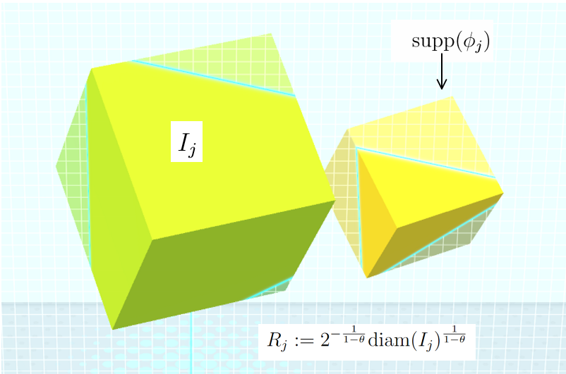
In Figure 1 we compare the size of IjI_{j} with the size of the support of ϕj.\phi_{j}.

Refer to caption
Figure 1. Let j∈ℕj\in\mathbb{N}. The replacement b~j\tilde{b}_{j} of bjb_{j} is defined by modifying its support. To do so, we make the convolution between bjb_{j} with the L1L^{1}-normalised function ϕj\phi_{j} whose support is proportional to Rj.R_{j}.

Now, going back to the analysis of (3.7), note that

|{x∈G∖I∗:|T​b​(x)|>α2}|\displaystyle|\{x\in G\setminus I^{*}:|Tb(x)|>\frac{\alpha}{2}\}|
≤|{x∈G∖I∗:|T​b​(x)−T​b~​(x)|>α4}|+|{x∈G∖I∗:|T​b~​(x)|>α4}|\displaystyle\leq|\{x\in G\setminus I^{*}:|Tb(x)-T\tilde{b}(x)|>\frac{\alpha}{4}\}|+|\{x\in G\setminus I^{*}:|T\tilde{b}(x)|>\frac{\alpha}{4}\}|
≤4α​‖T⁡(b−b~)‖L1​(G∖I∗)+|{x∈G∖I∗:|T​b~​(x)|>α4}|,\displaystyle\leq\frac{4}{\alpha}\|T(b-\tilde{b})\|_{L^{1}(G\setminus I^{*})}+|\{x\in G\setminus I^{*}:|T\tilde{b}(x)|>\frac{\alpha}{4}\}|,

and let us take into account the estimate:

‖T⁡(b−b~)‖L1​(G∖I∗)\displaystyle\|T(b-\tilde{b})\|_{L^{1}(G\setminus I^{*})} =∫G∖I∗|T​b​(x)−T​b~​(x)|​𝑑x\displaystyle=\smallint\limits_{G\setminus I^{*}}|Tb(x)-T\tilde{b}(x)|dx
≤∑j∫G∖I∗|T​bj​(x)−T​b~j​(x)|​𝑑x.\displaystyle\leq\sum_{j}\smallint\limits_{G\setminus I^{*}}|Tb_{j}(x)-T\tilde{b}_{j}(x)|dx.

We are going to prove that T​b~T\tilde{b} and T​b~jT\tilde{b}_{j} are good replacements for T​bT{b} and T​bj,T{b}_{j}, respectively, on the set G∖I∗.G\setminus I^{*}. Observe that

∫G∖I∗|T​bj​(x)−T​b~j​(x)|𝑑x=∫G∖I∗|bj∗K⁡(x)−b~j∗K⁡(x)|​𝑑x\displaystyle\smallint\limits_{G\setminus I^{*}}|Tb_{j}(x)-T\tilde{b}_{j}(x)|dx=\smallint\limits_{G\setminus I^{*}}|b_{j}\ast K(x)-\tilde{b}_{j}\ast K(x)|dx
=∫G∖I∗|bj∗K⁡(x)−[bj∗ϕj∗K]​(x)|​𝑑x\displaystyle=\smallint\limits_{G\setminus I^{*}}|b_{j}\ast K(x)-[{b}_{j}\ast\phi_{j}\ast K](x)|dx
=∫G∖I∗|∫IjK⁡(y−1​x)​bj​(y)​𝑑y−∫Ij(ϕj∗K)​(y−1​x)​bj​(y)​𝑑y|​𝑑x\displaystyle=\smallint\limits_{G\setminus I^{*}}\left|\smallint\limits_{I_{j}}K(y^{-1}x)b_{j}(y)dy-\smallint\limits_{I_{j}}(\phi_{j}\ast K)(y^{-1}x){b}_{j}(y)dy\right|dx
≤∫Ij∫G∖I∗|K⁡(y−1​x)−ϕj∗K⁡(y−1​x)​|𝑑x|​bj​(y)|​𝑑y\displaystyle\leq\smallint\limits_{I_{j}}\smallint\limits_{G\setminus I^{*}}|K(y^{-1}x)-\phi_{j}\ast K(y^{-1}x)|dx|b_{j}(y)|dy
≤∫Ij∫|z|>diam​(Ij)|K⁡(z)−ϕj∗K⁡(z)​|𝑑z|​bj​(y)|​𝑑y\displaystyle\leq\smallint\limits_{I_{j}}\smallint\limits_{|z|>\textnormal{diam}(I_{j})}|K(z)-\phi_{j}\ast K(z)|dz|b_{j}(y)|dy
≤∫Ij∫|z|>diam​(Ij)|K⁡(z)−ϕj∗K⁡(z)​|𝑑z|​bj​(y)|​𝑑y,\displaystyle\leq\smallint\limits_{I_{j}}\smallint\limits_{|z|>\textnormal{diam}(I_{j})}|K(z)-\phi_{j}\ast K(z)|dz|b_{j}(y)|dy,

where, in the last line we have used the changes of variables x↦z=y−1​x,x\mapsto z=y^{-1}x, and then we observe that |z|>diam​(Ij)|z|>\textnormal{diam}(I_{j}) when x∈G∖I∗x\in G\setminus I^{*} and y∈Ij.y\in I_{j}. Using that ϕj\phi_{j} is supported in a ball of radius

Rj:=2−11−θ​diam​(Ij)11−θR_{j}:=2^{-\frac{1}{1-\theta}}\textnormal{diam}(I_{j})^{\frac{1}{1-\theta}}

and that ‖ϕj‖L∞≤1/|B⁡(e,Rj)|,\|\phi_{j}\|_{L^{\infty}}\leq 1/|B(e,R_{j})|, we have that

∫|z|>diam​(Ij)|K⁡(z)−ϕj∗K⁡(z)|​𝑑z\displaystyle\smallint\limits_{|z|>\textnormal{diam}(I_{j})}|K(z)-\phi_{j}\ast K(z)|dz
=∫|z|>diam​(Ij)|K⁡(z)​∫|y|<2−11−θ​diam​(Ij)11−θϕj​(y)​𝑑y−∫|y|<2−11−θ​diam​(Ij)11−θK⁡(y−1​z)​ϕj​(y)​𝑑y|​𝑑z\displaystyle=\smallint\limits_{|z|>\textnormal{diam}(I_{j})}\left|K(z)\smallint\limits_{|y|<2^{-\frac{1}{1-\theta}}\textnormal{diam}(I_{j})^{\frac{1}{1-\theta}}}\phi_{j}(y)dy-\smallint\limits_{|y|<2^{-\frac{1}{1-\theta}}\textnormal{diam}(I_{j})^{\frac{1}{1-\theta}}}K(y^{-1}z)\phi_{j}(y)dy\right|dz
=∫|z|>diam​(Ij)|∫|y|<2−11−θ​diam​(Ij)11−θ(K⁡(z)−K⁡(y−1​z))​ϕj​(y)​𝑑y|​𝑑z\displaystyle=\smallint\limits_{|z|>\textnormal{diam}(I_{j})}\left|\,\smallint\limits_{|y|<2^{-\frac{1}{1-\theta}}\textnormal{diam}(I_{j})^{\frac{1}{1-\theta}}}(K(z)-K(y^{-1}z))\phi_{j}(y)dy\right|dz
≤∫|y|<2−11−θ​diam​(Ij)11−θ∫|z|>diam​(Ij)|K⁡(y−1​z)−K⁡(z)​|𝑑z|​ϕj​(y)|​𝑑y\displaystyle\leq\smallint\limits_{|y|<2^{-\frac{1}{1-\theta}}\textnormal{diam}(I_{j})^{\frac{1}{1-\theta}}}\smallint\limits_{|z|>\textnormal{diam}(I_{j})}|K(y^{-1}z)-K(z)|dz|\phi_{j}(y)|dy
≤1|B⁡(e,Rj)|​∫|y|<Rj∫|z|>2​Rj(1−θ)|K⁡(y−1​z)−K⁡(z)|​𝑑z​𝑑y\displaystyle\leq\frac{1}{|B(e,R_{j})|}\smallint\limits_{|y|<R_{j}}\smallint\limits_{|z|>2R_{j}^{(1-\theta)}}|K(y^{-1}z)-K(z)|dz\,dy
≲1Rjn​∫|y|<Rj∫|z|>2​Rj(1−θ)|K⁡(y−1​z)−K⁡(z)|​𝑑z​𝑑y\displaystyle\lesssim\frac{1}{R_{j}^{n}}\smallint\limits_{|y|<R_{j}}\smallint\limits_{|z|>2R_{j}^{(1-\theta)}}|K(y^{-1}z)-K(z)|dz\,dy
≤[K]H∞,θ​(G),\displaystyle\leq[K]_{H_{\infty,\theta}(G)},

where we have used that 2​Rj1−θ=diam​(Ij).2R_{j}^{1-\theta}=\textnormal{diam}(I_{j}). Now, the inequalities above allow us to finish the estimate of ‖T⁡(b−b~)‖L1​(G∖I∗).\|T(b-\tilde{b})\|_{L^{1}(G\setminus I^{*})}. Indeed,

‖T⁡(b−b~)‖L1​(G∖I∗)\displaystyle\|T(b-\tilde{b})\|_{L^{1}(G\setminus I^{*})} ≤∑j∫Ij∫G∖I∗|K⁡(y−1​x)−ϕj∗K⁡(y−1​x)​|𝑑x|​bj​(y)|​𝑑y\displaystyle\leq\sum_{j}\smallint\limits_{I_{j}}\smallint\limits_{G\setminus I^{*}}|K(y^{-1}x)-\phi_{j}\ast K(y^{-1}x)|dx|b_{j}(y)|dy
≤∑j∫Ij∫|z|>diam​(Ij)|K⁡(z)−ϕj∗K⁡(z)​|𝑑z|​bj​(y)|​𝑑y\displaystyle\leq\sum_{j}\smallint\limits_{I_{j}}\smallint\limits_{|z|>\textnormal{diam}(I_{j})}|K(z)-\phi_{j}\ast K(z)|dz|b_{j}(y)|dy
≲[K]H∞,θ​(G)​∑j∫Ij|bj​(y)|​𝑑y≤[K]H∞,θ​(G)​‖b‖L1\displaystyle\lesssim[K]_{H_{\infty,\theta}(G)}\sum_{j}\smallint\limits_{I_{j}}|b_{j}(y)|dy\leq[K]_{H_{\infty,\theta}(G)}\|b\|_{L^{1}}
≲[K]H∞,θ​(G)​‖f‖L1.\displaystyle\lesssim[K]_{H_{\infty,\theta}(G)}\|f\|_{L^{1}}.

Putting together the estimates above we deduce that

|{x∈G∖I∗:|T​b​(x)|>α2}|≤4α​‖T​b−T​b~‖L1​(G∖I∗)+|{x∈G∖I∗:|T​b~​(x)|>α4}|\displaystyle|\{x\in G\setminus I^{*}:|Tb(x)|>\frac{\alpha}{2}\}|\leq\frac{4}{\alpha}\|Tb-T\tilde{b}\|_{L^{1}(G\setminus I^{*})}+|\{x\in G\setminus I^{*}:|T\tilde{b}(x)|>\frac{\alpha}{4}\}|
≲4α​[K]H∞,θ​(G)​‖f‖L1+|{x∈G∖I∗:|T​b~​(x)|>α4}|.\displaystyle\lesssim\frac{4}{\alpha}[K]_{H_{\infty,\theta}(G)}\|f\|_{L^{1}}+|\{x\in G\setminus I^{*}:|T\tilde{b}(x)|>\frac{\alpha}{4}\}|.

Now, we will estimate the term in the right hand side of the previous inequality. Indeed, note that

|{x∈G∖I∗:|T​b~​(x)|>α4}|≤|{x∈G∖I∗:|T​b~​(x)|2>α216}||\{x\in G\setminus I^{*}:|T\tilde{b}(x)|>\frac{\alpha}{4}\}|\leq|\{x\in G\setminus I^{*}:|T\tilde{b}(x)|^{2}>\frac{\alpha^{2}}{16}\}|
≤16α2​‖T​b~‖L22.\leq\frac{16}{\alpha^{2}}\|T\tilde{b}\|_{L^{2}}^{2}.

From now, let us consider the positive operator

−Δ~=1+ℒG.-\tilde{\Delta}=1+\mathcal{L}_{G}. (3.14)

Now, using (1.2) we deduce that T​(−Δ~)n​θ4T(-\tilde{\Delta})^{\frac{n\theta}{4}} is bounded on L2,L^{2}, (see Remark 2.2) and then

‖T​b~‖L22≤‖T​(−Δ~)n​θ4‖ℬ⁡(L2)2​‖(−Δ~)−n​θ4​b~‖L22.\|T\tilde{b}\|^{2}_{L^{2}}\leq\|T(-\tilde{\Delta})^{\frac{n\theta}{4}}\|_{\mathscr{B}(L^{2})}^{2}\|(-\tilde{\Delta})^{-\frac{n\theta}{4}}\tilde{b}\|_{L^{2}}^{2}.

In order to estimate the L2L^{2}-norm, let us use the following lemma whose proof we postpone for a moment.

Lemma 3.1.

The function F:=(−Δ~)−n​θ4​b~F:=(-\tilde{\Delta})^{-\frac{n\theta}{4}}\tilde{b} can be decomposed as the sums F=F1+F2,F=F_{1}+F_{2}, where ‖F2‖L22≤C​α​γ​‖f‖L1,\|F_{2}\|_{L^{2}}^{2}\leq C\alpha\gamma\|f\|_{L^{1}}, and F1F_{1} is also a sum of functions F1jF_{1}^{j} with the following property.

  • •

    There exists M0∈ℕ,M_{0}\in\mathbb{N}, and A′>0,A^{\prime}>0, such that F1=∑j:diam​(Ij)<1F1jF_{1}=\sum_{j:\textnormal{diam}(I_{j})<1}F_{1}^{j}, ‖F1j‖L22≤A′​α2​|Ij|,\|F_{1}^{j}\|_{L^{2}}^{2}\leq A^{\prime}\alpha^{2}|I_{j}|, and for any x∈ℝn,x\in\mathbb{R}^{n}, there at most M0M_{0} values of jj such that F1j​(x)≠0.F_{1}^{j}(x)\neq 0.

Let us continue with the proof of Theorem 1.1. Using Lemma 3.1 and the inequalities in (3.5) we have that

‖T​b~‖L22\displaystyle\|T\tilde{b}\|_{L^{2}}^{2} ≲‖F1‖L22+‖F2‖L22≲α​γ​‖f‖L1+∑j‖F1j‖L22\displaystyle\lesssim\|F_{1}\|_{L^{2}}^{2}+\|F_{2}\|_{L^{2}}^{2}\lesssim\alpha\gamma\|f\|_{L^{1}}+\sum_{j}\|F_{1}^{j}\|_{L^{2}}^{2}
≲α​γ​‖f‖L1+∑jα2​|Ij|≲α​γ​‖f‖L1+α2​(γ​α)−1​‖f‖L1\displaystyle\lesssim\alpha\gamma\|f\|_{L^{1}}+\sum_{j}\alpha^{2}|I_{j}|\lesssim\alpha\gamma\|f\|_{L^{1}}+\alpha^{2}(\gamma\alpha)^{-1}\|f\|_{L^{1}}
=(γ−1+γ)​α​‖f‖L1.\displaystyle=(\gamma^{-1}+\gamma)\alpha\|f\|_{L^{1}}.

Consequently

|{x∈G∖I∗:|T​b~​(x)|>α4}|≲16α2​‖T​b~‖L22≲(γ−1+γ)​α−1​‖f‖L1.|\{x\in G\setminus I^{*}:|T\tilde{b}(x)|>\frac{\alpha}{4}\}|\lesssim\frac{16}{\alpha^{2}}\|T\tilde{b}\|_{L^{2}}^{2}\lesssim(\gamma^{-1}+\gamma)\alpha^{-1}\|f\|_{L^{1}}.

Thus, we have proved that

|{x∈ℝn:|T​f​(x)|>α}|≤Cγ,[K]H∞,θ​(G)​α−1​‖f‖L1,|\{x\in\mathbb{R}^{n}:|Tf(x)|>\alpha\}|\leq C_{\gamma,[K]_{H_{\infty,\theta}(G)}}\alpha^{-1}\|f\|_{L^{1}}, (3.15)

with C:=Cγ,[K]H∞,θ​(G)C:=C_{\gamma,[K]_{H_{\infty,\theta}(G)}} independent of f.f. Because γ\gamma is fixed we have proved the weak (1,1)(1,1) type of T.T. Note that the LpL^{p}-boundedness of TT can be deduced from Marcinkiewicz interpolation theorem and the standard duality argument. Thus, the proof is complete once we proved the statement in Lemma 3.1. To do so, let us consider the right-convolution kernel kθ:=(−Δ~)−n​θ4​δk_{\theta}:=(-\tilde{\Delta})^{-\frac{n\theta}{4}}\delta of the operator (−Δ~)−n​θ4(-\tilde{\Delta})^{-\frac{n\theta}{4}} and let us split the function (−Δ~)−n​θ4​b~​(x)(-\tilde{\Delta})^{-\frac{n\theta}{4}}\tilde{b}(x) as follows:

(−Δ~)−n​θ4​b~​(x)\displaystyle(-\tilde{\Delta})^{-\frac{n\theta}{4}}\tilde{b}(x) =∑j(−Δ~)−n​θ4​b~j​(x)=∑jb~j∗kθ​(x)\displaystyle=\sum_{j}(-\tilde{\Delta})^{-\frac{n\theta}{4}}\tilde{b}_{j}(x)=\sum_{j}\tilde{b}_{j}\ast k_{\theta}(x)
=∑j:x∈Ijb~j∗kθ(x)+∑j:x≁Ijb~j∗kθ(x)=:G1(x)+G2(x),\displaystyle=\sum_{j:x\in I_{j}}\tilde{b}_{j}\ast k_{\theta}(x)+\sum_{j:x\nsim I_{j}}\tilde{b}_{j}\ast k_{\theta}(x)=:G_{1}(x)+G_{2}(x),

where G1(x):=∑j:x∼Ijb~j∗kθ(x)G_{1}(x):=\sum_{j:x\sim I_{j}}\tilde{b}_{j}\ast k_{\theta}(x) and G2(x):=∑j:x≁Ijb~j∗kθ(x).G_{2}(x):=\sum_{j:x\nsim I_{j}}\tilde{b}_{j}\ast k_{\theta}(x). We have denoted by x∼Ij,x\sim I_{j}, if xx belongs to IjI_{j} or to some Ij′I_{j^{\prime}} with non-empty intersection with Ij.I_{j}. By the properties of these sets there are at most M0M_{0} sets Ij′I_{j^{\prime}} such that Ij∩Ij′≠∅.I_{j}\cap I_{j^{\prime}}\neq\emptyset. Also, the notation x≁Ijx\nsim I_{j} will be employed to define the opposite of the previous property.

Let us prove the estimate

‖G2‖L22≤C​α​γ​‖f‖L1.\|G_{2}\|_{L^{2}}^{2}\leq C\alpha\gamma\|f\|_{L^{1}}. (3.16)

Observe that

‖G2‖L1\displaystyle\|G_{2}\|_{L^{1}} =∫G|∑j:x≁Ijbj∗ϕj∗kθ(x)|dx≤∑j:x≁Ij∫G|bj∗ϕj∗kθ(x)|dx\displaystyle=\smallint\limits_{G}|\sum_{j:x\nsim I_{j}}{b}_{j}\ast\phi_{j}\ast k_{\theta}(x)|dx\leq\sum_{j:x\nsim I_{j}}\smallint\limits_{G}|{b}_{j}\ast\phi_{j}\ast k_{\theta}(x)|dx
≤∑j‖bj∗ϕj∗kθ‖L1≤∑j‖bj‖L1​‖ϕj∗kθ‖L1.\displaystyle\leq\sum_{j}\|{b}_{j}\ast\phi_{j}\ast k_{\theta}\|_{L^{1}}\leq\sum_{j}\|{b}_{j}\|_{L^{1}}\|\phi_{j}\ast k_{\theta}\|_{L^{1}}.

Note that (−Δ~)−n​θ4(-\tilde{\Delta})^{-\frac{n\theta}{4}} is a pseudo-differential operator of order −nθ/2,-n\theta/2, and consequently, its kernel satisfies the estimate

|kθ​(x)|≤C​|x|−(−n​θ2+n)≲|x|−n⁡(1−θ2),x∈G∖{e}.|k_{\theta}(x)|\leq C|x|^{{-(-\frac{n\theta}{2}+n)}}\lesssim|x|^{-{n(1-\frac{\theta}{2})}},\,x\in G\setminus\{e\}.

The condition 0<θ<1,0<\theta<1, implies that kθk_{\theta} is an integrable distribution and then

‖ϕj∗kθ‖L1≲‖ϕj‖L1​‖kθ‖L1=‖kθ‖L1<∞.\|\phi_{j}\ast k_{\theta}\|_{L^{1}}\lesssim\|\phi_{j}\|_{L^{1}}\|k_{\theta}\|_{L^{1}}=\|k_{\theta}\|_{L^{1}}<\infty.

So, we have that

‖G2‖L1≲∑j‖bj‖L1≲‖f‖L1.\displaystyle\|G_{2}\|_{L^{1}}\lesssim\sum_{j}\|b_{j}\|_{L^{1}}\lesssim\|f\|_{L^{1}}.

So, for the proof of (3.16), and in view of the inequality ‖G2‖L22≤‖G2‖L1​‖G2‖L∞\|G_{2}\|^{2}_{L^{2}}\leq\|G_{2}\|_{L^{1}}\|G_{2}\|_{L^{\infty}} is enough to show that ‖G2‖L∞≲α​γ​‖f‖L1.\|G_{2}\|_{L^{\infty}}\lesssim\alpha\gamma\|f\|_{L^{1}}. To do this, let us consider jj such that x≁Ij.x\nsim I_{j}. Since b~j∗kθ=bj∗ϕj∗kθ,\tilde{b}_{j}\ast k_{\theta}={b}_{j}\ast\phi_{j}\ast k_{\theta}, one has that

|bj∗ϕj∗kθ​(x)|\displaystyle|{b}_{j}\ast\phi_{j}\ast k_{\theta}(x)| ≤∫Ij|ϕj∗kθ​(y−1​x)|​|bj​(y)|​𝑑y≤supy∈Ij|ϕj∗kθ​(y−1​x)|​∫Ij|bj​(y)|​𝑑y\displaystyle\leq\smallint\limits_{I_{j}}|\phi_{j}\ast k_{\theta}(y^{-1}x)||b_{j}(y)|dy\leq\sup_{y\in I_{j}}|\phi_{j}\ast k_{\theta}(y^{-1}x)|\smallint\limits_{I_{j}}|b_{j}(y)|dy
=supy∈Ij|ϕj∗kθ(y−1x)||Ij|×1|Ij|∫Ij|bj(y)|dy.\displaystyle=\sup_{y\in I_{j}}|\phi_{j}\ast k_{\theta}(y^{-1}x)||I_{j}|\times\frac{1}{|I_{j}|}\smallint\limits_{I_{j}}|b_{j}(y)|dy.

To continue, we follow as in [24, Page 26] the observation of Fefferman, that in view of the property x≁Ij,x\nsim I_{j}, we have that ϕj∗kθ​(y−1​x)\phi_{j}\ast k_{\theta}(y^{-1}x) is essentially constant over the ball Ij=B⁡(xj,rj)I_{j}=B(x_{j},r_{j}) and we can estimate

supy∈Ij|ϕj∗kθ​(y−1​x)|​|Ij|≲∫Ij|ϕj∗kθ​(y′−1​x)|​d​y′.\sup_{y\in I_{j}}|\phi_{j}\ast k_{\theta}(y^{-1}x)||I_{j}|\lesssim\smallint\limits_{I_{j}}|\phi_{j}\ast k_{\theta}(y^{\prime-1}x)|dy^{\prime}. (3.17)

On the other hand, observe that the positivity of the kernel kθ,k_{\theta}, and of ϕj\phi_{j} leads to

∫Ij|ϕj∗kθ​(y′−1​x)|​d​y′​1|Ij|​∫Ij|bj​(y)|​𝑑y\displaystyle\smallint\limits_{I_{j}}|\phi_{j}\ast k_{\theta}(y^{\prime-1}x)|dy^{\prime}\frac{1}{|I_{j}|}\smallint\limits_{I_{j}}|b_{j}(y)|dy =∫G|ϕj∗kθ​(y′−1​x)|​(1|Ij|​∫Ij|bj​(y)|​𝑑y)​1Ij​(y′)​d​y′\displaystyle=\smallint\limits_{G}|\phi_{j}\ast k_{\theta}(y^{\prime-1}x)|\left(\frac{1}{|I_{j}|}\smallint\limits_{I_{j}}|b_{j}(y)|dy\right)1_{I_{j}}(y^{\prime})dy^{\prime}
=(1|Ij|​∫Ij|bj​(y)|​𝑑y×1Ij)∗ϕj∗kθ​(x).\displaystyle=\left(\frac{1}{|I_{j}|}\smallint\limits_{I_{j}}|b_{j}(y)|dy\times 1_{I_{j}}\right)\ast\phi_{j}\ast k_{\theta}(x).

Consequently, we have

|G2​(x)|\displaystyle|G_{2}(x)| ≤∑j:x≁Ij|b~j∗kθ(x)|≲∑j:x≁Ij(1|Ij|∫Ij|bj(y)|dy×1Ij)∗ϕj∗kθ(x)\displaystyle\leq\sum_{j:x\nsim I_{j}}|\tilde{b}_{j}\ast k_{\theta}(x)|\lesssim\sum_{j:x\nsim I_{j}}\left(\frac{1}{|I_{j}|}\smallint\limits_{I_{j}}|b_{j}(y)|dy\times 1_{I_{j}}\right)\ast\phi_{j}\ast k_{\theta}(x)
≲∑j:x≁Ijγα×1Ij∗ϕj∗kθ(x)=∫G∑j:x≁Ijγα×1Ij∗ϕj(z)kθ(z−1x)dz\displaystyle\lesssim\sum_{j:x\nsim I_{j}}\gamma\alpha\times 1_{I_{j}}\ast\phi_{j}\ast k_{\theta}(x)=\smallint\limits_{G}\sum_{j:x\nsim I_{j}}\gamma\alpha\times 1_{I_{j}}\ast\phi_{j}(z)k_{\theta}(z^{-1}x)dz
≲γα∥kθ∥L1‖∑j:x≁Ij1Ij∗ϕj‖L∞.\displaystyle\lesssim\gamma\alpha\|k_{\theta}\|_{L^{1}}\left\|\sum_{j:x\nsim I_{j}}1_{I_{j}}\ast\phi_{j}\right\|_{L^{\infty}}.

By observing that the supports of the functions 1Ij∗ϕj1_{I_{j}}\ast\phi_{j}’s have bounded overlaps we have that ‖∑j:x≁Ij1Ij∗ϕj‖L∞<∞,\left\|\sum_{j:x\nsim I_{j}}1_{I_{j}}\ast\phi_{j}\right\|_{L^{\infty}}<\infty, and that ‖G2‖L∞≲γ​α.\|G_{2}\|_{L^{\infty}}\lesssim\gamma\alpha.

It remains only to prove that ‖G1‖L22≲α​‖f‖L1.\|G_{1}\|_{L^{2}}^{2}\lesssim\alpha\|f\|_{L^{1}}. Let us define

Gj​(x):={bj∗ϕj∗kθ​(x), x∈Ij,0,otherwise. G^{j}(x):=\begin{cases}{b}_{j}\ast\phi_{j}\ast k_{\theta}(x),&\text{ }x\in I_{j},\\ 0,&\,\text{otherwise. }\end{cases} (3.18)

Then G1=∑jGjG_{1}=\sum_{j}G^{j} and in view of the finite overlapping of the balls IjI_{j}’s, there is M0∈ℕ,M_{0}\in\mathbb{N}, such that for any x∈G,x\in G, Gj​(x)≠0,G^{j}(x)\neq 0, for at most M0M_{0} values of j.j. Therefore, we have that

∫G|G1​(x)|2​𝑑x\displaystyle\smallint_{G}|G_{1}(x)|^{2}dx ≤M0​∑j∫G|Gj​(x)|2​𝑑x=∑j∫Ij|bj∗ϕj∗kθ​(x)|2​𝑑x\displaystyle\leq M_{0}\sum_{j}\smallint_{G}|G^{j}(x)|^{2}dx=\sum_{j}\smallint_{I_{j}}|{b}_{j}\ast\phi_{j}\ast k_{\theta}(x)|^{2}dx
≤∑j‖bj‖L12​‖ϕj∗kθ‖L22≤∑jα2​γ2​|Ij|2​‖ϕj∗kθ‖L22.\displaystyle\leq\sum_{j}\|{b}_{j}\|_{L^{1}}^{2}\|\phi_{j}\ast k_{\theta}\|_{L^{2}}^{2}\leq\sum_{j}\alpha^{2}\gamma^{2}|I_{j}|^{2}\|\phi_{j}\ast k_{\theta}\|_{L^{2}}^{2}.

Because our argument is purely local let us use the diffeomorphism ω=exp:ν→ν′\omega=\textnormal{exp}:\nu\rightarrow\nu^{\prime} in (3.8). Because B⁡(e,c)⊂ν′,{B}(e,c)\subset\nu^{\prime}, we can estimate the norm ‖ϕj∗kθ‖L2\|\phi_{j}\ast k_{\theta}\|_{L^{2}} in a small neighbourhood ν′\nu^{\prime} of the identity element e∈G.e\in G. Note that for any jj with diam​(Ij)<c,\textnormal{diam}(I_{j})<c, we have the inclusion B⁡(e,Rj)⊂ν′.B(e,R_{j})\subset\nu^{\prime}. So, we have

∥ϕj∗kθ∥L22=∥(1+ℒG)−n​θ4ϕj∥L22=∥ϕj∥H−nθ/2≍∥(1+ℒℝn)−n​θ4ϕj′∥L22,\|\phi_{j}\ast k_{\theta}\|_{L^{2}}^{2}=\|(1+\mathcal{L}_{G})^{-\frac{n\theta}{4}}\phi_{j}\|^{2}_{L^{2}}=\|\phi_{j}\|_{H^{-n\theta/2}}\asymp\|(1+\mathcal{L}_{\mathbb{R}^{n}})^{-\frac{n\theta}{4}}{\phi}^{\prime}_{j}\|_{L^{2}}^{2},

where

ϕj′=ϕj∘ω=1B⁡(e,Rj)​1B⁡(e,Rj)∘ω,supp​(ϕj′)⊂ν.\phi_{j}^{\prime}=\phi_{j}\circ\omega=\frac{1}{B(e,R_{j})}1_{B(e,R_{j})}\circ\omega,\,\,\textnormal{supp}(\phi_{j}^{\prime})\subset\nu.

Note that (1+ℒℝn)−n​θ4(1+\mathcal{L}_{\mathbb{R}^{n}})^{-\frac{n\theta}{4}} is bounded on L2,L^{2}, and clearly ϕj′∈L2,\phi_{j}^{\prime}\in L^{2}, so that ϕj′∈Dom​((1+ℒℝn)−n​θ4).\phi_{j}^{\prime}\in\textnormal{Dom}((1+\mathcal{L}_{\mathbb{R}^{n}})^{-\frac{n\theta}{4}}). Also,

supp​[ϕj′]⊂B⁡(0,Rj′),Rj′∼Rj.\textnormal{supp}[\phi_{j}^{\prime}]\subset{B}(0,R_{j}^{\prime}),\,R_{j}^{\prime}\sim R_{j}. (3.19)

Define for any j,j,

ψj′​(X):=|B⁡(0,Rj′)|​ϕj′​(Rj′​X),X∈ν.\psi_{j}^{\prime}(X):=|B(0,R_{j}^{\prime})|\phi_{j}^{\prime}(R_{j}^{\prime}X),\,X\in\nu.

Then, one has the identity

ϕj′​(X)=1|B⁡(0,Rj′)|​ψj′​(XRj′),X∈ν.\phi_{j}^{\prime}(X)=\frac{1}{|B(0,R_{j}^{\prime})|}\psi_{j}^{\prime}\left(\frac{X}{R_{j}^{\prime}}\right),\,X\in\nu.

Observe that |B⁡(0,Rj′)|=vn​Rj′n,|B(0,R_{j}^{\prime})|=v_{n}{R_{j}^{\prime}}^{n}, where vnv_{n} is the volume of the unite ball B⁡(0,1).B(0,1). Also, note that ‖ψj′‖L∞=1,\|\psi_{j}^{\prime}\|_{L^{\infty}}=1, and supp​(ψj′)⊂B⁡(0,1).\textnormal{supp}(\psi_{j}^{\prime})\subset B(0,1). Using the Plancherel theorem, we have that

‖(1+ℒℝn)−n​θ4​ϕj′‖L2\displaystyle\|(1+\mathcal{L}_{\mathbb{R}^{n}})^{-\frac{n\theta}{4}}{\phi}_{j}^{\prime}\|_{L^{2}} =‖(1+|η|2)−n​θ4​ℱℝn​[ϕj′]​(η)‖L2\displaystyle=\|(1+|\eta|^{2})^{-\frac{n\theta}{4}}\mathscr{F}_{\mathbb{R}^{n}}[\phi_{j}^{\prime}](\eta)\|_{L^{2}}
=‖(1+|η|2)−n​θ4​ℱℝn​[1|B⁡(0,Rj′)|​ψj′​(⋅Rj′)]​(η)‖L2\displaystyle=\|(1+|\eta|^{2})^{-\frac{n\theta}{4}}\mathscr{F}_{\mathbb{R}^{n}}\left[\frac{1}{|B(0,R_{j}^{\prime})|}\psi_{j}^{\prime}\left(\frac{\cdot}{R_{j}^{\prime}}\right)\right]\left(\eta\right)\|_{L^{2}}
=(1/vn)​‖(1+|η|2)−n​θ4​ℱℝn​[1Rj′n​ψj′​(⋅Rj′)]​(η)‖L2\displaystyle=(1/v_{n})\|(1+|\eta|^{2})^{-\frac{n\theta}{4}}\mathscr{F}_{\mathbb{R}^{n}}\left[\frac{1}{{R_{j}^{\prime}}^{n}}\psi_{j}^{\prime}\left(\frac{\cdot}{R_{j}^{\prime}}\right)\right]\left(\eta\right)\|_{L^{2}}
=(1/vn)​‖(1+|η|2)−n​θ4​ℱℝn​[ψj′]​(Rj′​η)‖L2.\displaystyle=(1/v_{n})\|(1+|\eta|^{2})^{-\frac{n\theta}{4}}\mathscr{F}_{\mathbb{R}^{n}}[\psi_{j}^{\prime}]\left(R_{j}^{\prime}\eta\right)\|_{L^{2}}.

Observe that

‖(1+|η|2)−n​θ4​ℱℝn​[ψj′]​(Rj​η)‖L22\displaystyle\|(1+|\eta|^{2})^{-\frac{n\theta}{4}}\mathscr{F}_{\mathbb{R}^{n}}[\psi_{j}^{\prime}]\left(R_{j}\eta\right)\|_{L^{2}}^{2} =∫|(1+|η|2)−n​θ4​ℱℝn​[ψj′]​(Rj​η)|2​𝑑η\displaystyle=\smallint\limits|(1+|\eta|^{2})^{-\frac{n\theta}{4}}\mathscr{F}_{\mathbb{R}^{n}}[\psi_{j}^{\prime}]\left(R_{j}\eta\right)|^{2}d\eta
=Rj′−n​∫|(1+|Rj′−1​z|2)−n​θ4​ℱℝn​[ψj′]​(z)|2​𝑑z\displaystyle={R^{\prime}_{j}}^{-n}\smallint\limits|(1+|{R^{\prime}_{j}}^{-1}z|^{2})^{-\frac{n\theta}{4}}\mathscr{F}_{\mathbb{R}^{n}}[\psi_{j}^{\prime}](z)|^{2}dz
=Rj′−n​Rj′n​θ​∫|(Rj′+|z|2)−n​θ4​ℱℝn​[ψj′]​(z)|2​𝑑z\displaystyle={R^{\prime}_{j}}^{-n}{R^{\prime}_{j}}^{n\theta}\smallint\limits|(R_{j}^{\prime}+|z|^{2})^{-\frac{n\theta}{4}}\mathscr{F}_{\mathbb{R}^{n}}[\psi_{j}^{\prime}](z)|^{2}dz
≤Rj′−n​Rj′n​θ​∫|(|z|2)−n​θ4​ℱℝn​[ψj′]​(z)|2​𝑑z\displaystyle\leq{R^{\prime}_{j}}^{-n}{R^{\prime}_{j}}^{n\theta}\smallint\limits|(|z|^{2})^{-\frac{n\theta}{4}}\mathscr{F}_{\mathbb{R}^{n}}[\psi_{j}^{\prime}](z)|^{2}dz
≍Rj′−n​Rj′n​θ​∫|(−Δ)−n​θ4​ψj′​(x)|2​𝑑x\displaystyle\asymp{R^{\prime}_{j}}^{-n}{R^{\prime}_{j}}^{n\theta}\smallint\limits|(-\Delta)^{-\frac{n\theta}{4}}\psi_{j}^{\prime}(x)|^{2}dx
=Rj−n⁡(1−θ)​‖(−Δ)−n​θ4​ψj′‖L22.\displaystyle=R_{j}^{-n(1-\theta)}\|(-\Delta)^{-\frac{n\theta}{4}}\psi_{j}^{\prime}\|_{L^{2}}^{2}.

By the compactness of G,G, for all ε>0,\varepsilon>0, there exists a finite number of elements x0ε=eG,xkε,x_{0}^{\varepsilon}=e_{G},x_{k}^{\varepsilon}, 1⩽k⩽N0​(ε),1\leqslant k\leqslant N_{0}(\varepsilon), in G,G, and some smooth functions χkε∈C∞​(G,[0,1]),\chi_{k}^{\varepsilon}\in C^{\infty}(G,[0,1]), supported in B⁡(eG,ε2),B(e_{G},\frac{\varepsilon}{2}), such that

G=⋃k=1N0​(ε)B⁡(xkε,ε/4), and ​∑j=0N0​(ε)χkε​(xk−1​x)=1,x∈G.G=\bigcup_{k=1}^{N_{0}(\varepsilon)}B(x_{k}^{\varepsilon},\varepsilon/4),\,\,\,\textnormal{ and }\sum_{j=0}^{N_{0}(\varepsilon)}\chi_{k}^{\varepsilon}(x_{k}^{-1}x)=1,\,\,\,x\in G. (3.20)

Note that for ε>0\varepsilon>0 small enough, the support of any x↦χkε​(xk−1​x)x\mapsto\chi_{k}^{\varepsilon}(x_{k}^{-1}x) is inside of ν′.\nu^{\prime}. In consequence, we can estimate

‖(−Δ)−n​θ4​ψj′‖L2\displaystyle\|(-\Delta)^{-\frac{n\theta}{4}}\psi_{j}^{\prime}\|_{L^{2}} ≍∥(−ℒG)−n​θ4ψj′∘exp∥L2≤∑j=0N0​(ε)∥(−ℒG)−n​θ4[ψj′∘exp⋅χkε(xk−1⋅)]∥L2\displaystyle\asymp\|(-\mathcal{L}_{G})^{-\frac{n\theta}{4}}\psi_{j}^{\prime}\circ\textnormal{exp}\|_{L^{2}}\leq\sum_{j=0}^{N_{0}(\varepsilon)}\|(-\mathcal{L}_{G})^{-\frac{n\theta}{4}}[\psi_{j}^{\prime}\circ\textnormal{exp}\cdot\chi_{k}^{\varepsilon}(x_{k}^{-1}\cdot)]\|_{L^{2}}
≲∑j=0N0​(ε)∥ψj′∘exp⋅χkε(xk−1⋅)∥L2≍∥ψj′∘exp∥L2≍∥ψj′∥L2,\displaystyle\lesssim\sum_{j=0}^{N_{0}(\varepsilon)}\|\psi_{j}^{\prime}\circ\textnormal{exp}\cdot\chi_{k}^{\varepsilon}(x_{k}^{-1}\cdot)\|_{L^{2}}\asymp\|\psi_{j}^{\prime}\circ\textnormal{exp}\|_{L^{2}}\asymp\|\psi_{j}^{\prime}\|_{L^{2}},

where we have used the L2L^{2}-boundedness of the operator (−ℒG)−n​θ4(-\mathcal{L}_{G})^{-\frac{n\theta}{4}} in view of the Stein identity (see [43, Page 58])

(−ℒG)−n​θ4=(−ℒG+ProjKer​(−ℒG))−n​θ4−ProjKer​(−ℒG),(-\mathcal{L}_{G})^{-\frac{n\theta}{4}}=\left(-\mathcal{L}_{G}+\textnormal{Proj}_{\textnormal{Ker}(-\mathcal{L}_{G})}\right)^{-\frac{n\theta}{4}}-\textnormal{Proj}_{\textnormal{Ker}(-\mathcal{L}_{G})},

and of Remark 2.4 of [40]. Indeed, we have that (−ℒG)−n​θ4(-\mathcal{L}_{G})^{-\frac{n\theta}{4}} is a pseudo-differential operator on GG of order −nθ/2-n\theta/2 and hence bounded on L2​(G).L^{2}(G). Note that, this argument does not apply in the case of ℝn\mathbb{R}^{n} because the spectrum of the Euclidean Laplacian is continuous and the negative powers of −Δℝn-\Delta_{\mathbb{R}^{n}} are not pseudo-differential operators while the powers of 1−Δℝn1-\Delta_{\mathbb{R}^{n}} are pseudo-differential operators with symbols in the Kohn-Nirenberg classes, see e.g. Taylor [45].

Continuing with the proof, since ‖ψj‖L∞=1\|\psi_{j}\|_{L^{\infty}}=1 and ψj\psi_{j} is supported in the unit ball, we have that ‖ψj‖L2≤1.\|\psi_{j}\|_{L^{2}}\leq 1. Consequently,

‖ϕj∗kθ‖L22≲Rj−n⁡(1−θ)∼|Ij|−1.\|\phi_{j}\ast k_{\theta}\|_{L^{2}}^{2}\lesssim R_{j}^{-n(1-\theta)}\sim|I_{j}|^{-1}.

Finally, we deduce that

∫G|G1​(x)|2​𝑑x\displaystyle\smallint_{G}|G_{1}(x)|^{2}dx ≤∑jα2​γ2​|Ij|2​‖ϕj∗kθ‖L22≲∑jα2​γ2​|Ij|2​|Ij|−1=α2​γ2​∑j|Ij|\displaystyle\leq\sum_{j}\alpha^{2}\gamma^{2}|I_{j}|^{2}\|\phi_{j}\ast k_{\theta}\|_{L^{2}}^{2}\lesssim\sum_{j}\alpha^{2}\gamma^{2}|I_{j}|^{2}|I_{j}|^{-1}=\alpha^{2}\gamma^{2}\sum_{j}|I_{j}|
≲αγ∥f∥L1≲γα∥f∥L1,\displaystyle\lesssim\alpha\gamma\|f\|_{L^{1}}\lesssim_{\gamma}\alpha\|f\|_{L^{1}},

in view of (3.5). Consequently, we can take F2:=G2,F_{2}:=G_{2}, F1:=G1F_{1}:=G_{1} and F1j:=G1j.F_{1}^{j}:=G_{1}^{j}. Thus, the proof of Lemma 3.1 is complete as well as the proof of Theorem 1.1. ∎

4. Examples

In this section we give some applications of Theorem 1.1 on the torus, on SU​(2)≅𝕊3\textnormal{SU}(2)\cong\mathbb{S}^{3} and for oscillating multipliers. We refer the reader to [13, Section 4] for a variety of examples on the boundedness of oscillating singular integrals on Lie groups of polynomial growth.

4.1. Oscillating integrals on the torus 𝕋n\mathbb{T}^{n}

Let G=𝕋n≡ℝn/ℤn,G=\mathbb{T}^{n}\equiv\mathbb{R}^{n}/\mathbb{Z}^{n}, be the nn-torus. In this case we have the identification 𝕋^n={eℓ}ℓ∈ℤn∼ℤn\widehat{\mathbb{T}}^{n}=\{e_{\ell}\}_{\ell\in\mathbb{Z}^{n}}\sim\mathbb{Z}^{n} for its unitary dual. We have denoted eℓe_{\ell} to the exponential function eℓ​(x)=ei​2​π​ℓ⋅x,e_{\ell}(x)=e^{i2\pi\ell\cdot x}, x=(x1,⋯,xn)∈𝕋n.x=(x_{1},\cdots,x_{n})\in\mathbb{T}^{n}.

In terms of the Fourier transform of a distribution KK on the torus

K^​(ℓ):=∫𝕋ne−ℓ​(x)​K​(x)​𝑑x,ℓ∈ℤn,\widehat{K}(\ell):=\smallint_{\mathbb{T}^{n}}e_{-\ell}(x)K(x)dx,\,\,\ell\in\mathbb{Z}^{n}, (4.1)

the Fourier transform condition (1.11) becomes equivalent to the estimate

∀ℓ∈ℤn,|K^​(ℓ)|≤C​⟨ℓ⟩−n​θ2,⟨ℓ⟩:=(1+4​π2​|ℓ|2)12∼|ℓ|:=ℓ12+⋯+ℓn2.\forall\ell\in\mathbb{Z}^{n},\,\,|\widehat{K}(\ell)|\leq C\langle\ell\rangle^{-\frac{n\theta}{2}},\,\ \langle\ell\rangle:=(1+4\pi^{2}|\ell|^{2})^{\frac{1}{2}}\sim|\ell|:=\sqrt{\ell_{1}^{2}+\cdots+\ell_{n}^{2}}. (4.2)

Note that the kernel condition (1.12) takes the form

[K]H∞,θ=supR>0sup|y|<R∫|x|≥2​R1−θ|K⁡(x−y)−K⁡(x)|​𝑑x​𝑑y<∞.[K]_{H_{\infty,\theta}}=\sup_{R>0}\sup_{|y|<R}\smallint\limits_{|x|\geq 2R^{1-\theta}}|K(x-y)-K(x)|dxdy<\infty. (4.3)

In view of Theorem 1.1, a convolution operator TT associated to a convolution kernel K,K, satisfying the Fourier transform condition (4.2) and the smoothness condition (4.3) is of weak (1,1) type, that is T:L1​(𝕋n)→L1,∞​(𝕋n)T:L^{1}(\mathbb{T}^{n})\rightarrow L^{1,\infty}(\mathbb{T}^{n}) is bounded. As the referee of this manuscript pointed out, in the case of the torus 𝕋n\mathbb{T}^{n} this continity result should also be just a special case of the known result due to Fefferman [24] on ℝn\mathbb{R}^{n} for a distributions KK with its support small enough as a consequence of a periodisation argument (see e.g. [39, Chapters III and IV]).

4.2. Oscillating integrals on SU​(2)≅𝕊3\textnormal{SU}(2)\cong\mathbb{S}^{3}

Let us consider the compact Lie group of complex unitary 2×22\times 2-matrices

SU​(2)={X=[Xi​j]i,j=12∈ℂ2×2:X∗=X−1},X∗:=X¯t=[Xj​i¯]i,j=12.\textnormal{SU}(2)=\{X=[X_{ij}]_{i,j=1}^{2}\in\mathbb{C}^{2\times 2}:X^{*}=X^{-1}\},\,X^{*}:=\overline{X}^{t}=[\overline{X_{ji}}]_{i,j=1}^{2}.

Let us consider the left-invariant first-order differential operators

∂+,∂−,∂0:C∞​(SU​(2))→C∞​(SU​(2)),\partial_{+},\partial_{-},\partial_{0}:C^{\infty}(\textnormal{SU}(2))\rightarrow C^{\infty}(\textnormal{SU}(2)),

called creation, annihilation, and neutral operators respectively, (see Definition 11.5.10 of [39]) and let us define

X1=−i2(∂−+∂+),X2=12(∂−−∂+),X3=−i∂0,X_{1}=-\frac{i}{2}(\partial_{-}+\partial_{+}),\,X_{2}=\frac{1}{2}(\partial_{-}-\partial_{+}),\,X_{3}=-i\partial_{0},

where X3=[X1,X2].X_{3}=[X_{1},X_{2}]. The system X={X1,X2,X3}X=\{X_{1},X_{2},X_{3}\} is an orthonormal basis of the Lie algebra 𝔰​𝔲​(2)\mathfrak{su}(2) of SU​(2),\textnormal{SU}(2), and its positivie Laplacian is given by

ℒSU​(2)=−X12−X22−X32=−∂02−12[∂+∂−+∂−∂+].\mathcal{L}_{\textnormal{SU}(2)}=-X_{1}^{2}-X_{2}^{2}-X_{3}^{2}=-\partial_{0}^{2}-\frac{1}{2}[\partial_{+}\partial_{-}+\partial_{-}\partial_{+}]. (4.4)

We record that the unitary dual of SU​(2)\textnormal{SU}(2) (see [39]) can be identified as

SU^(2)≡{[tl]:2l∈ℕ,dl:=dimtl=(2l+1)}∼12ℕ.\widehat{\textnormal{SU}}(2)\equiv\{[t_{l}]:2l\in\mathbb{N},d_{l}:=\dim t_{l}=(2l+1)\}\sim\frac{1}{2}\mathbb{N}. (4.5)

There are explicit formulae for tlt_{l} as functions of Euler angles in terms of the so-called Legendre-Jacobi polynomials, see [39]. Again, by following e.g. [39], the spectrum of the positive Laplacian ℒSU​(2)\mathcal{L}_{\textnormal{SU}(2)} can be indexed by the sequence

λℓ:=ℓ⁡(ℓ+1),ℓ∈12​ℕ.\lambda_{\ell}:=\ell(\ell+1),\quad\ell\in\frac{1}{2}\mathbb{N}.

Because n=dim(SU​(2))=3,n=\dim(\textnormal{SU}(2))=3, the Fourier transform condition (1.11) takes the form

∃C>0,∀ℓ∈12​ℕ,‖K^​(ℓ)‖op≤C​(1+ℓ⁡(ℓ+1))−3​θ4∼(1+ℓ)−3​θ2,\exists C>0,\,\forall\ell\in\frac{1}{2}\mathbb{N},\quad\|\widehat{K}(\ell)\|_{\textnormal{op}}\leq C(1+\ell(\ell+1))^{-\frac{3\theta}{4}}\sim(1+\ell)^{-\frac{3\theta}{2}}, (4.6)

where K^​(ℓ)=∫SU​(2)K⁡(Z)​tℓ​(Z)∗​𝑑Z,\widehat{K}(\ell)=\smallint_{\textnormal{SU}(2)}K(Z)t_{\ell}(Z)^{*}dZ, is the Fourier transform of the group of K.K. In view of Theorem 1.1, if KK satisfies (4.6) and the kernel condition

[K]H∞,θ:=supR>0sup|Y|<R∫|X|≥2​R1−θ|K⁡(Y−1​X)−K⁡(X)|​𝑑X​𝑑Y<∞,[K]_{H_{\infty,\theta}}:=\sup_{R>0}\sup_{|Y|<R}\smallint\limits_{|X|\geq 2R^{1-\theta}}|K(Y^{-1}X)-K(X)|dXdY<\infty, (4.7)

then TT is of weak (1,1) type, that is T:L1​(SU​(2))→L1,∞​(SU​(2))T:L^{1}(\textnormal{SU}(2))\rightarrow L^{1,\infty}(\textnormal{SU}(2)) extends to a bounded operator. In (4.7), |X||X| denotes the norm of X∈SU​(2)X\in\textnormal{SU}(2) with respect to the geodesic distance on SU​(2)\textnormal{SU}(2).

4.3. Application to oscillating multipliers

Let us illustrate our main Theorem 1.1 in the context of oscillating Fourier multipliers. On G,G, the prototype of a oscillating singular integral is the spectral multiplier of ℒG,\mathcal{L}_{G}, given by

Tθ​(ℒG):=(1+ℒG)−n​θ4​ei​(1+ℒG)θ2,  0≤θ<1.T_{\theta}(\mathcal{L}_{G}):=(1+\mathcal{L}_{G})^{-\frac{n\theta}{4}}e^{i(1+\mathcal{L}_{G})^{\frac{\theta}{2}}},\,\,0\leq\theta<1. (4.8)

Indeed, Tθ​(ℒG)T_{\theta}(\mathcal{L}_{G}) is a convolution operator with right-convolution kernel K=KθK=K_{\theta} whose Fourier transform is given by

K^​(ξ)=⟨ξ⟩−n​θ2​ei​⟨ξ⟩θ,⟨ξ⟩:=(1+λ[ξ])12,[ξ]∈G^.\widehat{K}(\xi)=\langle\xi\rangle^{-\frac{n\theta}{2}}{e^{i\langle\xi\rangle^{\theta}}},\,\langle\xi\rangle:=(1+\lambda_{[\xi]})^{\frac{1}{2}},\,[\xi]\in\widehat{G}.

Let d⁡(x,y)d(x,y) be the geodesic distance on GG induced by the Riemannian metric gg. It was proved by Chen and Fan in [15] that K⁡(x)K(x) behaves essentially as cn​d​(x,e)−n​ei​cn′​d​(x,e)θ′,c_{n}d(x,e)^{-n}e^{ic_{n}^{\prime}d(x,e)^{\theta^{\prime}}}, where θ′=θθ−1,\theta^{\prime}=\frac{\theta}{\theta-1}, and consequently that

|∇K​(x)|=|(X1​K​(x),⋯,Xn​K​(x))|≲d​(x,e)−n−1+θ′,|\nabla K(x)|=|(X_{1}K(x),\cdots,X_{n}K(x))|\lesssim d(x,e)^{-n-1+\theta^{\prime}},

from which it is well known that KK satisfies (1.12), that is,

[K]H∞,θ:=sup0<R≤1sup|y|≤R∫|x|≥2​R1−θ|K⁡(y−1​x)−K⁡(x)|​𝑑x<∞,[K]_{H_{\infty,\theta}}:=\sup_{0<R\leq 1}\sup_{|y|\leq R}\smallint\limits_{|x|\geq 2R^{1-\theta}}|K(y^{-1}x)-K(x)|dx<\infty,

justifying the term ‘oscillating’ for this family of multipliers. Using a smooth cut-off function ψ\psi with small compact support (for instance assume that diam​(supp​(ψ))<1\textnormal{diam}(\textnormal{supp}(\psi))<1), one can write the operator Tθ​(ℒG)=T1+T2,T_{\theta}(\mathcal{L}_{G})=T_{1}+T_{2}, with T1T_{1} associated to the right-convolution kernel K1=ψ​K,K_{1}=\psi K, and K2=K−K1,K_{2}=K-K_{1}, and then T2T_{2} is bounded on L1​(G).L^{1}(G). In view of Theorem 1.1, one can use that T1T_{1} is of weak (1,1) type, and then one can deduce that Tθ​(ℒG)T_{\theta}(\mathcal{L}_{G}) extend to an operator of weak (1,1) type.

Remark 4.1.

By following the analysis of pseudo-differential operators under local coordinates systems, one can prove that for 0≤θ<12,0\leq\theta<\frac{1}{2}, the operator Tθ​(ℒG)T_{\theta}(\mathcal{L}_{G}) belongs to the Hörmander class Op​(S1−θ,θm)\textnormal{Op}(S^{m}_{1-\theta,\theta}) on G,G, with the order m=−n​θ2,m=-\frac{n\theta}{2}, see e.g the book of M. Taylor [45] for details.

By microlocalising the Fefferman weak (1,1) estimate in [24], we deduce that for any 0≤θ<12,0\leq\theta<\frac{1}{2}, Tθ​(ℒG)T_{\theta}(\mathcal{L}_{G}) extends to an operator of weak (1,1)(1,1) type. This is consequence of the fact that for all 0≤θ<12,0\leq\theta<\frac{1}{2}, the class Op​(S1−θ,θm)\textnormal{Op}(S^{m}_{1-\theta,\theta}) is invariant under changes of coordinates. However, the range 12≤θ<1\frac{1}{2}\leq\theta<1 can be covered by our Theorem 1.1.

We end this remark by observing that the boundedness of (4.8) from the Hardy space H1​(G)H^{1}(G) into L1​(G)L^{1}(G) has been proved by Chen and Fan in [15] in the complete range 0≤θ<10\leq\theta<1.

Remark 4.2.

Other generalisations on compact Lie groups of estimates for oscillating integrals to pseudo-differential operators have been considered in the papers [8, 22] and [40]. We refer the reader to [10, Chapter V] for Fourier transform conditions of Fourier multipliers of weak (1,1)(1,1) type on compact Lie groups in subelliptic settings.

References

  • [1] Alexopoulos, G. Spectral multipliers on Lie groups of polynomial growth, Proc. Amer. Math. Soc., 120, 973–979, (1994).
  • [2] Baernstein, A., Sawyer, E. T. Embedding and multiplier theorems for Hp(Rn), Mem. Am. Math. Soc., 53, no. 318, iv–82, (1985).
  • [3] Bramati, R., Ciatti, P., Green, J., Wright, J. Oscillating spectral multipliers on groups of Heisenberg type, Rev. Mat. Iberoam., to appear, (2021)
  • [4] Calderón, A. P., Vaillancourt, R. On the boundedness of pseudo-differential perators, J. Math. Soc. Japan, 23, 374–378, (1971).
  • [5] Calderón, A. P., Vaillancourt, R. A class of bounded pseudo-differential operators, Proc. Nat. Acad. Sci. USA, 69, 1185–1187, (1972).
  • [6] Calderón, A. P., Zygmund, A. On the existence of certain singular integrals. Acta Math., 88, 85–139 (1952).
  • [7] Carbery, A. Variants of the Calderón-Zygmund theory for Lp-spaces, Rev. Mat. Iberoamericana, 2(4), 381–396, (1986).
  • [8] Cardona, D. Besov continuity of pseudo-differential operators on compact Lie groups revisited. C. R. Math. Acad. Sci. Paris Vol. 355(5), 533–537, (2017).
  • [9] Cardona, D., Delgado, J., Ruzhansky, M. Lp-bounds for pseudo-differential operators on graded Lie groups. J. Geom. Anal., 31, 11603–11647, (2021).
  • [10] Cardona, D., Ruzhansky, M. Pseudo-differential operators and Fourier integral operators on compact Lie groups, submitted. arXiv:2008.09651.
  • [11] Cardona, D., Ruzhansky, M. Fourier multipliers for Triebel-Lizorkin spaces on compact Lie groups., to appear in Collect. Math., arXiv:2101.12314, (2021).
  • [12] Cardona, D., Ruzhansky, M. Fourier multipliers for Triebel-Lizorkin spaces on graded Lie groups. arXiv:2101.05856.
  • [13] Cardona, D. Ruzhansky, M. Boundedness of oscillating singular integrals on Lie groups of polynomial growth, submitted. arXiv:2201.12883.
  • [14] Cardona, D. Ruzhansky, M. Weak (1,1) continuity and LpL^{p}-theory for oscillating singular integral operators, submitted. arXiv:2201.12881.
  • [15] Chen, J., Fan, D. Central oscillating multipliers on compact Lie groups, Math. Z., 267, 235–259, (2011).
  • [16] Chen, P., Ouhabaz, E. M., Sikora, A., Yan, L. Restriction estimates, sharp spectral multipliers and endpoint estimates for Bochner-Riesz means. arXiv:1202.4052.
  • [17] Córdoba, A., Stein, E., Tao, T., Nirenberg, L., Kohn, J. J., Chang, S.-Y. A., Graham, R. C., Córdoba, D., Klartag, B., Fröhlich, J., Seco, L., Weinstein, M. Ad honorem Charles Fefferman. Notices Amer. Math. Soc. 64(11), 1254–1273, (2017).
  • [18] Coifman, R., Weiss, G. Multiplier transformations of functions on SU(2) and Σ2\Sigma_{2}, Rev. Un. Mat. Argentina, 25, 145–166, (1970).
  • [19] Coifman, R. R., De Guzmán, M. Singular integrals and multipliers on homogeneous spaces. Rev. un. Mat. Argentina, 137–143, (1970).
  • [20] Coifman, R., Weiss, G. Analyse harmonique non-commutative sur certains espaces homogénes. (French) Étude de certaines intégrales singuliéres. Lecture Notes in Mathematics, Vol. 242. Springer-Verlag, Berlin-New York, 1971. v+160 pp.
  • [21] Cowling, M., Sikora, A. A spectral multiplier theorem for a sublaplacian on SU(2). Math. Z. 238, 1–36, (2001).
  • [22] Delgado, J., Ruzhansky M., LpL^{p}-bounds for pseudo-differential operators on compact Lie groups, J. Inst. Math. Jussieu, 18(3), 531–559, (2019).
  • [23] Duoandikoetxea, J. Fourier Analysis. 29, American Mathematical Society, Providence (2000).
  • [24] Fefferman, C. Inequalities for strongly singular integral operators, Acta Math. 24 9–36, (1970).
  • [25] Fefferman, C., Stein, E. HpH^{p} spaces of several variables. Acta Math., 129, 137–193, (1972).
  • [26] Fischer, V., Ruzhansky, M. Fourier multipliers on graded Lie groups. Colloq. Math., 165, 1–30, (2021).
  • [27] Folland, G. B. Real analysis: Modern techniques and their applications. New York: Wiley. (1999).
  • [28] Grafakos, L. Classical Fourier analysis, Third edition, Graduate Texts in Mathematics, vol. 249, Springer, New York, 2014.
  • [29] Grafakos, L., Stockdale, C. B. A limited-range Calderón-Zygmund theorem. Bull. Hellenic Math. Soc., 63, 54–63, (2019).
  • [30] Grafakos, L. Some remarks on the Miklhin-Hörmander and Marcinkiewicz multiplier theorems: a short historical account and a recent improvement. J. Geom. Anal., to appear in a special volume in honor of E. M. Stein.
  • [31] Grafakos, L., Honzík, P., Ryabogin, D. On the p-independence property of Calderón-Zygmund theory, Journal fr die Reine Ang. Math. (Crelles Journal). 602, 227–234, (2007).
  • [32] Hardy, G. H. A theorem concerning Taylor’s series, Quart. J. Pure Appl. Math., 44, 147–160, (1913).
  • [33] Hebish, W. Calderón Zygmund decompositions on amenable groups. arXiv:1810.03566.
  • [34] Hirschman, I. I., Multiplier transformations I, Duke Math. J., 222–242, (1956).
  • [35] Hörmander, L. Estimates for translation invariant operators in Lp spaces, Acta Math., 104, 93–139, (1960).
  • [36] Hong, Q., Hu, G., Ruzhansky, M. Fourier multipliers for Hardy spaces on graded Lie groups. arXiv:2101.07499.
  • [37] John, F., Nirenberg, L. On functions of bounded mean oscillation, Communications on Pure and Applied Mathematics, 14(3), 415–426, (1961).
  • [38] Martini, A., Müller, D., Nicolussi Golo, S. Spectral multipliers and wave equation for sub-Laplacians: lower regularity bounds of Euclidean type. J. Eur. Math. Soc., (2022). Doi:10.4171/JEMS/1191.
  • [39] Ruzhansky M., Turunen V. Pseudo-differential Operators and Symmetries: Background Analysis and Advanced Topics, Birkhauser, Basel, 2010. 724pp.
  • [40] Ruzhansky, M., Wirth, J. LpL^{p} Fourier multipliers on compact Lie groups, Math. Z., 280, 621–642, (2015).
  • [41] Seeger, A. Some inequalities for singular convolution operators in Lp-spaces, Trans. Amer. Math. Soc., 308(1), 259–272, (1988).
  • [42] Seeger, A., Sogge, C. D., Stein, E. M. Regularity properties of Fourier integral operators. Ann. of Math., 134(2), 231–251, (1991).
  • [43] Stein, E. M. Topics in harmonic analysis related to the Littlewood-Paley theory, Vol. 63 of Annals of Mathematics Studies, Princeton University Press, 1970.
  • [44] Tao, T. The weak-type (1,1)(1,1) of Fourier integral operators of order −(n−1)/2,-(n-1)/2, J. Aust. Math. Soc., 76(1), 1–21, (2004).
  • [45] Taylor, M. Pseudodifferential Operators, Princeton Univ. Press, Princeton, N.J., 1981.
  • [46] Wainger, S. Special trigonometric series in kk-dimensions, Mem. Amer. Math. Soc., 59, (1965).
  • [47] Weiss, N. LpL^{p}-estimates for bi-invariant operators on compact Lie groups, Amer. J. Math., 94, 103–118, (1972).