Performance of dense wireless networks in 5G and beyond using stochastic geometry

Each APequipped with the array of antennas is positioned at height $h$ from the ground at $(0,0)$ planar coordinates as in Fig. 1. The array gain for the UcylAin far-field $G(\phi,\theta)$ depends on elevation angle ($\theta$) and azimuth ($\phi$), which in turn depends on the number of antennas partitioning between $N_{v}$ and $N_{c}$. The beamforming for the cylindrical array is conveniently decomposed into the design of two compound arrays, and thus the array gain $G(\phi,\theta)=G_{c}(\phi)G_{v}(\theta)$ is separable into the UCAgain $G_{c}(\phi)$ and vertical ULAgain $G_{v}(\theta)$ [31, 32]. The approximation holds true in UcylAwhen using separable weightings [33, 34]. The beamforming used here is the conventional one that is optimum for uniform interference, and the array gains for half-wavelength inter-element spacing either for UCAand ULAare [34, 35]:

	$\displaystyle G_{c}(\phi)$	$\displaystyle=$	$\displaystyle J_{0}\left(\frac{N_{c}}{2}\sqrt{(\cos\phi-\cos\phi_{o})^{2}+(\sin\phi-\sin\phi_{o})^{2}}\right)$		(1)
	$\displaystyle G_{v}(\theta)$	$\displaystyle=$	$\displaystyle\frac{\sin[\pi(\sin\theta-\sin\theta_{o})N_{v}/2]}{N_{v}\sin[\pi(\sin\theta-\sin\theta_{o})/2]}$		(2)

where ($\phi_{o},\theta_{o}$) denotes the pointing azimuth and elevation pair to the intended UE, and for UCAthe gain approximation 1 is by the zero-order Bessel function of the first kind $J_{0}(.)$ that can be shown to be accurate for $N_{c}\geq 16$. Note that array gains are normalized for convenience to have $G(\phi_{o},\theta_{o})=1$. The beam width along the two angles, $\Delta\phi$, and $\Delta\theta$, are inversely proportional to $N_{c}$ and $N_{v}$, respectively. Elevation beam width is further distorted by the effective array aperture that makes the beam width scale with the cosine of the tilt angle (stretching effect): $\Delta\theta/\cos(\theta-\theta_{o})$.

Let $x$ be the transmitted signal, the signal received by the APwith beamforming pointing toward the UEof interest with angles $\phi_{o}=0$ and radial distance $R_{o}$ is

$$y=\frac{\beta_{o}}{\left({R_{o}^{2}+h^{2}}\right)^{\frac{b}{2}}}G(\phi_{0},\theta_{0})x+\iota+w,$$

(3)

where ${w}\sim CN(0,\sigma_{w}^{2}/N)$ is the additive Gaussian noise with power $\sigma_{w}^{2}/N$ after the array gain, and

$$\iota=\sum_{i=1}^{\infty}\frac{\beta_{i}}{\left({R_{i}^{2}+h^{2}}\right)^{\frac{b}{2}}}G(\phi_{i},\theta_{i})x_{i}.$$

(4)

is the aggregated interference originated from PPPdistributed interfering UEs with density $\lambda$, all signals generated by all UEs are $x_{i}\sim CN(0,1)$. We assume that the aggregate interference power $I=|\iota|^{2}$ is typically $\mathbb{E}[I]\gg\sigma_{w}^{2}/N$ as macro-cell network [15]. This assumption is relaxed in Sect. V, since in high frequencies, the noise is not negligible in small cells, specially in presence of blockage [36].

The outage analysis depends on the PDFof the aggregated interference (4) for PPPdistribution of UEshaving each polar coordinates $(R_{i},\theta_{i})$. The PDFof $I$ without any array-gain for interference mitigation (here is a specific case with $G^{2}(\phi_{i},\theta_{i})=1$ for any $i$) and $h=0$ has been extensively investigated in the literature (see e.g, [9, 37, 38]). The scope here is to evaluate the PDFof aggregated interference $I$ for UcylAand $h\geq 0$. The $N_{c}\times N_{v}$ UcylAis the most general case as UCAis when $N_{v}=1$ and the single antenna is when $N_{c}=N_{v}=1$, as sketched in Table I, with the corresponding references or Sections for the analytic form of CF. Notice that the density $\lambda$ refers to the number of active UEs per square meters coexisting on the same time-frequency and, depending on the specific radio resource allocation strategies, is likely to be meaningfully lower than effective crowd density [39].

The average probability of successful connection experienced by the UEof interest in $(\phi_{o},R_{o})$ depends on a certain threshold $T$, on fading fluctuation $|\beta_{o}|^{2}$, and on the overall interference $I$. The service probability from the distribution of $I$

$${P}_{s}(R_{o}|R_{max})=F_{I}\left(\frac{|\beta_{0}|^{2}G^{2}(\phi_{0},\theta_{0})}{T{\left({R_{o}^{2}+h^{2}}\right)^{{b}}}}\right),$$

(5)

where $F_{I}\left(x\right)=\Pr(I<x)$ is the CDF. The service probability (5) is for the interference power $I$ which accounts for the randomness of the position of the interferers according to the PPP model within a certain radius $R_{max}$ and fading. The fluctuations of the interferers $|\beta_{i}|$ is embodied in the CFderivations (Sect.III). The reference user in $(R_{o},\phi_{o})$ is considered as deterministic for the computations of the (conditional) service probabilities, but whenever necessary for the unconditional probability, it can be assumed as PPP distributed as for the other interferers. Notice that the service probability ${P}_{s}(R_{o}|R_{max})$ depends on the CDFof the aggregated interference $I$ to be evaluated for the PPPdistribution of active interferers, the array-type and its height $h$, as evaluated next section from CFanalysis. For the unconditional service probability accounting for the fading of the user of interest, one should evaluate the expectation

$$\tilde{P}_{s}(R_{o}|R_{max})=\mathbb{E}_{|\beta_{0}|^{2}}\left[{P}_{s}(R_{o})\right].$$

(6)

Differently from the interference analysis that aggregates multiple (and many) interfering contributions into the CF of $I$, (6) depends on the specific PDFof $\beta_{0}$ thus making the service (or outage) analysis distribution-dependent for the UE of interest, see e.g [40, 23]. Therefore, the fast-fading contribution $\beta_{0}$ is neutrally modelled here as $\beta_{0}=1\times e^{j\epsilon}$ with $\epsilon\sim\mathcal{U}(0,2\pi)$, further derivations for arbitrary fading $\beta_{0}$ are out of the scope here.

$N_{c}\times N_{v}$ UcylAis composed of $N_{v}$ uniformly spaced rings consisting of $N_{c}$ antennas each arranged in a cylinder shape (Fig. 1). The interference power $I$ originated from a coverage radius $R_{max}\rightarrow\infty$ represents the largest possible interference for a density $\lambda$ and thus it is the upper bound of the interference $I$ when $R_{max}<\infty$, the service probability (5) depends on $R_{max}$ and it is lower bounded: ${P}_{s}(R_{o}|R_{max})\geq{P}_{s}(R_{o}|R_{max}\rightarrow\infty)$. The computation of the CFof the aggregate interference one should consider the entire gain pattern of the UcylA(1, 2). Let $R_{max}\rightarrow\infty$, the aggregate interference power is

$$I=\sum_{i=1}^{\infty}\frac{|\beta_{i}|^{2}}{\left(R_{i}^{2}+h^{2}\right)^{b}}\mathbf{\tilde{\text{$G$}}}^{2}(R_{i},\phi_{i}),$$

(7)

where the served UEis in $(\theta_{o},\phi_{o})=(0,0)$ for analytical notation convenience, and the beamforming gains are reformulated in term of azimuth ($\phi_{i}$) and elevation ($\theta_{i}=\arctan(h/R_{i})$) angles

$$\mathbf{\tilde{\text{$G$}}}(R_{i},\phi_{i})=G_{c}^{2}(\phi_{i})G_{v}^{2}(\arctan(h/R_{i}))$$

(8)

The fluctuations’ power $|\beta_{i}|^{2}$ are independent of interfering users and identically distributed (iid). The randomly distributed interfering UEsin $\phi_{i}\in[0,2\pi)$ can be partitioned into a set of $K$ disjoint angular sectors $\Phi_{1},\Phi_{2},...$ such that $\cup_{k}\Phi_{k}\equiv[0,2\pi),$ where $K$ is large enough so that the array gain $G_{c}({\Phi}_{k})$ in each sector can be considered as constant. The aggregate interference power (7) is

$\displaystyle I$

$\displaystyle=\sum_{k=1}^{K}\sum_{\phi_{i}\in\Phi_{k}}\frac{|\beta_{i}|^{2}}{\left(R_{i}^{2}+h^{2}\right)^{b}}\mathbf{\tilde{\text{$G$}}}^{2}(R_{i},\phi_{i})\simeq\sum_{k}I_{k},$

(9)

where

$$I_{k}=\sum_{i\in\Phi_{k}}\frac{|\beta_{i}|^{2}}{\left(R_{i}^{2}+h^{2}\right)^{b}}\mathbf{\tilde{\text{$G$}}}^{2}(R_{i},{\Phi}_{k}).$$

(10)

The CFfor the interference within the $k$th angular sector follows from Campbell’s theorem as in [9]

$$\Psi_{I_{k}}(\omega)=\exp\left(-\frac{2\pi}{K}\lambda\int_{0}^{\infty}\left[1-\Psi_{|\beta|^{2}}\left(\omega\frac{\mathbf{\tilde{\text{$G$}}}^{2}(r,\bar{\phi}_{k})}{\left(r^{2}+h^{2}\right)^{b}}\right)\right]rdr\right),$$

(11)

where $\Psi_{|\beta|^{2}}(\omega)=\mathbb{E}[e^{j\omega|\beta|^{2}}]$ is the CFof $|\beta|^{2}$. Defining $\omega\left(r^{2}+h^{2}\right)^{-b}=t$ and solving for $t$ one gets (for $\alpha=1/b$)

$$\Psi_{I_{k}}(\omega)=\exp\left(-\frac{\pi}{K}\lambda\alpha\left|\omega\right|^{\alpha}\int_{0}^{|\omega|/h^{2b}}\dfrac{1-\mathbb{E}_{|\beta|^{2}}[e^{jt|\beta|^{2}\mathbf{\tilde{\text{$G$}}}^{2}(f(t),{\Phi}_{k})\textrm{sign}(\omega)}]}{t^{\alpha+1}}dt\right).$$

(12)

where $f(t)=\left(|\omega|^{1/b}t^{-1/b}-h^{2}\right)^{1/2}$ follows from the conversion from variable $r$ to $t$. Since the array gain is a function of $t$, this expression can only be solved numerically. One way to make the CFtractable is by uniformly dividing the elevation angle $\theta_{v}\in(0,\pi/2]$ into $M$ angular sectors of $\Delta_{v}=\pi/2M$ width, each sector is centered in $\mathbf{\tilde{\text{$\theta$}}}_{m}=\frac{\pi}{2}(\frac{2(M-m)+1}{2M})$ , and the width $\Delta_{v}$ is small enough to let the array gain in every angular sector (2) be constant $G_{v}^{2}(\mathbf{\tilde{\text{$\theta$}}}_{m})$. The array gain is constant on every annulus (ring) shaped areas with unequal widths (non-uniform rings division for uniform elevations $\mathbf{\tilde{\text{$\theta$}}}_{m}$). These rings are centered in the radial distance of the intersection of the $m$th bisector $\mathbf{\tilde{\text{$\rho$}}}_{m}=h/\tan(\theta_{m}-\frac{\pi}{4M})$, so that the array gain in kth wedge and mth ring is $\mathbf{\tilde{\text{$G$}}}^{2}(\mathbf{\tilde{\text{$\rho$}}}_{m},{\Phi}_{k})$. Within the kth wedge and mth ring the array gain is constant and the interference originated $I_{k,m}$ has the CF

$$\Psi_{I_{k,m}}(\omega)=\exp\left(-\frac{\pi}{K}\alpha\lambda|\omega|^{\alpha}\int_{\tau_{m+1}}^{\tau_{m}}\left[\frac{1-\mathbb{E}_{|\beta|^{2}}[e^{jt|\beta|^{2}\mathbf{\tilde{\text{$G$}}}^{2}(\bar{\rho}_{m},{\Phi}_{k})\textrm{sign}(\omega)}]}{t^{\alpha+1}}\right]dt\right),$$

(13)

where $\tau_{m}={|\omega|}/{(h^{2}+\rho_{m}^{2})^{b}}$. The CFof the aggregate interference statistically independent on all $K$ wedges and $M$ rings is $\Psi_{I}(\omega)=\prod\limits_{m=0}^{M-1}\prod\limits_{k=0}^{K-1}\Psi_{I_{k,m}}(\omega)$ and it can be shown to reduce to ¹¹ 1 The solution of the integral $\int_{0}^{|\omega|/h^{2b}}\left[\frac{1-e^{j\mu t}}{t^{\alpha+1}}\right]dt=\lim\limits_{\varepsilon\rightarrow 0}\left.(-j\mu)^{\alpha}\Gamma(-\alpha,-j\mu t)-\frac{1}{\alpha t^{\alpha}}\right]_{t=\varepsilon}^{t=|\omega|/h^{2b}}$, for any constant and real $\mu$, and $0<\alpha<1$.

$$\Psi_{I}(\omega)=\exp(-\lambda 2\pi R_{max}^{2})\exp\left(-\frac{\pi\lambda}{C_{\alpha}}\left|\omega\right|^{\alpha}(1-j\textrm{sign}(\omega)\tan\frac{\pi\alpha}{2})P_{G}(\omega)\right)$$

(14)

with $C_{\alpha}^{-1}=\varGamma(1-\alpha)\cos(\pi\alpha/2)$ and

$$P_{G}(\omega)=\frac{\bar{\beta}^{2\alpha}}{K}\sum_{k=0}^{K-1}\sum_{m=0}^{M-1}\mathbf{\tilde{\text{$G$}}}^{{2}{\alpha}}(\bar{\rho}_{m},{\Phi}_{k})\left[P(-\alpha,-j|\omega|\xi(\bar{\rho}_{m},{\Phi}_{k}))-P(-\alpha,-j|\omega|\xi(\bar{\rho}_{m+1},{\Phi}_{k}))\right].$$

(15)

We used a compact notation for different moments of fading $\bar{\beta}^{c}=\mathbb{E}[|\beta|^{c}]$, and $P(x,z)=\int_{0}^{z}t^{x-1}e^{-t}dt/\varGamma(x)$ in (15) is the normalized incomplete Gamma function ratio and

$$\xi(r,\phi)=\frac{\mathbf{\tilde{\text{$G$}}}^{2}(r,\phi)\bar{\beta}^{2}}{\left(h^{2}+r^{2}\right)^{b}}.$$

(16)

The relationship (15) for $M\rightarrow\infty$ and $R_{i}\leq R_{\max}<\infty$ it reduces, after some calculus, into

$$P_{G}(\omega)=\frac{2b}{(-j\omega)^{\alpha}\Gamma(-\alpha)}\int_{0}^{R_{max}}\left(\int_{0}^{2\pi}e^{j|\omega|{\xi}(r,\phi)}\frac{d\phi}{2\pi}\right)rdr.$$

(17)

This relation (17) completes the CF of aggregated interference (14). The PDFand the CDFof the interference $I$ is obtained by numeric inversion. For $h\rightarrow 0$ the UcylAdegenerates into UCAon the ground, and the distribution of $I$ is alpha-stable for $R_{max}\rightarrow\infty$ (Sect.III-B). As seen, the general amplitude fluctuations $\beta_{i}$ of the interferers is embodied in the derivation of the CF(whose values depend on the specific fading model chosen), however, for the numerical calculations throughout the paper, the fading power $\bar{\beta}^{2}$ is neglected because it is averaged out in the SGover the summation of the interference for all UEs(the fading power for the user of interest $|\beta_{0}|^{2}$ does not average out).
Remark 1: Although the CF of aggregated interference (14) for UcylAdepends on (17), its numerical computation has some trade-offs. The granularity of numerical integration basically depends on the main beamwidth: the azimuth $K=N_{c}$ is a safe choice with good accuracy, while for the elevation angle $M=N_{v}/2$ to $M=N_{v}/4$ is acceptable ($M=N_{v}/2$ is a safe choice for large $\lambda$ say $\lambda>0.1$). Thus, the complexity decrease w.r.t. massive integration, and in fact, this method would be a good way of decreasing the computation complexity. Alternatively, whenever one uses the beam gain approximation models like the flat-top model [24], the summation reduces straightforwardly to two terms, and it would be quite fast in terms of computations for network analyses.
Remark 2: The array gain (2) of vertical ULAis critical for the analytical tractability of the CFderivation, and the use of $N_{v}>1$ could be questionable for height too small. The array gain (2) holds true when the array aperture is compact compared to array height $h$ to have a plane wave-front. In practice, for mmWcommunications at a frequency around (or larger) 30GHz the wavelength is approx (or smaller than ) 1cm, and for $N_{v}=10$ antennas, the array aperture for half-wavelength antennas’ spacing is $5$cm (or less). In the scenario in Fig. 1 the height should be above the people heights and for $h>2$m the approximation that array aperture is compact (2m$\gg$5cm) holds true.

UCA: UCAis a special case of UcylAfor $N_{v}=1$ (i.e., $G_{v}(\theta)=1$). The statistical distribution of aggregated interference $I$ for UCAcan be adapted by considering $R_{max}\rightarrow\infty$, although it can be extended to $R_{max}<\infty$. In UCAthere is no radial mitigation of the interference, but it is only along the azimuth. After simplifying the relation (14) and resolving the singularity (Appendix A), it yields to:

$$\Psi_{I}(\omega)=\exp\left(-\frac{\pi\lambda}{C_{\alpha}}\left|\omega\right|^{\alpha}(1-j\textrm{sign}(\omega)\tan\frac{\pi\alpha}{2})P_{G_{c}(\omega)}+\pi\lambda h^{2}\right),$$

(18)

where

$$P_{G_{c}}(\omega)=\frac{\bar{\beta}^{2\alpha}}{K}\sum_{k=1}^{K}G_{c}^{2\alpha}({\Phi}_{k})P\left(-\alpha,-j|\omega|\frac{G_{c}^{2}({\Phi}_{k})\bar{\beta}^{2}}{h^{2b}}\right)$$

(19)

The limit for $K\rightarrow\infty$ angular sectors is

$$P_{G_{c}}(\omega)=\frac{\bar{\beta}^{2\alpha}}{2\pi}\intop_{0}^{2\pi}G_{c}^{2\alpha}(\phi)P\left(-\alpha,-j|\omega|\frac{G_{c}^{2}(\phi)\bar{\beta}^{2}}{h^{2b}}\right)d\phi$$

(20)

and this term has to be evaluated numerically.

Considering as special case $h\rightarrow 0$, it is $P_{G_{c}}\rightarrow 1$, so the frequency dependence of $P_{G_{c}}$ vanishes, and the aggregated interference in the $k$th angular sector is skewed alpha-stable¹¹ 1 $\mathcal{S}(\alpha,\gamma)$ denotes the skewed stable distribution with characteristic exponent $\alpha\in(0,2]$, unitary skewness, and scale parameter (or dispersion) $\gamma\geq 0$ with a characteristic function $$\mathbb{E}[e^{j\omega x}]=\begin{cases}\exp[-\gamma|\omega|^{\alpha}(1-j\textrm{sign}(\omega)\tan\frac{\pi\alpha}{2})]&\alpha\neq 1\\ \exp[-\gamma|\omega|^{\alpha}(1+j\frac{2}{\pi}\textrm{sign}(\omega)\ln|\omega|)]&\alpha=1\end{cases}$$ :

$$G_{c}^{2}({\Phi}_{k})\sum_{i\in\Phi_{k}}\frac{|\beta_{i}|^{2}}{R_{i}^{2b}}\sim\mathcal{S}\left(\alpha=\frac{1}{b},\gamma_{k}\right),$$

(21)

where $\gamma_{k}=\frac{\Delta\phi_{k}}{2}\lambda G_{c}^{2\alpha}({\Phi}_{k})\frac{\bar{\beta}^{2\alpha}}{C_{\alpha}}$ and $C_{\alpha}^{-1}=\varGamma(1-\alpha)\cos(\pi\alpha/2)$. The overall interference reduces to the sum of skewed stable random terms (straightforwardly from [41, eq.(1.8)])

$$I=\sum_{k}I_{k}\sim\mathcal{S}\left(\alpha=\frac{1}{b},\gamma_{c}\right)$$

(22)

where the total dispersion for UCAbecomes

$$\gamma_{c}=\pi\lambda\frac{\bar{\beta}^{2\alpha}}{C_{\alpha}}\cdot\frac{\int_{0}^{2\pi}G_{c}^{2\alpha}(\phi)d\phi}{2\pi},$$

(23)

assuming sectors $\Delta\phi_{k}\rightarrow 0$. Therefore, the aggregated interference for UCA and $h=0$ is skewed alpha-stable. However, increasing the height $h$, the distribution deviates from alpha-stable as detailed later. Comparing this result with [9] one notices an additional term that depends on the UCAarray gain $G_{c}^{2}(\phi)$ that mitigates the mean level of interference in skewed stable distribution. As before, the fading powers of the interferers is embodied in the derivations, but they will average out in summation of the interference power over all of the UEs (the fading amplitude of each signal from each UE depends on the chosen fading model), while the fading power from the user of interest remains effective in the calculation of the service probability.

Point antenna: a single point antenna can be considered as a special case of a UCA, where $N_{c}=1$ that leads to an isotropic gain. Placing the antenna at height $h>0$ the CFof the aggregated interference power can be achieved by simplifying (18) as

$$\Psi_{I}(\omega)=\exp\left(-\frac{\pi\lambda}{C_{\alpha}}\left|\omega\right|^{\alpha}\bar{\beta}^{2\alpha}P(-\alpha,-j|\omega|\frac{\bar{\beta}^{2}}{h^{2b}})(1-j\textrm{sign}(\omega)\tan\frac{\pi\alpha}{2})+\pi\lambda h^{2}\right).$$

(24)

This CFgeneralizes the CFfor $h=0$ in [9] and both trivially coincides for $h\rightarrow 0$. The term of $P(-\alpha,-j|\omega|\frac{\bar{\beta}^{2}}{h^{2b}})$, depending on $\omega$, will increase from initial value of $P(-\alpha,-j|\omega|\frac{\bar{\beta}^{2}}{h^{2b}})=1$ at $h=0$.

To gain an insight regarding the effect of the height of the antenna, it is useful to evaluate the mean aggregated interference that, for simplicity, is for UCA. The mean $\mathbb{E}[I]$ follows from the CF properties:

$$\mathbb{E}[I]=\frac{\pi\lambda\alpha^{2}}{(\alpha-1)}h^{2(1-b)}\,\bar{\beta^{2}}\bar{G_{c}^{2}}.$$

(25)

where $\bar{G_{c}^{2}}=\frac{1}{2\pi}\intop_{0}^{2\pi}G_{c}^{2}(\phi)d\phi$ is mean power gain. The aggregated interference power decreases as the height of the antenna increases, and increases with density $\lambda$. As an illustrative example Fig.2 shows the received signal power and the aggregated interference power case for the transmit power of all the UEs equal $0$ dBm, and the normalized array gain for the user of interest located at distance $R_{0}$ is maximum (i.e. $G_{c}(\phi_{0})=1$). The received useful signal power $P_{rx}$ by a single UE is:

$$P_{rx}=\frac{|\beta_{0}|^{2}}{(R_{0}^{2}+h^{2})^{b}}\,,$$

(26)

where the amplitude $\beta_{o}$ considers the path-loss at distance 1m: $\beta_{o}=4\pi F_{c}/c$ for $c=10^{8}m/s$ and $F_{c}$ is the carrier frequency (here $F_{c}=28$ GHz). The mean interference power follows (25). It can be observed that for large thresholds $[T]_{dB}=\{4,5\}$ the average interference power is larger than the signal power and the system is in outage for every APheight. For smaller thresholds, the APserves the target UE for a range of APheights. For example at $[T]_{dB}=0$, the serving range of APheight is approximately $1m<h<33m$. At around $h=1$m, the difference of target UE signal power and mean aggregated interference is zero. For APheight range $1m<h<9m$, this difference increases, and for APheight range of $9m\leq h<33m$ the difference decreases, while for $33m<h$ the user is in outage.

The CFderived for each of the arrays is validated here by numerically computing the PDFand CDFfrom inverse Fourier methods tailored for statistical distributions to be accurate on the tails of the distributions [42, 43]. The service probability (5) is the comparison metric adopted here for the validation of the CFs in the previous sections, by considering a LOSsystem with ${|\beta_{o}|}^{2}=1$ and threshold $T=1$ (or $0dB$). The transmitting interferers are numerically generated as random PPPwith a maximum radius $R_{\max}^{(\textrm{num})}$ specified below for every Monte-Carlo iteration and are affected by the array gain $G(\phi,\theta)=G_{c}(\phi)G_{v}(\theta)$ (see (1) and (2)) keeping fixed the radial position $R_{o}$ for the UEof interest as aggregated interference is isotropic vs. azimuth.

Fig. 3 demonstrates the comparative analysis of UcylAand UCAshowing the $P_{s}(R_{o})$ vs. radius $R_{o}$ using $\Psi_{I}(\omega)$ for UcylAin (14) and for UCAin (18) where the total number of antennas is preserved in all cases $(N_{c}\times N_{v}=128)$ and the signal-to-noise-and-interference (SINR)threshold $[T]_{dB}=0$. In case of UCA, the analytical curves are a lower bound of $P_{s}(R_{o})$ when compared to the numerical simulation with $R_{\max}^{(\textrm{num})}\ll R_{\max}$. Simulations can show that for UCA, increasing $R_{\max}^{(\textrm{num})}>200\,m$ (not shown here), the numerical $P_{s}(R_{o})$ attains the analytic ones. Service probability $P_{s}(R_{o})$ decreases for increasing served UE position $R_{o}$ as interference from $\lambda$-density interferers dominate. For smaller density (here $\lambda=10^{-3}\,m^{-2}$) the service probability $P_{s}(R_{o})>0.5$ up to $70\,$m For UCAand around $50$m for UcylA. It can be noticed that in the given scenario with given parameters, the UCA seems to surpass the UcylA from service probability point of view.
Increasing the path-loss exponent ($2b=3.6$ in Fig. 4) affects the service probability as aggregated interference is more attenuated for far away interferers, and it is more effective for denser users (i.e., for larger $\lambda$ the increase of the path-loss is more beneficial for $P_{s}(R_{o})$, while detrimental for small $\lambda$).

Once validated the analytical model, one might investigate the $N_{c}$ vs. $N_{v}$ arrangement of UcylAfor a given total number of antennas $N_{c}N_{v}$ (e.g., for the same complexity of the radio frequency circuitry). The cylinder arrangement of the UcylAcan be tall ($N_{c}<N_{v}$), fat ($N_{c}>N_{v}>1$) or just a ring ($N_{v}=1$) and the optimum array geometry for service probability depends on different parameters like the SIR threshold ($T$), path-loss exponent ($b$), the antenna (or users) height $h$, and the directivity of every antenna element (not considered here). The metric used herein is the ratio of the served users in a certain area ($2\pi\lambda\int_{0}^{\bar{R}}P_{s}(r)rdr$) to the total average users ($\pi\bar{R}^{2}\lambda$) here assumed PPP distributed, it is also referred as average service probability

$$\bar{P}_{s}=\frac{2\int_{0}^{\bar{R}}P_{s}(r)rdr}{\bar{R}^{2}}.$$

(27)

In the following examples, we maintaining the total number of antennas $N_{c}\times N_{v}=256$, changing the ratio of UCAand vertical antennas.

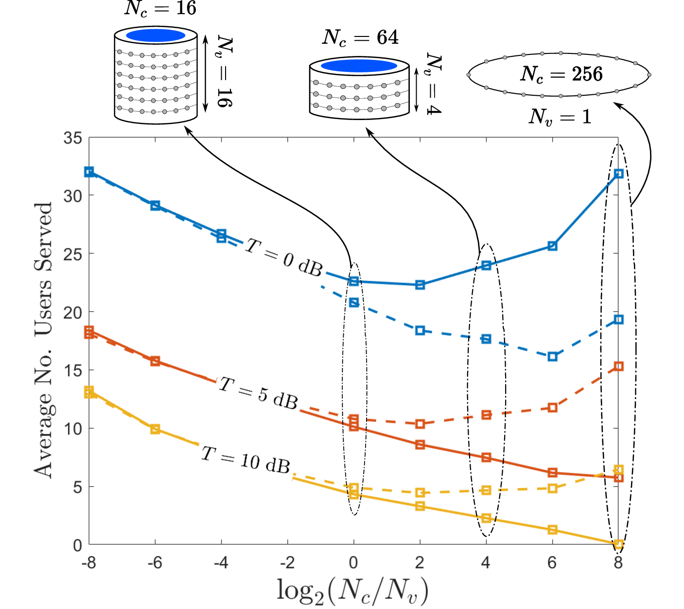
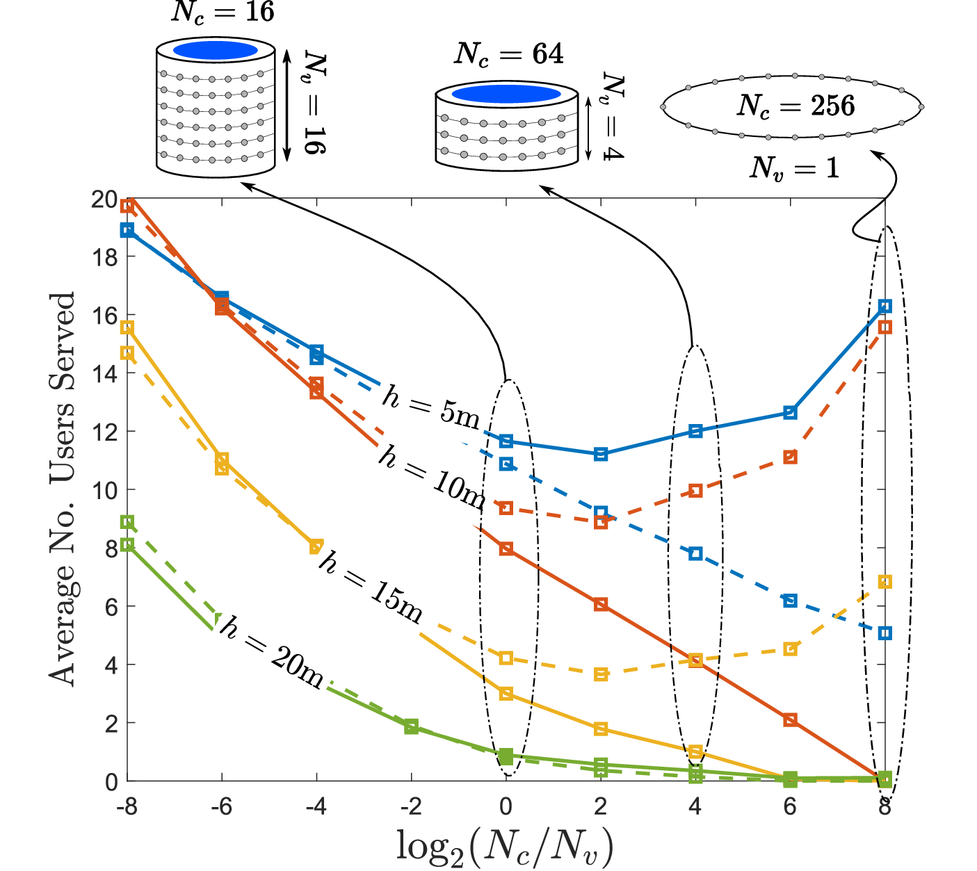
Figure 5 illustrates $\bar{P}_{s}$ vs. the antennas ratio $\log_{2}(N_{c}/N_{v})$, varying the SINR threshold $[T]_{dB}=\{0,5,10\}$ for small and large path-loss exponents $2b=\{2,3.6\}$. It can be seen that in the given scenario, by increasing the threshold $T$, UCAperforms worse. Note that in this setup, the UEs are very dense ($\lambda=5\times 10^{-2}\,m^{-2}$). It can be shown that for smaller UE densities, UCAoutperforms the UcylA. Fig. 6 shows a similar example of $\bar{P}_{s}$ vs. the antennas ratio $\log_{2}(N_{c}/N_{v})$, fixing the threshold $[T]_{dB}=5$ and varying the AP height $h=\{5,10,15,20\}\,m$. Clearly by increasing the AP height, the usage of UcylAbecomes more advantageous in terms of $\bar{P}_{s}$ and it is more meaningful to use vertical beamforming, while for smaller heights it is preferable to use a larger circular array. However, it can be observed that in this scenario where UEs are dense, the service probability in general decreases by increasing the height. Thus, it is preferable to use an AP with smaller height.
Fig. 7 shows the effect of UEs density $\lambda$. It is seen that for areas that are not so dense, a UCAis mildly preferable. However for more dense areas, a UcylAwould be more preferable depending on different parameters. It can be shown that changing every one of the above-mentioned parameters affects the shape of the $\bar{P}_{s}$ curves. Furthermore, the constraint of ground UEs is also responsible for results. UcylAs are favored in case UEs have arbitrary heights (usually indoor UEs are at arbitrary heights, while in high frquencies we target, penetration loss is too high).

A pragmatic conclusion from these evaluations is that for most real-life scenarios where UEs densities are not too high, it is beneficial to invest in UCAarrangement rather than UcylA. There are two reasons supporting this result: i) the most powerful interferers are in the vicinity of the AP, while the minimum separable angle by the ULA is $\Delta\theta_{min}\approx\frac{\lambda}{N_{v}d_{v}cos(\theta_{0})}$, where $d_{v}$ is the vertical inter-element spacing, and $\theta_{0}$ is the target elevation; ii) even if the resolution was not angle dependent, dividing the whole elevation plane into small portions of same width is emphasizing the same way to near and to far UEs, while the most powerful UEs are closer ones. In the rest of the numerical examples in the paper, we focus on the usage of UCA, since the target threshold used is set to $[T]_{dB}=0$ and the interferers’ density used are not extremely high, that justifies the usage of a UCAover UcylA.
Remark 3: Note that although the left most parts of the curves (i.e. corresponding to a ULAor a very tall UcylA) are shown in the figures, in practice they are not feasible to deploy. Therefore, one might consider the range $N_{c}>N_{v}/8$ as practical solution.

Previous studies and measurement campaigns [45], have shown that the NLOS clusters of rays are present in mmWcommunications where they form sparse multipath faded channels. These paths can increase the amount of interference, but at the same time would lead to more useful signal received in the case of coherent reception of signal. On the other hand, diversity is an efficient way to compensate the blockage and to increase the reliability of communication systems.

Let $L$ be the total number of paths that the signal arrives from the user of interest to the same AP, the $L\times 1$ set of signals $\mathbf{y}=[y_{1},y_{2},...,y_{L}]^{T}$ after the multi-beam beamforming to each of the paths from the user of interest transmitting $x$ is

$$\mathbf{y}=\mathbf{h}x+{\boldsymbol{\iota}}+{\mathbf{w}}$$

(37)

where $[\mathbf{h}]_{\ell}=h_{\ell}=\beta_{o,\ell}/D_{\ell}^{b}$ for distance $D_{\ell}=(R_{o,\ell}^{2}+h^{2})^{1/2}$ corresponding to the $\ell$th paths of arrival (in case $\ell=1$ it is the direct LOS link and $R_{o,1}=R_{o}$ is the geometric distance between the user of interest, while the distances for NLOS links are modelled later but $R_{o,\ell}\geq R_{o}$. The ensemble of the aggregated interference amplitudes from the PPP distributed interferers is ${\boldsymbol{\iota}}=[{\iota}_{1},{\iota}_{2},...,{\iota}_{L}]^{T}$ that are independent and identically distributed (iid) random variables are obtained from a set of $L$ beamforming toward the distinct angles $\phi_{o,1},\phi_{o,2},...,\phi_{o,L}$ for LOS ($\phi_{o,1}$) and NLOS ($\phi_{o,2},...,\phi_{o,L}$) of the user of interest, so that adapting 4 to this case with multipath for interference is:

$$\iota=\sum_{i=1}^{\infty}\sum_{\ell=1}^{L}\frac{\beta_{i,\ell}}{\left({R_{i,\ell}^{2}+h^{2}}\right)^{\frac{b}{2}}}G_{c}(\phi_{i,\ell})x_{i,\ell}.$$

(38)

This assumption is justified by the interfering ray-paths on every beamforming that have different attenuations and phase shifts, thus independent. $\mathbf{w}=[{w}_{1},{w}_{2},...,{w}_{L}]^{T}$ is the collection of noise amplitudes. The LOS/NLOS links are shown in Fig. 10 and using the Weyl model (similar to Saleh-Valenzuela [46] adapted for mmW [47, 48]) where the indirect NLOS paths from the transmitter are reflected from a secondary point which is uniformly distributed around a circle with radius $d$ around each of the transmitter’s location. Usually, at high frequencies, there are not many NLOS paths so that typically are $L=2-3$ [49, 50], [51]. The receiver for $L$ paths, possibly with different (and likely delay-resolvable for mmW and sub-THz system with large bandwidth) delays is expected to combine to maximize the service probability. If using the Maximal Ratio Combining (MRC)combiner for the $L$ paths related to the user of interest affected by the interference powers $I_{\ell}=|{\iota}_{\ell}|^{2}$, one gets the following service probability analysis (see Appendix B for derivation and specific MRCnotation):

$${P}_{MRC}=\mathbb{P}_{I}\left(\sum_{\ell=1}^{L}{\alpha_{\ell}{I}_{\ell}}<\frac{1}{T}\left(\sum_{\ell=1}^{L}\frac{|\beta_{\ell}|^{2}}{\bar{{I}}_{\ell}^{2}\,D_{\ell}^{2b}}\right)^{2}\right).$$

(39)

where $|\beta_{\ell}|^{2}$ is the fluctuation for the signal from the user of interest from $\ell$th path, and the distribution of total interference $I_{MRC}=\sum_{\ell=1}^{L}{\alpha_{\ell}{I}_{\ell}}$ follows from the CFfor iid interferers over the L-beamformers:

$$\Psi_{{I_{MRC}}}(\omega)=\prod_{\ell=1}^{L}\Psi_{{I}}(a_{\ell}\omega).$$

(40)

References

- [1] N. Panwar, S. Sharma, and A. K. Singh, “A survey on 5g: The next generation of mobile communication,” Physical Communication, vol. 18, pp. 64–84, 2016, special Issue on Radio Access Network Architectures and Resource Management for 5G. [Online]. Available: https://www.sciencedirect.com/science/article/pii/S1874490715000531
- [2] T. T. S. Rappaport, S. Sun, R. Mayzus, H. Zhao, Y. Azar, K. Wang, G. N. Wong, J. K. Schulz, M. Samimi, and F. Gutierrez, “Millimeter wave mobile communications for 5g cellular: It will work!” IEEE Access, vol. 1, pp. 335–349, 2013.
- [3] F. Qamar, M. U. A. Siddiqui, M. N. Hindia, R. Hassan, and Q. N. Nguyen, “Issues, challenges, and research trends in spectrum management: A comprehensive overview and new vision for designing 6g networks,” Electronics, vol. 9, no. 9, 2020. [Online]. Available: https://www.mdpi.com/2079-9292/9/9/1416
- [4] L. Azpilicueta, P. Lopez, J. Zuniga-Mejia, M. Celaya, F. A. Rodríguez, C. Vargas, E. Aguirre, D. G. Michelson, and F. Falcone, “Fifth-generation (5g) mmwave spatial channel characterization for urban environments system analysis,” Sensors, vol. 20, no. 18, 2020.
- [5] M. Ikram, K. Sultan, M. F. Lateef, and A. S. M. Alqadami, “A road towards 6g communication;a review of 5g antennas, arrays, and wearable devices,” Electronics, vol. 11, no. 1, 2022. [Online]. Available: https://www.mdpi.com/2079-9292/11/1/169
- [6] R. Singh, W. Lehr, D. Sicker, and K. Huq, “Beyond 5g: The role of thz spectrum,” SSRN Electronic Journal, 01 2019.
- [7] K. Dong, M. Mizmizi, D. Tagliaferri, and U. Spagnolini, “Vehicular blockage modelling and performance analysis for mmwave v2v communications,” 2021.
- [8] H. Q. Ngo, E. G. Larsson, and T. L. Marzetta, “Energy and spectral efficiency of very large multiuser mimo systems,” IEEE Transactions on Communications, vol. 61, no. 4, pp. 1436–1449, 2013.
- [9] M. Z. Win, P. C. Pinto, and L. A. Shepp, “A mathematical theory of network interference and its applications,” Proceedings of the IEEE, vol. 97, no. 2, pp. 205–230, Feb 2009.
- [10] M. Baianifar, S. Khavari, S. M. Razavizadeh, and T. Svensson, “Impact of user height on the coverage of 3d beamforming-enabled massive mimo systems,” in 2017 IEEE 28th Annual International Symposium on Personal, Indoor, and Mobile Radio Communications (PIMRC), Oct 2017, pp. 1–5.
- [11] A. Mouradian, “Modeling dense urban wireless networks with 3d stochastic geometry,” Performance Evaluation, vol. 121-122, pp. 1 – 17, 2018. [Online]. Available: http://www.sciencedirect.com/science/article/pii/S0166531617300287
- [12] H. ElSawy, A. Sultan-Salem, M. Alouini, and M. Z. Win, “Modeling and analysis of cellular networks using stochastic geometry: A tutorial,” IEEE Communications Surveys Tutorials, vol. 19, no. 1, pp. 167–203, Firstquarter 2017.
- [13] H. ElSawy, E. Hossain, and M. Haenggi, “Stochastic geometry for modeling, analysis, and design of multi-tier and cognitive cellular wireless networks: A survey,” IEEE Communications Surveys Tutorials, vol. 15, no. 3, pp. 996–1019, Third 2013.
- [14] S. Weber and J. G. Andrews, “Transmission capacity of wireless networks,” CoRR, vol. abs/1201.0662, 2012. [Online]. Available: http://arxiv.org/abs/1201.0662
- [15] T. Bai and R. W. Heath, “Analyzing uplink sinr and rate in massive mimo systems using stochastic geometry,” IEEE Transactions on Communications, vol. 64, no. 11, pp. 4592–4606, Nov 2016.
- [16] M. D. Renzo, A. Guidotti, and G. E. Corazza, “Average rate of downlink heterogeneous cellular networks over generalized fading channels: A stochastic geometry approach,” IEEE Transactions on Communications, vol. 61, no. 7, pp. 3050–3071, July 2013.
- [17] M. Filo, C. H. Foh, S. Vahid, and R. Tafazolli, “Performance impact of antenna height in ultra-dense cellular networks,” in 2017 IEEE International Conference on Communications Workshops (ICC Workshops), 2017, pp. 429–434.
- [18] J. Liu, M. Sheng, K. Wang, and J. Li, “The impact of antenna height difference on the performance of downlink cellular networks,” 2017.
- [19] A. Al-Hourani, S. Kandeepan, and S. Lardner, “Optimal lap altitude for maximum coverage,” IEEE Wireless Communications Letters, vol. 3, no. 6, pp. 569–572, Dec 2014.
- [20] K. Yoshikawa, K. Yamamoto, T. Nishio, and M. Morikura, “Grid-based exclusive region design for 3d uav networks: A stochastic geometry approach,” IEEE Access, vol. 7, pp. 103 806–103 814, 2019.
- [21] M. M. Azari, F. Rosas, A. Chiumento, and S. Pollin, “Coexistence of terrestrial and aerial users in cellular networks,” in 2017 IEEE Globecom Workshops (GC Wkshps), Dec 2017, pp. 1–6.
- [22] E. Chu, J. M. Kim, and B. C. Jung, “Interference modeling and analysis in 3-dimensional directional uav networks based on stochastic geometry,” ICT Express, 2019.
- [23] D. Maamari, N. Devroye, and D. Tuninetti, “Coverage in mmwave cellular networks with base station co-operation,” IEEE Transactions on Wireless Communications, vol. 15, no. 4, pp. 2981–2994, April 2016.
- [24] M. Cheng, J. Wang, Y. Wu, X. Xia, K. Wong, and M. Lin, “Coverage analysis for millimeter wave cellular networks with imperfect beam alignment,” IEEE Transactions on Vehicular Technology, vol. 67, no. 9, pp. 8302–8314, Sep. 2018.
- [25] J. G. Andrews, F. Baccelli, and R. K. Ganti, “A tractable approach to coverage and rate in cellular networks,” IEEE Transactions on Communications, vol. 59, no. 11, pp. 3122–3134, November 2011.
- [26] T. Alwajeeh, P. Combeau, R. Vauzelle, and A. Bounceur, “A high-speed 2.5d ray-tracing propagation model for microcellular systems, application: Smart cities,” in 2017 11th European Conference on Antennas and Propagation (EUCAP), 2017, pp. 3515–3519.
- [27] Z. Liu, L.-X. Guo, and W. Tao, “Full automatic preprocessing of digital map for 2.5d ray tracing propagation model in urban microcellular environment,” Waves in Random and Complex Media, vol. 23, 08 2013.
- [28] X. Yu, J. Zhang, M. Haenggi, and K. B. Letaief, “Coverage analysis for millimeter wave networks: The impact of directional antenna arrays,” IEEE Journal on Selected Areas in Communications, vol. 35, no. 7, pp. 1498–1512, July 2017.
- [29] L. Josefsson and P. Persson, Conformal array antenna theory and design. John wiley & sons, 2006, vol. 29.
- [30] J. G. Andrews, T. Bai, M. N. Kulkarni, A. Alkhateeb, A. K. Gupta, and R. W. Heath, “Modeling and analyzing millimeter wave cellular systems,” IEEE Transactions on Communications, vol. 65, no. 1, pp. 403–430, Jan 2017.
- [31] S. Stergiopoulos and A. C. Dhanantwari, “Implementation of adaptive processing in integrated active-passive sonars with multi-dimensional arrays,” in 1998 IEEE Symposium on Advances in Digital Filtering and Signal Processing. Symposium Proceedings (Cat. No.98EX185), June 1998, pp. 62–66.
- [32] S. M. Razavizadeh, M. Ahn, and I. Lee, “Three-dimensional beamforming: A new enabling technology for 5g wireless networks,” IEEE Signal Processing Magazine, vol. 31, no. 6, pp. 94–101, Nov 2014.
- [33] N. Wu, F. Zhu, and Q. Liang, “Evaluating spatial resolution and channel capacity of sparse cylindrical arrays for massive mimo,” IEEE Access, vol. 5, pp. 23 994–24 003, 2017.
- [34] H. L. V. Trees, Detection, Estimation, and Modulation Theory, Part III: Radar Sonar Signal Processing and Gaussian Signals in Noise. John Wiley & Sons, INC., 2001.
- [35] U. Spagnolini, Statistical Signal Processing in Engineering. John Wiley & Sons, Incorporated, 2018. [Online]. Available: https://books.google.it/books?id=yTg9swEACAAJ
- [36] H. Shokri-Ghadikolaei and C. Fischione, “Millimeter wave ad hoc networks: Noise-limited or interference-limited?” in 2015 IEEE Globecom Workshops (GC Wkshps), 2015, pp. 1–7.
- [37] M. Wildemeersch, T. Q. S. Quek, M. Kountouris, A. Rabbachin, and C. H. Slump, “Successive interference cancellation in heterogeneous networks,” IEEE Transactions on Communications, vol. 62, no. 12, pp. 4440–4453, Dec 2014.
- [38] A. Rabbachin, T. Q. S. Quek, H. Shin, and M. Z. Win, “Cognitive network interference,” IEEE Journal on Selected Areas in Communications, vol. 29, no. 2, pp. 480–493, February 2011.
- [39] X. Chen, D. W. K. Ng, W. Yu, E. G. Larsson, N. Al-Dhahir, and R. Schober, “Massive access for 5g and beyond,” 2020.
- [40] Y. Wen, S. Loyka, and A. Yongacoglu, “The impact of fading on the outage probability in cognitive radio networks,” in 2010 IEEE 72nd Vehicular Technology Conference - Fall, 2010, pp. 1–5.
- [41] J. Nolan, Stable distributions: models for heavy-tailed data. Birkhauser New York, 2003.
- [42] R. B. Davies, “Numerical inversion of a characteristic function,” Biometrika, vol. 60, no. 2, pp. 415–417, 1973.
- [43] N. G. Shephard, “From characteristic function to distribution function: a simple framework for the theory,” Econometric theory, vol. 7, no. 4, pp. 519–529, 1991.
- [44] M. A. T. Figueiredo and A. K. Jain, “Unsupervised learning of finite mixture models,” IEEE Transactions on Pattern Analysis and Machine Intelligence, vol. 24, no. 3, pp. 381–396, 2002.
- [45] M. R. Akdeniz, Y. Liu, M. K. Samimi, S. Sun, S. Rangan, T. S. Rappaport, and E. Erkip, “Millimeter wave channel modeling and cellular capacity evaluation,” IEEE Journal on Selected Areas in Communications, vol. 32, no. 6, pp. 1164–1179, 2014.
- [46] A. A. M. Saleh and R. Valenzuela, “A statistical model for indoor multipath propagation,” IEEE Journal on Selected Areas in Communications, vol. 5, no. 2, pp. 128–137, 1987.
- [47] Z. Peize, “Radio propagation and wireless coverage of lsaa-based 5g millimeter-wave mobile communication systems,” 06 2019.
- [48] M. Flament and A. Svensson, “Virtual cellular networks for 60 ghz wireless infrastructure,” 06 2003, pp. 1223 – 1227 vol.2.
- [49] M. K. Samimi and T. S. Rappaport, “3-d millimeter-wave statistical channel model for 5g wireless system design,” IEEE Transactions on Microwave Theory and Techniques, vol. 64, no. 7, pp. 2207–2225, 2016.
- [50] T. S. Rappaport, G. R. MacCartney, M. K. Samimi, and S. Sun, “Wideband millimeter-wave propagation measurements and channel models for future wireless communication system design,” IEEE Transactions on Communications, vol. 63, no. 9, pp. 3029–3056, 2015.
- [51] M. R. Akdeniz, Y. Liu, M. K. Samimi, S. Sun, S. Rangan, T. S. Rappaport, and E. Erkip, “Millimeter wave channel modeling and cellular capacity evaluation,” IEEE Journal on Selected Areas in Communications, vol. 32, no. 6, pp. 1164–1179, 2014.
- [52] A. Goldsmith, Wireless Communications. Cambridge University Press, 2005.
- [53] T. Bai, R. Vaze, and R. W. Heath, “Using random shape theory to model blockage in random cellular networks,” in 2012 International Conference on Signal Processing and Communications (SPCOM), 2012, pp. 1–5.
- [54] ——, “Analysis of blockage effects on urban cellular networks,” IEEE Transactions on Wireless Communications, vol. 13, no. 9, pp. 5070–5083, 2014.
- [55] I. K. Jain, R. Kumar, and S. S. Panwar, “The impact of mobile blockers on millimeter wave cellular systems,” IEEE Journal on Selected Areas in Communications, vol. 37, no. 4, pp. 854–868, 2019.
- [56] A. K. Gupta, J. G. Andrews, and R. W. Heath, “Macrodiversity in cellular networks with random blockages,” IEEE Transactions on Wireless Communications, vol. 17, no. 2, pp. 996–1010, 2018.
- [57] K. Venugopal and R. W. Heath, “Millimeter wave networked wearables in dense indoor environments,” IEEE Access, vol. 4, pp. 1205–1221, 2016.
- [58] W. G. Hofreiter, Integraltafel. Springer-Verlag Wien GMBH, 1950.