\normalbaroutside

2021

In this paper, we design an efficient, multi-stage image segmentation framework that incorporates a weighted difference of anisotropic and isotropic total variation (AITV). The segmentation framework generally consists of two stages: smoothing and thresholding, thus referred to as SaT. In the first stage, a smoothed image is obtained by an AITV-regularized Mumford-Shah (MS) model, which can be solved efficiently by the alternating direction method of multipliers (ADMM) with a closed-form solution of a proximal operator of the $\ell_{1}-\alpha\ell_{2}$ regularizer. Convergence of the ADMM algorithm is analyzed. In the second stage, we threshold the smoothed image by $K$ -means clustering to obtain the final segmentation result. Numerical experiments demonstrate that the proposed segmentation framework is versatile for both grayscale and color images, efficient in producing high-quality segmentation results within a few seconds, and robust to input images that are corrupted with noise, blur, or both. We compare the AITV method with its original convex TV and nonconvex TV ${}^{p}(0<p<1)$ counterparts, showcasing the qualitative and quantitative advantages of our proposed method.

An Efficient Smoothing and Thresholding Image Segmentation Framework with Weighted Anisotropic–Isotropic Total Variation

Kevin Bui Email: kevinb3@uci.edu Affiliation: Department of Mathematics, University of California, Irvine, Irvine, 92697-3875, CA, United States Yifei Lou Email: yflou@unc.edu Affiliation: Department of Mathematics, University of North Carolina, Chapel Hill, Chapel Hill, 27599, NC, United States Fredrick Park Email: fpark@whittier.edu Affiliation: Department of Mathematics & Computer Science, Whittier College, Whittier, 90602, CA, United States Jack Xin Email: jxin@math.uci.edu Affiliation: Department of Mathematics, University of California, Irvine, Irvine, 92697-3875, CA, United States

keywords

Image segmentation, Non-convex optimization, Mumford-Shah model, ADMM, proximal operator

1 Introduction

Image segmentation is a prevalent, challenging problem in computer vision, aiming to partition an image into several regions that represent specific objects of interest. Each partitioned region has similar features such as edges, colors, and intensities. One segmentation method is the Mumford-Shah (MS) model mumford1989optimal well-known for its robustness to noise. It finds the optimal piecewise-smooth approximation of an input image that incorporates region and boundary information to facilitate segmentation. Given a bounded, open set $\Omega\subset\mathbb{R}^{2}$ with Lipschitz boundary and an observed image $f:\Omega\rightarrow[0,1]$ , the MS model can be expressed as an energy minimization problem,

\displaystyle\begin{split}\min_{u,\Gamma}E_{MS}(u,\Gamma)\coloneqq&\frac{\lambda}{2}\int_{\Omega}(f-u)^{2}\;dx+\frac{\mu}{2}\int_{\Omega\setminus\Gamma}|\nabla u|^{2}\;dx+\text{Length}(\Gamma),\end{split}

(1)

where $\lambda,\mu>0$ are weighing parameters, $\Gamma\subset\Omega$ is a compact curve representing the boundaries separating disparate objects, and $u:\Omega\rightarrow\mathbb{R}$ is an approximation of $f$ that is smooth in $\Omega\setminus\Gamma$ but possibly discontinuous across $\Gamma$ . The middle term $\int_{\Omega\setminus\Gamma}|\nabla u|^{2}\;dx$ ensures that $u$ is piecewise smooth, or more specifically differentiable on $\Omega\setminus\Gamma$ . The last term “ $\text{Length}(\Gamma)$ ” measures the perimeter of $\Gamma$ that can be mathematically expressed as $\mathcal{H}^{1}(\Gamma)$ , which is the 1-dimensional Hausdorff measure in $\mathbb{R}^{2}$ bar2011mumford. It is challenging to solve for the minimization problem (1) due to its nonconvex nature and difficulties in discretizing the unknown set of boundaries. Pock et al. pock2009algorithm proposed a convex relaxation of (1) together with an efficient primal-dual algorithm. For the boundary issue, one early attempt involved a sequence of (local) elliptic variational problems ambrosio1990approximation to approximate the energy functional (1). Later, nonlocal approximations were adopted in gobbino1998finite; chambolle1999finite and a finite element approximation was developed in chambolle1999discrete.

By relaxing $u$ from piecewise smooth to piecewise constant, Chan and Vese (CV) chan-vese-2001 proposed a two-phase model to segment the image domain $\Omega$ into two regions that are inside and outside of the curve $\Gamma$ . The curve can be represented by a level-set function $\phi$ that is Lipschitz continuous and satisfies

\displaystyle\begin{cases}\phi(x)>0&\text{ if }x\text{ is inside }\Gamma,\\ \phi(x)=0&\text{ if }x\text{ is at }\Gamma,\\ \phi(x)<0&\text{ if }x\text{ is outside }\Gamma.\end{cases}

The Heaviside function $H(\phi)$ is defined by $H(\phi)=1$ if $\phi\geq 0$ and $H(\phi)=0$ otherwise. The CV model is given by

\displaystyle\begin{split}\min_{c_{1},c_{2},\phi}E_{CV}(c_{1},c_{2},\phi)&\coloneqq\lambda\int_{\Omega}|f-c_{1}|^{2}H(\phi)\;dx+\lambda\int_{\Omega}|f-c_{2}|^{2}(1-H(\phi))\;dx\\ &+\nu\int_{\Omega}|\nabla H(\phi)|\;dx,\end{split}

(2)

where $\lambda,\nu$ are two positive parameters and $c_{1},c_{2}\in\mathbb{R}$ are mean intensity values of the two regions. Originally, the CV model (2) was solved by finite difference methods chan2000active; getreuer2012chan. Later Chan et al. chan-esedoglu-nikolova-2004 formulated a convex relaxation of CV so that it can be solved by convex optimization techniques such as split Bregman goldstein2009split; goldstein2010geometric, alternating direction method of multipliers (ADMM) boyd2011distributed, and primal-dual hybrid gradient (PDHG) esser2010general; chambolle-pock-2011. As an alternative to the level-set formulation (2), a diffuse-interface approximation to the CV model was considered in esedog2006threshold, which can be solved efficiently by the Merrimen-Bence-Osher scheme merriman1994motion. The (two-phase) CV model can be naively extended to the multiphase segmentation vese2002multiphase but with a limitation that it can only deal with power-two number of segmentation regions. The multiphase CV model was later combined with fuzzy membership functions li2010multiphase in order to segment arbitrary number of regions.

Another approach of finding a piecewise-constant solution to the MS model is the smoothing-and-thresholding (SaT) framework cai2013two. In SaT, one first finds a smoothed image $u$ by solving a convex variant of the MS model:

\displaystyle\begin{split}\min_{u}&\frac{\lambda}{2}\int_{\Omega}(f-Au)^{2}\;dx+\frac{\mu}{2}\int_{\Omega}|\nabla u|^{2}\;dx+\int_{\Omega}|\nabla u|\;dx,\;\end{split}

(3)

where $\lambda>0,\mu>0,$ and $A$ is a linear operator. Specifically, $A$ is the identity operator if one wants to segment a noisy image $f$ , while it can be a blurring operator for the desire of segmenting a blurry and noisy image $f$ . The middle term $\int_{\Omega}|\nabla u|^{2}\;dx$ extends the piecewise-smooth regularization $\int_{\Omega\setminus\Gamma}|\nabla u|^{2}\;dx$ in (1) to the entire image domain $\Omega$ . The last term $\int_{\Omega}|\nabla u|\;dx$ is the total variation (TV) that approximates the length term in (1) based on the coarea formula chan-esedoglu-nikolova-2004. After obtaining a piecewise-smooth approximation, one segments the image domain into $K$ regions by thresholding $u$ with $K-1$ appropriately selected values. SaT has several advantages over the MS model (1) and the CV model (2). First, the smoothing stage involves a strictly convex problem (3) to guarantee a unique solution that can be found by numerous convex optimization algorithms. Second, the thresholding stage allows for segmenting any number of regions via a clustering algorithm such as $K$ -means clustering hartigan1979ak; arthur07. Lastly, thresholding is independent of smoothing; in other words, thresholding can be adjusted to obtain a visually appealing segmentation without going back to smoothing again. SaT was adapted to segment images corrupted by Poisson or multiplicative Gamma noise chan2014two. For color images, SaT extended to quaternion space wu2022efficient or evolved into the “smoothing, lifting, and thresholding” (SLaT) framework cai2017three. The additional lifting stage in SLaT adds the Lab (perceived lightness, red-green and yellow-blue) color space to provide more discriminatory information than the conventional RGB color space with correlated color channels. The idea of lifting can also improve image segmentation of grayscale images whose pixel intensities vary dramatically, referred to as intensity inhomogeneity. Traditional methods that deal with inhomogeneity include preprocessing hou2006review and intensity correction li2008minimization; wang2010efficient. By generating an additional image channel li2020three, SaT/SLaT yields better segmentation results for grayscale images that suffer from intensity inhomogeneity.

Note that the convex approximation of the length term in (1) by $\int_{\Omega}|\nabla u|\;dx$ in (3) is not optimal, since the Hausdorff measure is nonconvex. For a better approximation, Wu et al. wu2021two adopted a nonconvex term $\int_{\Omega}|\nabla u|^{p}\;dx$ for $(0<p<1),$ referred to as $\text{TV}^{p}$ , leading to a nonconvex problem,

\displaystyle\begin{split}\min_{u}&\frac{\lambda}{2}\int_{\Omega}(f-Au)^{2}\;dx+\frac{\mu}{2}\int_{\Omega}|\nabla u|^{2}\;dx+\int_{\Omega}|\nabla u|^{p}\;dx.\end{split}

(4)

If $p=1,$ $\text{TV}^{p}$ becomes the TV model. Generally, $\text{TV}^{p}$ outperforms TV in image restoration and segmentation chen2012non; hintermuller2013nonconvex; lanza2016constrained; zeng2018edge; li2020tv. The $\text{TV}^{p}$ regularization originated from the $\ell_{p}$ quasinorm, which is more effective than the convex $\ell_{1}$ norm in recovering sparse signals from an underdetermined linear system chartrand2008iteratively; xu2012l_. Recently, a series of work lou2015computational; lou-2015-cs; yin2015minimization has demonstrated through experiments that the nonconvex regularizer $\ell_{1}-\ell_{2}$ outperforms $\ell_{1}$ and $\ell_{p}$ when the linear system is highly coherent. The $\ell_{1}-\ell_{2}$ model can be generalized to $\ell_{1}-\alpha\ell_{2}$ for $\alpha\in[0,1]$ to allow for sparsity control via the parameter $\alpha$ . Theoretical analyses of the $\ell_{1}-\alpha\ell_{2}$ family have been investigated in ding2019regularization; yin2015minimization; ge2021new; li2020 that justify its superior performances. When applying $\ell_{1}-\alpha\ell_{2}$ on the image gradient, Lou et al. lou-2015 proposed a weighted difference of anisotropic and isotropic TV (AITV) that yields better results over TV and $\text{TV}^{p}$ for image denoising and deconvolution. AITV is robust against impulsive noise for image reconstruction li2020, and it yields satisfactory segmentation results in the CV model and the fuzzy region competition model bui2020weighted. Recently, an AITV-based segmentation model was discussed in wu2022image. However, these models are solved by a difference-of-convex algorithm (DCA) le2018dc; tao-1997; tao-1998 that requires solving a TV-type subproblem iteratively, thus being computationally expensive.

In this paper, we propose an efficient ADMM framework to solve the AITV variant of (3) and demonstrate its efficiency and effectiveness in the SaT/SLaT framework through various numerical experiments. The efficiency lies in the closed-form solution louY18 of the proximal operator for $\ell_{1}-\alpha\ell_{2}$ to avoid nested loops in DCA as considered in bui2020weighted; wu2022image. The main contributions of this paper are summarized as follows:

1.

We provide model analysis such as coerciveness and the existence of global minimizers for the AITV-regularized variant of (3).
2.

We develop an efficient ADMM algorithm for minimizing the AITV-based MS model based on the proximal operator of $\ell_{1}-\alpha\ell_{2}$ with a convergence guarantee.
3.

We conduct extensive numerical experiments to showcase that the SaT/SLaT framework with AITV regularization is a competitive segmentation method, especially using our proposed ADMM algorithm. The segmentation framework is robust to noise, blur, and intensity inhomogeneity.
4.

We demonstrate experimentally that the proposed ADMM framework is significantly more efficient than DCA used in bui2020weighted; wu2022image in producing segmentation results of comparable or even better quality.

The paper is organized as follows. Section 2 summarizes mathematical notations and reviews the SaT/SLaT framework. Section 3 provides analysis of the AITV-regularized MS model that can be solved by ADMM. Convergence analysis of the algorithm subsequently follows. Section 4 presents extensive experiments on various grayscale and color images, comparing the AITV SaT/SLaT framework to other state-of-the-art segmentation methods to demonstrate the effectiveness of the proposed approaches. Lastly, we conclude the paper in Section 5.

2 Preliminaries

2.1 Notations

For simplicity, we adopt the discrete notations for images and mathematical models. Without loss of generality, an image is represented as an $M\times N$ matrix, so the image domain is $\Omega=\{1,2,\ldots,M\}\times\{1,2,\ldots,N\}$ . Then we denote $X\coloneqq\mathbb{R}^{M\times N}$ . We adopt the linear index for 2D image, where for $u\in X$ , we have $u_{i,j}\in\mathbb{R}$ be the $((i-1)M+j)$ th component of $u$ . The gradient operator $\nabla:X\rightarrow X\times X$ is denoted by $\nabla u=(\nabla_{x}u,\nabla_{y}u)$ with $\nabla_{x}$ and $\nabla_{y}$ being the horizontal and vertical forward difference operators, respectively, with the periodic boundary condition. Specifically, the $(i,j)$ th entry of $\nabla u$ is defined by

\displaystyle(\nabla u)_{i,j}=\begin{bmatrix}(\nabla_{x}u)_{i,j}\\ (\nabla_{y}u)_{i,j}\end{bmatrix},

where

\displaystyle(\nabla_{x}u)_{i,j}=\begin{cases}u_{i,j}-u_{i,j-1}&\text{ if }2\leq j\leq N,\\ u_{i,1}-u_{i,N}&\text{ if }j=1\end{cases}

and

\displaystyle(\nabla_{y}u)_{i,j}=\begin{cases}u_{i,j}-u_{i-1,j}&\text{ if }2\leq i\leq M,\\ u_{1,j}-u_{M,j}&\text{ if }i=1.\end{cases}

For $p=(p_{x},p_{y})\in X\times X$ , its $((i-1)M+j)$ th component is $p_{i,j}=\begin{bmatrix}(p_{x})_{i,j}\\ (p_{y})_{i,j}\end{bmatrix}\in\mathbb{R}^{2}$ . We define the following norms on $X\times X$ :

	$\displaystyle\\|p\\|_{1}$	$\displaystyle=\sum_{i=1}^{M}\sum_{j=1}^{N}\left(\|(p_{x})_{i,j}\|+\|(p_{y})_{i,j}\|\right),$
	$\displaystyle\\|p\\|_{2}$	$\displaystyle=\sqrt{\sum_{i=1}^{M}\sum_{j=1}^{N}\|(p_{x})_{i,j}\|^{2}+\|(p_{y})_{i,j}\|^{2}},$
	$\displaystyle\\|p\\|_{2,1}$	$\displaystyle=\displaystyle\sum_{i=1}^{M}\sum_{j=1}^{N}\sqrt{(p_{x})_{i,j}^{2}+(p_{y})_{i,j}^{2}}.$

Lastly, the proximal operator for a function $f:\mathbb{R}^{n}\rightarrow\mathbb{R}\cup\{+\infty\}$ at $y\in\mathbb{R}^{n}$ is given by

\displaystyle\text{prox}_{f}(y)=\argmin_{x\in\mathbb{R}^{n}}f(x)+\frac{1}{2}\|x-y\|_{2}^{2}.

2.2 Review of SaT/SLaT

Both SaT and SLaT frameworks consist of two general steps: (1) smoothing to extract a piecewise-smooth approximation of a given image and (2) thresholding to segment the regions via $K$ -means clustering. SLaT has an intermediate stage called lifting, which generates additional color channels as opposed to the RGB color space for the smoothed image. More details for each stage are described below.

2.2.1 First Stage: Smoothing

Let $f=(f_{1},\ldots,f_{d})\in X^{d}$ , where $d$ represents the number of channels in the image $f$ . For example, when the image $f$ is grayscale, we have $d=1$ , and when it is color, we have $d=3$ . In general, $f$ can be a multichannel image. Some of its channels could be generated from the original image to provide more information for segmentation. For example, the intensity inhomogeneity image li2020three is generated as an additional channel that quantifies the amount of intensity inhomogeneity in the original image.

The discretized model of (3) for each channel $\ell=1,\ldots,d$ can be expressed as

\displaystyle\begin{split}\min_{u_{\ell}}\frac{\lambda}{2}\|f_{\ell}-Au_{\ell}\|_{2}^{2}+\frac{\mu}{2}\|\nabla u_{\ell}\|_{2}^{2}+&\|\nabla u_{\ell}\|_{2,1},\end{split}

(5)

where $\lambda>0,\mu>0$ and $\|\nabla u_{\ell}\|_{2}^{2}$ is a smoothing term to reduce the staircase effects caused by the isotropic TV $\|\nabla u_{\ell}\|_{2,1}$ . We assume the same pair of parameters $(\lambda,\mu)$ across channels. In summary, we obtain a smooth approximation $u_{\ell}$ for each channel $f_{\ell}$ by solving (5).

2.2.2 Intermediate Stage: Lifting

For a color image $f=(f_{1},f_{2},f_{3})\in X^{3}$ , where $f_{1}$ , $f_{2}$ , and $f_{3}$ are the red, green, and blue channels, respectively, we can obtain $(u_{1},u_{2},u_{3})$ by applying the smoothing stage to each channel of $f$ . Instead of using $(u_{1},u_{2},u_{3})$ , SLaT transforms $(u_{1},u_{2},u_{3})$ into $(\bar{u}_{1},\bar{u}_{2},\bar{u}_{3})$ in the Lab space (perceived lightness, red-green, and yellow-blue) luong1993color and operates on a new vector-valued image $(u_{1},u_{2},u_{3},\bar{u}_{1},\bar{u}_{2},\bar{u}_{3})$ . The rationale is that RGB channels are highly correlated, while the Lab space relies on numerical color differences to approximate the color differences perceived by the human eye. As a result, $(u_{1},u_{2},u_{3},\bar{u}_{1},\bar{u}_{2},\bar{u}_{3})$ leads to better segmentation results compared to $(u_{1},u_{2},u_{3})$ .

2.2.3 Final Stage: Thresholding

After rescaling the image obtained after smoothing and/or lifting, we denote the resultant image by $u^{*}\in[0,1]^{D}$ . For example, we have $D=1$ when applying SaT to a grayscale image, and we have $D=6$ when applying SLaT to a color image. Suppose the number of segmented regions is given and denoted by $K$ . The thresholding stage applies $K$ -means clustering to the vector-valued image $u^{*}$ , providing $K$ centroids $c_{1},c_{2},\ldots,c_{K}$ as constant vectors. These centroids are used to form the regions

\displaystyle\Omega_{k}=\left\{(i,j)\in\Omega:\|u^{*}_{i,j}-c_{k}\|_{2}=\min_{1\leq\kappa\leq K}\|u_{i,j}^{*}-c_{\kappa}\|_{2}\right\},

for $k=1,\ldots,K$ such that $\Omega_{k}$ ’s are disjoint and $\bigcup_{k=1}^{K}\Omega_{k}=\Omega$ . Using the centroids and regions, we can obtain a piecewise-constant approximation of $f$ , denoted by

\displaystyle\tilde{f}=(\tilde{f}_{1},\ldots,\tilde{f}_{d})\text{ such that }\tilde{f}_{\ell}=\sum_{k=1}^{K}c_{k,\ell}\mathbbm{1}_{\Omega_{k}}\;\forall\ell=1,\ldots,d,

(6)

where $c_{k,\ell}$ is the $\ell$ th entry of $c_{k}$ and

\displaystyle\mathbbm{1}_{\Omega_{k}}=\begin{cases}1&\text{ if }(i,j)\in\Omega_{k},\\ 0&\text{ if }(i,j)\not\in\Omega_{k}.\end{cases}

Recall that $d=1$ when the image $f$ is grayscale and $d=3$ when it is color.

3 Smoothing with AITV Regularization

Refer to caption — (a) AITV SaT framework for grayscale image.

Input:

•

image $f=(f_{1},\ldots,f_{d})$
•

blurring operator $A$
•

fidelity parameter $\lambda>0$
•

smoothing parameter $\mu>0$
•

AITV parameter $\alpha\in[0,1]$
•

the number of regions in the image $K$

Output: Segmentation

\tilde{f}

Stage one: Compute

u_{\ell}

by solving (7) for

\ell=1,\ldots,d

. 1

Stage two: 2

if $f$ is a color image, i.e, $d=3$ then 3

Transfer

u=(u_{1},u_{2},u_{3})

into Lab space to obtain

(\bar{u}_{1},\bar{u}_{2},\bar{u}_{3})

and concatenate to form

(u_{1},u_{2},u_{3},\bar{u}_{1},\bar{u}_{2},\bar{u}_{3})

.else 4

Go to stage three. 5

Stage three: Apply

K

-means to obtain

\{(c_{l},\Omega_{k})\}_{k=1}^{K}

and compute

\tilde{f}

by (6).

Algorithm 1 AITV SaT/SLaT

We replace the isotropic TV in (5) by a weighted difference of anisotropic and isotropic TV, i.e.,

\displaystyle\begin{split}\min_{u}F(u)\coloneqq&\frac{\lambda}{2}\|f-Au\|_{2}^{2}+\frac{\mu}{2}\|\nabla u\|_{2}^{2}+\|\nabla u\|_{1}-\alpha\|\nabla u\|_{2,1},\end{split}

(7)

with $\lambda>0,\mu>0,\alpha\in[0,1].$ AITV is a more suitable alternative to TV (no matter whether it is anisotropic or isotropic) since TV typically fails to recover oblique edges birkholz2011unifying; condat2017discrete, which can be preserved by AITV bui2020weighted; lou-2015. To simplify notations, we omit the subscript $\ell$ in (5) because the smoothing model is applied channel by channel independently. We show that our model (7) admits a global solution in Section 3.1. To find a solution to (7), we describe in Section 3.2 the ADMM scheme with its convergence analysis conducted in Section 3.3. The overall AITV SaT/SLaT framework for segmentation is visualized in Figure 1 and summarized in Algorithm 1.

3.1 Model Analysis

In Theorem 3.1 we establish the existence of a global solution to (7) by showing that its objective function $F$ is coercive in Lemma 3.1.

Lemma 3.1.

If $\lambda>0,\mu>0,\alpha\in[0,1],$ and $\text{ker}(A)\cap\text{ker}(\nabla)=\{0\}$ , then $F$ defined in (7) is coercive.

Proof.

We prove by contradiction. Suppose there exists a sequence $\{u_{n}\}_{n=1}^{\infty}$ and a constant $C>0$ such that $\|u_{n}\|_{2}\rightarrow\infty$ and $F(u_{n})<C$ for all $n\in\mathbb{N}$ . We define a sequence $\{v_{n}\}_{n=1}^{\infty}$ where $v_{n}=\displaystyle\frac{u_{n}}{\|u_{n}\|_{2}}$ and thereby satisfies $\|v_{n}\|_{2}=1$ for all $n\in\mathbb{N}$ . Since $\{v_{n}\}_{n=1}^{\infty}$ is bounded, there exists a convergent subsequence $\{v_{n_{k}}\}_{k=1}^{\infty}$ such that $v_{n_{k}}\rightarrow v^{*}$ and $\|v^{*}\|_{2}=1$ .

It follows from $\|\nabla u\|_{2,1}\leq\|\nabla u\|_{1}$ that

\displaystyle F(u)

\displaystyle\geq\frac{\lambda}{2}\|Au-f\|_{2}^{2}+\frac{\mu}{2}\|\nabla u\|_{2}^{2}\geq\frac{\lambda}{2}(\|Au\|_{2}-\|f\|_{2})^{2}+\frac{\mu}{2}\|\nabla u\|_{2}^{2}.

Since $F(u_{n})<C$ , we have $\|\nabla u_{n}\|_{2}<\sqrt{\frac{2C}{\mu}}$ and $\|Au_{n}\|_{2}<\sqrt{\frac{2C}{\lambda}}+\|f\|_{2}$ . As a result, we have

	$\displaystyle\\|Av_{n_{k}}\\|_{2}$	$\displaystyle=\frac{\\|Au_{n_{k}}\\|_{2}}{\\|u_{n_{k}}\\|_{2}}<\frac{\sqrt{\frac{2C}{\lambda}}+\\|f\\|_{2}}{\\|u_{n_{k}}\\|_{2}}$
	$\displaystyle\\|\nabla v_{n_{k}}\\|_{2}$	$\displaystyle=\frac{\\|\nabla u_{n_{k}}\\|_{2}}{\\|u_{n_{k}}\\|_{2}}<\frac{\sqrt{2C}}{\sqrt{\mu}\\|u_{n_{k}}\\|_{2}}.$

After taking the limit $n_{k}\rightarrow\infty,$ we get $\|Av^{*}\|_{2}=0\text{ and }\|\nabla v^{*}\|_{2}=0$ , which implies that $v^{*}=0$ due to the assumption that $\text{ker}(A)\cap\text{ker}(\nabla)=\{0\}$ . However, it contradicts with $\|v^{*}\|_{2}=1$ , and hence $F$ is coercive. ∎

Theorem 3.1.

If $\lambda>0,\mu>0,\alpha\in[0,1],$ and $\text{ker}(A)\cap\text{ker}(\nabla)=\{0\}$ , then $F$ has a global minimizer.

Proof.

As $F$ is lower bounded by 0, it has a minimizing sequence $\{u_{n}\}_{n=1}^{\infty}$ . Without loss of generality, we assume $u_{1}=0$ . Since $F$ is coercive by Lemma 3.1, we have $F(u_{n})\leq F(0)<\infty$ , showing that $\{\|\nabla u_{n}\|_{1}\}_{n=1}^{\infty}$ and $\{\|Au_{n}\|_{2}\}_{n=1}^{\infty}$ are bounded. As $\text{ker}(A)\cap\text{ker}(\nabla)=\{0\}$ , we have $\{u_{n}\}_{n=1}^{\infty}$ shall be bounded. Then there exists a convergent subsequence $\{u_{n_{k}}\}_{k=1}^{\infty}$ such that $u_{n_{k}}\rightarrow u^{*}$ . Since $A$ and $\nabla$ are both bounded, linear operators, we have $Au_{n_{k}}\rightarrow Au^{*}$ and $\nabla u_{n_{k}}\rightarrow\nabla u^{*}$ . Since norms are continuous and thereby lower semi-continuous, we have

		$\displaystyle\\|\nabla u^{}\\|_{1}-\alpha\\|\nabla u^{}\\|_{2,1}\leq\liminf_{k\rightarrow\infty}\left(\\|\nabla u_{n_{k}}\\|_{1}-\alpha\\|\nabla u_{n_{k}}\\|_{2,1}\right),$
		$\displaystyle\\|\nabla u^{*}\\|_{2}^{2}\leq\liminf_{k\rightarrow\infty}\\|\nabla u_{n_{k}}\\|_{2}^{2},$
		$\displaystyle\\|Au^{*}-f\\|_{2}^{2}\leq\liminf_{k\rightarrow\infty}\\|Au_{n_{k}}-f\\|_{2}^{2}.$

Altogether, we obtain $F(u^{*})\leq\displaystyle\liminf_{k\rightarrow\infty}F(u_{n_{k}})$ , which implies that $u^{*}$ minimizes $F(u)$ . ∎

3.2 Numerical Scheme

We describe an efficient algorithm to minimize (7) via ADMM. In particular, we introduce an auxiliary variable $w=(w_{x},w_{y})\in X\times X$ and rewrite (7) into an equivalent constrained optimization problem

	$\displaystyle\min_{u,w}$	$\displaystyle\frac{\lambda}{2}\\|f-Au\\|_{2}^{2}+\frac{\mu}{2}\\|\nabla u\\|_{2}^{2}+\\|w\\|_{1}-\alpha\\|w\\|_{2,1}$		(8)
	$\displaystyle\text{s.t.}$	$\displaystyle\nabla u=w,$		(8)

where $w_{x}=\nabla_{x}u$ and $w_{y}=\nabla_{y}u$ . Then the corresponding augmented Lagrangian is expressed by

\displaystyle\begin{split}\mathcal{L}_{\delta}(u,w,z)\coloneqq&\frac{\lambda}{2}\|f-Au\|_{2}^{2}+\frac{\mu}{2}\|\nabla u\|_{2}^{2}+\|w\|_{1}-\alpha\|w\|_{2,1}\\ &+\langle z,\nabla u-w\rangle+\frac{\delta}{2}\|\nabla u-w\|_{2}^{2}\\ =&\frac{\lambda}{2}\|f-Au\|_{2}^{2}+\frac{\mu}{2}\|\nabla u\|_{2}^{2}+\|w\|_{1}-\alpha\|w\|_{2,1}\\ &+\frac{\delta}{2}\left\|\nabla u-w+\frac{z}{\delta}\right\|_{2}^{2}-\frac{1}{2\delta}\|z\|_{2}^{2},\end{split}

(9)

where $\delta>0$ is a penalty parameter and $z=(z_{x},z_{y})\in X\times X$ is a dual variable. The ADMM iterations proceed as follows:


$\displaystyle u_{t+1}$	$\displaystyle\in\displaystyle\argmin_{u}\mathcal{L}_{\delta_{t}}(u,w_{t},z_{t})$	(10a)
$\displaystyle w_{t+1}$	$\displaystyle\in\displaystyle\argmin_{w}\mathcal{L}_{\delta_{t}}(u_{t+1},w,z_{t})$	(10b)
$\displaystyle z_{t+1}$	$\displaystyle=z_{t}+\delta_{t}(\nabla u_{t+1}-w_{t+1})$	(10c)
$\displaystyle\delta_{t+1}$	$\displaystyle=\sigma\delta_{t},\;\sigma\geq 1.$	(10d)

Note that $\sigma=1$ reduces to the original ADMM framework boyd2011distributed. We consider an adaptive penalty parameter $\delta_{t}$ by choosing $\sigma>1$ . In fact, the parameter $\sigma>1$ controls the numerical convergence speed of the algorithm in the sense that a larger $\sigma$ leads to a fewer number of iterations the algorithm needs to run before satisfying a stopping criterion. However, if $\delta_{t}$ increases too quickly, the ADMM algorithm will numerically converge within a few iterations, which may yield a low-quality solution. Thus, a small $\sigma$ is recommended and we discuss its choice in experiments (Section 4).

Next we elaborate on how to solve the two subproblems (10a) and (10b). The subproblem (10a) is written as

\displaystyle\begin{split}u_{t+1}&\in\displaystyle\argmin_{u}\frac{\lambda}{2}\|f-Au\|_{2}^{2}+\frac{\mu}{2}\|\nabla u\|_{2}^{2}+\langle z_{t},\nabla u-w_{t}\rangle+\frac{\delta_{t}}{2}\|\nabla u-w_{t}\|_{2}^{2}.\end{split}

The first-order optimality condition of (10a) is given by

\displaystyle\begin{split}\left[\lambda A^{\top}A-(\mu+\delta_{t})\Delta\right]u_{t+1}=\lambda A^{\top}f+\delta_{t}\nabla^{\top}\left(w_{t}-\frac{z_{t}}{\delta_{t}}\right),\end{split}

where $\Delta=-\nabla^{\top}\nabla$ is the Laplacian operator. If $\text{ker}(A)\cap\text{ker}(\nabla)=\{0\}$ , then $\lambda A^{\top}A-(\mu+\delta_{t})\Delta$ is positive definite. By assuming the periodic boundary condition, $A^{\top}A$ and $\Delta$ are block circulant, so we can solve for $u_{t+1}$ via the fast Fourier transform $\mathcal{F}$ chan1996conjugate; ng1999fast; wang2008new. By the Convolution Theorem, the closed-form solution for $u_{t+1}$ is

\displaystyle\begin{split}u_{t+1}=\mathcal{F}^{-1}\left(\frac{\lambda\mathcal{F}(A)^{*}\circ\mathcal{F}(f)+\delta_{t}\mathcal{F}(\nabla)^{*}\circ\mathcal{F}\left(w_{t}-\displaystyle\frac{z_{t}}{\delta_{t}}\right)}{\lambda\mathcal{F}(A)^{*}\circ\mathcal{F}(A)-(\mu+\delta_{t})\mathcal{F}(\Delta)}\right),\end{split}

where $\mathcal{F}^{-1}$ is the inverse Fourier transform, $*$ denotes complex conjugate, $\circ$ denotes componentwise multiplication, and division is also componentwise.

Denote $w_{i,j}=\begin{bmatrix}(w_{x})_{i,j}\\ (w_{y})_{i,j}\end{bmatrix}\in\mathbb{R}^{2}$ as the $(i,j)$ th entry of $w$ . The subproblem (10b) can be expressed as

\displaystyle w_{t+1}\in\displaystyle\argmin_{w}\|w\|_{1}-\alpha\|w\|_{2,1}+\frac{\delta_{t}}{2}\left\|\nabla u_{t+1}+\frac{z_{t}}{\delta_{t}}-w\right\|_{2}^{2}.

Expanding (10b), we get

\displaystyle\begin{split}\argmin_{w}&\sum_{(i,j)\in\Omega}\Bigg(\|w_{i,j}\|_{1}-\alpha\|w_{i,j}\|_{2}+\frac{\delta_{t}}{2}\left\|(\nabla u_{t+1})_{i,j}+\frac{(z_{t})_{i,j}}{\delta_{t}}-w_{i,j}\right\|_{2}^{2}\Bigg),\end{split}

(11)

which shows that $w_{i,j}$ can be solved elementwise. Specifically, the optimal solution of $w_{i,j}\in\mathbb{R}^{2}$ is related to the proximal operator for $\ell_{1}-\alpha\ell_{2}$ defined by

\displaystyle\text{prox}(y;\alpha,\beta)\coloneqq\text{prox}_{\beta\left(\|\cdot\|_{1}-\alpha\|\cdot\|_{2}\right)}(y)=\argmin_{x}\|x\|_{1}-\alpha\|x\|_{2}+\frac{1}{2\beta}\|x-y\|_{2}^{2}.

(12)

The closed-form solution for (12) is given in Lemma 3.2 louY18. By comparing (11) and (12), the $w$ -update is given by $\forall(i,j)\in\Omega,$

\displaystyle\begin{split}(w_{t+1})_{i,j}=\text{prox}\left((\nabla u_{t+1})_{i,j}+\frac{(z_{t})_{i,j}}{\delta_{t}};\alpha,\frac{1}{\delta_{t}}\right).\end{split}

Lemma 3.2 (louY18).

Given $y\in\mathbb{R}^{n}$ , $\beta>0$ , and $\alpha\geq 0$ , the optimal solution to (12) can be discussed separately into the following cases:

1.

When $\|y\|_{\infty}>\beta$ , we have

$\displaystyle x^{*}=(\|\xi\|_{2}+\alpha\beta)\frac{\xi}{\|\xi\|_{2}},$

where $\xi=\sign(y)\circ\max(|y|-\beta,0)$ .
2.

When $(1-\alpha)\beta<\|y\|_{\infty}\leq\beta$ , then $x^{*}$ is a 1-sparse vector such that one chooses $i\in\displaystyle\argmax_{j}(|y_{j}|)$ and defines $x^{*}_{i}=\left(|y_{i}|+(\alpha-1)\beta\right)\sign(y_{i})$ and the rest of the elements equal to 0.
3.

When $\|y\|_{\infty}\leq(1-\alpha)\beta$ , then $x^{*}=0$ .

In summary, the ADMM scheme that minimizes (7) is presented in Algorithm 2.

Input:

•

image $f$
•

blurring operator $A$
•

fidelity parameter $\lambda>0$
•

smoothing parameter $\mu>0$
•

AITV parameter $\alpha\in[0,1]$
•

penalty parameter $\delta_{0}>0$
•

penalty multiplier $\sigma\geq 1$
•

relative error $\epsilon>0$

Output:

u_{t}

Initialize

u_{0},w_{0},z_{0}

.
Set

t=0

.
while $\frac{\|u_{t}-u_{t-1}\|_{2}}{\|u_{t}\|_{2}}>\epsilon$ do 1

	$\displaystyle u_{t+1}$	$\displaystyle=\mathcal{F}^{-1}\left(\frac{\lambda\mathcal{F}(A)^{}\circ\mathcal{F}(f)+\delta_{t}\mathcal{F}(\nabla)^{}\circ\mathcal{F}\left(w_{t}-\displaystyle\frac{z_{t}}{\delta_{t}}\right)}{\lambda\mathcal{F}(A)^{*}\circ\mathcal{F}(A)-(\mu+\delta_{t})\mathcal{F}(\Delta)}\right)$
	$\displaystyle(w_{t+1})_{i,j}$	$\displaystyle=\text{prox}\left((\nabla u_{t+1})_{i,j}+\frac{(z_{t})_{i,j}}{\delta_{t}};\alpha,\frac{1}{\delta_{t}}\right)\hskip 9.24994pt\forall(i,j)\in\Omega$
	$\displaystyle z_{t+1}$	$\displaystyle=z_{t}+\delta_{t}(\nabla u_{t+1}-w_{t+1})$
	$\displaystyle\delta_{t+1}$	$\displaystyle=\sigma\delta_{t}$
	$\displaystyle t$	$\displaystyle\coloneqq t+1$

Algorithm 2 ADMM for minimizing the AITV-Regularized smoothing model

3.3 Convergence Analysis

We aim to analyze the convergence for Algorithm 2. It is true that global convergence of ADMM has been established in deng2016global for certain classes of nonconvex optimization problems, but unfortunately it cannot be applied to our problem (8) since the gradient operator $\nabla$ is not surjective. Instead of global convergence, we manage to achieve weaker subsequential convergence for two cases: $\sigma=1$ and $\sigma>1$ . The proof of $\sigma>1$ is adapted from gu2017weighted; you2019nonconvex.

Before providing convergence results for ADMM, we provide a definition of subdifferential for general functions. For a function $h:\mathbb{R}^{n}\rightarrow\mathbb{R}\cup\{\infty\}$ , we denote the (limiting) subdifferential by $\partial{h(x)}$ (rockafellar2009variational, Definition 11.10), which is defined as a set

\displaystyle\begin{split}\partial h(x)=\{v\in\mathbb{R}^{n}:\exists\{(x_{t},v_{t})\}_{t=1}^{\infty}\text{ s.t. }x_{t}\rightarrow x,\;h(x_{t})\rightarrow h(x),\;v_{t}\in\hat{\partial}{h}(x_{t}),\text{and }v_{t}\rightarrow v\},\end{split}

with

\displaystyle\hat{\partial}h(x)=\left\{v\in\mathbb{R}^{n}:\liminf_{z\rightarrow x,z\neq x}\frac{h(z)-h(x)-\langle v,z-x\rangle}{\|z-x\|_{2}}\geq 0\right\}.

Since $\hat{\partial}h(x)\subset\partial{h}(x)$ where $h$ is finite on $x$ , the graph $x\mapsto\partial h(x)$ is closed clarke2013functional; rockafellar2009variational by definition:

\displaystyle v_{t}\in\partial h(x_{t}),\;x_{t}\rightarrow x,\;h(x_{t})\rightarrow h(x),\;

\displaystyle v_{t}\rightarrow v\implies v\in\partial h(x).

First, we present a lemma and a proposition whose proofs are delayed to the appendix.

Lemma 3.3.

Suppose that $\text{ker}(A)\cap\text{ker}(\nabla)=\{0\}$ . Let $\{(u_{t},w_{t},z_{t})\}_{t=1}^{\infty}$ be generated by (10a)-(10d) with $\sigma\geq 1$ . The following inequality holds:

\displaystyle\begin{split}&\mathcal{L}_{\delta_{t+1}}(u_{t+1},w_{t+1},z_{t+1})-\mathcal{L}_{\delta_{t}}(u_{t},w_{t},z_{t})\leq\frac{\sigma+1}{2\sigma^{t}\delta_{0}}\|z_{t+1}-z_{t}\|_{2}^{2}-\frac{\zeta}{2}\|u_{t+1}-u_{t}\|_{2}^{2},\end{split}

(13)

where $\zeta>0$ is the smallest eigenvalue of $\lambda A^{\top}A+(\mu+\delta_{0})\nabla^{\top}\nabla.$

Proposition 3.1.

Suppose that $\text{ker}(A)\cap\text{ker}(\nabla)=\{0\}$ . Let $\{(u_{t},w_{t},z_{t})\}_{t=1}^{\infty}$ be generated by (10a)-(10d). Assume one of the conditions holds:

•

$\sigma=1$ and $\displaystyle\sum_{i=0}^{\infty}\|z_{i+1}-z_{i}\|_{2}^{2}<\infty$ .
•

$\sigma>1$ .

Then we have the following statements:

(a)

The sequence $\{(u_{t},w_{t},z_{t})\}_{t=1}^{\infty}$ is bounded.
(b)

$u_{t+1}-u_{t}\rightarrow 0$ as $t\rightarrow\infty$ .

Proposition 3.1 reveals an advantage of using the adaptive penality parameter with $\sigma>1$ . For $\sigma=1$ , we require $\displaystyle\sum_{i=0}^{\infty}\|z_{i+1}-z_{i}\|_{2}^{2}<\infty$ in order for the iterates $\{(u_{t},w_{t},z_{t})\}_{t=1}^{\infty}$ of Algorithm 2 to be bounded and to satisfy the relative stopping criterion $\frac{\|u_{t}-u_{t-1}\|_{2}}{\|u_{t}\|_{2}}<\epsilon$ . The requirement $\displaystyle\sum_{i=0}^{\infty}\|z_{i+1}-z_{i}\|_{2}^{2}<\infty$ is no longer necessary if $\sigma>1$ .

Finally, we establish the subsequential convergence in Theorem 3.2 under stronger conditions compared to the ones in Proposition 3.1. These conditions are motivated by a series of works chang2016phase; chang2018total; jung2014variational; jung2017piecewise; li2016multiphase; li2020tv that proved the theoretical convergence of ADMM in solving TV-based inverse problems.

Theorem 3.2.

Let $\{(u_{t},w_{t},z_{t})\}_{t=1}^{\infty}$ be generated by (10a)-(10d). Assume one set of the following conditions holds:

•

$\sigma=1$ and $\displaystyle\sum_{i=0}^{\infty}\|z_{i+1}-z_{i}\|_{2}^{2}<\infty$ .
•

$\sigma>1$ , $\delta_{t}(w_{t+1}-w_{t})\rightarrow 0$ , and $z_{t+1}-z_{t}\rightarrow 0$ .

Then there exists a subsequence of $\{(u_{t},w_{t},z_{t})\}_{t=1}^{\infty}$ whose limit point $(u^{*},w^{*},z^{*})$ is a KKT point of (8) that satisfies


$\displaystyle 0$	$\displaystyle=\lambda A^{\top}(Au^{}-f)-\mu\Delta u^{}+\nabla^{\top}z^{*}$	(14a)
$\displaystyle z^{*}$	$\displaystyle\in\partial\left(\\|w^{}\\|_{1}-\alpha\\|w^{}\\|_{2,1}\right)$	(14b)
$\displaystyle\nabla u^{*}$	$\displaystyle=w^{*}.$	(14c)

Proof.

By Proposition 3.1, $\{(u_{t},w_{t},z_{t})\}_{t=1}^{\infty}$ is bounded, and hence there exists a subsequence that converges to a point $(u^{*},w^{*},z^{*})$ , denoted by $(u_{t_{k}},w_{t_{k}},z_{t_{k}})\rightarrow(u^{*},w^{*},z^{*}).$ Proposition 3.1 also establishes $\displaystyle\lim_{t\rightarrow\infty}u_{t+1}-u_{t}=0,$ which implies that $\displaystyle\lim_{k\rightarrow\infty}u_{t_{k}+1}=\lim_{k\rightarrow\infty}u_{t_{k}}=u^{*}.$ Either set of assumptions establishes $\displaystyle\lim_{k\rightarrow\infty}z_{t_{k}+1}=\lim_{k\rightarrow\infty}z_{t_{k}}=z^{*}.$ The optimality conditions at iteration $t_{k}$ are


$\displaystyle\begin{split}0&=\lambda A^{\top}(Au_{t_{k}+1}-f)-\mu\Delta u_{t_{k}+1}+\delta_{t_{k}}\nabla^{\top}(\nabla u_{t_{k}+1}-w_{t_{k}})+\nabla^{\top}z_{t_{k}}\end{split}$		(15a)
$\displaystyle\begin{split}0&\in\partial\left(\\|w_{t_{k}+1}\\|_{1}-\alpha\\|w_{t_{k}+1}\\|_{2,1}\right)-\delta_{t_{k}}\left(\nabla u_{t_{k}+1}-w_{t_{k}+1}\right)-z_{t_{k}}\end{split}$		(15b)
$\displaystyle z_{t_{k}+1}$	$\displaystyle=z_{t_{k}}+\delta_{t_{k}}(\nabla u_{t_{k}+1}-w_{t_{k}+1}).$	(15c)

Next we discuss two sets of assumptions individually.

If $\sigma=1$ , then $\delta_{t_{k}}=\delta_{0}$ for each iteration $t_{k}$ . Together with $\displaystyle\lim_{t\rightarrow\infty}z_{t+1}-z_{t}=0$ , we have $\displaystyle\lim_{t\rightarrow\infty}\nabla u_{t}-w_{t}=0$ by (10c) and

\displaystyle\nabla u^{*}

\displaystyle=\lim_{k\rightarrow\infty}\nabla u_{t_{k}}=\lim_{k\rightarrow\infty}(\nabla u_{t_{k}}-w_{t_{k}})+\lim_{k\rightarrow\infty}w_{t_{k}}=w^{*},

leading to (14c). According to (15a), the point $u_{t_{k}+1}$ satisfies

	$\displaystyle 0=$	$\displaystyle\lambda A^{\top}(Au_{t_{k}+1}-f)-\mu\Delta u_{t_{k}+1}+\delta_{0}\nabla^{\top}(\nabla u_{t_{k}+1}-w_{t_{k}})+\nabla^{\top}z_{t_{k}}$
	$\displaystyle=$	$\displaystyle\lambda A^{\top}(Au_{t_{k}+1}-f)-\mu\Delta u_{t_{k}+1}+\delta_{0}\nabla^{\top}(\nabla u_{t_{k}+1}-\nabla u_{t_{k}})+\delta_{0}\nabla^{\top}(\nabla u_{t_{k}}-w_{t_{k}})$
		$\displaystyle+\nabla^{\top}z_{t_{k}}.$

Then (14a) holds after taking $k\rightarrow\infty$ . Finally, we have

\displaystyle\lim_{k\rightarrow\infty}w_{t_{k}+1}

\displaystyle=\lim_{k\rightarrow\infty}(w_{t_{k}+1}-\nabla u_{t_{k}+1})+\lim_{k\rightarrow\infty}\nabla u_{t_{k}+1}=\lim_{k\rightarrow\infty}\nabla u_{t_{k}}=w^{*}.

If $\sigma>1$ and $\delta_{t}(w_{t+1}-w_{t})\rightarrow 0$ , we substitute (15c) into (15a) and simplify it to obtain

	$\displaystyle 0$	$\displaystyle=\lim_{k\rightarrow\infty}\lambda A^{\top}(Au_{t_{k}+1}-f)-\mu\Delta u_{t_{k}}+\delta_{t_{k}}\nabla^{\top}(w_{t_{k}+1}-w_{t_{k}})+\nabla^{\top}z_{t_{k}+1}$
		$\displaystyle=\lambda A^{\top}(Au^{}-f)-\mu\Delta u^{}+\nabla^{\top}z^{*}.$

We need to prove $\displaystyle\lim_{k\rightarrow\infty}w_{t_{k}+1}=w^{*}$ . Since $\{z_{t}\}_{t=1}^{\infty}$ is bounded in this case, there exists $C>0$ such that $\|z_{t}\|_{2}\leq C$ . By (10c), we have

	$\displaystyle\\|w_{t+1}-w_{t}\\|_{2}$	$\displaystyle\leq\\|w_{t+1}-\nabla u_{t+1}\\|_{2}+\\|\nabla u_{t+1}-\nabla u_{t}\\|_{2}+\\|\nabla u_{t}-w_{t}\\|_{2}$
		$\displaystyle=\left\\|\frac{z_{t+1}-z_{t}}{\delta_{t}}\right\\|_{2}+\\|\nabla u_{t+1}-\nabla u_{t}\\|_{2}+\left\\|\frac{z_{t}-z_{t-1}}{\delta_{t-1}}\right\\|_{2}$
		$\displaystyle\leq\frac{4C}{\delta_{t-1}}+\\|\nabla u_{t+1}-\nabla u_{t}\\|_{2}.$

Taking the limit $t\rightarrow\infty$ , we obtain $\|w_{t+1}-w_{t}\|_{2}\rightarrow 0$ and $w_{t+1}-w_{t}\rightarrow 0$ . It follows that

\displaystyle\lim_{k\rightarrow\infty}w_{t_{k}+1}-w_{t_{k}}=0\implies\lim_{k\rightarrow\infty}w_{t_{k}+1}=\lim_{k\rightarrow\infty}w_{t_{k}}=w^{*}.

Then (15c) implies

\displaystyle\|\nabla u^{*}-w^{*}\|_{2}

\displaystyle=\lim_{k\rightarrow\infty}\|\nabla u_{t_{k}+1}-w_{t_{k}+1}\|_{2}=\lim_{k\rightarrow\infty}\frac{1}{\delta_{t_{k}}}\left\|z_{t_{k}+1}-z_{t_{k}}\right\|_{2}\leq\lim_{k\rightarrow\infty}\frac{2C}{\delta_{t_{k}}}=0.

As a result, we have $\nabla u^{*}=w^{*}$ .

By substituting (15c) into (15b), we have

\displaystyle z_{t_{k}+1}\in\partial\left(\|w_{t_{k}+1}\|_{1}-\alpha\|w_{t_{k}+1}\|_{2,1}\right)\hskip 9.24994pt\forall k\in\mathbb{N}.

By continuity, we have $\|w_{t_{k}+1}\|_{1}-\alpha\|w_{t_{k}+1}\|_{2,1}\rightarrow\|w^{*}\|_{1}-\alpha\|w^{*}\|_{2,1}$ . Together with the fact that $(w_{t_{k}+1},z_{t_{k}+1})\rightarrow(w^{*},z^{*}),$ we obtain $z^{*}\in\partial\left(\|w^{*}\|_{1}-\alpha\|w^{*}\|_{2,1}\right)$ .

Therefore, if either set of assumptions hold, then $(u^{*},w^{*},z^{*})$ is a KKT point of (8). ∎

4 Experimental Results

We examine the SaT/SLaT framework by comparing the isotropic TV¹¹ 1 MATLAB code is available at https://xiaohaocai.netlify.app/download/. cai2013two; cai2017three, the $\text{TV}^{p}(0<p<1)$ wu2021two, and the AITV. The experiment comparison also includes the AITV-regularized CV and fuzzy region (FR) models bui2020weighted, the iterative convolution-thresholding method (ICTM) wang2022iterative, and the TV^p-regularized Mumford-Shah (TV^p MS) model without the bias term li2020tv together with the Potts model potts-1952 solved by either a primal-dual algorithm²² 2 Python code is available at https://github.com/VLOGroup/pgmo-lecture/blob/master/notebooks/tv-potts.ipynb and a translated MATLAB code is available at https://github.com/kbui1993/MATLAB_Potts. pock-2009 or ADMM³³ 3 Code is available at https://github.com/mstorath/Pottslab. storath2014fast. In particular, the primal-dual algorithm solves a convex relaxation of the Potts model pock-2009:

\displaystyle\begin{split}U^{*}=\argmin_{U\in S}\sum_{k=1}^{K}\Bigg[\lambda\sum_{(i,j)\in\Omega}(u_{k})_{i,j}|(u_{k})_{i,j}-c_{{k}}|^{2}+\|\nabla u_{{k}}\|_{2,1}\Bigg],\end{split}

(16)

where $K$ is the number of regions specified in an image, $\{c_{k}\}_{{k}=1}^{K}\subset\mathbb{R}$ are constant values, and

	$\displaystyle S=\Bigg\{$	$\displaystyle U=(u_{1},u_{2},\ldots,u_{K})\in X^{K}:\forall\;(i,j)\in\Omega,\sum_{k=1}^{K}(u_{k})_{i,j}=1;\;$
		$\displaystyle(u_{k})_{i,j}\in[0,1],k=1,\ldots,K\Bigg\}.$

Once getting $U^{*}$ from (16), the regions of an image can be approximated by

\displaystyle\Omega_{\kappa}=\left\{(i,j)\in\Omega:\kappa=\argmax_{1\leq k\leq K}(u^{*}_{k})_{i,j}\right\},

with $\kappa=1,\ldots,K$ . For short, we refer (16) as the convex Potts model. To apply ADMM, Storath and Weinmann storath2014fast considered the following version of the Potts model:

\displaystyle\min_{u}\lambda\|u-f\|_{2}^{2}+\|\nabla u\|_{0}.

(17)

Since it does not admit a segmentation result with a chosen number of regions, we develop its SaT version called SaT-Potts that solves (17), followed by the $K$ -means clustering for segmentation. Both (16) and (17) can deal with multichannel input; please refer to pock-2009; storath2014fast for more details.

(a)

(b)

Figure 2: Synthetic images for two-phase segmentation. (a) Grayscale image. (b) Color image whose regions have pixel value

(128,230,64)

. The size of both images is

385\times 385.

To ease the parameter tuning, we scale the pixel intensity of all the testing images in our experiments to $[0,1]$ . Stage 1 of the isotropic TV SaT/SLaT is solved using the authors’ official code that is implemented by a similar ADMM algorithm to Algorithm 2 with $\sigma=1$ . Stage 1 of TV^p and AITV SaT/SLaT is solved by Algorithm 2 with $\sigma=1.25$ using the appropriate proximal operators. We set the penalty parameter in Algorithm 2 to be $\delta_{0}=1.0,2.0$ for grayscale and multichannel images, respectively. The stopping criterion for the ADMM algorithms are until $\frac{\|u_{t+1}-u_{t}\|_{2}}{\|u_{t+1}\|_{2}}<10^{-4}$ with a maximum number of 300 iterations. We compare the proposed ADMM algorithm with our own DCA implementation for AITV SaT/SLaT as described in wu2022image. Note that its inner minimization subproblem is solved by semi-proximal ADMM han2018linear, which has more parameters than ADMM. We use the default parameter setting as suggested in wu2022image.

To quantitatively evaluate the segmentation performance, we use two metrics: DICE index dice1945measures when the ground truth is available and PSNR when the ground truth is unavailable. The DICE index is given by

\displaystyle\text{DICE}=2\frac{\#\{R(i)\cap R^{\prime}(i)\}}{\#\{R(i)\}+\#\{R^{\prime}(i)\}},

where $R(i)$ is the set of pixels with label $i$ in the ground-truth image $f$ , $R^{\prime}(i)$ is the set of pixels with label $i$ in the segmented image $\tilde{f}$ , and $\#\{R\}$ refers to the number of pixels in the set $R$ . Following the works of jung2017piecewise; li2021smoothing; ono2017; storath2014fast, we use PSNR to determine how well the segmented image $\tilde{f}$ approximates the original image $f$ . It is computed by $10\log_{10}(1/\text{MSE})$ , where MSE is the mean square error between $f$ and $\tilde{f}$ .

We tune various parameters in the investigated algorithms to achieve the best DICE indices or PSNRs for synthetic or real images, respectively. The fidelity parameter $\lambda$ and the smoothing parameter $\mu$ are tuned for each image, which will be specified later. For TV^p SaT/SLaT, we only consider $p=1/2,2/3$ because they are the only values that have closed-form solutions cao2013fast; xu2012l_ for their proximal operators. For the AITV related algorithms, we tune $\alpha\in\{0.2,0.4,0.6,0.8\}$ . For the SaT-Potts model storath2014fast, we use a default setting for the other parameters. For the convex Potts model pock-2009, we run the algorithm for up to 150 iterations with the same stopping criterion as AITV does.

Table 1: Comparison of the DICE indices and computational times (seconds) between the segmentation methods applied to Figure 2(a) corrupted in four cases. Number in bold indicates either the highest DICE index or the fastest time among the segmentation methods for a given corrupted image.

	65% RV		65% SP		Blur and 50% RV		Blur and 50% SP
	DICE	Time (s)	DICE	Time (s)	DICE	Time (s)	DICE	Time (s)
(Original) SaT	0.9748	4.71	0.9641	5.18	0.9557	6.15	0.9498	8.19
TV^p SaT	0.9751	2.14	0.9647	2.33	0.9539	2.74	0.9475	3.76
AITV SaT (ADMM)	0.9793	2.32	0.9658	2.04	0.9581	2.43	0.9522	2.54
AITV SaT (DCA)	0.9783	23.22	0.9644	24.65	0.9488	40.93	0.9434	35.23
AITV CV	0.9786	91.26	0.9655	121.57	0.9328	121.11	0.9190	151.68
ICTM	0.4322	0.50	0.4321	0.18	0.5319	0.82	0.5065	0.22
TV^p MS	0.9681	4.96	0.9533	10.14	0.9369	3.20	0.9271	6.08
Convex Potts	0.9755	8.01	0.9637	6.81	0.9101	7.99	0.9132	6.85
SaT-Potts	0.9714	4.67	0.9559	4.24	0.9305	4.39	0.9180	4.11

(a) Average blur and RV noise

(b) (original) SaT
DICE: 0.9557

(d) AITV SaT (ADMM)
DICE: 0.9581

(e) AITV SaT (DCA) DICE: 0.9488

(f) AITV CV
DICE: 0.9328

(g) ICTM
DICE: 0.5319

(h) TV^p MS
DICE: 0.9369

(i) Convex Potts
DICE: 0.9101

(j) SaT-Potts
DICE: 0.9305

Figure 3: Segmentation results of Figure 2(a) corrupted with average blur followed by 50% RV noise. Regions boxed in red are only identified by AITV SaT.

All experiments are performed in MATLAB R2022b on a Dell laptop with a 1.80 GHz Intel Core i7-8565U processor and 16.0 GB of RAM. In the general SaT/SLaT framework, we use some MATLAB built-in functions. In Stage 2, makecform(‘srgb2lab’) is used to convert RGB to Lab. In Stage 3, kmeans performs $K$ -means++ clustering arthur07 for up to 100 iterations five times with different initialization and selects the best arrangement among the five solutions. We also parallelize Stage 1 for color, or generally multichannel, images to speed up the computation. To compute DICE and PSNR, we use the MATLAB functions dice and psnr. The AITV SaT/SLaT codes are available at https://github.com/kbui1993/Official_AITV_SaT_SLaT.

4.1 Two-Phase Segmentation on Synthetic Images

We compare the proposed ADMM algorithm of AITV SaT/SLaT with the other SaT/SLaT methods, the Potts models, ICTM, TV^p MS, and the AITV CV model on the synthetic images presented in Figure 2. We corrupt the images with either random-valued (RV) or salt-and-pepper (SP) impulsive noises. Additionally, we consider blurring the image before adding impulsive noises. Specifically, we use an average blur fspecial(‘average’, 15) for Figure 2(a) and a motion blur fspecial(‘motion’, 5, 45) for Figure 2(b). For the SaT/SLaT methods applied to both images in Figure 2, we tune the parameters $\lambda\in[1,10]$ and $\mu\in[0.2,6]$ .

	60% RV		60% SP		Blur and 45% RV		Blur and 45% SP
	DICE	Time (s)	DICE	Time (s)	DICE	Time (s)	DICE	Time (s)
(Original) SLaT	0.9814	11.74	0.9637	12.61	0.9845	11.07	0.9749	12.17
TV^p SLaT	0.9822	4.54	0.9731	4.77	0.9863	8.05	0.9772	6.27
AITV SLaT (ADMM)	0.9839	3.31	0.9748	4.67	0.9872	6.01	0.9780	6.45
AITV SLaT (DCA)	0.9849	41.27	0.9753	47.09	0.9866	44.54	0.9776	61.64
AITV CV	0.9893	84.56	0.9806	113.08	0.9771	92.41	0.9702	103.99
ICTM	0.4788	1.02	0.4589	0.25	0.5782	1.35	0.5565	0.35
TV^p MS	0.9799	3.71	0.9688	54.10	0.9791	3.71	0.9719	3.52
Convex Potts	0.9629	9.20	0.9614	7.50	0.9728	7.31	0.9573	8.10
SaT-Potts	0.9806	7.66	0.9672	7.70	0.9760	6.24	0.9643	6.53

Table 2: Comparison of the DICE indices and computational times (seconds) between the segmentation methods applied to Figure 2(b) corrupted in four cases. Number in bold indicates either the highest DICE index or the fastest time among the segmentation methods for a given corrupted image.

(a) Motion blur with SP noise

(b) (original) SLaT
DICE: 0.9749

(d) AITV SLaT (ADMM)
DICE: 0.9780

(e) AITV SLaT (DCA)
DICE: 0.9776

(f) AITV CV
DICE: 0.9702

(g) ICTM
DICE: 0.5565

(h) TV^p MS
DICE: 0.9719

(i) Convex Potts
DICE: 0.9573

(j) SaT-Potts
DICE: 0.9643

Figure 4: Segmentation results of Figure 2(b) corrupted with motion blur followed by 45% SP noise. Regions boxed in red are only identified by the AITV SLaT, AITV CV, and TV^p MS.

4.1.1 Synthetic Grayscale Images

We apply the competing segmentation methods on four types of input data based on Figure 2(a), i.e., 65% RV noise, 65% SP noise, average blur followed by 50% RV, and average blur followed by 50% SP. The resulting DICE indices together with the computational times are recorded in Table 1. For all four cases, our proposed AITV SaT (ADMM) achieves the highest DICE indices with generally the second fastest times. The fastest time is attained by ICTM, but it yields the worst results, indicating that it performs poorly on images corrupted by impulsive noise. The AITV CV model, ICTM, and TV^p MS model, and the Potts models perform worse than the SaT methods on blurry images because, unlike the SaT methods, they do not account for blurring. Lastly, we point out that solving (7) in the AITV SaT model by ADMM yields higher DICE in significantly less time than by DCA.

Visual segmentation results are presented in Figures 3 under the RV noise with average blur. Both AITV SaT methods identify the middle rectangle of the three rectangles at the top left corner and the two smallest circles above the middle square in Figure 3. These regions are enclosed in red boxes. As a result, identifying more regions than the other methods and having a smoother segmentation than its DCA counterpart, AITV SaT (ADMM) has the highest DICE index for this case.

4.1.2 Synthetic Color Images

The (original) color image, Figure 2(b), is corrupted by either 60% impulsive noise or motion blur followed by 45% noise. Table 2 records the DICE indices and the computational times of various segmentation methods applied on all the four cases. For the noisy images without blur, AITV SLaT (ADMM) attains comparable DICE indices as the best AITV CV method and its DCA counterpart but with significantly less computational time. For the blurry, noisy inputs, AITV SLaT (ADMM) attains the highest DICE indices. In general, as an alternative to its DCA counterpart, AITV SLaT (ADMM) gives satisfactory segmentation results under a reasonable amount of time.

Figure 4 illustrates the visual results under the SP noise with motion blur case. AITV SLaT, AITV CV, and TV^p MS are able to partially segment the leftmost rectangle in the upper left corner and the small circular region right of the triangular region. These regions are boxed in red to showcase the main differences in the results outputted by the segmentation methods. By taking account for blur, AITV SLaT (ADMM) has the highest DICE index for this case while having a significantly faster time thans its DCA counterpart.

4.2 Real Grayscale Images with Intensity Inhomogeneities

	Figure 5(a)		Figure 5(b)		Figure 5(c)		Figure 5(d)
	DICE	Time (s)	DICE	Time (s)	DICE	Time (s)	DICE	Time (s)
(Original) SaT	0.8818	3.10	0.9677	3.42	0.9191	5.09	0.9288	4.01
TV^p SaT	0.8899	1.97	0.8475	1.89	0.9227	2.35	0.9368	2.06
AITV SaT (ADMM)	0.8888	1.76	0.9686	1.45	0.9173	2.20	0.9269	1.53
AITV SaT (DCA)	0.8795	19.52	0.8435	12.28	0.9053	25.05	0.9269	18.21
AITV CV	0.7568	50.86	0.9423	46.57	0.8913	107.67	0.9141	15.89
ICTM	0.6230	0.25	0.9516	1.39	0.8688	2.90	0.9129	0.16
TV^p MS	0.6782	8.33	0.9346	8.50	0.7846	10.34	0.9179	6.24
Convex Potts	0.8902	2.23	0.5257	2.27	0.8131	4.69	0.9173	1.96
SaT-Potts	0.8769	2.10	0.9613	2.08	0.9165	2.53	0.9120	2.37

Table 3: Comparison of the DICE indices and computational times (seconds) between the segmentation methods applied to Figure 5. Number in bold indicates either the highest DICE index or the fastest time among the segmentation methods for a given image.

We examine real images with intensity inhomogeneities AlpertGBB07, as shown in Figure 5. Intensity inhomogeneities can be problematic for image segmentation because of the dramatically varying pixel intensities in the local regions of an image. For example, we apply AITV SaT (ADMM) to Figures 5(a)-5(b) to exemplify the challenges of segmenting the object of interest. In Figure 6(a), no part of the caterpillar is segmented while in Figure 6(d), most of the egret’s beak is not segmented.However, by incorporating the intensity inhomogeneity (IIH) images li2020three shown in Figures 6(b),6(e) as additional channels, AITV SaT accounts for intensity inhomogeneity and is able to segment the caterpillar in Figure 6(c) and the egret and its beak in Figure 6(f).

Following the work of li2020three, we incorporate an IIH image by appending it as an additional channel to the original image to facilitate segmentation. To generate the IIH image, one calculates an IIH-indicator $D$

\displaystyle D=\frac{1}{|\Omega|}\sum_{(i,j)\in\Omega}\left(\frac{1}{|\Omega_{(i,j)}|}\sum_{(i^{\prime},j^{\prime})\in\Omega_{(i,j)}}|u_{i^{\prime},j^{\prime}}-\bar{u}_{i,j}|^{2}\right),

where $\Omega_{(i,j)}$ is a neighborhood centered at pixel $(i,j)$ and $\bar{u}_{i,j}$ is the average pixel intensity in the neighborhood $\Omega_{(i,j)}$ . Using the IIH-indicator $D$ , the IIH-image is calculated by

\displaystyle u^{\text{IIH}}_{i,j}=\frac{1}{|\Omega_{(i,j)}|}\sum_{(i^{\prime},j^{\prime})\in\Omega_{(i,j)}}\mathbbm{1}_{\Omega_{(i,j)}}(i^{\prime},j^{\prime}),

where

\displaystyle\mathbbm{1}_{\Omega_{(i,j)}}(i^{\prime},j^{\prime})=\begin{cases}1&\text{ if }|\bar{u}_{i,j}-u_{i^{\prime},j^{\prime}}|^{2}\geq D,\\ 0&\text{ if }|\bar{u}_{i,j}-u_{i^{\prime},j^{\prime}}|^{2}<D.\end{cases}

For our experiments, $\Omega_{(i,j)}$ is a $7\times 7$ patch centered at pixel $(i,j)$ .

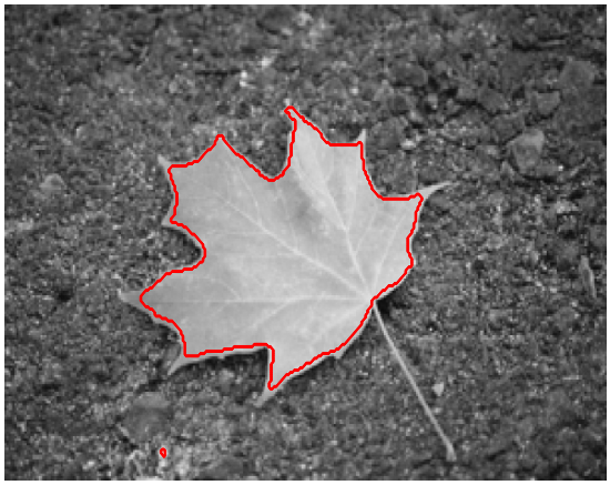
When the IIH image is added as a channel to the grayscale image, we smooth each channel and then apply $K$ -means clustering for the SaT methods. For the other segmentation methods, we consider their multichannel extensions to process the two channels that are composed of grayscale and IIH.

For the images in Figure 5 (after rescaling the pixel intensities to $[0,1]$ ), we corrupt them with motion blur fspecial(‘motion’, 5,0) followed by Gaussian noise with mean 0 and variance 0.001. We tune the parameters $\lambda\in[0.25,5]$ and $\mu\in[5,60]$ for the SaT methods. For each image, the ground truth is determined from the segmentation results by three human subjects. A pixel is declared an object of interest in the ground truth if at least two subjects agree AlpertGBB07. The DICE indices and computational times of the segmentation algorithms are recorded in Table 3 while the segmentation results and their ground truths are presented in Figures 8-14. Note that some segmentation results have the image border segmented because of the boundary artifacts created by the IIH image (see Figures 6(b) and 6(e)). For all four images, AITV SaT (ADMM) is among the top three methods with the highest DICE indices. It provides satisfactory results in about two seconds. Moreover, it outperforms its DCA counterpart in terms of DICE indices and computational times, especially for Figure 5(b). For Figures 8-12, although both algorithms solve the same model (7), they output different results. As (7) is nonconvex, it is possible that ADMM and DCA attain different solutions.

4.3 Real Color Images

Four real color images taken from martin-2001 are presented in Figure for segmentation. The images are corrupted with either Gaussian noise of mean zero and variance 0.025 or 10% SP noise. We segment Figure with $k=3$ regions, Figure with $k=5$ regions, Figure with $k=6$ regions, and Figure with $k=8$ regions. Because ground truth is unavailable, we use PSNR to evaluate the segmentation result as a piecewise-constant approximation of the original image. For the SLaT methods, we tune the parameters $\lambda\in[2,30]$ and $\mu\in[0.05,1.0]$ for all the images.

Table records the PSNR values and computational times in seconds of the segmentation algorithms while Figures - present the visual results. Overall, AITV SLaT (ADMM) is generally among the top three methods with the best PSNR values for both noise cases. In fact, for SP noise, AITV SLaT (ADMM) has the second best PSNRs while being significantly faster than TV^p MS that has the best PSNRs.

In Figure , the sand lines are segmented in fine details by the SLaT methods, ICTM, and TV^p MS in the Gaussian noise case and by the (original) SLaT, AITV SLaT, and TV^p MS in the SP noise case. In Figure , TV^p SLaT, AITV SLAT, AITV FR, TV^p MS, and SaT-Potts can clearly segment the multiple rows of windows on the top part of the building on the right. Under the SP noise, no algorithms succeed in the windows, but AITV SLaT (ADMM) and TV^p MS are able to preserve some parts of the man’s eyes and the palm trees’ green color and foliage. Despite AITV SLaT (ADMM) having a lower PSNR, the palm trees are greener in the segmentation result of AITV SLaT (ADMM) than TV^p MS. In Figure , under Gaussian noise, despite having lower PSNRs, both ADMM and DCA of AITV SLaT are able to more clearly segment the bottom half of the wheel at the lower right corner than TV^p SLaT and TV^p MS. Moreover, the roofs in the segmentation results of AITV SLaT are mostly brown while they have a considerable amount of green in the results of the TV^p models. Under the SP noise, AITV SLaT (ADMM) provides the most visually appealing segmentation result even though its PSNR is not the best. TV^p MS identifies the green color of the grass and most of the wheels on the bottom right corner compared to any other methods. Lastly, for Figure , under Gaussian noise, the SLaT methods, the Potts methods, and TV^p MS produce visually similar segmentation results. Under SP noise, AITV SLaT (ADMM) and TV^p MS segment more windows at the top of the building than any other methods. For all four figures, AITV SLaT (ADMM) and AITV SLaT (DCA) produce segmentation results with similar PSNR values, but the former is up to five times faster than the latter. Although ICTM and SaT-Potts are the fastest methods, their segmentation results are less satisfactory.

4.3.1 HSV vs. Lab

The HSV (hue, saturation, and value) space is another popular, approximately uniform color space that could be used instead of Lab space for the SLaT methods. It was used to derived features for improving image segmentation algorithms benninghoff2014efficient; burdescu2009new; chen2008fast; huang2007segmentation; paschos2001perceptually; sural2002segmentation. Some works paschos2001perceptually; toure2018best claim that HSV space is better than Lab space for image segmentation. However, we provide numerical evidence to show that HSV space may not be as effective as Lab space for the SLaT methods.

To compare the segmentation results between HSV and Lab for the AITV SLaT method, we replace Lab with HSV in Algorithm 1 and apply the HSV-based algorithm to the images in Figure corrupted with Gaussian noise with mean zero and variance 0.025. Figure compares the segmentation results and the PSNR values between using HSV and Lab spaces. Overall, we observe that using Lab space for AITV SLaT leads to higher PSNR values and more detailed segmentation. For Figure , using Lab space identifies more of the fine sand lines than HSV space. Unlike using HSV space, AITV SLaT with Lab is able to identify the windows on the right side of Figure and the wheel on the bottom right corner of Figure . Lastly, for Figure , the tulips are clearly redder and more segmented in the result of AITV SLaT with Lab than with HSV.

4.4 Parameter Analysis

(a) Changes in PSNR with respect to

\lambda

with

\mu=0.10

fixed.

(b) Changes in PSNR with respect to

\mu

with

\lambda=10

fixed.

Figure 15: Sensitivity analysis on the model parameters

\lambda

and

\mu

to Figure corrupted by Gaussian noise with mean 0 and variance 0.025.

(a) Changes in PSNR with respect to

\delta_{0}

with

\sigma=1.25

fixed.

(b) Changes in computational time with respect to

\delta_{0}

with

\sigma=1.25

fixed.

\sigma

with

\delta_{0}=2

fixed.

(d) Changes in computational time with respect to

\sigma

with

\delta_{0}=2

fixed.

Figure 16: Sensitivity analysis on the ADMM algorithm parameters

\delta_{0}

and

\sigma

4.4.1 Model Parameters of (7)

We analyze the following parameters in (7):

•

$\lambda$ : this fidelity parameter weighs how close the approximation $Au^{*}$ is to the original image $f$ , where $u^{*}$ is a solution to (7). When the image $f$ has a large amount of noise, choosing a small value for $\lambda$ is recommended.
•

$\mu$ : this smoothing parameter determines the smoothness of the solution $u^{*}$ of (7), which may help with denoising. However, choosing a large value for $\mu$ will deteriorate important edge information in $u^{*}$ .
•

$\alpha\in[0,1]$ : this sparsity parameter determines the gradient vector sparsity at each pixel, which is important in preserving edge information. However, choosing a large $\alpha$ may result in preserving some noise in the solution $u^{*}$ .

To perform sensitivity analysis on the model parameters, we apply AITV SLaT (ADMM) with parameters $\delta_{0}=2$ and $\sigma=1.25$ to Figure corrupted with Gaussian noise with mean 0 and variance 0.025. We examine the sparsity parameter $\alpha\in\{0.2,0.3,\ldots,0.8\}$ while we vary either the fidelity parameter $\lambda$ with $\mu=0.10$ fixed or the smoothing parameter $\mu$ with $\lambda=10$ fixed. The sensitivity analysis is visualized in Figure 15.

Figure 15(a) shows that the PSNR has a concave relationship with respect to the fidelity parameter $\lambda$ for each value of $\alpha$ . We observe that larger value of $\alpha$ leads to higher PSNR for smaller value of $\lambda$ . More specifically, when $\lambda\leq 5.0$ , the order of the PSNR curves follows the increasing value of $\alpha$ . However, the order is reversed when $\lambda$ becomes large enough, such as when $\lambda\geq 10$ . Figure 15(b) shows that with respect to the smoothing parameter, PSNR is generally increasing when $0.4\leq\alpha\leq 0.8$ while it appears to be robust for $\alpha=0.2,0.3$ .

4.4.2 Algorithm Parameters of Algorithm 2

We analyze the following parameters introduced in the ADMM algorithm that solves (7):

•

$\delta_{0}$ : this penalty parameter weighs the quadratic difference between the original variable $\nabla u$ and the auxiliary variable $w$ .
•

$\sigma$ : this penalty multiplier determines the numerical convergence speed of the ADMM algorithm.

We perform sensitivity analysis on AITV SLaT (ADMM) with model parameters $\lambda=10,\mu=0.1$ , and $\alpha=0.2$ to Figure corrupted with Gaussian noise with mean 0 and variance 0.025. When varying $\delta_{0}$ , we fix $\sigma=1.25$ while when varying $\sigma$ , we fix $\delta_{0}=2$ . Figure 16 visualizes the sensitivity analysis of the algorithm parameters.

According to Figures 16(a)-16(b), the penalty parameter $\delta_{0}$ does not have much influence on the PSNR, but it does affect the speed of the ADMM algorithm. When $\delta_{0}<1.5$ , the computational time is between 9.5 to 15.5 seconds, but when $\delta_{0}\geq 1.5$ , it decreases to between about 9 to 12 seconds. As shown in Figures 16(c)-16(d), the penalty multiplier $\sigma$ does have an impact on both the PSNR and the algorithm’s numerical convergence. As $\sigma$ increases, the PSNR generally decreases. When $\sigma<1.25$ , the algorithm can be as slow as up to 22 seconds, but when $\sigma\geq 1.25$ , it does speed up to between 8 and 13 seconds.

5 Conclusion

In this paper, we proposed an efficient ADMM algorithm for the SaT/SLaT framework that utilizes AITV regularization. When designing the ADMM algorithm, we incorporated the proximal operator for the $\ell_{1}-\alpha\ell_{2}$ regularization louY18. We provided convergence analysis of ADMM to demonstrate that the algorithm subsequentially converges to an KKT point under certain conditions. In our numerical experiments, the AITV SaT/SLaT using our ADMM algorithm produces high-quality segmentation results within a few seconds. In addition, this work shows the effectiveness of using nonconvex regularizations in image processing. As for future works, we will explore other nonconvex regularizations, such as transformed $\ell_{1}$ zhang2014minimization; zhang2018minimization, as alternative options to AITV and TV ${}^{p}(0<p<1)$ under the SaT/SLaT framework. To simplify the SLaT framework for color images, we plan to apply these nonconvex regularizations in quaternion space to complement the quaternion-based SaT model wu2022efficient with $\ell_{1}/\ell_{2}$ regularization rahimi2019scale; wang2019accelerated; wang2021limited; wang2021minimizing.

Acknowledgments

The authors thank Xu Li for providing code and answering questions about the IIH image in li2020three. The authors also thank Elisha Dayag for writing the initial code for the TV^p-regularized Mumford-Shah model described in li2020tv. The work was partially supported by NSF grants DMS-1854434, DMS-1952644, DMS-2151235, DMS-2219904, and CAREER 1846690. We thank the two reviewers for their valuable feedback in improving the quality of the manuscript.

Declarations

Conflict of Interest The authors declare that they have no known competing financial interests or personal relationships that could have appeared to influence the work reported in this paper.

Availability of Data and Material The images in Section 4.1 are available from the corresponding author on reasonable request. The images in Section 4.2 are available at https://www.wisdom.weizmann.ac.il/~vision/Seg_Evaluation_DB/. The images in Section 4.3 are available at https://www2.eecs.berkeley.edu/Research/Projects/CS/vision/bsds/.

Code Availability Code generated is available at https://github.com/kbui1993/Official_AITV_SaT_SLaT.

Appendix A Proofs of Section 3.3

A.1 Proof of Lemma 3.3

Proof.

It is straightforward that $u^{\top}A^{\top}Au=\|Au\|_{2}^{2}\geq 0$ and $u^{\top}\nabla^{\top}\nabla u=\|\nabla u\|_{2}^{2}\geq 0$ for any $u\in X$ , so $\zeta\geq 0$ . If $\zeta=0,$ then there exists a nonzero vector $x\in X$ such that $\lambda\|Ax\|_{2}^{2}+(\mu+\delta_{0})\|\nabla x\|_{2}^{2}=\lambda x^{\top}A^{\top}Ax+(\mu+\delta_{0})x^{\top}\nabla^{\top}\nabla x=0.$ Then we shall have $x\in\text{ker}(A)\cap\text{ker}(\nabla)$ , contradicting that $\text{ker}(A)\cap\text{ker}(\nabla)=\{0\}$ . Therefore, $\zeta>0$ and hence we get

\displaystyle\lambda\|Au\|_{2}^{2}+(\mu+\delta_{0})\|\nabla u\|_{2}^{2}\geq\zeta\|u\|_{2}^{2}\hskip 9.24994pt\forall u\in X.

As $\delta_{t+1}\geq\delta_{t}$ ( $\sigma\geq 1$ ), $\mathcal{L}_{\delta_{t}}(u,w_{t},z_{t})$ is a strongly convex function of $u$ with parameter $\zeta>0$ . Fixing $w_{t},z_{t}$ , the minimizer $u_{t+1}$ of $\mathcal{L}_{\delta_{t}}(u,w_{t},z_{t})$ in (10a) satisfies the following inequality (beck2017first, Theorem 5.25),

\displaystyle\begin{split}&\mathcal{L}_{\delta_{t}}(u_{t+1},w_{t},z_{t})-\mathcal{L}_{\delta_{t}}(u_{t},w_{t},z_{t})\leq-\frac{\zeta}{2}\|u_{t+1}-u_{t}\|_{2}^{2}.\end{split}

(18)

As $w_{t+1}$ is the optimal solution to (10b), we have

\displaystyle\mathcal{L}_{\delta_{t}}(u_{t+1},w_{t+1},z_{t})-\mathcal{L}_{\delta_{t}}(u_{t+1},w_{t},z_{t})\leq 0.

(19)

It follows from the update (10c) that

\displaystyle\begin{aligned} \mathcal{L}_{\delta_{t}}(u_{t+1},w_{t+1},z_{t+1})-\mathcal{L}_{\delta_{t}}(u_{t+1},w_{t+1},z_{t})&=\langle z_{t+1}-z_{t},\nabla u_{t+1}-w_{t+1}\rangle\\ &=\frac{1}{\delta_{t}}\|z_{t+1}-z_{t}\|_{2}^{2}.\end{aligned}

(20)

Similarly, we get

\displaystyle\begin{aligned} \mathcal{L}_{\delta_{t+1}}(u_{t+1},w_{t+1},z_{t+1})-\mathcal{L}_{\delta_{t}}(u_{t+1},w_{t+1},z_{t+1})=&\frac{\delta_{t+1}-\delta_{t}}{2}\|\nabla u_{t+1}-w_{t+1}\|_{2}^{2}\\ =&\frac{\delta_{t+1}-\delta_{t}}{2\delta_{t}^{2}}\|z_{t+1}-z_{t}\|_{2}^{2}.\end{aligned}

(21)

Combining (18)-(21) leads to the desired inequality

	$\displaystyle\mathcal{L}_{\delta_{t+1}}(u_{t+1},w_{t+1},z_{t+1})-\mathcal{L}_{\delta_{t}}(u_{t},w_{t},z_{t})$	$\displaystyle\leq\frac{\delta_{t+1}-\delta_{t}}{2\delta_{t}^{2}}\\|z_{t+1}-z_{t}\\|_{2}^{2}+\frac{1}{\delta_{t}}\\|z_{t+1}-z_{t}\\|_{2}^{2}$
		$\displaystyle\hskip 9.24994pt-\frac{\zeta}{2}\\|u_{t+1}-u_{t}\\|_{2}^{2}$
		$\displaystyle=\frac{\sigma+1}{2\sigma^{t}\delta_{0}}\\|z_{t+1}-z_{t}\\|_{2}^{2}-\frac{\zeta}{2}\\|u_{t+1}-u_{t}\\|_{2}^{2}.$

∎

A.2 Proof of Proposition 3.1

Proof.

(a) We start by proving the boundedness of $\{z_{t}\}_{t=1}^{\infty}.$ The optimality condition of (10b) at iteration $t$ is expressed by

\displaystyle\begin{split}0&\in\partial\left(\|w_{t+1}\|_{1}-\alpha\|w_{t+1}\|_{2,1}\right)-\delta_{t}\left(\nabla u_{t+1}-w_{t+1}\right)-z_{t}.\end{split}

(22)

Together with (10c), we have

\displaystyle\begin{split}z_{t+1}&\in\partial\left(\|w_{t+1}\|_{1}-\alpha\|w_{t+1}\|_{2,1}\right)\subset\partial\|w_{t+1}\|_{1}-\alpha\partial\|w_{t+1}\|_{2,1},\end{split}

(23)

which implies that there exist two vectors $v_{1}\in\partial\|w_{t+1}\|_{1}$ and $v_{2}\in\partial\|w_{t+1}\|_{2,1}$ such that $z_{t+1}=v_{1}-\alpha v_{2}$ . For any $v\in\partial\|w\|_{1}$ , we have

\displaystyle(v_{x})_{i,j}=\sign((w_{x})_{i,j})\text{ and }(v_{y})_{i,j}=\sign((w_{y})_{i,j}),

(24)

which guarantees that $\|v\|_{\infty}\leq 1.$ If $z\in\partial\|w\|_{2,1}$ , then

\displaystyle z_{i,j}=\begin{cases}\displaystyle\frac{w_{i,j}}{\|w_{i,j}\|_{2}}&\text{ if }\|w_{i,j}\|_{2}\neq 0,\\ \in\{z_{i,j}\in\mathbb{R}^{2}:\|z_{i,j}\|_{2}\leq 1\}&\text{ if }\|w_{i,j}\|_{2}=0.\end{cases}

(25)

By (25), we have $\|(v_{2})_{i,j}\|_{2}\leq 1$ , which means that $\|v_{2}\|_{\infty}\leq 1$ . As a result, $\|z_{t+1}\|_{\infty}\leq\|v_{1}\|_{\infty}+\alpha\|v_{2}\|_{\infty}\leq 2$ . Altogether, we arrive at an upper bound, i.e.,

\displaystyle\begin{split}\|z_{t+1}\|_{2}&=\sqrt{\sum_{i,j}\left(|(z_{t+1,x})_{i,j}|^{2}+|(z_{t+1,y})_{i,j}|^{2}\right)}\\ &\leq\sqrt{2^{2}(2MN)}=2\sqrt{2MN}.\end{split}

(26)

By telescoping summation of (13), we have for all $t$ that

	$\displaystyle\mathcal{L}_{\delta_{t+1}}(u_{t+1},w_{t+1},z_{t+1})\leq$	$\displaystyle\mathcal{L}_{\delta_{0}}(u_{0},w_{0},z_{0})+\frac{(\sigma+1)}{2\delta_{0}}\sum_{i=0}^{t}\frac{1}{\sigma^{i}}\\|z_{i+1}-z_{i}\\|_{2}^{2}$
	$\displaystyle\leq$	$\displaystyle\mathcal{L}_{\delta_{0}}(u_{0},w_{0},z_{0})+\frac{(\sigma+1)}{2\delta_{0}}\sum_{i=0}^{\infty}\frac{1}{\sigma^{i}}\\|z_{i+1}-z_{i}\\|_{2}^{2}.$

Now that $\{z_{t}\}_{t=1}^{\infty}$ is bounded, then $\{\|z_{t+1}-z_{t}\|_{2}^{2}\}_{t=1}^{\infty}$ is bounded. Denote $C:=\displaystyle\sup_{t\in\mathbb{N}}\|z_{t+1}-z_{t}\|_{2}^{2}$ . If $\sigma=1$ and $\displaystyle\sum_{i=0}^{\infty}\|z_{i+1}-z_{i}\|_{2}^{2}<\infty$ , then $\{\mathcal{L}_{\delta_{t}}(u_{t},w_{t},z_{t})\}_{t=1}^{\infty}$ is uniformly bounded above. On the other hand, if $\sigma>1$ , then we get

\displaystyle\mathcal{L}_{\delta_{t+1}}(u_{t+1},w_{t+1},z_{t+1})\leq\mathcal{L}_{\delta_{0}}(u_{0},w_{0},z_{0})+\frac{C(\sigma+1)}{2\delta_{0}}\sum_{i=0}^{\infty}\frac{1}{\sigma^{i}}<\infty,

where the infinite sum converges for $\sigma>1$ . In either case, we have that $\{\mathcal{L}_{\delta_{t}}(u_{t},w_{t},z_{t})\}_{t=1}^{\infty}$ is uniformly bounded above, and hence there exists a constant $\tilde{C}>0$ such that $\mathcal{L}_{\delta_{t}}(u_{t},w_{t},z_{t})<\tilde{C}$ .

Since $\|w\|_{2,1}\leq\|w\|_{1}$ , we have

\displaystyle\frac{\mu}{2}\|\nabla u_{t}\|_{2}^{2}-\frac{1}{2\delta_{t}}\|z_{t}\|_{2}^{2}\leq\mathcal{L}_{\delta_{t}}(u_{t},w_{t},z_{t})\leq\tilde{C}.

This suggests an upper bound of $\|\nabla u_{t}\|_{2},$ i.e.,

\displaystyle\|\nabla u_{t}\|_{2}\leq\sqrt{\frac{2}{\mu}\left(\tilde{C}+\frac{1}{2\delta_{t}}\|z_{t}\|_{2}^{2}\right)}\leq\sqrt{\frac{2}{\mu}\left(\tilde{C}+\frac{4MN}{\delta_{0}}\right)}.

Moreover, we observe that

\displaystyle\frac{\lambda}{2}\|f-Au_{t}\|_{2}^{2}-\frac{1}{2\delta_{t}}\|z_{t}\|_{2}^{2}\leq\mathcal{L}_{\delta_{t}}(u_{t},w_{t},z_{t})\leq\tilde{C}.

As $\{z_{t}\}_{t=1}^{\infty}$ is bounded, then $\{\|f-Au_{t}\|_{2}^{2}\}_{t=1}^{\infty}$ is bounded as well. Altogether $\{F(u_{t})\}_{t=1}^{\infty}$ is a bounded sequence, and hence we conclude that $\{u_{t}\}_{t=1}^{\infty}$ is bounded by coercivity in Lemma 3.1. Lastly, from (10c), we have

\displaystyle\|w_{t}\|_{2}\leq\left\|\nabla u_{t}-\frac{z_{t}-z_{t-1}}{\delta_{t-1}}\right\|_{2}^{2}\leq\frac{4\sqrt{2MN}}{\delta_{0}}+\sqrt{\frac{2}{\mu}\left(\tilde{C}+\frac{4MN}{\delta_{0}}\right)},

proving that $\{w_{t}\}_{t=1}^{\infty}$ is bounded.

(b) By Lemma 3.3, we can derive

	$\displaystyle\mathcal{L}_{\delta_{t+1}}(u_{t+1},w_{t+1},z_{t+1})\leq$	$\displaystyle\mathcal{L}_{0}(u_{0},w_{0},z_{0})+\frac{(\sigma+1)}{2\delta_{0}}\sum_{i=0}^{t}\frac{1}{\sigma^{i}}\\|z_{i+1}-z_{i}\\|_{2}^{2}$
		$\displaystyle-\frac{\zeta}{2}\sum_{i=0}^{t}\\|u_{i+1}-u_{i}\\|_{2}^{2}.$

By (26), we have

\displaystyle\begin{split}\mathcal{L}_{\delta_{t+1}}(u_{t+1},w_{t+1},z_{t+1})&\geq-\frac{1}{2\delta_{t+1}}\|z_{t+1}\|_{2}^{2}\geq-\frac{4MN}{\delta_{0}},\;\forall t\in\mathbb{N}.\end{split}

(27)

Combining the two inequalities gives us

	$\displaystyle-\frac{4MN}{\delta_{0}}+\frac{\zeta}{2}\sum_{i=0}^{t}\\|u_{i+1}-u_{i}\\|_{2}^{2}\leq$	$\displaystyle\mathcal{L}_{\delta_{t+1}}(u_{t+1},w_{t+1},z_{t+1})+\frac{\zeta}{2}\sum_{i=0}^{t}\\|u_{i+1}-u_{i}\\|_{2}^{2}$
	$\displaystyle\leq$	$\displaystyle\mathcal{L}_{0}(u_{0},w_{0},z_{0})+\frac{(\sigma+1)}{2\delta_{0}}\sum_{i=0}^{t}\frac{1}{\sigma^{i}}\\|z_{i+1}-z_{i}\\|_{2}^{2}.$

As $t\rightarrow\infty$ , we obtain

\displaystyle 0

\displaystyle\leq\frac{\zeta}{2}\sum_{i=0}^{\infty}\|u_{i+1}-u_{i}\|_{2}^{2}\leq\mathcal{L}_{\delta_{0}}(u_{0},w_{0},z_{0})+\frac{(\sigma+1)}{2\delta_{0}}\sum_{i=0}^{\infty}\frac{1}{\sigma^{i}}\|z_{i+1}-z_{i}\|_{2}^{2}+\frac{4MN}{\delta_{0}}.

Earlier in proving the boundedness of $\{\mathcal{L}_{\delta_{t}}(u_{t},w_{t},z_{t})\}_{t=1}^{\infty}$ , we show that the summation $\displaystyle\sum_{i=0}^{\infty}\frac{1}{\sigma^{i}}\|z_{i+1}-z_{i}\|_{2}^{2}$ converges. As a result, the summation $\displaystyle\sum_{i=0}^{\infty}\|u_{i+1}-u_{i}\|_{2}^{2}$ converges, which implies that $u_{t+1}-u_{t}\rightarrow 0$ . ∎

References

(1) Sharon Alpert, Meirav Galun, Ronen Basri, and Achi Brandt. Image segmentation by probabilistic bottom-up aggregation and cue integration. In Proceedings of the IEEE Conference on Computer Vision and Pattern Recognition, June 2007.
(2) Luigi Ambrosio and Vincenzo Maria Tortorelli. Approximation of functional depending on jumps by elliptic functional via t-convergence. Communications on Pure and Applied Mathematics, 43(8):999–1036, 1990.
(3) David Arthur and Sergei Vassilvitskii. K-means++: the advantages of careful seeding. In 2007 ACM-SIAM Symposium on Discrete Algorithms (SODA’07), pages 1027–1035, 2007.
(4) Leah Bar, Tony F Chan, Ginmo Chung, Miyoun Jung, Nahum Kiryati, Rami Mohieddine, Nir Sochen, and Luminita A Vese. Mumford and Shah model and its applications to image segmentation and image restoration. In Handbook of Mathematical Methods in Imaging. Springer, 2011.
(5) Amir Beck. First-order methods in optimization. SIAM, Philadelphia, 2017.
(6) Heike Benninghoff and Harald Garcke. Efficient image segmentation and restoration using parametric curve evolution with junctions and topology changes. SIAM Journal on Imaging Sciences, 7(3):1451–1483, 2014.
(7) Harald Birkholz. A unifying approach to isotropic and anisotropic total variation denoising models. Journal of computational and applied mathematics, 235(8):2502–2514, 2011.
(8) Stephen Boyd, Neal Parikh, Eric Chu, Borja Peleato, Jonathan Eckstein, et al. Distributed optimization and statistical learning via the alternating direction method of multipliers. Foundations and Trends® in Machine learning, 3(1):1–122, 2011.
(9) Kevin Bui, Fredrick Park, Yifei Lou, and Jack Xin. A weighted difference of anisotropic and isotropic total variation for relaxed Mumford-Shah color and multiphase image segmentation. SIAM Journal on Imaging Sciences, 14(3):1078–1113, 2021.
(10) Dumitru Dan Burdescu, Marius Brezovan, Eugen Ganea, and Liana Stanescu. A new method for segmentation of images represented in a hsv color space. In Advanced Concepts for Intelligent Vision Systems: 11th International Conference, ACIVS 2009, Bordeaux, France, September 28–October 2, 2009. Proceedings 11, pages 606–617. Springer, 2009.
(11) Xiaohao Cai, Raymond Chan, Mila Nikolova, and Tieyong Zeng. A three-stage approach for segmenting degraded color images: Smoothing, lifting and thresholding (SLaT). Journal of Scientific Computing, 72(3):1313–1332, 2017.
(12) Xiaohao Cai, Raymond Chan, and Tieyong Zeng. A two-stage image segmentation method using a convex variant of the Mumford–Shah model and thresholding. SIAM Journal on Imaging Sciences, 6(1):368–390, 2013.
(13) Wenfei Cao, Jian Sun, and Zongben Xu. Fast image deconvolution using closed-form thresholding formulas of $L_{q}(q=\frac{1}{2},\frac{2}{3})$ regularization. Journal of Visual Communication and Image Representation, 24(1):31–41, 2013.
(14) Antonin Chambolle. Finite-differences discretizations of the Mumford-Shah functional. ESAIM: Mathematical Modelling and Numerical Analysis, 33(2):261–288, 1999.
(15) Antonin Chambolle and Gianni Dal Maso. Discrete approximation of the Mumford-Shah functional in dimension two. ESAIM: Mathematical Modelling and Numerical Analysis, 33(4):651–672, 1999.
(16) Antonin Chambolle and Thomas Pock. A first-order primal-dual algorithm for convex problems with applications to imaging. Journal of Mathematical Imaging and Vision, 40(1):120–145, 2011.
(17) Raymond Chan, Hongfei Yang, and Tieyong Zeng. A two-stage image segmentation method for blurry images with poisson or multiplicative gamma noise. SIAM Journal on Imaging Sciences, 7(1):98–127, 2014.
(18) Raymond H Chan and Michael K Ng. Conjugate gradient methods for Toeplitz systems. SIAM Review, 38(3):427–482, 1996.
(19) Tony F Chan, Selim Esedoglu, and Mila Nikolova. Algorithms for finding global minimizers of image segmentation and denoising models. SIAM Journal on Applied Mathematics, 66(5):1632–1648, 2006.
(20) Tony F Chan, B Yezrielev Sandberg, and Luminita A Vese. Active contours without edges for vector-valued images. Journal of Visual Communication and Image Representation, 11(2):130–141, 2000.
(21) Tony F Chan and Luminita A Vese. Active contours without edges. IEEE Transactions on Image Processing, 10(2):266–277, 2001.
(22) Huibin Chang, Yifei Lou, Yuping Duan, and Stefano Marchesini. Total variation–based phase retrieval for poisson noise removal. SIAM Journal on Imaging Sciences, 11(1):24–55, 2018.
(23) Huibin Chang, Yifei Lou, Michael K Ng, and Tieyong Zeng. Phase retrieval from incomplete magnitude information via total variation regularization. SIAM Journal on Scientific Computing, 38(6):A3672–A3695, 2016.
(24) Rick Chartrand and Wotao Yin. Iteratively reweighted algorithms for compressive sensing. In 2008 IEEE International Conference on Acoustics, Speech and Signal Processing, pages 3869–3872. IEEE, 2008.
(25) Tse-Wei Chen, Yi-Ling Chen, and Shao-Yi Chien. Fast image segmentation based on K-means clustering with histograms in HSV color space. In 2008 IEEE 10th workshop on multimedia signal processing, pages 322–325. IEEE, 2008.
(26) X Chen, MK Ng, and C Zhang. Non-lipshitz $\ell_{p}$ -regularization and box constrained model for image reconstruction. IEEE Transactions on Image Processing, 21(12):4709–4721, 2012.
(27) Francis Clarke. Functional analysis, calculus of variations and optimal control, volume 264. Springer Science & Business Media, Heidelberg, 2013.
(28) Laurent Condat. Discrete total variation: New definition and minimization. SIAM Journal on Imaging Sciences, 10(3):1258–1290, 2017.
(29) Wei Deng and Wotao Yin. On the global and linear convergence of the generalized alternating direction method of multipliers. Journal of Scientific Computing, 66(3):889–916, 2016.
(30) Lee R Dice. Measures of the amount of ecologic association between species. Ecology, 26(3):297–302, 1945.
(31) Liang Ding and Weimin Han. $\alpha\ell_{1}-\beta\ell_{2}$ regularization for sparse recovery. Inverse Problems, 35(12):125009, 2019.
(32) Selim Esedoglu and Yen-Hsi Richard Tsai. Threshold dynamics for the piecewise constant Mumford–Shah functional. Journal of Computational Physics, 211(1):367–384, 2006.
(33) Ernie Esser, Xiaoqun Zhang, and Tony F Chan. A general framework for a class of first order primal-dual algorithms for convex optimization in imaging science. SIAM Journal on Imaging Sciences, 3(4):1015–1046, 2010.
(34) Huanmin Ge, Wengu Chen, and Michael K Ng. New restricted isometry property analysis for $\ell_{1}-\ell_{2}$ minimization methods. SIAM Journal on Imaging Sciences, 14(2):530–557, 2021.
(35) Pascal Getreuer. Chan–Vese segmentation. Image Processing On Line, 2:214–224, 2012.
(36) Massimo Gobbino. Finite difference approximation of the Mumford-Shah functional. Communications on Pure and Applied Mathematics: A Journal Issued by the Courant Institute of Mathematical Sciences, 51(2):197–228, 1998.
(37) Tom Goldstein, Xavier Bresson, and Stanley Osher. Geometric applications of the split Bregman method: segmentation and surface reconstruction. Journal of Scientific Computing, 45(1-3):272–293, 2010.
(38) Tom Goldstein and Stanley Osher. The split Bregman method for L1-regularized problems. SIAM Journal on Imaging Sciences, 2(2):323–343, 2009.
(39) Shuhang Gu, Qi Xie, Deyu Meng, Wangmeng Zuo, Xiangchu Feng, and Lei Zhang. Weighted nuclear norm minimization and its applications to low level vision. International Journal of Computer Vision, 121(2):183–208, 2017.
(40) Deren Han, Defeng Sun, and Liwei Zhang. Linear rate convergence of the alternating direction method of multipliers for convex composite programming. Mathematics of Operations Research, 43(2):622–637, 2018.
(41) John A Hartigan and Manchek A Wong. A K-means clustering algorithm. Journal of the Royal Statistical Society: Series C (Applied Statistics), 28(1):100–108, 1979.
(42) Michael Hintermüller and Tao Wu. Nonconvex $\text{TV}^{q}$ -models in image restoration: Analysis and a trust-region regularization–based superlinearly convergent solver. SIAM Journal on Imaging Sciences, 6(3):1385–1415, 2013.
(43) Zujun Hou. A review on MR image intensity inhomogeneity correction. International Journal of Biomedical Imaging, 2006, 2006.
(44) Zhi-Kai Huang and De-Hui Liu. Segmentation of color image using em algorithm in hsv color space. In 2007 International Conference on Information Acquisition, pages 316–319. IEEE, 2007.
(45) Miyoun Jung. Piecewise-smooth image segmentation models with $L^{1}$ data-fidelity terms. Journal of Scientific Computing, 70(3):1229–1261, 2017.
(46) Miyoun Jung, Myeongmin Kang, and Myungjoo Kang. Variational image segmentation models involving non-smooth data-fidelity terms. Journal of Scientific Computing, 59(2):277–308, 2014.
(47) Alessandro Lanza, Serena Morigi, and Fiorella Sgallari. Constrained $\text{TV}_{p}-\ell_{2}$ model for image restoration. Journal of Scientific Computing, 68(1):64–91, 2016.
(48) Hoai An Le Thi and Tao Pham Dinh. DC programming and DCA: thirty years of developments. Mathematical Programming, 169(1):5–68, 2018.
(49) Chunming Li, Chiu-Yen Kao, John C Gore, and Zhaohua Ding. Minimization of region-scalable fitting energy for image segmentation. IEEE Transactions on Image Processing, 17(10):1940–1949, 2008.
(50) Fang Li, Michael K Ng, Tie Yong Zeng, and Chunli Shen. A multiphase image segmentation method based on fuzzy region competition. SIAM Journal on Imaging Sciences, 3(3):277–299, 2010.
(51) Fang Li, Stanley Osher, Jing Qin, and Ming Yan. A multiphase image segmentation based on fuzzy membership functions and L1-norm fidelity. Journal of Scientific Computing, 69(1):82–106, 2016.
(52) Fang Li and Yuanming Zhu. Smoothing and clustering guided image decolorization. Image Analysis and Stereology, 40(1), 2021.
(53) Peng Li, Wengu Chen, Huanmin Ge, and Michael K Ng. $\ell_{1}-\alpha\ell_{2}$ minimization methods for signal and image reconstruction with impulsive noise removal. Inverse Problems, 36(5):055009, 2020.
(54) Xu Li, Xiaoping Yang, and Tieyong Zeng. A three-stage variational image segmentation framework incorporating intensity inhomogeneity information. SIAM Journal on Imaging Sciences, 13(3):1692–1715, 2020.
(55) Yutong Li, Chunlin Wu, and Yuping Duan. The $\text{TV}_{p}$ regularized Mumford-Shah model for image labeling and segmentation. IEEE Transactions on Image Processing, 29:7061–7075, 2020.
(56) Yifei Lou, Stanley Osher, and Jack Xin. Computational aspects of constrained $L_{1}-L_{2}$ minimization for compressive sensing. In Modelling, Computation and Optimization in Information Systems and Management Sciences, pages 169–180. Springer, 2015.
(57) Yifei Lou and Ming Yan. Fast L1-L2 minimization via a proximal operator. Journal of Scientific Computing, 74(2):767–785, 2018.
(58) Yifei Lou, Penghang Yin, Qi He, and Jack Xin. Computing sparse representation in a highly coherent dictionary based on difference of $L_{1}$ and $L_{2}$ . Journal of Scientific Computing, 64(1):178–196, 2015.
(59) Yifei Lou, Tieyong Zeng, Stanley Osher, and Jack Xin. A weighted difference of anisotropic and isotropic total variation model for image processing. SIAM Journal on Imaging Sciences, 8(3):1798–1823, 2015.
(60) Quang-Tuan Luong. Color in computer vision. In Handbook of Pattern Recognition and Computer Vision, pages 311–368. World Scientific, 1993.
(61) David Martin, Charless Fowlkes, Doron Tal, and Jitendra Malik. A database of human segmented natural images and its application to evaluating segmentation algorithms and measuring ecological statistics. In Computer Vision, 2001. ICCV 2001. Proceedings. Eighth IEEE International Conference on, volume 2, pages 416–423. IEEE, 2001.
(62) Barry Merriman, James K Bence, and Stanley J Osher. Motion of multiple junctions: A level set approach. Journal of Computational Physics, 112(2):334–363, 1994.
(63) David Mumford and Jayant Shah. Optimal approximations by piecewise smooth functions and associated variational problems. Communications on Pure and Applied Mathematics, 42(5):577–685, 1989.
(64) Michael K Ng, Raymond H Chan, and Wun-Cheung Tang. A fast algorithm for deblurring models with Neumann boundary conditions. SIAM Journal on Scientific Computing, 21(3):851–866, 1999.
(65) Shunsuke Ono. ${L}_{0}$ gradient projection. IEEE Transactions on Image Processing, 26(4):1554–1564, 2017.
(66) George Paschos. Perceptually uniform color spaces for color texture analysis: an empirical evaluation. IEEE transactions on Image Processing, 10(6):932–937, 2001.
(67) Tao Pham Dinh and Hoai An Le Thi. Convex analysis approach to DC programming: Theory, algorithms and applications. Acta Mathematica Vietnamica, 22(1):289–355, 1997.
(68) Tao Pham Dinh and Hoai An Le Thi. A DC optimization algorithm for solving the trust-region subproblem. SIAM Journal on Optimization, 8(2):476–505, 1998.
(69) Thomas Pock, Antonin Chambolle, Daniel Cremers, and Horst Bischof. A convex relaxation approach for computing minimal partitions. In Computer Vision and Pattern Recognition, 2009. CVPR 2009. IEEE Conference on, pages 810–817. IEEE, 2009.
(70) Thomas Pock, Daniel Cremers, Horst Bischof, and Antonin Chambolle. An algorithm for minimizing the Mumford-Shah functional. In 2009 IEEE 12th International Conference on Computer Vision, pages 1133–1140. IEEE, 2009.
(71) Renfrey Burnard Potts. Some generalized order-disorder transformations. In Mathematical Proceedings of the Cambridge Philosophical Society, volume 48, pages 106–109. Cambridge Univ Press, 1952.
(72) Yaghoub Rahimi, Chao Wang, Hongbo Dong, and Yifei Lou. A scale-invariant approach for sparse signal recovery. SIAM Journal on Scientific Computing, 41(6):A3649–A3672, 2019.
(73) R Tyrrell Rockafellar and Roger J-B Wets. Variational analysis, volume 317. Springer Science & Business Media, Heidelberg, 2009.
(74) Martin Storath and Andreas Weinmann. Fast partitioning of vector-valued images. SIAM Journal on Imaging Sciences, 7(3):1826–1852, 2014.
(75) Shamik Sural, Gang Qian, and Sakti Pramanik. Segmentation and histogram generation using the hsv color space for image retrieval. In Proceedings. International Conference on Image Processing, volume 2, pages II–II. IEEE, 2002.
(76) Seynabou Toure, Oumar Diop, Kidiyo Kpalma, and Amadou S Maiga. Best-performing color space for land-sea segmentation. In 2018 41st International Conference on Telecommunications and Signal Processing (TSP), pages 1–5. IEEE, 2018.
(77) Luminita A Vese and Tony F Chan. A multiphase level set framework for image segmentation using the Mumford and Shah model. International Journal of Computer Vision, 50(3):271–293, 2002.
(78) Chao Wang, Min Tao, Chen-Nee Chuah, James Nagy, and Yifei Lou. Minimizing l 1 over l 2 norms on the gradient. Inverse Problems, 38(6):065011, 2022.
(79) Chao Wang, Min Tao, James G Nagy, and Yifei Lou. Limited-angle CT reconstruction via the $L_{1}/L_{2}$ minimization. SIAM Journal on Imaging Sciences, 14(2):749–777, 2021.
(80) Chao Wang, Ming Yan, Yaghoub Rahimi, and Yifei Lou. Accelerated schemes for the $L_{1}/L_{2}$ minimization. IEEE Transactions on Signal Processing, 68:2660–2669, 2020.
(81) Dong Wang and Xiao-Ping Wang. The iterative convolution–thresholding method (ICTM) for image segmentation. Pattern Recognition, 130:108794, 2022.
(82) Xiao-Feng Wang, De-Shuang Huang, and Huan Xu. An efficient local Chan–Vese model for image segmentation. Pattern Recognition, 43(3):603–618, 2010.
(83) Yilun Wang, Junfeng Yang, Wotao Yin, and Yin Zhang. A new alternating minimization algorithm for total variation image reconstruction. SIAM Journal on Imaging Sciences, 1(3):248–272, 2008.
(84) Tingting Wu, Zhihui Mao, Zeyu Li, Yonghua Zeng, and Tieyong Zeng. Efficient color image segmentation via quaternion-based $L_{1}/L_{2}$ regularization. Journal of Scientific Computing, 93(1):9, 2022.
(85) Tingting Wu, Jinbo Shao, Xiaoyu Gu, Michael K Ng, and Tieyong Zeng. Two-stage image segmentation based on nonconvex $\ell_{2}-\ell_{p}$ approximation and thresholding. Applied Mathematics and Computation, 403:126168, 2021.
(86) Tingting Wu, Yichen Zhao, Zhihui Mao, Li Shi, Zhi Li, and Yonghua Zeng. Image segmentation via Fischer-Burmeister total variation and thresholding. Advances in Applied Mathematics and Mechanics, 14(4):960–988, 2022.
(87) Zongben Xu, Xiangyu Chang, Fengmin Xu, and Hai Zhang. $L_{1/2}$ regularization: A thresholding representation theory and a fast solver. IEEE Transactions on Neural Networks and Learning Systems, 23(7):1013–1027, 2012.
(88) Penghang Yin, Yifei Lou, Qi He, and Jack Xin. Minimization of $\ell_{1-2}$ for compressed sensing. SIAM Journal on Scientific Computing, 37(1):A536–A563, 2015.
(89) Juntao You, Yuling Jiao, Xiliang Lu, and Tieyong Zeng. A nonconvex model with minimax concave penalty for image restoration. Journal of Scientific Computing, 78(2):1063–1086, 2019.
(90) Chao Zeng and Chunlin Wu. On the edge recovery property of noncovex nonsmooth regularization in image restoration. SIAM Journal on Numerical Analysis, 56(2):1168–1182, 2018.
(91) Shuai Zhang and Jack Xin. Minimization of transformed $l_{1}$ penalty: Closed form representation and iterative thresholding algorithms. Communications in Mathematical Sciences, 15(2):511 – 537, 2017.
(92) Shuai Zhang and Jack Xin. Minimization of transformed $L_{1}$ penalty: theory, difference of convex function algorithm, and robust application in compressed sensing. Mathematical Programming, 169(1):307–336, 2018.

	$\displaystyle\\|p\\|_{1}$	$\displaystyle=\sum_{i=1}^{M}\sum_{j=1}^{N}\left(\|(p_{x})_{i,j}\|+\|(p_{y})_{i,j}\|\right),$
	$\displaystyle\\|p\\|_{2}$	$\displaystyle=\sqrt{\sum_{i=1}^{M}\sum_{j=1}^{N}\|(p_{x})_{i,j}\|^{2}+\|(p_{y})_{i,j}\|^{2}},$
	$\displaystyle\\|p\\|_{2,1}$	$\displaystyle=\displaystyle\sum_{i=1}^{M}\sum_{j=1}^{N}\sqrt{(p_{x})_{i,j}^{2}+(p_{y})_{i,j}^{2}}.$

	$\displaystyle\\|Av_{n_{k}}\\|_{2}$	$\displaystyle=\frac{\\|Au_{n_{k}}\\|_{2}}{\\|u_{n_{k}}\\|_{2}}<\frac{\sqrt{\frac{2C}{\lambda}}+\\|f\\|_{2}}{\\|u_{n_{k}}\\|_{2}}$
	$\displaystyle\\|\nabla v_{n_{k}}\\|_{2}$	$\displaystyle=\frac{\\|\nabla u_{n_{k}}\\|_{2}}{\\|u_{n_{k}}\\|_{2}}<\frac{\sqrt{2C}}{\sqrt{\mu}\\|u_{n_{k}}\\|_{2}}.$

	$\displaystyle\\|w_{t+1}-w_{t}\\|_{2}$	$\displaystyle\leq\\|w_{t+1}-\nabla u_{t+1}\\|_{2}+\\|\nabla u_{t+1}-\nabla u_{t}\\|_{2}+\\|\nabla u_{t}-w_{t}\\|_{2}$
		$\displaystyle=\left\\|\frac{z_{t+1}-z_{t}}{\delta_{t}}\right\\|_{2}+\\|\nabla u_{t+1}-\nabla u_{t}\\|_{2}+\left\\|\frac{z_{t}-z_{t-1}}{\delta_{t-1}}\right\\|_{2}$
		$\displaystyle\leq\frac{4C}{\delta_{t-1}}+\\|\nabla u_{t+1}-\nabla u_{t}\\|_{2}.$

	$\displaystyle\mathcal{L}_{\delta_{t+1}}(u_{t+1},w_{t+1},z_{t+1})-\mathcal{L}_{\delta_{t}}(u_{t},w_{t},z_{t})$	$\displaystyle\leq\frac{\delta_{t+1}-\delta_{t}}{2\delta_{t}^{2}}\\|z_{t+1}-z_{t}\\|_{2}^{2}+\frac{1}{\delta_{t}}\\|z_{t+1}-z_{t}\\|_{2}^{2}$
		$\displaystyle\hskip 9.24994pt-\frac{\zeta}{2}\\|u_{t+1}-u_{t}\\|_{2}^{2}$
		$\displaystyle=\frac{\sigma+1}{2\sigma^{t}\delta_{0}}\\|z_{t+1}-z_{t}\\|_{2}^{2}-\frac{\zeta}{2}\\|u_{t+1}-u_{t}\\|_{2}^{2}.$

	$\displaystyle-\frac{4MN}{\delta_{0}}+\frac{\zeta}{2}\sum_{i=0}^{t}\\|u_{i+1}-u_{i}\\|_{2}^{2}\leq$	$\displaystyle\mathcal{L}_{\delta_{t+1}}(u_{t+1},w_{t+1},z_{t+1})+\frac{\zeta}{2}\sum_{i=0}^{t}\\|u_{i+1}-u_{i}\\|_{2}^{2}$
	$\displaystyle\leq$	$\displaystyle\mathcal{L}_{0}(u_{0},w_{0},z_{0})+\frac{(\sigma+1)}{2\delta_{0}}\sum_{i=0}^{t}\frac{1}{\sigma^{i}}\\|z_{i+1}-z_{i}\\|_{2}^{2}.$