跳到论文正文
W Papers独立论文阅读器 arXiv:2202.10048 论文正文 计算阅读时间 · 0%
引用这篇论文根据当前论文元数据生成,正式投稿前建议核对。


License: arXiv.org perpetual non-exclusive license
arXiv:2202.10048v1 [math.NA] 21 Feb 2022

On perfectly matched layers of nonlocal wave equations in unbounded multi-scale media Thanks: This work is supported in NSFC under grants No. 11771035, 12071401 and NSAF U1930402, Natural Science Foundation of Hunan Province No. 2019JJ50572, Natural Science Foundation of Hubei Province No. 2019CFA007 and Xiangtan University 2018ICIP01.

Yu Du Thanks: Department of Mathematics, Xiangtan University, Hunan, 411105, China(duyu@xtu.edu.cn)    Jiwei Zhang Thanks: School of Mathematics and Statistics, and Hubei Key Laboratory of Computational Science, Wuhan University, Wuhan 430072, China. (jiweizhang@whu.edu.cn)
Abstract

A nonlocal perfectly matched layer (PML) is formulated for the nonlocal wave equation in the whole real axis and numerical discretization is designed for solving the reduced PML problem on a bounded domain. The nonlocal PML poses challenges not faced in PDEs. For example, there is no derivative in nonlocal models, which makes it impossible to replace derivates with complex ones. Here we provide a way of constructing the PML for nonlocal models, which decays the waves exponentially impinging in the layer and makes reflections at the truncated boundary very tiny. To numerically solve the nonlocal PML problem, we design the asymptotically compatible (AC) scheme for spatially nonlocal operator by combining Talbot’s contour, and a Verlet-type scheme for time evolution. The accuracy and effectiveness of our approach are illustrated by various numerical examples.

Keywords: nonlocal wave equation, asymptotically compatible (AC) scheme, perfectly matched layers, artificial/sorbing boundary conditions, multi-scale media

1 Introduction

Over the last decades nonlocal models have attracted much attention owing to its potentially promising application in various disciplines of science and engineering, such as the preridynamic (PD) theory of continuum mechanics, and the modeling of nonlocal diffusion process, see [8, 14, 23, 30, 38]. Peridynamics originally introduced in [23] is a nonlocal formulation of elastodynamics which can more easily incorporate discontinuities such as cracks and damage, and has been extended past its original formulation including micropolar, nanofiber networks and so on [7, 20, 21, 31]. While most nonlocal models are formulated on bounded domains with volume constraints, there are indeed applications in which the simulation in an infinite medium may be useful, such as wave or crack propagation in the whole space.

In this paper, we consider constructing perfectly matched layers (PMLs) to numerically solve the following nonlocal wave equation

(∂t2+ℒ)q(x,t)=f(x,t),x∈ℝ,t>0,\displaystyle(\partial_{t}^{2}+\mathcal{L})q(x,t)=f(x,t),\quad x\in\mathbb{R},\ t>0, (1.1)
q⁡(x,0)=ψ0​(x),∂tq⁡(x,0)=ψ1​(x),x∈ℝ,\displaystyle q(x,0)=\psi_{0}(x),\quad\partial_{t}q(x,0)=\psi_{1}(x),\quad x\in\mathbb{R}, (1.2)

where q⁡(x,t)q(x,t) represents the displacement field, ψ0​(x)\psi_{0}(x) and ψ1​(x)\psi_{1}(x) are the initial values, f⁡(x,t)f(x,t) is the body force. The nonlocal operator ℒ\mathcal{L} acting on qq is defined by

ℒ​q​(x,t)=∫ℝ(q⁡(x,t)−q⁡(y,t))​γ​(y−x,x+y2)​𝑑y,\displaystyle\mathcal{L}q(x,t)=\int_{\mathbb{R}}\big(q(x,t)-q(y,t)\big)\gamma\Big(y-x,\frac{x+y}{2}\Big)\mathrm{d}y, (1.3)

where the nonnegative kernel function γ⁡(α,β)\gamma(\alpha,\beta) satisfies

γ⁡(−α,β)=γ⁡(α,β),∀α,β∈ℝ,andγ⁡(α,β)=0,if​|α|>δ>0.\displaystyle\gamma(-\alpha,\beta)=\gamma(\alpha,\beta),\ \forall\alpha,\beta\in\mathbb{R},\quad\mathrm{and}\quad\gamma(\alpha,\beta)=0,\ \mbox{if}\ |\alpha|>\delta>0. (1.4)

We assume the initial values ψk​(x)​(k=0,1)\psi_{k}(x)\ (k=0,1) and the source f⁡(x,t)f(x,t) are compactly supported over a bounded domain Ωf\Omega_{f} for all tt.

The aim of this paper is to develop an efficient numerical scheme to compute the solution of problem (1.1)-(1.2) on the whole real axis. We are facing two difficulties:

  • •

    The definition domain is unbounded. This requires us to construct artificial/absorbing boundary conditions (ABCs) which artificially bounds the computational domain without changing the solution of a PDE or nonlocal model. Here we consider perfectly matched layers (PMLs) of nonlocal models to overcome the unboundedness of spatial domain;

  • •

    The kernel in the proposed nonlocal PML equation is complex-valued and depends on the time tt. As a result, the modified nonlocal operator in the PML equation is given by a convolution in time, which differs from the original nonlocal operator (1.3). In addition, the simulations are implemented in multi-scale media. These require us to develop an asymptotically compatible (AC) scheme which should be consistent with both its local limiting model (i.e., taking δ→0\delta\to 0) and the nonlocal model itself (i.e., taking δ=𝒪⁡(1)\delta=\mathcal{O}(1)).

To overcome the first difficulty of the unboundedness of definition domain, the accurate ABCs is a successful approach by absorbing any impinging waves on the artificial boundaries/layers. The great progress has been made for the construction of ABCs for various nonlocal models, see [15, 17, 35, 37, 36]. In this paper, we will apply the perfectly matched layer (PML) to confine a bounded domain of physical interest. The PML has two important properties: (i) waves in the PML regions decay exponentially and; (ii) the returning waves after one round trip through the absorbing layer are very tiny if the wave reflects off the truncated boundary. These properties make it useful to simulate wave propagations in various media and fields, e.g., [4, 3, 5, 6, 10, 11, 12, 28]. While the PML has been well developed for local problems, there are few works on PMLs for nonlocal problems [1, 18, 19, 33, 34, 29, 22]. The main reason is that, due to the nonlocal horizon, the design of PMLs for nonlocal models poses challenges not faced in the PDEs setting. For example, when constructing local PMLs, one replaces derivatives with respect to real numbers by the corresponding complex derivatives. However, this process cannot be applied to the nonlocal operator which is in the form of integral.

In this paper, we provide a way of constructing an efficient PML for nonlocal wave problem (1.1)–(1.2). To do so, we first reformulate the wave equation into a nonlocal Helmholtz equation by using Laplace transform. The Laplace transform introduces a complex variable ss. After that, we apply the PML modifications, recently developed in [18, 19] for nonlocal Helmholtz equations, to derive PMLs for the resulting nonlocal Helmholtz equation with ss. In this situation, the kernel is still analytically continued into the complex coordinates and consequently, the modified equation has a complex-valued kernel depending on complex value ss. Finally, we transform the modified nonlocal equation into its time-domain form by inverse Laplace transform. As a result, we obtain the nonlocal wave equation with PML modifications.

In term of the discretization of the nonlocal PML equation, asymptotic compatibility (AC) schemes, a concept developed in [25, 26], is needed to discretize the nonlocal operator [13]. In this paper, the kernel is taken by the following heterogeneous diffusion coefficient

0<σ⁡(x)=12​∫ℝs2​γ​(s,x)​𝑑s<∞,0<\sigma(x)=\frac{1}{2}\int_{\mathbb{R}}s^{2}\gamma(s,x)ds<\infty, (1.5)

which implies that the nonlocal model is in multi-scale media. Under the assumption (1.5), the nonlocal operator (1.3) will converge to a local operator [17] in the form of

limδ→0+ℒq(x)=−∂x[σ(x)∂xq(x)].\lim_{\delta\to 0^{+}}\mathcal{L}q(x)=-\partial_{x}\left[\sigma(x)\partial_{x}q(x)\right]. (1.6)

As δ→0\delta\rightarrow 0, the solution of problem (1.1) will converge to the solution of local wave equation

∂t2q(x,t)−∂x[σ(x)∂x]q(x,t)=f(x,t),x∈ℝ,t>0.\displaystyle\partial_{t}^{2}q(x,t)-\partial_{x}\left[\sigma(x)\partial_{x}\right]q(x,t)=f(x,t),\quad x\in\mathbb{R},\ t>0. (1.7)

The AC scheme can ensure that numerical solutions of nonlocal models converge to the correct local limiting solution, as both the mesh size hh and the nonlocal effect δ\delta tend to zero. One can refer to [16, 24, 25, 27] for more details of AC schemes. Noting that our nonlocal PML problem involves a new complex-valued kernel arising from the inverse Laplace transform, we here present the analogous ideas given in [17] to discretize the one-dimensional nonlocal operator with the general complex and time-dependent kernels and complex functions. For practical multi-scale simulations, we apply Talbot’s contour [32] to the inverse Laplace transform and obtain its approximation consisting of several sub-kernels. For each sub-kernel, we employ an AC scheme, developed for complex functions in [18, 19], to discretize the resulting nonlocal operator. After that, we introduce some new auxiliary functions and reformulate the semi-discrete problem into a second-order ODE system, which is finally solved by a Verlet-type scheme.

The outline of this paper is organized as follows. In section 2, we design the nonlocal PMLs and obtain a truncated nonlocal PML problem on a bounded domain. In section 3, we first spatially discretize the truncated nonlocal PML problem into an ODE system with the variable tt and solve it by a Verlet-type scheme. In section 4 we introduce the basic setting of parameters for the discretization, and present numerical examples to verify the efficiency of the nonlocal PMLs and the convergence order of our numerical scheme.

2 Nonlocal Perfectly Matched Layers

We now consider the construction of nonlocal PMLs by using complex-coordinate approach. The complex-coordinate approach is essentially based on analytic continuation of the wave equation into complex spatial coordinates where the fields are exponentially decaying. To do so, we assume the initial data functions and the kernel functions satisfy the following properties:

  • A1:

    ψ1\psi_{1} and ff are compactly supported into a finite interval 𝒟=(xl,xr)\mathcal{D}=(x_{l},x_{r}), and ψ0\psi_{0} is compactly supported into (xl+δ,xr−δ)(x_{l}+\delta,x_{r}-\delta);

  • A2:

    γ\gamma is compactly supported over a strip [−δ,δ]×ℝ[-\delta,\delta]\times\mathbb{R} with δ≤xr−xl\delta\leq x_{r}-x_{l};

  • A3:

    γ\gamma is homogeneous in both [xr,+∞)[x_{r},+\infty) and (−∞,xl](-\infty,x_{l}], namely,

    γ⁡(α,β)=\displaystyle\gamma(\alpha,\beta)= γL(α),β∈(−∞,xl+δ/2],\displaystyle\gamma_{L}(\alpha),\quad\beta\in(-\infty,x_{l}+\delta/2], (2.1)
    γ⁡(α,β)=\displaystyle\gamma(\alpha,\beta)= γR(α),β∈(xr−δ/2,+∞].\displaystyle\gamma_{R}(\alpha),\quad\beta\in(x_{r}-\delta/2,+\infty]. (2.2)

In the sequel we take γL=γR=γ∞\gamma_{L}=\gamma_{R}=\gamma_{\infty} for brevity.

Performing the Laplace transform on (1.1), we have

s2​q^​(x,s)+ℒ​q^​(x,s)=f^​(x,s)+s​ψ0​(x)+ψ1​(x),x∈ℝ,\displaystyle s^{2}\hat{q}(x,s)+\mathcal{L}\hat{q}(x,s)=\hat{f}(x,s)+s\psi_{0}(x)+\psi_{1}(x),\quad x\in\mathbb{R}, (2.3)

where q^​(x,s)=ℒ⁡(q⁡(x,t),s)\hat{q}(x,s)=\mathscr{L}(q(x,t);s) with ℒ\mathscr{L} representing the Laplace transform in time with ℜ⁡{s}>0\Re\{s\}>0.

Noting the nonlocal operator ℒ\mathcal{L} is self-adjoint, we can rewrite (2.3) into the weak form of

∫ℝs2​q^​(x,s)​v​(x)​𝑑x−\displaystyle\int_{\mathbb{R}}s^{2}\hat{q}(x,s)v(x)\,\mathrm{d}x- 12​∫ℝ∫ℝ[q^​(x,s)−q^​(y,s)]​[v⁡(x)−v⁡(y)]\displaystyle\frac{1}{2}\int_{\mathbb{R}}\int_{\mathbb{R}}\big[\hat{q}(x,s)-\hat{q}(y,s)\big]\big[v(x)-v(y)\big]
γ⁡(y−x,x+y2)​𝑑x​𝑑y=∫ℝ(f^​(x,s)+s​ψ0​(x)+ψ1​(x))​v​(x)​𝑑x,∀v∈C0∞​(ℝ).\displaystyle\gamma\Big(y-x,\frac{x+y}{2}\Big)\,\mathrm{d}x\,\mathrm{d}y=\int_{\mathbb{R}}\big(\hat{f}(x,s)+s\psi_{0}(x)+\psi_{1}(x)\big)v(x)\mathrm{d}x,\quad\forall v\in C_{0}^{\infty}(\mathbb{R}).

The PML modifications can be viewed as a complex coordinate stretching of the original problem by constructing an analytic continuation to the complex plane [18, 19]. In this paper, we take

x~:=∫0xα⁡(η,s)​𝑑η=∫0x(1+zs​σ​(η))​𝑑η,y~:=∫0yα⁡(η,s)​𝑑η=∫0y(1+zs​σ​(η))​𝑑η,\displaystyle\tilde{x}:=\int_{0}^{x}\alpha(\eta,s)\mathrm{d}\eta=\int_{0}^{x}\Big(1+\frac{z}{s}\sigma(\eta)\Big)\mathrm{d}\eta,\qquad\tilde{y}:=\int_{0}^{y}\alpha(\eta,s)\mathrm{d}\eta=\int_{0}^{y}\Big(1+\frac{z}{s}\sigma(\eta)\Big)\mathrm{d}\eta, (2.4)

where the absorption function σ⁡(η)≤1\sigma(\eta)\leq 1 is positive in ℝ∖𝒟\mathbb{R}\setminus\mathcal{D} and is zero in 𝒟\mathcal{D}. The PML coefficient zz is a real or complex constant, such as z=10z=10 or z=10+iz=10+\mathrm{i}. By replacing

x→x~​(x,s),y→y~​(y,s),d​x→∂x~∂x​d​x=α⁡(x,s)​d​x,d​y→∂y~∂y​d​y=α⁡(y,s)​d​y,x\to\tilde{x}(x,s),\quad y\to\tilde{y}(y,s),\quad\,\mathrm{d}x\to\frac{\partial\tilde{x}}{\partial x}\,\mathrm{d}x=\alpha(x,s)\,\mathrm{d}x,\quad\,\mathrm{d}y\to\frac{\partial\tilde{y}}{\partial y}\,\mathrm{d}y=\alpha(y,s)\,\mathrm{d}y,

we can transform Eq. (2.3) into the following nonlocal equation with PML modifications

∫ℝs2​q^​(x~,s)​v​(x~)​𝑑x\displaystyle\int_{\mathbb{R}}s^{2}\hat{q}(\tilde{x},s)v(\tilde{x})\,\mathrm{d}x −12∫ℝ∫ℝ[q^(x~,s)−q^(y~,s)][v(x~)−v(y~)]γ(y~−x~,x~+y~2)α(x,s)α(y,s)dxdy\displaystyle-\frac{1}{2}\int_{\mathbb{R}}\int_{\mathbb{R}}\big[\hat{q}(\tilde{x},s)-\hat{q}(\tilde{y},s)\big]\big[v(\tilde{x})-v(\tilde{y})\big]\gamma\Big(\tilde{y}-\tilde{x},\frac{\tilde{x}+\tilde{y}}{2}\Big)\alpha(x,s)\alpha(y,s)\,\mathrm{d}x\,\mathrm{d}y
=∫ℝ(f^​(x~,s)+s​ψ0​(x~)+ψ1​(x~))​v​(x~)​α​(x,s)​𝑑x,∀v∈C0∞​(ℝ),\displaystyle=\int_{\mathbb{R}}\big(\hat{f}(\tilde{x},s)+s\psi_{0}(\tilde{x})+\psi_{1}(\tilde{x})\big)v(\tilde{x})\alpha(x,s)\mathrm{d}x,\quad\forall v\in C_{0}^{\infty}(\mathbb{R}),

which implies that

s2​α​(x,s)​q^​(x~,s)+∫ℝ[q^​(x~,s)−q^​(y~,s)]​γ​(y~−x~,x~+y~2)​α​(x,s)​α​(y,s)​𝑑y\displaystyle s^{2}\alpha(x,s)\hat{q}(\tilde{x},s)+\int_{\mathbb{R}}\big[\hat{q}(\tilde{x},s)-\hat{q}(\tilde{y},s)\big]\gamma\Big(\tilde{y}-\tilde{x},\frac{\tilde{x}+\tilde{y}}{2}\Big)\alpha(x,s)\alpha(y,s)\mathrm{d}y
=f^​(x,s)+s​ψ0​(x)+ψ1​(x).\displaystyle=\hat{f}(x,s)+s\psi_{0}(x)+\psi_{1}(x). (2.5)

Noting that to derive the right hand side of the above equation, we have used the facts that x~=x,α⁡(x,s)=1\tilde{x}=x,\alpha(x,s)=1 for x∈𝒟x\in\mathcal{D}, the initial data ψk​(k=0,1)\psi_{k}(k=0,1) and the source function ff are compactly supported in 𝒟\mathcal{D}. Thus, we continue the equation (2.3) into (2.5) in complex coordinates. One can see that the solutions q^​(x~,s)\hat{q}(\tilde{x},s) will not change in the interior domain 𝒟\mathcal{D} and exponentially decay in the absorbing region σ⁡(x)>0\sigma(x)>0 by choosing an appropriate PML coefficient zz.

We now perform the inverse Laplace transform to turn the equation back into the time-domain form. To do so, we set

q~​(x,t)=ℒs−1​[q^​(x~,s)],γ~​(x,y,t)=ℒs−1​[1s​γ​(y~−x~,x~+y~2)​α​(x,s)​α​(y,s)].\displaystyle\tilde{q}(x,t)=\mathscr{L}_{s}^{-1}[\hat{q}(\tilde{x},s)],\qquad\tilde{\gamma}(x,y,t)=\mathscr{L}_{s}^{-1}\Big[\frac{1}{s}\gamma\Big(\tilde{y}-\tilde{x},\frac{\tilde{x}+\tilde{y}}{2}\Big)\alpha(x,s)\alpha(y,s)\Big]. (2.6)

Since x~=x\tilde{x}=x for x∈𝒟x\in\mathcal{D}, we have q~​(x,t)=q​(x,t)\tilde{q}(x,t)=q(x,t) for x∈𝒟x\in\mathcal{D} and all time tt, which implies that q~​(x,0)=q​(x,0)\tilde{q}(x,0)=q(x,0) and ∂tq~​(x,t)|t=0=∂tq⁡(x,t)|t=0\partial_{t}\tilde{q}(x,t)|_{t=0}=\partial_{t}q(x,t)|_{t=0} for x∈𝒟x\in\mathcal{D}. Therefore, we can naturally assume that q~​(x,0)=ψ0​(x)\tilde{q}(x,0)=\psi_{0}(x) and ∂tq~​(x,0)=ψ1​(x)\partial_{t}\tilde{q}(x,0)=\psi_{1}(x). Then, we have the following inverse Laplace transforms

ℒs−1​[s2​α​(x,s)​q^​(x~,s)−s​ψ0​(x)−ψ1​(x)]\displaystyle\mathscr{L}_{s}^{-1}[s^{2}\alpha(x,s)\hat{q}(\tilde{x},s)-s\psi_{0}(x)-\psi_{1}(x)] =ℒs−1​[(s2+z​s​σ​(x))​q^​(x~,s)−s​ψ0​(x)−ψ1​(x)]\displaystyle=\mathscr{L}_{s}^{-1}[(s^{2}+zs\sigma(x))\hat{q}(\tilde{x},s)-s\psi_{0}(x)-\psi_{1}(x)]
=∂t2q~​(x,t)+z​σ​(x)​∂tq~​(x,t),\displaystyle=\partial_{t}^{2}\tilde{q}(x,t)+z\sigma(x)\partial_{t}\tilde{q}(x,t), (2.7)

and

ℒs−1​[[q^​(x~,s)−q^​(y~,s)]​γ​(y~−x~,x~+y~2)​α​(x,s)​α​(y,s)]\displaystyle\mathscr{L}_{s}^{-1}\Big[\big[\hat{q}(\tilde{x},s)-\hat{q}(\tilde{y},s)\big]\gamma\Big(\tilde{y}-\tilde{x},\frac{\tilde{x}+\tilde{y}}{2}\Big)\alpha(x,s)\alpha(y,s)\Big]
=\displaystyle= ℒs−1​[[(s​q^​(x~,s)−q⁡(x,0))−(s​q^​(y~,s)−q⁡(y,0))]⋅1s​γ​(y~−x~,x~+y~2)​α​(x,s)​α​(y,s)]\displaystyle\mathscr{L}_{s}^{-1}\Big[\big[\big(s\hat{q}(\tilde{x},s)-q(x,0)\big)-\big(s\hat{q}(\tilde{y},s)-q(y,0)\big)\big]\cdot\frac{1}{s}\gamma\Big(\tilde{y}-\tilde{x},\frac{\tilde{x}+\tilde{y}}{2}\Big)\alpha(x,s)\alpha(y,s)\Big]
+ℒs−1​[[q⁡(x,0)−q⁡(y,0)]⋅1s​γ​(y~−x~,x~+y~2)​α​(x,s)​α​(y,s)]\displaystyle+\mathscr{L}_{s}^{-1}\Big[\big[q(x,0)-q(y,0)\big]\cdot\frac{1}{s}\gamma\Big(\tilde{y}-\tilde{x},\frac{\tilde{x}+\tilde{y}}{2}\Big)\alpha(x,s)\alpha(y,s)\Big]
=\displaystyle= [∂tq~​(x,t)−∂tq~​(y,t)]∗γ~​(x,y,t)+[q⁡(x,0)−q⁡(y,0)]​γ~​(x,y,t),\displaystyle\big[\partial_{t}\tilde{q}(x,t)-\partial_{t}\tilde{q}(y,t)\big]\ast\tilde{\gamma}(x,y,t)+\big[q(x,0)-q(y,0)\big]\tilde{\gamma}(x,y,t), (2.8)

where ∗* indicates the convolution of two functions in time. Combining (2.7) and (2.8) with (2.5) yields the nonlocal wave equation with PML modifications as

(∂t2+zσ(x)∂t)q~(x,t)+\displaystyle\big(\partial_{t}^{2}+z\sigma(x)\partial_{t}\big)\tilde{q}(x,t)+ ∫ℝ[∂tq~​(x,t)−∂tq~​(y,t)]∗γ~​(x,y,t)​𝑑y\displaystyle\int_{\mathbb{R}}\big[\partial_{t}\tilde{q}(x,t)-\partial_{t}\tilde{q}(y,t)\big]\ast\tilde{\gamma}(x,y,t)\mathrm{d}y
=f⁡(x,t)−∫ℝ[ψ0​(x)−ψ0​(y)]​γ~​(x,y,t)​𝑑y,x∈ℝ.\displaystyle=f(x,t)-\int_{\mathbb{R}}\big[\psi_{0}(x)-\psi_{0}(y)\big]\tilde{\gamma}(x,y,t)\mathrm{d}y,\quad x\in\mathbb{R}. (2.9)

Noting x~=x,y~=y⁡(∀x,y∈𝒟)\tilde{x}=x,\tilde{y}=y\;(\forall x,y\in\mathcal{D}) and supp​ψ0​(x)⊂(xl+δ,xr−δ)\mathrm{supp}\;\psi_{0}(x)\subset(x_{l}+\delta,x_{r}-\delta) (see A1), we have γ~​(x,y,t)=γ⁡(y−x,x+y2)\tilde{\gamma}(x,y,t)=\gamma\Big(y-x,\frac{x+y}{2}\Big), which implies that for all xx,

∫ℝ[ψ0​(x)−ψ0​(y)]​γ~​(x,y,t)​𝑑y=∫𝒟[ψ0​(x)−ψ0​(y)]​γ​(y−x,x+y2)​𝑑y.\displaystyle\int_{\mathbb{R}}\big[\psi_{0}(x)-\psi_{0}(y)\big]\tilde{\gamma}(x,y,t)\mathrm{d}y=\int_{\mathcal{D}}\big[\psi_{0}(x)-\psi_{0}(y)\big]\gamma\Big(y-x,\frac{x+y}{2}\Big)\mathrm{d}y.

We finally have the nonlocal PML wave equations

(∂t2+zσ(x)∂t)q~(x,t)+ℒp​m​l∂tq~(x,t)=f(x,t)−∫𝒟[ψ0(x)−ψ0(y)]γ(y−x,x+y2)dy,\displaystyle\big(\partial_{t}^{2}+z\sigma(x)\partial_{t}\big)\tilde{q}(x,t)+\mathcal{L}_{pml}\partial_{t}\tilde{q}(x,t)=f(x,t)-\int_{\mathcal{D}}\big[\psi_{0}(x)-\psi_{0}(y)\big]\gamma\Big(y-x,\frac{x+y}{2}\Big)\mathrm{d}y, (2.10)

where the nonlocal operator ℒp​m​l\mathcal{L}_{pml} for the PML is given by

ℒp​m​l​∂tq~​(x,t)=∫ℝ[∂tq~​(x,t)−∂tq~​(y,t)]∗γ~​(x,y,t)​𝑑y.\displaystyle\mathcal{L}_{pml}\partial_{t}\tilde{q}(x,t)=\int_{\mathbb{R}}\big[\partial_{t}\tilde{q}(x,t)-\partial_{t}\tilde{q}(y,t)\big]\ast\tilde{\gamma}(x,y,t)\mathrm{d}y. (2.11)

We point out that the nonlocal PML operator ℒp​m​l\mathcal{L}_{pml} involves a convolution in time, which differs from the original nonlocal operator ℒ\mathcal{L}.

Noting the PML equation (2.10) is still defined on the whole space, we need to truncate the computational region at some sufficiently large xx by putting homogeneous Dirichlet boundary conditions. To do so, we define the PML layer 𝒟p=(xl−dp,xl]∪[xr,xr+dp)\mathcal{D}_{p}=(x_{l}-d_{p},x_{l}]\cup[x_{r},x_{r}+d_{p}) with the thickness dpd_{p} of the absorbing layer, and define the boundary layer 𝒟b\mathcal{D}_{b} of width δ\delta which surrounds 𝒟∪𝒟p\mathcal{D}\cup\mathcal{D}_{p}.

Thus, we derive the following truncated nonlocal wave problem with PML modifications:

(∂t2+zσ(x)∂t)q~^(x,t)+ℒp​m​l∂tq~^(x,t)\displaystyle\big(\partial_{t}^{2}+z\sigma(x)\partial_{t}\big)\hat{\tilde{q}}(x,t)+\mathcal{L}_{pml}\partial_{t}\hat{\tilde{q}}(x,t)
=f⁡(x,t)−∫𝒟[ψ0​(x)−ψ0​(y)]​γ​(y−x,x+y2)​𝑑y,x∈𝒟∪𝒟p,\displaystyle\qquad\qquad\qquad=f(x,t)-\int_{\mathcal{D}}\big[\psi_{0}(x)-\psi_{0}(y)\big]\gamma\Big(y-x,\frac{x+y}{2}\Big)\mathrm{d}y,\quad x\in\mathcal{D}\cup\mathcal{D}_{p}, (2.12)
q~^​(x,0)=ψ0​(x),∂tq~^​(x,0)=ψ1​(x),x∈𝒟b∪𝒟p∪𝒟,\displaystyle\hat{\tilde{q}}(x,0)=\psi_{0}(x),\quad\partial_{t}\hat{\tilde{q}}(x,0)=\psi_{1}(x),\quad x\in\mathcal{D}_{b}\cup\mathcal{D}_{p}\cup\mathcal{D}, (2.13)
q~^​(x,t)=0,x∈𝒟b, 0<t≤T.\displaystyle\hat{\tilde{q}}(x,t)=0,\quad x\in\mathcal{D}_{b},\ 0<t\leq T. (2.14)

The solution q~^​(x,t)\hat{\tilde{q}}(x,t) above will use to approximate the solution q⁡(x,t)q(x,t) of problem (1.1)–(1.2) in 𝒟\mathcal{D}.

3 Discretization of the truncated nonlocal wave problem

We now consider the discrete scheme of problem (2.12)–(2.14) by using the AC scheme, developed in [25, 16, 27, 24], to discretize the nonlocal PML operator, and using the Verlet-type scheme to solve the discrete ODE system obtained from the spatial discretization.

We first introduce a spatial uniform grid {xi}i∈ℤ\{x_{i}\}_{i\in\mathbb{Z}} with mesh size hh. For simplicity, we take x0=xl−dpx_{0}=x_{l}-d_{p} and xN+1=xr+dpx_{N+1}=x_{r}+d_{p}, and set

ℐp={i|1≤i≤N,xi∈𝒟p},ℐ={i|1≤i≤N,xi∈𝒟}.\displaystyle\mathcal{I}_{p}=\{i|1\leq i\leq N,x_{i}\in{\mathcal{D}}_{p}\},\quad\quad\mathcal{I}=\{i|1\leq i\leq N,x_{i}\in{\mathcal{D}}\}. (3.1)

3.1 The approximation of nonlocal PML operator ℒp​m​l\mathcal{L}_{pml}

Here we consider the numerical approximation of the complex-valued kernel γ~​(x,y,t)\tilde{\gamma}(x,y,t) (2.6) given by

γ~​(x,y,t)=ℒs−1​[𝒦⁡(x,y,s)]=12​π​i​∫Γ𝒦⁡(x,y,s)​es​t​𝑑s,\displaystyle\tilde{\gamma}(x,y,t)=\mathscr{L}_{s}^{-1}[\mathcal{K}(x,y,s)]=\frac{1}{2\pi\mathrm{i}}\int_{\Gamma}\mathcal{K}(x,y,s)e^{st}\mathrm{d}s, (3.2)

where 𝒦⁡(x,y,s)\mathcal{K}(x,y,s) represents

𝒦⁡(x,y,s)=1s​γ​(y~−x~,x~+y~2)​α​(x,s)​α​(y,s).\displaystyle\mathcal{K}(x,y,s)=\frac{1}{s}\gamma\Big(\tilde{y}-\tilde{x},\frac{\tilde{x}+\tilde{y}}{2}\Big)\alpha(x,s)\alpha(y,s). (3.3)

Denote by Ω𝒦\Omega_{\mathcal{K}} the ss-complex domain where 𝒦⁡(x,y,s)\mathcal{K}(x,y,s) viewed as a function of the variable ss is analytic for any given x,y∈𝒟px,y\in\mathcal{D}_{p}. The notation Γ\Gamma denotes the Bromwich line ℜ⁡(s)=η\Re(s)=\eta initially, where the parameter η\eta is taken large enough such that the complement of Ω𝒦\Omega_{\mathcal{K}} lies in the half-plane ℜ⁡(s)<η\Re(s)<\eta. A typical approach of numerically approximating the inverse Laplace transform is to deform the Bromwich line into Talbot’s contour [32]

Γ:s⁡(θ)=ω+μ⁡(θ​cot⁡θ+ν​i​θ),−π≤θ≤π,\displaystyle\Gamma:\ s(\theta)=\omega+\mu(\theta\cot\theta+\nu\mathrm{i}\theta),\quad-\pi\leq\theta\leq\pi, (3.4)

where ω,μ\omega,\mu, and ν\nu are real parameters such that Γ\Gamma encloses ℂ∖Ω𝒦\mathbb{C}\setminus\Omega_{\mathcal{K}}.

We define the grid

θj=−π+πm(2j−1),j=1,2,⋯,m,\displaystyle\theta_{j}=-\pi+\frac{\pi}{m}(2j-1),\ j=1,2,\cdots,m,

and approximate Eq. (3.2) by the trapezoidal rule

γ~​(x,y,t)=12​π​i​∫−ππ𝒦⁡(x,y,s⁡(θ))​es⁡(θ)​t​s′​(θ)​𝑑θ≈∑j=1mϖj​𝒦​(x,y,ξj)​eξj​t,\displaystyle\tilde{\gamma}(x,y,t)=\frac{1}{2\pi\mathrm{i}}\int_{-\pi}^{\pi}\mathcal{K}(x,y,s(\theta))e^{s(\theta)t}s^{\prime}(\theta)\mathrm{d}\theta\approx\sum_{j=1}^{m}\varpi_{j}\mathcal{K}(x,y,\xi_{j})e^{\xi_{j}t}, (3.5)

where ξj=s⁡(θj)\xi_{j}=s(\theta_{j}) are the sampling points on Γ\Gamma and ϖj=s′​(θj)m​i\varpi_{j}=\frac{s^{\prime}(\theta_{j})}{m\mathrm{i}} are associated quadrature weights.

By (3.5), we derive the approximation of the nonlocal PML operator ℒp​m​l\mathcal{L}_{pml}

ℒp​m​l​∂tq~^​(x,t)≈\displaystyle\mathcal{L}_{pml}\partial_{t}\hat{\tilde{q}}(x,t)\approx ∫ℝ[∂tq~^​(x,t)−∂tq~^​(y,t)]∗∑j=1mϖj​𝒦​(x,y,ξj)​eξj​t​𝑑y\displaystyle\int_{\mathbb{R}}\big[\partial_{t}\hat{\tilde{q}}(x,t)-\partial_{t}\hat{\tilde{q}}(y,t)\big]\ast\sum_{j=1}^{m}\varpi_{j}\mathcal{K}(x,y,\xi_{j})e^{\xi_{j}t}\mathrm{d}y
=\displaystyle= ∑j=1mϖj​(∫ℝ[∂tq~^​(x,t)−∂tq~^​(y,t)]​𝒦​(x,y,ξj)​𝑑y)∗eξj​t\displaystyle\sum_{j=1}^{m}\varpi_{j}\Big(\int_{\mathbb{R}}\big[\partial_{t}\hat{\tilde{q}}(x,t)-\partial_{t}\hat{\tilde{q}}(y,t)\big]\mathcal{K}(x,y,\xi_{j})\mathrm{d}y\Big)\ast e^{\xi_{j}t}
=:\displaystyle=: ∑j=1mℒp​m​lj​∂tq~^​(x,t)∗eξj​t,\displaystyle\sum_{j=1}^{m}\mathcal{L}_{pml}^{j}\partial_{t}\hat{\tilde{q}}(x,t)\ast e^{\xi_{j}t}, (3.6)

which yields the approximation of Eq. (2.12)

(∂t2+zσ(x)∂t)q~^(x,t)+\displaystyle\big(\partial_{t}^{2}+z\sigma(x)\partial_{t}\big)\hat{\tilde{q}}(x,t)+ ∑j=1mℒp​m​lj​q~^​(x,t)∗eξj​t\displaystyle\sum_{j=1}^{m}\mathcal{L}_{pml}^{j}\hat{\tilde{q}}(x,t)\ast e^{\xi_{j}t}
=\displaystyle= f⁡(x,t)−∫𝒟[ψ0​(x)−ψ0​(y)]​γ​(y−x,x+y2)​𝑑y,x∈𝒟.\displaystyle f(x,t)-\int_{\mathcal{D}}\big[\psi_{0}(x)-\psi_{0}(y)\big]\gamma\Big(y-x,\frac{x+y}{2}\Big)\mathrm{d}y,\quad x\in\mathcal{D}. (3.7)

3.2 The spatial discretization and semi-discrete problem

We now consider the AC scheme, originally given in [17] and further developed for complex functions in [18, 19], to discretize the nonlocal operators ℒp​m​lj\mathcal{L}_{pml}^{j}. The approximation of ℒp​m​lj\mathcal{L}_{pml}^{j} is given as

ℒp​m​lj,h​∂tq~^​(xn,t)=\displaystyle\mathcal{L}_{pml}^{j,h}\partial_{t}\hat{\tilde{q}}(x_{n},t)= ϖj​∫ℝ∑k≠nϕxk​(y)​∂tq~^​(xn,t)−∂tq~^​(xk,t)xk−xn​(y−xn)\displaystyle\varpi_{j}\int_{\mathbb{R}}\sum_{k\neq n}\phi_{x_{k}}(y)\frac{\partial_{t}\hat{\tilde{q}}(x_{n},t)-\partial_{t}\hat{\tilde{q}}(x_{k},t)}{x_{k}-x_{n}}(y-x_{n})
⋅𝒦⁡(xn+xk2−y−xn2,xn+xk2+y−xn2,ξj)​d​y\displaystyle\qquad\cdot\mathcal{K}(\frac{x_{n}+x_{k}}{2}-\frac{y-x_{n}}{2},\frac{x_{n}+x_{k}}{2}+\frac{y-x_{n}}{2},\xi_{j})\mathrm{d}y (3.8)
=\displaystyle= ∑ka~n,kj​∂tq~^​(xk,t),∀n∈ℐp∪ℐ,j=1,⋯,m,\displaystyle\sum_{k}\tilde{a}_{n,k}^{j}\partial_{t}\hat{\tilde{q}}(x_{k},t),\qquad\forall n\in\mathcal{I}_{p}\cup\mathcal{I},\quad j=1,\cdots,m,

where a~n,nj=−∑k≠na~n,kj\tilde{a}_{n,n}^{j}=-\sum_{k\neq n}\tilde{a}_{n,k}^{j} with

a~n,kj=−ϖj(k−n)​h∫ℝϕxk(y)(y−xn)𝒦(xn+xk−y2,xk+y2,ξj)dy,k≠n.\displaystyle\tilde{a}_{n,k}^{j}=-\frac{\varpi_{j}}{(k-n)h}\int_{\mathbb{R}}\phi_{x_{k}}(y)(y-x_{n})\mathcal{K}(x_{n}+\frac{x_{k}-y}{2},\frac{x_{k}+y}{2},\xi_{j})\,\mathrm{d}y,\ k\neq n.

Using the spatial discretizations (3.8), we derive the following semi-discrete problem:

(∂t2+zσ(xn)∂t)q~^n(t)+∑j=1m∑ka~n,kj∂tq~^k(t)∗eξj​t\displaystyle\big(\partial_{t}^{2}+z\sigma(x_{n})\partial_{t}\big)\hat{\tilde{q}}_{n}(t)+\sum_{j=1}^{m}\sum_{k}\tilde{a}_{n,k}^{j}\partial_{t}\hat{\tilde{q}}_{k}(t)\ast e^{\xi_{j}t}
=f⁡(xn,t)−∫𝒟[ψ0​(xn)−ψ0​(y)]​γ​(y−xn,xn+y2)​𝑑y,1≤n≤N, 0<t,\displaystyle\quad=f(x_{n},t)-\int_{\mathcal{D}}\big[\psi_{0}(x_{n})-\psi_{0}(y)\big]\gamma\Big(y-x_{n},\frac{x_{n}+y}{2}\Big)\mathrm{d}y,\quad 1\leq n\leq N,\ 0<t, (3.9)
q~^n​(0)=ψ0​(xn),∂tq~^n​(0)=ψ1​(xn),n∈ℤ,\displaystyle\hat{\tilde{q}}_{n}(0)=\psi_{0}(x_{n}),\quad\partial_{t}\hat{\tilde{q}}_{n}(0)=\psi_{1}(x_{n}),\quad n\in\mathbb{Z}, (3.10)
q~^n​(t)=0,n<1​or​n>N, 0<t≤T,\displaystyle\hat{\tilde{q}}_{n}(t)=0,\quad n<1\ \mathrm{or}\ n>N,\ 0<t\leq T, (3.11)

where q~^n​(t)≈q~^​(xn,t)\hat{\tilde{q}}_{n}(t)\approx\hat{\tilde{q}}(x_{n},t).

In the remainder, we consider the convolutions of functions ∂tq~^k​(t)\partial_{t}\hat{\tilde{q}}_{k}(t) and eξj​te^{\xi_{j}t} over the range [0,t][0,t] by introducing the auxiliary functions

pk,j(t)=∂tq~^k(t)∗eξj​t,k∈ℐp∪ℐ,j=1,⋯,m.\displaystyle p_{k,j}(t)=\partial_{t}\hat{\tilde{q}}_{k}(t)\ast e^{\xi_{j}t},\quad k\in\mathcal{I}_{p}\cup\mathcal{I},\ j=1,\cdots,m. (3.12)

It’s clear that functions pk,jp_{k,j} satisfy the following ODEs

∂tpk,j​(t)=ξj​pk,j​(t)+∂tq~^k​(t)\displaystyle\partial_{t}p_{k,j}(t)=\xi_{j}p_{k,j}(t)+\partial_{t}\hat{\tilde{q}}_{k}(t) (3.13)

with the initial conditions pk,j​(0)=0p_{k,j}(0)=0. Then we reformulate the the semi-discrete problem (3.9)–(3.11) into the following ODEs

(∂t2+zσ(xn)∂t)q~^n(t)+∑j=1m∑ka~n,kjpk,j(t)\displaystyle\big(\partial_{t}^{2}+z\sigma(x_{n})\partial_{t}\big)\hat{\tilde{q}}_{n}(t)+\sum_{j=1}^{m}\sum_{k}\tilde{a}_{n,k}^{j}p_{k,j}(t)
=f⁡(xn,t)−∫𝒟[ψ0​(xn)−ψ0​(y)]​γ​(y−xn,xn+y2)​𝑑y,1≤n≤N, 0<t,\displaystyle\qquad=f(x_{n},t)-\int_{\mathcal{D}}\big[\psi_{0}(x_{n})-\psi_{0}(y)\big]\gamma\Big(y-x_{n},\frac{x_{n}+y}{2}\Big)\mathrm{d}y,\quad 1\leq n\leq N,\ 0<t, (3.14)
∂tpn,j​(t)=ξj​pn,j​(t)+∂tq~^n​(t),1≤n≤N, 0<t≤T,\displaystyle\partial_{t}p_{n,j}(t)=\xi_{j}p_{n,j}(t)+\partial_{t}\hat{\tilde{q}}_{n}(t),\quad 1\leq n\leq N,\ 0<t\leq T, (3.15)
q~^n​(0)=ψ0​(xn),∂tq~^n​(0)=ψ1​(xn),pn,j​(0)=0,n∈ℤ,\displaystyle\hat{\tilde{q}}_{n}(0)=\psi_{0}(x_{n}),\quad\partial_{t}\hat{\tilde{q}}_{n}(0)=\psi_{1}(x_{n}),\quad p_{n,j}(0)=0,\quad n\in\mathbb{Z}, (3.16)
q~^n​(t)=0,pn,j​(t)=0,n<1​or​n>N, 0<t≤T.\displaystyle\hat{\tilde{q}}_{n}(t)=0,\quad p_{n,j}(t)=0,\quad n<1\ \mathrm{or}\ n>N,\ 0<t\leq T. (3.17)

3.3 The Verlet-type ODE solver

We here introduce the Verlet-type algorithm to numerically solve the ODE system (3.14)–(3.17). Denote by DσD_{\sigma} the N×NN\times N the diagonal matrix with entries σ⁡(x1),σ⁡(x2),⋯,σ⁡(xN)\sigma(x_{1}),\sigma(x_{2}),\cdots,\sigma(x_{N}), and by A~j​(j=1,2,⋯,m)\tilde{A}_{j}\ (j=1,2,\cdots,m) the N×NN\times N matrices with entries a~n,kj​(n,k=1,2,⋯,N)\tilde{a}_{n,k}^{j}\ (n,k=1,2,\cdots,N). The the ODE system (3.14)–(3.17) can be rewritten into the following form

𝐰​(t)−𝐪′​(t)\displaystyle\mathbf{w}(t)-\mathbf{q}^{\prime}(t) =0,\displaystyle=0, (3.18)
𝐰′​(t)+z​Dσ​𝐰​(t)+∑j=1mA~j​𝐩j​(t)\displaystyle\mathbf{w}^{\prime}(t)+zD_{\sigma}\mathbf{w}(t)+\sum_{j=1}^{m}\tilde{A}_{j}\mathbf{p}_{j}(t) =𝐟⁡(t),\displaystyle=\mathbf{f}(t), (3.19)
𝐩j′​(t)−ξj​𝐩j​(t)−𝐰⁡(t)\displaystyle\mathbf{p}_{j}^{\prime}(t)-\xi_{j}\mathbf{p}_{j}(t)-\mathbf{w}(t) =0,j=1,2,⋯,m,\displaystyle=0,\quad j=1,2,\cdots,m, (3.20)

where 𝐪=(q~^1,q~^2,⋯,q~^N)T\mathbf{q}=(\hat{\tilde{q}}_{1},\hat{\tilde{q}}_{2},\cdots,\hat{\tilde{q}}_{N})^{T}, 𝐩j=(p1,j,p2,j,⋯,pN,j)T\mathbf{p}_{j}=(p_{1,j},p_{2,j},\cdots,p_{N,j})^{T} and

𝐟=(f⁡(x1,t)−∫𝒟[ψ0​(x1)−ψ0​(y)]​γ​(y−x1,x1+y2)​𝑑yf⁡(x1,t)−∫𝒟[ψ0​(x2)−ψ0​(y)]​γ​(y−x2,x2+y2)​𝑑yf⁡(x1,t)−∫𝒟[ψ0​(xN)−ψ0​(y)]​γ​(y−xN,xN+y2)​𝑑y).\displaystyle\mathbf{f}=\begin{pmatrix}f(x_{1},t)-\int_{\mathcal{D}}\big[\psi_{0}(x_{1})-\psi_{0}(y)\big]\gamma\Big(y-x_{1},\frac{x_{1}+y}{2}\Big)\mathrm{d}y\\ f(x_{1},t)-\int_{\mathcal{D}}\big[\psi_{0}(x_{2})-\psi_{0}(y)\big]\gamma\Big(y-x_{2},\frac{x_{2}+y}{2}\Big)\mathrm{d}y\\ \vdots\\ f(x_{1},t)-\int_{\mathcal{D}}\big[\psi_{0}(x_{N})-\psi_{0}(y)\big]\gamma\Big(y-x_{N},\frac{x_{N}+y}{2}\Big)\mathrm{d}y\end{pmatrix}.

Let τ\tau be the temporal stepsize and tk=k​τt_{k}=k\tau be the kk-th time point. Denote by 𝐰k+1/2≈𝐰⁡(tk+1/2),𝐪k≈𝐪⁡(tk),𝐩jk≈𝐩⁡(tk)​(k=0,1,⋯).\mathbf{w}^{k+1/2}\approx\mathbf{w}(t_{k+1/2}),\;\mathbf{q}^{k}\approx\mathbf{q}(t_{k}),\;\mathbf{p}_{j}^{k}\approx\mathbf{p}(t_{k})\;(k=0,1,\cdots). Let 𝐟j=𝐟⁡(tj),𝚿0=(ψ0​(x1),ψ0​(x2),⋯,ψ0​(xN))T\mathbf{f}^{j}=\mathbf{f}(t_{j}),\mathbf{\Psi}_{0}=(\psi_{0}(x_{1}),\psi_{0}(x_{2}),\cdots,\psi_{0}(x_{N}))^{T} and 𝚿1=(ψ1​(x1),ψ1​(x2),⋯,ψ1​(xN))T\mathbf{\Psi}_{1}=(\psi_{1}(x_{1}),\psi_{1}(x_{2}),\cdots,\psi_{1}(x_{N}))^{T}. The initial values can be written as

𝐪0\displaystyle\mathbf{q}^{0} =𝚿0,\displaystyle=\mathbf{\Psi}_{0}, (3.21)
𝐩j0\displaystyle\mathbf{p}_{j}^{0} =0,j=1,2,⋯,m,\displaystyle=0,\quad j=1,2,\cdots,m, (3.22)
𝐰1/2\displaystyle\mathbf{w}^{1/2} =𝚿1+τ2​[𝐟0−∑j=1mA~j​𝐩j0−z​Dσ​𝚿1].\displaystyle=\mathbf{\Psi}_{1}+\frac{\tau}{2}\Big[\mathbf{f}^{0}-\sum_{j=1}^{m}\tilde{A}_{j}\mathbf{p}_{j}^{0}-zD_{\sigma}\mathbf{\Psi}_{1}\Big]. (3.23)

For k≥0k\geq 0, we apply the following second-order central difference to calculate 𝐪k+1\mathbf{q}^{k+1} and 𝐩jk+1\mathbf{p}_{j}^{k+1} by

𝐰k+12−𝐪k+1−𝐪kτ\displaystyle\mathbf{w}^{k+\frac{1}{2}}-\frac{\mathbf{q}^{k+1}-\mathbf{q}^{k}}{\tau} =0,\displaystyle=0, (3.24)
𝐩jk+1−𝐩jkτ−ξj​𝐩jk+1+𝐩jk2−𝐰k+12\displaystyle\frac{\mathbf{p}_{j}^{k+1}-\mathbf{p}_{j}^{k}}{\tau}-\xi_{j}\frac{\mathbf{p}_{j}^{k+1}+\mathbf{p}_{j}^{k}}{2}-\mathbf{w}^{k+\frac{1}{2}} =0.\displaystyle=0. (3.25)

After that, we still update 𝐰k+3/2\mathbf{w}^{k+3/2} by using the above 𝐪k+1\mathbf{q}^{k+1} and 𝐩jk+1\mathbf{p}_{j}^{k+1} via the second-order scheme:

𝐰k+32−𝐰k+12τ+z​Dσ​𝐰k+32+𝐰k+122+∑j=1mA~j​𝐩jk+1=𝐟k+1.\displaystyle\frac{\mathbf{w}^{k+\frac{3}{2}}-\mathbf{w}^{k+\frac{1}{2}}}{\tau}+zD_{\sigma}\frac{\mathbf{w}^{k+\frac{3}{2}}+\mathbf{w}^{k+\frac{1}{2}}}{2}+\sum_{j=1}^{m}\tilde{A}_{j}\mathbf{p}_{j}^{k+1}=\mathbf{f}^{k+1}. (3.26)

4 Numerical examples

In this section, three examples are provided to verify the effectiveness of our PML strategy, the convergence and asymptotic compatibility of scheme (3.21)–(3.26). Define the L2L^{2}-error at t=tkt=t_{k} by

eh\displaystyle e_{h} =1|ℐ|​∑n∈ℐ|q~^k​(xn)−q⁡(xn,tk)|2,\displaystyle=\sqrt{\frac{1}{|\mathcal{I}|}\sum_{n\in\mathcal{I}}|\hat{\tilde{q}}^{k}(x_{n})-q(x_{n},t_{k})|^{2}}, (4.1)

and the error to study the AC property, i.e., the so-called “δ\delta-convergence” in [23, 17, 9], by

eδ\displaystyle e_{\delta} =1|ℐ∪ℐp|​∑n∈ℐ∪ℐp|q~^k​(xn)−u⁡(xn,tk)|2,\displaystyle=\sqrt{\frac{1}{|{\mathcal{I}\cup\mathcal{I}_{p}}|}\sum_{n\in{\mathcal{I}\cup\mathcal{I}_{p}}}|\hat{\tilde{q}}^{k}(x_{n})-u(x_{n},t_{k})|^{2}}, (4.2)

where u⁡(x,t)u(x,t) is the corresponding local PML soltion.

In the simulations, we choose the interior domain 𝒟\mathcal{D} such that xl=−l,xr=lx_{l}=-l,\ x_{r}=l for some constant ll and set the PML absorbing function as the piecewise linear function

σ⁡(η)={0,−l<η<l,1dp​(|η|−l),l≤|η|<dp+l,1,dp+l≤|η|.\displaystyle\sigma(\eta)=\begin{cases}0,&-l<\eta<l,\\ \frac{1}{d_{p}}(|\eta|-l),&l\leq|\eta|<d_{p}+l,\\ 1,&d_{p}+l\leq|\eta|.\end{cases} (4.3)

Example 5.1. In this example we take the source f⁡(x,t)≡0f(x,t)\equiv 0 and the initial values as

ψ0​(x)=e−20​(x−0.2)2+e−20​(x+0.2)2,ψ1​(x)=100​x2​e−20​x2,\displaystyle\psi_{0}(x)=e^{-20(x-0.2)^{2}}+e^{-20(x+0.2)^{2}},\quad\psi_{1}(x)=100x^{2}e^{-20x^{2}},

and consider the kernel

γ⁡(y−x,x+y2)=1δ3​γ0​(|x−y|δ),\displaystyle\gamma(y-x,\frac{x+y}{2})=\frac{1}{\delta^{3}}\gamma_{0}(\frac{|x-y|}{\delta}), (4.4)

where γ0​(s)=12​c03​e−|s|c0\gamma_{0}(s)=\frac{1}{2c_{0}^{3}}e^{-\frac{|s|}{c_{0}}} and c0c_{0} can be taken as a positive constant measuring the nonlocal horizon.

In the simulations, we take l=1.5l=1.5, dp=1d_{p}=1, the PML coefficient z=20z=20, and set the parameters in the numerical implementation of Laplace transform as μ=12​|z|,ν=1.\mu=\frac{1}{2}|z|,\nu=1. We leave the discussion about the domain Ω𝒦\Omega_{\mathcal{K}} for the kernel (4.4) in the appendix Appendix A..

Figure 4.1 shows the evolution of the numerical and reference solutions by taking T=3,h=2−8,τ=112000T=3,h=2^{-8},\tau=\frac{1}{12000} and m=400m=400 for different δ=0.5,0.2,0.1\delta=0.5,0.2,0.1. The reference solutions are obtained by the pseudo-spectral method on a sufficiently large truncated domain. Figure 4.2 shows the PML solution and reference solution at time t=2t=2, which indicates the waves decay exponentially in the PML media.

Refer to caption
(a) numerical solution δ=0.5\delta=0.5
Refer to caption
(b) numerical solution δ=0.2\delta=0.2
Refer to caption
(c) numerical solution δ=0.1\delta=0.1
Refer to caption
(d) reference solution δ=0.5\delta=0.5
Refer to caption
(e) reference solution δ=0.2\delta=0.2
Refer to caption
(f) reference solution δ=0.1\delta=0.1
Figure 4.1: (Example 5.1) Numerical solutions for δ=0.5,0.2,0.1\delta=0.5,0.2,0.1 and reference solutions up to T=3T=3. The numerical solutions are obtained by taking h=2−8h=2^{-8} and m=400m=400..
Refer to caption
(a) δ=0.5\delta=0.5
Refer to caption
(b) δ=0.2\delta=0.2
Refer to caption
(c) δ=0.1\delta=0.1
Figure 4.2: (Example 5.1) The comparison of the numerical solution and reference solution at time t=2t=2. The PML layers are shaded in light grey.
hh δ=0.5\delta=0.5 order δ=0.2\delta=0.2 order δ=0.1\delta=0.1 order
2−42^{-4} 8.39e-03 – 7.62e-03 – 7.91e-03 –
2−52^{-5} 1.36e-03 2.62 1.19e-03 2.67 1.31e-03 2.59
2−62^{-6} 3.16e-04 2.11 2.68e-04 2.15 2.87e-04 2.19
2−72^{-7} 7.79e-05 2.02 6.32e-05 2.09 6.73e-05 2.09
Table 4.1: (Example 5.1) Errors ehe_{h} and convergence orders at t=2t=2.

Table 4.1 shows the errors ehe_{h} at time t=2t=2 and the spatial convergence rates for various horizons δ=0.5,0.2,0.1\delta=0.5,0.2,0.1. We now investigate if numerical solutions q~{\tilde{q}} of (2.12)–(2.14) converge to the correct solution uu of the corresponding local problem (4.5)–(4.6) as the horizon δ\delta goes to zero. The local wave equations with PML modifications in [2] are given by

∂2u∂t2+z​σ​(x)​∂u∂t−∂v∂x\displaystyle\frac{\partial^{2}u}{\partial t^{2}}+z\sigma(x)\frac{\partial u}{\partial t}-\frac{\partial v}{\partial x} =0,\displaystyle=0, (4.5)
∂v∂t−∂2u∂t​∂x+z​σ​(x)​v\displaystyle\frac{\partial v}{\partial t}-\frac{\partial^{2}u}{\partial t\partial x}+z\sigma(x)v =0.\displaystyle=0. (4.6)

In the simulation, we fix the ratio δ/h=M\delta/h=M with M=1,2,3M=1,2,3. Table 4.2 shows the errors eδe_{\delta} at t=2t=2 and the second-order convergence rates, which is consistent to the analysis in [25].

hh δ=h\delta=h order δ=2​h\delta=2h order δ=3​h\delta=3h order
2−42^{-4} 2.63e-02 – 2.62e-02 – 2.62e-03 –
2−52^{-5} 5.72e-03 2.20 5.71e-03 2.20 5.70e-03 2.20
2−62^{-6} 1.35e-03 2.08 1.34e-03 2.09 1.35e-04 2.09
2−72^{-7} 3.15e-04 2.09 3.14e-04 2.10 3.13e-05 2.09
Table 4.2: (Example 5.1) Errors eδe_{\delta} and δ\delta-convergence orders between the numerical solutions and exact solutions of local problem (4.5)–(4.6) by vanishing δ\delta and hh simultaneously at t=2t=2.

Example 5.2. In this example, we take the source f⁡(x,t)≡0f(x,t)\equiv 0 and the initial values

ψ0​(x)=e−25​(x−0.2)2+e−25​(x+0.2)2,ψ1​(x)=50​x​e−25​x2,\psi_{0}(x)=e^{-25(x-0.2)^{2}}+e^{-25(x+0.2)^{2}},\quad\psi_{1}(x)=50xe^{-25x^{2}},

and consider the Gaussian kernel in the form of

γ⁡(y−x,x+y2)=4δ3​103π​e−10​(x−y)2δ2.\displaystyle\gamma(y-x,\frac{x+y}{2})=\frac{4}{\delta^{3}}\sqrt{\frac{10^{3}}{\pi}}e^{-10\frac{(x-y)^{2}}{\delta^{2}}}. (4.7)

In the simulations, we set l=2,dp=2l=2,d_{p}=2, the PML coefficient z=10z=10, and take Talbot’s contour parameters μ=|z|\mu=|z| and ν=1\nu=1. The reason for choosing these parameters is discussed in Appendix Appendix A..

Figure 4.3 plots the evolution of numerical and the reference solutions by taking T=4T=4, h=2−8h=2^{-8}, τ=112000\tau=\frac{1}{12000} and m=800m=800 for different δ=0.5,0.2,0.1\delta=0.5,0.2,0.1. Figure 4.4 plots the PML solution and the reference solution at time t=2t=2, which indicates the waves decay exponentially in the PML media.

Refer to caption
(a) numerical solution δ=0.5\delta=0.5
Refer to caption
(b) numerical solution δ=0.2\delta=0.2
Refer to caption
(c) numerical solution δ=0.1\delta=0.1
Refer to caption
(d) reference solution δ=0.5\delta=0.5
Refer to caption
(e) reference solution δ=0.2\delta=0.2
Refer to caption
(f) reference solution δ=0.1\delta=0.1
Figure 4.3: (Example 5.2) Numerical solutions for δ=0.5,0.2,0.1\delta=0.5,0.2,0.1 and reference solutions up to T=4T=4. The numerical solutions are obtained by taking h=2−8h=2^{-8} and m=400m=400.
Refer to caption
(a) δ=0.5\delta=0.5
Refer to caption
(b) δ=0.2\delta=0.2
Refer to caption
(c) δ=0.1\delta=0.1
Figure 4.4: (Example 5.2) The comparison of the numerical solution and reference solution at time t=4t=4. The PML layers for numerical solutions are shaded in light grey.

Table 4.3 shows the errors ehe_{h} and the spatial convergence order at t=4t=4 by refining hh for τ=112000\tau=\frac{1}{12000} and m=400m=400. Table 4.4 shows the errors eδe_{\delta} and δ\delta-convergence rates of second-order with the corresponding local PML equations (4.5)–(4.6).

hh δ=0.5\delta=0.5 order δ=0.2\delta=0.2 order δ=0.1\delta=0.1 order
2−42^{-4} 4.07e-02 – 3.18e-02 – 1.50e-02 –
2−52^{-5} 1.04e-02 1.96 7.19e-03 2.15 2.38e-03 2.65
2−62^{-6} 2.63e-03 1.99 1.74e-03 2.05 5.62e-04 2.08
2−72^{-7} 6.57e-04 2.00 4.30e-04 2.02 1.38e-05 2.02
Table 4.3: (Example 5.2) Errors ehe_{h} and convergence orders at t=4t=4.
hh δ=h\delta=h order δ=2​h\delta=2h order δ=3​h\delta=3h order
2−42^{-4} 4.47e-03 – 5.73e-03 – 1.30e-02 –
2−52^{-5} 8.29e-04 2.43 9.89e-04 2.53 1.82e-03 2.83
2−62^{-6} 1.92e-04 2.11 2.24e-04 2.14 3.91e-04 2.22
2−72^{-7} 4.43e-05 2.11 5.17e-05 2.11 9.16e-05 2.09
Table 4.4: (Example 5.2) Errors eδe_{\delta} and δ\delta-convergence orders between the numerical solutions and exact solutions of local problem (4.5)–(4.6) by vanishing δ\delta and hh simultaneously at t=4t=4.

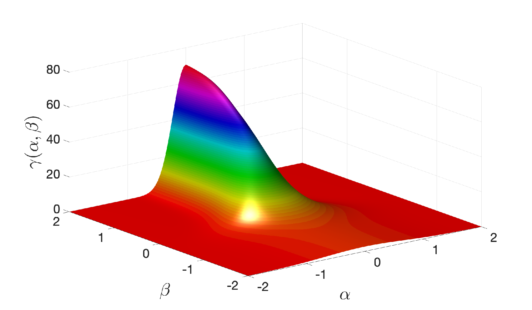
Example 5.3. Here we use the same source term and the initial values as Example 5.2, and consider the following spatially inhomogeneous kernel

γ⁡(y−x,x+y2)=ω⁡(x+y2)ζ3​(x+y2)​H​(y−xζ⁡(x+y2)),\displaystyle\gamma(y-x,\frac{x+y}{2})=\frac{\omega(\frac{x+y}{2})}{\zeta^{3}(\frac{x+y}{2})}H\Big(\frac{y-x}{\zeta(\frac{x+y}{2})}\Big), (4.8)

where

ω⁡(β)=1+e−3​β2,ζ⁡(β)=δ⁡(2+tanh⁡(−1.5​β)),H⁡(s)=4​103π​e−10​s2.\displaystyle\omega(\beta)=1+e^{-3\beta^{2}},\ \zeta(\beta)=\delta(2+\tanh(-1.5\beta)),\ H(s)=4\sqrt{\frac{10^{3}}{\pi}}e^{-10s^{2}}. (4.9)

In the simulations, we take l=2,dp=2l=2,d_{p}=2, the PML coefficient z=10z=10 and μ=|z|,ν=1\mu=|z|,\nu=1.

Refer to caption
Refer to caption
Figure 4.5: (Example 5.3) Left: the functions ω⁡(β)\omega(\beta) and ζ⁡(β)\zeta(\beta). Right: the kernel γ⁡(α,β)\gamma(\alpha,\beta) for δ=1\delta=1.

The limiting local wave equation with PML modifications is given by

∂2u∂t2+z​σ​(x)​∂u∂t−∂v∂x\displaystyle\frac{\partial^{2}u}{\partial t^{2}}+z\sigma(x)\frac{\partial u}{\partial t}-\frac{\partial v}{\partial x} =0,\displaystyle=0, (4.10)
∂v∂t−μ⁡(x)​∂2u∂t​∂x+z​σ​(x)​v\displaystyle\frac{\partial v}{\partial t}-\mu(x)\frac{\partial^{2}u}{\partial t\partial x}+z\sigma(x)v =0.\displaystyle=0. (4.11)

Figure 4.6 shows the evolution of numerical and reference solutions by taking T=4T=4, h=2−8h=2^{-8}, τ=1/12000\tau=1/12000 and m=400m=400 for different δ=0.3,0.2,0.1\delta=0.3,0.2,0.1. Figure 4.7 shows numerical and reference solutions at t=4t=4, which again indicates the numerical solutions decay exponentially in PML layers.

Refer to caption
(a) numerical solution δ=0.3\delta=0.3
Refer to caption
(b) numerical solution δ=0.2\delta=0.2
Refer to caption
(c) numerical solution δ=0.1\delta=0.1
Refer to caption
(d) reference solution δ=0.3\delta=0.3
Refer to caption
(e) reference solution δ=0.2\delta=0.2
Refer to caption
(f) reference solution δ=0.1\delta=0.1
Figure 4.6: (Example 5.3) Numerical solutions for δ=0.3,0.2,0.1\delta=0.3,0.2,0.1 and reference solutions up to T=4T=4. The numerical solutions are obtained by taking h=2−8h=2^{-8} and m=400m=400.
Refer to caption
(a) δ=0.3\delta=0.3
Refer to caption
(b) δ=0.2\delta=0.2
Refer to caption
(c) δ=0.1\delta=0.1
Figure 4.7: (Example 5.3) The comparison of the numerical solution and reference solution at time t=4t=4. The PML layers for numerical solutions are shaded in light grey.

Table 4.5 lists the errors ehe_{h} at t=4t=4 and the spatial convergence order for numerical solutions, which verify the second-order accuracy of the spatial discretization by refining hh. Table 4.6 lists the errors eδe_{\delta} and δ\delta-convergence orders between the numerical solutions and exact solutions of local problem (4.10)–(4.10) by vanishing δ\delta and hh simultaneously at t=2t=2. The behavior of the errors is similar to that shown in the examples above for sufficiently small δ\delta.

hh δ=0.3\delta=0.3 order δ=0.2\delta=0.2 order δ=0.1\delta=0.1 order
2−52^{-5} 3.74e-02 – 4.7483e-02 – 4.35e-02 –
2−62^{-6} 9.96e-03 1.91 1.3050e-02 1.86 1.19e-02 1.87
2−72^{-7} 2.52e-03 1.98 3.3125e-03 1.98 2.99e-03 2.00
2−82^{-8} 6.36e-04 1.98 8.25e-04 2.01 7.21e-04 2.05
Table 4.5: (Example 5.3) errors ehe_{h} and convergence orders at t=4t=4.
hh δ=h\delta=h order δ=2​h\delta=2h order δ=3​h\delta=3h order
2−52^{-5} 5.3521e-02 – 1.1867e-01 – 1.4328e-01 –
2−62^{-6} 1.3937e-02 1.94 4.2328e-02 1.49 8.1629e-02 0.81
2−72^{-7} 3.4432e-03 2.02 1.0714e-02 1.98 2.2952e-02 1.83
2−82^{-8} 8.3835e-04 2.03 2.6479e-03 2.01 5.6996e-03 2.01
Table 4.6: (Example 5.3) The errors eδe_{\delta} and δ\delta-convergence orders between numerical solutions and exact solutions of local PML problem (4.10)–(4.11) by vanishing δ\delta and hh simultaneously at t=2t=2.

5 Conclusion

The nonlocal PML and its numerical discretization of a nonlocal wave equation in unbounded spatial domains are studied in this paper. We first propose the nonlocal PML equation with a time-dependent nonlocal operator which has a complex-valued kernel and is defined by a convolution. This feature differs from the results in [33, 34]. After discretizing the contour integrals arising from the inverse Laplace transform, applying the AC scheme and introducing auxiliary functions, we get a truncated semidiscrete nonlocal PML problem which only involves a finite number of degrees of freedom. A Verlet-type ODE solver is used for the time integration. Numerical experiments demonstrate the effectiveness and accuracy of our proposed PML.

Appendix A.

We first consider Ω𝒦\Omega_{\mathcal{K}} for the kernel (4.4). First, we give the analytic continuation of the reference kernel γ0​(s)=12​c03​e−|s|c0\gamma_{0}(s)=\frac{1}{2c_{0}^{3}}e^{-\frac{|s|}{c_{0}}} by

γ0​(x~−y~)=12​c03​e−ρ⁡(x~,y~)c0,\gamma_{0}(\tilde{x}-\tilde{y})=\frac{1}{2c_{0}^{3}}e^{-\frac{\rho(\tilde{x},\tilde{y})}{c_{0}}},

where ρ⁡(x~,y~)=(x~−y~)2\rho(\tilde{x},\tilde{y})=\sqrt{(\tilde{x}-\tilde{y})^{2}} is its analytic branch ℜ⁡ρ⁡(x~,y~)≥0\Re\rho(\tilde{x},\tilde{y})\geq 0. Let z=z1+i​z2z=z_{1}+\mathrm{i}z_{2} and s=s1+i​s2s=s_{1}+\mathrm{i}s_{2} where z1,z2,s1,s2∈ℝz_{1},z_{2},s_{1},s_{2}\in\mathbb{R}. We have

x~−y~\displaystyle\tilde{x}-\tilde{y} =(x−y)+zs​(∫0xσ⁡(t)​𝑑t−∫0yσ⁡(t)​𝑑t)\displaystyle=(x-y)+\frac{z}{s}\Big(\int_{0}^{x}\sigma(t)\mathrm{d}t-\int_{0}^{y}\sigma(t)\mathrm{d}t\Big)
=(x−y)​[(1+z1​s1+z2​s2|s|2⋅∫0xσ⁡(t)​𝑑t−∫0yσ⁡(t)​𝑑tx−y)​x+i​−z1​s2+z2​s1|s|2⋅∫0xσ⁡(t)​𝑑t−∫0yσ⁡(t)​𝑑tx−y].\displaystyle=(x-y)\Big[\Big(1+\frac{z_{1}s_{1}+z_{2}s_{2}}{|s|^{2}}\cdot\frac{\int_{0}^{x}\sigma(t)\mathrm{d}t-\int_{0}^{y}\sigma(t)\mathrm{d}t}{x-y}\Big)x+\mathrm{i}\frac{-z_{1}s_{2}+z_{2}s_{1}}{|s|^{2}}\cdot\frac{\int_{0}^{x}\sigma(t)\mathrm{d}t-\int_{0}^{y}\sigma(t)\mathrm{d}t}{x-y}\Big].

Set

g=∫0xσ⁡(t)​𝑑t−∫0yσ⁡(t)​𝑑tx−y.g=\frac{\int_{0}^{x}\sigma(t)\mathrm{d}t-\int_{0}^{y}\sigma(t)\mathrm{d}t}{x-y}. (5.1)

It is clear that 0≤g≤10\leq g\leq 1 since σ≤1\sigma\leq 1. Therefore, the real part of x~−y~\tilde{x}-\tilde{y} is

(x−y)​(1+(z1​s1+z2​s2)​g|s|2)\displaystyle(x-y)\Big(1+\frac{(z_{1}s_{1}+z_{2}s_{2})g}{|s|^{2}}\Big) =(x−y)​(|s|2+(z1​s1+z2​s2)​g|s|2)\displaystyle=(x-y)\Big(\frac{|s|^{2}+(z_{1}s_{1}+z_{2}s_{2})g}{|s|^{2}}\Big)
=x−y|s|2​[(s1+z1​g2)2+(s2+z2​g2)2−14​|z|2​g2],\displaystyle=\frac{x-y}{|s|^{2}}\Big[\Big(s_{1}+\frac{z_{1}g}{2}\Big)^{2}+\Big(s_{2}+\frac{z_{2}g}{2}\Big)^{2}-\frac{1}{4}|z|^{2}g^{2}\Big],

which implies that ρ⁡(x~,y~)=(x~−y~)2\rho(\tilde{x},\tilde{y})=\sqrt{(\tilde{x}-\tilde{y})^{2}} as a function of ss is analytic in the ss-domain

Ω𝒦:(s1+z12)2+(s2+z22)2>14​|z|2,∀x,y.\displaystyle\Omega_{\mathcal{K}}:\ \Big(s_{1}+\frac{z_{1}}{2}\Big)^{2}+\Big(s_{2}+\frac{z_{2}}{2}\Big)^{2}>\frac{1}{4}|z|^{2},\quad\forall x,y.

We then consider Talbot’s contour parameters μ\mu and ν\nu for the Gaussian kernel (4.7). The analytic continuation of the kernel γ⁡(y−x,x+y2)=4δ3​103π​e−10​(x−y)2δ2\gamma(y-x,\frac{x+y}{2})=\frac{4}{\delta^{3}}\sqrt{\frac{10^{3}}{\pi}}e^{-10\frac{(x-y)^{2}}{\delta^{2}}} is given by

γ⁡(y~−x~,x~+y~2)=4δ3​103π​e−10​(x~−y~)2δ2.\displaystyle\gamma(\tilde{y}-\tilde{x},\frac{\tilde{x}+\tilde{y}}{2})=\frac{4}{\delta^{3}}\sqrt{\frac{10^{3}}{\pi}}e^{-10\frac{(\tilde{x}-\tilde{y})^{2}}{\delta^{2}}}. (5.2)

Note the Ω𝒦\Omega_{\mathcal{K}} is the whole complex plane for any given z∈ℂz\in\mathbb{C} and x,y∈ℝx,y\in\mathbb{R}. However, to ensure the stability, we have to choose the Talbot’s contour parameters μ\mu and ν\nu such that ℜ⁡[(x~−y~)2]≥0\Re[(\tilde{x}-\tilde{y})^{2}]\geq 0. Denote by ζ=ζ1+i​ζ2=zξj\zeta=\zeta_{1}+\mathrm{i}\zeta_{2}=\frac{z}{\xi_{j}}. We have

ℜ⁡[(x~−y~)2]=\displaystyle\Re\Big[(\tilde{x}-\tilde{y})^{2}\Big]= ℜ⁡[((x+ζ1​∫0xσ⁡(t)​𝑑t+i​ζ2​∫0xσ⁡(t)​𝑑t)−(y+ζ1​∫0yσ⁡(t)​𝑑t+i​ζ2​∫0yσ⁡(t)​𝑑t))2]\displaystyle\Re\Big[\Big((x+\zeta_{1}\int_{0}^{x}\sigma(t)\mathrm{d}t+\mathrm{i}\zeta_{2}\int_{0}^{x}\sigma(t)\mathrm{d}t)-(y+\zeta_{1}\int_{0}^{y}\sigma(t)\mathrm{d}t+\mathrm{i}\zeta_{2}\int_{0}^{y}\sigma(t)\mathrm{d}t)\Big)^{2}\Big]
=\displaystyle= ((x+ζ1​∫0xσ⁡(t)​𝑑t)−(y+ζ1​∫0yσ⁡(t)​𝑑t))2−(ζ2​∫0xσ⁡(t)​𝑑t−ζ2​∫0yσ⁡(t)​𝑑t)2\displaystyle\Big((x+\zeta_{1}\int_{0}^{x}\sigma(t)\mathrm{d}t)-(y+\zeta_{1}\int_{0}^{y}\sigma(t)\mathrm{d}t)\Big)^{2}-\Big(\zeta_{2}\int_{0}^{x}\sigma(t)\mathrm{d}t-\zeta_{2}\int_{0}^{y}\sigma(t)\mathrm{d}t\Big)^{2}
=\displaystyle= (x−y)2​[(1+ζ1​g)2−ζ22​g2]\displaystyle(x-y)^{2}\big[(1+\zeta_{1}g)^{2}-\zeta_{2}^{2}g^{2}\big]
=\displaystyle= (x−y)2​[(1+(ζ1−ζ2)​g)​(1+(ζ1+ζ2)​g)],\displaystyle(x-y)^{2}\big[\big(1+(\zeta_{1}-\zeta_{2})g\big)\big(1+(\zeta_{1}+\zeta_{2})g\big)\big],

where gg is defined in (5.1) with 0≤g≤10\leq g\leq 1 as 0≤σ≤10\leq\sigma\leq 1.

To ensure ℜ⁡[(x~−y~)2]≥0\Re[(\tilde{x}-\tilde{y})^{2}]\geq 0, we have (1+(ζ1−ζ2)​g)​(1+(ζ1+ζ2)​g)≥0\big(1+(\zeta_{1}-\zeta_{2})g\big)\big(1+(\zeta_{1}+\zeta_{2})g\big)\geq 0 for any g∈[0,1]g\in[0,1], which implies that ζ1−ζ2≥−1\zeta_{1}-\zeta_{2}\geq-1 and ζ1+ζ2≥−1\zeta_{1}+\zeta_{2}\geq-1. Therefore, we may simply choose Talbot’s contour parameters μ\mu and ν\nu such that

2|z|≤|ξj|,∀j=1,2,⋯,m.\displaystyle\sqrt{2}|z|\leq|\xi_{j}|,\quad\forall\ j=1,2,\cdots,m. (5.3)

References

  • [1] X. Antoine and E. Lorin, Towards perfectly matched layers for time-dependent space fractional PDEs, J. Comput. Phys., 391 (2019), pp. 59–90.
  • [2] U. Basu, Perfectly matched layers for acoustic and elastic waves, Dam Safety Research Program, US Department of the Interior, (2008).
  • [3] E. Becache, A. B.-B. Dhia, and G. Legendre, Perfectly matched layers for the convected Helmholtz equation, SIAM J. Numer. Anal., 42 (2004), pp. 409–433.
  • [4] J.-P. Bérenger, A perfectly matched layer for the absorption of electromagnetic waves, J. Comput. Phys., 114 (1994), pp. 185–200.
  • [5]  , Three-dimensional perfectly matched layer for the absorption of electromagnetic waves, J. Comput. Phys., 127 (1996), pp. 363–379.
  • [6] A. Bermudez, L. Hervella-Nieto, A. Prieto, and R. Rodriguez, An exact bounded perfectly matched layer for time-harmonic scattering problems, SIAM J. Sci. Comput., 30 (2007), pp. 312–338.
  • [7] F. Bobaru, Influence of van der waals forces on increasing the strength and toughness in dynamic fracture of nanofibre networks: a peridynamic approach*, Model Simul. Mat. Sci. Eng., 15 (2007), pp. 397–417.
  • [8] F. Bobaru and M. Duangpanya, The peridynamic formulation for transient heat conduction, Int. J. Heat Mass Transf., 53 (2010), pp. 4047–4059.
  • [9] F. Bobaru, M. Yang, L. F. Alves, S. A. Silling, E. Askari, and J. Xu, Convergence, adaptive refinement, and scaling in 1D peridynamics, Int. J. Numer. Methods Eng., 77 (2009), pp. 852–877.
  • [10] W. Chen and W. Weedom, A 3D perfectly Matched medium from modified Maxwell’s equations with stretched coordinates, Microwave Opt. Tech. Lett., 7 (1994), pp. 599–604.
  • [11] Z. Chen and X. Liu, An adaptive perfectly matched layer technique for time-harmonic scattering problems, SIAM J. Numer. Anal., 41 (2003), pp. 799–826.
  • [12] F. Collino and P. Monk, The perfectly matched layer in curvilinear coordinates, SIAM J. Sci. Comput., 19 (1998), pp. 2061–2090.
  • [13] Q. Du, Local limits and asymptotically compatible discretizations, in Handbook of Peridynamic Modeling, Adv. Appl. Math., CRC Press, Boca Raton, FL, 2017.
  • [14] Q. Du, M. D. Gunzburger, R. B. Lehoucq, and K. Zhou, Analysis and approximation of nonlocal diffusion problems with volume constraints, Siam Rev., 54 (2012), pp. 667–696.
  • [15] Q. Du, H. Han, J. Zhang, and C. Zheng, Numerical solution of a two-dimensional nonlocal wave equation on unbounded domains, SIAM J. Sci. Comput., 40 (2018), pp. 1430–1445.
  • [16] Q. Du, Y. Tao, X. Tian, and J. Yang, Asymptotically compatible discretization of multidimensional nonlocal diffusion models and approximation of nonlocal Green’s functions, IMA J. NUMER. ANAL., 39 (2019), pp. 607–625.
  • [17] Q. Du, J. Zhang, and C. Zheng, Nonlocal wave propagation in unbounded multiscale media, Comm. Comp. Phys., 24 (2018), pp. 1049–1072.
  • [18] Y. Du and J. Zhang, Numerical solution of a one-dimensional nonlocal Helmholtz equation by perfectly matched layers, arXiv preprint arXiv:2007.11193, (2020).
  • [19]  , Perfectly matched layers for nonlocal Helmholtz equations II: multi-dimensional cases, arXiv preprint arXiv:2012.01753, (2020).
  • [20] J. T. Foster, S. A. Silling, and W. W. Chen, Viscoplasticity using peridynamics, Int. J. Numer. Methods Eng., 81 (2010), pp. 1242–1258.
  • [21] W. Gerstle, N. Sau, and E. Aguilera, Micropolar peridynamic constitutive model for concrete, 19th International Conference on Structural Mechanics in Reactor Technology, (2007), pp. 1–8.
  • [22] S. Ji, G. Pang, X. Antoine, and J. Zhang, Artificial boundary conditions for the semi-discretized one-dimensional nonlocal Schrödinger equation, J. Comput. Phys., accepted, (2020).
  • [23] S. A. Silling, Reformulation of elasticity theory for discontinuities and long-range forces, J. Mech. Phys. Solids, 48 (2000), pp. 175–209.
  • [24] H. Tian, L. Ju, and Q. Du, A conservative nonlocal convection–diffusion model and asymptotically compatible finite difference discretization, Comput. Methods Appl. Mech. Eng., 320 (2017), pp. 46–67.
  • [25] X. Tian and Q. Du, Analysis and comparison of different approximations to nonlocal diffusion and linear peridynamic equations, SIAM J. Numer. Anal., 51 (2013), pp. 3458–3482.
  • [26]  , Asymptotically compatible schemes and applications to robust discretization of nonlocal models, SIAM J. Numer. Anal., 52 (2014), pp. 1641–1665.
  • [27] X. Tian and Q. Du, Asymptotically compatible schemes and applications to robust discretization of nonlocal models, SIAM J. Numer. Anal., 52 (2014), pp. 1641–1665.
  • [28] E. Turkel and A. Yefet, Absorbing pml boundary Layers for wave-like equations, Appl. Numer. Math., 27 (1998), pp. 533–557.
  • [29] X. Wang and S. Tang, Matching boundary conditions for lattice dynamics, Int. J. Numer. Methods Eng., 93 (2013), pp. 1255–1285.
  • [30] O. Weckner and R. Abeyaratne, The effect of long-range forces on the dynamics of a bar, J. Mech. Phys. Solids, 53 (2005), pp. 705–728.
  • [31] O. Weckner, G. Brunk, M. A. Epton, S. A. Silling, and E. Askari, Green’s functions in non-local three-dimensional linear elasticity, P. Roy. Soc. A-Math. Phy., 465 (2009), pp. 3463–3487.
  • [32] J. A. C. Weideman, Optimizing Talbot’s contours for the inversion of the Laplace transform, SIAM J. Numer. Anal., 44 (2006), pp. 2342–2362.
  • [33] R. A. Wildman and G. A. Gazonas, A perfectly matched layer for peridynamics in one dimension, Technical report ARL-TR-5626, U.S. Army Research Laboratory, Aberdeen, MD, (2011).
  • [34]  , A perfectly matched layer for peridynamics in two dimensions, J. Mech. Mater. Struct., 7 (2012), pp. 765–781.
  • [35] W. Zhang, J. Yang, J. Zhang, and Q. Du, Absorbing boundary conditions for nonlocal heat equations on unbounded domain, Commun. Comput. Phys., 21 (2017), pp. 16–39.
  • [36] C. Zheng, Q. Du, X. Ma, and J. Zhang, Stability and error analysis for a second-order fast approximation of the local and nonlocal diffusion equations on the real line, SIAM J. Numer. Anal., 58 (2020), pp. 1893–1917.
  • [37] C. Zheng, J. Hu, Q. Du, and J. Zhang, Numerical solution of the nonlocal diffusion equation on the real line, SIAM J. Sci. Comput., 39 (2017), pp. 1951–1968.
  • [38] K. Zhou and Q. Du, Mathematical and numerical analysis of linear peridynamic models with nonlocal boundary conditions, SIAM J. Numer. Anal., 48 (2010), pp. 1759–1780.